Deep Theory of Functional Connections: A New Method for ...

machine learning &

knowledge extraction

Article

Deep Theory of Functional Connections: A NewMethod for Estimating the Solutions of PartialDifferential Equations

Carl Leake * and Daniele Mortari

Aerospace Engineering, Texas A&M University, College Station, TX 77843, USA; [email protected]* Correspondence: [email protected]

Received: 11 February 2020; Accepted: 9 March 2020; Published: 12 March 2020

Abstract: This article presents a new methodology called Deep Theory of Functional Connections(TFC) that estimates the solutions of partial differential equations (PDEs) by combining neuralnetworks with the TFC. The TFC is used to transform PDEs into unconstrained optimization problemsby analytically embedding the PDE’s constraints into a “constrained expression” containing a freefunction. In this research , the free function is chosen to be a neural network, which is used to solvethe now unconstrained optimization problem. This optimization problem consists of minimizinga loss function that is chosen to be the square of the residuals of the PDE. The neural networkis trained in an unsupervised manner to minimize this loss function. This methodology has twomajor differences when compared with popular methods used to estimate the solutions of PDEs.First, this methodology does not need to discretize the domain into a grid, rather, this methodologycan randomly sample points from the domain during the training phase. Second, after training,this methodology produces an accurate analytical approximation of the solution throughout the entiretraining domain. Because the methodology produces an analytical solution, it is straightforward toobtain the solution at any point within the domain and to perform further manipulation if needed,such as differentiation. In contrast, other popular methods require extra numerical techniques if theestimated solution is desired at points that do not lie on the discretized grid, or if further manipulationto the estimated solution must be performed.

Keywords: deep learning; neural network; theory of functional connections; partialdifferential equation

1. Introduction

Partial differential equations (PDEs) are a powerful mathematical tool that is used to modelphysical phenomena, and their solutions are used to simulate, design, and verify the design of a varietyof systems. PDEs are used in multiple fields including environmental science, engineering, finance,medical science, and physics, to name a few. Many methods exist to approximate the solutions ofPDEs. The most famous of these methods is the finite element method (FEM) [1–3]. FEM has beenincredibly successful in approximating the solution to PDEs in a variety of fields including structures,fluids, and acoustics. However, FEM does have some drawbacks.

FEM discretizes the domain into elements. This works well for low-dimensional cases, but thenumber of elements grows exponentially with the number of dimensions. Therefore, the discretizationbecomes prohibitive as the number of dimensions increases. Another issue is that FEM solvesthe PDE at discrete nodes, but if the solution is needed at locations other than these nodes,an interpolation scheme must be used. Moreover, extra numerical techniques are needed to performfurther manipulation of the FEM solution.

Mach. Learn. Knowl. Extr. 2020, 2, 37–55; doi:10.3390/make2010004 www.mdpi.com/journal/make

http://www.mdpi.com/journal/make

http://www.mdpi.com

https://orcid.org/0000-0002-3750-5067

https://orcid.org/0000-0003-0787-4547

http://dx.doi.org/10.3390/make2010004

http://www.mdpi.com/journal/make

Mach. Learn. Knowl. Extr. 2020, 2 38

Reference [4] explored the use of neural networks to solve PDEs, and showed that the use of neuralnetworks avoids these problems. Rather than discretizing the entire domain into a number of elementsthat grows exponentially with the dimension, neural networks can sample points randomly from thedomain. Moreover, once the neural network is trained, it represents an analytical approximation of thePDE. Consequently, no interpolation scheme is needed when estimating the solution at points thatdid not appear during training, and further analytical manipulation of the solution can be done withease. Furthermore, Ref. [4] compared the neural network method with FEM on a set of test points thatdid not appear during training (i.e., points that were not the nodes in the FEM solution), and showedthat the solution obtained by the neural network generalized well to points outside of the trainingdata. In fact, the maximum error on the test set of data was never more than the maximum error onthe training set of data. In contrast, the FEM had more error on the test set than on the training set.In one case, the test set had approximately three orders of magnitude more error than the training set.In short, Ref. [4] presents strong evidence that neural networks are useful for solving PDEs.

However, what was presented in Ref. [4] can still be improved. In Ref. [4] the boundary constraintsare managed by adding extra terms to the loss function. An alternative method is to encapsulate theboundary conditions, by posing the solution in such a way that the boundary conditions must besatisfied, regardless of the values of the training parameters in the neural network. References [5,6]manage boundary constraints in this way when solving PDEs with neural networks by using a methodsimilar to the Coons’ patch [7] to satisfy the boundary constraints exactly.

Exact boundary constraint satisfaction is of interest for a variety of problems, particularly whenconfidence in the constraint information is high. This is especially important for physics informedproblems. Moreover, embedding the boundary conditions in this way means that the neuralnetwork needs to sample points from the interior of the domain only, not the domain and theboundary. While the methods presented in [5,6] work well for low-dimensional PDEs withsimple boundary constraints, they lack a mechanized framework for generating expressions thatembed higher-dimensional or more complex constraints while maintaining a neural network withfree-to-choose parameters. For example, the fourth problem in the results section cannot be solvedusing the solution forms shown in Ref. [5,6]. Luckily, a framework that can embed higher-dimensionalor more complex constraints has already been invented: The Theory of Functional Connections(TFC) [8,9]. In Ref. [10], TFC was used to embed constraints into support vector machines, but leftembedding constraints into neural networks to future work. This research shows how to embedconstraints into neural networks with the TFC, and leverages this technique to numerically estimatethe solutions of PDEs. Although the focus of this article is a new technique for numerically estimatingthe solutions of PDEs, the article’s contribution to the machine learning community is farther reaching,as the ability to embed constraints into neural networks has the potential to improve performancewhen solving any problem that has constraints, not just differential equations, with neural networks.

TFC is a framework that is able to satisfy many types of boundary conditions while maintaininga function that can be freely chosen. This free function can be chosen, for example, to minimizethe residual of a differential equation. TFC has already been used to solve ordinary differentialequations with initial value constraints, boundary value constraints, relative constraints, integralconstraints, and linear combinations of constraints [8,11–13]. Recently, the framework was extended ton-dimensions [9] for constraints on the value and arbitrary order derivative of (n− 1)-dimensionalmanifolds. This means the TFC framework can now generate constrained expressions that satisfy theboundary constraints of multidimensional PDEs [14].

2. Theory of Functional Connections

The Theory of Functional Connections (TFC) is a mathematical framework designed to turnconstrained problems into unconstrained problems. This is accomplished through the use ofconstrained expressions, which are functionals that represent the family of all possible functionsthat satisfy the problem’s constraints. This technique is especially useful when solving PDEs, as it


reduces the space of solutions to just those that satisfy the problem’s constraints. TFC has two majorsteps: (1) Embed the boundary conditions of the problem into the constrained expression; (2) solvethe now unconstrained optimization problem. The paragraphs that follow will explain these steps inmore detail.

The TFC framework is easiest to understand when explained via an example, like a simpleharmonic oscillator. Equation (1) gives an example of a simple harmonic oscillator problem.

md2ydx2

1+ k y = 0 subject to:

{y(0) = y0

yx1(0) = yx1 ,(1)

where the subscript in yx1 denotes a derivative of y with respect to x1.Based on the univariate TFC framework presented in Ref. [8], the constrained expression is

represented by the functional,

f (x1, g(x1)) = g(x1) +2

∑j=1

ηj sj(x1),

where the sj(x1) are a set of mutually linearly independent functions, called support functions, and ηjare coefficient functions that are computed by imposing the constraints. For this example, let’s choosethe support functions to be the first two monomials, s1(x1) = 1 and s2(x1) = x1. Hence, the constrainedexpression becomes,

f (x1, g(x1)) = g(x1) + η1 + x1 η2. (2)

The coefficient functions, η1(x1) and η2(x1), are solved by substituting the constraints into theconstrained expression and solving the resultant set of equations. For the simple harmonic oscillatorthis yields the set of equations given by Equations (3) and (4).

y(0) = g(0) + η1 (3)

yx1(0) = gx1(0) + η2. (4)

Solving Equation (3) results in η1 = y(0)− g(0), and solving Equation (4) yields η2 = yx1(0)−gx1(0). Substituting η1 and η2 into Equation (3) we obtain,

f (x1, g(x1)) = g(x1) + y(0)− g(0) + x1

[yx1(0)− gx1(0)

]which is an expression satisfying the constraints, no matter what the free function, g(x1), is. In otherwords, this equation is able to reduce the solution space to just the space of functions satisfyingthe constraints, because for any function g(x1), the boundary conditions will always be satisfiedexactly. Therefore, using constrained expressions transforms differential equations into unconstrainedoptimization problems.

This unconstrained optimization problem could be cast in the following way. Let the function tobe minimized, L, be equal to the square of the residual of the differential equation,

L(x1) =

[m

d2 f (x1, g(x1))

dx21

+ k f (x1)

]2

.

This function is to be minimized by varying the function g(x1). One way to do this is to chooseg(x1) as a linear combination of a set of basis functions, and calculate the coefficients of the linearcombination via least-squares or some other optimization technique. Examples of this methodologyusing Chebyshev orthogonal polynomials to obtain least-squares solutions of linear and nonlinearordinary differential equations (ODEs) can be found in Refs. [11,12], respectively.


2.1. n-Dimensional Constrained Expressions

The previous example derived the constrained expression by creating and solving a seriesof simultaneous algebraic equations. This technique works well for constrained expressions inone dimension; however, it can become needlessly complicated when deriving these expressionin n dimensions for constraints on the value and arbitrary order derivative of n − 1 dimensionalmanifolds [9]. Fortunately, a different, more mechanized formalism exists that is useful for this case.The constrained expression presented earlier consists of two parts; the first part is a function thatsatisfies the boundary constraints, and the second part projects the free-function, g(x1), onto thehyper-surface of functions that are equal to zero at the boundaries. Rearranging Equation (2) highlightsthese two parts,

f (x1, g(x1)) = y(0) + x1yx1(0)︸︷︷︸A(x1)

+ g(x1)− g(0)− x1gx1(0)︸︷︷︸B(x1,g(x1))

,

where A(x1) satisfies the boundary constraints and B(x1, g(x1)) is a functional projecting thefree-function onto the hyper-surface of functions that are equal to zero at the boundaries.

The multivariate extension of this form for problems with boundary and derivative constraints inn-dimensions can be written compactly using Equation (5).

f (x, g(x)) = Mi1,i2,··· ,in(c(x))vi1(x1)vi2(x2) · · · vin(xn)︸︷︷︸A(x)

+ (5)

+ g(x)−Mi1,i2,··· ,in(g(x))vi1(x1)vi2(x2) · · · vin(xn)︸︷︷︸B(x,g(x))

where x = {x1, x2, · · · , xn}T is a vector of the n independent variables,M is an n-th order tensorcontaining the boundary conditions c(x), the vi1 , · · · , vin are vectors whose elements are functions ofthe independent variables, g(x) is the free-function that can be chosen to be any function that is definedat the constraints, and f (x, g(x)) is the constrained expression. The first term, A(x), analyticallysatisfies the boundary conditions, and the term, B(x, g(x)), projects the free-function, g(x), onto thespace of functions that vanish at the constraints. A mathematical proof that this form of the constrainedexpression satisfies the boundary constraints is given in Ref. [9]. The remainder of this section discusseshow to construct the n-th order tensorM and the v vectors shown in Equation (5).

Before discussing how to build theM tensor and v vectors, let’s introduce some mathematical

notation. Let k ∈ [1, n] be an index used to denote the k-th dimension. Let kcdp :=

∂dc(x)∂xd

k

∣∣∣∣xk=p

be

the constraint specified by taking the d-th derivative of the constraint function, c(x), evaluated at thexk = p hyperplane. Further, let kcdk

pkbe the vector of `k constraints defined at the xk = pk hyperplanes

with derivative orders of dk, where pk and dk ∈ R`k . In addition, let’s define a boundary conditionoperator kbd

p that takes the d-th derivative with respect to xk of a function, and then evaluates thatfunction at the xk = p hyperplane. Mathematically,

kbdp[ f (x)] =

∂d f (x)∂xd

k

∣∣∣∣xk=p

.

This mathematical notation will be used to introduce a step-by-step method for building theM tensor. This step-by-step process will be be illustrated via a 3-dimensional example that hasDirichlet boundary conditions in x1 and initial conditions in x2 and x3 on the domain x1, x2, x3 ∈[0, 1]× [0, 1]× [0, 1]. TheM tensor is constructed using the following three rules.

1. The elementM111 = 0.


2. The first order sub-tensor of M specified by keeping one dimension’s index free and settingall other dimension’s indices to 1 consists of the value 0 and the boundary conditions for thatdimension. Mathematically,

M1,...,1,ik ,1,...,1 ={

0,k cdkpk

}.

Using the example boundary conditions,

Mi111 =[0, c(0, x2, x3), c(1, x2, x3)

]T

M1i21 =[0, c(x1, 0, x3), cx2(x1, 0, x3)

]T (6)

M11i3 =[0, c(x1, x2, 0), cx3(x1, x2, 0)

]T.

3. The remaining elements of theM tensor are those with at least two indices different than one.These elements are the geometric intersection of the boundary condition elements of the firstorder tensors given in Equation (6), plus a sign (+ or −) that is determined by the number ofelements being intersected. Mathematically this can be written as,

Mi1i2 ...in = 1bd1

i1−1

p1i1−1

[2b

d2i2−1

p2i2−1

[. . .[

nbdn

in−1pn

in−1[c(x)]

]. . .]]

(−1)m+1,

where m is the number of indices different than one. Using the example boundary conditions wegive three examples:

M133 = −cx2x3(x1, 0, 0)

M221 = −c(0, 0, x3)

M332 = cx2(1, 0, 0)

A simple procedure also exists for constructing the vik vectors. The vik vectors have astandard form:

vik =

{1,

`k

∑i=1

αi1 hi(xk),`k

∑i=1

αi2 hi(xk), . . . ,`k

∑i=1

αi`khi(xk)

}T

,

where hi(xk) are `k linearly independent functions. The simplest set of linearly independent functions,and those most often used in the TFC constrained expressions, are monomials, hi(xk) = xi−1

k . The `k ×`k coefficients, αij, can be computed by matrix inversion,

kbd1p1 [h1]

kbd1p1 [h2] . . . kbd1

p1 [h`k]

kbd2p2 [h1]

kbd2p2 [h2] . . . kbd2

p2 [h`k]

......

. . ....

kbd`kp`k

[h1]kb

d`kp`k

[h2] . . . kbd`kp`k

[h`k]

α11 α12 . . . α1`k

α21 α22 . . . α2`k...

.... . .

...α`k1 α`k2 . . . α`k`k

=

1 0 . . . 00 1 . . . 0...

.... . .

...0 0 . . . 1

.

Using the example boundary conditions, let’s derive the vi1 vector using the linearly independentfunctions h1 = 1 and h2 = x1.[

1 01 1

] [α11 α12

α21 α22

]=

[1 00 1

]→

[α11 α12

α21 α22

]=

[1 0−1 1

]

vi1 ={

1, 1− x1, x1

}T

.


For more examples and a mathematical proof that these procedures for generating theM tensorand the v vectors form a valid constrained expression see Ref. [9].

2.2. Two-Dimensional Example

This subsection will give an in depth example for a two-dimensional TFC case. The exampleis originally from problem 5 of Ref. [5], and is one of the PDE problems analyzed in this article.The problem is shown in Equation (7).

∇2z(x, y) = e−x(x− 2 + y3 + 6y) subject to:z(x, 0) = c(x, 0) = xe−x

z(0, y) = c(0, y) = y3

z(x, 1) = c(x, 1) = e−x(x + 1)

z(1, y) = c(1, y) = (1 + y3)e−1

where (x, y) ∈ [0, 1]× [0, 1]

(7)

Following the step-by-step procedure given in the previous section we will construct theM tensor:

1. The first element isM11 = 0.2. The first order sub-tensors ofM are:

Mi11 ={

0 c(0, y) c(1, y)}

M1i2 ={

0 c(x, 0) c(x, 1)}

3. The remaining elements of M are the geometric intersection of elements from the first ordersub-tensors.

M22 = −c(0, 0) M23 = −c(1, 0)

M32 = −c(0, 1) M33 = −c(1, 1)

Hence, theM tensor is,

Mi1i2 =

0 c(0, y) c(1, y)c(x, 0) −c(0, 0) −c(1, 0)c(x, 1) −c(0, 1) −c(1, 1)

=

0 y3 (1 + y3)e−1

xe−x 0 −e−1

e−x(x + 1) −1 −2e−1

Following the step-by-step procedure given in the previous section we will construct the v vectors.

For vi1 , let’s choose the linearly independent functions h1 = 1 and h2 = x.[1 01 1

] [α11 α12

α21 α22

]=

[1 00 1

]→

[α11 α12

α21 α22

]=

[1 0−1 1

]

vi1 ={

1, 1− x, x}T

.

For vi2 let’s choose the linearly indpendent functions h1 = 1 and h2 = y.[1 01 1

] [α11 α12

α21 α22

]=

[1 00 1

]→

[α11 α12

α21 α22

]=

[1 0−1 1

]

vi2 ={

1, 1− y, y}T

.


Now, we use the constrained expression form given in Equation (5) to finish building theconstrained expression.

f (x, y, g(x, y)) = g(x, y) +xy(y2 − 1)

e+ e−x(x + y)+ (8)

+ (1− x)(

g(0, 0) + y(

g(0, 1) + y2 − g(0, 0)− 1))

+ (x− 1)g(0, y)+

+ x(

yg(1, 1) + (1− y)g(1, 0))− xg(1, y) + (y− 1)g(x, 0)− yg(x, 1)

Notice, that Equation (8) will always satisfy the boundary conditions of the problem regardlessof the value of g(x, y). Thus, the problem has been transformed into an unconstrained optimizationproblem where the cost function, L, is the square of the residual of the PDE,

L(x, y, g(x, y)) =(∇2 f (x, y, g(x, y))− e−x(x− 2 + y3 + 6y)

)2.

For ODEs, the minimization of the cost function was accomplished by choosing g to be a linearcombination of orthogonal polynomials with unknown coefficients, and performing least-squares orsome other optimization technique to find the unknown coefficients. For two dimensions, one couldmake g(x, y) the product of two linear combinations of these orthogonal polynomials, calculate allof the cross-terms, and then solve for the coefficients that multiply all terms and cross-terms usingleast-squares or non-linear least-squares. However, this will become computationally prohibitive asthe dimension increases. Even at two dimensions, the number of basis functions needed, and thus thesize of the matrix to invert in the least-squares, becomes large. An alternative solution, and the oneexplored in this article, is to make the free function, g(x, y), a neural network.

3. PDE Solution Methodology

Similar to the last section, the easiest way to describe the methodology is with an example.The example used throughout this section will be the PDE given in Equation (7).

As mentioned previously, Deep TFC approximates solutions to PDEs by finding the constrainedexpression for the PDE and choosing a neural network as the free function. For all of the problemsanalyzed in this article, a simple, fully connected neural network was used. Each layer of afully connected neural network consists of non-linear activation functions composed with affinetransformations of the form A = W · x + b, where W is a matrix of the neuron weights, b is a vectorof the neuron biases, and x is a vector of inputs from the previous layer (or the inputs to the neuralnetwork if it is the first layer). Then, each layer is composed to form the entire network. For the fullyconnected neural networks used in this paper, the last layer is simply a linear output layer. For example,a neural network with three hidden layers that each use the non-linear activation function φ can bewritten mathematically as,

N (x; θ) = W4 · φ(

W3 · φ(

W2 · φ(W1 · x + b1

)+ b2

)+ b3

)+ b4,

where N is the symbol used for the neural network, x is the vector of inputs, Wk are the weightmatrices, bk are the bias vectors, and θ is a symbol that represents all trainable parameters of theneural network; the weights and biases of each layer constitute the trainable parameters. Note thatthe notation N (x, y, . . . ; θ) is also used in this paper for independent variables x, y, . . . and trainableparameters θ.


Thus, the constrained expression, given originally in Equation (8), now has the form given inEquation (9).

f (x, y; θ) = N (x, y; θ) +xy(y2 − 1)

e+ e−x(x + y)+

+ (1− x)(N (0, 0; θ) + y

(N (0, 1; θ) + y2 −N (0, 0; θ)− 1

))+ (x− 1)N (0, y; θ)+

+ x(

yN (1, 1; θ) + (1− y)N (1, 0; θ))− xN (1, y; θ) + (y− 1)N (x, 0; θ)− yN (x, 1; θ)

(9)

In order to estimate the solution to the PDE, the parameters of the neural network have to beoptimized to minimize the loss function, which is taken to be the square of the residual of the PDE.For this example,

L =N

∑iLi(xi, yi; θ) where Li(xi, yi; θ) =

(∇2 f (xi, yi; θ)− e−xi (xi − 2 + y3

i + 6yi))2

.

The attentive reader will notice that training the neural network will require, for this example,taking two second order partial derivatives of f (x, y; θ) to calculate Li, and then taking gradients of Lwith respect to the neural network parameters, θ, in order to train the neural network.

To take these higher order derivatives, TensorFlow’sTM gradients function was used [15].This function uses automatic differentiation [16] to compute these derivatives. However, one must beconscientious when using the gradients function to ensure they get the desired gradients.

When taking the gradient of a vector, yj, with respect to another vector, xi,TensorFlowTMc̃omputes,

zi =∂

∂xi

( N

∑j=1

yj

)where zi is a vector of the same size as xi. The only example where it is not immediately obvious thatthis gradient function will give the desired gradient is when computing ∇2 fi. The desired output ofthis calculation is the following vector,

zi =

{∂2 f1

∂x21+

∂2 f1

∂y21

, · · · ,∂2 fN

∂x2N

+∂2 fN

∂y2N

}T

,

where zi has the same size as fi and (xi, yi) is the point used to generate fi. TensorFlow’sTM gradientsfunction will compute the following vector,

z̃i =

{∂2(∑N

j=1 f j)

∂x21

+∂2(∑N

j=1 f j)

∂y21

, · · · ,∂2(∑N

j=1 f j)

∂x2N

+∂2(∑N

j=1 f j)

∂y2N

}T

.

However, because fi only depends on the point (xi, yi) and the derivative operator commuteswith the sum operator, TensorFlow’sTM gradients function will compute the desired vector (i.e., z̃i = zi).Moreover, the size of the output vector will be correct, because the input vectors, xi and yi, have thesame size as fi.

Training the Neural Network

Three methods were tested when optimizing the parameters of the neural networks:

1. Adam optimizer [17]: A variant of stochastic gradient descent (SGD) that combines the advantagesof two other popular SGD variants: AdaGrad [18] and RMSProp [19].


2. Broyden-–Fletcher—Goldfarb-–Shanno [20] (BFGS): A quasi-Newton method designed for solvingunconstrained, non-linear optimization problems. This method was chosen based on itsperformance when optimizing neural network parameters to estimate PDE solutions in Ref. [5].

3. Hybrid method: Combines the first two methods by applying them in series.

For all four problems shown in this article, the solution error when using the BFGS optimizerwas lower than with the other two methods. Thus, in the following section, the results shown use theBFGS optimizer.

The BFGS optimizer is a local optimizer, and the weights and biases of the neural networks areinitialized randomly. Therefore, the solution error when numerically estimating PDEs will be differenteach time. However, Deep TFC guarantees that the boundary conditions are satisfied, and the lossfunction is the square of the residual of the PDE. Therefore, the loss function indicates how wellDeep TFC is estimating the solution of the PDE at the training points. Moreover, because Deep TFCproduces an analytical approximation of the solution, the loss function can be calculated at any point.Therefore, after training, one can calculate the loss function at a set of test points to determine whetherthe approximate solution generalizes well or has over fit the training points.

Due to the inherit stochasticity of the method, each Deep TFC solution presented in the resultssection that follows is the solution with the lowest mean absolute error of 10 trials. In other words,for each problem, the Deep TFC methodology was performed 10 times, and the best solution of those10 trials is presented. Moreover, to show the variability in the Deep TFC method, problem 1 contains ahistogram of the maximum solution error on a test set for 100 Monte Carlo trials.

4. Results

This section compares the estimated solution found using Deep TFC with with the analyticalsolution. Four PDE problems are analyzed. The first is the example PDE given in Equation (7), and thesecond is the wave equation. The third and fourth PDEs are simple solutions to the incompressibleNavier–Stokes equations.

4.1. Problem 1

The first problem analyzed was the PDE given by Equation (7), copied below for thereader’s convenience.

∇2z(x, y) = e−x(x− 2 + y3 + 6y) subject to:z(x, 0) = xe−x

z(0, y) = y3

z(x, 1) = e−x(x + 1)

z(1, y) = (1 + y3)e−1

where (x, y) ∈ [0, 1]× [0, 1]

The known analytical solution for this problem is,

z = e−x(x + y3).

The neural network used to estimate the solution to this PDE was a fully connected neuralnetwork with 6 hidden layers, 15 neurons per layer, and 1 linear output layer. The non-linear activationfunction used in the hidden layers was the hyperbolic tangent. Other fully connected neural networkswith various sizes and non-linear activation functions were tested, but this combination of size andactivation function performed the best in terms of solution error. The biases of the neural networkwere all initialized as zero, and the weights were initialized using TensorFlow’sTM implementation ofthe Xavier initialization with uniform random initialization [21]. One hundred training points, (x, y),evenly distributed throughout the domain were used to train the neural network.


Figure 1 shows the difference between the analytical solution and the estimated solution usingDeep TFC on a grid of 10,000 evenly distributed points. This grid represents the test set. Figure 2shows a histogram of the maximum solution error on the test set for 100 Monte Carlo trials.

x

0.00.2

0.40.6

0.81.0

y

0.00.2

0.40.6

0.81.0

|zz t

rue|

1e7

0.0

0.5

1.0

1.5

2.0

2.5

5.00e-08

1.00e-07

1.50e-07

2.00e-07

2.50e-07

Figure 1. Problem 1 solution error.

10 7 10 6 10 5

Max Error0

2

4

6

8

10

12

Num

ber o

f Occ

uran

ces

Figure 2. Problem 1 maximum test set solution error from 100 Monte Carlo trials.

The maximum error on the test set shown in Figure 1 was 2.780× 10−7 and the average error was8.517× 10−8. Figure 2 shows that Deep TFC produces a solution at least as accurate as the solutionin Figure 1 approximately 10% of the time. The remaining 90% of the time the solution error will belarger. Moreover, Figure 2 shows that the Deep TFC method is consistent. The maximum solutionerror in the 100 Monte Carlo tests was 3.891× 10−6, approximately an order of magnitude largerthan the maximum solution error shown in Figure 1. The maximum error from Figure 1 is relatively


low, six orders of magnitude lower than the solution values, which are on the order of 10−1. Table 1compares the maximum error on the test and training sets obtained with Deep TFC with the methodused in Ref. [5] and FEM. Note, the FEM data was obtained from Table 1 of Ref. [5].

Table 1. Comparison of Deep TFC, Ref. [5], and finite element method (FEM).

Method Training Set Test Set

Deep TFC 3× 10−7 3× 10−7

Ref. [5] 5× 10−7 5× 10−7

FEM 2× 10−8 1.5× 10−5

Table 1 shows that Deep TFC is slightly more accurate than the method from Ref. [5]. Moreover,in consonance with the findings from Ref. [5], the FEM solution performs better on the training set thanDeep TFC, but worse on the solution set. Note also “that the accuracy of the finite element methoddecreases as the grid becomes coarser, and that the neural approach considers a mesh of 10× 10 pointswhile in the finite element case a 18× 18 mesh was employed” [5].

The neural network used in this article is more complicated than the network used in Ref. [5],even though the two solution methods produce similarly accurate solutions. The constrainedexpression, f (x, y; θ), created using TFC, which is used as the assumed solution form, is more complexboth in the number of terms and the number of times the neural network appears than the assumedsolution form in Ref. [5]. For the reader’s reference, the assumed solution form for problem 1 fromRef. [5] is shown in Equation (10). Equation (10) was copied from Ref. [5], but the notation used hasbeen transformed to match that of this paper; furthermore, a typo in the assumed solution form fromRef. [5] has been corrected here.

f (x, y; θ) = x(1− x)y(1− y)N (x, y; θ) + (1− x)y3 + x(1 + y3)e−1

+ (1− y)x(e−x − e−1) + y((1 + x)e−x − (1− x + 2e−1))(10)

To investigate how the assumed solution form affects the accuracy of the estimated solution,a comparison was made between the solution form from Ref. [5] and the solution form created usingTFC in this article, while keeping all other variables constant. Furthermore, in this comparison,the neural network architecture used is identical to the neural network architecture given in Ref. [5]for this problem: one hidden layer with 10 neurons that uses a sigmoid non-linear activation functionand a linear output layer. Each network was trained using the BFGS optimizer. The training pointsused were 100 evenly distributed points throughout the domain.

Figure 3 was created using the solution form posed in [5]. The maximum error on the test set was4.246× 10−7and the average error on the test set was 1.133× 10−7. Figure 4 was created using theDeep TFC solution form. The maximum error on the test set was 8.790× 10−6 and the average erroron the test set was 2.797× 10−6.

Comparing Figures 3 and 4 shows that the solution form from [5] gives an estimated solution thatis approximately an order of magnitude lower in terms of average error and maximum error for thisproblem. Hence, the more complex TFC solution form requires a more complex neural network toachieve the same accuracy as the simpler solution form from Ref. [5] with a simple neural network.This results in a trade-off. The TFC constrained expressions allow for more complex boundaryconditions (i.e., derivatives of arbitrary order) and can be used on n-dimensional domains, but requirea more complex neural network. In contrast, the simpler solution form from Ref. [5] can achieve thesame level of accuracy with a simpler neural network, but cannot be used for problems with higherorder derivatives or n-dimensional domains.


x

0.00.2

0.40.6

0.81.0

y

0.00.2

0.40.6

0.81.0

|zz t

rue|

1e7

0.00.51.01.52.02.53.03.54.0

5.00e-08

1.00e-07

1.50e-07

2.00e-07

2.50e-07

3.00e-07

3.50e-07

4.00e-07

Figure 3. Problem 1 solution error using Ref. [5] solution form.

x

0.00.2

0.40.6

0.81.0

y

0.00.2

0.40.6

0.81.0

|zz t

rue|

1e6

012345678

1.00e-06

2.00e-06

3.00e-06

4.00e-06

5.00e-06

6.00e-06

7.00e-06

8.00e-06

Figure 4. Problem 1 solution error using Deep TFC solution form.

4.2. Problem 2

The second problem analyzed was the wave equation, shown in Equation (11).

∂2u∂t2 (x, t) = c2 ∂2u

∂x2 (x, t) subject to:z(0, t) = 0

z(1, t) = 0

z(x, 0) = x(1− x)

zt(x, 0) = 0

where (x, t) ∈ [0, 1]× [0, 1]

(11)


where the constant, c = 1. The analytical solution for this problem is,

z(x, t) =∞

∑k=0

8(2k + 1)3π3 sin

((2k + 1)πx

)cos

((2k + 1)cπt

).

Although the true analytical solution is an infinite series, for the purposes of making numericalcomparisons, one can simply truncate this infinite series such that the error incurred by truncation fallsbelow machine level precision. The constrained expression for this problem is shown in Equation (12).

f (x, t; θ) = (1− x)[N (0, 0; θ)−N (0, t; θ)

]+ x[N (1, 0; θ)−N (1, t; θ)

]−N (x, 0; θ)

+ x(1− x) +N (x, t; θ) + t[(1− x)Nt(0, 0; θ) + xNt(1, 0; θ)−Nt(x, 0; θ)

] (12)

The neural network used to estimate the solution to this PDE was a fully connected neural networkwith three hidden layers and 30 neurons per layer. The non-linear activation function used was thehyperbolic tangent. The biases and weights were initialized using the same method as problem 1.The training points, (x, t), were created by choosing x to be an independent and identically distributed(IID) random variable with uniform distribution in the range [0, 1], and t to be an IID random variablewith uniform distribution in the range [0, 1]. The network was trained using the BFGS method and1000 training points.

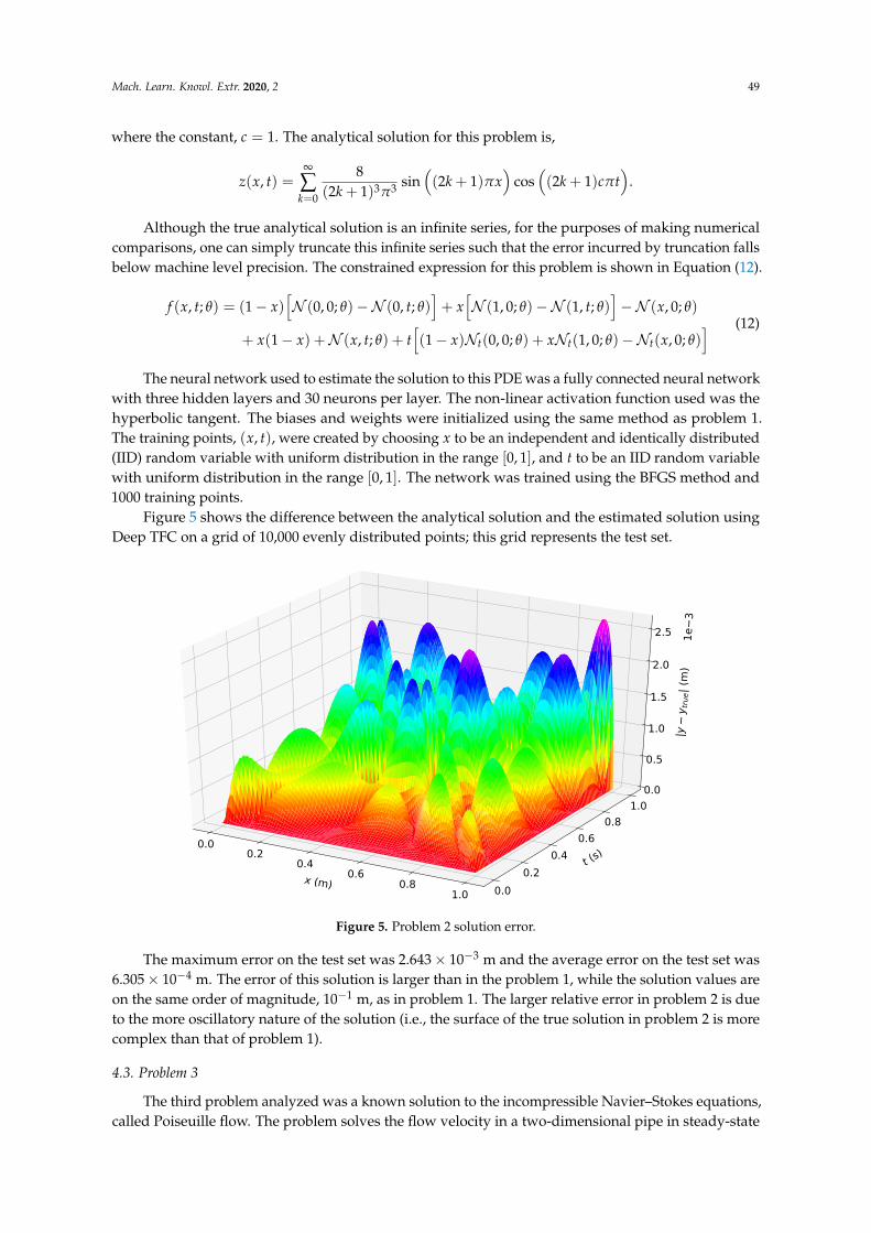
Figure 5 shows the difference between the analytical solution and the estimated solution usingDeep TFC on a grid of 10,000 evenly distributed points; this grid represents the test set.

x (m)

0.00.2

0.40.6

0.81.0

t (s)

0.00.2

0.40.6

0.81.0

|yy t

rue|

(m)

1e3

0.0

0.5

1.0

1.5

2.0

2.5

0.0005

0.0010

0.0015

0.0020

0.0025

Figure 5. Problem 2 solution error.

The maximum error on the test set was 2.643× 10−3 m and the average error on the test set was6.305× 10−4 m. The error of this solution is larger than in the problem 1, while the solution values areon the same order of magnitude, 10−1 m, as in problem 1. The larger relative error in problem 2 is dueto the more oscillatory nature of the solution (i.e., the surface of the true solution in problem 2 is morecomplex than that of problem 1).

4.3. Problem 3

The third problem analyzed was a known solution to the incompressible Navier–Stokes equations,called Poiseuille flow. The problem solves the flow velocity in a two-dimensional pipe in steady-state


with a constant pressure gradient applied in the longitudinal axis. Equation (13) shows the associatedequations and boundary conditions.

∂u∂x

+∂v∂y

= 0

ρ

(∂u∂t

+ u∂u∂x

+ v∂u∂y

)= −∂P

∂x+ µ

(∂2u∂x2 +

∂2u∂y2

)ρ

(∂v∂t

+ u∂v∂x

+ v∂v∂y

)= µ

(∂2v∂x2 +

∂2v∂y2

)subject to:

u(0, y, t) = u(L, y, t) = u(x, y, 0) = 12µ

∂P∂x

(y2 −

(H2

)2)

u(x, H2 , t) = u(x,−H

2 , t) = 0

v(0, y, t) = v(L, y, t) = v(x, y, 0) = 0

v(0, H2 , t) = v(0,−H

2 , t) = 0

(13)

where u and v are velocities in the x and y directions respectively, H is the height of the channel, P isthe pressure, ρ is the density, and µ is the viscosity. For this problem, the values H = 1 m, ρ = 1kg/m3, µ = 1 Pa·s, and ∂P

∂x = −5 N/m3 were chosen. The constrained expressions for the u-velocity,f u(x, y, t; θ), and v-velocity, f v(x, y, t; θ), are shown in Equation (14).

f u(x, y, t; θ) = N (x, y, t; θ)−N (x, y, 0; θ) +L− x

L

(N (0, y, 0; θ)−N (0, y, t; θ)

)

+xL

(N (L, y, 0; θ)−N (L, y, t; θ)

)+

P(

4y2 − H2)

8µ

+1

2HL

((2y− H)

((L− x)N

(0,−H

2, 0; θ

)+ xN

(L,−H

2, 0; θ

)− LN

(x,−H

2, 0; θ

)− (L− x)N

(0,−H

2, t; θ

)+ LN

(x,−H

2, t; θ

)− xN

(L,−H

2, t; θ

))− (H + 2y)

((L− x)N

(0,

H2

, 0; θ)− LN

(x,

H2

, 0; θ)+ xN

(L,

H2

, 0; θ)

− (L− x)N(

0,H2

, t; θ)− xN

(L,

H2

, t; θ)+ LN

(x,

H2

, t; θ)))

f v(x, y, t; θ) = N (x, y, t; θ)−N (x, y, 0; θ) +L− x

L

(N (0, y, 0; θ)−N (0, y, t; θ)

)

+xL

(N (L, y, 0; θ)−N (L, y, t; θ)

)+

12HL

((2y− H)

((L− x)N

(0,−H

2, 0; θ

)+ xN

(L,−H

2, 0; θ

)− LN

(x,−H

2, 0; θ

)− (L− x)N

(0,−H

2, t; θ

)+ LN

(x,−H

2, t; θ

)− xN

(L,−H

2, t; θ

))− (H + 2y)

((L− x)N

(0,

H2

, 0; θ)− LN

(x,

H2

, 0; θ)

+ xN(

L,H2

, 0; θ)− (L− x)N

(0,

H2

, t; θ)− xN

(L,

H2

, t; θ)+ LN

(x,

H2

, t; θ)))

(14)

The neural network used to estimate the solution to this PDE was a fully connected neural networkwith four hidden layers and 30 neurons per layer. The non-linear activation function used was thesigmoid. The biases and weights were initialized using the same method as problem 1. The trainingpoints, (x, y, t), were created by sampling x, y, and t IID from a uniform distribution that spannedthe range of the associated independent variable. For x, the range was [0, 1]. For y, the range was[−H

2 , H2 ], and for t, the range was [0, 1]. The network was trained using the BFGS method on a batch


size of 1000 training points. The loss function used was the sum of the squares of the residuals of thethree PDEs in Equation (13).

The maximum error in the u-velocity was 3.308× 10−7 m per second, the average error in theu-velocity was 9.998× 10−8 m per second, the maximum error in the v-velocity was 5.575× 10−7 m persecond, and the average error in the v-velocity was 1.542× 10−7 m per second. Despite the complexity,the maximum error and average error for this problem are six to seven orders of magnitude lowerthan the solution values. However, the constrained expression for this problem essentially encodes thesolution, because the initial flow condition at time zero is the same as the flow condition throughoutthe spatial domain at any time. Thus, if the neural network outputs a value of zero for all inputs,the problem will be solved exactly. Although the neural network does output a very small value for allinputs, it is interesting to note that none of the layers have weights or biases that are at or near zero.

4.4. Problem 4

The fourth problem is another solution to the Navier–Stokes equations, and is very similar tothe third. The only difference is that in this case, the fluid is not in steady state, it starts from rest.Equation (15) shows the associated equations and boundary conditions.

∂u∂x

+∂v∂y

= 0

ρ

(∂u∂t

+ u∂u∂x

+ v∂u∂y

)= − ∂P

∂x+ µ

(∂2u∂x2 +

∂2u∂y2

)ρ

(∂v∂t

+ u∂v∂x

+ v∂v∂y

)= µ

(∂2v∂x2 +

∂2v∂y2

)subject to:

u(0, y, t) = ∂u∂x (L, y, t) = u(x, y, 0) = 0

u(x, H2 , t) = u(x,− H

2 , t) = 0

v(0, y, t) = ∂v∂x (L, y, t) = v(x, y, 0) = 0

v(x, H2 , t) = v(x,− H

2 , t) = 0

(15)

This problem was created to avoid encoding the solution to the problem into the constrainedexpression, as was the case in the previous problem. The constrained expressions for the u-velocity,f u(x, y, t; θ), and v-velocity, f v(x, y, t; θ), are shown in Equation (16).

f u(x, y, t; θ) = N (x, y, t; θ)−N (x, y, 0; θ) +N (0, y, 0; θ)−N (0, y, t; θ) + xNx(L, y, 0; θ)− xNx(L, y, t; θ)

+1

2H

((2y− H)

(N(

0,−H2

, 0; θ)−N

(x,−H

2, 0; θ

)+ xNx

(L,−H

2, 0; θ

)−N

(0,−H

2, t; θ

)+N

(x,−H

2, t; θ

)− xNx

(L,−H

2, t; θ

))− (H + 2y)

(N(

0,H2

, 0; θ)−N

(x,

H2

, 0; θ)

+ xNx

(L,

H2

, 0; θ)−N

(0,

H2

, t; θ)+N

(x,

H2

, t; θ)− xNx

(L,

H2

, t; θ)))

f v(x, y, t; θ) = N (x, y, t; θ)−N (x, y, 0; θ) +N (0, y, 0; θ)−N (0, y, t; θ) + xNx(L, y, 0; θ)− xNx(L, y, t; θ)

+1

2H

((2y− H)

(N(

0,−H2

, 0; θ)−N

(x,−H

2, 0; θ

)+ xNx

(L,−H

2, 0; θ

)−N

(0,−H

2, t; θ

)+N

(x,−H

2, t; θ

)− xNx

(L,−H

2, t; θ

))− (H + 2y)

(N(

0,H2

, 0; θ)−N

(x,

H2

, 0; θ)

+ xNx

(L,

H2

, 0; θ)−N

(0,

H2

, t; θ)+N

(x,

H2

, t; θ)− xNx

(L,

H2

, t; θ)))

(16)

The neural network used to estimate the solution to this PDE was a fully connected neuralnetwork with four hidden layers and 30 neurons per layer. The non-linear activation function used was


the hyperbolic tangent. The biases and weights were initialized using the same method as problem 1.Problem 4 used 2000 training points that were selected the same way as in problem 3, except the newranges for the independent variables were [0, 15] for x, [0, 3] for t, and [−H

2 , H2 ] for y.

Figures 6–8 show the u-velocity of the fluid throughout the domain at three different times.Qualitatively, the solution should look as follows. The solution should be symmetric about the liney = 0, and the solution should develop spatially and temporally such that after a sufficient amount oftime has passed and sufficiently far from the inlet, x = 0, the u-velocity will be equal, or very nearlyequal, to the steady state u-velocity of problem 3. Qualitatively, the u-velocity field looks correct inFigures 7 and 8, and throughout most of the spatial domain in Figure 6. However, near the left end ofFigure 6, the shape of the highest velocity contour does not match that of the other figures. This stemsfrom the fact that none of the training points fell near this location. Other numerical estimations of thisPDE were made with the exact same method, but with different sets of random training points, and inthose that had training points near this location, the u-velocity matched the qualitative expectation.However, none of those estimated solutions had a quantitative u-velocity with an error as low as theone shown in Figures 6–8. Quantitatively, the u-velocity at x = 15 from Figure 8 was compared withthe known steady state u-velocity, and had a maximum error of 5.378× 10−4 m per second and anaverage error of 3.117× 10−4 m per second.

Figure 6. u-velocity in meters per second at 0.01 s.




5. Conclusions

This article demonstrated how to combine neural networks with the Theory of FunctionalConnections (TFC) into a new methodology, called Deep TFC, that was used to estimate the solutionsof PDEs. Results on this methodology applied to four problems were presented that display howaccurately relatively simple neural networks can approximate the solutions to some well known PDEs.The difficulty of the PDEs in these problems ranged from linear, two-dimensional PDEs to coupled,non-linear, three-dimensional PDEs. Moreover, while the focus of this article was on numericallyestimating the solutions of PDEs, the capability to embed constraints into neural networks has thepotential to positively impact performance when solving any problem that has constraints, not justdifferential equations, with a neural network.

Future work should investigate the performance of different neural network architectures onthe estimated solution error. For example, Ref. [4] suggests a neural network architecture where thehidden layers contain element-wise multiplications and sums of sub-layers. The sub-layers are morestandard neural network layers like the fully connected layers used in the neural networks of thisarticle. Another architecture to investigate is that of extreme learning machines [22]. This architectureis a single layer neural network where the weights of the linear output layer are the only trainableparameters. Consequently, these architectures can ultimately be trained by linear or non-linear leastsquares for linear or non-linear PDEs respectively.

Another topic for investigation is reducing the estimated solution error by sampling the trainingpoints based on the loss function values for the training points of the previous iteration. For example,one could create batches where half of the new batch consists of half of the points in the previous batchthat had the largest loss function value and the other half are randomly sampled from the domain.This should consistently give training points that are in portions of the domain where the estimatedsolution is farthest from the real solution.

Finally, future work will explore extending the hybrid systems approach presented in Ref. [23]to n-dimensions. Doing so would enable Deep TFC to solve problems that involve discontinuitiesat interfaces. For example, consider a heat conduction problem that involves two slabs of differentthermal conductivities in contact with one another. At the interface condition, the temperature iscontinuous but the derivative of temperature is not.

Author Contributions: Conceptualization, C.L.; Formal analysis, C.L.; Methodology, C.L.; Software, C.L.;Supervision, D.M.; Writing—original draft, C.L.; Writing—review & editing, C.L. and D.M. All authors have readand agreed to the published version of the manuscript.

Funding: This work was supported by a NASA Space Technology Research Fellowship, Leake [NSTRF 2019]Grant #: 80NSSC19K1152.


Acknowledgments: The authors would like to acknowledge Jonathan Martinez for valuable advice on neuralnetwork architecture and training methods. In addition, the authors would like to acknowledge Robert Furfaroand Enrico Schiassi for suggesting extreme learning machines as a future work topic. Finally, the authors wouldlike to acknowledge Hunter Johnston for providing computational resources.

Conflicts of Interest: The authors declare no conflict of interest.

Abbreviations

The following abbreviations are used in this manuscript:

FEM finite element methodIID Independent and identically distributedPDE partial differential equationTFC Theory of Functional Connections

References

1. Argyris, J.; Kelsey, S. Energy Theorems and Structural Analysis: A Generalized Discourse with Applicationson Energy Principles of Structural Analysis Including the Effects of Temperature and Non-Linear Stress-StrainRelations. Aircr. Eng. Aerosp. Technol. 1954, 26, 347–356, doi:10.1108/eb032482.

2. Turner, M.J.; Clough, R.W.; Martin, H.C.; Topp, L.J. Stiffness and Deflection Analysis of Complex Structures.J. Aeronaut. Sci. 1956, 23, 805–823, doi:10.2514/8.3664.

3. Clough, R.W. The Finite Element Method in Plane Stress Analysis; American Society of Civil Engineers: Reston,VA, USA, 1960; pp. 345–378.

4. Spiliopoulos, J.S.K. DGM: A deep learning algorithm for solving partial differential equations.J. Comput. Phys. 2018, 1339–1364, doi:10.1016/J.Jcp.2018.08.029.

5. Lagaris, I.E.; Likas, A.; Fotiadis, D.I. Artificial neural networks for solving ordinary and partial differentialequations. IEEE Trans. Neural Netw. 1998, 9, 987–1000, doi:10.1109/72.712178.

6. Yadav, N.; Yadav, A.; Kumar, M. An Introduction to Neural Network Methods for Differential Equations; Springer:Dordrecht, The Netherlands, 2015, doi:10.1007/978-94-017-9816-7.

7. Coons, S.A. Surfaces for Computer-Aided Design of Space Forms; Technical report; Massachusetts Institute ofTechnology: Cambridge, MA, USA, 1967.

8. Mortari, D. The Theory of Connections: Connecting Points. MDPI Math. 2017, 5, 57.9. Mortari, D.; Leake, C. The Multivariate Theory of Connections. MDPI Math. 2019, 7, 296,

doi:10.3390/math7030296.10. Leake, C.; Johnston, H.; Smith, L.; Mortari, D. Analytically Embedding Differential Equation Constraints

into Least Squares Support Vector Machines Using the Theory of Functional Connections. Mach. Learn.Knowl. Extr. 2019, 1, 1058–1083, doi:10.3390/make1040060.

11. Mortari, D. Least-squares Solutions of Linear Differential Equations. MDPI Math. 2017, 5, 48.12. Mortari, D.; Johnston, H.; Smith, L. Least-squares Solutions of Nonlinear Differential Equations.

In Proceedings of the 2018 AAS/AIAA Space Flight Mechanics Meeting Conference, AAS/AIAA, Kissimmee,FL, USA, 8–12 January 2018.

13. Johnston, H.; Mortari, D. Linear Differential Equations Subject to Relative, Integral, and Infinite Constraints.In Proceedings of the 2018 AAS/AIAA Astrodynamics Specialist Conference, Snowbird, UT, USA August19–23, 2018

14. Leake, C.; Mortari, D. An Explanation and Implementation of Multivariate Theory of Connections viaExamples. In Proceedings of the 2019 AAS/AIAA Astrodynamics Specialist Conference, AAS/AIAA,Portland, MN, USA, 11–15 August 2019.

15. Abadi, M.; Agarwal, A.; Barham, P.; Brevdo, E.; Chen, Z.; Citro, C.; Corrado, G.S.; Davis, A.; Dean, J.;Devin, M.; et al. TensorFlow: Large-Scale Machine Learning on Heterogeneous Systems. 2015.Available online: tensorflow.org (accessed on 30 January 2020).

16. Baydin, A.G.; Pearlmutter, B.A.; Radul, A.A. Automatic differentiation in machine learning: A survey.arXiv 2015, arXiv:1502.05767.

17. Kingma, D.P.; Ba, J. Adam: A Method for Stochastic Optimization. arXiv 2014, arXiv:1412.6980.

tensorflow.org


18. Duchi, J.; Hazan, E.; Singer, Y. Adaptive Subgradient Methods for Online Learning and StochasticOptimization. J. Mach. Learn. Res. 2011, 12, 2121–2159.

19. Tieleman, T.; Hinton, G. Lecture 6.5—RMSProp, COURSERA: Neural Networks for Machine Learning; Technicalreport; University of Toronto: Toronto, ON, Canada, 2012.

20. Fletcher, R. Practical Methods of Optimization, 2nd ed.; Wiley: New York, NY, USA, 1987.21. Glorot, X.; Bengio, Y. Understanding the difficulty of training deep feedforward neural networks.

In Proceedings of the Thirteenth International Conference on Artificial Intelligence and Statistics, Sardinia,Italy, 13–15 May 2010; Teh, Y.W., Titterington, M., Eds.; PMLR: Sardinia, Italy, 2010; Volume 9, pp. 249–256.

22. Huang, G.B.; Zhu, Q.Y.; Siew, C.K. Extreme learning machine: Theory and applications . Neurocomputing2006, 70, 489–501, doi:10.1016/j.neucom.2005.12.126.

23. Johnston, H.; Mortari, D. Least-squares solutions of boundary-value problems in hybrid systems. arXiv 2019,arXiv:1911.04390.

c© 2020 by the authors. Licensee MDPI, Basel, Switzerland. This article is an open accessarticle distributed under the terms and conditions of the Creative Commons Attribution(CC BY) license (http://creativecommons.org/licenses/by/4.0/).

http://creativecommons.org/

http://creativecommons.org/licenses/by/4.0/.

Deep Theory of Functional Connections: A New Method for ...

Documents

Transcript of Deep Theory of Functional Connections: A New Method for ...