Deep Quantization: Encoding Convolutional Activationswith Deep Generative Model ∗

Zhaofan Qiu, Ting Yao, and Tao MeiUniversity of Science and Technology of China, Hefei, China

Microsoft Research, Beijing, China

zhaofanqiu@gmail.com, {tiyao, tmei}@microsoft.com

Abstract

Deep convolutional neural networks (CNNs) haveproven highly effective for visual recognition, where learn-ing a universal representation from activations of convolu-tional layer plays a fundamental problem. In this paper,we present Fisher Vector encoding with Variational Auto-Encoder (FV-VAE), a novel deep architecture that quan-tizes the local activations of convolutional layer in a deepgenerative model, by training them in an end-to-end man-ner. To incorporate FV encoding strategy into deep genera-tive models, we introduce Variational Auto-Encoder model,which steers a variational inference and learning in a neu-ral network which can be straightforwardly optimized us-ing standard stochastic gradient method. Different from theFV characterized by conventional generative models (e.g.,Gaussian Mixture Model) which parsimoniously fit a dis-crete mixture model to data distribution, the proposed FV-VAE is more flexible to represent the natural property of da-ta for better generalization. Extensive experiments are con-ducted on three public datasets, i.e., UCF101, ActivityNet,and CUB-200-2011 in the context of video action recogni-tion and fine-grained image classification, respectively. Su-perior results are reported when compared to state-of-the-art representations. Most remarkably, our proposed FV-VAE achieves to-date the best published accuracy of 94.2%on UCF101.

1. IntroductionThe recent advances in deep convolutional neural net-

works (CNNs) have demonstrated high capability in visu-al recognition. For instance, an ensemble of residual net-s [7] achieves 3.57% in terms of top-5 error on the Ima-geNet dataset [26]. More importantly, when utilizing theactivations of either a fully-connected layer or a convolu-

∗This work was performed when Zhaofan Qiu was visiting Mi-crosoft Research as a research intern.

......

...

...

Global Activations

ConvolutionalActivations

FV Encoding

FV-VAE Encoding

ConvolutionalActivations

Figure 1. Visual representations derived from activations of dif-ferent layers in CNNs (upper row: global activations of the fully-connected layer; middle row: convolutional activations with Fish-er Vector encoding; bottom row: convolutional activations withour FV-VAE encoding).

tional layer in a pre-trained CNN as a universal visual rep-resentation and applying this representation to other visu-al recognition tasks (e.g., scene understanding and seman-tic segmentation), CNNs also manifest impressive perfor-mances. The improvements are expected when CNNs arefurther fine-tuned with only amount of task-specific data.

The activations of different layers in CNNs are generallygrouped into two dimensions: global activations and con-volutional activations. The former directly takes the activa-tions of the fully-connected layer as visual representations,which are holistic over the entire image, as shown in theupper row of Figure 1. The latter, in contrast, creates vi-sual representations by encoding a set of regional and localactivations from a convolutional layer to a vectorial repre-sentation using quantization strategies. For example, FisherVector (FV) [23] is one of the most successful quantizationapproaches, as shown in the middle row of Figure 1. Whilesuperior results by aggregating convolutional activations arereported in most recent studies [3, 44], convolutional acti-vations are first extracted as local descriptors followed byanother separate quantization step. Thus such descriptorsmay not be optimally compatible with the encoding pro-cess, making the quantization sub-optimal. Furthermore, as

discussed in [13], the generative model behind FV, i.e., theGaussian Mixture Model (GMM), cannot always represen-t the natural clustering of the descriptors and its inflexibleGaussian observation model limits its generalization ability.

We show in this paper that these two limitations can bemitigated by designing a deep architecture for representa-tion learning that combines convolutional activations ex-traction and quantization into a one-stage learning. Specif-ically, we present a novel Fisher Vector encoding withVariational Auto-Encoder (FV-VAE) framework to encodeconvolutional activations with deep generative model (i.e.,VAE), as shown in the bottom row of Figure 1. The pipelineof the proposed deep architecture generally consists of twocomponents: a sub-network with a stack of convolution lay-ers to produce convolutional activations followed by a VAEstructure aggregating the regional convolutional descriptorsto a FV. VAE consists of hierarchies of conditional stochas-tic variables and is a highly expressive model by optimizinga variational approximation (an inference/recognition mod-el) to the intractable posterior for the generative distribution.Compared to traditional GMM model which has the form ofa mixture of fixed Gaussian components, the inference mod-el here can be regarded as an alternative to predict specificGaussian components to different inputs by a single neuralnetwork, making it more flexible. It is also worth noting thata classification loss is additionally considered to preservethe semantic information in the training stage. The entirearchitecture is trainable in an end-to-end fashion. Further-more, in the feature extraction stage, we theoretically provethat the FV of input descriptors can be directly computedby accumulating the gradient vector of reconstruction lossin the VAE through back-propagation.

The main contribution of this work is the proposal of FV-VAE architecture to encode convolutional descriptors withVariational Auto-Encoder. We theoretically formulate thecomputation of FV in VAE and substantiate an implemen-tation of FV-VAE for visual representation learning.

2. Related WorkIn the literature, visual representation generation from a

pre-trained CNN model has proceeded along two dimen-sions: global activations and convolutional activations. Thefirst is to extract visual representation from global acti-vations in a CNN directly, e.g., the outputs from fully-connected layer in VGG [30] or pool5 layer in ResNet [7].In practice, this scheme often starts by pre-training CNNmodel on a large dataset (e.g., ImageNet) and then fine-tuning the CNN architecture with a small amount of task-specific data to better characterize the intrinsic informa-tion in target scenario. The visual representation learnt inthis direction has been exploited in a broad range of com-puter vision tasks including fine-grained image classifica-tion [1, 17], video action recognition [18, 19, 24, 29] and

visual captioning [36, 38].Another alternative scheme is to utilize the activation-

s from convolutional layers in CNN as regional and localdescriptors. Compared to global activations, convolutionalactivations from CNN are embedded with rich spatial in-formation, making them more transferable to different do-mains and more robust to translation and rotation, whichhave shown the effectiveness in several technological ad-vances, e.g., Spatial Pyramid Pooling (SPP) [6], Fast R-CNN [5] and Fully Convolutional Networks (FCNs) [22].Recently, many works attempt to produce visual represen-tation by encoding convolutional activations with differentquantization strategies. For example, Fisher Vector [23] iscomputed on the output of the last convolutional layer ofVGG networks for describing texture in [3]. Similar in spir-it, Xu et al. utilize VLAD [11] to encode convolutionaldescriptors of video frame for multimedia event detection[44]. In [28] and [43], Sharma et al. and Xu et al. dynam-ically pool convolutional descriptors with attention modelsfor action recognition and image captioning, respectively.Furthermore, convolutional descriptors of one convolution-al layer are pooled with the guidance of the activations ofthe successive convolutional layer in [21]. In [20], convolu-tional descriptors from two CNNs are multiplied using theouter product and pooled to obtain the bilinear vector.

In summary, our work belongs to the second dimen-sion and aims to compute FV on convolutional activationswith deep generative models. We exploit Variational Auto-Encoder for this purpose, which optimizes an inferencemodel to the intractable posterior. The high flexibility ofthe inference model and efficiency of the structure optimiza-tion makes VAE more advanced than traditional GMM. Ourwork in this paper contributes by studying not only encod-ing convolutional activations in a deep architecture, but alsotheoretically figuring out the computation of FV based onVAE architecture.

3. Fisher Vector Meets VAEIn this section, we first recall the Fisher Vector theory,

followed by presenting how to estimate the probability den-sity function in FV through VAE. The optimization of VAEis then elaborated and how to compute the FV of the inputdescriptors will be introduced finally.

3.1. Fisher Vector Theory

Suppose we have two sets of local descriptors X =

{xt}Txt=1 and Y = {yt}

Ty

t=1 with Tx and Ty descriptors, re-spectively. Let xt,yt ∈ Rd denote the d-dimensional fea-tures of each descriptor. In order to measure the similaritybetween the two sets, kernel method is employed by map-ping them into a hyperspace. Specifically, assuming thatthe generation process of descriptors in Rd can be mod-eled by a probability density function uθ with M param-

...

ReconstructionLoss

... RegularizationLoss

ClassificationLoss

...

...

Encoder Sampling Decoder

(a) VAE Training

... ReconstructionLoss

...

...

...

Encoder Identity Decoder

Back Propagation

Gradient VectorAccumulator

(b) FV Extraction

Figure 2. The overview of FV learning with VAE: (a) The trainingprocess of VAE, (b) FV extraction based on VAE.

eters θ = [θ1, ..., θM ]′, Fisher Kernel (FK) [9] between thetwo sets X and Y is given by

K(X,Y ) = GXθ

′F−1θ GY

θ , (1)

where GXθ = ∇θ log uθ(X) is defined as fisher score

function by computing the gradient of the log-likelihoodof the set based on the generative model, and Fθ =EX∼uθ

[GXθ G

Xθ

′] is the Fisher Information Matrix (FIM) of

uθ which is regarded as statistical feature normalization. S-ince Fθ is positive semi-definite, the FK in Eq.(1) can bere-written explicitly as inner product in hyperspace:

K(X,Y ) = G Xθ

′G Yθ , (2)

where

G Xθ = F

− 12

θ GXθ = F

− 12

θ ∇θ log uθ(X) . (3)

Formally, G Xθ is well-known as Fisher Vector (FV). The

dimension of FV is equal to the number of generative pa-rameters θ, which is often much higher than that of the de-scriptor, making FV of higher descriptive capability.

3.2. Probability Estimation through VAE

Next, we will discuss how to estimate the probabilitydensity function uθ in FV. In general, uθ is chosen to beGaussian Mixture Model (GMM) [27, 40] as one can ap-proximate any distribution with arbitrary precision by GM-M, in which θ is composed of mixture weight, mean and co-variance of Gaussian components. The need of a large num-ber of mixture components and inefficient optimization ofExpectation Maximization algorithm, however, makes theparameter learning computationally expensive and difficultto be applied to large-scale complex data. Inspired by theidea of deep generative models [16, 25] which enable theflexible and efficient inference learning in a neural network,

Algorithm 1 Variational Auto-Encoding (VAE) Optimization

1: Input: training set X = {xt}Txt=1, corresponding labels L =

{lt}Txt=1, loss weights λ1, λ2, λ3.

2: Initialization: random initialized θ0,φ0.3: Output: VAE parameters θ∗,φ∗.4: repeat5: Sample xt in the minibatch.6: Encoder: µzt

← fφ(xt).7: Sampling: zt ← µzt

+ ε� σz, ε ∼ N (0, I).8: Decoder: µxt

← fθ(zt).9: Compute reconstruction loss:

Lrec = − log pθ(xt|zt) = − logN (xt;µxt,σ2

xI).10: Compute regularization loss:

Lreg = 12

∥∥µzt

∥∥+ 12‖σz‖ − 1

2

∑dk=1(1 + log σ2

z(k)).11: Compute classification loss:

Lcls = softmax loss(zt, lt).12: Fuse the three loss:

L(θ,φ) = λ1Lrec(θ,φ) + λ2Lreg(φ) + λ3Lcls(φ).13: Back-propagate the gradients.14: until maximum iteration reached.

we develop a Variational Auto-Encoder (VAE) to generatethe probability function uθ.

Following the notations in Section 3.1 and assumingthat all the descriptors in the set are independent, the log-likelihood of the set can be calculated by the sum over log-likelihoods of individual descriptor and written as

log uθ(X) =

Tx∑t=1

log pθ(xt) . (4)

To model the probability of xt generated from parame-ters θ, an unobserved continuous random variable zt is in-volved with prior distribution pθ(z) and each xt is generat-ed from the conditional distribution pθ(x|z). As such, eachlog-likelihood log pθ(xt) can be measured using Kullback-Leibler divergence (DKL) as

log pθ(xt) = DKL(qφ(z|xt)||pθ(z|xt)) + LB(θ,φ;xt)

> LB(θ,φ;xt), (5)

where LB(θ,φ;xt) is the variational lower bound on thelikelihood of descriptor xt and can be written as

LB(θ,φ;xt) = −DKL(qφ(z|xt)||pθ(z))+Eqφ(z|xt)[log pθ(xt|z)],(6)

where qφ(z|x) is a recognition model which is an approxi-mation to the intractable posterior pθ(z|x). In our proposedFV-VAE method, we use this lower bound LB(θ,φ;xt) asan approximation of the log-likelihood. Through this ap-proximation, the generative model can be divided into t-wo parts: encoder qφ(z|x) and decoder pθ(x|z), predictinghidden and visible probability, respectively.

FV-VAE

GradientVector

VisualRepresentation

Loss Function

Ice Dancing/Albatross

+

Training Epoch

Extraction Epoch

CNN

CNN

ConvolutionalActivations

LocalFeature Set

SPP

224x224

448x448

50/frame

ConvolutionalActivations

Denser Grid (28x28)

784/image

Video Classification

Image Classification

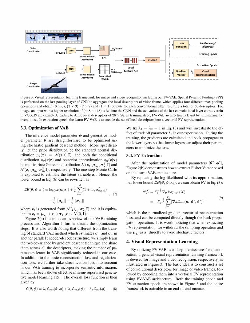
Figure 3. Visual representation learning framework for image and video recognition including our FV-VAE. Spatial Pyramid Pooling (SPP)is performed on the last pooling layer of CNN to aggregate the local descriptors of video frame, which applies four different max poolingoperations and obtain (6 × 6), (3 × 3), (2 × 2) and (1 × 1) outputs for each convolutional filter, resulting a total of 50 descriptors. Forimage, an input with a higher resolution of (448× 448) is fed into the CNN and the activations of the last convolutional layer conv5 4+reluin VGG 19 are extracted, leading to dense local descriptors of 28× 28. In training stage, FV-VAE architecture is learnt by minimizing theoverall loss. In extraction epoch, the learnt FV-VAE is to encode the set of local descriptors into a vectorial FV representation.

3.3. Optimization of VAE

The inference model parameter φ and generative mod-el parameter θ are straightforward to be optimized us-ing stochastic gradient descend method. More specifical-ly, let the prior distribution be the standard normal dis-tribution pθ(z) = N (z; 0, I), and both the conditionaldistribution pθ(x|z) and posterior approximation qφ(z|x)be multivariate Gaussian distributionN (xt;µxt

,σ2xtI) and

N (zt;µzt,σ2

ztI), respectively. The one-step Monte Carlo

is exploited to estimate the latent variable zt. Hence, thelower bound in Eq. (6) can be rewritten as

LB(θ,φ;xt) ' log pθ(xt|zt) +1

2

d∑k=1

(1 + log σ2zt(k))

− 1

2

∥∥µzt

∥∥− 1

2‖σzt‖

, (7)

where zt is generated from N (µzt,σ2

ztI) and it is equiva-

lent to zt = µzt+ ε� σzt

,ε ∼ N (0, I).Figure 2(a) illustrates an overview of our VAE training

process and Algorithm 1 further details the optimizationsteps. It is also worth noting that different from the train-ing of standard VAE method which estimates σx and σz inanother parallel encoder-decoder structure, we simply learnthe two covariance by gradient descent technique and sharethem across all the descriptors, making the number of pa-rameters learnt in VAE significantly reduced in our case.In addition to the basic reconstruction loss and regulariza-tion loss, we further take classification loss into accountin our VAE training to incorporate semantic information,which has been shown effective in semi-supervised genera-tive model learning [15]. The overall loss function is thengiven by

L(θ,φ) = λ1Lrec(θ,φ) + λ2Lreg(φ) + λ3Lcls(φ) . (8)

We fix λ1 = λ2 = 1 in Eq. (8) and will investigate the ef-fect of tradeoff parameter λ3 in our experiments. During thetraining, the gradients are calculated and back-propagate tothe lower layers so that lower layers can adjust their param-eters to minimize the loss.

3.4. FV Extraction

After the optimization of model parameters [θ∗,φ∗],Figure 2(b) demonstrates how to extract Fisher Vector basedon the learnt VAE architecture.

By replacing the log-likelihood with its approximation,i.e., lower boundLB(θ,φ;xt), we can obtain FV in Eq. (3):

G Xθ∗ = F

− 12

θ∗ ∇θ log uθ∗(X)

= −F−12

θ∗

Tx∑t=1

[∇θLrec(xt;θ∗,φ∗)]

, (9)

which is the normalized gradient vector of reconstructionloss, and can be computed directly though the back propa-gation operation. It is worth noticing that when extractingFV representation, we withdraw the sampling operation anduse µzt

as zt directly to avoid stochastic factors.

4. Visual Representation LearningBy utilizing FV-VAE as a deep architecture for quanti-

zation, a general visual representation learning frameworkis devised for image and video recognition, respectively, asillustrated in Figure 3. The basic idea is to construct a setof convolutional descriptors for image or video frames, fol-lowed by encoding them into a vectorial FV representationusing FV-VAE architecture. Both the training epoch andFV extraction epoch are shown in Figure 3 and the entireframework is trainable in an end-to-end manner.

We exploit different strategies of aggregation to con-struct the set of convolutional descriptors for video framesand image, respectively, due to the different property in be-tween. A video consists of a sequence of frames with largeintra-class variations caused by, e.g., camera motion, illu-mination conditions and so on, making the scale of an i-dentical object varying in different frames. Following [44],we employ Spatial Pyramid Pooling (SPP) [6] on the lastpooling layer to extract scale-invariant local descriptors forvideo frames. Instead, we feed a higher resolution (e.g.,448× 448) input into the CNN to fully utilize image infor-mation and extract the activations of the last convolutionallayer (e.g., conv5 4+relu in VGG 19), resulting in dense lo-cal descriptors (e.g., 28× 28) for image as in [20].

In our implementation, Multi-Layer Perceptron (MLP)is employed as encoder and decoder in FV-VAE and onelayer decoder is developed to reduce the dimension of FVrepresentation. As such, the functions in Algorithm 1 canbe specified as

Encoder : µzt←MLPφ(xt)

Decoder : µxt← ReLU(W ′θzt + bθ)

, (10)

where {Wθ, bθ} are the encoder parameters θ. The gradi-ent vector of Lrec is calculated as

∇θLrec(xt;θ∗,φ∗) = flatten

{[∂Lrec

∂Wφ,∂Lrec

∂bθ]

}= flatten

{[∂Lrec

∂µxt

· z′t,∂Lrec

∂µxt

]

}= flatten

{∂Lrec

∂µxt

· [z′t, 1]}

= flatten

{µxt− xt

σ2x

� (µxt> 0) · [z′t, 1]

},

(11)where “flatten” represents to flatten a matrix to a vector,and � denotes element-wise multiplication to filter the ac-tivated elements. Considering it is difficult to obtain an an-alytic solution of FIM in this case, we make an approxima-tion by replacing the expectation with the average on thewhole training set:

Fθ∗ = EX∼uθ [GXθ G

Xθ

′] ≈ mean

X[GX

θ GXθ

′] , (12)

and

G Xθ∗ = flatten

{−F−

12

θ∗ ·Tx∑t=1

(µxt− xt

σ2x

� (µxt> 0) · [z′t, 1])

},

(13)which is the output FV representation in our framework.

To improve the convergence speed and better regularizethe visual representation learning for video, we train thisframework by inputting one single video frame rather thanmultiple ones, which is randomly sampled from videos. Inthe FV extraction stage, the video-level representation can

Table 1. Methodology comparison of different quantization.Quantization indicator descriptorFV [23] Gaussian observation

modelgradient with respect toGMM parameters

VLAD [11] clustering center difference to the as-signed center

BP [20] local feature coordinate representa-tion

FV-VAE VAE hidden variable gradient of reconstruc-tion loss

be easily obtained by averaging FVs of all the frames sam-pled from the video since FV in Eq. (13) is linear additive.

5. ExperimentsWe evaluate the learnt visual representation by FV-VAE

architecture on three popular datasets, i.e., UCF101 [31],ActivityNet [2] and CUB-200-2011 [39]. The UCF101dataset is one of the most popular video action recogni-tion benchmarks. It consists of 13,320 videos from 101action categories. The action categories are divided intofive groups: human-object interaction, body-motion only,human-human interaction, playing musical instruments andsports. Three training/test splits are provided by the datasetorganisers and each split in UCF101 includes about 9.5Ktraining and 3.7K test videos. The ActivityNet dataset isa large-scale video benchmark for human activity under-standing. The latest released version of the dataset (v1.3)is exploited, which contains 19,994 videos from 200 activ-ity categories. The 19,994 videos are divided into 10,024,4,926, 5,044 videos for training, validation and test set, re-spectively. Note that the labels of test set are not publiclyavailable and the performances on ActivityNet dataset areall reported on validation set. Furthermore, we also val-idate the representation on CUB-200-2011 dataset, whichis widely adopted for fine-grained image classification andconsists of 11,788 images from 200 bird species. We fol-low the official split on this dataset with 5,994 training and5,794 test images.

5.1. Compared Approaches

To empirically verify the merit of visual representationlearnt by FV-VAE, we compare the following quantizationmethods: Global Activations (GA) directly utilizes theoutputs of fully-connected/pooling layer as visual represen-tation. Fisher Vector (FV) [23] produces the visual repre-sentation by concatenating the gradients with respect to theparameters of GMM, which is trained on local descriptors.Vector of Locally Aggregated Descriptors (VLAD) [11]is to accumulate, for each clustering center learnt with K-means, the differences between the clustering center and thedescriptors assigned to it, and then concatenates the accu-mulated vector of each center as quantized representation.

Bilinear Pooling (BP) [20] pools local descriptors in a pair-wise manner by outer product. In our case, one local de-scriptor pairs with itself. To better illustrate the differencebetween the compared approaches, we details the methodol-ogy in Table 1. In particular, we decouple the quantizationprocess into two parts: indicator and descriptor. Indicatorrefers to observations/distributions estimated on the wholeset of local descriptors and descriptor is to represent the setwith respect to the indicator.

5.2. Experimental Settings

Convolutional activations. On video action recognitiontask, we extract two widely adopted convolutional activa-tions, i.e., activations of pool5 layer in VGG 19 [30] andres5c layer in ResNet 152 [7]. Given a 224 × 224 videoframe as input, the outputs of the two layers are both 7× 7and the dimension of each activation is 512 and 2,048, re-spectively. For each video, 25 frames are uniformly sam-pled for representation extraction. On image classificationproblem, we feed 448×448 image into VGG 19 and the ac-tivations of conv5 4+relu layer are exploited, which produce28× 28 convolutional descriptors.

VAE optimization. To make the training process ofVAE stable, we first exploit L2 normalization on each con-volutional activation to make the input to VAE in a com-mon scale. Following [8, 37], dropout is then employed torandomly drop out units input to the encoder but the auto-encoder is optimized to reconstruct a complete “repaired”input. The dropout rate is fixed to 0.5. Furthermore, weutilize AdaDelta [46] optimization method implemented inCaffe [12] to normalize the gradient of each parameters forbalancing their converge speed. The base learning rate is setto 1 and the size of mini-batch is 128 images/frames. Theoptimization will be complete after 5,000 batches.

Quantization settings. For our FV-VAE, given the lo-cal descriptor with dimension C (C ∈ {512, 2048}), wedesign a two-layer encoder (C → C → 255) to reducethe dimension to 255, coupled with a single layer decoder(255 → C). The dimension of the final quantized repre-sentation is 256 × C. For FV and VLAD, we follow thesettings in [3] and [44]. Specifically, 128 Gaussian com-ponents for FV and 256 clustering centers for VLAD areexploited. As such, the dimension of representations en-coded by FV and VLAD will also be 256 × C. The twoquantization approaches are implemented by VLFeat [35].

Classifier training. After representation learning by allthe methods in our experiments, we apply signed square-root step (sign(x)

√|x|) and L2 normalization (x/‖x‖2) as

in [3, 20, 23, 44], and then train a one-vs-all linear SVMwith a fixed hyperparameter Csvm = 100.

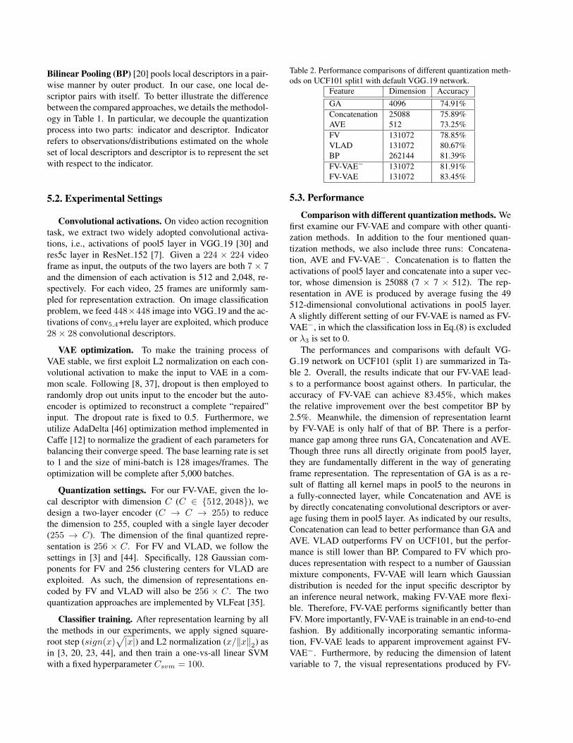
Table 2. Performance comparisons of different quantization meth-ods on UCF101 split1 with default VGG 19 network.

Feature Dimension AccuracyGA 4096 74.91%Concatenation 25088 75.89%AVE 512 73.25%FV 131072 78.85%VLAD 131072 80.67%BP 262144 81.39%FV-VAE− 131072 81.91%FV-VAE 131072 83.45%

5.3. Performance

Comparison with different quantization methods. Wefirst examine our FV-VAE and compare with other quanti-zation methods. In addition to the four mentioned quan-tization methods, we also include three runs: Concatena-tion, AVE and FV-VAE−. Concatenation is to flatten theactivations of pool5 layer and concatenate into a super vec-tor, whose dimension is 25088 (7 × 7 × 512). The rep-resentation in AVE is produced by average fusing the 49512-dimensional convolutional activations in pool5 layer.A slightly different setting of our FV-VAE is named as FV-VAE−, in which the classification loss in Eq.(8) is excludedor λ3 is set to 0.

The performances and comparisons with default VG-G 19 network on UCF101 (split 1) are summarized in Ta-ble 2. Overall, the results indicate that our FV-VAE lead-s to a performance boost against others. In particular, theaccuracy of FV-VAE can achieve 83.45%, which makesthe relative improvement over the best competitor BP by2.5%. Meanwhile, the dimension of representation learntby FV-VAE is only half of that of BP. There is a perfor-mance gap among three runs GA, Concatenation and AVE.Though three runs all directly originate from pool5 layer,they are fundamentally different in the way of generatingframe representation. The representation of GA is as a re-sult of flatting all kernel maps in pool5 to the neurons ina fully-connected layer, while Concatenation and AVE isby directly concatenating convolutional descriptors or aver-age fusing them in pool5 layer. As indicated by our results,Concatenation can lead to better performance than GA andAVE. VLAD outperforms FV on UCF101, but the perfor-mance is still lower than BP. Compared to FV which pro-duces representation with respect to a number of Gaussianmixture components, FV-VAE will learn which Gaussiandistribution is needed for the input specific descriptor byan inference neural network, making FV-VAE more flexi-ble. Therefore, FV-VAE performs significantly better thanFV. More importantly, FV-VAE is trainable in an end-to-endfashion. By additionally incorporating semantic informa-tion, FV-VAE leads to apparent improvement against FV-VAE−. Furthermore, by reducing the dimension of latentvariable to 7, the visual representations produced by FV-

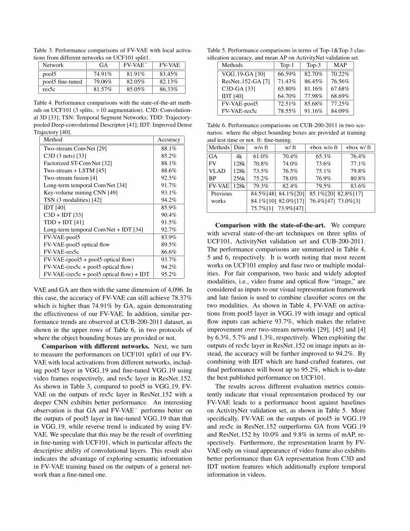
Table 3. Performance comparisons of FV-VAE with local activa-tions from different networks on UCF101 split1.

Network GA FV-VAE− FV-VAEpool5 74.91% 81.91% 83.45%pool5 fine-tuned 79.06% 82.05% 82.13%res5c 81.57% 85.05% 86.33%

Table 4. Performance comparisons with the state-of-the-art meth-ods on UCF101 (3 splits, ×10 augmentation). C3D: Convolution-al 3D [33]; TSN: Temporal Segment Networks; TDD: Trajectory-pooled Deep-convolutional Descriptor [41]; IDT: Improved DenseTrajectory [40].

Method AccuracyTwo-stream ConvNet [29] 88.1%C3D (3 nets) [33] 85.2%Factorized ST-ConvNet [32] 88.1%Two-stream + LSTM [45] 88.6%Two-stream fusion [4] 92.5%Long-term temporal ConvNet [34] 91.7%Key-volume mining CNN [49] 93.1%TSN (3 modalities) [42] 94.2%IDT [40] 85.9%C3D + IDT [33] 90.4%TDD + IDT [41] 91.5%Long-term temporal ConvNet + IDT [34] 92.7%FV-VAE-pool5 83.9%FV-VAE-pool5 optical flow 89.5%FV-VAE-res5c 86.6%FV-VAE-(pool5 + pool5 optical flow) 93.7%FV-VAE-(res5c + pool5 optical flow) 94.2%FV-VAE-(res5c + pool5 optical flow) + IDT 95.2%

VAE and GA are then with the same dimension of 4,096. Inthis case, the accuracy of FV-VAE can still achieve 78.37%which is higher than 74.91% by GA, again demonstratingthe effectiveness of our FV-VAE. In addition, similar per-formance trends are observed at CUB-200-2011 dataset, asshown in the upper rows of Table 6, in two protocols ofwhere the object bounding boxes are provided or not.

Comparison with different networks. Next, we turnto measure the performances on UCF101 split1 of our FV-VAE with local activations from different networks, includ-ing pool5 layer in VGG 19 and fine-tuned VGG 19 usingvideo frames respectively, and res5c layer in ResNet 152.As shown in Table 3, compared to pool5 in VGG 19, FV-VAE on the outputs of res5c layer in ResNet 152 with adeeper CNN exhibits better performance. An interestingobservation is that GA and FV-VAE− performs better onthe outputs of pool5 layer in fine-tuned VGG 19 than thatin VGG 19, while reverse trend is indicated by using FV-VAE. We speculate that this may be the result of overfittingin fine-tuning with UCF101, which in particular affects thedescriptive ability of convolutional layers. This result alsoindicates the advantage of exploring semantic informationin FV-VAE training based on the outputs of a general net-work than a fine-tuned one.

Table 5. Performance comparisons in terms of Top-1&Top-3 clas-sification accuracy, and mean AP on ActivityNet validation set.

Methods Top-1 Top-3 MAPVGG 19-GA [30] 66.59% 82.70% 70.22%ResNet 152-GA [7] 71.43% 86.45% 76.56%C3D-GA [33] 65.80% 81.16% 67.68%IDT [40] 64.70% 77.98% 68.69%FV-VAE-pool5 72.51% 85.68% 77.25%FV-VAE-res5c 78.55% 91.16% 84.09%

Table 6. Performance comparisons on CUB-200-2011 in two sce-narios: where the object bounding boxes are provided at trainingand test time or not. ft: fine-tuning.Methods Dim w/o ft w/ ft +box w/o ft +box w/ ftGA 4k 61.0% 70.4% 65.3% 76.4%FV 128k 70.8% 74.0% 73.6% 77.1%VLAD 128k 73.5% 76.5% 75.1% 79.8%BP 256k 75.2% 78.0% 76.9% 80.8%FV-VAE 128k 79.3% 82.4% 79.5% 83.6%Previousworks

84.5%[48] 84.1%[20]84.1%[10] 82.0%[17]75.7%[1] 73.9%[47]

85.1%[20] 82.8%[17]76.4%[47] 73.0%[3]

Comparison with the state-of-the-art. We comparewith several state-of-the-art techniques on three splits ofUCF101, ActivityNet validation set and CUB-200-2011.The performance comparisons are summarized in Table 4,5 and 6, respectively. It is worth noting that most recentworks on UCF101 employ and fuse two or multiple modal-ities. For fair comparison, two basic and widely adoptedmodalities, i.e., video frame and optical flow “image,” areconsidered as inputs to our visual representation frameworkand late fusion is used to combine classifier scores on thetwo modalities. As shown in Table 4, FV-VAE on activa-tions from pool5 layer in VGG 19 with image and opticalflow inputs can achieve 93.7%, which makes the relativeimprovement over two-stream networks [29], [45] and [4]by 6.3%, 5.7% and 1.3%, respectively. When exploiting theoutputs of res5c layer in ResNet 152 on image inputs as in-stead, the accuracy will be further improved to 94.2%. Bycombining with IDT which are hand-crafted features, ourfinal performance will boost up to 95.2%, which is to-datethe best published performance on UCF101.

The results across different evaluation metrics consis-tently indicate that visual representation produced by ourFV-VAE leads to a performance boost against baselineson ActivityNet validation set, as shown in Table 5. Morespecifically, FV-VAE on the outputs of pool5 in VGG 19and res5c in ResNet 152 outperforms GA from VGG 19and ResNet 152 by 10.0% and 9.8% in terms of mAP, re-spectively. Furthermore, the representation learnt by FV-VAE only on visual appearance of video frame also exhibitsbetter performance than GA representation from C3D andIDT motion features which additionally explore temporalinformation in videos.

12 13 14 15 16 17

Feature dimension (log2)

72

74

76

78

80

82

84

Perc

enta

ge o

n a

ccura

cy

VLAD

FV

FV-VAE¡

FV-VAE

(a)

0 1 2 3 4 5

¸3 in Eq. (8) (log10)

81

82

83

84

85

86

87

88

Perc

enta

ge o

n a

ccura

cy

pool5

pool5 fine-tuned

res5c

(b)

1213141516

Feature dimension (log2)

77

78

79

80

81

82

83

84

85

Perc

enta

ge o

n a

ccura

cy

RM

Latent Variable Reduction

PCA

(c)

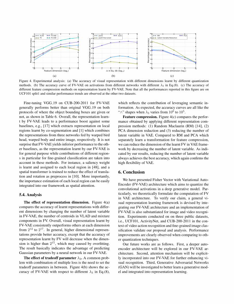
Figure 4. Experimental analysis: (a) The accuracy of visual representation with different dimensions learnt by different quantizationmethods. (b) The accuracy curve of FV-VAE on activations from different networks with different λ3 in Eq.(8). (c) The accuracy ofdifferent feature compression methods on representation learnt by FV-VAE. Note that all the performances reported in this figure are onUCF101 split1 and similar performance trends are observed at the other two datasets.

Fine-tuning VGG 19 on CUB-200-2011 for FV-VAEgenerally performs better than original VGG 19 on bothprotocols of where the object bounding boxes are given ornot, as shown in Table 6. Overall, the representation learn-t by FV-VAE leads to a performance boost against somebaselines, e.g., [17] which extracts representation on localregions learnt by co-segmentation and [1] which combinesthe representations from three networks fed by warped birdhead, warped body and entire image, respectively. It is notsurprise that FV-VAE yields inferior performance to the oth-er baselines, as the representation learnt by our FV-VAE isfor general purpose while contributions of different region-s in particular for fine-grained classification are taken intoaccount in these methods. For instance, a saliency weightis learnt and assigned to each local region in [48], and aspatial transformer is trained to reduce the effect of transla-tion and rotation as preprocess in [10]. More importantly,the importance estimation of each local region can be easilyintegrated into our framework as spatial attention.

5.4. Analysis

The effect of representation dimension. Figure 4(a)compares the accuracy of learnt representations with differ-ent dimensions by changing the number of latent variablein FV-VAE, the number of centroids in VLAD and mixturecomponents in FV. Overall, visual representation learnt byFV-VAE consistently outperforms others at each dimensionfrom 212 to 217. In general, higher dimensional represen-tations provide better accuracy, except that the accuracy ofrepresentation learnt by FV will decrease when the dimen-sion is higher than 215, which may caused by overfitting.The result basically indicates the advantage of predictingGaussian parameters by a neural network in our FV-VAE.

The effect of tradeoff parameter λ3. A common prob-lem with combination of multiple loss is the need to set thetradeoff parameters in between. Figure 4(b) shows the ac-curacy of FV-VAE with respect to different λ3 in Eq.(8),

which reflects the contribution of leveraging semantic in-formation. As expected, the accuracy curves are all like the“∧” shapes when λ3 varies from 100 to 105.

Feature compression. Figure 4(c) compares the perfor-mance obtained by applying different representation com-pression methods: (1) Random Maclaurin (RM) [14], (2)PCA dimension reduction and (3) reducing the number oflatent variable in VAE. Compared to RM and PCA whichseparately learn a transformation for feature compression,we can reduce the dimension of the learnt FV in VAE frame-work by decreasing the number of latent variable. As indi-cated by our results, reducing the number of latent variablealways achieves the best accuracy, which again confirms thehigh flexibility of VAE.

6. ConclusionWe have presented Fisher Vector with Variational Auto-

Encoder (FV-VAE) architecture which aims to quantize theconvolutional activations in a deep generative model. Par-ticularly, we theoretically formulate the computation of FVin VAE architecture. To verify our claim, a general vi-sual representation learning framework is devised by inte-grating our FV-VAE architecture and an implementation ofFV-VAE is also substantiated for image and video recogni-tion. Experiments conducted on on three public datasets,i.e., UCF101, ActivityNet, and CUB-200-2011 in the con-text of video action recognition and fine-grained image clas-sification validate our proposal and analysis. Performanceimprovements are clearly observed when comparing to oth-er quantization techniques.

Our future works are as follows. First, a deeper auto-encoder architecture will be explored in our FV-VAE ar-chitecture. Second, attention mechanism will be explicit-ly incorporated into our FV-VAE for further enhancing vi-sual recognition. Third, Generative Adversarial Networks(GAN) will be investigated to better learn a generative mod-el and integrated into representation learning.

References[1] S. Branson, G. Van Horn, S. Belongie, and P. Perona. Bird

species categorization using pose normalized deep convolu-tional nets. In BMVC, 2014.

[2] F. Caba Heilbron, V. Escorcia, B. Ghanem, and J. Car-los Niebles. Activitynet: A large-scale video benchmark forhuman activity understanding. In CVPR, 2015.

[3] M. Cimpoi, S. Maji, I. Kokkinos, and A. Vedaldi. Deep filterbanks for texture recognition, description, and segmentation.IJCV, 118(1):65–94, 2016.

[4] C. Feichtenhofer, A. Pinz, and A. Zisserman. Convolutionaltwo-stream network fusion for video action recognition. InCVPR, 2016.

[5] R. Girshick. Fast r-cnn. In ICCV, 2015.[6] K. He, X. Zhang, S. Ren, and J. Sun. Spatial pyramid pooling

in deep convolutional networks for visual recognition. InECCV, 2014.

[7] K. He, X. Zhang, S. Ren, and J. Sun. Deep residual learningfor image recognition. In CVPR, 2016.

[8] D. J. Im, S. Ahn, R. Memisevic, and Y. Bengio. Denoisingcriterion for variational framework. In AAAI, 2017.

[9] T. S. Jaakkola, D. Haussler, et al. Exploiting generative mod-els in discriminative classifiers. In NIPS, 1998.

[10] M. Jaderberg, K. Simonyan, A. Zisserman, et al. Spatialtransformer networks. In NIPS, 2015.

[11] H. Jegou, M. Douze, C. Schmid, and P. Perez. Aggregatinglocal descriptors into a compact image representation. InCVPR, 2010.

[12] Y. Jia, E. Shelhamer, J. Donahue, S. Karayev, J. Long, R. Gir-shick, S. Guadarrama, and T. Darrell. Caffe: Convolutionalarchitecture for fast feature embedding. In ACM MM, 2014.

[13] M. J. Johnson, D. Duvenaud, A. B. Wiltschko, S. R. Datta,and R. P. Adams. Composing graphical models with neuralnetworks for structured representations and fast inference. InNIPS, 2016.

[14] P. Kar and H. Karnick. Random feature maps for dot productkernels. In AISTATS, 2012.

[15] D. P. Kingma, S. Mohamed, D. J. Rezende, and M. Welling.Semi-supervised learning with deep generative models. InNIPS, 2014.

[16] D. P. Kingma and M. Welling. Auto-encoding variationalbayes. In ICLR, 2013.

[17] J. Krause, H. Jin, J. Yang, and L. Fei-Fei. Fine-grainedrecognition without part annotations. In CVPR, 2015.

[18] Q. Li, Z. Qiu, T. Yao, T. Mei, Y. Rui, and J. Luo. Actionrecognition by learning deep multi-granular spatio-temporalvideo representation. In ICMR, 2016.

[19] Q. Li, Z. Qiu, T. Yao, T. Mei, Y. Rui, and J. Luo. Learn-ing hierarchical video representation for action recognition.IJMIR, pages 1–14, 2017.

[20] T.-Y. Lin, A. RoyChowdhury, and S. Maji. Bilinear cnn mod-els for fine-grained visual recognition. In ICCV, 2015.

[21] L. Liu, C. Shen, and A. van den Hengel. The treasure beneathconvolutional layers: Cross-convolutional-layer pooling forimage classification. In CVPR, 2015.

[22] J. Long, E. Shelhamer, and T. Darrell. Fully convolutionalnetworks for semantic segmentation. In CVPR, 2015.

[23] F. Perronnin, J. Sanchez, and T. Mensink. Improving thefisher kernel for large-scale image classification. In ECCV,2010.

[24] Z. Qiu, Q. Li, T. Yao, T. Mei, and Y. Rui. MRA Asia MSMat Thumos Challenge 2015. In CVPR workshop, 2015.

[25] D. J. Rezende, S. Mohamed, and D. Wierstra. Stochasticbackpropagation and approximate inference in deep genera-tive models. In ICML, 2014.

[26] O. Russakovsky, J. Deng, H. Su, J. Krause, S. Satheesh,S. Ma, Z. Huang, A. Karpathy, A. Khosla, M. Bernstein,et al. Imagenet large scale visual recognition challenge. I-JCV, 115(3):211–252, 2015.

[27] J. Sanchez, F. Perronnin, T. Mensink, and J. Verbeek. Imageclassification with the fisher vector: Theory and practice. I-JCV, 105(3):222–245, 2013.

[28] S. Sharma, R. Kiros, and R. Salakhutdinov. Action recogni-tion using visual attention. In ICLR Workshop, 2016.

[29] K. Simonyan and A. Zisserman. Two-stream convolutionalnetworks for action recognition in videos. In NIPS, 2014.

[30] K. Simonyan and A. Zisserman. Very deep convolutionalnetworks for large-scale image recognition. In ICLR, 2015.

[31] K. Soomro, A. R. Zamir, and M. Shah. UCF101: A datasetof 101 human action classes from videos in the wild. CRCV-TR-12-01, 2012.

[32] L. Sun, K. Jia, D.-Y. Yeung, and B. E. Shi. Human actionrecognition using factorized spatio-temporal convolutionalnetworks. In ICCV, 2015.

[33] D. Tran, L. Bourdev, R. Fergus, L. Torresani, and M. Paluri.Learning spatiotemporal features with 3d convolutional net-works. In ICCV, 2015.

[34] G. Varol, I. Laptev, and C. Schmid. Long-term temporalconvolutions for action recognition. arXiv preprint arX-iv:1604.04494, 2016.

[35] A. Vedaldi and B. Fulkerson. VLFeat: An open and portablelibrary of computer vision algorithms. http://www.vlfeat.org/, 2008.

[36] S. Venugopalan, M. Rohrbach, J. Donahue, R. Mooney,T. Darrell, and K. Saenko. Sequence to sequence-video totext. In ICCV, 2015.

[37] P. Vincent, H. Larochelle, Y. Bengio, and P.-A. Manzagol.Extracting and composing robust features with denoising au-toencoders. In ICML, 2008.

[38] O. Vinyals, A. Toshev, S. Bengio, and D. Erhan. Show andtell: A neural image caption generator. In CVPR, 2015.

[39] C. Wah, S. Branson, P. Welinder, P. Perona, and S. Belongie.The Caltech-UCSD Birds-200-2011 Dataset. Technical re-port, 2011.

[40] H. Wang and C. Schmid. Action recognition with improvedtrajectories. In ICCV, 2013.

[41] L. Wang, Y. Qiao, and X. Tang. Action recognition withtrajectory-pooled deep-convolutional descriptors. In CVPR,2015.

[42] L. Wang, Y. Xiong, Z. Wang, Y. Qiao, D. Lin, X. Tang, andL. Van Gool. Temporal segment networks: towards goodpractices for deep action recognition. In ECCV, 2016.

[43] K. Xu, J. Ba, R. Kiros, K. Cho, A. Courville, R. Salakhudi-nov, R. Zemel, and Y. Bengio. Show, attend and tell: Neuralimage caption generation with visual attention. In ICML,2015.

[44] Z. Xu, Y. Yang, and A. G. Hauptmann. A discriminative cnnvideo representation for event detection. In CVPR, 2015.

[45] J. Yue-Hei Ng, M. Hausknecht, S. Vijayanarasimhan,O. Vinyals, R. Monga, and G. Toderici. Beyond short s-nippets: Deep networks for video classification. In CVPR,2015.

[46] M. D. Zeiler. Adadelta: an adaptive learning rate method.arXiv preprint arXiv:1212.5701, 2012.

[47] N. Zhang, J. Donahue, R. Girshick, and T. Darrell. Part-based r-cnns for fine-grained category detection. In ECCV,2014.

[48] X. Zhang, H. Xiong, W. Zhou, W. Lin, and Q. Tian. Pickingdeep filter responses for fine-grained image recognition. InCVPR, pages 1134–1142, 2016.

[49] W. Zhu, J. Hu, G. Sun, X. Cao, and Y. Qiao. A key volumemining deep framework for action recognition. In CVPR,2016.