Deep Neural Networksfor Myoelectric Pattern RecognitionAn Implementation for Multifunctional ControlMaster’s thesis in Biomedical Engineering

Rita Laezza

Department of Electrical EngineeringCHALMERS UNIVERSITY OF TECHNOLOGYGothenburg, Sweden 2018

Master’s thesis 2018:01

Deep Neural Networksfor Myoelectric Pattern Recognition

An Implementation for Multifunctional Control

RITA LAEZZA

Department of Electrical EngineeringDivision of Signal Processing and Biomedical Engineering

Biomechatronics and Neurorehabilitation LaboratoryChalmers University of Technology

Gothenburg, Sweden 2018

Deep Neural Networks for Myoelectric Pattern RecognitionAn Implementation for Multifunctional ControlRITA LAEZZA

© RITA LAEZZA, 2018.

Supervisor: Max Ortiz CatalanExaminer: Sabine Reinfeldt

Master’s Thesis 2018:01Department of Electrical EngineeringDivision of Signal Processing and Biomedical EngineeringBiomechatronics and Neurorehabilitation LaboratoryChalmers University of TechnologySE-412 96 GothenburgTelephone +46 31 772 1000

Cover: Abstract illustration of deep learning flow. From the input signals at thetop, also shown in figures 2.1 and 2.2. To the classification output at the bottom,movement 1 from figure 3.2b

Typeset in LATEXGothenburg, Sweden 2018

iv

Deep Neural Networks for Myoelectric Pattern RecognitionAn Implementation for Multifunctional ControlRITA LAEZZADepartment of Electrical EngineeringChalmers University of Technology

AbstractMyoelectric control has many applications, such as robotic prosthetics or phantomlimb pain treatment. Decoding of muscle signals in order to infer the underly-ing movement lie at the basis of myoelectric control, for which pattern recognitionstrategies are commonly used to decode complex movements. The ultimate goal is tocreate intuitive control systems where an artificial effector is controlled as naturallyas a biological limb.

A significant amount of work done in myoelectric pattern recognition researchfocuses on the pre-processing stage of feature extraction. This aims to reduce theelectromyography (EMG) signal to a set of descriptive values. However, these engi-neered features may not be ideal for pattern recognition applications.

The aim of this thesis was to evaluate the performance of deep learning al-gorithms for myoelectric control, without prior feature extraction. Three differentnetwork architectures were tested: a Convolutional Neural Network (CNN), a Re-current Neural Network (RNN) and a combination of the two in sequence, noted asCNN-RNN. The RNN models contained Long Short Term Memory (LSTM) units.

Data was obtained from the open source Ninapro database 7 to evaluate thenetworks performance. The experiments showed that the RNN provided the bestresult, with a median accuracy of 91.81%, compared with 89.01% for the CNN and90.4% for the CNN-RNN. Accuracy was averaged across ten different subjects andtwo groups of movements.

The time an input window took to be classified was approximately 20 ms.Even though these tests were offline, the computation should be fast enough toimplement in online control systems as well. Future work should be done to testthese algorithms online, since that is a more valuable measure of the algorithms’performance

Keywords: AI, deep learning, ANN, CNN, LSTM, pattern recognition, myoelectriccontrol, EMG.

v

AcknowledgementsI would like to thank first and foremost my supervisor, Max Ortiz, for giving methe opportunity to work in his amazing research group at the Biomechatronics andNeurorehabilitation Laboratory. I’m grateful for the great work environment that Ihad throughout my thesis as well as the people I got to know there. Furthermore,I would like to thank Sabine Reinfeldt, my examiner, for her patience when I optedto shift topic within pattern recognition and dive into the field of deep learning. Forthis, I must also thank my friends whose work motivated me into exploring one ofthe most interesting and disruptive areas of modern technology.

Por fim, gostaria de aproveitar esta oportunidade para agradecer aos meuspais, não pela tese, mas por todo o seu apoio durante os passados 23 anos. Semvocês, não teria chegado tão longe. Espero que saibam o quão grata eu me sinto eque passarei o resto da minha vida a tentar demonstrá-lo.

Rita Laezza, Gothenburg, January 2018

vii

Contents

List of Figures xi

List of Tables xiii

1 Introduction 11.1 Background . . . . . . . . . . . . . . . . . . . . . . . . . . . . . . . . 1

1.1.1 Feature Extraction . . . . . . . . . . . . . . . . . . . . . . . . 21.1.2 Pattern Recognition . . . . . . . . . . . . . . . . . . . . . . . 2

1.2 Aim . . . . . . . . . . . . . . . . . . . . . . . . . . . . . . . . . . . . 31.3 Scope and limitations . . . . . . . . . . . . . . . . . . . . . . . . . . . 31.4 Thesis outline . . . . . . . . . . . . . . . . . . . . . . . . . . . . . . . 4

2 Theory 52.1 Signals . . . . . . . . . . . . . . . . . . . . . . . . . . . . . . . . . . . 5

2.1.1 Electromyography . . . . . . . . . . . . . . . . . . . . . . . . . 52.1.1.1 EMG Rectification . . . . . . . . . . . . . . . . . . . 6

2.1.2 Inertial Measurements . . . . . . . . . . . . . . . . . . . . . . 62.2 Artificial Neural Networks . . . . . . . . . . . . . . . . . . . . . . . . 7

2.2.1 Backpropagation . . . . . . . . . . . . . . . . . . . . . . . . . 102.2.1.1 Activation function . . . . . . . . . . . . . . . . . . . 11

2.2.2 Convolutional Neural Networks . . . . . . . . . . . . . . . . . 122.2.3 Recurrent Neural Networks . . . . . . . . . . . . . . . . . . . 14

2.2.3.1 Long Short-Term Memory . . . . . . . . . . . . . . . 152.3 Learning . . . . . . . . . . . . . . . . . . . . . . . . . . . . . . . . . . 16

2.3.1 Loss Function . . . . . . . . . . . . . . . . . . . . . . . . . . . 172.3.2 Optimisation Algorithm . . . . . . . . . . . . . . . . . . . . . 182.3.3 Regularisation Methods . . . . . . . . . . . . . . . . . . . . . 19

2.3.3.1 L2-Regularisation . . . . . . . . . . . . . . . . . . . . 202.3.3.2 Dropout . . . . . . . . . . . . . . . . . . . . . . . . . 202.3.3.3 Data Augmentation . . . . . . . . . . . . . . . . . . 202.3.3.4 Early stopping . . . . . . . . . . . . . . . . . . . . . 21

2.4 Performance Measures . . . . . . . . . . . . . . . . . . . . . . . . . . 21

3 Methods 233.1 Dataset . . . . . . . . . . . . . . . . . . . . . . . . . . . . . . . . . . 23

3.1.1 Signal Acquisition . . . . . . . . . . . . . . . . . . . . . . . . . 233.1.2 Sensor Placement . . . . . . . . . . . . . . . . . . . . . . . . . 24

ix

Contents

3.1.3 Exercises . . . . . . . . . . . . . . . . . . . . . . . . . . . . . . 243.1.4 Data Collection . . . . . . . . . . . . . . . . . . . . . . . . . . 273.1.5 Signal Processing . . . . . . . . . . . . . . . . . . . . . . . . . 27

3.2 Data Processing . . . . . . . . . . . . . . . . . . . . . . . . . . . . . . 273.3 Software and Hardware . . . . . . . . . . . . . . . . . . . . . . . . . . 293.4 Experiments . . . . . . . . . . . . . . . . . . . . . . . . . . . . . . . . 29

3.4.1 Model Comparison . . . . . . . . . . . . . . . . . . . . . . . . 303.4.2 Hyperparameter Search . . . . . . . . . . . . . . . . . . . . . . 32

4 Results 354.1 Model Comparison . . . . . . . . . . . . . . . . . . . . . . . . . . . . 354.2 Hyperparameter Search . . . . . . . . . . . . . . . . . . . . . . . . . . 39

5 Discussion 47

6 Conclusion 49

References 51

A Appendix I

x

List of Figures

1.1 Flow diagram of pattern recognition based control. . . . . . . . . . . 2

2.1 Sample EMG signal extracted from the Ninapro database . . . . . . . 62.2 Sample accelerometer signals extracted from the Ninapro database. . 72.3 Representation of artificial neuron. . . . . . . . . . . . . . . . . . . . 82.4 Representation of an MLP architecture . . . . . . . . . . . . . . . . . 92.5 Graphical representation of 1D CNN architecture. . . . . . . . . . . . 132.6 Simple example of convolution and max-pooling operations in 1D CNNs 142.7 Illustration of general recurrent network which was unfolded through

time. . . . . . . . . . . . . . . . . . . . . . . . . . . . . . . . . . . . . 152.8 Schematic of vanilla LSTM architecture. . . . . . . . . . . . . . . . . 162.9 Schematic of two time steps of the LSTM update. . . . . . . . . . . . 17

3.1 Photographs of electrode placement in an amputee subject. . . . . . . 243.2 Collection of movements executed by subjects in database 7 of the

Ninapro repository. . . . . . . . . . . . . . . . . . . . . . . . . . . . . 253.3 Illustration of the separation of training, validation and test data. . . 283.4 Schematic of CNN model. . . . . . . . . . . . . . . . . . . . . . . . . 303.5 Schematic of RNN model. . . . . . . . . . . . . . . . . . . . . . . . . 313.6 Schematic of CNN-RNN model . . . . . . . . . . . . . . . . . . . . . 31

4.1 Tukey boxplots with classification results for each architecture . . . . 394.2 Visualisation of results from the hyperparameter search. . . . . . . . 404.3 Additional effects of hyperparameters. Figure 4.3a shows effect of

number of nodes on the total number of trainable parameters. Figure4.3b shows the effect of increasing batch size on the training time.These results were to be expected since they are directly linked withthe computational complexity of the program. . . . . . . . . . . . . . 41

4.4 Learning curves for different learning rates . . . . . . . . . . . . . . . 424.5 Learning curves for different number of nodes . . . . . . . . . . . . . 434.6 Learning curves for different mini-batch sizes . . . . . . . . . . . . . . 444.7 Learning curves for different levels of regularisation . . . . . . . . . . 454.8 Confusion matrices for both exercises, averaged over all subjects, with

the final set of hyperparameters. . . . . . . . . . . . . . . . . . . . . . 46

A.1 Regulatory Feedback Network with two input cells and four outputcells. . . . . . . . . . . . . . . . . . . . . . . . . . . . . . . . . . . . . I

xi

List of Figures

xii

List of Tables

2.1 Activation function plots and respective formulas. . . . . . . . . . . . 122.2 Confusion matrix of a binary classification problem. . . . . . . . . . . 21

3.1 Detailed description of movements from exercise 1. . . . . . . . . . . 253.2 Detailed description of movements from exercise 2. . . . . . . . . . . 263.3 Hyperparameter values kept constant, for model comparison. . . . . . 32

4.1 CNN results for ten subjects, separated by exercise. . . . . . . . . . . 364.2 RNN results for ten subjects, separated by exercise. . . . . . . . . . . 374.3 CNN-RNN results for ten subjects, separated by exercise. . . . . . . . 384.4 Hyperparameter search results separated by parameter. . . . . . . . . 39

xiii

List of Tables

xiv

1Introduction

Myoelectric control is a multidisciplinary field which aims at controlling a certainactuator, based on electromyographic (EMG) signals. Control of robotic prosthesesand exoskeletons as well as phantom limb pain treatment software are a few of themost notable applications of this control scheme. These have the potential to giveback some of the quality of life lost due to a variety of physical impairments [1].

1.1 Background

Despite several technological advancements in current prosthetic devices, the funda-mental control strategies have not significantly improved from the first approaches.Initial control strategies involved on/off control of specific movements, based on care-fully chosen thresholds. This meant that, for EMG signals above a certain threshold,the prosthesis would actuate a given movement [1]. Nowadays, a very common ap-proach is to place the recording electrodes over agonist-antagonist pairs of muscles,where each will control opposing movements of a degree of freedom (DoF). This isreferred to as direct control (DC), since there is a one to one relationship betweenelectrode and movement. Naturally, this limits the number of movements that canbe controlled, specially because the intended user may not have many muscles stillintact [2].

In recent years, the research community has shifted its focus to a promising,more intuitive control strategy namely, pattern recognition (PR) based control. Byusing PR algorithms to recognise the underlying myoelectric pattern for each move-ment, the number of controllable movements is greatly increased. But the mostsignificant improvement brought by these strategies is the possibility of intuitivecontrol [1, 3]. As opposed to DC strategies, the EMG signals are recorded froma collection of electrodes and are then used to train a PR algorithm. There arenumerous types of algorithms that can be implemented for the recognition of move-ment patterns in EMG signals. They all have the same objective of providing acorrect classification, given a desired movement. In this manner, users can simplythink about executing a natural movement (e.g. open hand) and by contracting theresidual limb the same way they would contract their healthy limb, the signals canbe recognised by the PR and that movement will be executed. [3].

Pattern recognition applications typically require a number of transformationsto the raw EMG signals before a classification output can be computed. The mostcommon stages found in myoelectric pattern recognition implementations can beseen in Figure 1.1.

1

1. Introduction

Figure 1.1: Flow diagram of pattern recognition based control. The process beginswith the raw EMG signals and finishes with a control output.

Within each stage there can be numerous different data transformations thatinfluence the results down the line. In order to find the best strategy, one wouldhave to try every possible combination of pre-processing, feature extraction, patternrecognition and post-processing methods, which is unfeasible. In the following sec-tions the two centre stages will be introduced, since these have the greatest impacton the outcome of the classification.

1.1.1 Feature ExtractionFeature extraction consists of taking short time windows of the EMG signal andtransforming them in some way to obtain a more informative measure. Extensiveresearch has been done on feature selection, of both time domain and frequencydomain methods [4]. Additionally, coupled time-frequency domain features basedon wavelet transforms have also been explored [5]. New measures, such as cardinalityand sample entropy, have been shown to improve classification accuracies [6, 7].

More than just selecting the best features, the effect of feature combinationshas also been studied. Perhaps the most commonly used feature selection is theHudgins’ set, which consists of four time domain measures: mean absolute value(MAV), waveform length (WL), zero crossings (ZC) and slope sign changes (SSC).Despite having been proven to be robust when used with Linear Discriminant Anal-ysis (LDA) classifiers, it has been reported that different feature groups providebetter results. Furthermore, the best features for one algorithm are not necessarilythe best for others [7]. For this reason, it is important to take feature extractioninto account when implementing a new PR algorithm.

1.1.2 Pattern RecognitionSimilarly to feature extraction techniques, numerous pattern recognition algorithmshave been applied to the problem of myoelectric signal classification. Typical PRalgorithms include LDA, Multi-Layer Perceptrons (MLP), Support Vector Machines(SVM), k-th Nearest Neighbours (k-NN) and Random Forests, to name a few [8].

The work by Englehart using LDA classifiers has been considered to be thecurrent state-of-the-art approach for myoelectric pattern recognition [9]. There is aconsiderable number of studies done using LDA in conjunction with the Hudgins’set, which makes this approach valuable for benchmarking purposes [6]. Despiteproviding robust performances, LDA has several drawbacks. Since an LDA classifiercan only produce a single output, for simultaneous pattern recognition, where morethan one movement is executed at the same time, a classifier for each movementis needed [10]. Moreover, there is evidence to support that for a larger amount

2

1. Introduction

of movements, the classification accuracy of LDA algorithms is outperformed byMLPs [11].

As well as for LDA algorithms, there have been several studies applying Ar-tificial Neural Networks (ANN), such as MLPs, to myoelectric pattern recognition.More recently, Atzori et al. [12]. implemented a Convolutional Neural Network(CNN) for the classification of more than 50 hand movements, obtaining an averageaccuracy of 66.59 ± 6.40% for the Ninapro dataset 1. Although the best result, onthis particular dataset, was achieved using Random Forests (75.32 ± 5.69%), theauthors claim that the CNN still has potential for improvement.

Unlike the algorithms mentioned above, Recurrent Neural Networks (RNNs)are a class of ANN capable of processing sequential information, by dynamicallychanging an internal state. They have successfully been used for both time seriesprediction and classification [13]. Recently, Long Short-Term Memory (LSTM) unitsand Gated Recurrent Units (GRUs) have become the two prevailing RNN architec-tures [14,15]. Since EMG signals are sequential in nature, it is valuable to evaluaterecurrent architectures on a myoelectric classification problem. It is important tonote that, while CNNs can’t handle temporal data explicitly, by windowing timeseries, they can learn some local dependencies [16].

The motivation behind implementing CNNs for the myoelectric pattern recog-nition problem comes from their ability to learn features, without the design inputfrom human engineers. Instead, the relevant features are learned directly from datausing general-purpose learning procedures. Deep Neural Network (DNN) architec-tures, such as CNNs and LSTMs, have been making major advances towards solvingproblems in the field of artificial intelligence. These methods have beaten other ma-chine learning techniques, as well as human performance, in several domains, likeimage and speech recognition [17].

1.2 AimThe aim of this thesis is to implement and evaluate Deep Neural Network (DNN)models, for myoelectric pattern recognition, without any prior feature extraction.,thus simplifying the processing steps before recognition. Two major architectureswill be explored, namely Convolutional Neural Networks and Recurrent Neural Net-works, as well as a combination of the two. To that end, the necessary EMG datawill be extracted from the Ninapro benchmark database [18].

The evaluation will be based on the classification accuracy of the models whenapplied to the EMG and accelerometer data obtained from the Ninapro project.This will allow for the evaluation of the pattern recognition algorithms, without theinfluence of feature extraction techniques, thereby narrowing the research focus.

1.3 Scope and limitationsPerhaps the biggest drawback of pattern recognition based control, when comparedwith direct control, is that it is less robust. Therefore, a trade-off between function-ality and robustness of the control scheme usually arises. By attempting to increase

3

1. Introduction

the number of controllable movements, the reliability of pattern recognition controlschemes further deteriorates. For that reason, a great number of publications limittheir classification problem to a small number of movements (e.g. six movementsand rest). Nevertheless, there is still an ongoing effort to increase the classificationaccuracy in augmented dexterity applications [1].

Another important avenue in the field of myoelectric pattern recognition isthe ability to detect simultaneous movements. However, this thesis will focus onclassifying a large number of hand and wrist postures executed in sequence, toachieve what is referred to as sequential control [2].

Finally, depending on the type of electrodes (e.g. surface, intramuscular, etc.)and the measurement configuration (e.g. electrode placement, number of electrodes,etc.) the quality of the signals may vary substantially. There are different filteringtechniques to reduce noise from power line interference and movement artefacts. Tonarrow the scope of the thesis, these factors will not be explored. However, in theNinapro database, many of these steps have already been performed to improve thequality of the EMG data [1].

1.4 Thesis outlineThis thesis is organised into four chapters. The theory chapter begins with a sum-mary of the types of signals to be used for pattern recognition. This is followed bya comprehensive introduction to artificial neural networks and the series of develop-ments that gave rise to deep learning. Moving on from MLPs, there is a descriptionof CNNs and the LSTM architecture. This chapter concludes with a series of relevanttheoretical concepts that were implemented in the experimental work.

Once the foundation is set, the methods chapter introduces the methodologyused for the work carried out in this thesis. A description of the Ninapro databaseis included along with the chosen dataset. The hand movements to be classified bythe pattern recognition algorithms are also presented. For clarity, there is a dataprocessing subsection that includes all transformations applied to the dataset beforefeeding it to the machine learning algorithms. Finally, it is also in this chapter thatthe studied architectures are presented.

The results chapter is divided into two parts. First the performance of the threeDNN architectures are compared. Once an architecture is determined to outperformthe others, a hyperparameter search is performed to analyse the role of four majorparameters on the learning curve. A brief discussion chapter was added followingthe results, to reflect on the findings and compare with similar research done in thisfield.

In the final chapter, a short conclusion is presented with reflections on the workcarried out throughout the thesis, and some personal comments on what should bedone in the future.

4

2Theory

This theoretical introduction aims at familiarising the reader with the core conceptssurrounding the practical work explained in Chapter 3. By the end, there shouldbe a clear understanding of the signals used for the classification problem and moreimportantly, the basic machine learning concepts implemented in this thesis.

2.1 Signals

There are two main types of signal to be introduced, namely electromyograms andinertial measurements. While the first is a type of biosignal and is recorded byan electrocardiograph, the latter may be one or a combination of signals from ac-celerometers, gyroscopes and magnetometers. These components make up a typicalinertial measurement unit (IMU).

2.1.1 Electromyography

Electrocardiograms consist of the signals obtained by electromyography. This med-ical technique to record the electrical activity of the muscles, can be performedusing different types of electrodes, and in various electrode configurations, suchas monopolar and bipolar. The latter configuration produces a signal with highersignal-to-noise ratio (SNR), coupled with a differential amplifier [19]. For the pur-pose of this thesis, only surface electromyography will be introduced.

Though surface electrodes are more convenient and less invasive than intramus-cular electrodes, they suffer from motion artefacts caused by skin displacement andprovide, in general, significantly weaker signals, with peak amplitudes of the orderof 0.1 mV to 1 mV. In comparison, using intramuscular needle electrodes providesstronger signals, of up to an order of magnitude higher amplitudes [19].

Another key difference is that needle electrodes are capable of recording actionpotentials of single motor units, i.e. the group of skeletal muscle fibres innervated bya single motorneuron. When the contraction level increases, the signals reach what isreferred to as the interference pattern. This interference occurs due to the increaseof motor units that get recruited as the contraction level increases. However, insurface electromyography, the signals consist of this interference pattern no matterthe contraction level, due to the large area covered by the electrodes [19].

Figure 2.1 shows an example recording of an surface EMG signal, were itsstochastic and nonstationary nature is evident.

5

2. Theory

Figure 2.1: Sample EMG signal extracted from the Ninapro database (see Section3.1). It consists of the first 8 seconds of recording from the first subject, movementand electrode respectively.

2.1.1.1 EMG Rectification

Rectification is a common processing technique for EMG signals, where the negativepart of the signal is either made positive (full-wave rectification) or set to zero (half-wave rectification). Some electrodes, such as the well established 13E200 MyoBockfrom Ottobock, output a Root Mean Square (RMS) rectified signal. Although forthese particular electrodes, the rectification is executed analogically at the hardwarelevel, following the work by Atzori et al. [12], a similar digital post-processing stagewill by applied in this thesis (see Section 3.2).

2.1.2 Inertial MeasurementsInertial measurements are often used for the estimation of orientation relative to areference frame. Two main sensors are typically employed in inertial measurementsunits (IMUs), namely the accelerometer and the gyroscope. These can be seen ascomplementary to each other since the first measures linear acceleration and thelatter provides angular speed. Both sensors have distinct problems, the first tendsto be noisy and the seconds accumulates errors generating an inevitable drift [20].

Several sensor fusion techniques have been attempted to generate a more re-liable orientation estimation, however, this falls out of the scope of the thesis andonly raw accelerometer readings will be used as input to the networks. In Figure2.2 a sample signal can be observed for all three axes. As can be seen from theaccelerometer plots, the signals are quite noisy. Note that the y-axis of each plot,indicating acceleration, has no units because the sensor outputs normalised acceler-ation, with respect to the gravitational acceleration, g = 9.81 m/s2. In Figure 2.2,the sensor is positioned in such a way that the x-axis is aligned with Earth’s gravity,and is thus outputting values close to one. On the other hand, the z-axis is closerto zero, meaning that it is parallel to the direction of acceleration.

There have been several implementations of myoelectric pattern recognitionthat have been complemented by using inertial measurement data. The work byKrasoulis et al. [21], shows that by the concurrent use of EMG and IMU measure-

6

2. Theory

Figure 2.2: Sample accelerometer signals extracted from the Ninapro database(see Section 3.1). It consists of the first 8 seconds of recording from the first subject,movement and sensor respectively.

ments, there is an increase in accuracy with a relatively low number of recordingelectrodes.

2.2 Artificial Neural NetworksArtificial Neural Networks can be described as computational tools which are com-posed of interconnected adaptive processing elements commonly referred to as neu-rons. The structure of the artificial neuron was inspired by its biological counterpart,though it is still quite a distant abstraction. As shown in Figure 2.3, similarly to abiological neuron, there are a set of inputs (synapses) with different weights (den-drites) that get summed together (in the cell body). After the weighted sum, theresult is passed through an activation function, thereby exciting the neuron (firingan action potential through the axon). The first model of an artificial neuron, de-veloped by McCulloch and Pitts in 1943 [22], consisted of a mathematical modelwith binary inputs, restricted weights and a step activation function, g, resulting inbinary outputs. An additional threshold value determined the position of the stepfunction [23]. This threshold, θ, is referred to as the bias term.

In 1949, Hebb [24] introduced a theory for neuron adaptation while learning,which provided the first method to train ANNs. The postulate referred to as Hebb’srule, has been summarised as "neurons that fire together, wire together", meaningthat if two neurons are activated by the same input, the connection weight betweenthem increase [25].

7

2. Theory

Figure 2.3: Representation of artificial neuron k, with xj inputs, and wkj weights.The output of the neuron, yk, is the result of the activation function, g, applied tothe weighted sum of all m inputs.

In 1957, Rosenblatt [26] developed the perceptron algorithm, perhaps thesimplest type of neural network. With inputs xj ∈ {−1, 1}, the algorithm takesa set of examples, (x, y), to learn how to map inputs to their respective out-put. Because there is a known output for each input, this is considered a super-vised learning method. By iteratively feeding an input and computing the outputypredicted = sign(wx), this can be compared to the desired output, ytarget . For eachprediction, the weights are updated according to Hebb’s rule [23]:

wcurrent = wprevious + η(y

(µ)target − y

(µ)predicted

)x(µ) (2.1)

where η is the learning rate and µ is the example index. If the predicted output isequal to the target output, then the weights do not change. Otherwise, this learningrule attempts to minimise the error by adjusting the weights after each input-outputexample [23].

In 1960, Widrow and Hoff [27] created the ADALINE (Adaptive Linear Ele-ment) algorithm, which was one of the first industrial applications using ANNs. Inaddition, it also introduced the "delta rule" as the network’s learning rule. It per-formed the minimisation of the squared error between ypredicted and ytarget to adjustthe weights, w [23]. The error function can be seen in equation (2.2).

E(w) = 12

p∑µ=1

(y

(µ)predicted − y

(µ)target

)2(2.2)

Both the perceptron and the ADALINE algorithm have the same output equation,which can be seen in Figure 2.3. However, the index k can be ignored since bothof these algorithms constitute a single linear unit, where g is a linear activationfunction. The main difference between algorithms is how the weights are updated.While the perceptron algorithm used Hebb’s rule, the ADALINE algorithm uses the

8

2. Theory

delta rule, which can be seen in the following equation [23].

wcurrent = wprevious − ∂E(w)∂w

(2.3)

Equation (2.3) is the same update rule used for gradient descent. At the end of eachepoch (after passing through the entire training set), the weights are adjusted in theopposite direction of the error gradient, noted as ∆E(w). This delta value can alsobe multiplied by a learning rate constant, as in equation (2.1). By introducing gra-dient descent to train neural networks, the ADALINE algorithm was the precursorof current optimisation algorithms used to train ANNs [23].

Despite all of these developments, the perceptron was still a linear classifier andtherefore could only learn linearly separable classes. In 1969, the book "Perceptrons"by Minsky and Papert [28], set back the field of neurocomputing, by exposing theselimitations. Little notable research was done on ANNs until the mid 1980s, whenthe backpropagation algorithm was developed, which permitted to train networkswith more than one hidden layer [23].

With the advent of backpropagation, the multi-layer perceptron was developed.Though counter intuitive, the MLP consists of layers of perceptrons connected toform a feedforward network, and not a single perceptron with more than one layer,as shown in Figure 2.4. Furthermore, the perceptrons found in MLPs typicallyhave nonlinear activation functions, g [29]. Section 2.2.1.1 will introduce the mostcommonly used activation functions.

Figure 2.4: Representation of an MLP architecture with three inputs xi, twooutputs yl and two hidden layers, Vj and Vk, with five and four nodes respectively.The weight matrix connecting the layers, noted as w(1)

ji ∈ R5×3, represents theconnection strength from layer i to layer j, namely the input weights to hiddenlayer (1). The same applies to matrices w(2)

kj ∈ R4×5 and Wlk ∈ R2×4, for hiddenlayer (2), and output layer, respectively.

9

2. Theory

2.2.1 BackpropagationThough initially developed byWerbos in 1971, the backpropagation algorithm gainedmomentum after it was rediscovered by Rumelhart, Hinton, and Williams in 1986[30]. This groundbreaking algorithm, allowed for the propagation of errors betweentarget and predicted outputs, backwards through multi-layer networks. Using thechain rule of differentiation, the algorithm iteratively computes the gradients of eachlayer from the output until the input.

For the MLP represented in Figure 2.4, the training process starts by feedingan input, I(µ), to the network, passing through the hidden layers until an output,O(µ), is computed. This is called the forward pass, which is why this architecture isoften referred to as feed-forward neural network (FFNN). The forward pass can bewritten as:

y(µ)l = g(b(µ)

l ), b(µ)l =

∑k

WlkV(2,µ)k − θl (2.4)

V(2,µ)k = g(b(µ)

k ), b(µ)k =

∑j

w(2)kj V

(1,µ)j − θ(2)

k (2.5)

V(1,µ)j = g(b(µ)

j ), b(µ)j =

∑i

w(1)ji x

(µ)i − θ

(1)j (2.6)

The next step is to compute the loss, L, given in equation (2.7).

L(O

(µ)predicted, O

(µ)target

)= 1

2∑l,µ

(y

(µ)l,target − y

(µ)l,predicted

)2(2.7)

This is a simple error measure known as the mean squared error (MSE) betweenthe predicted and the target output. The loss is computed with respect to all input-output pairs, µ, for gradient descent. In Section 2.3.1, other loss functions will beintroduced and Section 2.3.2 includes other optimisation algorithms.

Once the loss has been computed, the gradients can be obtained with respectto the weights between the output and the previous layer, V (2)

k .

∂L∂Wlk

= ∂L∂y

(µ)l

· ∂y(µ)l

∂b(µ)l

· ∂b(µ)l

∂Wlk

= ∂L∂y

(µ)l

· ∂y(µ)l

∂b(µ)l

· V (2,µ)k

= ∂L∂y

(µ)l

· g′(b(µ)l ) · V (2,µ)

k

=∑µ

(y(µ)l,predicted − y

(µ)l,target) · g′(b

(µ)l ) · V (2,µ)

k

(2.8)

The same principle applies for the other layers:

∂L∂w

(2)kj

= ∂L∂y

(µ)l

· ∂y(µ)l

∂b(µ)l

· ∂b(µ)l

∂V(2,µ)k

· ∂V(2,µ)k

∂b(µ)k

· ∂b(µ)k

∂w(2)kj

=∑µ,l

(y(µ)l,predicted − y

(µ)l,target) · g′(b

(µ)l ) ·Wlk · g′(b(µ)

k ) · V (1,µ)j

(2.9)

10

2. Theory

∂L∂w

(1)ji

= ∂L∂y

(µ)l

· ∂y(µ)l

∂b(µ)l

· ∂b(µ)l

∂V(2,µ)k

· ∂V(2,µ)k

∂b(µ)k

· ∂b(µ)k

∂V(1,µ)j

·∂V

(1,µ)j

∂b(µ)j

·∂b

(µ)j

∂w(1)ji

=∑µ,k,l

(y(µ)l,predicted − y

(µ)l,target) · g′(b

(µ)l ) ·Wlk · g′(b(µ)

k ) · w(2)kj · g′(b

(µ)j ) · x(µ)

i

(2.10)

To obtain the bias equations the partial differential equations are solved with respectto θlk, θkj and θji. These equations can be further simplified by defining the followingδ terms:

δ(3,µ)l = (y(µ)

l,predicted − y(µ)l,target) · g′(b

(µ)l ) (2.11)

δ(2,µ)k =

∑l

δ(3,µ)l ·Wlk · g′(b(µ)

k ) (2.12)

δ(1,µ)j =

∑k

δ(2,µ)k · w(2)

kj · g′(b(µ)j ) (2.13)

These terms repeat themselves as the the errors get propagated further back, whichis why the backpropagation algorithm is computationally efficient even for deepernetworks. Finally, the set of simplified backpropagation equations needed to com-pute the gradients, are summarised in equations (2.14), (2.15) and (2.16).

∂L∂Wlk

=∑µ

δ(3,µ)l · V (2,µ)

k

∂L∂θlk

=∑µ

δ(3,µ)l · (−1) (2.14)

∂L∂w

(2)kj

=∑µ

δ(2,µ)k · V (1,µ)

j

∂L∂θ

(2)kj

=∑µ

δ(2,µ)k · (−1) (2.15)

∂L∂w

(1)ji

=∑µ

δ(1,µ)j · x(µ)

i

∂L∂θ

(1)ji

=∑µ

δ(1,µ)j · (−1) (2.16)

These equations can be used by any gradient based optimisation algorithm, tominimise a differentiable loss function and update the weights and biases [31]. Forgradient descent the update equations for each weight and bias are given by:

wcurrent = wprevious − η ∂L∂wprevious

(2.17)

θcurrent = θprevious − η ∂L∂θprevious

(2.18)

where η is the learning rate.The backpropagation equations derived for the MLP model in Figure 2.4,

may seem trivial, however it is the same fundamental method that is used in morecomplex models such as CNNs and RNNs, to compute the loss function.

2.2.1.1 Activation function

In the derivation of the backpropagation equations there is no mention of which typeof activation function, g, was used. In truth, the only requirement for an activationfunction is that it has to be differentiable in order to apply backpropagation. These

11

2. Theory

are a characteristic of the nodes in the network, as seen in Figure 2.3, and act as atransfer function for the weighted sum of the inputs of that neuron, to its output.

Numerous activation functions have been used in the literature. In table 2.1the three most widely used activation functions are presented.

Plot Formula

0

1

Sigmoid:

g(x) = 11+e−x ∈ (0, 1)

0

-1

1

Hyperbolic tangent:

g(x) = tanh(x) ∈ (−1, 1)

0

+

ReLU:

g(x) = max(0, x) ∈ [0,+∞)

Table 2.1: Activation function plots and respective formulas.

Both the sigmoid function and the hyperbolic tangent have been implementedin ANN nodes as nonlinear activations, for a long time. More recently, the RectifiedLinear Unit (ReLU) has been shown to improve generalisation as well as speedup training, and is the most common activation function applied in CNNs [32].Note that the ReLU is not differentiable at x = 0, therefore, for backpropagation,subgradients are computed instead.

2.2.2 Convolutional Neural NetworksConvolutional neural networks are models that revolutionised the field of deep Learn-ing, due to their ability to efficiently process image-like data by resorting to localconnections, shared weights, pooling and using many layers [17].

Although CNNs have had the biggest impact in computer vision applications,using 2D images as inputs, for this thesis a 1D CNN will be presented since therelevant data for the desired application consists of a set of one-dimensional inputvectors. In Figure 2.5, a graphical representation of the CNN sequence is presented,followed by the description of each layer and the relevant equations.

12

2. Theory

Figure 2.5: Graphical representation of 1D CNN architecture. The input is fedthrough a series of convolution layers followed by max-pooling layers, to form ar-bitrarily deep structures. N represents the number of filters in each layer. Here,a stride of one was considered for the convolution step and a stride of two for themax-pooling step. No padding was employed, resulting in a progressive shorteningof the input sequence. The classification output is a result of a softmax layer, withM outputs, equal to the number of classes.

For a better understanding of the principle layers that make up CNNs, twoexamples were given in Figure 2.6, where 2.6a demonstrates the filtering processof the convolution layers, and Figure 2.6b illustrates the process of max-pooling,also called sub-sampling. However, the term max-pooling is more precise for thisspecific example since it consists of the max(a, b) function. There are also othersub-sampling functions, e.g. mean-pooling.

Each CNN layer has a set of filters which extract locally connected informationand pass it to the next layer. The weights from the previous layer are thereforeconnected to the weights of the following layers. With this arrangement, CNNs areable to detect translation invariant features, which are progressively more detailedas the network depth increases [17]. It is due to this capacity that CNNs haveprogressively replaced the use of human-engineered feature extractors, such as theones typically applied for myoelectric pattern recognition.

After a stack of convolution and pooling layers, there can be one ore morefully connected layers before applying the softmax function. This is equivalent toadding an MLP at the end of the CNN. For a softmax activation function, the finallayer needs to have the same number of outputs as there are classes. For multi-classproblems, the last layer performs a softmax operation which squashes the outputinto the range of [0,1] in such a way that the sum of all the outputs adds up to1. This way the classification output can be seen as a probability measure, set byequation (2.19).

g(b)j = ebj∑Kk=1 e

bk(2.19)

13

2. Theory

The above equation consists of output j ∈ RK of the softmax activation func-tion, g, given a K-dimensional vector b of the output layer. Though the softmax isan activation function, as the examples given in section 2.2.1.1, the derivative hasthe unique characteristic of being dependant on the output index, since equation(2.19) is computed for all j.

(a) (b)

Figure 2.6: Simple example of convolution and max-pooling operations in 1DCNNs. In Figure a, the filter was convolved with the input vector, with a strideof 1, meaning that the filter moves in steps of one through the input vector. Thecentre value is then updated to be the weighted sum of the input segment and thefilter weights. In Figure b, the max-pooling filter – max(a, b) – with a stride of 2,was applied to the output of the convolution layer, resulting in an output vector ofhalf the size.

2.2.3 Recurrent Neural NetworksWhen the backpropagation algorithm was introduced, its most exciting applicationwas to train RNNs. These networks differ substantially from MLPs and CNNs, sincethey possess dynamic memory, in the form of an internal state which can be alteredby recurrent connections. Due to this unique feature, they have been shown to bemore powerful than FFNN when dealing with temporally dependant signals, suchas speech or text [17].

It is possible to view RNNs has a very deep FFNN which has the same sharedweights for each layer. This is better visualised from Figure 2.7, where a simplerecurrent network is unfolded through time.

It is through this same unfolding that the backpropagation through time(BPTT) algorithm was developed to train recurrent networks. As the name suggests,by treating the recurrent network like a feed-forward network, it becomes possibleto apply backpropagation. However, while FFNNs have different parameters that

14

2. Theory

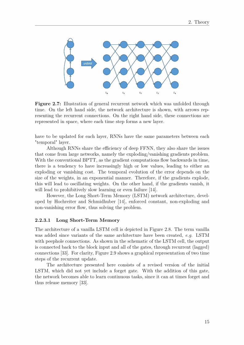
Figure 2.7: Illustration of general recurrent network which was unfolded throughtime. On the left hand side, the network architecture is shown, with arrows rep-resenting the recurrent connections. On the right hand side, these connections arerepresented in space, where each time step forms a new layer.

have to be updated for each layer, RNNs have the same parameters between each"temporal" layer.

Although RNNs share the efficiency of deep FFNN, they also share the issuesthat come from large networks, namely the exploding/vanishing gradients problem.With the conventional BPTT, as the gradient computations flow backwards in time,there is a tendency to have increasingly high or low values, leading to either anexploding or vanishing cost. The temporal evolution of the error depends on thesize of the weights, in an exponential manner. Therefore, if the gradients explode,this will lead to oscillating weights. On the other hand, if the gradients vanish, itwill lead to prohibitively slow learning or even failure [14].

However, the Long Short-Term Memory (LSTM) network architecture, devel-oped by Hochreiter and Schmidhuber [14], enforced constant, non-exploding andnon-vanishing error flow, thus solving the problem.

2.2.3.1 Long Short-Term Memory

The architecture of a vanilla LSTM cell is depicted in Figure 2.8. The term vanillawas added since variants of the same architecture have been created, e.g. LSTMwith peephole connections. As shown in the schematic of the LSTM cell, the outputis connected back to the block input and all of the gates, through recurrent (lagged)connections [33]. For clarity, Figure 2.9 shows a graphical representation of two timesteps of the recurrent update.

The architecture presented here consists of a revised version of the initialLSTM, which did not yet include a forget gate. With the addition of this gate,the network becomes able to learn continuous tasks, since it can at times forget andthus release memory [33].

15

2. Theory

Figure 2.8: Schematic of vanilla LSTM architecture. The recurrent connectionsare noted by arrows with time-lags. The gate activation functions, noted by g,are always sigmoids, while the input g and output h usually have tanh activationfunctions.

The formulas for the forward pass in a vanilla LSTM are given in equations(2.20) through (2.25). For clarity, the notation is vectorised and follows the orderin Figure 2.8.

zcurrent = g(Wzx

current +Rzyprevious + θz

)input (2.20)

icurrent = g(Wix

current +Riyprevious + θi

)input gate (2.21)

f current = g(Wfx

current +Rfyprevious + θf

)forget gate (2.22)

ccurrent = icurrent � zcurrent + f current � cprevious cell state (2.23)ocurrent = g

(Wox

current +Royprevious + θo

)output gate (2.24)

ycurrent = ocurrent � h(ccurrent

)output (2.25)

Here � denotes point-wise multiplication of two vectors. W and R are the weightsmatrices. They are noted differently since W consists of the input weights rectan-gular matrices and R are square recurrent weight matrices.

2.3 LearningAs previously mentioned, backpropagation is the fundamental principle which al-lows deep networks to learn. However, it is merely a computation step taken by acertain optimisation algorithm, such as gradient descent. It is the optimiser that de-termines how the network updates the weights towards the minimisation of the lossfunction. In section 2.3.1 there will be a short description of the relevant loss func-tions, followed by the optimisation algorithm used in this thesis (section 2.3.2), andfinally some of the regularisation strategies to improve the network’s generalisationcapabilities, in section 2.3.3.

16

2. Theory

Figure 2.9: Schematic of two time steps of the LSTM update. The notation t− 1represents the previous time step and t the current time step. With a single LSTMcell, there is a sequence of inputs, x and outputs y, while typically only the lastoutput is considered for classification applications.

The goal of the ANN training process is to learn how to map the input datato the output data, so that a high classification accuracy is reached. This is alsoreferred to as achieving a low bias network. Conversely, if a network fails to learnand produces low accuracies, it has a high bias. However, for a classifier to beuseful, besides having a low bias, it needs to perform equally well on unseen dataas on the training data, and therefore have low variance. Since the training datausually consists of a small sample from a certain pool of data, ANNs can learnthe entire sample with an accuracy of 100%, and then perform poorly with othersamples from the same pool. When this occurs, the network is said to have highvariance [34].

Further, when a network is said to have high bias, it means that there wasunderfitting to the training data, and that it could not learn efficiently. On theother hand, when there is high classification accuracy and the test accuracy is signif-icantly lower, the network may suffer from high variance, meaning that overfittingoccurred [34,35].

2.3.1 Loss FunctionThere are several possible loss functions to be employed for training neural networks.The choice of loss depends on the problem at hand. For regression problems, wherethe network needs to learn a specific function, the appropriate loss would be similarto the one in equation (2.7), based on the distance between input and output (resid-ual). However, for classification problems, such as myoelectric pattern recognition,there are more efficient entropy-based loss functions.

Depending on the desired output format of the classification problem, it may bebetter to use binary or categorical cross-entropy, where the first is merely a specialcase of the second. In problems where there are only two output classes, binarycross-entropy is the obvious choice. However, if there is a multi-class problem wheremultiple outputs can be present for a given input, it becomes a multi-label situation.In such cases, binary cross-entropy can be used. However, in order to use a binary

17

2. Theory

loss with more than two output nodes, the output activation cannot be a softmaxfunction, but an alternative such as the sigmoid function. This will result in aclassifier made up of a group of binary classifiers.

The binary cross-entropy loss function is presented in equation (2.26), with yrepresenting the output of the network and y the target value ∈ 0, 1.

L (y, y) = − [ylog (y) + (1− y) log (1− y)] (2.26)where y can be seen as the probability of the output being 1, and (1− y) theprobability of the output being 0.

In order to employ such a loss function to a multi-class problem, it is necessaryto encode the outputs into binary arrays, with size equal to the number of classes,K. For example, in a problem with five possible outputs, the one-hot encoded vectorfor the second class would be: y2 = {0, 1, 0, 0, 0}. In equation (2.27), the categoricalcross-entropy loss is presented.

L (y, y) = −K∑k=1

yklog (yk) (2.27)

where yk is the kth output node and log indicates the natural logarithm, which iswhy this is also sometimes called the log loss. Note that the output represents aprobability distribution computed by the softmax layer.

Upon choosing the appropriate loss function, the optimisation goal can bewritten in the form of a loss function to be minimised with respect to the wholedataset:

J(w[1], θ[1], ..., w[L], θ[L]

)= 1p

p∑µ=1L(y(µ), y(µ)

)(2.28)

where Lmay represent any of the loss functions introduced, or even another speciallydesigned for a certain problem, as long as it is differentiable. Note that the costfunction is minimised with respect to all network parameters and averaged by all pexamples. This is called batch gradient descent because the whole batch of trainingexamples is used to compute the cost function.

2.3.2 Optimisation AlgorithmThough a gradient descent step will always lead to a decrease of the cost function,propagating the entire training set trough the network to obtain a single step iscomputationally expensive. Furthermore, if the gradient gets smaller, the algorithmbecomes increasingly slow. Finally, for deep neural networks it may even be unfea-sible to keep all that data in the main memory. Consequently, the most extensivelyused optimisation algorithm for training large networks is stochastic gradient descent(SGD).

Though the update rule for SGD is essentially the same, the network parame-ters get updated after each input-output example, similarly to the perceptron algo-rithm. Additionally, the inputs are ramdomly shuffled before every epoch. However,due to its stochastic nature, the cost is no longer guaranteed to decrease monoton-ically. Nonetheless, this may come as an advantage, since gradient descent will getstuck in local minima and the stochasticity provides a way to escape them.

18

2. Theory

Perhaps as a way to include the best of both algorithms, the mini-batch train-ing method was developed. By dividing the training set into smaller batches andusing these to update the network, better estimates of the gradient are obtained. Itis easy to understand that with a batch size of 1, the mini-batch algorithm is simplySGD, and with a batch size equal o the training set it becomes gradient descent.By using the mini-batch SGD algorithm, there are two parameters that need to bechosen for optimisation, namely the learning rate, η, and the batch size.

Recently, more efficient stochastic optimisation methods have been developed,such as RMSprop and AdaGrad. The optimisation algorithm implemented in thisthesis was the Adam algorithm, which was developed by Kingma and Ba [36] andhas shown to be a comparably better optimiser since it attempt to combine theadvantages of the other two algorithms. The name derives from Adaptive momentestimation, because the algorithm estimates the first and second moments of thegradients and then computes individual adaptive learning rates, for the update rule.This rule can be seen in equation (2.29).

wcurrent = wprevious − α mcurrent

√vcurrent + ε

(2.29)

Where m and v, are estimates of the first and raw second moments of the gradients,noted as g. The are computed in accordance with equations (2.30) and (2.31).

mcurrent = β1 ·mprevious + (1− β1) · gcurrent (2.30)vcurrent = β2 · vprevious + (1− β2) · (gcurrent)2 (2.31)

These equations consist of exponential moving averages of the gradient, m, and thesquared gradient, v. Where the first is an estimate of the 1st moment (the mean) andthe latter is the 2nd raw moment (the uncentred variance). The hyperparametersβ1 and β2 ∈ [0, 1) control the rates of exponential decay of each moving average.However, because these vectors are initialised to zero, they are biased towards zero.The algorithm them uses bias correction terms, shown in equations (2.32) and (2.33),to compute m and v.

mcurrent = mcurrent

(1− βc1) (2.32)

vcurrent = vcurrent

(1− βc2) (2.33)

where c is the current iteration number. This means that at each step, both βc

parameters get increasingly smaller and this initialisation bias correction has a pro-gressively lower impact on the update [36].

The authors included in their paper the set of advised default parameters:α = 0.001, β1 = 0.9, β2 = 0.999 and ε = 10−8 [36].

2.3.3 Regularisation MethodsThe goal of regularisation methods is to improve the generalisation ability of thenetwork, by reducing the difference between the training error ans the test error.This difference can be considered as the generalisation error, and there are severalstrategies to reduce it [34].

19

2. Theory

2.3.3.1 L2-Regularisation

The main regularisation method to be presented here is the L2-regularisation of thecost function. This works by adding an extra penalty term to the cost function,as can be seen in equation (2.34), where L is the loss function, e.g. categoricalcross-entropy.

J(w[1], θ[1], ..., w[L], θ[L]

)= 1p

p∑µ=1L(y(µ), y(µ))

)+ λ

2p

L∑l=1

∥∥∥w[l]∥∥∥2

(2.34)

Where the norm is computed as in equation (2.35). Corresponding to the Frobeniusnorm of a matrix, it is equal to the sum of squared elements of a matrix.

∥∥∥w[l]∥∥∥2

=n[l+1]∑i=1

n[l]∑j=1

(wij)2 (2.35)

The cost function is minimised with respect to all weights and biases of the networkwith L layers. Because of the penalty that will increase the cost if the weights are toolarge, this regularisation method will force the weights to be small. For this reason,it is sometimes referred to as weight decay. The regularisation parameter, λ, istherefore another hyperparameter to be tuned.

2.3.3.2 Dropout

In recent years, a new type of regularisation method has been introduced, namelythe dropout method. It has shown to reduce overfitting at a low computationalcost. By sequentially dropping out a set of nodes, it becomes possible to combineexponentially many smaller architectures within the same model. The choice ofwhich nodes to drop is random, and determined by a probability parameter [35].Though it seems to have become common practice to apply dropout on deep CNNmodels, it will not be implemented in this thesis.

2.3.3.3 Data Augmentation

One of the key requirements for deep learning applications is the availability of largequantities of data. Deep models, with more trainable parameters than number oftraining examples can still have relatively low generalisation error [34]. Nonetheless,when there is an insufficient amount of training data, the models tend to overfit tothat data, and end up having bad generalisation capability. Though the ideal is toget additional data, when that is not possible, alternative regularisation strategiescan be employed to expand from the available data. Such methods are referred toas data augmentation.

Though more sophisticated methods exist, a simple way of obtaining moretraining data is to modify the available data. In image classification problems this isdone by applying geometric transformations and adding noise to the available images[37]. In one-dimensional signals, adding white Gaussian noise can produce a similareffect, by generating significantly different signals. This is the strategy employed byAtzori et al. [12] when using the Ninapro database for a CNN implementation.

20

2. Theory

2.3.3.4 Early stopping

Finally, the simplest strategy to make sure that the network can generalise well isto split the dataset into three sets: training, validation and test set. The reasoningbehind this is to be able to use the largest portion of the data for training the model,but keep a smaller sample of it to track the network’s performance on unseen data,i.e on the validation set. During training, if the error of the training set keepsdecreasing, but the validation error stagnates or even rises, it means that overfittinghas begun to occur. Early stopping is simply to check when or if this occurs and tostop training then.

The goal of the test set, independent to the validation set, is to make surethe training was not biased towards the validation set. This is due to the hyper-parameters (e.g. number of layers and nodes) that can be fine-tuned based on thelearning curve of the validation set . This also includes the stopping point, meaningthe epoch at which the learning stopped, since it is based on the accuracy for thevalidation data. The test set provides a truly unseen group of examples that willgive an unbiased evaluation of the model’s performance.

2.4 Performance Measures

The most straight forward way of evaluating the performance of a machine learningalgorithm is to measure the classification accuracy, which is equal to the fraction ofcorrect classifications with respect to the total number of classifications. However,this measure can give rise to deceivingly high performance results. To illustrate this,consider a binary classification problem, where 80% of test examples are positive andthe rest negative. If the classification algorithm were to classify all test examples aspositive, the accuracy would be 80%, even though it effectively could not recognisethe negative examples. This situation arises from an unbalanced class distribution,but can be avoided by having equal number of examples for each class.

To continue with the example above, let us introduce a few important conceptsby looking at the confusion matrix in table 2.2.

Table 2.2: Confusion matrix of a binary classification problem.

ytarget

ypredicted Positive Negative

Positive TP FNNegative FP TN

For binary classification problems, the confusion matrix gives a clear summaryof the algorithm’s performance. The terms TP, TN, FP and FN refer to true pos-itives, true negatives, false positives and false negatives, respectively. From thesevalues many different accuracy measures can be extrapolated, such as precision (truepositive rate) and recall (true negative rate) [38].

21

2. Theory

Accuracy = TP + TN

TP + TN + FP + FN× 100 (2.36)

Precision = TP

TP + FN× 100 (2.37)

Recall = TN

TN + FP× 100 (2.38)

The measures from equations (2.37) and (2.38) can further be used for more complexmeasures such as the F1-score (harmonic mean of precision and recall).

F1-score = 2 · Precision ·RecallPrecision+Recall

(2.39)

However, the F1-score has some drawbacks, especially when dealing with un-balanced classes. A measure that is more robust to class imbalance is the Matthew’sCorrelation Coefficient (MCC) [38]. Equation (2.40) shows the formula for comput-ing the MCC, using values from the confusion matrix.

MCC = TP × TN − FP × FN√(TP + FP )(TP + FN)(TN + FP )(TN + FN)

(2.40)

The MCC will be 1 for a perfect classifier and 0 for a random classifier. Addi-tionally, an inverse classifier will have an MCC of -1, which gives another dimensionto the performance measure. This score can be applied for multi-class classificationproblems however, all classes must be present in the classification output, otherwisethe measure becomes undefined [38,39] .

22

3Methods

In this chapter, there will be a detailed description of the Ninapro data, followedby the processing steps and finally the experiments. The aim is to clearly stateall processing executed before implementing the pattern recognition algorithms inorder to recreate the input to the models. The DNN models to be tested are a CNN,an RNN and a combination of the two types of networks, referred to as CNN-RNN.More details about the architectures as well as the experimental setup are presentedin section 3.4.

3.1 Dataset

The EMG data used for this thesis was obtained from the Ninapro repository, whichhas the aim of being a benchmark database for the field of non-invasive adaptivehand prosthetics [18,40]. To date, the repository includes seven different databases,with distinct acquisition protocols and subjects, but following a general guideline.The most recent database, is the only to include both intact and amputee subjects,which is why it was chosen as the source of data to be used here [21]. Though it wouldhave been possible to collect new data in the lab, it has become common practiceto resort to publicly available databases, such as the Ninapro, for benchmarkingdeep learning algorithms [12]. If new recordings would have been made, that wouldalso require more time while also making the comparison with other methos moredifficult. The following sections will introduce how the chosen dataset was recordedand processed.

3.1.1 Signal Acquisition

For the 7th Ninapro database, myoelectric recordings were made using a Delsys®

Trigno™ IM Wireless System, with a total of 12 active double–differential wirelesselectrodes. Each of the Trigno™ sensors also includes an Inertial Measurement Unit(IMU), capable of recording tri-axial accelerometer, gyroscope and magnetometermeasurements. While the EMG signals were acquired at a 2000 Hz sampling rate,the IM data was sampled at a much lower rate of 128 Hz. To compensate for thisdiscrepancy, the IM data was later up-sampled to a frequency of 2 kHz, by linearinterpolation [21]. While additional measurements are available on the database,these fall out of the scope of this thesis.

23

3. Methods

3.1.2 Sensor Placement

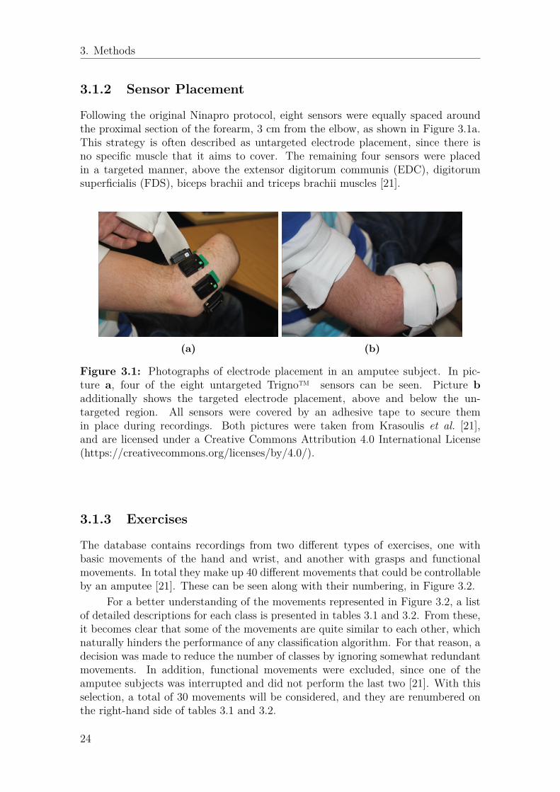
Following the original Ninapro protocol, eight sensors were equally spaced aroundthe proximal section of the forearm, 3 cm from the elbow, as shown in Figure 3.1a.This strategy is often described as untargeted electrode placement, since there isno specific muscle that it aims to cover. The remaining four sensors were placedin a targeted manner, above the extensor digitorum communis (EDC), digitorumsuperficialis (FDS), biceps brachii and triceps brachii muscles [21].

(a) (b)

Figure 3.1: Photographs of electrode placement in an amputee subject. In pic-ture a, four of the eight untargeted Trigno™ sensors can be seen. Picture badditionally shows the targeted electrode placement, above and below the un-targeted region. All sensors were covered by an adhesive tape to secure themin place during recordings. Both pictures were taken from Krasoulis et al. [21],and are licensed under a Creative Commons Attribution 4.0 International License(https://creativecommons.org/licenses/by/4.0/).

3.1.3 Exercises

The database contains recordings from two different types of exercises, one withbasic movements of the hand and wrist, and another with grasps and functionalmovements. In total they make up 40 different movements that could be controllableby an amputee [21]. These can be seen along with their numbering, in Figure 3.2.

For a better understanding of the movements represented in Figure 3.2, a listof detailed descriptions for each class is presented in tables 3.1 and 3.2. From these,it becomes clear that some of the movements are quite similar to each other, whichnaturally hinders the performance of any classification algorithm. For that reason, adecision was made to reduce the number of classes by ignoring somewhat redundantmovements. In addition, functional movements were excluded, since one of theamputee subjects was interrupted and did not perform the last two [21]. With thisselection, a total of 30 movements will be considered, and they are renumbered onthe right-hand side of tables 3.1 and 3.2.

24

3. Methods

(a)

(b)

Figure 3.2: Collection of movements executed by subjects in database 7 of theNinapro repository. Pictures in group a, correspond to movements from exercise1 and pictures in group b consists of the variety of functional grasps recorded forexercise 2. These photographs © [2015] IEEE were taken and rearranged fromAtzori et al. [18].

Table 3.1: Detailed description of movements from exercise 1. Sections in grayrepresent the original numbering found in Figure 3.2, with excluded movements.

1 Flexing all fingers except thumb (Thumb up) 12 Extension of index and middle finger while flexing oth-

ers (V-sign)2

3 Flexion of ring and little finger while extending others(German three)

3

4 Thumb opposing base of little finger (Four) 45 Abduction of the fingers (Open hand) 56 All fingers flexed (Close hand) 67 Extended index, with remaining fingers flexed (Index

pointer)7

Isometric,isotonic handpostures

8 Adduction of extended fingers (Joined fingers) 89 Wrist supination (rotation axis through middle finger) 910 Wrist pronation (rotation axis through middle finger) 1011 Wrist supination (rotation axis through little finger)12 Wrist pronation (rotation axis through little finger)13 Wrist flexion 1114 Wrist extension 1215 Wrist extension with closed hand 1316 Wrist radial deviation 14

Basicmovements ofthe wrist

17 Wrist ulnar deviation 15

25

3. Methods

Table 3.2: Detailed description of movements from exercise 2. Sections in grayrepresent the original numbering found in Figure 3.2, with excluded movements.

18 Large diameter grasp (1L bottle) 1619 Small diameter grasp (tube)20 Fixed hook grasp (glass) 1721 Index finger extension grasp (knife) 1822 Medium grasp (0.5L bottle vertical) 1923 Ring grasp (0.5L bottle horizontal) 2024 Prismatic four fingers grasp (pencil)25 Stick grasp (pencil) 2126 Writing tripod grasp (pen) 2227 Power grasp (sphere)28 Three finger grasp (sphere)29 Precision grasp (sphere)30 Tripod grasp (sphere) 2331 Prismatic grasp (coin) 2432 Tip pinch grasp (pill) 2533 Quadpod grasp (bottle cap) 2634 Lateral grasp (card) 2735 Parallel extension grasp (book) 2836 Extension type grasp (plate) 29

Grasps, withevery-dayobjects

37 Power grasp (disk) 3038 Open a bottle with tripod grasp39 Turn a screw (grasp the screwdriver with a stick grasp)Functional

movements 40 Cut something (grasp the knife with an index finger exten-sion grasp)

26

3. Methods

3.1.4 Data CollectionData was collected from a total of 20 intact and two amputee subjects, with ex-actly the same procedure. However, while the first group preformed each movementmonolaterally, the second was instructed to perform bilateral mirrored movements,to obtain a ground truth. This is a common practice which helps amputee subjectsto visualise the phantom limb moving in synchrony with their intact hand [18]. Eachsession required the subject to perform each movement six times, with 3 seconds restfollowed by 5 seconds contraction. This was done by providing a visual stimulus ona computer screen indicating which movement to perform [21]. Due to time limi-tations, it was decided to use only the first 8 intact subjects for the experiments,which gives a total of 10 test subjects.

3.1.5 Signal ProcessingIn addition to linearly interpolating the IM data, further processing stages wereapplied. First, to reduce power line interference, a Hampel filter was used on theEMG signals. Subsequently, a relabelling procedure was performed to align thevisual stimulus and the respective contraction [21]. This is a vital step for classifica-tion purposes, since the presence of mislabelled examples in training data can leadto poor results. Because there is an inevitable misalignment between the stimuliand the contraction periods, due to variable reaction time and attention span ofsubjects, the relabelling was done in accordance with the Ninapro protocol. For adescription of the procedure, refer to section III B of the paper by Atzori et al. [18].

3.2 Data ProcessingIn order to apply the desired machine learning algorithms to the Ninapro dataset,it was necessary to structure the data appropriately. The dataset was provided ina separate Matlab file for each subject and exercise, where all measured movementswere stacked into long vectors of non-contiguous signals. To produce the commaseparated value (CSV) file containing pairs of input and output vectors, some dataprocessing was performed.

The first step was to remove the redundant movements as mentioned in Section3.1.3, as well as measurements other than EMG and accelerometer values. Then dataaugmentation by a factor of 8 was performed as introduced in Section 2.3.3.3. Thiswas done by iteratively taking the original signals and adding white Gaussian noisewith increasing SNR from 10 to 40, with an increment of 5. The augmentationmagnitude was chosen by verifying the amount of data generated from the process.With a factor of 8 the size of the files reached approximately 4 GB per subject andexercise. If the networks were to be trained for both exercises simultaneously, thisvalue would therefore reach a total of 8 GB, which proved difficult to handle bythe hardware. Though there are methods to overcome these limitations, none wereexplored in this thesis, thus each exercise was evaluated independently. Furthermore,to add a reasonable amount of noise, two separate SNR values were used based onthe average signal power of the EMG and the accelerometer signals. To achieve

27

3. Methods

this, the inbuilt Matlab function awgn was used and seven new complete recordingsobtained. This process resulted in a total of 48 repetitions for each movement.

Subsequently, the accelerometer signals were down-sampled to 500 Hz, in anattempt to reduce the amount of computation time needed. Based of the work byAtzori et al. [12], the EMG data was RMS rectified to the same frequency as theaccelerometer data, so that more information was preserved in the final signal whilealso attenuating the effects of outliers.

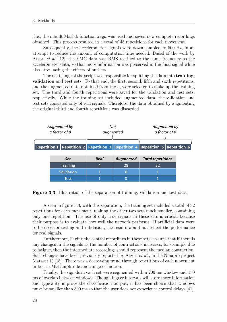
The next stage of the script was responsible for splitting the data into training,validation and test sets. To that end, the first, second, fifth and sixth repetitions,and the augmented data obtained from these, were selected to make up the trainingset. The third and fourth repetitions were saved for the validation and test sets,respectively. While the training set included augmented data, the validation andtest sets consisted only of real signals. Therefore, the data obtained by augmentingthe original third and fourth repetitions was discarded.

Figure 3.3: Illustration of the separation of training, validation and test data.

A seen in figure 3.3, with this separation, the training set included a total of 32repetitions for each movement, making the other two sets much smaller, containingonly one repetition. The use of only true signals in these sets is crucial becausetheir purpose is to evaluate how well the network performs. If artificial data wereto be used for testing and validation, the results would not reflect the performancefor real signals.

Furthermore, having the central recordings in these sets, assures that if there isany changes in the signals as the number of contractions increases, for example dueto fatigue, then the intermediate recordings should represent the median contraction.Such changes have been previously reported by Atzori et al., in the Ninapro project(dataset 1) [18]. There was a decreasing trend through repetitions of each movementin both EMG amplitude and range of motion.

Finally, the signals in each set were segmented with a 200 ms window and 150ms of overlap between windows. Though bigger intervals will store more informationand typicality improve the classification output, it has been shown that windowsmust be smaller than 300 ms so that the user does not experience control delays [41].

28

3. Methods

Once all the data was processed, it was stored in a separate CSV file for eachset. Groups of three sets were stored in separate folders according to exercise andsubject to be accessible for testing.

3.3 Software and HardwareOnce the data was structured and stored appropriately, it could be imported to thePython program developed to run the different deep learning algorithms. This wasimplemented in a virtual environment created using Anaconda. In this environmentMicrosoft’s Cognitive Toolkit (CNTK) was installed along with other necessary li-braries. CNTK is an open source deep learning framework that can be importedhas a library to Python, C++ or C# programs, as well as a standalone tool inthe model description language, BrainScript [42]. Python was chosen due to itssimplicity as well as the compatibility with a well established library supported byother major deep learning frameworks, such as Theano and TensorFlow. The Keraslibrary provides a simple high level method of programming neural networks, withan intuitive and well documented API. Therefore, Keras is an ideal choice for a highlevel implementation of complex networks, such as CNNs and LSTMs [43].

For deep learning applications, there has to be a careful choice of hardwareas well as software, since they require computational power superior to most com-mercially available computers. The system used for the following experiments was a64-bit Windows based computer, with a CUDA-enabled GPU by NVIDIA, namelythe GeForce GTX 970 model, with 4 GB dedicated memory. Other relevant systemspecifications include a 16 GB RAM and an Intel® Core™ i7 CPU. In the resultsthere will be an evaluation of the execution time for the different networks whichhighly depends on the system used together with the selected software.

3.4 ExperimentsFor the experimental stage of this thesis, the CSV files were loaded into a Pythonscript and the input-target pairs stored in separate NumPy arrays. Here, as de-scribed in section 2.3.1, the target classes had to be transformed from integers intoone hot encoded vectors. The final step before training the networks was to balanceall the classes within the sets. This was essential because the class of no movementor rest, had three times more samples than the other movement classes. Thus, twothirds of the windows labelled as rest had to be discarded from each set. For thatpurpose, before each run, windows classified as rest were randomly removed fromall sets. In addition, the movement classes were also subjected to random deletionof a small number of windows so that all sets contained exactly the same numberof examples as the least represented movement. To improve training, the exampleswere also randomised, before each run.

To evaluate the DNN models, three different architectures were tested on tensubjects for both exercises. Once a comparison was made between these structures,the one that provided the best result was further optimised by searching the hyper-parameter space.

29

3. Methods

3.4.1 Model ComparisonThe three architectures to be compared are a CNN, RNN and CNN-RNN model.Because there are many hyperparameters that influence the performance of DNNs,in this phase of the experiment, a fix set of parameters were chosen and used for allthree structures. The only hyperparameter that was different between networks wasthe number of layers, since these behave differently for RNNs and CNNs. Schematicsof the architectures can be found in figures 3.4, 3.5 and 3.6, and the set of parametersused is presented in table 3.3.

Figure 3.4: Schematic of CNN model. The input is fed to a sequence of convolu-tional and max-pooling layers. The sizes of the layer outputs are annotated beloweach layer. At the end there is a softmax layer with 16 nodes, one for each class.Though not represented in the schematic, the outputs of the last max-pooling layerwere stacked into one large vector before being fed to the output layer.

The CNN structure was inspired by the VGGNet architecture, due to its sim-plicity and reported success in other applications. The network developed by theVisual Geometry Group at Oxford, has the key characteristic of containing only 3x3filters in the convolutional layers, and 2x2 in the max-pooling layers. However, theoriginal paper had a much deeper network with 16-19 weight layers. Of these, threewere fully-connected added at the end, just before the softmax layer. Finally, allconvolutional layers had ReLUs has activation functions [44].

The RNN model is perhaps the simplest, as it includes only one layer of LSTMunits and is followed by a softmax layer. When implementing recurrent networks,there is a possibility to predict several time steps from each input window, since thenodes have temporal depth (i.e. many-to-many configuration). However, for thepurpose of immediate movement classification this was not necessary, therefore amany-to-one configuration was used, meaning that each node outputs a single valueto the softmax layer.

There have been several attempts to create hybrid architectures with CNNsand RNNs. Perhaps the most relevant example is the recent work by Xia et al.which employed a CNN-RNN model for EMG based estimation of limb movements[45]. The strategy proposed in this thesis consists of a quite similar model withan initial CNN architecture, responsible for feature extraction and dimensionality

30

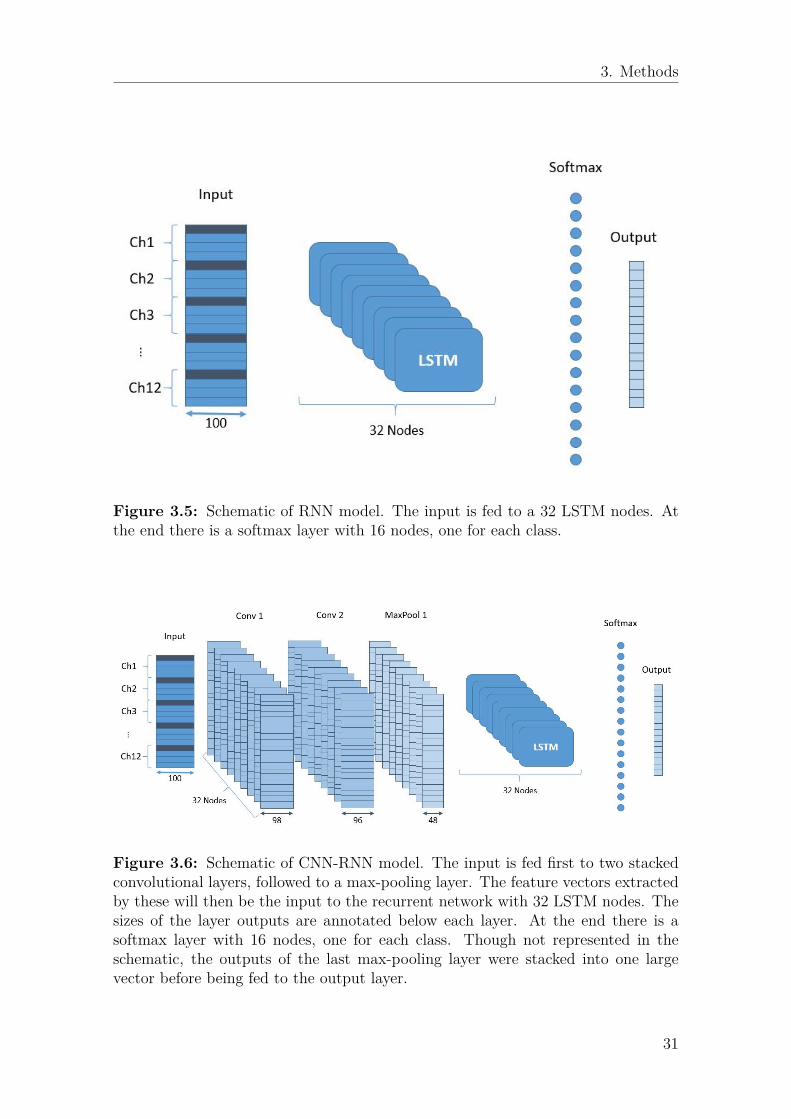
3. Methods

Figure 3.5: Schematic of RNN model. The input is fed to a 32 LSTM nodes. Atthe end there is a softmax layer with 16 nodes, one for each class.

Figure 3.6: Schematic of CNN-RNN model. The input is fed first to two stackedconvolutional layers, followed to a max-pooling layer. The feature vectors extractedby these will then be the input to the recurrent network with 32 LSTM nodes. Thesizes of the layer outputs are annotated below each layer. At the end there is asoftmax layer with 16 nodes, one for each class. Though not represented in theschematic, the outputs of the last max-pooling layer were stacked into one largevector before being fed to the output layer.

31

3. Methods

reduction, followed by a recurrent layer for learning time-dependent characteristicsof the signals. In accordance with the other two architectures, the CNN layers usedReLU units, while the LSTM nodes maintained the activation functions shown infigure 2.8.

Table 3.3: Hyperparameter values kept constant, for model comparison.

Nodes 32Batch size 128Learning rate, η 0.001Regularisation parameter, λ 0.001

The choice of initial parameters was, for the most part, arbitrary. The num-ber of nodes repeats for each convolutional, pooling and recurrent layers in eacharchitecture. Therefore, depending on the depth of the architectures, it results in adifferent number of trainable parameters (i.e. weights and biases). With 32 nodesper layer, the CNN contains the most trainable parameters with a total of 37040, fol-lowed by the CNN-RNN with 16592, and finally the RNN containing 10896 trainableparameters.

Starting with a relatively high batch size of 128, helps keep the training processshort and therefore speed up the model comparison experiment. On the other hand,the learning rate and other optimiser parameters do not affect the total trainingtime. The learning rate was set as the default value for the Adam optimisation al-gorithm. While this was later changed for the hyperparameter search, all remainingoptimisation parameters (β1, β2 and ε) were left as the default values. Finally, theinitial regularisation parameter was chosen by trial and error from a few test runs.

In order to evaluate the performance of each algorithm, during training of amodel, after each epoch if there was an improvement in validation accuracy, theweights and biases were stored. At the end of 100 epochs, the model to provide thebest validation accuracy was used for testing. This can be seen as a sort of earlystopping as described in section 2.3.3.4.

3.4.2 Hyperparameter SearchIn deep learning applications, even after a good architecture is found, there is stilla need to search for potentially better hyperparameters, that improve the perfor-mance of the algorithm. There are several possible strategies to achieve this, such asperforming a grid search where several combinations of parameters are tested andthe results compared.

For the purpose of this thesis, a sequential search was performed to see theeffects of each parameter on the learning curves. Each parameter was changedat a time, while keeping the others constant. The test model was updated for 100epochs and the resulting accuracies recorded. At the end of each test, the parametervalue that provided the best result was kept for the subsequent tests. Here, as forthe model comparison experiment, the accuracies were obtained using the test set.Therefore, by executing the parameter search using a constant set for testing, thehyperparameters chosen become biased towards this set. To guarantee that a set of

32

3. Methods

parameters outperforms another for unseen data, the test set should be chosen atrandom for each run, and the accuracy averaged over many runs.

Ideally there would also be a more comprehensive and rigorous hyperparam-eter search, with a heavily sampled search space, for more significant conclusions.However, since the goal of this experiment is mainly to explore the effects of eachhyperparameter on the learning process, only four new values were tested for eachparameter, in three separate trials. The values selected were picked at random froma constrained range.

Typically the learning rate takes values between 0.0001 and 1, for that reasona logarithmic scale was used for randomly selecting the test values. Nodes and batchsize, were limited by the memory capacity of the system. Following convention, bothparameters took only powers of two as vales. Finally, the regularisation parameterwas sampled in a similar range as the learning rate. Because it belongs to the penaltyterm, it could take any value equal or larger than zero. However, if λ would be toolarge, the penalty would overpower the cost function.

Due to the stochastic nature of the training, an individual run carries littleinformation on the efficacy of the chosen parameters. By running the same modelrepeatedly, the results can be averaged to reduce variability. Though three runs isstill not enough for statistically significant conclusions, it gives an intuition on howthe different parameters affect the learning process.

33

3. Methods

34

4Results

This chapter summarises the findings from the model comparison experiment as wellas the hyperparameter search. All results presented are discussed in an attempt toevaluate the potential of implementing these deep neural networks for myoelectricpattern recognition applications. Furthermore, the effects of each hyperparameterwere discussed to gain a better insight on their influence during training.

4.1 Model ComparisonIn order to compare the three architectures, each model was trained once for eachof the ten subjects, first for the movement classes from exercise 1, and then fromexercise 2. This resulted in 20 runs per algorithm, for a total of 60 trained models.Tables 4.1, 4.2 and 4.3 contain the results from this experiment. In addition toaccuracy and MCC score, three other measures were recorded: the time it tookto train the network, tTrain, the time it took to evaluate one window and get aclassification output, tTest/w, and the epoch at which the model was obtained (bestvalidation accuracy).

In terms of classification performance, the best network, with an average ac-curacy of 89.42% was the RNN model. Table 4.2 shows the cases in which the CNNmodel outperformed the RNN with the † symbol, and ‡ denotes the cases where theCNN-RNN model performed better. Naturally, since the models are of a stochasticnature, these five samples in which the RNN did not outperform both models mayhave been a result of an unfortunate run. To be certain, this experiment shouldhave included multiple trials to average over, however, there was a time constraint.

While the CNN model took on average, approximately 4 minutes to train,the RNN took around 31 minutes. One of the benefits of having the CNN-RNNhybrid model is that the initial CNN structure reduces the input dimensionality ofthe LSTM cells, thus speeding up the training to an average of 18 minutes.

When comparing test times of the different models, the CNN was the consider-ably faster at producing a classification output when given an input window, takingon average only 1.25 ms. The CNN-RNN model followed with 11.82 ms and finallythe RNN took 20.20 ms.

There is not a lot that can be concluded about the learning process from theepoch at which the best model was obtained. A better indication is to look at thelearning curves of the training and validation set to observe when overfitting startsto occur. However, if the best validation accuracy is obtained in an early epoch,it may indicate that the learning rate is to high. Similarly, if the best model is

35

4. Results

Table 4.1: CNN results for ten subjects, separated by exercise. The mean accuracywas 86.27% (E1:87.70%, E2:84.84%), while the average MCC was 0.8558 (E1:0.8709,E2:0.8406). Training times (tTrain) were between 3 and 5 minutes, and the averagetest time (tTest per input window w) was 1.25 ms. The early-stopping epoch is notedfor each subject and was based on the validation accuracy. The early-stopping epochis noted for each subject and was based on the validation accuracy. The † symboldenotes the results obtained with the CNN that outperformed the RNN for the samesubject and exercise.

(a) Exercise 1

Subject Accuracy (%) MCC tTrain (min) tTest/w (ms) Epoch

1 94.33 0.9399 3 1.1926 532 92.47 0.9201 3 1.2356 763 91.86 0.9160 3 1.2391 584 96.88 0.9668 4 1.1926 575 85.20 0.8451 3 1.2620 806 90.00 0.8965 4 1.2449 217 92.07 0.9159 3 1.2194 208 83.59 0.8298 4 1.3256 9221 80.83 0.7984 3 1.2267 2522 69.74 0.6803 3 1.2155 65

(b) Exercise 2

Subject Accuracy (%) MCC tTrain (min) tTest/w (ms) Epoch

1 90.45 0.8990 4 1.1822 892 88.02 0.8745 5 1.3150 333 93.86 0.9355 4 1.2481 934 86.22 0.8557 5 1.2246 905 85.51 0.8482 4 1.2296 746 93.96† 0.9361† 4 1.2046 957 87.66 0.8705 3 1.4025 918 90.00 0.8952 4 1.1976 10021 49.47 0.4675 4 1.1867 10022 83.24† 0.8237† 3 1.3828 81

obtained near the one hundredth epoch, it may be that the learning rate should beincreased or that the training should be extended to more epochs.

To summarise the model comparison, the classification results were compiledinto Figure 4.1, in the form of boxplots. From these, the same conclusion was taken,namely that the RNN outperformed the other two models. With a median accuracyof of 91.81% (MCC = 0.9135), compared with 89.01% (MCC = 0.8849) for the CNNand 90.43% (MCC = 0.8990) for the CNN-RNN, the RNN model was chosen for thehyperparameter search. Although, by selection of better parameters for the othermodels could potentially lead them to outperform the RNN.

36

4. Results

Table 4.2: RNN results for ten subjects, separated by exercise. The mean accuracywas 89.42% (E1:91.38%, E2:87.47%), while the average MCC was 0.8889 (E1:0.9088,E2:0.8690). Training times (tTrain) were between 24 and 46 minutes, and the averagetest time (tTest per input window w) was 20.20 ms. The early-stopping epoch isnoted for each subject and was based on the validation accuracy. The results forwhich the † and ‡ symbola are appended show instances in which the RNN wasoutperformed by the CNN and CNNR-RNN models, respectively.

(a) Exercise 1

Subject Accuracy (%) MCC tTrain (min) tTest/w (ms) Epoch

1 94.91 0.9460 26 21.0467 462 93.75 0.9338 29 20.2995 583 99.13 0.9907 24 20.0171 844 97.72 0.9758 30 20.3820 795 92.27 0.9182 22 20.1575 676 90.80‡ 0.9026‡ 31 19.8325 557 95.73 0.9548 25 22.3052 918 86.99 0.8645 31 20.3809 8321 89.17 0.8859 25 20.7791 4722 73.30 0.7160 25 19.5468 96

(b) Exercise 2

Subject Accuracy (%) MCC tTrain (min) tTest/w (ms) Epoch

1 91.25 0.9075 34 20.1043 932 91.35 0.9088 39 20.9211 543 94.31 0.9401 32 19.5972 924 86.86‡ 0.8630‡ 46 19.3947 815 93.47 0.9305 35 19.3309 866 93.33† 0.9300† 37 20.0148 847 90.71 0.9024 24 20.4519 488 92.31‡ 0.9192‡ 33 19.5547 10021 59.71 0.5732 37 20.0887 8322 81.39† 0.8149† 26 19.6957 65

As seen in Figure 4.1, there are outliers in the data. These correspond to theresults from subject 21 on exercise 2. For all networks, the classification performancefor this exercise was substantially lower than the other participants and even for thesame participant on exercise 1. This may indicate that the amputee subject hadmore difficulties performing the movements from this exercise, resulting in worserecordings. When looking at Figure 3.2b, with the movements from exercise 2, it isunderstandable why an amputee would have difficulties recreating these movements.

37

4. Results

Table 4.3: CNN-RNN results for ten subjects, separated by exercise. The meanaccuracy was 85.69% (E1:87.82%, E2:83.56%), while the average MCC was 0.8490(E1:0.8715, E2:0.8265). Training times (tTrain) were between 13 and 28 minutes,and the average test time (tTest per input window w) was 11.82 ms. The early-stopping epoch is noted for each subject and was based on the validation accuracy.The ‡ symbol denotes the results obtained with the CNN-RNN that outperformedthe RNN for the same subject and exercise.

(a) Exercise 1

Subject Accuracy (%) MCC tTrain (min) tTest/w (ms) Epoch

1 92.44 0.9204 15 11.6438 232 92.98 0.9257 17 11.7232 363 96.66 0.9645 14 12.0112 474 96.88 0.9668 18 11.6034 325 87.60 0.8691 13 11.6746 966 91.59‡ 0.9109‡ 18 11.9243 177 91.16 0.9065 15 11.6649 238 80.48 0.7974 18 12.2664 5421 82.36 0.8136 15 12.0728 1422 66.05 0.6401 15 11.6535 82

(b) Exercise 2

Subject Accuracy (%) MCC tTrain (min) tTest/w (ms) Epoch

1 90.80 0.9028 20 11.3705 422 90.83 0.9027 23 12.0714 333 92.52 0.9212 19 11.4918 394 87.82‡ 0.8726‡ 28 11.8096 285 79.26 0.7808 21 12.0017 846 87.08 0.8649 22 11.4452 527 90.06 0.8954 14 12.3661 618 92.79‡ 0.9249‡ 20 11.5054 9621 46.41 0.4316 23 12.4690 9622 77.98 0.7685 15 11.6596 96

Finally, it can be concluded from the interquartile range (IQR) values that theRNN also provided the lowest variability, as opposed to the CNN-RNN which hadthe highest IQR of approximately 10% in accuracy. Even though variability is tobe expected when dealing with different subjects along with stochastic models, it isclear that the CNN-RNN model was more variable than the other two.

38

4. Results

CNN RNN CNN-RNN40

50

60

70

80

90

100Accuracy (%)

(a)

CNN RNN CNN-RNN0.4

0.5

0.6

0.7

0.8

0.9

1.0

MCC

(b)

Figure 4.1: Tukey boxplots with classification results for each architecture. Thewhiskers have length equal to 1.5×IQR and were computed from the results in tables4.1, 4.2 and 4.3. These show the RNN outperforming the other two architectureswith a median value of 91.81%.

4.2 Hyperparameter SearchThe results from the hyperparameter search were compiled in Table 4.4. Since theexperiments were done sequentially, a total of five values were actually tested foreach parameter. Because the first hyperparameter to be tested was the learningrate, the initial model, with η = 0.001 had to be tested for two additional trials.This resulted in a reference average initial accuracy of 95.25% and MCC score of0.9495.

Table 4.4: Hyperparameter search results separated by parameter. The valuescorrespond to averages over three runs.

(a) Learning rate, η

η Accuracy (%) MCC

0.0001 94.81 0.94490.0006 95.93 0.95680.0040 92.54 0.92180.0253 77.91 0.7680

(b) Number of nodes

Nodes Accuracy (%) MCC

16 93.65 0.932864 94.72 0.9439128 93.07 0.9266256 92.93 0.9255

(c) Batch size

Batch Accuracy (%) MCC

16 93.65 0.933932 94.62 0.942964 94.57 0.9425256 93.56 0.9318

(d) Regularisation parameter, λ

λ Accuracy (%) MCC

0 95.49 0.95220.04 91.38 0.91010.2 88.66 0.88071 82.17 0.8117

39

4. Results

The best result is shown in bold, and was obtained with the initial number ofnodes and batch size, namely 32 nodes and batch size of 128. The effect of changinglearning rate can be seen in Figure 4.2a. It can be concluded that a learning ratebetween 0.0001 and 0.001 produces the best results. Because there were insufficienttrials, there is no certainty that η = 0.0006 is in fact the best value, however, fromthe small sample obtained, it produced the best result.

0.0001 0.001 0.01Learning rate, η

70

75

80

85

90

95

100

Acc

uracy

(%)

(a)

0 ... 0.01 0.1 1Regularisation parameter, λ

70

75

80

85

90

95

100

Accuracy

(%)

(b)

Figure 4.2: Visualisation results from Table 4.4. From these plots, the effect ofthe learning rate and the regularisation parameter are shown with respect to theaccuracy. The data point in green corresponds to the best average accuracy obtainedfrom the hyperparameter search. There is a clear decrease in learning ability as thesevalues become too large.

From tables 4.4b and 4.4c there are little changes in accuracy with the valuestested in this experiment. However, it would have been unfeasible to test muchhigher values, due to the memory limitation of the system. Though the numberof nodes did not have any significant effect on the classification accuracy, it canbe seen in Figure 4.3a, that with the increase of number of nodes there is a linearincrease of number of parameters that need to be trained, has would be expected.In a similar way, Figure 4.3b shows the linear relationship between the batch sizeand the training time. This was also to be expected since the bigger the mini-batchsize, the fewer times the network needs to be evaluated and updated.

The final hyperparameter to be tested was the regularisation parameter. FromFigure 4.2b it becomes evident that λ cannot be too large. However, there is nosignificant improvement from having λ = 0.01, when compared with having noregularisation at all. In order to gain a better understanding of the effects of this,as well as the other hyperparameters, it is valuable to look at the learning curvesshown in figures 4.4 through 4.7.

It becomes clear from Figure 4.4 that the learning rate affects the speed atwhich the network converges. With η = 0.0001, the network seems to still belearning when it reaches 100 epochs. By increasing the learning rate to 0.0006,

40

4. Results

16 32 64 128 256Number of nodes

4432

10896

29968

92688

316432

Number of parameters

(a)

16 32 64 128 256Batch size

90

50

27

15

9

Training tim

e per epoch

(s)

(b)

Figure 4.3: Additional effects of hyperparameters. Figure 4.3a shows effect ofnumber of nodes on the total number of trainable parameters. Figure 4.3b showsthe effect of increasing batch size on the training time. These results were to beexpected since they are directly linked with the computational complexity of theprogram.

there is already significant improvement and the network rapidly converges to agood accuracy, until it starts overfitting. This turning point is very clear in Figure4.4b where the training curve intersects the validation curve. With η = 0.004 thenetwork still converges, however, it seems that initially the rate is too large resultingin large oscillations. Nevertheless, there seems to be no evidence of overfitting. whichmeans that values of this order of magnitude may produce better results. The samecannot be said for η = 0.0253, which clearly made the network incapable to learn.

The effect of the number of nodes, seen in Figure 4.5, is not as drastic. Itseems that with 16 nodes, the RNN learns slower, since at the end of 100 epochsit still did not converge. On the other hand, with 256 nodes, the network hadsignificantly higher variance at the end of the training. However, since early-stoppingwas implemented, this did not affect the accuracy measured for the test set.

The batch size also affected the speed of convergence of the network. FromFigure 4.6 there is a tendency for the network to converge increasingly slower asthe mini-batch size increases. This can be explained by the fact that with a smallerbatch, at the end of each epoch the model was updated more times than with alarger batch.

Finally, as had been concluded from 4.2b, the regularisation parameter canhave large effects on the learning process. With larger values of λ, the learningcurves become more linear. Perhaps by increasing the number of epochs these valueswould actually lead to good results. Nevertheless, the learning speed becomes tooslow for the 100 epoch tests. Moreover, the increase in overlap between the trainingcurve and the validation curve shows that the regularisation is efficient in keeping alow variance.

41

4. Results

0 20 40 60 80 100Epoch #

0

20

40

60

80

100

Accu

racy (%

)

training setvalidation set

(a) η = 0.0001

0 20 40 60 80 100Epoch #

0

20

40

60

80

100

Accu

racy (%

)

training setvalidation set

(b) η = 0.0006

0 20 40 60 80 100Epoch #

0

20

40

60

80

100

Accu

racy (%

)

training setvalidation set

(c) η = 0.004

0 20 40 60 80 100Epoch #

0

20

40

60

80

100

Accu

racy (%

)

training setvalidation set

(d) η = 0.0253

Figure 4.4: Learning curves for different learning rates shown in Table 4.4a. Eachplot corresponds to one of the three trials for a given parameter set. With a largerlearning rate, the network suffers from high bias.

42

4. Results

0 20 40 60 80 100Epoch #

0

20

40

60

80

100

Accu

racy (%

)

training setvalidation set

(a) nodes = 16

0 20 40 60 80 100Epoch #

0

20

40

60

80

100

Accu

racy (%

)

training setvalidation set

(b) nodes = 64

0 20 40 60 80 100Epoch #

0

20

40

60

80

100

Accu

racy (%

)

training setvalidation set

(c) nodes = 128

0 20 40 60 80 100Epoch #

0

20

40

60

80

100

Accu

racy (%

)

training setvalidation set

(d) nodes = 256

Figure 4.5: Learning curves for different number of nodes, shown in Table 4.4b.Each plot corresponds to one of the three trials for a given parameter set. Withmore number of nodes the validation accuracy drops below the training accuracy,which is a sign of high variance.

43

4. Results

0 20 40 60 80 100Epoch #

0

20

40

60

80

100

Accu

racy (%

)

training setvalidation set

(a) batch size = 16

0 20 40 60 80 100Epoch #

0

20

40

60

80

100

Accu

racy (%

)

training setvalidation set

(b) batch size = 32

0 20 40 60 80 100Epoch #

0

20

40

60

80

100

Accu

racy (%

)

training setvalidation set

(c) batch size = 64

0 20 40 60 80 100Epoch #

0

20

40

60

80

100

Accu

racy (%

)

training setvalidation set

(d) batch size = 256

Figure 4.6: Learning curves for different mini-batch sizes shown in Table 4.4c.Each plot corresponds to one of the three trials for a given parameter set. Thelearning curves for different batch sizes are not significantly different. In general, itseems that a smaller batch size leads to a faster convergence.

44

4. Results

0 20 40 60 80 100Epoch #

0

20

40

60

80

100

Accu

racy (%

)

training setvalidation set

(a) λ = 0

0 20 40 60 80 100Epoch #

0

20

40

60

80

100

Accu

racy (%

)

training setvalidation set

(b) λ = 0.04

0 20 40 60 80 100Epoch #

0

20

40

60

80

100

Accu

racy (%

)

training setvalidation set

(c) λ = 0.2

0 20 40 60 80 100Epoch #

0

20

40

60

80

100

Accu

racy (%

)

training setvalidation set

(d) λ = 1

Figure 4.7: Learning curves for different levels of regularisation, shown in Table4.4d. Each plot corresponds to one of the three trials for a given parameter set. Notethat plot 4.7a displays the learning curve without regularisation. From λ = 0.2, theregularisation effect overpowers the learning and leads to high bias.

45

4. Results

0 1 2 3 4 5 6 7 8 9 10 11 12 13 14 15Predicted movement (%)

0123456789

101112131415

Target m

ovem

ent (%)

79 0 0 0 0 10 0 7 0 0 0 0 0 0 0 00 92 0 0 4 0 0 0 0 0 0 0 0 0 0 04 0 84 0 4 0 3 0 1 0 0 0 0 0 0 00 0 1 90 4 0 0 0 0 0 0 2 0 0 0 00 4 3 0 83 0 3 2 0 0 0 0 0 0 0 02 0 0 0 0 88 0 0 1 0 0 0 0 2 0 04 0 2 0 0 2 85 0 0 0 0 0 0 0 1 28 0 0 0 0 0 0 85 2 1 0 1 0 0 0 01 0 0 1 0 3 0 2 74 1 0 8 5 0 0 02 0 0 0 0 0 0 0 2 89 2 0 0 0 0 01 0 0 0 0 0 0 1 0 3 87 3 1 0 0 00 0 0 0 0 0 0 0 2 2 2 86 4 0 0 04 0 0 0 0 0 0 2 0 0 0 0 90 0 0 00 0 0 0 0 0 0 0 0 0 0 0 0 95 2 13 1 0 0 0 0 0 0 0 0 0 0 5 1 87 01 1 0 0 0 0 0 0 1 0 0 0 0 3 0 89

(a) Exercise 1

0 16 17 18 19 20 21 22 23 24 25 26 27 28 29 30Predicted movement (%)

0161718192021222324252627282930

Target m

ovem

ent (%)

98 0 0 0 0 0 0 0 0 0 0 0 0 0 0 02 92 0 0 1 0 2 0 0 0 0 0 0 0 0 01 0 93 2 0 0 1 0 0 0 0 0 0 0 0 02 0 0 85 9 1 0 0 0 0 0 0 0 0 0 01 0 0 6 81 8 0 0 0 0 0 0 1 0 0 00 3 0 0 10 80 0 0 1 2 0 0 0 0 0 00 0 0 0 0 0 97 2 0 0 0 0 0 0 0 01 0 0 1 0 1 0 89 3 0 1 0 1 0 0 01 0 0 0 3 0 0 1 93 0 0 0 0 0 0 01 0 0 0 1 0 0 1 0 93 2 0 0 0 0 01 0 0 0 0 0 0 0 0 0 94 0 0 0 0 01 0 0 0 0 0 0 0 0 0 0 92 4 0 0 01 1 0 0 0 1 0 0 0 0 0 0 83 7 1 14 0 0 0 0 0 0 0 0 0 0 0 0 95 0 02 0 0 0 0 0 0 0 0 0 0 1 0 0 89 63 0 0 0 0 0 0 0 0 0 1 0 0 0 7 86

(b) Exercise 2

Figure 4.8: Confusion matrices for both exercises, averaged over all subjects, withthe final set of hyperparameters. The percentages were truncated to the nearestinteger for better visualisation. Despite leading to inconsistencies in the percentages,values smaller than 1% can be disregarded for the purpose of this analysis.

As a final evaluation of the results, the RNN model was once again trainedusing the best set of parameters with the data from all subjects and both exercises.The results were compiled in two separate confusion matrices shown in Figure 4.8.The percentages obtained were computed by averaging the results of the ten subjects,for each exercise.

By looking at Figure 4.8, a few observations can be extracted. For instance,the majority of the output classes were at some point misclassified as the rest class(i.e. no movement). This may be due to failure of the relabelling procedure, wherea time window during rest was labelled as a certain movement. Furthermore, theclass with the lowest accuracy consisted of class number 8 of exercise 1, with 74%.This movement consists of the adduction of extended fingers, which is actuated bythe palmar interossei muscles, which are located in the hand. Since the electrodeswere all placed in the proximal part of the forearm, these were most likely unableto detect the movement effectively.

46

5Discussion

This chapter will attempt to build from the discussion initiated in the results sectionand further discuss the significance of the findings of this thesis.

While the model comparison experiment was done by grouping together bothintact and amputee subjects, it is relevant to evaluate the results separately. Themean CNN accuracy was 90.13% for intact subjects and 70.82% for amputees. Thesame trend is observed for the RNN, with 92.81% and 75.89% for intact and am-putee subjects, respectively. The difference was even more noticeable for the hybridnetwork with 90.06% for intact and 68.20% for amputee subjects. Since the end-users of myoelectric control systems are for the most part amputees, these resultsreinforce the RNN as the best performing model.

For myoelectric control, the testing time is a limiting factor. In order to im-plement these networks in real time applications, for online classification, the timeit takes to compute an output needs to be sufficiently small. This requirement willdepend on the application and the hardware on witch it is implemented. Sincethe tests were run in an a high performing computer, there will likely be an in-crease in testing time for other systems. While software applications, such as forphantom-limb pain treatment, may be used via similar systems, prosthetic deviceshave embedded systems which are significantly more limited. Nonetheless, there isan effort from the research community to increase computing speeds of DNNs which,in the future will allow for larger models to be implemented on weaker devices [46].

Taking test time into consideration, the CNN model would be the most likelycandidate to be implemented in embedded devices, with the mean test time of 1.25ms. As previously stated, it is possible that by searching the hyperparameter spacefor the CNN network, this would reach or even surpass the performance of the RNN.

Although Atzori et al. [12] employed CNNs for classification of the Ninapromovements, they did not exclude redundant movements nor separate the two exer-cises into different classifiers. Furthermore, they also did not include accelerometerdata, therefore it is not possible to do a direct comparison of the accuracies achievedhere. On the other hand, the 7th Ninapro database was provided by Krasoulis etal. [21], where for the 40 movements and using an LDA classifier a median accuracyof 82.7% for intact subjects and 77.8% was achieved. This however, was includingall of the IMU data, namely three-axial accelerometer, gyroscope and magnetome-ter signals. From this work it was concluded that by employing all the IMU data,significantly improved classification accuracy.

47

5. Discussion

Initially it was attempted to use all the movements at once to train the clas-sifiers, but several issues were encountered. The first being the memory capacityof the system, which did not allow for data augmentation in such a case. In ad-dition, the classifiers proved to have difficulties distinguishing between movementsthat were too similar (e.g. movements 9-12 in Figure 3.2a), leading to poor ac-curacies. Finally, there was a certain reasoning behind splitting the two exercisesinto separate classifiers. Due to the significant differences of the exercises, it seemedlogical to have two modes between which the user could switch, depending if theywanted to control hand postures or grasps.

While the CNN implementation by Atzori et al. [12] was implemented usingtwo-dimensional filters, this was not the approach used for this thesis. The motiva-tion for this modification was based on the characteristics of the input signals. Bystacking the EMG signals into a matrix and applying e.g. 3x3 filters, the signalsfrom different channels are mixed together through the convolution operation, andvaluable information may be lost. Furthermore, CNNs are not rotation or inversioninvariant which attributes significant importance to the order in which the differentchannels are stacked. As mentioned in the theory, the CNNs learn local, transla-tion invariant features. This only makes sense if the signals are kept separate andone-dimensional convolution is used.

Due to the considerable variability between different myoelectric pattern recog-nition research, it is difficult to compare results. Overall the conclusion that canbe derived from the current work is that these networks are yet another type of PRalgorithm that can be employed to solve the problem.

Moving on to the hyperparameter search experiment, the results showed thatnumber of nodes and the batch size had little effect on the test accuracy of the RNN.On the other hand, the optimisation parameters can have a significant impact onthe learning curves, therefore they should be prioritised when tuning parameters.

48

6Conclusion

To conclude, there will be a short summary of results an discussion followed by somecomments on the work presented in this thesis as well as possible future work thatmay be relevant for the field of myoelectric pattern recognition.

With median accuracies above 80% achieved by all three models studied, itcan be concluded that these DNNs are powerful pattern recognition tools for myo-electric control applications. However, there have been higher accuracies reportedin offline studies with other PR algorithms. Although, contrary to such studies,the classification was done independently of any feature extraction phase and stillreached high performances.

The highest performing architecture, with a median accuracy of 91.81%, wasthe RNN consisting of a layer of LSTM units. This could support the hypothesisthat recurrent networks have an advantage when processing temporal data, such asEMG and IMU signals. This can also be supported by the higher median accuracyobtained by the hybrid CNN-RNN model, 90.4% when compared with the CNN,89.01%. Though, due to the higher variability of the CNN-RNN model, it achievedthe lowest average accuracy. Nevertheless, the median performance values indicatethat the networks containing LSTM units have an advantage.

Another factor that should be taken in to consideration, is that even thoughthe CNN performed worse, it is an order of magnitude faster at computing an outputthan the CNN-RNN and RNN models. By passing the input windows through theCNN layers to the LSTM layer, the hybrid architecture became twice as fast as theRNN. This is due to the automatic feature extraction and reduction by convolutionaland max-pooling layers, respectively.

The utility of DNNs for myoelectric control applications has not yet beenproven. These models are more complex to implement than other well establishedalgorithms such as LDA, and have high computational cost. For simple embeddedsystems, such as in prosthetic devices, they may not be a viable option until fasteralgorithms or systems are developed. However, DNNs have been gaining momentumin the research community, and have been tested in a growing number of fields. Thehigh pace in development of both deep learning software and processing power ofhardware may lead to more reliable myoelectric control.

49

6. Conclusion

50

References

[1] Aidan D Roche, Hubertus Rehbaum, Dario Farina, and Oskar C Aszmann.Prosthetic myoelectric control strategies: a clinical perspective. CurrentSurgery Reports, 2(3):44, 2014.

[2] Sophie M Wurth and Levi J Hargrove. A real-time comparison between di-rect control, sequential pattern recognition control and simultaneous patternrecognition control using a fitts’ law style assessment procedure. Journal ofneuroengineering and rehabilitation, 11(1):91, 2014.

[3] Susannah M Engdahl, Breanne P Christie, Brian Kelly, Alicia Davis, Cynthia AChestek, and Deanna H Gates. Surveying the interest of individuals with upperlimb loss in novel prosthetic control techniques. Journal of neuroengineeringand rehabilitation, 12(1):53, 2015.

[4] Angkoon Phinyomark, Pornchai Phukpattaranont, and Chusak Limsakul. Fea-ture reduction and selection for emg signal classification. Expert Systems withApplications, 39(8):7420–7431, 2012.

[5] Kevin Englehart, B Hudgin, and Philip A Parker. A wavelet-based continuousclassification scheme for multifunction myoelectric control. IEEE Transactionson Biomedical Engineering, 48(3):302–311, 2001.

[6] Max Ortiz-Catalan. Cardinality as a highly descriptive feature in myoelectricpattern recognition for decoding motor volition. Frontiers in neuroscience, 9,2015.

[7] Angkoon Phinyomark, Franck Quaine, Sylvie Charbonnier, Christine Serviere,Franck Tarpin-Bernard, and Yann Laurillau. Emg feature evaluation for im-proving myoelectric pattern recognition robustness. Expert Systems with Ap-plications, 40(12):4832–4840, 2013.

[8] Paul Kaufmann, Kevin Englehart, and Marco Platzner. Fluctuating emg sig-nals: Investigating long-term effects of pattern matching algorithms. In Engi-neering in Medicine and Biology Society (EMBC), 2010 Annual InternationalConference of the IEEE, pages 6357–6360. IEEE, 2010.

[9] Erik Scheme and Kevin Englehart. Training strategies for mitigating the effectof proportional control on classification in pattern recognition based myoelectriccontrol. Journal of prosthetics and orthotics: JPO, 25(2):76, 2013.

[10] Max Ortiz-Catalan, Bo Håkansson, and Rickard Brånemark. Real-time andsimultaneous control of artificial limbs based on pattern recognition algo-rithms. IEEE Transactions on Neural Systems and Rehabilitation Engineering,22(4):756–764, 2014.

[11] Afarin Nazemi and Ali Maleki. Artificial neural network classifier in comparisonwith lda and ls-svm classifiers to recognize 52 hand postures and movements. In

51

References

Computer and Knowledge Engineering (ICCKE), 2014 4th International eCon-ference on, pages 18–22. IEEE, 2014.

[12] Manfredo Atzori, Matteo Cognolato, and Henning Müller. Deep learning withconvolutional neural networks applied to electromyography data: A resource forthe classification of movements for prosthetic hands. Frontiers in neurorobotics,10, 2016.

[13] Michael Hüsken and Peter Stagge. Recurrent neural networks for time seriesclassification. Neurocomputing, 50:223–235, 2003.

[14] Sepp Hochreiter and Jürgen Schmidhuber. Long short-term memory. Neuralcomputation, 9(8):1735–1780, 1997.

[15] Kyunghyun Cho, Bart Van Merriënboer, Dzmitry Bahdanau, and Yoshua Ben-gio. On the properties of neural machine translation: Encoder-decoder ap-proaches. arXiv preprint arXiv:1409.1259, 2014.

[16] Wenpeng Yin, Katharina Kann, Mo Yu, and Hinrich Schütze. Compara-tive study of cnn and rnn for natural language processing. arXiv preprintarXiv:1702.01923, 2017.

[17] Yann LeCun, Yoshua Bengio, and Geoffrey Hinton. Deep learning. Nature,521(7553):436–444, 2015.

[18] Manfredo Atzori, Arjan Gijsberts, Ilja Kuzborskij, Simone Elsig, Anne-Gabrielle Mittaz Hager, Olivier Deriaz, Claudio Castellini, Henning Müller,and Barbara Caputo. Characterization of a benchmark database for myoelec-tric movement classification. IEEE Transactions on Neural Systems and Reha-bilitation Engineering, 23(1):73–83, 2015.

[19] John Webster. Medical instrumentation: application and design, chapter 4,pages 144–146,242. John Wiley & Sons, 4th edition, 2015.

[20] Melvin M Morrison. Inertial measurement unit, December 8 1987. US Patent4,711,125 A.

[21] Agamemnon Krasoulis, Iris Kyranou, Mustapha Suphi Erden, Kianoush Nazar-pour, and Sethu Vijayakumar. Improved prosthetic hand control with concur-rent use of myoelectric and inertial measurements. Journal of neuroengineeringand rehabilitation, 14(1):71, 2017.

[22] Warren S McCulloch and Walter Pitts. A logical calculus of the ideas immanentin nervous activity. The bulletin of mathematical biophysics, 5(4):115–133, 1943.

[23] Ivan Nunes Da Silva, Danilo Hernane Spatti, Rogerio Andrade Flauzino, LuisaHelena Bartocci Liboni, and Silas Franco dos Reis Alves. Artificial NeuralNetworks: A Practical Course, pages 6–7,34,44–47. Springer, 2016.

[24] Donald O Hebb et al. The organization of behavior: A neuropsychologicaltheory. New York: Wiley, 1949.

[25] Siegrid Lowel and Wolf Singer. Selection of intrinsic horizontal connections inthe visual cortex by correlated neuronal activity. Science, 255(5041):209, 1992.

[26] Frank Rosenblatt. The perceptron, a perceiving and recognizing automatonProject Para. Cornell Aeronautical Laboratory, 1957.

[27] Bernard Widrow and Marcian E Hoff. Adaptive switching circuits. Technicalreport, STANFORD UNIV CA STANFORD ELECTRONICS LABS, 1960.

[28] Marvin Minsky and Seymour Papert. Perceptrons. 1969.

52

References

[29] Dennis W. Ruck, Steven K. Rogers, Matthew Kabrisky, Peter S. Maybeck, andMark E. Oxley. Comparative analysis of backpropagation and the extendedkalman filter for training multilayer perceptrons. IEEE Transactions on PatternAnalysis and Machine Intelligence, 14(6):686–691, 1992.

[30] David E Rumelhart, Geoffrey E Hinton, and Ronald J Williams. Learningrepresentations by back-propagating errors. nature, 323(6088):533, 1986.

[31] Bernard Widrow and Michael A Lehr. 30 years of adaptive neural net-works: perceptron, madaline, and backpropagation. Proceedings of the IEEE,78(9):1415–1442, 1990.

[32] Matthew D Zeiler, M Ranzato, Rajat Monga, Min Mao, Kun Yang, Quoc VietLe, Patrick Nguyen, Alan Senior, Vincent Vanhoucke, Jeffrey Dean, et al. Onrectified linear units for speech processing. In Acoustics, Speech and SignalProcessing (ICASSP), 2013 IEEE International Conference on, pages 3517–3521. IEEE, 2013.

[33] Klaus Greff, Rupesh K Srivastava, Jan Koutník, Bas R Steunebrink, and JürgenSchmidhuber. Lstm: A search space odyssey. IEEE transactions on neuralnetworks and learning systems, 2017.

[34] Chiyuan Zhang, Samy Bengio, Moritz Hardt, Benjamin Recht, and OriolVinyals. Understanding deep learning requires rethinking generalization. arXivpreprint arXiv:1611.03530, 2016.

[35] Nitish Srivastava, Geoffrey E Hinton, Alex Krizhevsky, Ilya Sutskever, andRuslan Salakhutdinov. Dropout: a simple way to prevent neural networks fromoverfitting. Journal of machine learning research, 15(1):1929–1958, 2014.

[36] Diederik Kingma and Jimmy Ba. Adam: A method for stochastic optimization.arXiv preprint arXiv:1412.6980, 2014.

[37] Alexey Dosovitskiy, Philipp Fischer, Eddy Ilg, Philip Hausser, Caner Hazirbas,Vladimir Golkov, Patrick van der Smagt, Daniel Cremers, and Thomas Brox.Flownet: Learning optical flow with convolutional networks. In Proceedingsof the IEEE International Conference on Computer Vision, pages 2758–2766,2015.

[38] Pierre Baldi, Søren Brunak, Yves Chauvin, Claus AF Andersen, and HenrikNielsen. Assessing the accuracy of prediction algorithms for classification: anoverview. Bioinformatics, 16(5):412–424, 2000.

[39] Jan Gorodkin. Comparing two k-category assignments by a k-category corre-lation coefficient. Computational biology and chemistry, 28(5):367–374, 2004.

[40] Manfredo Atzori, Arjan Gijsberts, Simone Heynen, Anne-Gabrielle MittazHager, Olivier Deriaz, Patrick Van Der Smagt, Claudio Castellini, Barbara Ca-puto, and Henning Müller. Building the ninapro database: A resource for thebiorobotics community. In Biomedical Robotics and Biomechatronics (BioRob),2012 4th IEEE RAS & EMBS International Conference on, pages 1258–1265.IEEE, 2012.

[41] Lauren H Smith, Levi J Hargrove, Blair A Lock, and Todd A Kuiken. De-termining the optimal window length for pattern recognition-based myoelectriccontrol: balancing the competing effects of classification error and controllerdelay. IEEE Transactions on Neural Systems and Rehabilitation Engineering,19(2):186–192, 2011.

53

References

[42] The microsoft cognitive toolkit. https://docs.microsoft.com/en-us/cognitive-toolkit/. Accessed: 20-09-2017.

[43] Keras: The python deep learning library. https://keras.io/. Accessed: 03-10-2017.

[44] Karen Simonyan and Andrew Zisserman. Very deep convolutional networks forlarge-scale image recognition. arXiv preprint arXiv:1409.1556, 2014.

[45] Peng Xia, Jie Hu, and Yinghong Peng. Emg-based estimation of limb movementusing deep learning with recurrent convolutional neural networks. Artificialorgans, 2017.

[46] Zhisheng Wang, Jun Lin, and Zhongfeng Wang. Accelerating recurrent neuralnetworks: A memory-efficient approach. IEEE Transactions on Very LargeScale Integration (VLSI) Systems, 25(10):2763–2775, 2017.

[47] Tsvi Achler. Input shunt networks. Neurocomputing, 44:249–255, 2002.[48] Tsvi Achler and Eyal Amir. Input feedback networks: Classification and infer-

ence based on network structure. Frontiers in artificial intelligence and appli-cations, 171:15, 2008.

[49] Tsvi Achler. Evaluating the role of feedback regulation in recognition processing.BMC Neuroscience, 11(S1):P54, 2010.

54

AAppendix

IntroductionOriginally, the purpose of this thesis was to investigate a different algorithm forpattern recognition, namely Regulatory Feedback Networks (RFN). Since there wasa change in topic which caused some delay in the conclusion of the thesis, it seemsappropriate to justify it. To that end, there will be a short section summarisingRFNs, the reason why they seemed to be a promising topic and ultimately, thereason why they were replaced by the more mainstream DNN.

RFNs constitute a type of neural network structure developed by Tsvi Achler[47], initially named input shun networks. The interest for this algorithm arose fromthe fact that, in some test cases, RFNs seemed to outperform traditional patternrecognition algorithms, such as MLPs, SVMs, etc. when dealing with simultane-ous patterns. In the context of multifunction myoelectric control, where the cor-rect recognition of complex movement patterns is essential, this algorithm showedpromise.

Theory

Figure A.1: Regulatory Feedback Network with two input cells and four outputcells. The number of feedback cells are always the same as of input cells, since theyregulate the state of the input.

In figure A.1 one can see the architecture of a simple RFN. A key differentiatingfactor for this architecture is that the classification decision is made during testphase by repeatedly inhibiting some inputs in favour of others. While most machine

I

A. Appendix

learning algorithms have long training periods, and fast test phases, this is reversedfor RFNs. In reality, there is no learning mechanism to train an RFN. Instead, theconnectivity matrix,W ∈ Rm×n, has to be defined, where m is the number of outputclasses and n is the number of input features.

W =

w11 w12w21 w22w31 w32w41 w42

(A.1)

As for ANNs, to calculate the output, the connectivity matrix is multiplied withthe input vector. However, though the inputs Xi corresponding to the raw featurevectors to be classified, are kept constant, the input cells Ii(t) are updated at eachiteration based on salience at the output cells connected to it, Qi(t) of the previousiteration. Therefore, to compute the output, first the input must be updated:

Qi(t) =m∑j=1

Yj(t)wji (A.2)

Ii(t) = Xi

Qi(t)(A.3)

The whole feedback equation to update the input cell can be seen below:

Ii(t) = Xi∑mj=1 Yj(t)

(A.4)

Finally, the complete update rule is presented:

Yj(t+ ∆t) = Yjn

n∑i=1

Ii(t)wji (A.5)

Here it becomes evident that the output depends not only on the raw input andconnectivity matrix. The output will change at each iteration, depending on theoutput at the previous step and the regulated input. The network was proven toeventually converge to a decision [48].

DiscussionAchler hypothesised in his poster: “Evaluating the role of feedback regulation inrecognition processing” [49], that the role of feedback connections in sensory re-gions of the brain was to regulate or conserve information. He further claimed thatRFNs, with their recurrent structure, are able to obtain unparalleled performancewith simultaneous patterns, by down-regulating inputs that activate the output toovigorously.

In the same poster, the performance of the RFN algorithm was comparedto that of SVM, ANN and Lateral Inhibition algorithms (e.g. winner-take-all) insimultaneous pattern recognition. The results show that while the performance ofthe RFN stays at 100% with increasing number of overlapping patterns, the otheralgorithms seem to fail. Despite the impressive results, there are a few thing to takeinto account:

II

A. Appendix

1. All networks were trained only with the single patterns. Typically, this meansthat the connectivity matrix of the RFN was generated by averaging the train-ing samples of each target into one representative feature vector. For the otheralgorithms, this means that there was a learning mechanism to map the inputvectors to the respective target outputs.

2. The simultaneous patterns were generated by adding overlapping features ofmultiple learned patterns.

3. The percentage of correct compositions was computed by checking if the kmost-active cells corresponded to the correct k target outputs.

The reason why all of these remarks are extremely important is that in the desiredcontext, namely simultaneous movement recognition, the problem is much morecomplex than this dummy experiment. In order to achieve such a high performance,one would need:

1. The feature vectors for each single movement would have to be sufficientlydifferent between movements. Which, if this were the case, simpler decisionalgorithms could be used instead.

2. The feature vector of the simultaneous movements would have to be, if notadded together such as in the poster at least some kind of linear combinationbetween the constituting single movements.

3. There would have to be a separate decision mechanism to predetermine howmany movements, k, are present for each input vector.

ConclusionThe overall conclusion is that even though the algorithm works under a specific setof conditions, it seems that it cannot be directly applied to pattern recognition basedon myoelectric signals, in the context of simultaneous patterns. Although there maybe other strategies to improve the performance of RFNs, there is a limited amount ofliterature available on this type of network, having all related publications been fromthe same author. Therefore, a decision was made to look for alternative algorithms.

III