Deep Neural Network acoustic models for ASR Deep Neural Network acoustic models for ASR Abdel-rahman...
129
Deep Neural Network acoustic models for ASR by Abdel-rahman Mohamed A thesis submitted in conformity with the requirements for the degree of Doctor of Philosophy Graduate Department of Computer Science University of Toronto Copyright c 2014 by Abdel-rahman Mohamed
Transcript of Deep Neural Network acoustic models for ASR Deep Neural Network acoustic models for ASR Abdel-rahman...
Deep Neural Network acoustic models for ASR
by
Abdel-rahman Mohamed
A thesis submitted in conformity with the requirementsfor the degree of Doctor of Philosophy
Graduate Department of Computer ScienceUniversity of Toronto
Copyright c© 2014 by Abdel-rahman Mohamed
Abstract
Deep Neural Network acoustic models for ASR
Abdel-rahman Mohamed
Doctor of Philosophy
Graduate Department of Computer Science
University of Toronto
2014
Automatic speech recognition (ASR) is a key core technology for the information
age. ASR systems have evolved from discriminating among isolated digits to recognizing
telephone-quality, spontaneous speech, allowing for a growing number of practical ap-
plications in various sectors. Nevertheless, there are still serious challenges facing ASR
which require major improvement in almost every stage of the speech recognition process.
Until very recently, the standard approach to ASR had remained largely unchanged for
many years. It used Hidden Markov Models (HMMs) to model the sequential structure
of speech signals, with each HMM state using a mixture of diagonal covariance Gaussians
(GMM) to model a spectral representation of the sound wave.
This thesis describes new acoustic models based on Deep Neural Networks (DNN)
that have begun to replace GMMs. For ASR, the deep structure of a DNN as well as
its distributed representations allow for better generalization of learned features to new
situations, even when only small amounts of training data are available. In addition,
DNN acoustic models scale well to large vocabulary tasks significantly improving upon
the best previous systems.
Different input feature representations are analyzed to determine which one is more
suitable for DNN acoustic models. Mel-frequency cepstral coefficients (MFCC) are infe-
rior to log Mel-frequency spectral coefficients (MFSC) which help DNN models marginal-
ize out speaker-specific information while focusing on discriminant phonetic features.
ii
Various speaker adaptation techniques are also introduced to further improve DNN per-
formance.
Another deep acoustic model based on Convolutional Neural Networks (CNN) is also
proposed. Rather than using fully connected hidden layers as in a DNN, a CNN uses a
pair of convolutional and pooling layers as building blocks. The convolution operation
scans the frequency axis using a learned local spectro-temporal filter while in the pooling
layer a maximum operation is applied to the learned features utilizing the smoothness
of the input MFSC features to eliminate speaker variations expressed as shifts along the
frequency axis in a way similar to vocal tract length normalization (VTLN) techniques.
We show that the proposed DNN and CNN acoustic models achieve significant im-
provements over GMMs on various small and large vocabulary tasks.
iii
Acknowledgements
First, I would like to thank my supervisors, Gerald Penn and Geoff Hinton, for being
great teachers and providing guidance for me over the past few years, and for their
great support and encouragement to pursue my own ideas. I am really grateful to have
been their student. I would like to thank my committee members Brendan Frey, Ruslan
Salakhutdinov, and Graeme Hirst for all their help and insights throughout my PhD. I
am grateful for Jim Glass for his help and valuable comments and discussions.
I am fortunate to be part of two amazing research groups: the computational lin-
guistics group and the machine learning group. I want to thank all the current and past
ML and CL professors, students and post-docs for the great and fruitful environment
they created: Aditya Bhargava, Afsaneh Fazly, Aida Nematzadeh, Alex Graves, Alex
Krizhevsky, Andriy Mnih, Anthony McCallum, Charlie Tang, Chris Maddison, Chris
Parisien, Cosmin Munteanu, Craig Boutilier, Danny Tarlow, Eric Corlett, Frank Rudz-
icz, George Dahl, Graham Taylor, Hugo Larochelle, Iain Murray, Ilya Sutskever, Jackie
Cheung, Jake Snell, James Martens, Jasper Snoek, Josh Susskind, Julian Brooke, Katie
Fraser, Kevin Swersky, Kinfe Tadesse, Laurent Charlin, Libby Barak, Maksims Volkovs,
Marc’Aurelio Ranzato, Michael Reimer, Navdeep Jaitly, Nikola Karamanov, Nitish Sri-
vastava, Nona Naderi, Patricia Araujo Thaine, Paul Cook, Radford Neal, Richard Zemel,
Rouzbeh Farahmand, Ryan Adams, Ryan Kiros, Sean Robertson, Shunan Zhao, Siavash
Kazemian, Suzanne Stevenson, Tijmen Tieleman, Timothy Fowler, Tong Wang, Tyler Lu,
Ulrich Germann, Vanessa Wei Feng, Varada Kolhatkar, Vinod Nair, Volodymyr Mnih,
Wesley May, Xiaodan Zhu, and Yujia Li. I owe special thanks to Julian Brooke and Katie
Fraser for proof reading my thesis. I would like to thank Relu Patrascu, Luna Keshwah,
Marina Haloulos, and Lisa DeCaro for their great support.
I am indebted to the speech research group at Microsoft for their support for my
work in its earliest stage. Special thanks to Li Deng, Dong Yu, Geoff Zweig, Dan Povey,
Patrick Nguyen, Mike Seltzer, Jasha Droppo, Asela Gunawardana, and Ivan Tashev for
iv

making my internship at MSR a great pleasure.
Over the past three years, I had the great opportunity of collaborating with the speech
research group at IBM. I owe many thanks to Tara Sainath, Bhuvana Ramabhadran,
Brian Kingsbury, George Saon, Hagen Soltau, Peder Olsen, Mohamed Omar, Steven
Rennie, David Nahamoo, Michael Picheny, Lidia Mangu, Abhinav Sethy, Ebru Arisoy,
and Vaibhava Goel.
But most of all, I want to express my deepest gratitude to my family who supported
me in every possible way. Especially, I want to thank my wife Maryam for her support
and motivation all the time.
v
Contents
1 Introduction 1
1.1 Thesis structure . . . . . . . . . . . . . . . . . . . . . . . . . . . . . . . . 3
1.2 Thesis contributions . . . . . . . . . . . . . . . . . . . . . . . . . . . . . 4
2 Background and experimental setup 5
2.1 Past and current research trends in acoustic modeling . . . . . . . . . . . 5
2.1.1 A basic HMM/GMM system for ASR . . . . . . . . . . . . . . . . 5
2.1.2 Improvements over the basic HMM/GMM model . . . . . . . . . 7
2.1.3 Discriminative objective functions for training GMMs . . . . . . . 10
2.1.4 Speaker adaptation . . . . . . . . . . . . . . . . . . . . . . . . . . 13
2.1.5 Neural networks for ASR . . . . . . . . . . . . . . . . . . . . . . . 17
2.1.6 Human speech recognition . . . . . . . . . . . . . . . . . . . . . . 19
2.1.7 Segmental and landmark based methods . . . . . . . . . . . . . . 20
2.2 Experimental Setup . . . . . . . . . . . . . . . . . . . . . . . . . . . . . . 21
2.2.1 TIMIT corpus . . . . . . . . . . . . . . . . . . . . . . . . . . . . . 21
2.2.2 Computational setup . . . . . . . . . . . . . . . . . . . . . . . . . 22
3 Generatively trained DNN for acoustic modeling 23
3.1 Generative training of one-hidden-layer neural network acoustic models . 24
3.1.1 Motivation . . . . . . . . . . . . . . . . . . . . . . . . . . . . . . . 24
3.1.2 Restricted Boltzmann Machines (RBMs) . . . . . . . . . . . . . . 25
vi
3.1.3 The conditional RBM . . . . . . . . . . . . . . . . . . . . . . . . 28
3.1.4 Application to phone recognition . . . . . . . . . . . . . . . . . . 28
3.1.5 Experiments . . . . . . . . . . . . . . . . . . . . . . . . . . . . . . 30
3.2 Deep Neural Networks for acoustic modeling . . . . . . . . . . . . . . . . 32
3.2.1 Learning a multilayer generative model . . . . . . . . . . . . . . . 32
3.2.2 Using DNNs for phone recognition . . . . . . . . . . . . . . . . . 34
3.2.3 Experiments . . . . . . . . . . . . . . . . . . . . . . . . . . . . . . 34
3.3 Conclusion . . . . . . . . . . . . . . . . . . . . . . . . . . . . . . . . . . . 40
4 Which features to use in a DNN acoustic model 43
4.1 Mel Frequency Cepstral Coefficients (MFCCs) . . . . . . . . . . . . . . . 44
4.2 MFCCs vs. MFSC . . . . . . . . . . . . . . . . . . . . . . . . . . . . . . 46
4.3 Understanding why MFSC features are better than MFCCs . . . . . . . . 48
4.3.1 Visualizing features using t-SNE . . . . . . . . . . . . . . . . . . . 48
4.3.2 The effect of feature vector dimensionality . . . . . . . . . . . . . 51
4.4 Effect of using temporal derivatives . . . . . . . . . . . . . . . . . . . . . 53
4.5 Conclusions . . . . . . . . . . . . . . . . . . . . . . . . . . . . . . . . . . 55
5 Speaker adaptive training in DNN acoustic models 74
5.1 Speaker adapted features for DNN . . . . . . . . . . . . . . . . . . . . . 75
5.1.1 LDA Features . . . . . . . . . . . . . . . . . . . . . . . . . . . . . 75
5.1.2 Speaker Adapted Features . . . . . . . . . . . . . . . . . . . . . . 76
5.1.3 Discriminative Feature . . . . . . . . . . . . . . . . . . . . . . . . 76
5.1.4 Experiments . . . . . . . . . . . . . . . . . . . . . . . . . . . . . . 77
5.2 The gated softmax classifier . . . . . . . . . . . . . . . . . . . . . . . . . 78
5.3 Distributed speaker adaptation for DNN . . . . . . . . . . . . . . . . . . 81
5.4 Conclusions . . . . . . . . . . . . . . . . . . . . . . . . . . . . . . . . . . 85
vii
6 Convolutional Neural Networks for acoustic modeling 87
6.1 Convolutional Neural Networks (CNNs) . . . . . . . . . . . . . . . . . . . 88
6.2 A new way to apply Convolutional Neural Networks to speech recognition 90
6.2.1 Locality . . . . . . . . . . . . . . . . . . . . . . . . . . . . . . . . 91
6.2.2 Max Pooling . . . . . . . . . . . . . . . . . . . . . . . . . . . . . . 93
6.2.3 Weight Sharing . . . . . . . . . . . . . . . . . . . . . . . . . . . . 93
6.3 Experiments . . . . . . . . . . . . . . . . . . . . . . . . . . . . . . . . . . 95
6.3.1 Limited weight sharing . . . . . . . . . . . . . . . . . . . . . . . . 95
6.3.2 Full weight sharing . . . . . . . . . . . . . . . . . . . . . . . . . . 97
6.4 Nested Hidden Markov Models . . . . . . . . . . . . . . . . . . . . . . . . 101
6.4.1 The NHMM update . . . . . . . . . . . . . . . . . . . . . . . . . . 102
6.4.2 Experiments . . . . . . . . . . . . . . . . . . . . . . . . . . . . . . 104
6.5 Conclusions . . . . . . . . . . . . . . . . . . . . . . . . . . . . . . . . . . 105
7 Conclusions and future directions 107
Bibliography 111
viii
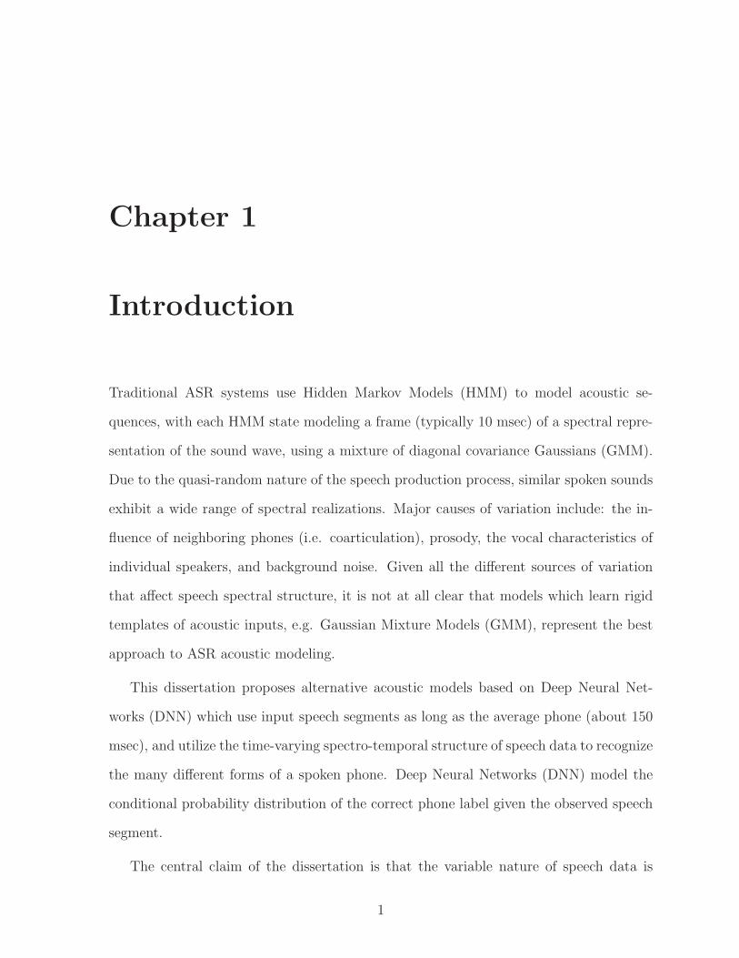
Chapter 1
Introduction
Traditional ASR systems use Hidden Markov Models (HMM) to model acoustic se-
quences, with each HMM state modeling a frame (typically 10 msec) of a spectral repre-
sentation of the sound wave, using a mixture of diagonal covariance Gaussians (GMM).
Due to the quasi-random nature of the speech production process, similar spoken sounds
exhibit a wide range of spectral realizations. Major causes of variation include: the in-
fluence of neighboring phones (i.e. coarticulation), prosody, the vocal characteristics of
individual speakers, and background noise. Given all the different sources of variation
that affect speech spectral structure, it is not at all clear that models which learn rigid
templates of acoustic inputs, e.g. Gaussian Mixture Models (GMM), represent the best
approach to ASR acoustic modeling.
This dissertation proposes alternative acoustic models based on Deep Neural Net-
works (DNN) which use input speech segments as long as the average phone (about 150
msec), and utilize the time-varying spectro-temporal structure of speech data to recognize
the many different forms of a spoken phone. Deep Neural Networks (DNN) model the
conditional probability distribution of the correct phone label given the observed speech
segment.
The central claim of the dissertation is that the variable nature of speech data is
1
Chapter 1. Introduction 2
better captured with deep neural network (DNN) acoustic models than with Gaussian
Mixture Models (GMM). The proposed DNN acoustic models have the flexibility neces-
sary to assimilate different spectro-temporal realizations of the same phone under various
conditions using higher level representations that marginalize out undesirable informa-
tion. Each layer of the DNN learns distributed representations of features presented at
the layer below where multiple experts (i.e. hidden units) collaborate together to explain
various hidden causes of input data. Such a representation allows the model to focus
more and more on aspects that are important for accurate ASR at deeper layers. Also,
the distributed nature of the model’s representation helps generalize better to unseen sit-
uations (e.g. different speakers, noise sources, and languages), even with limited amounts
of training data. By contrast, each expert (i.e. Gaussian) in a GMM models the whole
input feature vector which makes GMMs inefficient when there are multiple simultaneous
hidden causes, because a GMM requires a large number of Gaussian components to deal
with the cross-product of all the causes.
We, however, found that DNN acoustic models prefer features that smoothly change
both in time and frequency, like the log mel-frequency spectral coefficients (MFSC), to
the decorrelated mel-frequency cepstral coefficients (MFCC). MFSC features make it
easier for DNNs to discover linear relations as well as higher order causes of the input
data, leading to a better overall system performance.
Such slowly changing features along the frequency axis makes it possible to deal
explicitly with speaker variations in a manner similar to vocal tract length normalization
(VTLN) techniques using Convolutional Neural Networks (CNN). The convolution and
pooling operations of a CNN are performed along the frequency axis to spot local spectro-
temporal structures with tolerance for the small translations caused by the different vocal
tract lengths of different speakers.
Chapter 1. Introduction 3
1.1 Thesis structure
This thesis is organized as follows:
• Chapter 2 discusses previous ASR acoustic modeling efforts. The state-of-the-art
HMM/GMM system is presented as well as various enhancements related to speaker
and environment adaptation, covariance modeling, and the objective functions to
be optimized. The database used in this dissertation and the experimental setup
are also covered in this chapter.
• Chapter 3 presents layer-wise unsupervised feature learning for spoken data using
a stack of Restricted Boltzmann Machines (RBM) that are used to initialize a Deep
Neural Network (DNN). Each RBM learns a distributed representation of the input
from the layer below using an approximate maximum likelihood training algorithm
called Contrastive Divergence (CD). The resulting network is used as an initial
state for the fine tuning phase, which uses the backpropagation algorithm.
• Chapter 4 investigates the appropriate input feature representation for DNN acous-
tic models. The typical feature representation choice for diagonal covariance GMM
acoustic models, MFCCs, co-evolved with that model and therefore is not neces-
sarily the best choice for the very different DNN acoustic model.
• Chapter 5 investigates various ways of performing speaker adaptation, required for
higher ASR accuracy, in the context of DNN acoustic models. Speaker-adapted
input features are used and two new speaker adaptation techniques are presented
which have the flavor of eigenvoice speaker adaptation methods and do not require
extra speaker label information.
• Chapter 6 introduces a new acoustic model based on Convolutional Neural Networks
(CNN) which performs speaker normalization by convolving and pooling learned
filters along the frequency axis. It is motivated by the wide range of vocal tract
Chapter 1. Introduction 4
lengths across speakers. Deep CNN acoustic models achieved the best published
results over many small and large vocabulary tasks.
• Chapter 7 provides a brief summary of contributions made in the thesis and dis-
cusses future research directions.
1.2 Thesis contributions
This thesis introduces Deep Neural Networks (DNN) acoustic models for ASR. DNN
acoustic models outperform other previously proposed methods on various standard
benchmarks. It demonstrates the drawbacks of using Mel Frequency Cepstral Coeffi-
cients (MFCCs) rather than Mel Frequency spectral Coefficients (MFSCs) as the input
features for DNN acoustic models. Also, it presents a variety of speaker adaptation tech-
niques for DNN acoustic models. A new Convolutional Neural Networks (CNN) acoustic
model is introduce which performs speaker normalization by acting along the frequency
axis achieving the best published results to date on various large vocabulary tasks.
Chapter 2
Background and experimental setup
2.1 Past and current research trends in acoustic mod-
eling
2.1.1 A basic HMM/GMM system for ASR
A typical ASR system represents the speech signal with Mel Frequency Cepstral Coeffi-
cients (MFCC) which are computed every 10 ms using an overlapping analysis window of
around 25 ms. MFCCs are generated by applying a discrete cosine transformation (DCT)
to a log spectral estimate computed by smoothing an FFT with around 20 frequency bins
distributed non-linearly (on a mel scale) across the speech spectrum to approximate the
frequency response of the human ear.
Hidden Markov Models (HMMs) are used to model the MFCC observation sequence.
The HMM, which is a special case of the regular Markov model, has a sequence of state
transitions that are not directly visible. However, the HMM output observations are
visible and are used to infer the hidden state sequence. Each HMM state is modeled by
a Gaussian mixture model (GMM) with many diagonal covariance Gaussians which are
cheaper to train compared to full covariance Gaussians of the same size. MFCCs are a
5
Chapter 2. Background and experimental setup 6
good fit to this framework because they have been already decorrelated by the DCT.
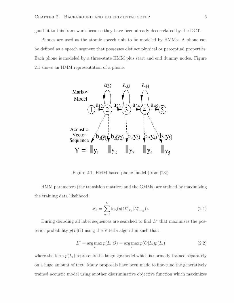
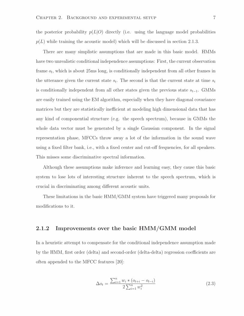
Phones are used as the atomic speech unit to be modeled by HMMs. A phone can
be defined as a speech segment that possesses distinct physical or perceptual properties.
Each phone is modeled by a three-state HMM plus start and end dummy nodes. Figure
2.1 shows an HMM representation of a phone.
Figure 2.1: HMM-based phone model (from [23])
HMM parameters (the transition matrices and the GMMs) are trained by maximizing
the training data likelihood:
FL =N∑
n=1
log(p(On1:Tn
|Ln1:mn
)). (2.1)
During decoding all label sequences are searched to find L∗ that maximizes the pos-
terior probability p(L|O) using the Viterbi algorithm such that:
L∗ = argmaxi
p(Li|O) = argmaxi
p(O|Li)p(Li) (2.2)
where the term p(Li) represents the language model which is normally trained separately
on a huge amount of text. Many proposals have been made to fine-tune the generatively
trained acoustic model using another discriminative objective function which maximizes
Chapter 2. Background and experimental setup 7
the posterior probability p(L|O) directly (i.e. using the language model probabilities
p(L) while training the acoustic model) which will be discussed in section 2.1.3.
There are many simplistic assumptions that are made in this basic model. HMMs
have two unrealistic conditional independence assumptions: First, the current observation
frame ot, which is about 25ms long, is conditionally independent from all other frames in
the utterance given the current state st. The second is that the current state at time st
is conditionally independent from all other states given the previous state st−1. GMMs
are easily trained using the EM algorithm, especially when they have diagonal covariance
matrices but they are statistically inefficient at modeling high dimensional data that has
any kind of componential structure (e.g. the speech spectrum), because in GMMs the
whole data vector must be generated by a single Gaussian component. In the signal
representation phase, MFCCs throw away a lot of the information in the sound wave
using a fixed filter bank, i.e., with a fixed center and cut-off frequencies, for all speakers.
This misses some discriminative spectral information.
Although these assumptions make inference and learning easy, they cause this basic
system to lose lots of interesting structure inherent to the speech spectrum, which is
crucial in discriminating among different acoustic units.
These limitations in the basic HMM/GMM system have triggered many proposals for
modifications to it.
2.1.2 Improvements over the basic HMM/GMM model
In a heuristic attempt to compensate for the conditional independence assumption made
by the HMM, first order (delta) and second-order (delta-delta) regression coefficients are
often appended to the MFCC features [20]:
∆ot =
∑n
i=1wi ∗ (ot+i − ot−i)
2∑n
i=1w2i
(2.3)
Chapter 2. Background and experimental setup 8
where n is the regression window width and wi are the regression coefficients. Delta-delta
parameters (∆2ot) are derived in the same way starting from the delta features. So the
new feature vector is:
onewt = [oTt ∆oTt ∆2oTt ]T . (2.4)
The temporal differences also assist diagonal covariance Gaussians in modelling the
strong temporal covariances in the signal by reducing these particular pairwise covari-
ances to individual coefficients. By variance normalization of input features, these dif-
ferences got exaggerated which help improve recognition performance. On the other
hand, it models only short term dependencies without explicit modeling of longer term
trajectories [15].
As mentioned in section 2.1.1, HMM-based recognizers do not usually include any
explicit modeling of correlations between different dimensions in the feature vector, i.e.,
conditioned on the hidden states, acoustic features are modeled by Gaussian distributions
with diagonal covariance matrices. This is because it is cheaper both in running time
and in the amount of data required (for each Gaussian) than reliably estimating the full
covariance matrices.
Factor analysis has been proposed to model the correlations between acoustic features
[87]. The idea behind factor analysis is to map systematic variations of the data into a
lower dimensional subspace. This enables one to approximate, in a very compact way,
the full covariance matrices for high dimensional data. These matrices are expressed in
terms of a small number of parameters that model the most significant correlations.
Let x ∈ RD be a feature whose covariance we want to model, and which is normally
distributed with mean µ, and let z ∈ Rf be a Gaussian latent factor that generates x,
where f ≪ D. So the probability density of p(x|z) is also Gaussian with mean µ+Λz and
diagonal covariance ψ where Λ is the factor loading matrix that relates the hidden factor
z to the observations x. Marginalizing out z, the probability density of x under the factor
analysis model is Gaussian with mean µ and covariance ψ+ΛΛT . This model allows for
Chapter 2. Background and experimental setup 9
modeling the important correlations between features using only D + Df variables per
Gaussian component rather than D2 variables.
It follows that when the diagonal elements of ψ are small, most of the variation in x
occurs in the subspace S(Λ) spanned by the columns of Λ. The variances ψii measure
the typical size of component-wise fluctuations outside this subspace.
[87], used filter bank outputs as input features for x, which are strongly correlated,
while [80] used MFCCs as features which, although they are decorrelated by the DCT,
have non-zero off-diagonal elements in their covariance matrices. Improvements were
introduced by sharing covariances between Gaussian components and using a GMM to
model the latent variable z [80]. Further improvements were achieved by modeling the
precision matrix [91] rather than the covariance matrix so that no inversion was needed
during decoding.
The precision matrix can be approximated as, [24, 91]:
Σ−1m =
B∑
i=1
νmiSi (2.5)
where νm is a Gaussian-component-specific weight vector that specifies the contribu-
tion from each of the B global positive semi-definite matrices. Further refinement takes
B to be the number of dimensions with symmetric basis matrices that have rank 1 so
that Si = aTi ai where ai is the ith row of the matrix A:
Σ−1m =
d∑
i=1
νmiaTi ai = AΣ
(m)−1diag AT . (2.6)
Σ(m)diag is specific to each component whereas the A matrices are shared between many
components.
As discussed earlier, HMMs use a single-state variable to encode all state informa-
tion (typically, just the identity of the current phonetic unit) while Dynamic Bayesian
Networks (referred to here as “DyBNs”), a generalization of HMMs, provide a conve-
nient method for defining acoustic models that maintains an explicit representation of
Chapter 2. Background and experimental setup 10
the speech articulators (e.g. lips, tongue, jaw, etc...) as they change over time. They can
therefore naturally handle coarticulation effects [99]. In addition, dependencies between
multiple acoustic features could be modeled to relax the strong independence assumption
of HMMs, which makes DyBNs more accurate models for speech recognition and gen-
eration [9]. As the DyBN becomes more powerful, by introducing connections between
its hidden states to encode dependencies, learning becomes harder as the exact inference
of the hidden variables becomes intractable, so variational and approximate inference
models are used in such complex models [27].
2.1.3 Discriminative objective functions for training GMMs
Many proposals have been made to fine-tune generatively trained acoustic models using
another discriminative objective function that maximizes the posterior probability p(L|O)
directly and is directly related to the performance metric, e.g., word error rates (WER).
Using Bayes’ rule, the posterior probability of the correct label sequence Lc is
p(Lc|O) =p(O|Lc)p(Lc)∑
l p(O|l)p(l)(2.7)
where the summation in the denominator is over all possible label sequences. In practice
this summation is performed over only strong competing sequences (they are represented
either in a lattice or an N-best list). The language model probabilities p(l) are normally
fixed while optimizing the acoustic model parameters. This family of training methods
is harder to optimize than ML because they include all other competing models, i.e.,
it is a joint optimization of many models that constrain each other. Discriminative
objectives are prone to overfitting unless coupled with another generative objective as a
regularizer [70].
Maximum Mutual Information (MMI) training [6, 75] tries to maximize the mutual
information between the training data and the correct label sequence:
Chapter 2. Background and experimental setup 11
I(L,O) = H(L)−H(L|O)
=∑
l
∑
o
p(l, o) log(p(l, o)
p(l)p(o))
≈1
N
N∑
n=1
log(p(L|O))
FMMI =N∑
n=1
log(p(On|Ln)
κp(Ln)∑
l p(On|l)κp(l)) (2.8)
where κ is a smoothing factor (κ < 1.0) to make less likely sequences contribute to the
objective function, make the objective more smoothly differentiable, and improve model
generalization. The expectation in the second equation was approximated by averaging
over all the training data samples N and dropping the label entropy term. MMI training,
while being well-motivated from an information-theoretic prospective, does not relate
directly to the required performance metric, e.g., word error rates (WER).
The Minimum phone error training (MPE) objective function directly optimizes
weighted phone transcription accuracy [78]:
FMPE =N∑
n=1
∑
u
p(u|On)A(u, un)
=N∑
n=1
∑
u p(On|u)κp(u)A(u, un)
∑
l p(On|l)κp(l)(2.9)
where A(u, un) is the raw phone transcription accuracy of the sequence u given the
reference sequence un (which equals the number of reference phones minus the number
of errors).
Even when overall system performance is measured by Word Error Rate (WER),
maximizing the phone transcription accuracy (the edit distance on the phone level) has
been found to be more helpful than directly maximizing word transcription accuracy (the
edit distance on the word level) [78].
Chapter 2. Background and experimental setup 12
Another proposal is Large Margin training (LM). The main idea here is to maximize
the classification margin [48, 90], i.e., to separate the correct versus incorrect label se-
quences by margins proportional to the number of mislabeled units like phones or words,
while using a convex objective function to avoid local minima.
We define D(O,L) as:
D(O,L) =∑
t
(λ(lt−1, lt) + ρ(ot, lt)) (2.10)
where λ and ρ are state transition and state output score functions respectively.
The set of constraints that the model should satisfy are:
D(On, Ln)−D(On, U) ≥ H(Ln, U), ∀U 6= Ln
−D(On, Ln) + log∑
U 6=Ln
exp(D(On, U) +H(Ln, U)) ≤ 0 (2.11)
where H() is the hamming distance between two sequences. The objective function
becomes:
FLM = γ∑
c,m
trace(φcm) +N∑
n=1
[−D(On, Ln) + log∑
U 6=Ln
exp(D(On, U) +H(Ln, U))]+,
subject to the positive semidefinite constraints φjm > 0 (2.12)
where φcm is a matrix containing the parameters of the Gaussian mixture m for state
c. [a]+ is a hinge function which equals zero unless a > 0, in which case it equals a.
Affected by the success of the large margin training of HMMs, The MMI objective
was changed to have a large margin flavour in Boosted maximum mutual information
training (BMMI) [76]:
FBMMI =N∑
n=1
logp(On|Ln)
κp(Ln)∑
l p(On|l)κp(l)exp(−bA(l, Ln))(2.13)
where A() is the raw phone transcription accuracy. In this objective function, the likeli-
hood of the sentences that have more errors is emphasized to enforce a soft margin that is
Chapter 2. Background and experimental setup 13
proportional to the number of errors in a hypothesized sentence. The objective is related
to the MPE objective with no consistent superiority in performance [76].
Following the success of using the MPE and BMMI objective functions for training
HMMs, the same objectives have been proposed for training acoustic features [76, 77]
so that they are more discriminative. The first stage is to project the low (e.g. 39)
dimensional features into high (e.g. 100,000) dimensional ones. A set of Gaussians is
created by likelihood-based clustering in the acoustic space, each frame being represented
by its sparse Gaussian responsibility vector. Then a contextual window (e.g. 7 frames of
context) of these high-dimensional vectors is formed into the vector ht. The new features
yt are:
yt = xt +Mht (2.14)
where the matrixM projects back the high-dimensional vector ht into the original feature
space. The main work is in training the matrix M using an MPE or BMMI objective
function.
2.1.4 Speaker adaptation
There are a few terms related to adapting acoustic models that need clarification. A
speaker-independent (SI) model is one created using utterances from many speakers
which contain both intraspeaker (within the same speaker) and interspeaker (between
different speakers) variabilities. A speaker-dependent (SD) model is one created using
utterances recorded from one speaker only which, when practical, contains intraspeaker
variations only. For applications in which there will be only one speaker interacting with
the ASR system, e.g., a dictation system, ideas have been proposed to adapt an existing
SI model to one test speaker, e.g., the one who will be using the dictation system, during
an enrollment session to ensure the best performance for this speaker. After collecting
speaker data, a speaker transformation is created, called speaker profile, which shifts the
SI model closer to this speaker’s point in the acoustic space [96].
Chapter 2. Background and experimental setup 14
Building on that idea, pre-existing transforms are built a priori using data clustered
based on speaker similarity so that, during decoding, every utterance is mapped to the
closest cluster. The cluster’s transform is then used for very fast adaptation.
The idea of speaker adaptation has also been used during training where, as opposed
to SI models, every utterance in the training data is normalized (moved from its speaker
point in the acoustic space to a certain canonical speaker point) before building the
acoustic model so that the resulting training data, while keeping the intraspeaker varia-
tions, will not contain interspeaker differences. This is called speaker-adaptive training
(SAT) [4] which offers a more practical alternative to SD models which are then adapted
during test time to match test speakers. One major drawback of the proposed adaptation
techniques is that they are performed separately from GMM training, which sometimes
cause a degradation of performance. A better method would train the GMM and speaker
transforms jointly to reduce WER.
One major source of interspeaker variability is the variation of vocal-tract shape
among speakers. The spectral formant peaks are related to the length of the vocal
tract and the formant center frequencies can vary by as much as 25% between speakers.
Systems that use MFCCs as their features will not be able to recover the missing data
from mislocated filter banks. One basic solution to this problem is to warp the spectrum
so that we have normalized features with speaker-specific vocal-tract length information
removed [5, 17, 61]. For training, given a set of HMM models λ, a grid search is done to
choose the optimal linear warping frequency factor α∗i for each speaker i which maximizes
the data likelihood:
α∗i = argmax
α
p(Oαi |λ, Li) (2.15)
where Oαi are the warped features using the factor α. A new HMM model is created
using the new warped features and then the whole process is repeated until the warping
factor stabilizes. For testing, a first-pass decoding finds approximate labels then, α is
Chapter 2. Background and experimental setup 15
selected to warp the input features for this utterance before the final decoding. An
improved version uses a piece-wise linear function [32] for warping the spectrum.
Maximum likelihood linear regression (MLLR) adaptation applies a linear transfor-
mation to the learned model parameters to improve system performance for a certain test
speaker s by transforming the model means and covariances to maximize the likelihood
of the test data under the new model [21,62]. If µm and Σm are the mean and covariance
of the Gaussian m, then:
µsm = Asµm + bs
Σsm = HsΣmHsT (2.16)
where µsm and Σsm are the mean and covariance of the Gaussianm adapted to speaker
s. To perform adaptation with as little data as possible, all Gaussians in the system are
pooled together in a tree so that Gaussians that are closer in the acoustic space will share
the same linear transforms. As the amount of data available for speaker s increases, we
descend deeper into the tree to have more specific transformations of the Gaussians. If
we constrain the mean and covariance transforms to be the same:
µsm = Ascµ
m + bsc
Σsm = AscΣ
mAsTc (2.17)
it can be shown also that:
Os = AsO + bs (2.18)
where:
As = inv(Asc)
bs = −inv(Asc)b
sc. (2.19)
Chapter 2. Background and experimental setup 16
This is called Constrained MLLR (CMLLR) or Feature-space MLLR (fMLLR) [21] where
the learned transformation could be applied directly in the feature space.
During the estimation of both MLLR and CMLLR, an adaptation-data transcript
is needed. Thus we may distinguish between a supervised adaptation mode where the
transcript is known a priori (e.g. user enrollment in voice enabled software) and an
unsupervised adaptation mode where the adaptation-data transcript should be provided
with one pass of the recognizer using an existing acoustic model before the transform is
estimated (this process is repeated until convergence) [95].
As mentioned in section 2.1.1, the failure of GMMs to model componential structure in
the data requires MLLR to have many transforms (which requires a lot of more adaptation
data) to model the huge number of Gaussians used in such systems.
For Speaker-independent (SI) systems, acoustic model parameters are estimated using
a large number of speakers, which is less accurate than Speaker-dependent (SD) acoustic
models where the training data is collected from only one speaker. Spectral variations in
SI models are caused by interspeaker variability, e.g., the anatomy of the vocal tract and
the vocal cords, by regional dialects and by speaking style, in addition to phonetically
relevant sources of variation. As a result, the SI spectral distributions often have higher
variance than the corresponding SD distributions and hence higher overlap among differ-
ent speech units. In Speaker Adaptive Training (SAT) [4], these two sources of variation
are separated by explicit MLLR transformations modeled jointly with the GMM den-
sity estimation so that one focuses on speaker variations and the other on phonetically
relevant variations of the speech signal.
Another formulation of SAT can be reached by using the CMLLR idea where speaker
adaptation take place in the feature domain rather than in the model domain. In [21],
training data from different speakers are transformed to a canonical speaker feature space
where interspeaker variability is removed and then a new HMM/GMMmodel is estimated
in this space, which focuses on the intraspeaker variability only.
Chapter 2. Background and experimental setup 17
The speaker-adaptation process when applied in the test phase is a compromise be-
tween the correctness of the estimated adapted model (Which benefits from more data)
and how fast the enrollment/adaptation phase is. Some speaker adaptation techniques
arrange training speakers in a tree based on their gender and speaker rate with a separate
HMM/GMM model built for each leaf node in the tree. So during the test phase, a new
test speaker is quickly assigned to one leaf cluster and its model is used [36].
Furthermore, every test speaker can be represented as a weighted sum of previously
trained speaker cluster HMM/GMMs [25, 36]. So the mean of certain Gaussians for
speaker s is:
µs =C∑
c=1
λcsµc (2.20)
where µc is a Gaussian in the GMM of cluster c, C is the total number of clusters,
and the λ vector contains the speaker specific mixing proportions. The λ parameters are
trained using ML.
2.1.5 Neural networks for ASR
Feedforward neural networks NN have been used in many ASR systems [8,10,73] because
they offer several potential advantages over GMMs:
• Their estimation of the posterior probabilities of HMM states does not require
detailed assumptions about the data distribution.
• They allow an easy way of combining diverse features, including both discrete and
continuous features.
• They use far more of the data to constrain each parameter because the output on
each training case is sensitive to a large fraction of the weights.
It is harder to train a neural network model using gradient descent on mini-batches than
it is to fit a GMM using EM, and there are usually more decisions to be made about meta-
parameters such as learning rates and regularization terms. The use of special-purpose
Chapter 2. Background and experimental setup 18
hardware with multiple DSP chips by [72] led to a large reduction in the training time
needed for neural nets and helped make neural networks competitive with GMMs for
speech recognition.
Conditioned on an acoustic feature vector, NNs provide the posterior probability
distribution over the class labels. In a hybrid HMM-NN model [10], the posterior proba-
bilities are fed to a Viterbi decoder to produce word sequences (i.e. the NN replaces the
GMM component). In the Tandem model [37], the decorrelated log posterior probabil-
ities (sometimes augmented with MFCC features) are fed as feature vectors to a basic
HMM/GMM system so that it compromises between the high modeling power of NNs
and all of the algorithms and tools developed for GMMs.
Recurrent neural networks (RNNs) have been also applied to ASR in the same way
that the hybrid system works [79]. The advantage of the RNN is that the previous
hidden state vectors of the network are used along with the current input features to
determine the current hidden state vector which makes RNNs a very powerful model for
time sequences. RNNs are harder to train than feed forward NNs with only a few hidden
layers because, as when they are unfolded in time, they correspond to a deep network
with T layers, where T is the sequence length.
In the previously mentioned NN systems, the input acoustic feature vector is a context
window of n MFCC frames (with 10 ms frame shift) which covers 10 ∗ n ms of the input
speech (i.e. features are 10 ∗ n ms thick vertical slices from the MFCC spectrogram that
covers all the frequency bands). In the TRAPS architecture [40], features are horizontal
slices such that each one focuses on one frequency band (could be more than one band)
for about 1sec. A band filter is a NN that keeps focusing on one horizontal slice over time
to produce a posterior probability distribution over class labels. Many band filters, e.g.,
15, are then combined using the output NN to produce the final posterior probability dis-
tribution for each frame which could be used in hybrid or tandem systems. The TRAPS
architecture provides robust frame accuracies in noisy conditions because decisions are
Chapter 2. Background and experimental setup 19
made reliably by some band filters even if others are corrupted by band-limited noise.
This architecture is inspired by human speech recognition findings, as shown in the next
section.
2.1.6 Human speech recognition
Thinking of biological systems as the ultimate information processors, many studies
have been performed to understand how humans perceive, process and recognize speech
[3, 19, 31]. Human speech recognition (HSR) is believed to be largely bottom-up, where
speech is recognized based on a hierarchy of feature layers that use progressively longer
contexts. Feature extractors and event detectors start from the filters in the cochlea. As
we go higher in the hierarchy, more context is integrated, leading to a decrease in entropy
and the appearance of more abstract representations (e.g. phones, syllables, words,etc
...) [3].
Existing automated speech recognition systems do not work the way humans work.
This is because automatic speech recognition (ASR) uses spectral templates, while hu-
mans work with partial (i.e. local) recognition information across frequencies (e.g., for-
mants). It has been shown in humans, for example, that forcing partial recognition errors
in one frequency region does not affect partial recognition at other frequencies, i.e., the
partial recognition errors across frequency are independent [3]. It seems to be this local
feature-processing, uncoupled across frequency, that makes human speech recognition
(HSR) robust to noise and reverberation. These extracted features are then integrated
into basic sound units (phones), and the phones are then grouped into syllables, then
words, and so forth [3].
HSR studies show that current ASR systems, while good for some tasks, are too
shallow and model human processing of speech poorly. The work in [64] compares the
performance of humans and speech recognizers using six modern speech corpora with
vocabularies ranging from 10 to 65,000 words. Error rates of machines are often more
Chapter 2. Background and experimental setup 20
than an order of magnitude greater than those of humans for quiet, clearly spoken speech.
Machine performance degrades by a larger margin below that of humans in noisy condi-
tions. Human performance remains high with natural variability caused by new speakers,
spontaneous speaking styles, noise, and reverberation. Human performance also remains
high with unnatural degradation caused by waveform clipping, band-reject filtering, and
analog waveform scrambling.
2.1.7 Segmental and landmark based methods
Many speech scientists believe that the acoustic cues important for phonetic contrasts are
best characterized in relation to specific temporal landmarks in the speech signal, such as
points of oral closure or release, or other points of maximal constriction or opening in the
vocal tract which are produced during speech production [29]. Many of these locations
correspond to phonetic boundaries, leading some speech researchers to consider segment-
and landmark-based approaches for ASR. Work in [35] recognizes different streams of
phonological features (e.g. voice, manner, and place of articulation) and uses these
temporal landmarks to synchronize between them.
The work in [47] proposes a hierarchical framework where each layer is designed to
capture a set of distinctive feature landmarks. For each feature, a specialized acoustic
representation is constructed in which that feature is easy to detect.
The “SUMMIT” speech recognizer [98] used a segment-based framework for its acoustic-
phonetic representation of the speech signal. The observation space takes the form of a
graph where different paths through the graph are associated with different sets of fea-
ture vectors. During decoding, proper normalization of likelihoods is needed as different
paths through the graph compute likelihoods on different observation spaces.
Chapter 2. Background and experimental setup 21
2.2 Experimental Setup
In this section the database and the experimental setup used in the reminder of the thesis
are described.
2.2.1 TIMIT corpus
Phone recognition experiments were performed on the TIMIT corpus.1 We used the 462
speaker training set and removed all SA records (i.e., identical sentences for all speakers
in the database) since they could bias the results. A separate validation set of 50
speakers, as defined in [34], was used for testing all of the meta-parameters.
Results are then reported using the 24-speaker core test set, which is different
from the validation set. Running Multiple rounds of cross-validation was not
necessary given that the validation set is not part of the training data, and
the training data size is sufficiently large.
The speech was analyzed using a 25-ms Hamming window with a 10-ms fixed frame
rate. In most of the experiments, we represented the speech using 12th-order Mel fre-
quency cepstral coefficients (MFCCs) and energy, along with their first and second tem-
poral derivatives. For other experiments, we used a Fourier-transform-based filter-bank
with 40 coefficients distributed on a mel-scale (and energy) together with their first and
second temporal derivatives (MFSC).
The data were normalized so that, averaged over the training cases, each coefficient,
first derivative, and second derivative had zero mean and unit variance. We used 183
target class labels, i.e., 3 states for each one of the 61 phones. After decoding, the
61 phone classes were mapped to a set of 39 classes as in [60] for scoring. All of our
experiments used a bigram language model over phones, estimated from the training set.
1http://www.ldc.upenn.edu/Catalog/CatalogEntry.jsp?catalogId=LDC93S1.
Chapter 2. Background and experimental setup 22
2.2.2 Computational setup
The acoustic models proposed in this thesis are quite computationally expensive. Train-
ing was accelerated by exploiting graphics processors, in particular GPUs in an NVIDIA
Tesla S1070 system, using the CUDAMAT library [69].
Chapter 3
Generatively trained DNN for
acoustic modeling
The state-of-the-art Automatic Speech Recognition (ASR) system, for many decades, has
used Hidden Markov Models (HMMs) to model the sequential structure of speech signals,
with local spectral variability modeled using mixtures of Gaussian densities. Until re-
cently, Feedforward neural networks have been also used in many ASR systems [8,10,73]
but with limited success compared to GMMs. In this chapter we propose revisiting
neural networks with two important modifications. First, the network weights are gener-
atively pretrained to maximize the data likelihood before applying the backpropagation
algorithm in a fine tuning phase. This way, the training process of neural networks is
closer to how GMMs are normally trained in ASR systems where they are trained first to
maximize the data likelihood then a discriminative training objective is used to improve
GMM recognition performance. Second, the network structure is extended to have many
hidden layers with each hidden layer containing many more hidden units than the usual
neural networks that have been applied to acoustic modeling in the past. This deep neu-
ral network acoustic model is the current state-of-the-art for ASR. This chapter is divided
into two sections that align with these two directions for acoustic modeling: generative
23
Chapter 3. Generatively trained DNN for acoustic modeling 24
training of neural networks and building deep networks. For each section, the main idea
is first motivated and presented, then evaluated on the TIMIT phone recognition task 1.
3.1 Generative training of one-hidden-layer neural
network acoustic models
3.1.1 Motivation
Previous applications of the neural network (NN) approach for acoustic modeling have
used the backpropagation algorithm to train the neural networks discriminatively. These
approaches coincide nicely with a trend initiated by [11] in which generative modeling is
replaced by discriminative training.
Discriminative models have one major disadvantage, that is, the amount of constraint
each data point imposes on the parameters of the model equals the number of bits
required to specify the correct label for the data point. For generative models, the
amount of constraint equals the number of bits required to describe the observed data
point itself. So when the input data vectors contain much more structure than the labels,
a generative model can learn many more parameters before it overfits. The benefit of
learning a generative model is greatly magnified when there is a large supply of unlabeled
speech in addition to the training data that have been labeled.
Generative pretraining of NNs is achieved using Restricted Boltzmann Machines
(RBMs) [44]. An RBM is a bipartite graph in which visible units that represent ob-
servations are connected to hidden units using undirected weighted connections. The
hidden units learn non-linear features that allow the RBM to model the statistical struc-
ture in the vectors of visible states.
1The TIMIT dataset turned out to be quite a good predictor of LVCSR performance.
Chapter 3. Generatively trained DNN for acoustic modeling 25
3.1.2 Restricted Boltzmann Machines (RBMs)
An RBM is a particular type of Markov Random Field (MRF) that has one layer of
stochastic visible units and one layer of stochastic hidden units. An RBM is restricted
in the sense that there are no visible-visible or hidden-hidden connections. In the sim-
plest type of RBM, the binary RBM, both the hidden and visible units are binary and
stochastic. To deal with real-valued input data, we use a Gaussian-Bernoulli RBM in
which the hidden units are binary but the input units are linear with Gaussian noise. We
will explain the Gaussian-Bernoulli RBM later after first explaining the simpler binary
RBM.
In a binary RBM, the weights on the connections and the biases of the individual
units define a probability distribution over the joint states of the visible and hidden units
using an energy function. The energy of a joint configuration is:
E(v,h|θ) = −V∑
i=1
H∑
j=1
wijvihj −V∑
i=1
bivi −H∑
j=1
ajhj (3.1)
where θ = (w,b, a), wij represents the symmetric interaction term between visible unit
i and hidden unit j, and bi and aj are their bias terms. V and H are the numbers of
visible and hidden units.
The probability that an RBM assigns to a visible vector v is:
p(v|θ) =
∑
h e−E(v,h)
∑
u
∑
h e−E(u,h)
. (3.2)
Since there are no hidden-hidden connections, the conditional distribution p(h|v, θ) is
factorial and is given by:
p(hj = 1|v, θ) = σ(aj +V∑
i=1
wijvi) (3.3)
where σ(x) = (1 + e−x)−1. Similarly, since there are no visible-visible connections, the
conditional distribution p(v|h, θ) is factorial and is given by:
p(vi = 1|h, θ) = σ(bi +H∑
j=1
wijhj). (3.4)
Chapter 3. Generatively trained DNN for acoustic modeling 26
Exact maximum likelihood learning is infeasible in a large RBM because it is expo-
nentially expensive to compute the derivative of the log probability of the training data.
Nevertheless, RBMs have an efficient approximate training procedure called “contrastive
divergence” [42] which makes them suitable as building blocks for learning DNNs. We
repeatedly update each weight, wij, using the difference between two measured, pairwise
correlations:
∆wij ∝ 〈vihj〉data − 〈vihj〉recon.. (3.5)
The first term on the right hand side of Eq. 3.5 is the measured frequency with which
visible unit i and hidden unit j are on together when the visible vectors are samples
from the training set and the states of the hidden units are determined by Eq. 3.3. The
second term is the measured frequency with which i and j are both on when the visible
vectors are “reconstructions” of the data vectors and the states of the hidden units are
determined by applying Eq. 3.3 to the reconstructions. Reconstructions are produced by
applying Eq. 3.4 to the hidden states that were computed from the data when computing
the first term on the right hand side of Eq. 3.5.
For Gaussian-Bernoulli RBMs the energy of a joint configuration is:
E(v,h|θ) =V∑
i=1
(vi − bi)2
2−
V∑
i=1
H∑
j=1
wijvihj −H∑
j=1
ajhj. (3.6)
To keep the equation simple, we assume that the Gaussian noise level of all the visible
units is fixed at 1. We also normalize the input data to have a fixed variance of 1 for
each component over the whole training set.
Since there are no visible-visible connections, the conditional distribution p(v|h, θ) is
factorial and is given by:
p(vi|h, θ) = N
(
bi +H∑
j=1
wijhj, 1
)
(3.7)
where N (µ, V ) is a Gaussian with mean µ and variance V . Apart from these differences,
the inference and learning rules for a Gaussian-Bernoulli RBM are the same as for a
binary RBM, though, in practice, the learning rate needs to be smaller.
Chapter 3. Generatively trained DNN for acoustic modeling 27
W
h
…..…
v tv (t-n/2) v (t-n/2) lt
(a) RBM
W
h
v t
……
v(t-1)v(t-n)
A(t-1)
A(t-n)
B(t-1)
B(t-n)
l t
(b) CRBM
W
h
v t
……
v(t+n/2)v(t-n/2)
A(t+n/2)A(t-n/2)
B(t+n/2)B(t-n/2)
……
l t
(c) ICRBM
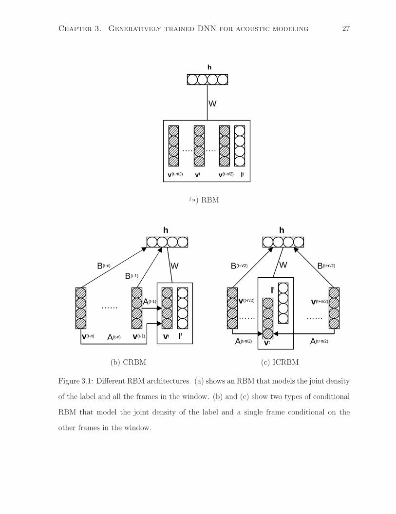
Figure 3.1: Different RBM architectures. (a) shows an RBM that models the joint density
of the label and all the frames in the window. (b) and (c) show two types of conditional
RBM that model the joint density of the label and a single frame conditional on the
other frames in the window.
Chapter 3. Generatively trained DNN for acoustic modeling 28
3.1.3 The conditional RBM
The Conditional RBM (CRBM) [93] is a variant of the standard RBM that models
vectors of sequential data by considering the visible variables in previous time steps as
additional, conditioning inputs. Two types of directed connections are added; autore-
gressive connections from the past n frames of the visible vector to the current visible
vector, and connections from the past n frames of the visible vector to the hidden units
as in figure (3.1-b). Given the data vectors at times t, t − 1, ..., t − n the hidden units
at time t are conditionally independent. One drawback of the CRBM is that it ignores
future frames when inferring the hidden states, so it does not do backward smoothing.
Performing backward smoothing correctly in a CRBM would be intractable because, un-
like an HMM, there are exponentially many possible hidden state vectors, so it is not
possible to work with the full distribution over hidden vectors when the hidden units are
not independent.
If we are willing to give up on the ability to generate data sequentially from the model,
the CRBM can be modified to have both autoregressive and visible-hidden connections
from a limited set of future frames as well as from a limited past. So we get the interpo-
lating CRBM (ICRBM) [figure (3.1-c)]. The directed, autoregressive connections from
temporally adjacent frames ensure that the ICRBM does not waste the representational
capacity of the non-linear hidden units by modeling aspects of the central frame that can
be predicted linearly from the adjacent frames.
3.1.4 Application to phone recognition
A context window of successive frames of feature vectors is used to set the states of the
visible units of the RBM. To train the RBM to model the joint distribution of a set of
frames and the L possible phone labels of the last or central frame, we add an extra
“softmax” visible unit that has L states, one of which has value 1. The energy function
Chapter 3. Generatively trained DNN for acoustic modeling 29
becomes:
E(v, l,h; θ) = −V∑
i=1
H∑
j=1
wijhjvi −L∑
k=1
H∑
j=1
wkjhjlk −H∑
j=1
ajhj −L∑
k=1
cklk +V∑
i=1
(vi − bi)2
2
(3.8)
p(lk = 1|h; θ) = softmax(H∑
j=1
wkjhj + ck). (3.9)
And, p(l|v) can be computed exactly using:
p(l|v) =
∑
h e−E(v,l,h)
∑
l
∑
h e−E(v,l,h)
. (3.10)
The value of p(l|v) can be computed efficiently by utilizing the fact that the hidden
units are conditionally independent. This allows the hidden units to be marginalized out
in a time that is linear in the number of hidden units. To generate phone sequences, the
values of log p(l|v) per frame are fed to a Viterbi decoder.
Following the Contrastive Divergence (CD) approximation to the gradient of the joint
likelihood function of data and labels, the update rule for the visible-hidden weights is:
∆wij = 〈vihj〉data − 〈vihj〉recon.. (3.11)
The update rule for the autoregressive visible-visible links is:
∆A(t−q)ij = v
(t−q)i (〈vtj〉data − 〈vtj〉recon.) (3.12)
where A(t−q)ij is the weight from unit i at time (t− q) to unit j. For the visible-hidden
directed links it is:
∆B(t−q)ij = v
(t−q)i (〈htj〉data − 〈htj〉recon.). (3.13)
Chapter 3. Generatively trained DNN for acoustic modeling 30
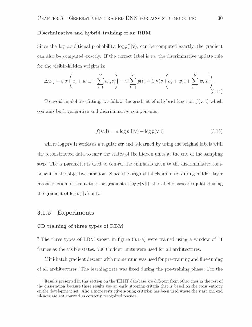
Discriminative and hybrid training of an RBM
Since the log conditional probability, log p(l|v), can be computed exactly, the gradient
can also be computed exactly. If the correct label is m, the discriminative update rule
for the visible-hidden weights is:
∆wij = viσ
(
aj + wjm +V∑
i=1
wijvi
)
− vi
L∑
k=1
p(lk = 1|v)σ
(
aj + wjk +V∑
i=1
wijvi
)
.
(3.14)
To avoid model overfitting, we follow the gradient of a hybrid function f(v, l) which
contains both generative and discriminative components:
f(v, l) = α log p(l|v) + log p(v|l) (3.15)
where log p(v|l) works as a regularizer and is learned by using the original labels with
the reconstructed data to infer the states of the hidden units at the end of the sampling
step. The α parameter is used to control the emphasis given to the discriminative com-
ponent in the objective function. Since the original labels are used during hidden layer
reconstruction for evaluating the gradient of log p(v|l), the label biases are updated using
the gradient of log p(l|v) only.
3.1.5 Experiments
CD training of three types of RBM
2 The three types of RBM shown in figure (3.1-a) were trained using a window of 11
frames as the visible states. 2000 hidden units were used for all architectures.
Mini-batch gradient descent with momentum was used for pre-training and fine-tuning
of all architectures. The learning rate was fixed during the pre-training phase. For the
2Results presented in this section on the TIMIT database are different from other ones in the rest ofthe dissertation because these results use an early stopping criteria that is based on the cross entropyon the development set. Also a more restrictive scoring criterion has been used where the start and endsilences are not counted as correctly recognized phones.
Chapter 3. Generatively trained DNN for acoustic modeling 31
fine-tuning phase, an early stopping criterion that is based on the cross entropy on the
development set was used along with learning rate annealing. Training stops when the
learning rate falls below a certain threshold.
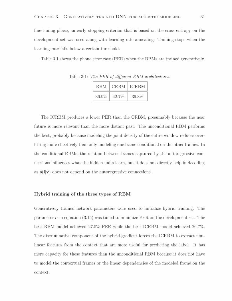
Table 3.1 shows the phone error rate (PER) when the RBMs are trained generatively.
Table 3.1: The PER of different RBM architectures.
RBM CRBM ICRBM
36.9% 42.7% 39.3%
The ICRBM produces a lower PER than the CRBM, presumably because the near
future is more relevant than the more distant past. The unconditional RBM performs
the best, probably because modeling the joint density of the entire window reduces over-
fitting more effectively than only modeling one frame conditional on the other frames. In
the conditional RBMs, the relation between frames captured by the autoregressive con-
nections influences what the hidden units learn, but it does not directly help in decoding
as p(l|v) does not depend on the autoregressive connections.
Hybrid training of the three types of RBM
Generatively trained network parameters were used to initialize hybrid training. The
parameter α in equation (3.15) was tuned to minimize PER on the development set. The
best RBM model achieved 27.5% PER while the best ICRBM model achieved 26.7%.
The discriminative component of the hybrid gradient forces the ICRBM to extract non-
linear features from the context that are more useful for predicting the label. It has
more capacity for these features than the unconditional RBM because it does not have
to model the contextual frames or the linear dependencies of the modeled frame on the
context.
Chapter 3. Generatively trained DNN for acoustic modeling 32
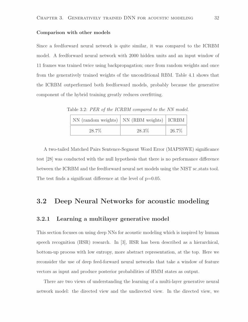
Comparison with other models
Since a feedforward neural network is quite similar, it was compared to the ICRBM
model. A feedforward neural network with 2000 hidden units and an input window of
11 frames was trained twice using backpropagation; once from random weights and once
from the generatively trained weights of the unconditional RBM. Table 4.1 shows that
the ICRBM outperformed both feedforward models, probably because the generative
component of the hybrid training greatly reduces overfitting.
Table 3.2: PER of the ICRBM compared to the NN model.
NN (random weights) NN (RBM weights) ICRBM
28.7% 28.3% 26.7%
A two-tailed Matched Pairs Sentence-Segment Word Error (MAPSSWE) significance
test [28] was conducted with the null hypothesis that there is no performance difference
between the ICRBM and the feedforward neural net models using the NIST sc stats tool.
The test finds a significant difference at the level of p=0.05.
3.2 Deep Neural Networks for acoustic modeling
3.2.1 Learning a multilayer generative model
This section focuses on using deep NNs for acoustic modeling which is inspired by human
speech recognition (HSR) research. In [3], HSR has been described as a hierarchical,
bottom-up process with low entropy, more abstract representation, at the top. Here we
reconsider the use of deep feed-forward neural networks that take a window of feature
vectors as input and produce posterior probabilities of HMM states as output.
There are two views of understanding the learning of a multi-layer generative neural
network model: the directed view and the undirected view. In the directed view, we
Chapter 3. Generatively trained DNN for acoustic modeling 33
fit a multilayer generative model that has infinitely many layers of latent variables, but
uses weight sharing among the higher layers to keep the number of parameters under
control [71]. This chapter focuses on the undirected, “energy-based” view, which is
in line with the discussion in section 3.1. In the undirected view, we fit a Restricted
Boltzmann Machine (RBM) to speech data, and then we treat the activities of the latent
variables as data for the next layer and fit an RBM again to these new “data”. This can
be repeated as many times as we like to learn as many layers of latent variables as we
desire.
Naturally, many of the high-level features learned by the generative model may be
irrelevant for making the required discriminations, even though they are important for
explaining the input data. However, this is a price worth paying if computation is cheap
and some of the high-level features are very good for discriminating between the classes
of interest.
The main novelty of the work presented in the remaining sections has been to show
that we can achieve consistently better phone recognition performance by “pre-training”
a multi-layer neural network, one layer at a time, as a generative model of the window of
speech coefficients. This pre-training makes it easier to optimize deep neural networks
that have many layers of hidden units and it also allows many more parameters to be
used before overfitting occurs. The generative pre-training creates many layers of feature
detectors that become progressively more complex. A subsequent phase of discriminative
fine-tuning, using the standard backpropagation algorithm, then adjusts the features in
every layer to make them more useful for discrimination.
Our approach makes two major assumptions about the nature of the relationship
between the input data, which in this case is a window of speech coefficients, and the
labels, which are HMM states produced by a forced alignment using a pre-existing ASR
model. First, we assume that the discrimination we want to perform is more directly
related to the underlying causes of the data than to the individual elements of the data
Chapter 3. Generatively trained DNN for acoustic modeling 34
itself. Second, we assume that a good feature-vector representation of the underlying
causes can be recovered from the input data by modeling its higher-order statistical
structure.
3.2.2 Using DNNs for phone recognition
As in the previous section, we use a context window of n successive frames of speech
coefficients to set the states of the visible units of the lowest RBM. Once it has been pre-
trained as a generative model, the resulting network is discriminatively trained to output
a probability distribution over the possible labels of the central frame. To generate phone
sequences, the sequence of predicted probability distributions over the possible labels for
each frame is fed into a standard Viterbi decoder.
Strictly speaking, since the HMM implements a prior over states, we should divide
out the prior from the posterior distribution over HMM states produced by the DNN,
although for the TIMIT task it made no difference.
3.2.3 Experiments
For all experiments conducted in this thesis, we fixed the parameters for the Viterbi
decoder. Specifically, we used a zero word-insertion probability and a language-model
scaling factor of 1.0.
All networks were pre-trained with a fixed recipe using stochastic gradient decent with
a mini-batch size of 128 training cases. For Gaussian-binary RBMs, we ran 225 epochs
with a fixed learning rate of 0.002 while for binary-binary RBMs we used 75 epochs with
a learning rate of 0.02. The learning rate is applied to the average gradient over each
mini-batch.
The theory used to justify the pre-training algorithm assumes that when the states of
the visible units are reconstructed from the inferred binary activities in the first hidden
layer, they are reconstructed stochastically. To reduce noise in the learning, we actually
Chapter 3. Generatively trained DNN for acoustic modeling 35
1 2 3 4 5 6 7 820
20.5
21
21.5
22
22.5
23
23.5
24
24.5
Number of layers
Phon
e er
ror r
ate
(PER
)
hid−1024−dev
hid−2048−dev
hid−3072−dev
hid−512−dev
Figure 3.2: Phone error rate on the development set as a function of the number of layers
and size of each layer, using 11 input frames.
reconstructed them deterministically and used the real values (see [43] for more details).
For fine-tuning, we used stochastic gradient descent with a mini-batch size 128 train-
ing cases. The learning rate started at 0.1. At the end of each epoch, if the recognition
error on the development set increased, the weights were returned to their values at
the beginning of the epoch and the learning rate was halved. This continued until the
learning rate fell below 0.001.
During both pre-training and fine-tuning, an L2 weight penalty, half of the sum
of squared weights, is used with small cost of 0.0002 and the learning was accelerated
by using a momentum of 0.9 (except for the first epoch of fine-tuning which did not use
momentum). [43] gives a detailed explanation of weight-cost and momentum and sensible
ways to set them. This training recipe has been used in all of the experiments conducted
in this thesis unless otherwise indicated.
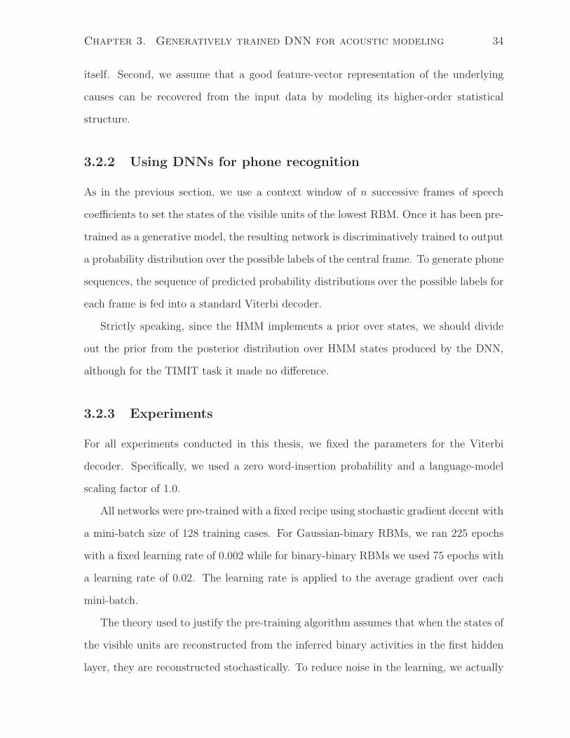
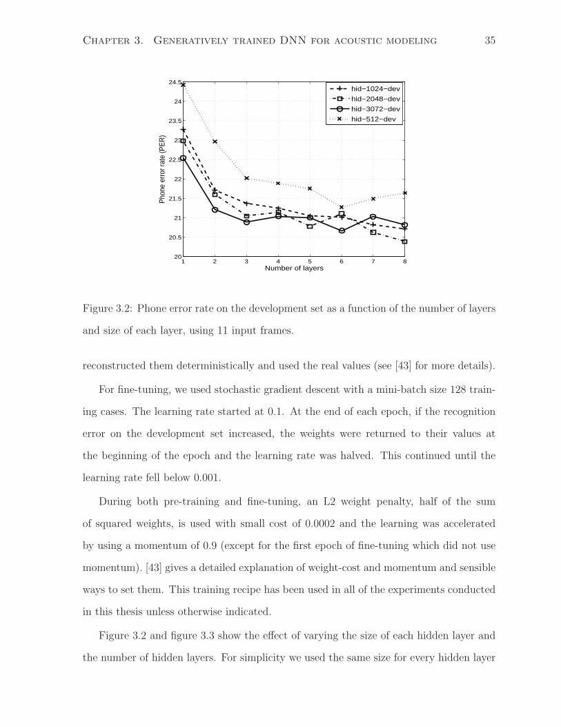
Figure 3.2 and figure 3.3 show the effect of varying the size of each hidden layer and
the number of hidden layers. For simplicity we used the same size for every hidden layer
Chapter 3. Generatively trained DNN for acoustic modeling 36
1 2 3 4 5 6 7 822
22.5
23
23.5
24
24.5
25
25.5
26
Number of layers
Phon
e er
ror r
ate
(PER
)
hid−1024−core
hid−2048−core
hid−3072−core
hid−512−core
Figure 3.3: Phone error rate on the core test set as a function of the number of layers
and size of each layer, using 11 input frames.
in the network. For these comparisons, the number of input frames was fixed at 11.
The main trend visible in figures 3.2, 3.3, 3.4, and 3.5 is that adding more hidden
layers gives better performance, even for non pre-trained deep networks, though the gain
diminishes as the number of layers increases. Using more hidden units per layer also
improves performance when the number of hidden layers is less than 4, but with more
hidden layers the number of units has little effect provided it is at least 1024. The
advantage of using a deep architecture is clear if we consider the best way to use a total
of 2048 hidden units: It is better to use two layers of 1024 or four layers of 512 than one
layer of 2048.
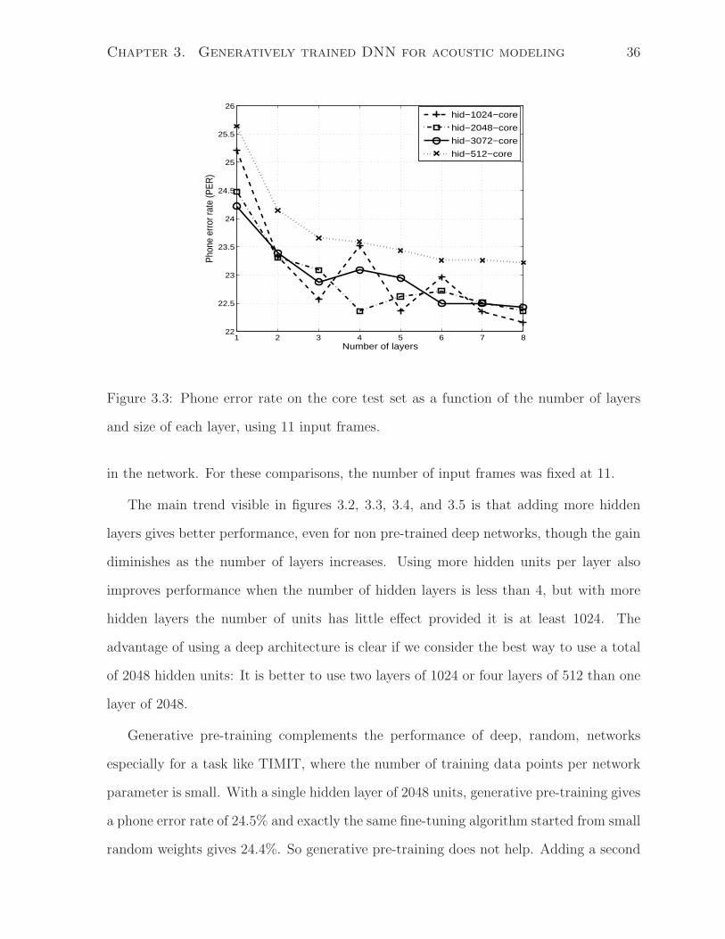
Generative pre-training complements the performance of deep, random, networks
especially for a task like TIMIT, where the number of training data points per network
parameter is small. With a single hidden layer of 2048 units, generative pre-training gives
a phone error rate of 24.5% and exactly the same fine-tuning algorithm started from small
random weights gives 24.4%. So generative pre-training does not help. Adding a second
Chapter 3. Generatively trained DNN for acoustic modeling 37
hidden layer causes a larger proportional increase in the number of trainable parameters
than adding a third hidden layer because the input and output layers are much smaller
than the hidden layers and because adjacent hidden layers are fully connected. This large
increase in capacity makes the model far more flexible, but it also makes it overfit far
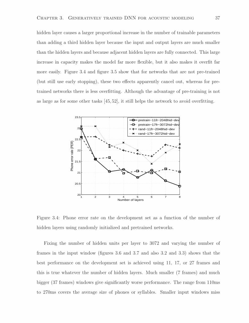
more easily. Figure 3.4 and figure 3.5 show that for networks that are not pre-trained
(but still use early stopping), these two effects apparently cancel out, whereas for pre-
trained networks there is less overfitting. Although the advantage of pre-training is not
as large as for some other tasks [45, 52], it still helps the network to avoid overfitting.
1 2 3 4 5 6 7 820
20.5
21
21.5
22
22.5
23
23.5
Number of layers
Phon
e er
ror r
ate
(PER
)
pretrain−11fr−2048hid−dev
pretrain−17fr−3072hid−dev
rand−11fr−2048hid−dev
rand−17fr−3072hid−dev
Figure 3.4: Phone error rate on the development set as a function of the number of
hidden layers using randomly initialized and pretrained networks.
Fixing the number of hidden units per layer to 3072 and varying the number of
frames in the input window (figures 3.6 and 3.7 and also 3.2 and 3.3) shows that the
best performance on the development set is achieved using 11, 17, or 27 frames and
this is true whatever the number of hidden layers. Much smaller (7 frames) and much
bigger (37 frames) windows give significantly worse performance. The range from 110ms
to 270ms covers the average size of phones or syllables. Smaller input windows miss
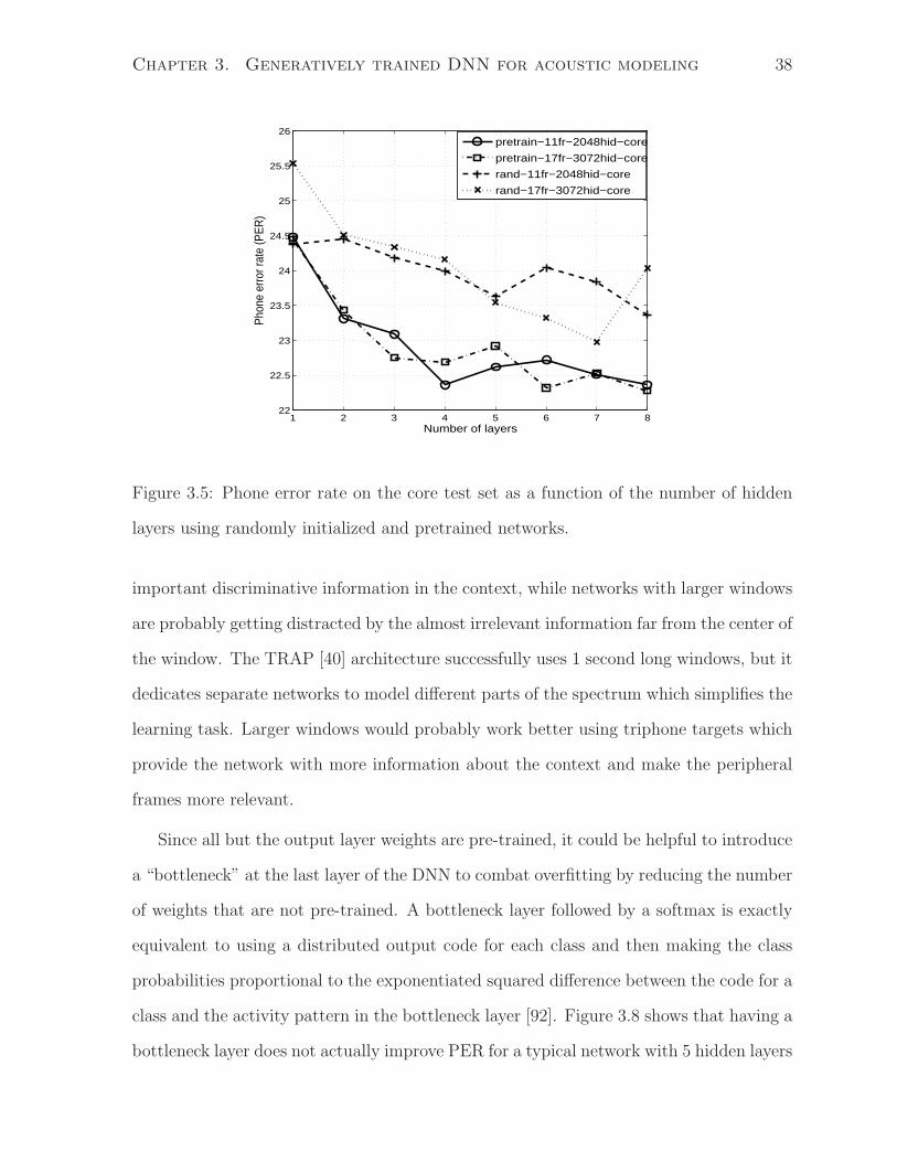
Chapter 3. Generatively trained DNN for acoustic modeling 38
1 2 3 4 5 6 7 822
22.5
23
23.5
24
24.5
25
25.5
26
Number of layers
Phon
e er
ror r
ate
(PER
)
pretrain−11fr−2048hid−core
pretrain−17fr−3072hid−core
rand−11fr−2048hid−core
rand−17fr−3072hid−core
Figure 3.5: Phone error rate on the core test set as a function of the number of hidden
layers using randomly initialized and pretrained networks.
important discriminative information in the context, while networks with larger windows
are probably getting distracted by the almost irrelevant information far from the center of
the window. The TRAP [40] architecture successfully uses 1 second long windows, but it
dedicates separate networks to model different parts of the spectrum which simplifies the
learning task. Larger windows would probably work better using triphone targets which
provide the network with more information about the context and make the peripheral
frames more relevant.
Since all but the output layer weights are pre-trained, it could be helpful to introduce
a “bottleneck” at the last layer of the DNN to combat overfitting by reducing the number
of weights that are not pre-trained. A bottleneck layer followed by a softmax is exactly
equivalent to using a distributed output code for each class and then making the class
probabilities proportional to the exponentiated squared difference between the code for a
class and the activity pattern in the bottleneck layer [92]. Figure 3.8 shows that having a
bottleneck layer does not actually improve PER for a typical network with 5 hidden layers
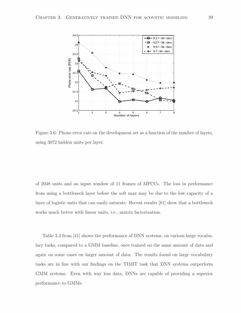
Chapter 3. Generatively trained DNN for acoustic modeling 39
1 2 3 4 5 6 7 820.5
21
21.5
22
22.5
23
23.5
24
24.5
Number of layers
Phon
e er
ror r
ate
(PER
)
fr17−3k−dev
fr27−3k−dev
fr37−3k−dev
fr7−3k−dev
Figure 3.6: Phone error rate on the development set as a function of the number of layers,
using 3072 hidden units per layer.
of 2048 units and an input window of 11 frames of MFCCs. The loss in performance
from using a bottleneck layer before the soft max may be due to the low capacity of a
layer of logistic units that can easily saturate. Recent results [81] show that a bottleneck
works much better with linear units, i.e., matrix factorization.
Table 3.3 from [41] shows the performance of DNN systems, on various large vocabu-
lary tasks, compared to a GMM baseline, once trained on the same amount of data and
again on some cases on larger amount of data. The results found on large vocabulary
tasks are in line with our findings on the TIMIT task that DNN systems outperform
GMM systems. Even with way less data, DNNs are capable of providing a superior
performance to GMMs.
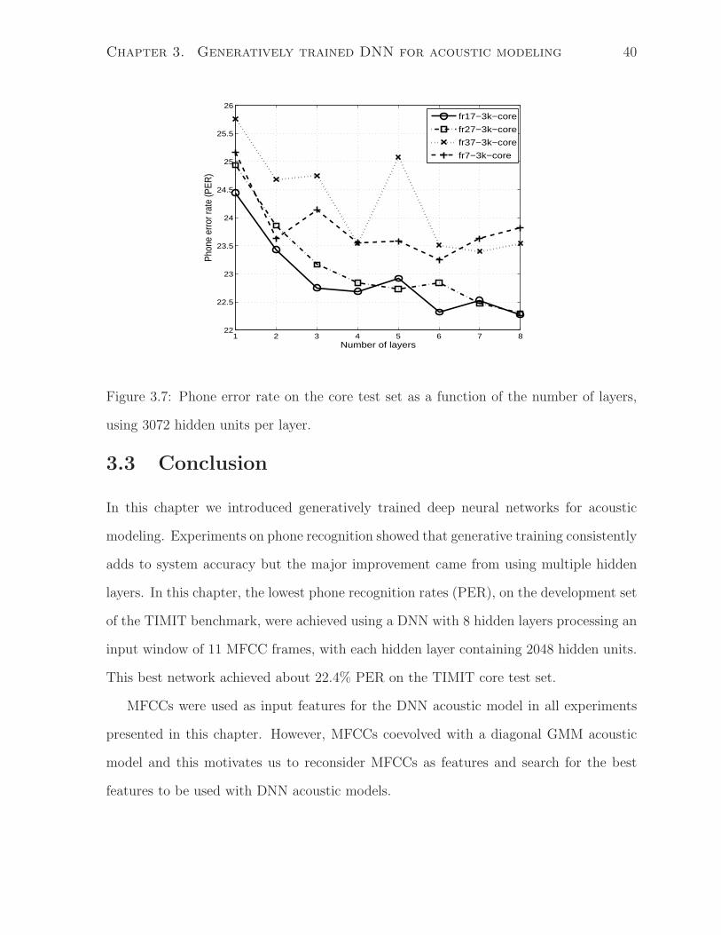
Chapter 3. Generatively trained DNN for acoustic modeling 40
1 2 3 4 5 6 7 822
22.5
23
23.5
24
24.5
25
25.5
26
Number of layers
Phon
e er
ror r
ate
(PER
)
fr17−3k−core
fr27−3k−core
fr37−3k−core
fr7−3k−core
Figure 3.7: Phone error rate on the core test set as a function of the number of layers,
using 3072 hidden units per layer.
3.3 Conclusion
In this chapter we introduced generatively trained deep neural networks for acoustic
modeling. Experiments on phone recognition showed that generative training consistently
adds to system accuracy but the major improvement came from using multiple hidden
layers. In this chapter, the lowest phone recognition rates (PER), on the development set
of the TIMIT benchmark, were achieved using a DNN with 8 hidden layers processing an
input window of 11 MFCC frames, with each hidden layer containing 2048 hidden units.
This best network achieved about 22.4% PER on the TIMIT core test set.
MFCCs were used as input features for the DNN acoustic model in all experiments
presented in this chapter. However, MFCCs coevolved with a diagonal GMM acoustic
model and this motivates us to reconsider MFCCs as features and search for the best
features to be used with DNN acoustic models.
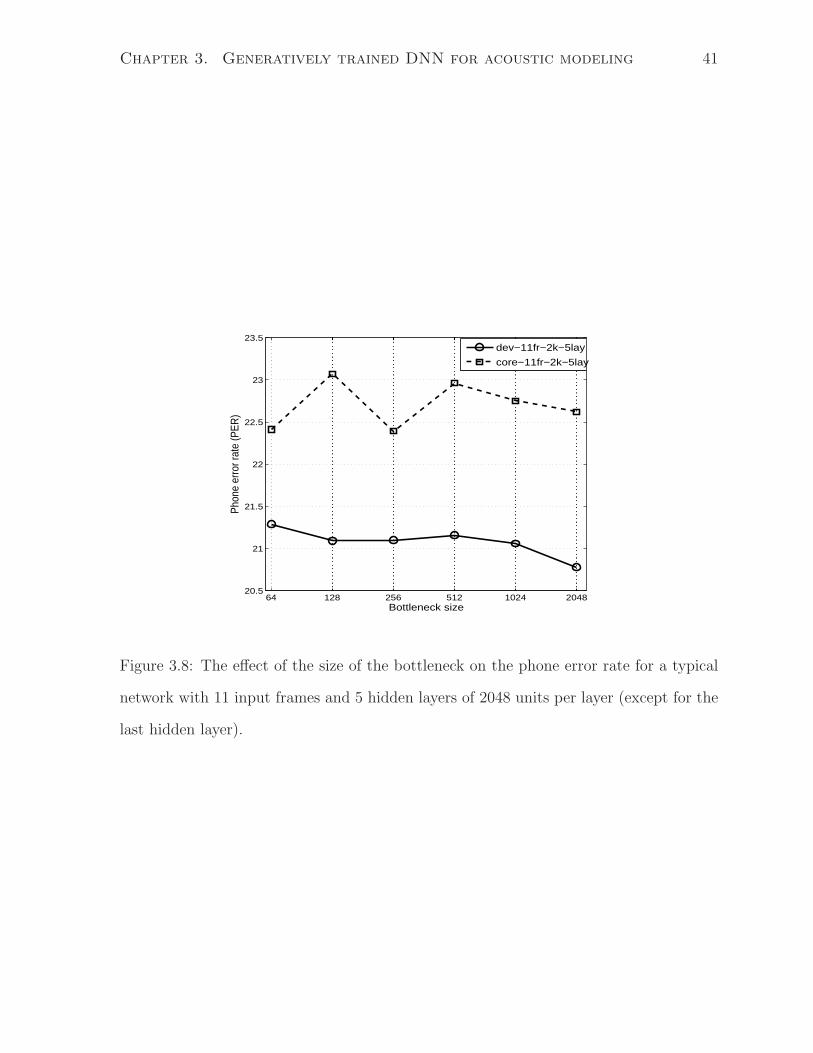
Chapter 3. Generatively trained DNN for acoustic modeling 41
64 128 256 512 1024 204820.5
21
21.5
22
22.5
23
23.5
Bottleneck size
Phon
e er
ror r
ate
(PER
)
dev−11fr−2k−5lay
core−11fr−2k−5lay
Figure 3.8: The effect of the size of the bottleneck on the phone error rate for a typical
network with 11 input frames and 5 hidden layers of 2048 units per layer (except for the
last hidden layer).
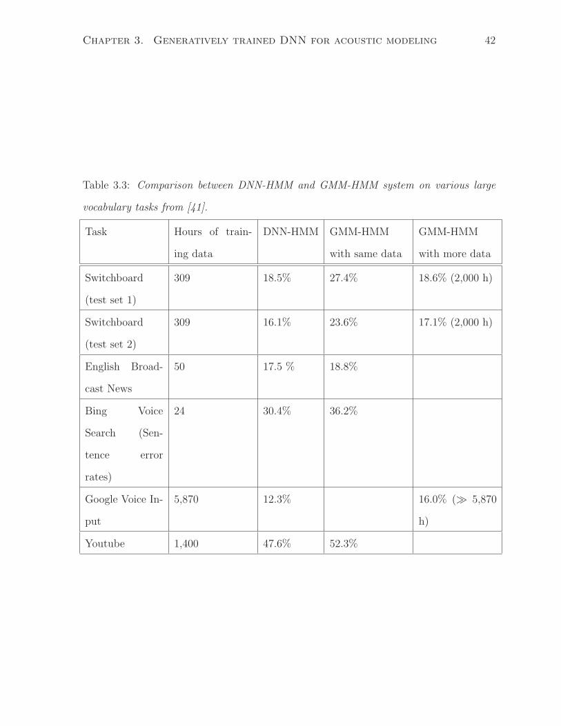
Chapter 3. Generatively trained DNN for acoustic modeling 42
Table 3.3: Comparison between DNN-HMM and GMM-HMM system on various large
vocabulary tasks from [41].
Task Hours of train-
ing data
DNN-HMM GMM-HMM
with same data
GMM-HMM
with more data
Switchboard
(test set 1)
309 18.5% 27.4% 18.6% (2,000 h)
Switchboard
(test set 2)
309 16.1% 23.6% 17.1% (2,000 h)
English Broad-
cast News
50 17.5 % 18.8%
Bing Voice
Search (Sen-
tence error
rates)
24 30.4% 36.2%
Google Voice In-
put
5,870 12.3% 16.0% (≫ 5,870
h)
Youtube 1,400 47.6% 52.3%
Chapter 4
Which features to use in a DNN
acoustic model
Speech data contain huge amounts of information, including aspects of the signal related
to the words spoken, the speaker’s emotional state, the dialect and identity of the speaker,
the language used, the physical location of the speech event, and the recording channel.
A key aim of the ASR feature extraction process is to ignore information in the input
signal that is not relevant to the spoken content, emphasizing elements that contribute
to detection of phonetic differences.
There have been various proposals for features which can represent the perceptually
relevant aspects of the short-term speech spectrum, based on a variety of signal processing
techniques, or based directly on the speech waveform [46]. A number of these proposals
are motivated by the results of human speech recognition research [12, 38, 39]. By far,
MFCCs are the most widely used input features for the state-of-the-art ASR systems.
One reason for the widespread use of MFCCs in ASR systems is that MFCCs have
many characteristics that are well suited to the HMM-GMM systems (with diagonal
covariance Gaussians) that have dominated the field. In this thesis, given that we are
proposing DNNs as a replacement for GMMs, we also need to reconsider the choice of
43
Chapter 4. Which features to use in a DNN acoustic model 44
MFCCs as features. MFCCs coevolved with GMMs, and there is no a priori reason to
believe that MFCCs should be the best input representations for DNN acoustic models.
In the previous chapter, we used MFCCs as our input features to the DNN model,
achieving a very competitive phone recognition performance. In this chapter, we will
study the desired characteristics of input features for DNN acoustic modeling.
4.1 Mel Frequency Cepstral Coefficients (MFCCs)
Motivated by observations in human speech recognition, Mel Frequency Cepstral Coeffi-
cients (MFCCs) were developed more than three decades ago [12]. They demonstrated the
best recognition accuracy relative to various other acoustic features. This is attributed
to their good representation of the perceptually relevant aspects of the short-term speech
spectrum. Here, we discuss briefly the main steps for producing MFCCs and the moti-
vation behind each step.
The first step involves producing the short-term speech spectrum of an input speech
window, typically between 25 to 30ms of speech. Peaks in the speech spectrum are
referred to as “formants”.
Human speech recognition research showed that the critical bandwidths for the human
ear are non-uniformally spaced along the frequency axis. The mel scale, which is linear
in low frequencies and logarithmic in high frequencies, was found to be a good candidate
to represent this non-uniformity. The result is the use of more filters in low frequency
regions and fewer filters in high frequency regions. The output of each filter corresponds
to the total energy in frequencies that lie within the range of that filter.
Another design decision, also based on HSR research, is to take the logarithm of filter
output values rather than just use the output values themselves. This is motivated by
the fact that the human ear doesn’t respond linearly to the amplitude of the input signal.
The features derived up to this step are called “log mel-frequency spectral Coefficients”
Chapter 4. Which features to use in a DNN acoustic model 45
or “MFSC”.
MFSC features were found to be highly correlated, with only a few eigenvectors
being sufficient to represent most of the information in the signal. This finding suggested
an economical, compressed representation for the speech spectrum. The first few basis
vectors of the discrete cosine transform (DCT) were found to be good, data-independent,
approximations of the principal dimensions.
The resulting MFCC coefficients are therefore produced by taking the first few bases
of the discrete cosine transform (DCT) of the real logarithm of the short-term energy
spectrum expressed on a mel-frequency scale. So, starting from highly correlated outputs
of greatly overlapping filters, the DCT concentrates energy in the first few coefficients
and decorrelates them.
MFCCs possess two important characteristics that have made them an integral part
of the state-of-the-art HMM-GMM systems:
• For each frame, MFCC features are decorrelated, which is preferred when diagonal
covariance GMMs are used for modeling. Diagonal covariance GMMs use far fewer
parameters than full covariance ones, which makes them robust for estimation as
well as faster for decoding since there is no matrix inversion required to compute the
Gaussian likelihoods. Diagonal covariance GMMs could be used to model correlated
features, but many more Gaussian components would be needed.
• MFCC features are more compact than MFSC features because they are projections
on the first few DCT basis vectors only.
As we can see, the whole process was motivated by human speech recognition findings,
but then the very last step, i.e., the DCT transform, was mainly motivated by the
model used, i.e., diagonal covariance GMMs, and by computational efficiency reasons.
For DNN acoustic models, the covariance structure of the data is modelled implicitly,
without any explicit assumptions about the data distribution, so there is no advantage in
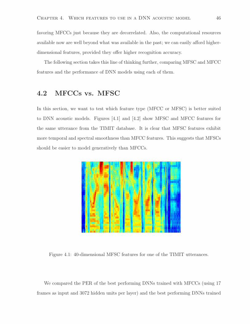
Chapter 4. Which features to use in a DNN acoustic model 46
favoring MFCCs just because they are decorrelated. Also, the computational resources
available now are well beyond what was available in the past; we can easily afford higher-
dimensional features, provided they offer higher recognition accuracy.
The following section takes this line of thinking further, comparing MFSC and MFCC
features and the performance of DNN models using each of them.
4.2 MFCCs vs. MFSC
In this section, we want to test which feature type (MFCC or MFSC) is better suited
to DNN acoustic models. Figures [4.1] and [4.2] show MFSC and MFCC features for
the same utterance from the TIMIT database. It is clear that MFSC features exhibit
more temporal and spectral smoothness than MFCC features. This suggests that MFSCs
should be easier to model generatively than MFCCs.
Figure 4.1: 40-dimensional MFSC features for one of the TIMIT utterances.
We compared the PER of the best performing DNNs trained with MFCCs (using 17
frames as input and 3072 hidden units per layer) and the best performing DNNs trained
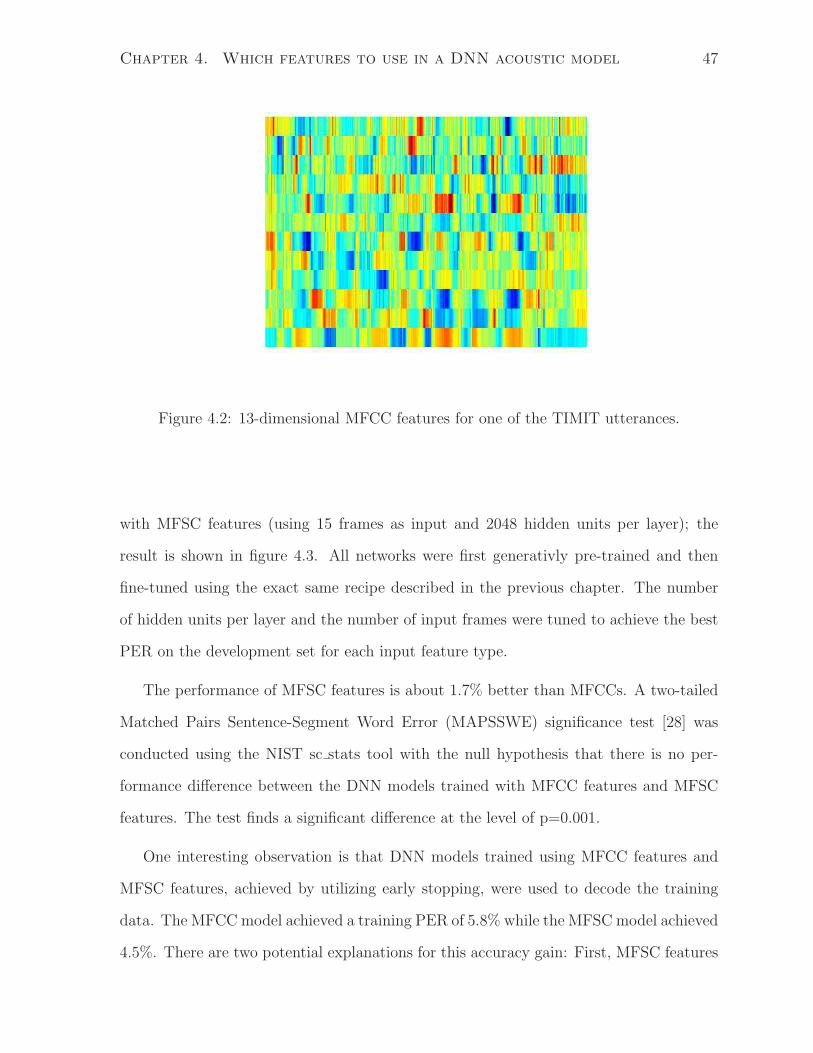
Chapter 4. Which features to use in a DNN acoustic model 47
Figure 4.2: 13-dimensional MFCC features for one of the TIMIT utterances.
with MFSC features (using 15 frames as input and 2048 hidden units per layer); the
result is shown in figure 4.3. All networks were first generativly pre-trained and then
fine-tuned using the exact same recipe described in the previous chapter. The number
of hidden units per layer and the number of input frames were tuned to achieve the best
PER on the development set for each input feature type.
The performance of MFSC features is about 1.7% better than MFCCs. A two-tailed
Matched Pairs Sentence-Segment Word Error (MAPSSWE) significance test [28] was
conducted using the NIST sc stats tool with the null hypothesis that there is no per-
formance difference between the DNN models trained with MFCC features and MFSC
features. The test finds a significant difference at the level of p=0.001.
One interesting observation is that DNN models trained using MFCC features and
MFSC features, achieved by utilizing early stopping, were used to decode the training
data. The MFCCmodel achieved a training PER of 5.8% while the MFSC model achieved
4.5%. There are two potential explanations for this accuracy gain: First, MFSC features
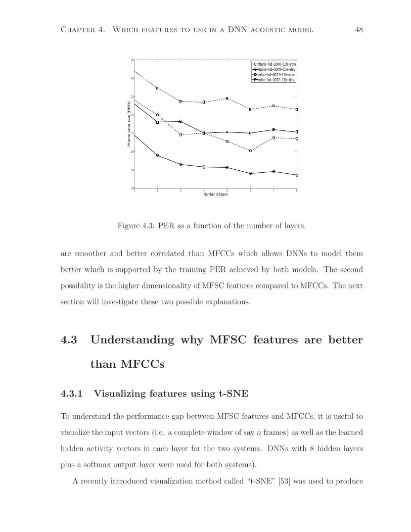
Chapter 4. Which features to use in a DNN acoustic model 48
1 2 3 4 5 6 7 818
19
20
21
22
23
24
25
Number of layers
Ph
on
e e
rro
r ra
te (
PE
R)
fbank−hid−2048−15fr−corefbank−hid−2048−15fr−devmfcc−hid−3072−17fr−coremfcc−hid−3072−17fr−dev
Figure 4.3: PER as a function of the number of layers.
are smoother and better correlated than MFCCs which allows DNNs to model them
better which is supported by the training PER achieved by both models. The second
possibility is the higher dimensionality of MFSC features compared to MFCCs. The next
section will investigate these two possible explanations.
4.3 Understanding why MFSC features are better
than MFCCs
4.3.1 Visualizing features using t-SNE
To understand the performance gap between MFSC features and MFCCs, it is useful to
visualize the input vectors (i.e. a complete window of say n frames) as well as the learned
hidden activity vectors in each layer for the two systems. DNNs with 8 hidden layers
plus a softmax output layer were used for both systems).
A recently introduced visualization method called “t-SNE” [53] was used to produce
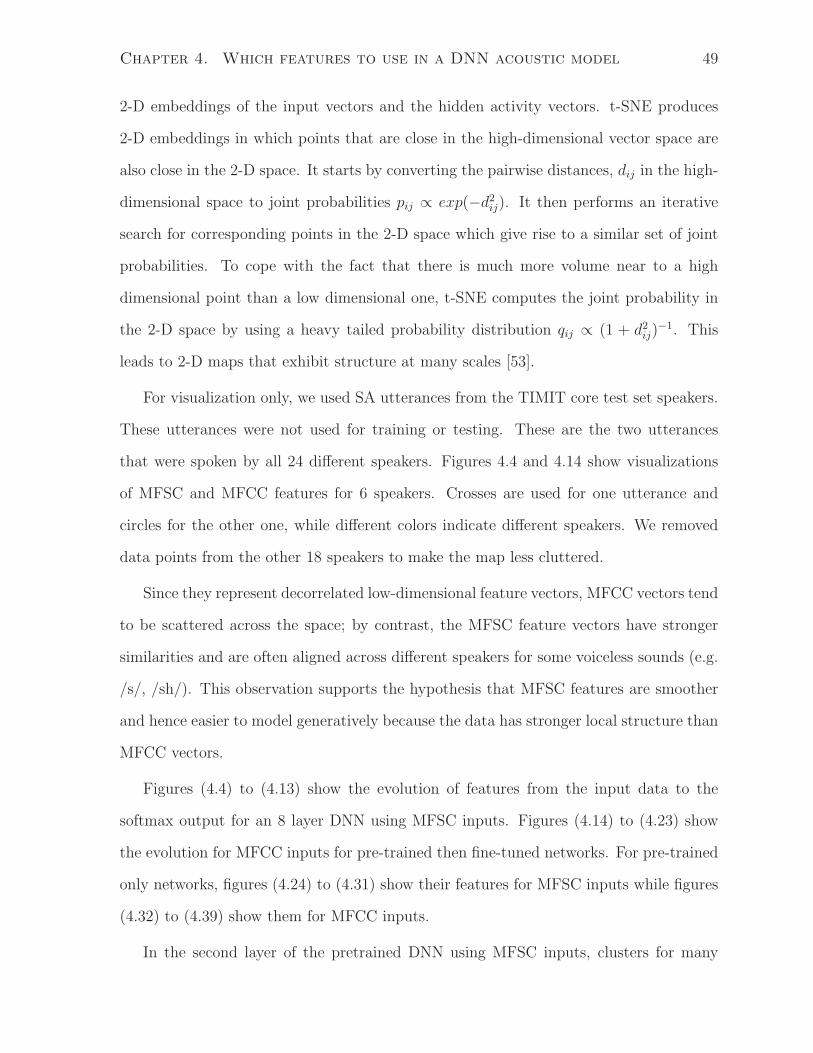
Chapter 4. Which features to use in a DNN acoustic model 49
2-D embeddings of the input vectors and the hidden activity vectors. t-SNE produces
2-D embeddings in which points that are close in the high-dimensional vector space are
also close in the 2-D space. It starts by converting the pairwise distances, dij in the high-
dimensional space to joint probabilities pij ∝ exp(−d2ij). It then performs an iterative
search for corresponding points in the 2-D space which give rise to a similar set of joint
probabilities. To cope with the fact that there is much more volume near to a high
dimensional point than a low dimensional one, t-SNE computes the joint probability in
the 2-D space by using a heavy tailed probability distribution qij ∝ (1 + d2ij)−1. This
leads to 2-D maps that exhibit structure at many scales [53].
For visualization only, we used SA utterances from the TIMIT core test set speakers.
These utterances were not used for training or testing. These are the two utterances
that were spoken by all 24 different speakers. Figures 4.4 and 4.14 show visualizations
of MFSC and MFCC features for 6 speakers. Crosses are used for one utterance and
circles for the other one, while different colors indicate different speakers. We removed
data points from the other 18 speakers to make the map less cluttered.
Since they represent decorrelated low-dimensional feature vectors, MFCC vectors tend
to be scattered across the space; by contrast, the MFSC feature vectors have stronger
similarities and are often aligned across different speakers for some voiceless sounds (e.g.
/s/, /sh/). This observation supports the hypothesis that MFSC features are smoother
and hence easier to model generatively because the data has stronger local structure than
MFCC vectors.
Figures (4.4) to (4.13) show the evolution of features from the input data to the
softmax output for an 8 layer DNN using MFSC inputs. Figures (4.14) to (4.23) show
the evolution for MFCC inputs for pre-trained then fine-tuned networks. For pre-trained
only networks, figures (4.24) to (4.31) show their features for MFSC inputs while figures
(4.32) to (4.39) show them for MFCC inputs.
In the second layer of the pretrained DNN using MFSC inputs, clusters for many
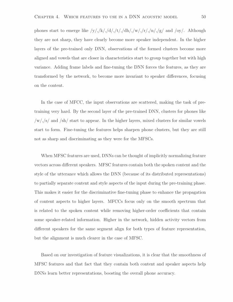
Chapter 4. Which features to use in a DNN acoustic model 50
phones start to emerge like /y/,/k/,/d/,/t/,/dh/,/w/,/r/,/n/,/g/ and /oy/. Although
they are not sharp, they have clearly become more speaker independent. In the higher
layers of the pre-trained only DNN, observations of the formed clusters become more
aligned and vowels that are closer in characteristics start to group together but with high
variance. Adding frame labels and fine-tuning the DNN forces the features, as they are
transformed by the network, to become more invariant to speaker differences, focusing
on the content.
In the case of MFCC, the input observations are scattered, making the task of pre-
training very hard. By the second layer of the pre-trained DNN, clusters for phones like
/w/,/s/ and /sh/ start to appear. In the higher layers, mixed clusters for similar vowels
start to form. Fine-tuning the features helps sharpen phone clusters, but they are still
not as sharp and discriminating as they were for the MFSCs.
When MFSC features are used, DNNs can be thought of implicitly normalizing feature
vectors across different speakers. MFSC features contain both the spoken content and the
style of the utterance which allows the DNN (because of its distributed representations)
to partially separate content and style aspects of the input during the pre-training phase.
This makes it easier for the discriminative fine-tuning phase to enhance the propagation
of content aspects to higher layers. MFCCs focus only on the smooth spectrum that
is related to the spoken content while removing higher-order coefficients that contain
some speaker-related information. Higher in the network, hidden activity vectors from
different speakers for the same segment align for both types of feature representation,
but the alignment is much clearer in the case of MFSC.
Based on our investigation of feature visualizations, it is clear that the smoothness of
MFSC features and that fact that they contain both content and speaker aspects help
DNNs learn better representations, boosting the overall phone accuracy.
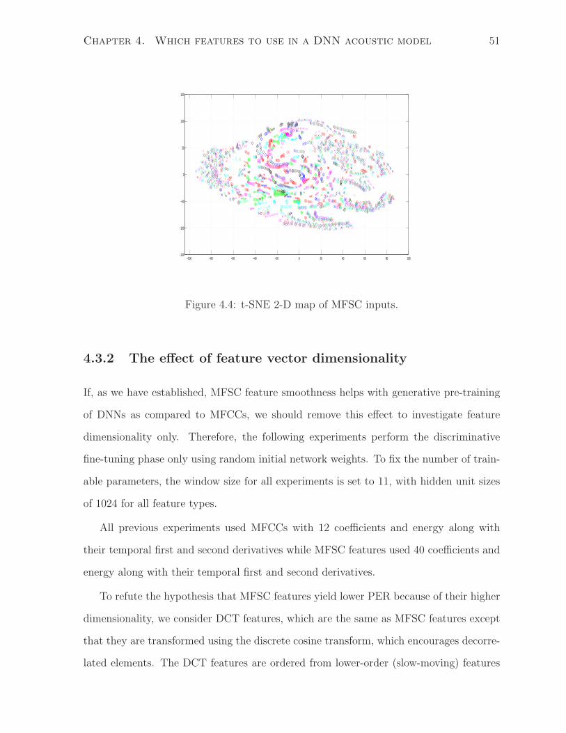
Chapter 4. Which features to use in a DNN acoustic model 51
−100 −80 −60 −40 −20 0 20 40 60 80 100−150
−100
−50
0
50
100
150
Figure 4.4: t-SNE 2-D map of MFSC inputs.
4.3.2 The effect of feature vector dimensionality
If, as we have established, MFSC feature smoothness helps with generative pre-training
of DNNs as compared to MFCCs, we should remove this effect to investigate feature
dimensionality only. Therefore, the following experiments perform the discriminative
fine-tuning phase only using random initial network weights. To fix the number of train-
able parameters, the window size for all experiments is set to 11, with hidden unit sizes
of 1024 for all feature types.
All previous experiments used MFCCs with 12 coefficients and energy along with
their temporal first and second derivatives while MFSC features used 40 coefficients and
energy along with their temporal first and second derivatives.
To refute the hypothesis that MFSC features yield lower PER because of their higher
dimensionality, we consider DCT features, which are the same as MFSC features except
that they are transformed using the discrete cosine transform, which encourages decorre-
lated elements. The DCT features are ordered from lower-order (slow-moving) features
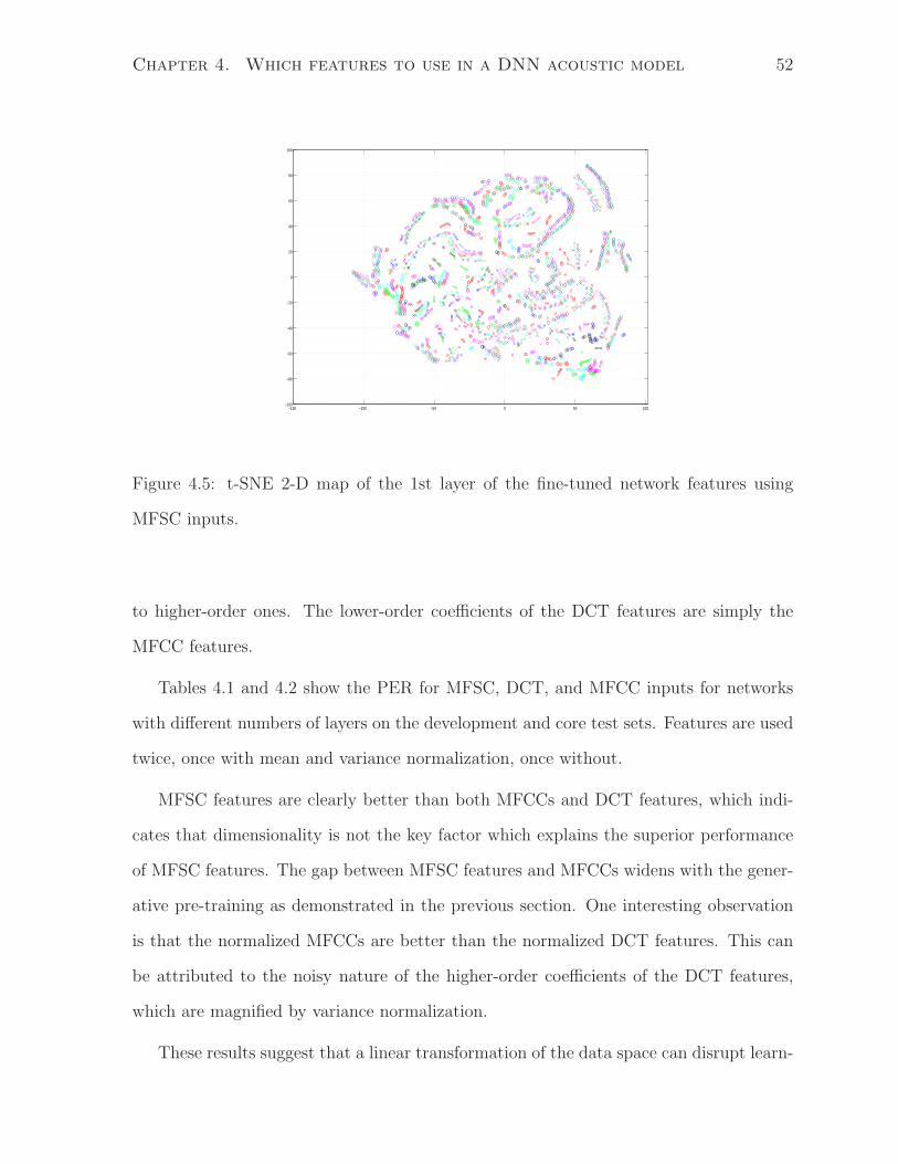
Chapter 4. Which features to use in a DNN acoustic model 52
−150 −100 −50 0 50 100−100
−80
−60
−40
−20
0
20
40
60
80
100
Figure 4.5: t-SNE 2-D map of the 1st layer of the fine-tuned network features using
MFSC inputs.
to higher-order ones. The lower-order coefficients of the DCT features are simply the
MFCC features.
Tables 4.1 and 4.2 show the PER for MFSC, DCT, and MFCC inputs for networks
with different numbers of layers on the development and core test sets. Features are used
twice, once with mean and variance normalization, once without.
MFSC features are clearly better than both MFCCs and DCT features, which indi-
cates that dimensionality is not the key factor which explains the superior performance
of MFSC features. The gap between MFSC features and MFCCs widens with the gener-
ative pre-training as demonstrated in the previous section. One interesting observation
is that the normalized MFCCs are better than the normalized DCT features. This can
be attributed to the noisy nature of the higher-order coefficients of the DCT features,
which are magnified by variance normalization.
These results suggest that a linear transformation of the data space can disrupt learn-
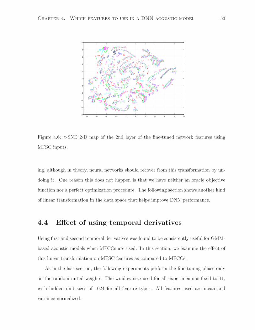
Chapter 4. Which features to use in a DNN acoustic model 53
−80 −60 −40 −20 0 20 40 60 80 100 120−100
−80
−60
−40
−20
0
20
40
60
80
100
Figure 4.6: t-SNE 2-D map of the 2nd layer of the fine-tuned network features using
MFSC inputs.
ing, although in theory, neural networks should recover from this transformation by un-
doing it. One reason this does not happen is that we have neither an oracle objective
function nor a perfect optimization procedure. The following section shows another kind
of linear transformation in the data space that helps improve DNN performance.
4.4 Effect of using temporal derivatives
Using first and second temporal derivatives was found to be consistently useful for GMM-
based acoustic models when MFCCs are used. In this section, we examine the effect of
this linear transformation on MFSC features as compared to MFCCs.
As in the last section, the following experiments perform the fine-tuning phase only
on the random initial weights. The window size used for all experiments is fixed to 11,
with hidden unit sizes of 1024 for all feature types. All features used are mean and
variance normalized.
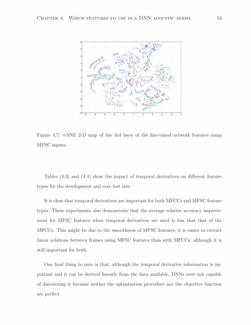
Chapter 4. Which features to use in a DNN acoustic model 54
−100 −80 −60 −40 −20 0 20 40 60 80 100−100
−80
−60
−40
−20
0
20
40
60
80
100
Figure 4.7: t-SNE 2-D map of the 3rd layer of the fine-tuned network features using
MFSC inputs.
Tables (4.3) and (4.4) show the impact of temporal derivatives on different feature
types for the development and core test sets.
It is clear that temporal derivatives are important for both MFCCs and MFSC feature
types. These experiments also demonstrate that the average relative accuracy improve-
ment for MFSC features when temporal derivatives are used is less that that of the
MFCCs. This might be due to the smoothness of MFSC features; it is easier to extract
linear relations between frames using MFSC features than with MFCCs, although it is
still important for both.
One final thing to note is that, although the temporal derivative information is im-
portant and it can be derived linearly from the data available, DNNs were not capable
of discovering it because neither the optimization procedure nor the objective function
are perfect.
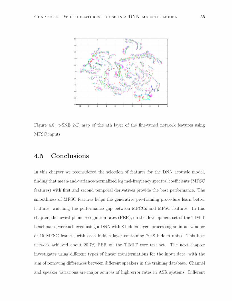
Chapter 4. Which features to use in a DNN acoustic model 55
−100 −80 −60 −40 −20 0 20 40 60 80 100−100
−80
−60
−40
−20
0
20
40
60
80
100
Figure 4.8: t-SNE 2-D map of the 4th layer of the fine-tuned network features using
MFSC inputs.
4.5 Conclusions
In this chapter we reconsidered the selection of features for the DNN acoustic model,
finding that mean-and-variance-normalized log mel-frequency spectral coefficients (MFSC
features) with first and second temporal derivatives provide the best performance. The
smoothness of MFSC features helps the generative pre-training procedure learn better
features, widening the performance gap between MFCCs and MFSC features. In this
chapter, the lowest phone recognition rates (PER), on the development set of the TIMIT
benchmark, were achieved using a DNN with 8 hidden layers processing an input window
of 15 MFSC frames, with each hidden layer containing 2048 hidden units. This best
network achieved about 20.7% PER on the TIMIT core test set. The next chapter
investigates using different types of linear transformations for the input data, with the
aim of removing differences between different speakers in the training database. Channel
and speaker variations are major sources of high error rates in ASR systems. Different
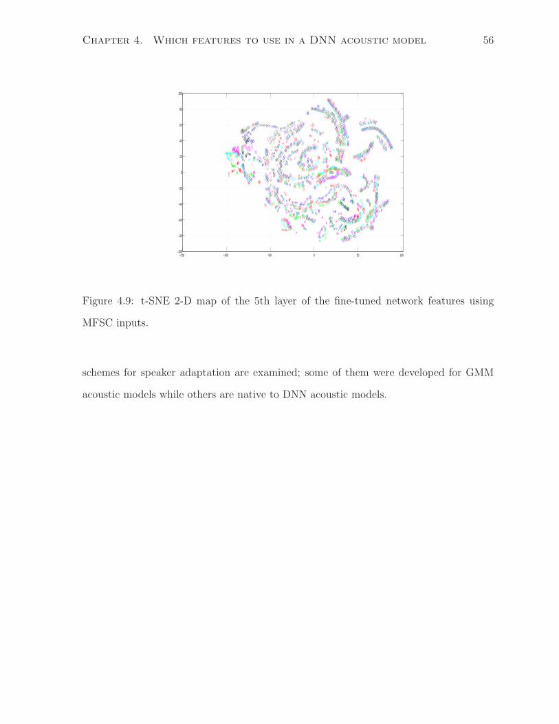
Chapter 4. Which features to use in a DNN acoustic model 56
−150 −100 −50 0 50 100−100
−80
−60
−40
−20
0
20
40
60
80
100
Figure 4.9: t-SNE 2-D map of the 5th layer of the fine-tuned network features using
MFSC inputs.
schemes for speaker adaptation are examined; some of them were developed for GMM
acoustic models while others are native to DNN acoustic models.
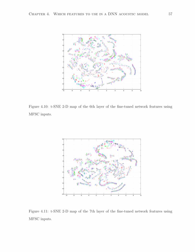
Chapter 4. Which features to use in a DNN acoustic model 57
−80 −60 −40 −20 0 20 40 60 80 100−100
−80
−60
−40
−20
0
20
40
60
80
100
Figure 4.10: t-SNE 2-D map of the 6th layer of the fine-tuned network features using
MFSC inputs.
−100 −80 −60 −40 −20 0 20 40 60 80 100−100
−80
−60
−40
−20
0
20
40
60
80
100
Figure 4.11: t-SNE 2-D map of the 7th layer of the fine-tuned network features using
MFSC inputs.
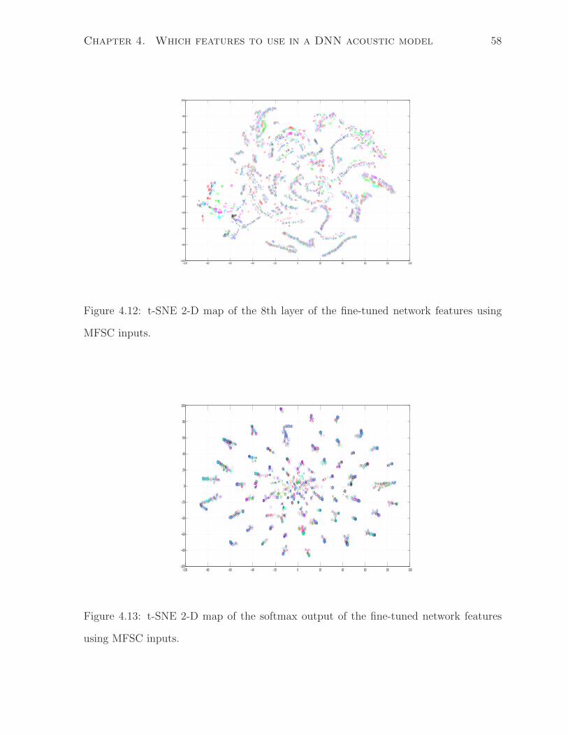
Chapter 4. Which features to use in a DNN acoustic model 58
−100 −80 −60 −40 −20 0 20 40 60 80 100−100
−80
−60
−40
−20
0
20
40
60
80
100
Figure 4.12: t-SNE 2-D map of the 8th layer of the fine-tuned network features using
MFSC inputs.
−100 −80 −60 −40 −20 0 20 40 60 80 100−100
−80
−60
−40
−20
0
20
40
60
80
100
Figure 4.13: t-SNE 2-D map of the softmax output of the fine-tuned network features
using MFSC inputs.
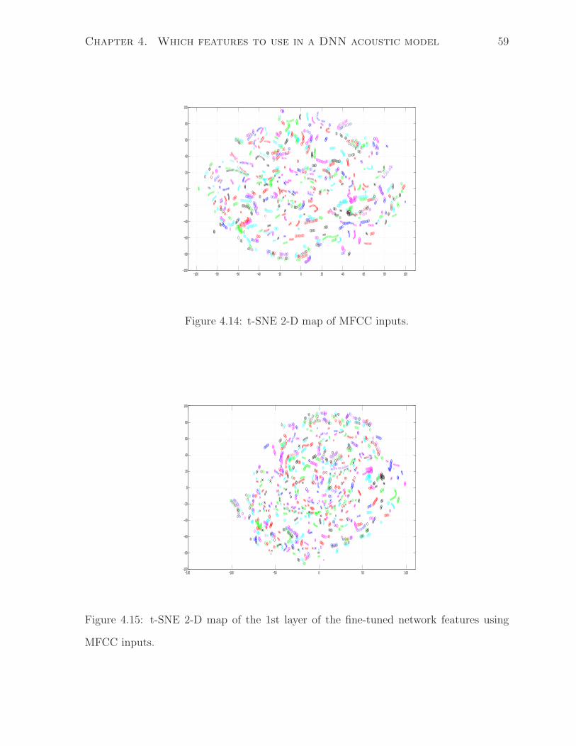
Chapter 4. Which features to use in a DNN acoustic model 59
−100 −80 −60 −40 −20 0 20 40 60 80 100−100
−80
−60
−40
−20
0
20
40
60
80
100
Figure 4.14: t-SNE 2-D map of MFCC inputs.
−150 −100 −50 0 50 100−100
−80
−60
−40
−20
0
20
40
60
80
100
Figure 4.15: t-SNE 2-D map of the 1st layer of the fine-tuned network features using
MFCC inputs.
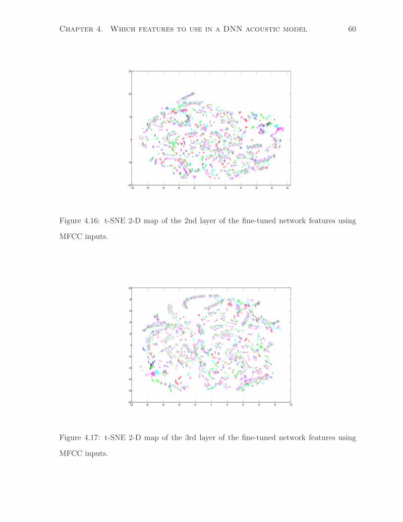
Chapter 4. Which features to use in a DNN acoustic model 60
−100 −80 −60 −40 −20 0 20 40 60 80 100−100
−50
0
50
100
150
Figure 4.16: t-SNE 2-D map of the 2nd layer of the fine-tuned network features using
MFCC inputs.
−100 −80 −60 −40 −20 0 20 40 60 80 100−100
−80
−60
−40
−20
0
20
40
60
80
100
Figure 4.17: t-SNE 2-D map of the 3rd layer of the fine-tuned network features using
MFCC inputs.
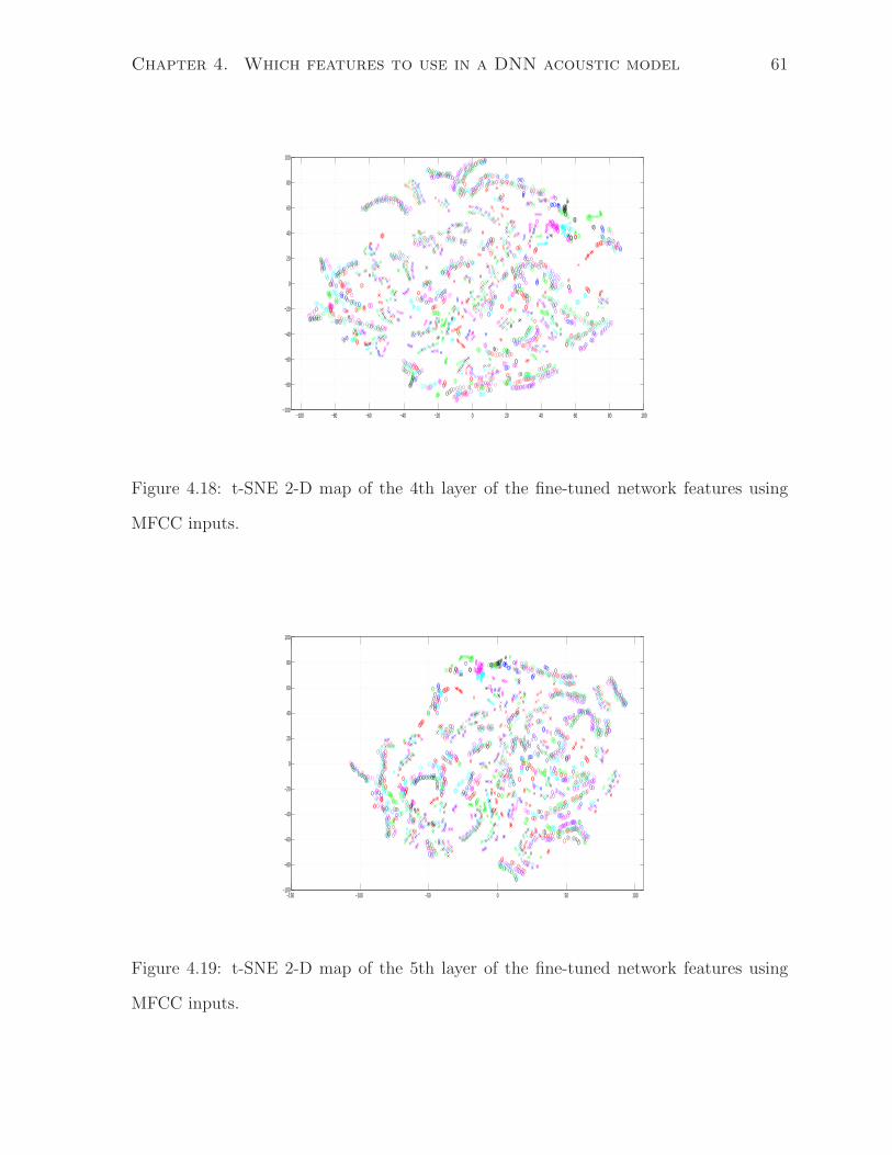
Chapter 4. Which features to use in a DNN acoustic model 61
−100 −80 −60 −40 −20 0 20 40 60 80 100−100
−80
−60
−40
−20
0
20
40
60
80
100
Figure 4.18: t-SNE 2-D map of the 4th layer of the fine-tuned network features using
MFCC inputs.
−150 −100 −50 0 50 100−100
−80
−60
−40
−20
0
20
40
60
80
100
Figure 4.19: t-SNE 2-D map of the 5th layer of the fine-tuned network features using
MFCC inputs.
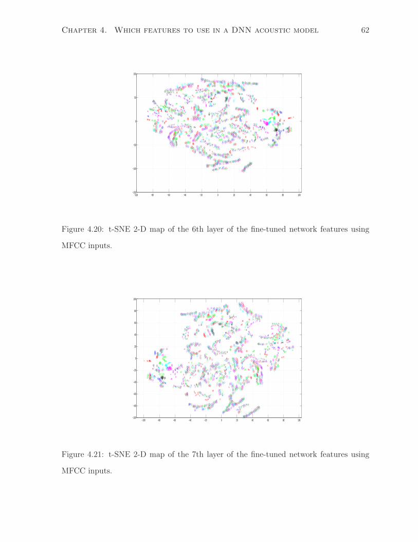
Chapter 4. Which features to use in a DNN acoustic model 62
−100 −80 −60 −40 −20 0 20 40 60 80 100−150
−100
−50
0
50
100
Figure 4.20: t-SNE 2-D map of the 6th layer of the fine-tuned network features using
MFCC inputs.
−100 −80 −60 −40 −20 0 20 40 60 80 100−100
−80
−60
−40
−20
0
20
40
60
80
100
Figure 4.21: t-SNE 2-D map of the 7th layer of the fine-tuned network features using
MFCC inputs.
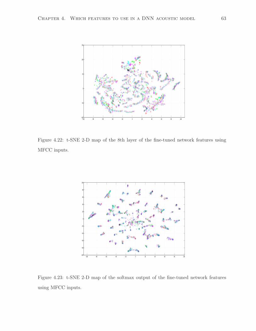
Chapter 4. Which features to use in a DNN acoustic model 63
−100 −80 −60 −40 −20 0 20 40 60 80 100−100
−50
0
50
100
150
Figure 4.22: t-SNE 2-D map of the 8th layer of the fine-tuned network features using
MFCC inputs.
−100 −80 −60 −40 −20 0 20 40 60 80 100−100
−80
−60
−40
−20
0
20
40
60
80
100
Figure 4.23: t-SNE 2-D map of the softmax output of the fine-tuned network features
using MFCC inputs.
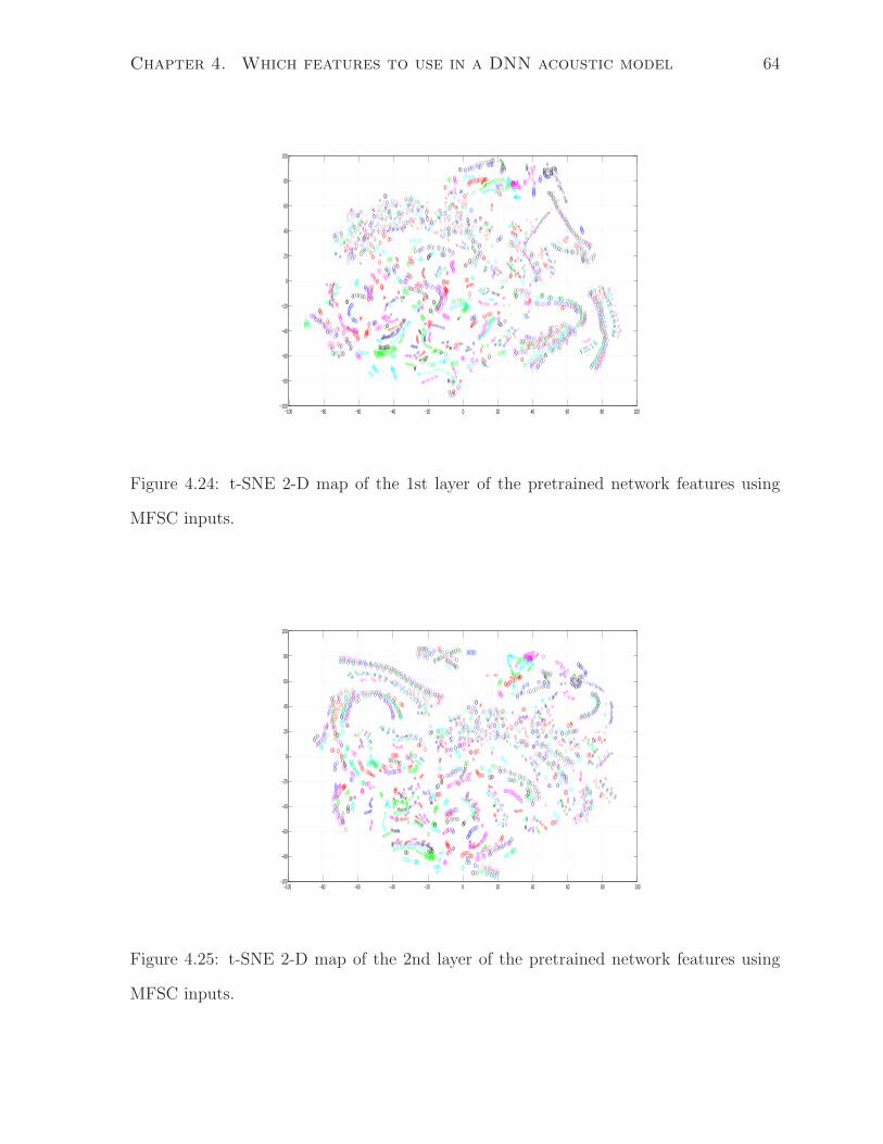
Chapter 4. Which features to use in a DNN acoustic model 64
−100 −80 −60 −40 −20 0 20 40 60 80 100−100
−80
−60
−40
−20
0
20
40
60
80
100
Figure 4.24: t-SNE 2-D map of the 1st layer of the pretrained network features using
MFSC inputs.
−100 −80 −60 −40 −20 0 20 40 60 80 100−100
−80
−60
−40
−20
0
20
40
60
80
100
Figure 4.25: t-SNE 2-D map of the 2nd layer of the pretrained network features using
MFSC inputs.
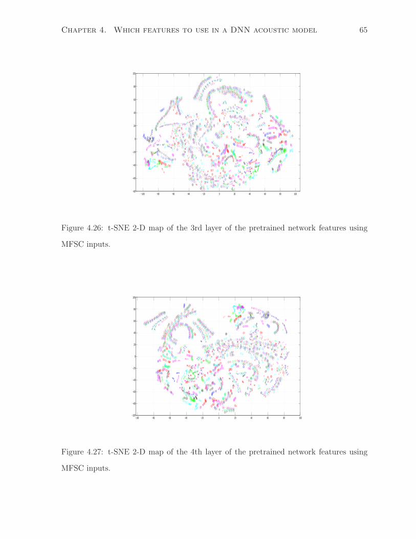
Chapter 4. Which features to use in a DNN acoustic model 65
−100 −80 −60 −40 −20 0 20 40 60 80 100−80
−60
−40
−20
0
20
40
60
80
100
Figure 4.26: t-SNE 2-D map of the 3rd layer of the pretrained network features using
MFSC inputs.
−100 −80 −60 −40 −20 0 20 40 60 80 100−100
−80
−60
−40
−20
0
20
40
60
80
100
Figure 4.27: t-SNE 2-D map of the 4th layer of the pretrained network features using
MFSC inputs.
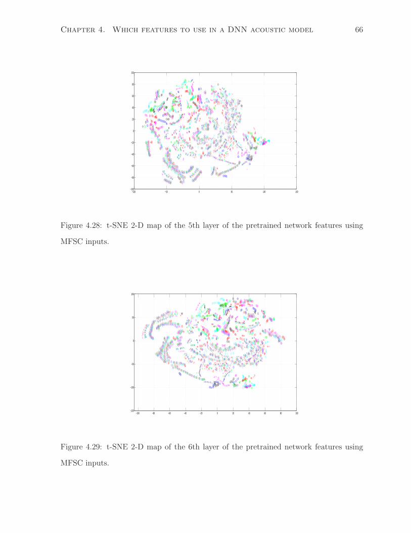
Chapter 4. Which features to use in a DNN acoustic model 66
−100 −50 0 50 100 150−100
−80
−60
−40
−20
0
20
40
60
80
100
Figure 4.28: t-SNE 2-D map of the 5th layer of the pretrained network features using
MFSC inputs.
−100 −80 −60 −40 −20 0 20 40 60 80 100−150
−100
−50
0
50
100
Figure 4.29: t-SNE 2-D map of the 6th layer of the pretrained network features using
MFSC inputs.
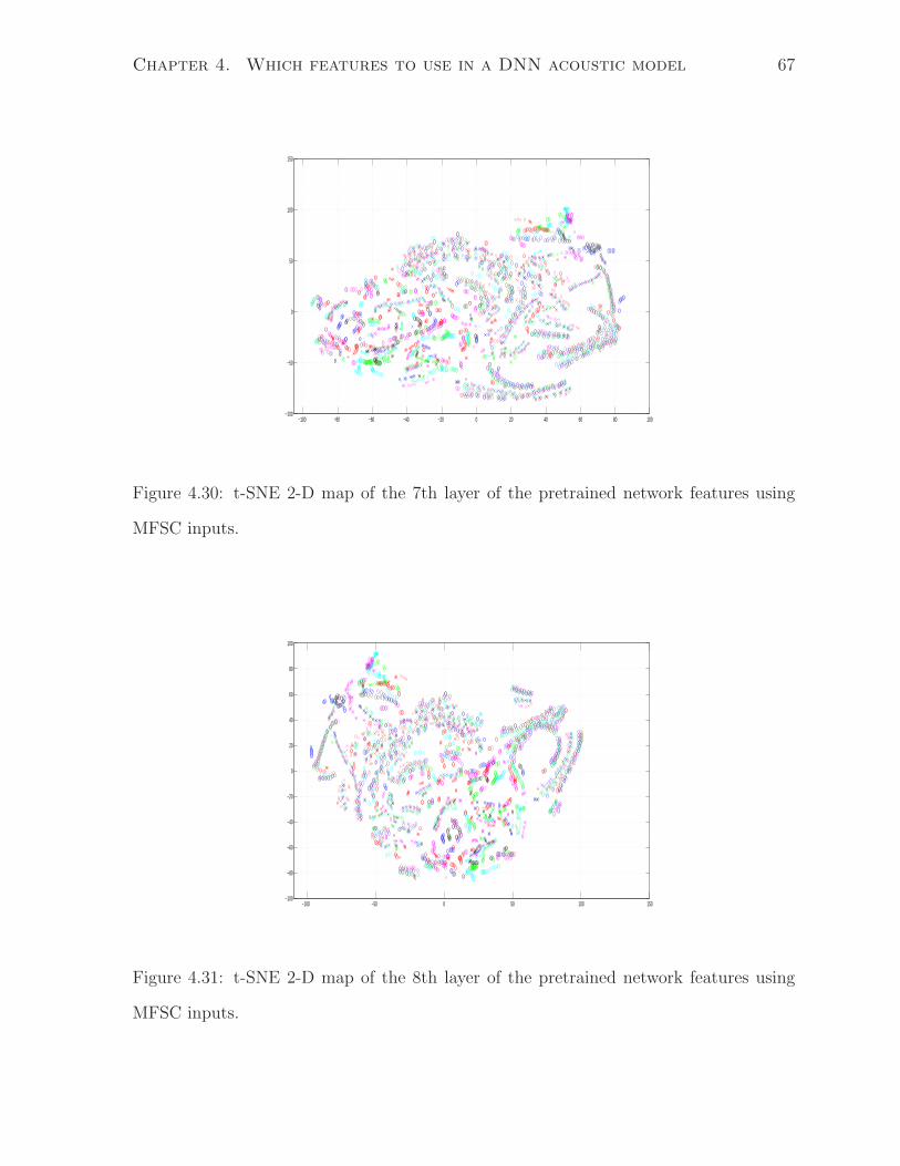
Chapter 4. Which features to use in a DNN acoustic model 67
−100 −80 −60 −40 −20 0 20 40 60 80 100−100
−50
0
50
100
150
Figure 4.30: t-SNE 2-D map of the 7th layer of the pretrained network features using
MFSC inputs.
−100 −50 0 50 100 150−100
−80
−60
−40
−20
0
20
40
60
80
100
Figure 4.31: t-SNE 2-D map of the 8th layer of the pretrained network features using
MFSC inputs.
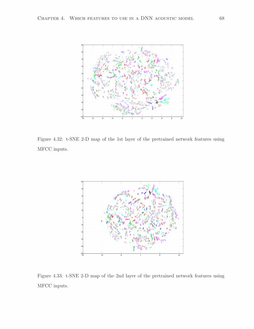
Chapter 4. Which features to use in a DNN acoustic model 68
−100 −80 −60 −40 −20 0 20 40 60 80 100−100
−80
−60
−40
−20
0
20
40
60
80
100
Figure 4.32: t-SNE 2-D map of the 1st layer of the pretrained network features using
MFCC inputs.
−150 −100 −50 0 50 100−100
−80
−60
−40
−20
0
20
40
60
80
100
Figure 4.33: t-SNE 2-D map of the 2nd layer of the pretrained network features using
MFCC inputs.
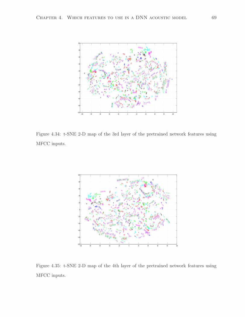
Chapter 4. Which features to use in a DNN acoustic model 69
−100 −80 −60 −40 −20 0 20 40 60 80 100−100
−80
−60
−40
−20
0
20
40
60
80
100
Figure 4.34: t-SNE 2-D map of the 3rd layer of the pretrained network features using
MFCC inputs.
−100 −80 −60 −40 −20 0 20 40 60 80 100−100
−80
−60
−40
−20
0
20
40
60
80
100
Figure 4.35: t-SNE 2-D map of the 4th layer of the pretrained network features using
MFCC inputs.
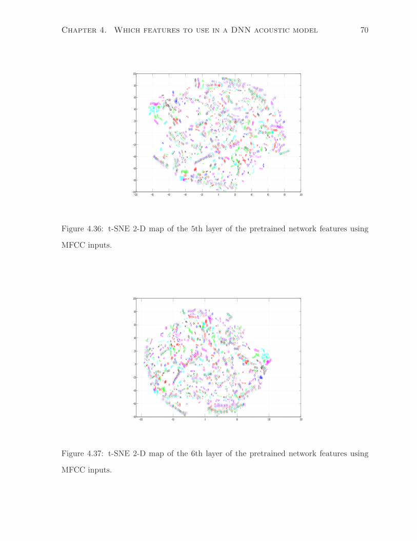
Chapter 4. Which features to use in a DNN acoustic model 70
−100 −80 −60 −40 −20 0 20 40 60 80 100−100
−80
−60
−40
−20
0
20
40
60
80
100
Figure 4.36: t-SNE 2-D map of the 5th layer of the pretrained network features using
MFCC inputs.
−100 −50 0 50 100 150−80
−60
−40
−20
0
20
40
60
80
100
Figure 4.37: t-SNE 2-D map of the 6th layer of the pretrained network features using
MFCC inputs.
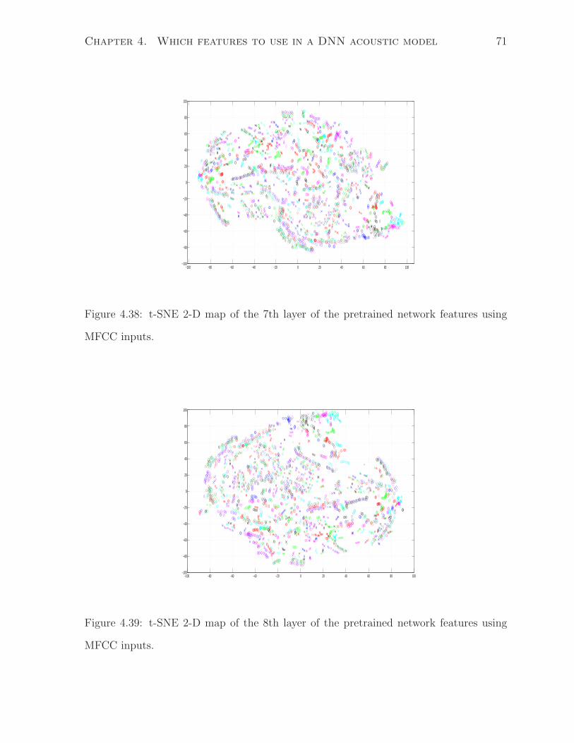
Chapter 4. Which features to use in a DNN acoustic model 71
−100 −80 −60 −40 −20 0 20 40 60 80 100−100
−80
−60
−40
−20
0
20
40
60
80
100
Figure 4.38: t-SNE 2-D map of the 7th layer of the pretrained network features using
MFCC inputs.
−100 −80 −60 −40 −20 0 20 40 60 80 100−100
−80
−60
−40
−20
0
20
40
60
80
100
Figure 4.39: t-SNE 2-D map of the 8th layer of the pretrained network features using
MFCC inputs.

Chapter 4. Which features to use in a DNN acoustic model 72
Table 4.1: The PER deep nets using various features on the development set
Feature Dim 1lay 2lay 3lay 4lay
MFSC 123 23.33% 21.45% 21.06% 21.5%
MFSC+norm 123 22.25% 21.3% 21.31% 21.46%
DCT 123 25.55% 23.67% 23.62% 23.23%
DCT+norm 123 24.48% 22.9% 22.58% 23.31%
MFCC 39 25.95% 24.06% 23.99% 23.98%
MFCC+norm 39 23.2% 21.87% 22.02% 21.99%
Table 4.2: The PER deep nets using various features on the core test set
Feature Dim 1lay 2lay 3lay 4lay
MFSC 123 24.9% 23.58% 22.62% 23.06%
MFSC+norm 123 23.86% 22.58% 22.88% 22.83%
DCT 123 27.22% 25.42% 25.75% 25.58%
DCT+norm 123 26.13% 24.04% 24.49% 25.27%
MFCC 39 27.15% 26.09% 26.2% 25.56%
MFCC+norm 39 24.72% 23.67% 23.62% 23.66%
Table 4.3: Effect of temporal derivatives on the PER of the development set
Feature Dim 1lay 2lay 3lay 4lay
MFSC 41 23.14% 22.31% 22.25% 22.08%
MFSC+D 82 22.53% 21.56% 20.96% 21.46%
MFSC+D+DD 123 22.25% 21.3% 21.31% 21.46%
MFCC 13 24.19% 23% 23.11% 23.16%
MFCC+D 26 23.32% 22.12% 22.17% 22.4%
MFCC+D+DD 39 23.2% 21.87% 22.02% 21.99%
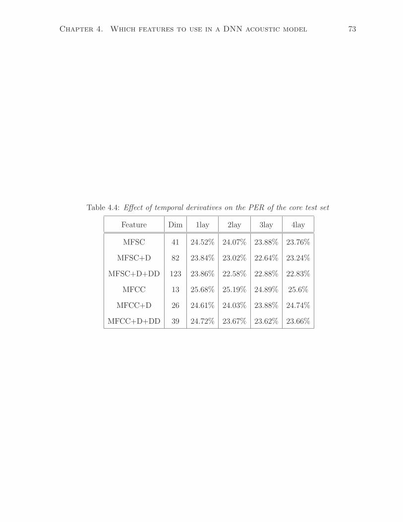
Chapter 4. Which features to use in a DNN acoustic model 73
Table 4.4: Effect of temporal derivatives on the PER of the core test set
Feature Dim 1lay 2lay 3lay 4lay
MFSC 41 24.52% 24.07% 23.88% 23.76%
MFSC+D 82 23.84% 23.02% 22.64% 23.24%
MFSC+D+DD 123 23.86% 22.58% 22.88% 22.83%
MFCC 13 25.68% 25.19% 24.89% 25.6%
MFCC+D 26 24.61% 24.03% 23.88% 24.74%
MFCC+D+DD 39 24.72% 23.67% 23.62% 23.66%
Chapter 5
Speaker adaptive training in DNN
acoustic models
Humans have an amazing ability to recognize and adapt to a large range of speech,
speaker, channel, and environmental conditions which current ASR systems fail dramati-
cally to do. Accurate ASR output for such diverse conditions has been selected as one of
the “Grand Challenges” facing ASR research by a team of ASR leading researchers [7].
Many “adaptation” techniques have been developed to deal with background and
speaker variability [2, 21, 26]. One way to think about adaptation, that was found suc-
cessful, is to transform the trained model (the training distribution) to comply with the
testing conditions (the testing distribution) so that the likelihood of the test data is max-
imized under the new model. This type of adaptation is performed during the testing
phase.
A different kind of adaptation is to eliminate differences in the training data that do
not contribute towards better system accuracy, e.g., normalizing inter-speaker variabil-
ity in the training data while keeping intra-speaker variability by mapping all training
speakers to a similar canonical speaker. Here we focus on this second type of adaptation,
which takes place during model training. It focuses only on speaker adaptation but the
74
Chapter 5. Speaker adaptive training in DNN acoustic models 75
work presented is applicable to background and channel adaptation as well.
The DNN acoustic model proposed in previous chapters does not include any special
procedure to take care of speaker variability during training and testing. In this chapter,
we first examine the benefit of speaker-adapted features to DNN acoustic models. Then
two different adaptation techniques that have been developed for DNN acoustic models
are presented.
5.1 Speaker adapted features for DNN
Speaker adaptation techniques [21,26] consistently help reduce word error rates in GMM
acoustic models where the GMM model and/or the input features are adapted. This
section investigates using different types of speaker-adapted features as inputs for DNN
acoustic models.
Most of these feature transformations implicitly assume a diagonal covariance GMM
acoustic model. They are also optimized to work best on top of Linear-Discriminant Ana-
lyzed (LDA) MFCC features. The following is a description of all feature transformations
used.
5.1.1 LDA Features
Following the setup in [83], to create a set of Linear Discriminant Analysis (LDA) features,
a speech utterance is first chunked into 20ms frames, with a frame-shift of 5 ms, a different
frame rate than that used in the previous chapters. Each frame is represented by a 13-
dimensional MFCC feature vector. Features are then mean-and-variance-normalized on
a per-utterance basis. Then, at each frame, a context of 8 frames to the left and right
of the current frame are joined together and an LDA transform is applied to project the
feature vector down to 40 dimensions in order to improve discrimination between the
context-dependent target states.
Chapter 5. Speaker adaptive training in DNN acoustic models 76
5.1.2 Speaker Adapted Features
Two steps are performed to create a set of speaker-adapted (SA) features. First, vo-
cal tract length normalization (VTLN) is applied to the LDA features, followed by a
feature/model space adaptation. Both steps are discussed below in more detail.
Vocal Tract Length Normalization
The length of a speaker’s vocal tract is often a major factor in speaker variability. VTLN
[5, 17, 61] is a popular technique used to reduce this variability. In this procedure, a
scaling factor is learned for each speaker that warps the speech from this speaker into a
canonical speaker with an average vocal tract length. The warp is applied to the given
set of acoustic features before they are LDA-transformed. After the warp, the features
are again spliced together at each frame and an LDA transform is applied to produce a
set of 40-dimensional “warped” feature vectors.
Feature/Model Space Adaptation
After VTLN, the “warped” features are adapted for each speaker using feature-space
Maximum Likelihood Linear Regression (fMLLR) [21]. In this method, a linear-regression-
based transformation is applied to the VTLN features for each speaker to create a set of
features in a canonical feature space.
5.1.3 Discriminative Feature
Discriminatively trained features and models have been shown to significantly improve
error rates, as these discriminative models have more power to differentiate between
confusable sounds, such as “ma” and “na”. We use a large margin discriminative training
approach using the Boosted Maximum Mutual Information (BMMI) criterion [76]. In
this approach, a set of ML-trained models is used to bootstrap the training of a set of
Chapter 5. Speaker adaptive training in DNN acoustic models 77
feature-space Boosted Maximum Mutual Information (fBMMI) features. fBMMI features
are created on top of the SA features.
5.1.4 Experiments
The following experiments use a contextual window of 11 frames of input features to a
train multi-layer DNN with each layer containing 1024 hidden units. All networks are
first pre-trained then fine-tuned.
Figure 5.1 shows the effect of using different input features and numbers of hidden
layers. The main trend visible in the figure is that adding more hidden layers gives
better performance, though the gain diminishes as the number of layers increases. There
is no significant difference in performance between the MFCC features and LDA, as the
network is capable of capturing local discriminative information present in the context
window. A jump of about 2% in accuracy is observed when speaker information is utilized
to transform all speakers to a canonical speaker using the SA features. Performing
fBMMI complements the DNN local discrimination within the input context window by
maximizing the margin between competing phone classes using an objective function that
spans the whole utterance. Table 5.1 shows the best achieved PER for each type of input
feature on the core test set. By analyzing errors that different systems produce, it is
apparent that the vowels have benefited the most from speaker-adapted features (vowel
gains are about 1.5% to 1.8% absolute). This is expected because most speaker variance
is expressed in vowels.
The best speaker-adapted feature performance in table 5.1 is very similar to the best
PER achieved using normalized MFSC features. t-SNE plots from the previous chapter
showed that DNNs normalize speaker variation in vowel classes in their deeper layers
which coincides with the trend observed with speaker-adapted features.
The following two sections introduce two different techniques for normalizing speaker
variation in DNN acoustic models while using MFSC features as the input. Both tech-
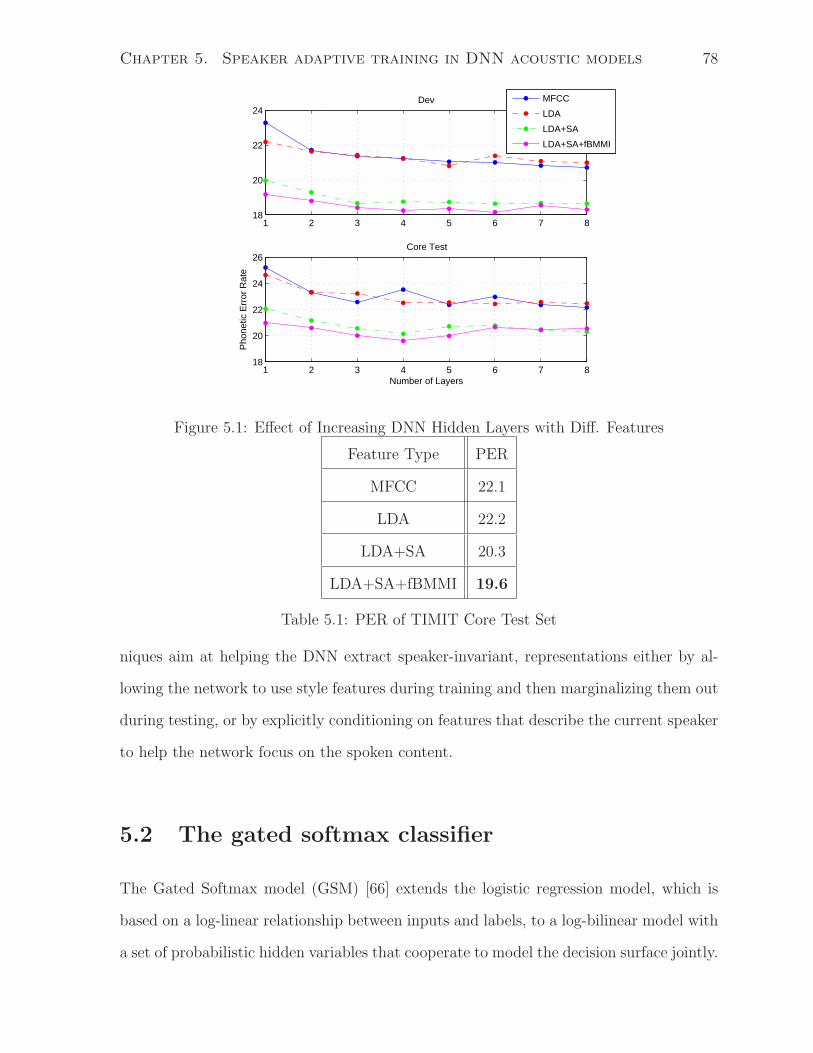
Chapter 5. Speaker adaptive training in DNN acoustic models 78
1 2 3 4 5 6 7 818
20
22
24Dev
1 2 3 4 5 6 7 818
20
22
24
26Core Test
Number of Layers
Pho
netic
Err
or R
ate
MFCC
LDA
LDA+SA
LDA+SA+fBMMI
Figure 5.1: Effect of Increasing DNN Hidden Layers with Diff. Features
Feature Type PER
MFCC 22.1
LDA 22.2
LDA+SA 20.3
LDA+SA+fBMMI 19.6
Table 5.1: PER of TIMIT Core Test Set
niques aim at helping the DNN extract speaker-invariant, representations either by al-
lowing the network to use style features during training and then marginalizing them out
during testing, or by explicitly conditioning on features that describe the current speaker
to help the network focus on the spoken content.
5.2 The gated softmax classifier
The Gated Softmax model (GSM) [66] extends the logistic regression model, which is
based on a log-linear relationship between inputs and labels, to a log-bilinear model with
a set of probabilistic hidden variables that cooperate to model the decision surface jointly.
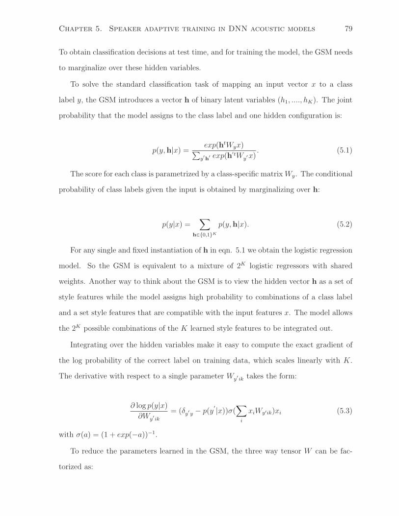
Chapter 5. Speaker adaptive training in DNN acoustic models 79
To obtain classification decisions at test time, and for training the model, the GSM needs
to marginalize over these hidden variables.
To solve the standard classification task of mapping an input vector x to a class
label y, the GSM introduces a vector h of binary latent variables (h1, ...., hK). The joint
probability that the model assigns to the class label and one hidden configuration is:
p(y,h|x) =exp(htWyx)
∑
y′h′ exp(h′tWy
′x). (5.1)
The score for each class is parametrized by a class-specific matrixWy. The conditional
probability of class labels given the input is obtained by marginalizing over h:
p(y|x) =∑
h∈{0,1}K
p(y,h|x). (5.2)
For any single and fixed instantiation of h in eqn. 5.1 we obtain the logistic regression
model. So the GSM is equivalent to a mixture of 2K logistic regressors with shared
weights. Another way to think about the GSM is to view the hidden vector h as a set of
style features while the model assigns high probability to combinations of a class label
and a set style features that are compatible with the input features x. The model allows
the 2K possible combinations of the K learned style features to be integrated out.
Integrating over the hidden variables make it easy to compute the exact gradient of
the log probability of the correct label on training data, which scales linearly with K.
The derivative with respect to a single parameter Wy′ik takes the form:
∂ log p(y|x)
∂Wy′ik
= (δy′y − p(y′
|x))σ(∑
i
xiWy′ik)xi (5.3)
with σ(a) = (1 + exp(−a))−1.
To reduce the parameters learned in the GSM, the three way tensor W can be fac-
torized as:
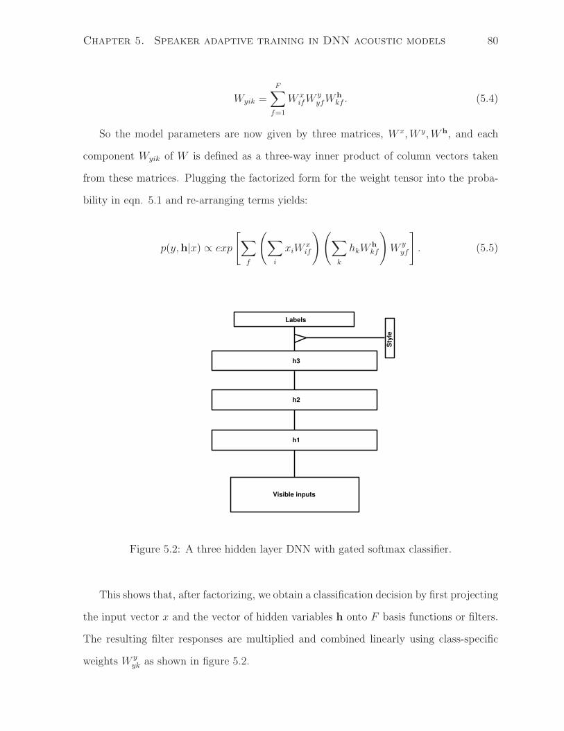
Chapter 5. Speaker adaptive training in DNN acoustic models 80
Wyik =F∑
f=1
W xifW
yyfW
hkf . (5.4)
So the model parameters are now given by three matrices, W x,W y,W h, and each
component Wyik of W is defined as a three-way inner product of column vectors taken
from these matrices. Plugging the factorized form for the weight tensor into the proba-
bility in eqn. 5.1 and re-arranging terms yields:
p(y,h|x) ∝ exp
[
∑
f
(
∑
i
xiWxif
)(
∑
k
hkWhkf
)
W yyf
]
. (5.5)
Figure 5.2: A three hidden layer DNN with gated softmax classifier.
This shows that, after factorizing, we obtain a classification decision by first projecting
the input vector x and the vector of hidden variables h onto F basis functions or filters.
The resulting filter responses are multiplied and combined linearly using class-specific
weights W yyk as shown in figure 5.2.
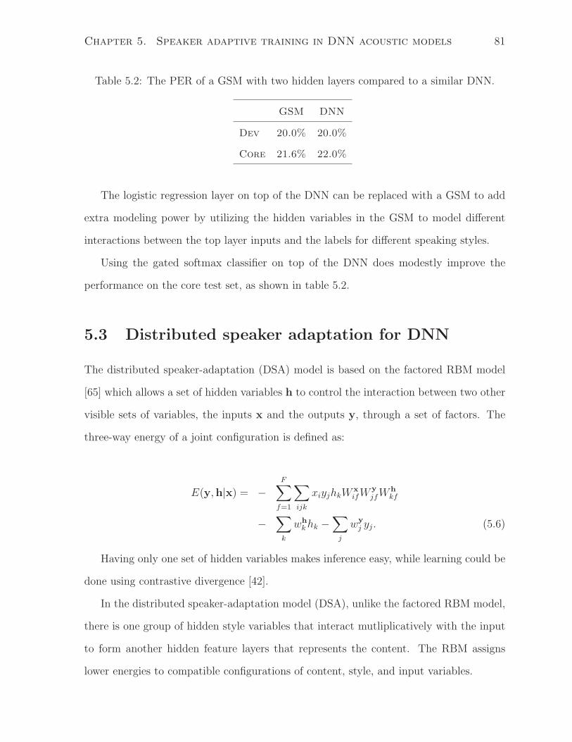
Chapter 5. Speaker adaptive training in DNN acoustic models 81
Table 5.2: The PER of a GSM with two hidden layers compared to a similar DNN.
GSM DNN
Dev 20.0% 20.0%
Core 21.6% 22.0%
The logistic regression layer on top of the DNN can be replaced with a GSM to add
extra modeling power by utilizing the hidden variables in the GSM to model different
interactions between the top layer inputs and the labels for different speaking styles.
Using the gated softmax classifier on top of the DNN does modestly improve the
performance on the core test set, as shown in table 5.2.
5.3 Distributed speaker adaptation for DNN
The distributed speaker-adaptation (DSA) model is based on the factored RBM model
[65] which allows a set of hidden variables h to control the interaction between two other
visible sets of variables, the inputs x and the outputs y, through a set of factors. The
three-way energy of a joint configuration is defined as:
E(y,h|x) = −F∑
f=1
∑
ijk
xiyjhkWxifW
y
jfWhkf
−∑
k
whkhk −
∑
j
wyj yj . (5.6)
Having only one set of hidden variables makes inference easy, while learning could be
done using contrastive divergence [42].
In the distributed speaker-adaptation model (DSA), unlike the factored RBM model,
there is one group of hidden style variables that interact mutliplicatively with the input
to form another hidden feature layers that represents the content. The RBM assigns
lower energies to compatible configurations of content, style, and input variables.
Chapter 5. Speaker adaptive training in DNN acoustic models 82
The learned content hidden features are more invariant to changes in the style of the
input data. The distributed representation of the style features does not require a huge
amount of training data in order to be learned because each style feature focuses on a
single aspect of an input instance and reuses it over all other input instances that have
the same style aspect. This allows for data sharing while learning the style features.
Also, it allows for keeping the number of style features as small as possible, because they
grow linearly with the number of input styles rather than exponentially as in mixture of
experts models. Having distributed style features allows for better generalization of new
input data styles in test scenarios, because any new input style could be composed of the
existing style aspects, i.e., any new style will be modeled by a distribution over existing
styles learned while training.
First the style features are inferred and fixed, then inferring the content features
conditioned on both the input vector and the fixed style features is done. This simplifies
inference, given that there is a way to decide upon the style features. So we need to
learn a set of distributed codes that represent each speaker in the training data and that
generalizes well for new test speakers.
Usually, utterances in the training data are labeled by speaker, or the boundaries
between speakers are given for long conversations. Otherwise, speaker role detection
methods could be used. If we have Ns different speakers in our training data, we could
use this information to train a separate neural network to predict the speaker given a
contextual window of acoustic frames with 1-of-K targets, i.e., K = Ns. We will call it
the speaker network. The visible-to-hidden connections of the network are generatively
pre-trained as an RBM using the contrastive divergence algorithm to get a set of hidden
features that represent both the speaker and the speech which help regularize the network.
Every test speaker is represented using a distribution over the training speakers which
is conditioned on a certain input speech window (about 150ms), so this predicted style
distribution varies, even for the same test speaker, over the acoustic unit that spans
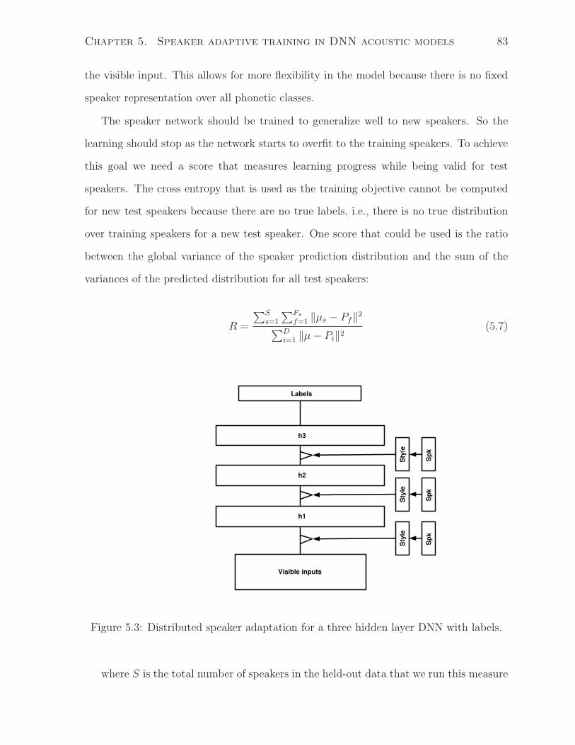
Chapter 5. Speaker adaptive training in DNN acoustic models 83
the visible input. This allows for more flexibility in the model because there is no fixed
speaker representation over all phonetic classes.
The speaker network should be trained to generalize well to new speakers. So the
learning should stop as the network starts to overfit to the training speakers. To achieve
this goal we need a score that measures learning progress while being valid for test
speakers. The cross entropy that is used as the training objective cannot be computed
for new test speakers because there are no true labels, i.e., there is no true distribution
over training speakers for a new test speaker. One score that could be used is the ratio
between the global variance of the speaker prediction distribution and the sum of the
variances of the predicted distribution for all test speakers:
R =
∑S
s=1
∑Fs
f=1 ‖µs − Pf‖2
∑D
i=1 ‖µ− Pi‖2(5.7)
Figure 5.3: Distributed speaker adaptation for a three hidden layer DNN with labels.
where S is the total number of speakers in the held-out data that we run this measure
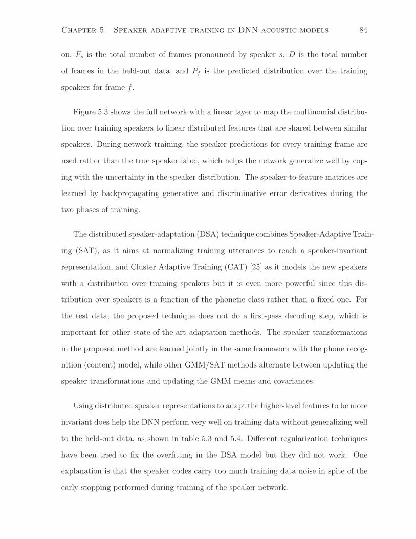
Chapter 5. Speaker adaptive training in DNN acoustic models 84
on, Fs is the total number of frames pronounced by speaker s, D is the total number
of frames in the held-out data, and Pf is the predicted distribution over the training
speakers for frame f .
Figure 5.3 shows the full network with a linear layer to map the multinomial distribu-
tion over training speakers to linear distributed features that are shared between similar
speakers. During network training, the speaker predictions for every training frame are
used rather than the true speaker label, which helps the network generalize well by cop-
ing with the uncertainty in the speaker distribution. The speaker-to-feature matrices are
learned by backpropagating generative and discriminative error derivatives during the
two phases of training.
The distributed speaker-adaptation (DSA) technique combines Speaker-Adaptive Train-
ing (SAT), as it aims at normalizing training utterances to reach a speaker-invariant
representation, and Cluster Adaptive Training (CAT) [25] as it models the new speakers
with a distribution over training speakers but it is even more powerful since this dis-
tribution over speakers is a function of the phonetic class rather than a fixed one. For
the test data, the proposed technique does not do a first-pass decoding step, which is
important for other state-of-the-art adaptation methods. The speaker transformations
in the proposed method are learned jointly in the same framework with the phone recog-
nition (content) model, while other GMM/SAT methods alternate between updating the
speaker transformations and updating the GMM means and covariances.
Using distributed speaker representations to adapt the higher-level features to be more
invariant does help the DNN perform very well on training data without generalizing well
to the held-out data, as shown in table 5.3 and 5.4. Different regularization techniques
have been tried to fix the overfitting in the DSA model but they did not work. One
explanation is that the speaker codes carry too much training data noise in spite of the
early stopping performed during training of the speaker network.
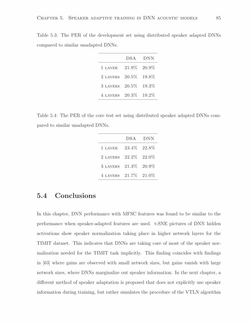
Chapter 5. Speaker adaptive training in DNN acoustic models 85
Table 5.3: The PER of the development set using distributed speaker adapted DNNs
compared to similar unadapted DNNs.
DSA DNN
1 layer 21.9% 20.9%
2 layers 20.5% 19.8%
3 layers 20.5% 19.3%
4 layers 20.3% 19.2%
Table 5.4: The PER of the core test set using distributed speaker adapted DNNs com-
pared to similar unadapted DNNs.
DSA DNN
1 layer 23.4% 22.8%
2 layers 22.2% 22.0%
3 layers 21.3% 20.9%
4 layers 21.7% 21.0%
5.4 Conclusions
In this chapter, DNN performance with MFSC features was found to be similar to the
performance when speaker-adapted features are used. t-SNE pictures of DNN hidden
activations show speaker normalization taking place in higher network layers for the
TIMIT dataset. This indicates that DNNs are taking care of most of the speaker nor-
malization needed for the TIMIT task implicitly. This finding coincides with findings
in [63] where gains are observed with small network sizes, but gains vanish with large
network sizes, where DNNs marginalize out speaker information. In the next chapter, a
different method of speaker adaptation is proposed that does not explicitly use speaker
information during training, but rather simulates the procedure of the VTLN algorithm
Chapter 5. Speaker adaptive training in DNN acoustic models 86
explicitly by using a hand-engineered network structure.
Chapter 6
Convolutional Neural Networks for
acoustic modeling
In previous chapters, DNN acoustic models were shown to achieve very competitive
performance compared to other acoustic models. Using MFSC features as inputs, DNNs
were found to be capable of implicitly normalizing speaker differences in deeper layers
of the network. Each layer of the network learns feature projection weights that aim at
producing the right phone label. The distributed representations used by neural networks
make it easy for DNNs to marginalize out speaker-related aspects in their deeper layers,
focusing only on the spoken content.
Vocal tract length normalization (VTLN) [5,17,61] is one effective way of performing
speaker normalization. It has been found that different people have different vocal tract
lengths which in turn affects formant locations for different sounds. The VTLN algorithm
searches for the best factor to stretch or compress the spectrum by so that different
speakers have formants at similar locations along the frequency axis.
An alternative way to deal with variation in the location of features on the frequency
axis is to replicate feature detectors across a range of similar frequencies. All the replicas
of each feature detector are constrained to have the same weights as each other, but these
87
Chapter 6. Convolutional Neural Networks for acoustic modeling 88
weights can still be learned. Replicating feature detectors does not, by itself, create an
invariant representation in the feature activities because different replicas get activated
when the location of the feature changes. This is an equivariant representation rather
than an invariant one. Replicating a feature detector does, however, ensure that the
knowledge in the weights is the same at all locations across which the feature detector
is replicated. A limited amount of invariance in the vector of feature activations can be
achieved by pooling the outputs of a set of replicated features so that the precise location
of the feature is lost. The range over which the vector of activations is invariant can be
progressively extended by using multiple layers of replicated feature detectors interleaved
with pooling layers. This approach is called “convolutional neural networks” (CNNs) and
has been very successful in computer vision where it is currently the most effective way
to recognize objects in images [49, 54, 56].
6.1 Convolutional Neural Networks (CNNs)
Convolutional Neural Networks (CNNs) [56] introduce three new concepts to the standard
neural networks framework: local filters, weight sharing and pooling. In normal neural
networks, the whole input space is mapped with a different weight vector to each of the
units in the first hidden layer. In CNNs, each hidden activity represents the presence or
absence of a particular feature in a “local” subspace (a patch of contiguous dimensions)
of the input space using a filter, i.e., weight vector, of the same dimensionality as the
input patch. Each filter in the CNN is replicated across the whole input space producing
a “feature map”, i.e., a set of hidden activities, that summarize the presence or absence
of one feature type over all local locations in the input space. “Weight sharing” refers to
the idea that all hidden units forming one feature map share the same filter, i.e., weight
vector. The first layer of a CNN where shared weights are applied to generate many
feature maps is called a “convolutional layer” because the filter is convolved with the
Chapter 6. Convolutional Neural Networks for acoustic modeling 89
input. Actually it is only a convolution if the “stride” by which a filter is translated to
be applied to the next patch is 1. “Convolutional” nets often use a stride greater than 1.
To deal with the fact that objects in the input space do not always appear in the same
location, CNNs use a mechanism called “pooling” to subsample feature maps produced
by the convolutional layer in order to generate lower-resolution feature maps, which can
tolerate small changes in the feature location without any change in the subsampled
representations. Examples of pooling operators are the maximum or the average over a
certain pooling window of input feature map from the convolutional layer. This stage of
a CNN is called the subsampling or pooling layer.
The combination of these three new concepts provides tolerance to minor translations
of object parts. Higher convolutional layers could use broader filters, acting on lower
resolution inputs to produce more complex representations of the input. After a few pairs
of convolutional and pooling layers, fully connected layers (as in normal neural networks)
are typically used to combine these complex representations to perform classification
using a final softmax layer.
This hierarchical structure of CNNs was found to be key for producing the best
performing systems over many image processing and vision tasks [49, 54, 56,57].
CNNs have been applied to speech recognition before [51, 55, 59], with convolution
and pooling operations taking place over the time axis. DNNs already perform temporal
convolution, as they are applied to successive windows of frames when scanning the input
utterance, as proposed by [51]. When applied over the time domain, CNNs perform
convolutions not only in the input layer but also in all subsequent hidden layers. Also
CNNs offer pooling as a means to account for small temporal shifts.
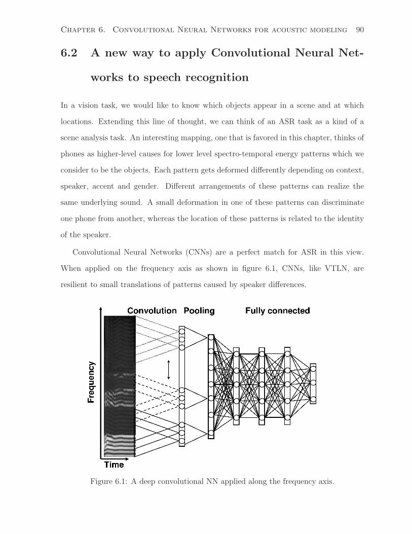
Chapter 6. Convolutional Neural Networks for acoustic modeling 90
6.2 A new way to apply Convolutional Neural Net-
works to speech recognition
In a vision task, we would like to know which objects appear in a scene and at which
locations. Extending this line of thought, we can think of an ASR task as a kind of a
scene analysis task. An interesting mapping, one that is favored in this chapter, thinks of
phones as higher-level causes for lower level spectro-temporal energy patterns which we
consider to be the objects. Each pattern gets deformed differently depending on context,
speaker, accent and gender. Different arrangements of these patterns can realize the
same underlying sound. A small deformation in one of these patterns can discriminate
one phone from another, whereas the location of these patterns is related to the identity
of the speaker.
Convolutional Neural Networks (CNNs) are a perfect match for ASR in this view.
When applied on the frequency axis as shown in figure 6.1, CNNs, like VTLN, are
resilient to small translations of patterns caused by speaker differences.
Figure 6.1: A deep convolutional NN applied along the frequency axis.
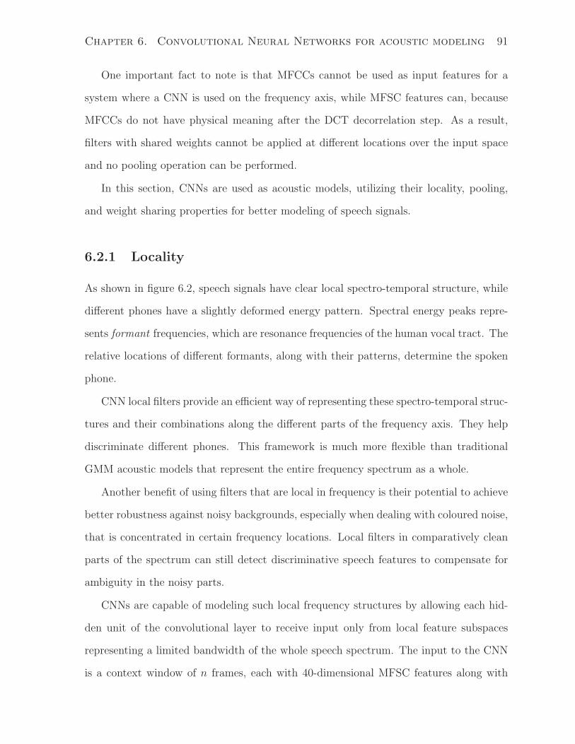
Chapter 6. Convolutional Neural Networks for acoustic modeling 91
One important fact to note is that MFCCs cannot be used as input features for a
system where a CNN is used on the frequency axis, while MFSC features can, because
MFCCs do not have physical meaning after the DCT decorrelation step. As a result,
filters with shared weights cannot be applied at different locations over the input space
and no pooling operation can be performed.
In this section, CNNs are used as acoustic models, utilizing their locality, pooling,
and weight sharing properties for better modeling of speech signals.
6.2.1 Locality
As shown in figure 6.2, speech signals have clear local spectro-temporal structure, while
different phones have a slightly deformed energy pattern. Spectral energy peaks repre-
sents formant frequencies, which are resonance frequencies of the human vocal tract. The
relative locations of different formants, along with their patterns, determine the spoken
phone.
CNN local filters provide an efficient way of representing these spectro-temporal struc-
tures and their combinations along the different parts of the frequency axis. They help
discriminate different phones. This framework is much more flexible than traditional
GMM acoustic models that represent the entire frequency spectrum as a whole.
Another benefit of using filters that are local in frequency is their potential to achieve
better robustness against noisy backgrounds, especially when dealing with coloured noise,
that is concentrated in certain frequency locations. Local filters in comparatively clean
parts of the spectrum can still detect discriminative speech features to compensate for
ambiguity in the noisy parts.
CNNs are capable of modeling such local frequency structures by allowing each hid-
den unit of the convolutional layer to receive input only from local feature subspaces
representing a limited bandwidth of the whole speech spectrum. The input to the CNN
is a context window of n frames, each with 40-dimensional MFSC features along with
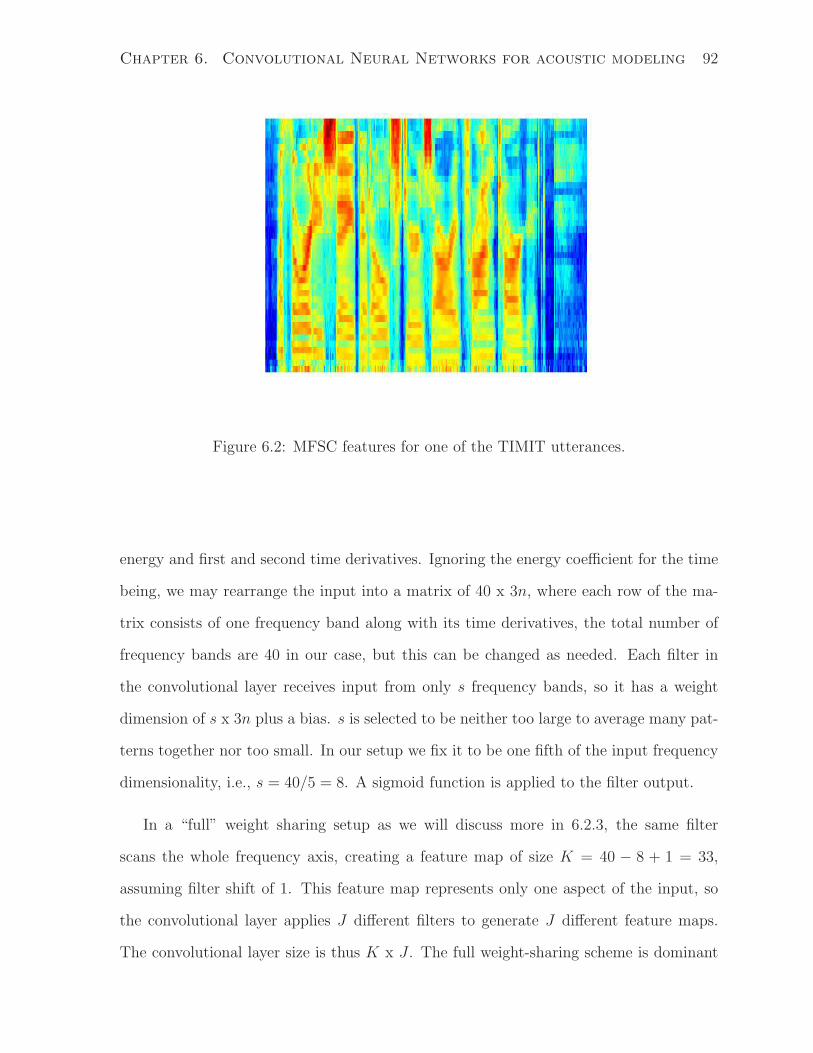
Chapter 6. Convolutional Neural Networks for acoustic modeling 92
Figure 6.2: MFSC features for one of the TIMIT utterances.
energy and first and second time derivatives. Ignoring the energy coefficient for the time
being, we may rearrange the input into a matrix of 40 x 3n, where each row of the ma-
trix consists of one frequency band along with its time derivatives, the total number of
frequency bands are 40 in our case, but this can be changed as needed. Each filter in
the convolutional layer receives input from only s frequency bands, so it has a weight
dimension of s x 3n plus a bias. s is selected to be neither too large to average many pat-
terns together nor too small. In our setup we fix it to be one fifth of the input frequency
dimensionality, i.e., s = 40/5 = 8. A sigmoid function is applied to the filter output.
In a “full” weight sharing setup as we will discuss more in 6.2.3, the same filter
scans the whole frequency axis, creating a feature map of size K = 40 − 8 + 1 = 33,
assuming filter shift of 1. This feature map represents only one aspect of the input, so
the convolutional layer applies J different filters to generate J different feature maps.
The convolutional layer size is thus K x J . The full weight-sharing scheme is dominant
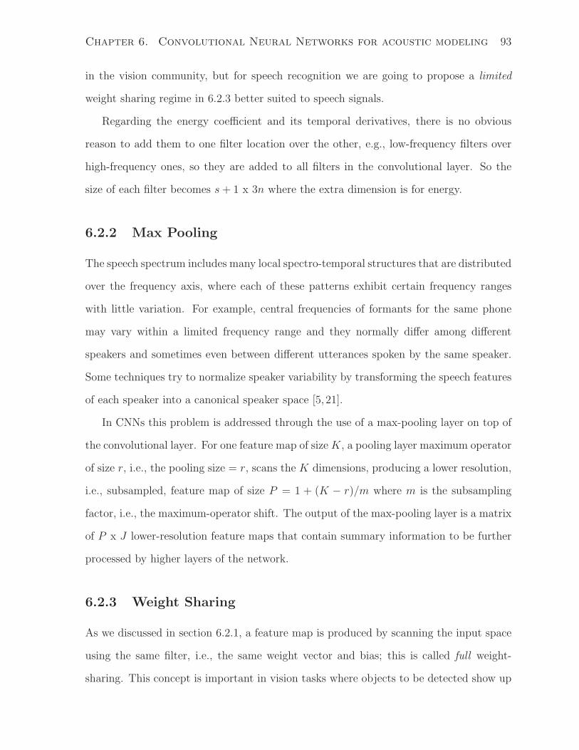
Chapter 6. Convolutional Neural Networks for acoustic modeling 93
in the vision community, but for speech recognition we are going to propose a limited
weight sharing regime in 6.2.3 better suited to speech signals.
Regarding the energy coefficient and its temporal derivatives, there is no obvious
reason to add them to one filter location over the other, e.g., low-frequency filters over
high-frequency ones, so they are added to all filters in the convolutional layer. So the
size of each filter becomes s+ 1 x 3n where the extra dimension is for energy.
6.2.2 Max Pooling
The speech spectrum includes many local spectro-temporal structures that are distributed
over the frequency axis, where each of these patterns exhibit certain frequency ranges
with little variation. For example, central frequencies of formants for the same phone
may vary within a limited frequency range and they normally differ among different
speakers and sometimes even between different utterances spoken by the same speaker.
Some techniques try to normalize speaker variability by transforming the speech features
of each speaker into a canonical speaker space [5, 21].
In CNNs this problem is addressed through the use of a max-pooling layer on top of
the convolutional layer. For one feature map of sizeK, a pooling layer maximum operator
of size r, i.e., the pooling size = r, scans the K dimensions, producing a lower resolution,
i.e., subsampled, feature map of size P = 1 + (K − r)/m where m is the subsampling
factor, i.e., the maximum-operator shift. The output of the max-pooling layer is a matrix
of P x J lower-resolution feature maps that contain summary information to be further
processed by higher layers of the network.
6.2.3 Weight Sharing
As we discussed in section 6.2.1, a feature map is produced by scanning the input space
using the same filter, i.e., the same weight vector and bias; this is called full weight-
sharing. This concept is important in vision tasks where objects to be detected show up
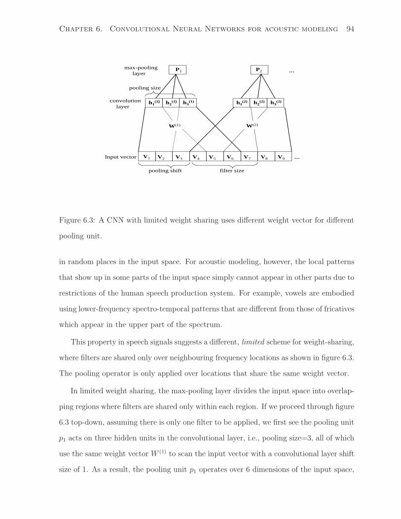
Chapter 6. Convolutional Neural Networks for acoustic modeling 94
V1 …
h1(1)
P2
h2(1) h3
(1) h1(2) h2
(2) h3(2)
…
W(2)W(1)
pooling shift filter size
P1
V2 V3 V4 V5 V6 V7 V8 V9
pooling size
convolutionlayer
Input vector
max-poolinglayer
Figure 6.3: A CNN with limited weight sharing uses different weight vector for different
pooling unit.
in random places in the input space. For acoustic modeling, however, the local patterns
that show up in some parts of the input space simply cannot appear in other parts due to
restrictions of the human speech production system. For example, vowels are embodied
using lower-frequency spectro-temporal patterns that are different from those of fricatives
which appear in the upper part of the spectrum.
This property in speech signals suggests a different, limited scheme for weight-sharing,
where filters are shared only over neighbouring frequency locations as shown in figure 6.3.
The pooling operator is only applied over locations that share the same weight vector.
In limited weight sharing, the max-pooling layer divides the input space into overlap-
ping regions where filters are shared only within each region. If we proceed through figure
6.3 top-down, assuming there is only one filter to be applied, we first see the pooling unit
p1 acts on three hidden units in the convolutional layer, i.e., pooling size=3, all of which
use the same weight vector W (1) to scan the input vector with a convolutional layer shift
size of 1. As a result, the pooling unit p1 operates over 6 dimensions of the input space,
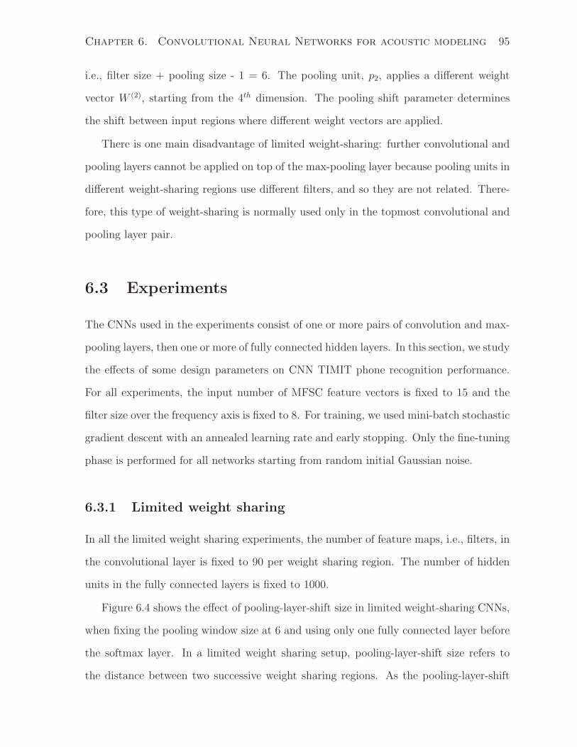
Chapter 6. Convolutional Neural Networks for acoustic modeling 95
i.e., filter size + pooling size - 1 = 6. The pooling unit, p2, applies a different weight
vector W (2), starting from the 4th dimension. The pooling shift parameter determines
the shift between input regions where different weight vectors are applied.
There is one main disadvantage of limited weight-sharing: further convolutional and
pooling layers cannot be applied on top of the max-pooling layer because pooling units in
different weight-sharing regions use different filters, and so they are not related. There-
fore, this type of weight-sharing is normally used only in the topmost convolutional and
pooling layer pair.
6.3 Experiments
The CNNs used in the experiments consist of one or more pairs of convolution and max-
pooling layers, then one or more of fully connected hidden layers. In this section, we study
the effects of some design parameters on CNN TIMIT phone recognition performance.
For all experiments, the input number of MFSC feature vectors is fixed to 15 and the
filter size over the frequency axis is fixed to 8. For training, we used mini-batch stochastic
gradient descent with an annealed learning rate and early stopping. Only the fine-tuning
phase is performed for all networks starting from random initial Gaussian noise.
6.3.1 Limited weight sharing
In all the limited weight sharing experiments, the number of feature maps, i.e., filters, in
the convolutional layer is fixed to 90 per weight sharing region. The number of hidden
units in the fully connected layers is fixed to 1000.
Figure 6.4 shows the effect of pooling-layer-shift size in limited weight-sharing CNNs,
when fixing the pooling window size at 6 and using only one fully connected layer before
the softmax layer. In a limited weight sharing setup, pooling-layer-shift size refers to
the distance between two successive weight sharing regions. As the pooling-layer-shift
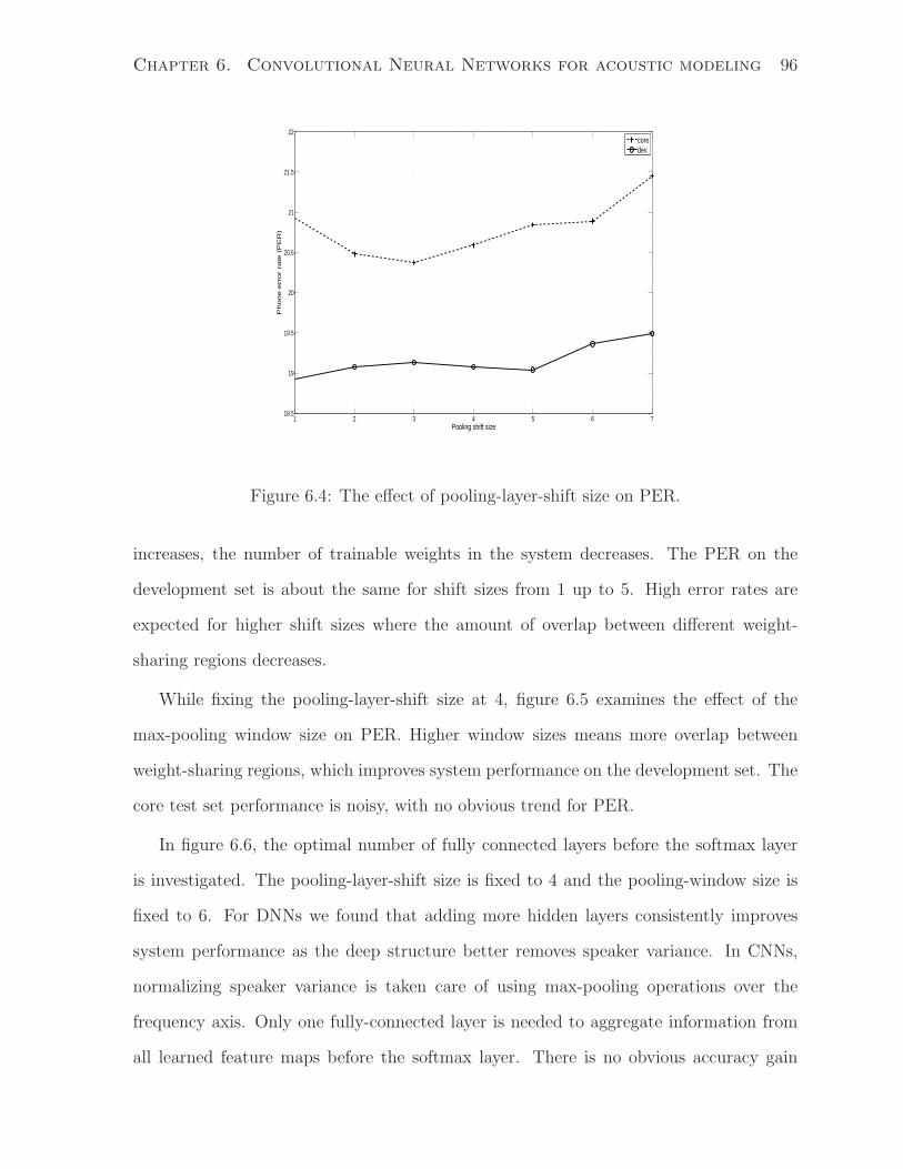
Chapter 6. Convolutional Neural Networks for acoustic modeling 96
1 2 3 4 5 6 718.5
19
19.5
20
20.5
21
21.5
22
Pooling shift size
Ph
on
e e
rro
r ra
te (
PE
R)
coredev
Figure 6.4: The effect of pooling-layer-shift size on PER.
increases, the number of trainable weights in the system decreases. The PER on the
development set is about the same for shift sizes from 1 up to 5. High error rates are
expected for higher shift sizes where the amount of overlap between different weight-
sharing regions decreases.
While fixing the pooling-layer-shift size at 4, figure 6.5 examines the effect of the
max-pooling window size on PER. Higher window sizes means more overlap between
weight-sharing regions, which improves system performance on the development set. The
core test set performance is noisy, with no obvious trend for PER.
In figure 6.6, the optimal number of fully connected layers before the softmax layer
is investigated. The pooling-layer-shift size is fixed to 4 and the pooling-window size is
fixed to 6. For DNNs we found that adding more hidden layers consistently improves
system performance as the deep structure better removes speaker variance. In CNNs,
normalizing speaker variance is taken care of using max-pooling operations over the
frequency axis. Only one fully-connected layer is needed to aggregate information from
all learned feature maps before the softmax layer. There is no obvious accuracy gain
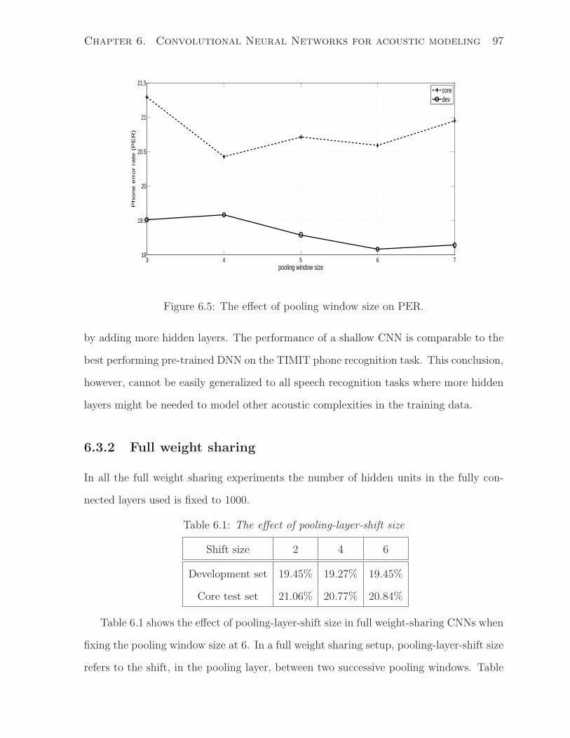
Chapter 6. Convolutional Neural Networks for acoustic modeling 97
3 4 5 6 719
19.5
20
20.5
21
21.5
pooling window size
Ph
on
e e
rro
r ra
te (
PE
R)
coredev
Figure 6.5: The effect of pooling window size on PER.
by adding more hidden layers. The performance of a shallow CNN is comparable to the
best performing pre-trained DNN on the TIMIT phone recognition task. This conclusion,
however, cannot be easily generalized to all speech recognition tasks where more hidden
layers might be needed to model other acoustic complexities in the training data.
6.3.2 Full weight sharing
In all the full weight sharing experiments the number of hidden units in the fully con-
nected layers used is fixed to 1000.
Table 6.1: The effect of pooling-layer-shift size
Shift size 2 4 6
Development set 19.45% 19.27% 19.45%
Core test set 21.06% 20.77% 20.84%
Table 6.1 shows the effect of pooling-layer-shift size in full weight-sharing CNNs when
fixing the pooling window size at 6. In a full weight sharing setup, pooling-layer-shift size
refers to the shift, in the pooling layer, between two successive pooling windows. Table
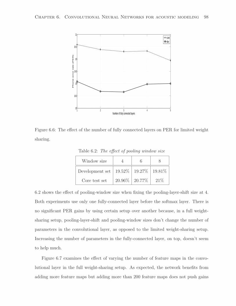
Chapter 6. Convolutional Neural Networks for acoustic modeling 98
1 2 3 4 518
18.5
19
19.5
20
20.5
21
Number of fully connected layers
Ph
on
e e
rro
r ra
te
(P
ER
)
coredev
Figure 6.6: The effect of the number of fully connected layers on PER for limited weight
sharing.
Table 6.2: The effect of pooling window size
Window size 4 6 8
Development set 19.52% 19.27% 19.81%
Core test set 20.96% 20.77% 21%
6.2 shows the effect of pooling-window size when fixing the pooling-layer-shift size at 4.
Both experiments use only one fully-connected layer before the softmax layer. There is
no significant PER gains by using certain setup over another because, in a full weight-
sharing setup, pooling-layer-shift and pooling-window sizes don’t change the number of
parameters in the convolutional layer, as opposed to the limited weight-sharing setup.
Increasing the number of parameters in the fully-connected layer, on top, doesn’t seem
to help much.
Figure 6.7 examines the effect of varying the number of feature maps in the convo-
lutional layer in the full weight-sharing setup. As expected, the network benefits from
adding more feature maps but adding more than 200 feature maps does not push gains
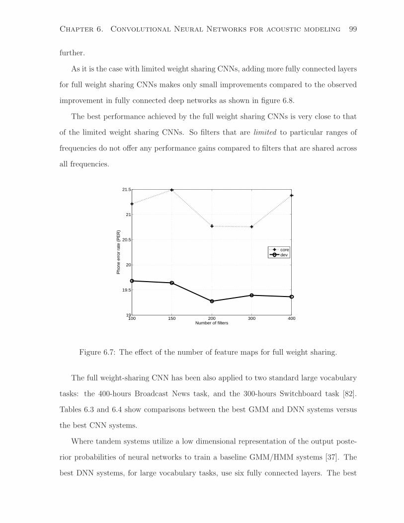
Chapter 6. Convolutional Neural Networks for acoustic modeling 99
further.
As it is the case with limited weight sharing CNNs, adding more fully connected layers
for full weight sharing CNNs makes only small improvements compared to the observed
improvement in fully connected deep networks as shown in figure 6.8.
The best performance achieved by the full weight sharing CNNs is very close to that
of the limited weight sharing CNNs. So filters that are limited to particular ranges of
frequencies do not offer any performance gains compared to filters that are shared across
all frequencies.
100 150 200 300 40019
19.5
20
20.5
21
21.5
Number of filters
Pho
ne e
rror
rat
e (P
ER
)
coredev
Figure 6.7: The effect of the number of feature maps for full weight sharing.
The full weight-sharing CNN has been also applied to two standard large vocabulary
tasks: the 400-hours Broadcast News task, and the 300-hours Switchboard task [82].
Tables 6.3 and 6.4 show comparisons between the best GMM and DNN systems versus
the best CNN systems.
Where tandem systems utilize a low dimensional representation of the output poste-
rior probabilities of neural networks to train a baseline GMM/HMM systems [37]. The
best DNN systems, for large vocabulary tasks, use six fully connected layers. The best
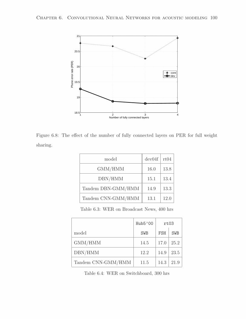
Chapter 6. Convolutional Neural Networks for acoustic modeling 100
1 2 3 418.5
19
19.5
20
20.5
21
Number of fully connected layers
Pho
ne e
rror
rat
e (P
ER
)
coredev
Figure 6.8: The effect of the number of fully connected layers on PER for full weight
sharing.
model dev04f rt04
GMM/HMM 16.0 13.8
DBN/HMM 15.1 13.4
Tandem DBN-GMM/HMM 14.9 13.3
Tandem CNN-GMM/HMM 13.1 12.0
Table 6.3: WER on Broadcast News, 400 hrs
Hub5’00 rt03
model SWB FSH SWB
GMM/HMM 14.5 17.0 25.2
DBN/HMM 12.2 14.9 23.5
Tandem CNN-GMM/HMM 11.5 14.3 21.9
Table 6.4: WER on Switchboard, 300 hrs
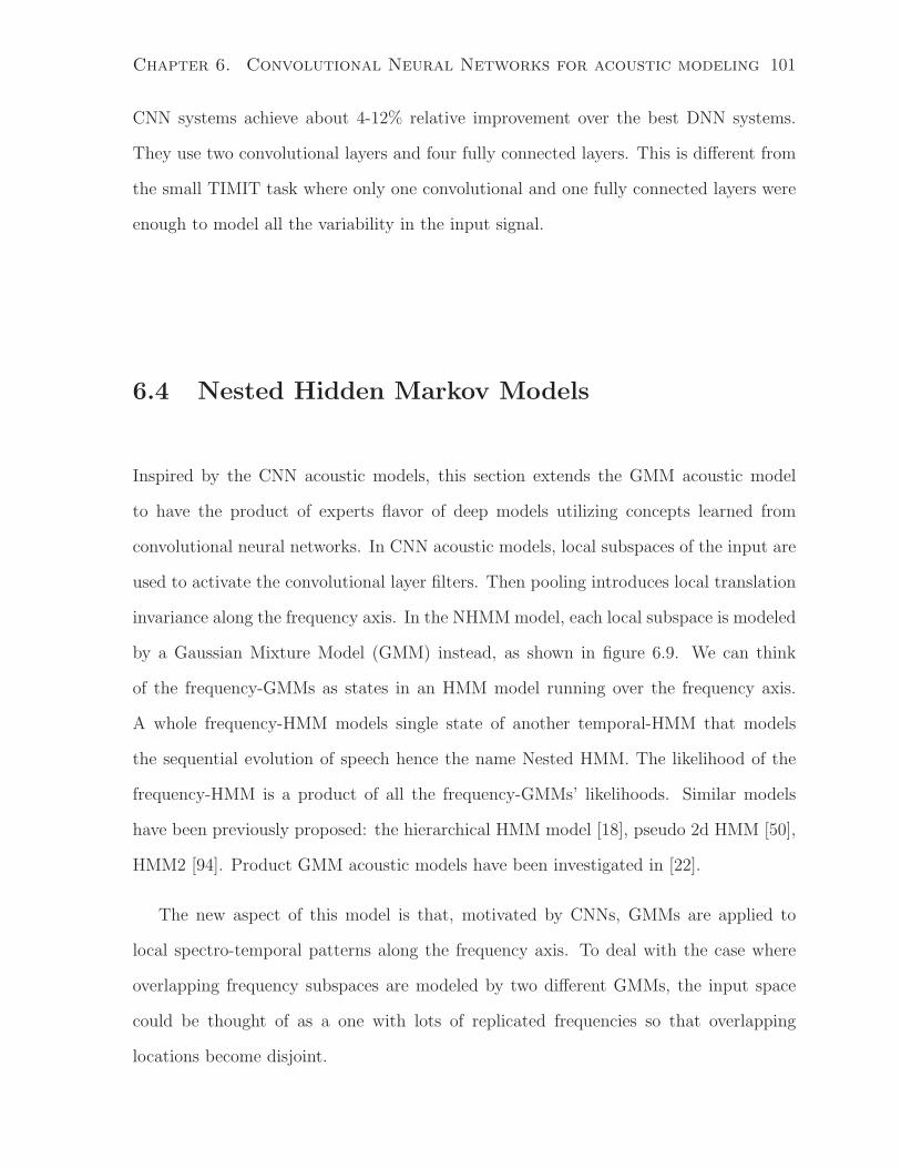
Chapter 6. Convolutional Neural Networks for acoustic modeling 101
CNN systems achieve about 4-12% relative improvement over the best DNN systems.
They use two convolutional layers and four fully connected layers. This is different from
the small TIMIT task where only one convolutional and one fully connected layers were
enough to model all the variability in the input signal.
6.4 Nested Hidden Markov Models
Inspired by the CNN acoustic models, this section extends the GMM acoustic model
to have the product of experts flavor of deep models utilizing concepts learned from
convolutional neural networks. In CNN acoustic models, local subspaces of the input are
used to activate the convolutional layer filters. Then pooling introduces local translation
invariance along the frequency axis. In the NHMM model, each local subspace is modeled
by a Gaussian Mixture Model (GMM) instead, as shown in figure 6.9. We can think
of the frequency-GMMs as states in an HMM model running over the frequency axis.
A whole frequency-HMM models single state of another temporal-HMM that models
the sequential evolution of speech hence the name Nested HMM. The likelihood of the
frequency-HMM is a product of all the frequency-GMMs’ likelihoods. Similar models
have been previously proposed: the hierarchical HMM model [18], pseudo 2d HMM [50],
HMM2 [94]. Product GMM acoustic models have been investigated in [22].
The new aspect of this model is that, motivated by CNNs, GMMs are applied to
local spectro-temporal patterns along the frequency axis. To deal with the case where
overlapping frequency subspaces are modeled by two different GMMs, the input space
could be thought of as a one with lots of replicated frequencies so that overlapping
locations become disjoint.
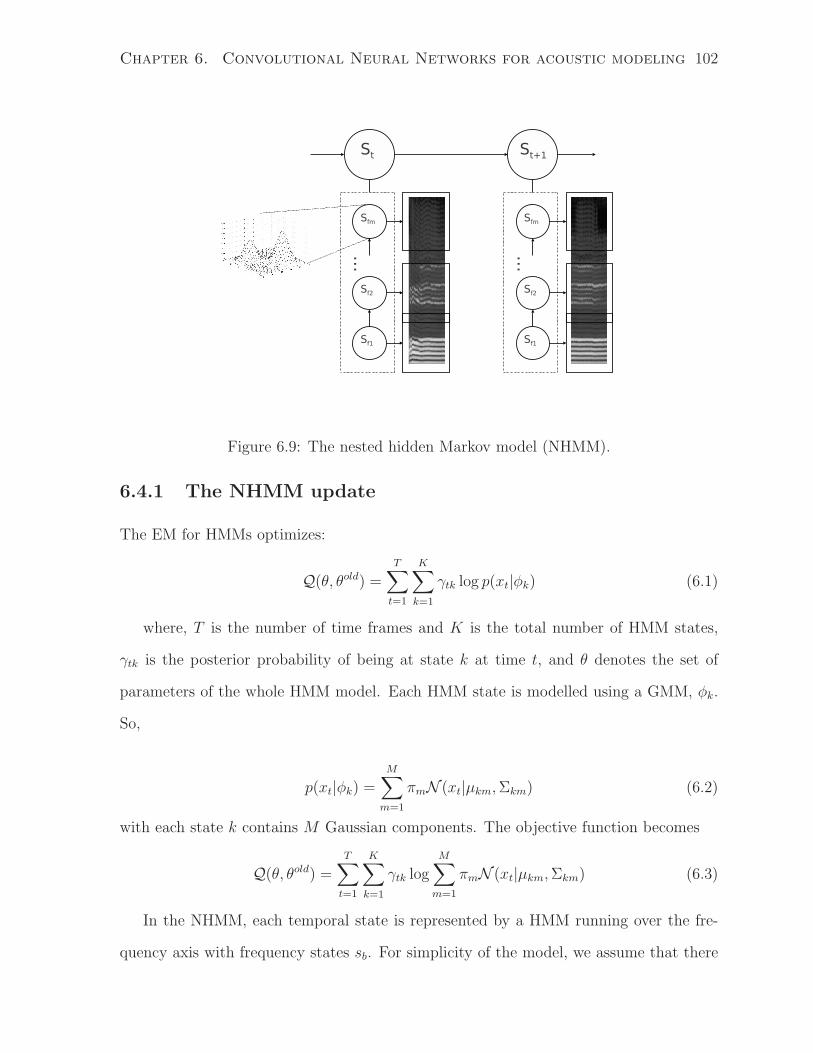
Chapter 6. Convolutional Neural Networks for acoustic modeling 102
Figure 6.9: The nested hidden Markov model (NHMM).
6.4.1 The NHMM update
The EM for HMMs optimizes:
Q(θ, θold) =T∑
t=1
K∑
k=1
γtk log p(xt|φk) (6.1)
where, T is the number of time frames and K is the total number of HMM states,
γtk is the posterior probability of being at state k at time t, and θ denotes the set of
parameters of the whole HMM model. Each HMM state is modelled using a GMM, φk.
So,
p(xt|φk) =M∑
m=1
πmN (xt|µkm,Σkm) (6.2)
with each state k contains M Gaussian components. The objective function becomes
Q(θ, θold) =T∑
t=1
K∑
k=1
γtk logM∑
m=1
πmN (xt|µkm,Σkm) (6.3)
In the NHMM, each temporal state is represented by a HMM running over the fre-
quency axis with frequency states sb. For simplicity of the model, we assume that there
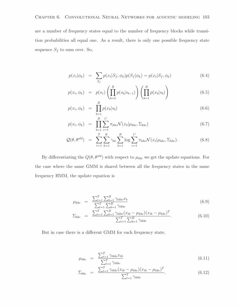
Chapter 6. Convolutional Neural Networks for acoustic modeling 103
are a number of frequency states equal to the number of frequency blocks while transi-
tion probabilities all equal one. As a result, there is only one possible frequency state
sequence Sf to sum over. So,
p(xt|φk) =∑
Sf
p(xt|Sf , φk)p(Sf |φk) = p(xt|Sf , φk) (6.4)
p(xt, φk) = p(s1)
(
B∏
b=2
p(sb|sb−1)
)(
B∏
b=1
p(xb|sb)
)
(6.5)
p(xt, φk) =B∏
b=1
p(xb|sb) (6.6)
p(xt, φk) =B∏
b=1
C∑
c=1
πkbcN (xb|µkbc,Σkbc) (6.7)
Q(θ, θold) =T∑
t=1
K∑
k=1
γtk
B∑
b=1
logC∑
c=1
πkbcN (xt|µkbc,Σkbc). (6.8)
By differentiating the Q(θ, θold) with respect to µkbc we get the update equations. For
the case where the same GMM is shared between all the frequency states in the same
frequency HMM, the update equation is
µkbc =
∑T
t=1
∑B
b=1 γtkbcxb∑T
t=1
∑B
b=1 γtkbc(6.9)
Σkbc =
∑T
t=1
∑B
b=1 γtkbc(xtb − µkbc)(xtb − µkbc)T
∑T
t=1
∑B
b=1 γtkbc. (6.10)
But in case there is a different GMM for each frequency state,
µkbc =
∑T
t=1 γtkbcxtb∑T
t=1 γtkbc(6.11)
Σkbc =
∑T
t=1 γtkbc(xtb − µkbc)(xtb − µkbc)T
∑T
t=1 γtkbc. (6.12)
Chapter 6. Convolutional Neural Networks for acoustic modeling 104
6.4.2 Experiments
In this section, we show preliminary experiments of the NHMM versus the baseline model
with the whole frequency space represented by a single GMM. A separate model is esti-
mated for each monophone state so there are 183 total models in each system. Diagonal
covariance GMMs are used for both the NHMM and baseline. Mean and variance nor-
malized MFSC features are used with a context window of 9 frames as inputs. The
frequency axis is split into overlapping local subspaces then linear discriminant analysis
(LDA) is applied to reduce the input vector dimensionality for robust GMM estimation.
One problem we discovered while training the NHMM acoustic model is that for some
frequency states the posterior probabilities over Gaussian components in that GMM are
uniform. This happens in the high frequency states in vowels where all the activities
are taking place in the lower part of the spectrum while the upper part is almost always
empty. Another related point is that the NHMM model, as a product of many GMMs,
represents a single GMM with exponential number of components resulting from the cross
product of all Gaussian components in each frequency location. Many of these resulting
components are unnecessary and they appear at weird locations in the acoustic space.
To get rid of these unnecessary components, a max approximation is used instead of the
sum in the GMM model. Only one component is active for each input observation while
all the other components have zero responsibility.
Also, we needed to adjust the scale of the resulting NHMM likelihood to fit into the
same dynamic range of the baseline in order not to have to readjust the language model
scaling factor and decoder pruning parameters. Table 6.5 shows that the performance of
the NHMM acoustic model on the TIMIT core test set is about the same as that of the
baseline system.
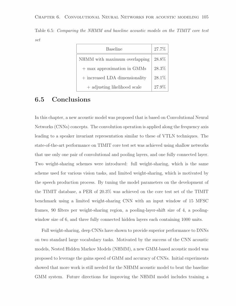
Chapter 6. Convolutional Neural Networks for acoustic modeling 105
Table 6.5: Comparing the NHMM and baseline acoustic models on the TIMIT core test
set
Baseline 27.7%
NHMM with maximum overlapping 28.8%
+ max approximation in GMMs 28.3%
+ increased LDA dimensionality 28.1%
+ adjusting likelihood scale 27.9%
6.5 Conclusions
In this chapter, a new acoustic model was proposed that is based on Convolutional Neural
Networks (CNNs) concepts. The convolution operation is applied along the frequency axis
leading to a speaker invariant representation similar to these of VTLN techniques. The
state-of-the-art performance on TIMIT core test set was achieved using shallow networks
that use only one pair of convolutional and pooling layers, and one fully connected layer.
Two weight-sharing schemes were introduced: full weight-sharing, which is the same
scheme used for various vision tasks, and limited weight-sharing, which is motivated by
the speech production process. By tuning the model parameters on the development of
the TIMIT database, a PER of 20.3% was achieved on the core test set of the TIMIT
benchmark using a limited weight-sharing CNN with an input window of 15 MFSC
frames, 90 filters per weight-sharing region, a pooling-layer-shift size of 4, a pooling-
window size of 6, and three fully connected hidden layers each containing 1000 units.
Full weight-sharing, deep CNNs have shown to provide superior performance to DNNs
on two standard large vocabulary tasks. Motivated by the success of the CNN acoustic
models, Nested Hidden Markov Models (NHMM), a new GMM-based acoustic model was
proposed to leverage the gains speed of GMM and accuracy of CNNs. Initial experiments
showed that more work is still needed for the NHMM acoustic model to beat the baseline
GMM system. Future directions for improving the NHMM model includes training a
Chapter 6. Convolutional Neural Networks for acoustic modeling 106
proper HMM along the frequency axis and training another module on top of the NHMM,
e.g. an RBM, to remove the useless Gaussian components.
Chapter 7
Conclusions and future directions
In this thesis a new acoustic model that is based on Deep Neural Networks (DNNs) was
presented and a new state of the art phone recognition accuracy was reported using deep
models. The depth of the model is used to normalize out speaker differences. This was
demonstrated using t-SNE visualizations for similar utterances pronounced by different
speakers. The visualizations show that DNNs are capable of marginalizing out speaker
variation while focusing on the spoken content. The performance of DNNs using MFSC
features was found to be similar to the performance using other speaker-adapted features.
Using our understanding of how DNNs perform implicit speaker adaptation, DNNs
can be designed in a way that takes care of speaker differences explicitly through network
structure. Using Convolutional Neural Networks (CNNs) that perform the convolution
operation over the frequency axis, state-of-the-art performance was achieved with a shal-
low architecture. The proposed limited weight-sharing CNN system could be considered
as a hybrid of knowledge based systems and statistical systems, where we used our un-
derstanding of the structure of the speech spectrum to share parameters locally and have
different sets of parameters for different locations in the spectrum, while allowing the
network to learn the kind of features that it likes at each of these locations.
If we know how exactly a DNN acoustic model works along with domain experience in
107
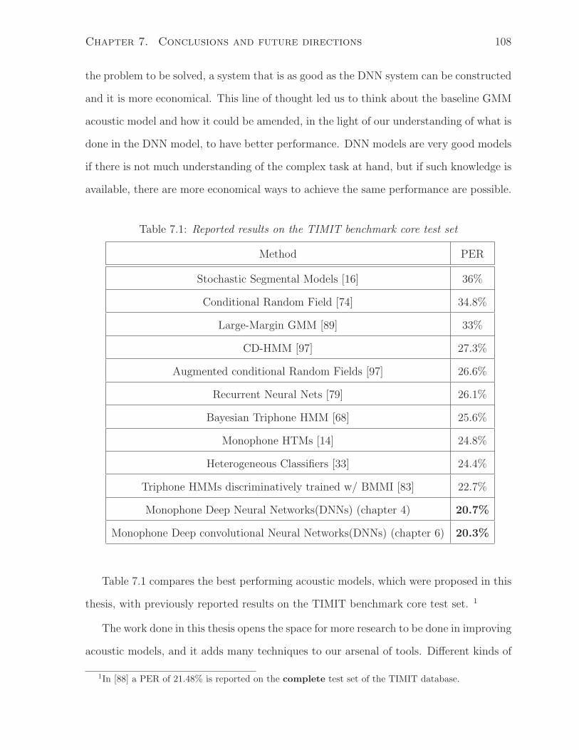
Chapter 7. Conclusions and future directions 108
the problem to be solved, a system that is as good as the DNN system can be constructed
and it is more economical. This line of thought led us to think about the baseline GMM
acoustic model and how it could be amended, in the light of our understanding of what is
done in the DNN model, to have better performance. DNN models are very good models
if there is not much understanding of the complex task at hand, but if such knowledge is
available, there are more economical ways to achieve the same performance are possible.
Table 7.1: Reported results on the TIMIT benchmark core test set
Method PER
Stochastic Segmental Models [16] 36%
Conditional Random Field [74] 34.8%
Large-Margin GMM [89] 33%
CD-HMM [97] 27.3%
Augmented conditional Random Fields [97] 26.6%
Recurrent Neural Nets [79] 26.1%
Bayesian Triphone HMM [68] 25.6%
Monophone HTMs [14] 24.8%
Heterogeneous Classifiers [33] 24.4%
Triphone HMMs discriminatively trained w/ BMMI [83] 22.7%
Monophone Deep Neural Networks(DNNs) (chapter 4) 20.7%
Monophone Deep convolutional Neural Networks(DNNs) (chapter 6) 20.3%
Table 7.1 compares the best performing acoustic models, which were proposed in this
thesis, with previously reported results on the TIMIT benchmark core test set. 1
The work done in this thesis opens the space for more research to be done in improving
acoustic models, and it adds many techniques to our arsenal of tools. Different kinds of
1In [88] a PER of 21.48% is reported on the complete test set of the TIMIT database.
Chapter 7. Conclusions and future directions 109
binary, discrete, and continuous features were used in the past for NN acoustic model
training. In DNN models, features could be combined in the input layer or later in
subsequent higher layers. Also pre-training of DNN acoustic models was found not to
be necessary for training deep models; however, it is expected to play an important role
in tasks where tiny amounts of data are available, and also in cases where we want to
utilize the huge amounts of unlabelled spoken data currently available. Further work is
still needed to develop pre-training techniques that are faster than the existing ones.
CNN acoustic models need more research along multiple directions. First, we need
to improve our understanding of how deep CNN models interact with other feature-
based speaker adaptation techniques and whether they replace or complement each other.
Although limited weight sharing did not provide improvement over a multi-layer CNN
with full weight sharing [84], limited weight sharing can be seen as a generalization
of the mel-frequency spectral coefficients applied to the FFT features in the process of
generating MFSC features. Hence, it could be used in CNNs for extracting richer features
from high dimensional spectral input [85]. One other direction for further improvement is
to use convolution and pooling layers in tandem with fully connected layers with temporal
connections. This way the lower part of the network acts more like the ears of the system,
while the upper part acts like the brain which aggregates information across time over
multiple layers to produce the best output prediction.
Speaker adaptation for DNN acoustic models is another rich area for further improve-
ment. One extension of the Distributed Speaker Adaptation (DSA) technique introduced
in chapter 5 is to use the GMM first order statistics, as in [13], to learn speaker codes
in the speaker NN. Another possibility is to train the speaker NN and the main DNN
jointly. Some recent work that is along the same lines has been introduced. In [86], iden-
tity vectors (i-vectors) as described in [13] are fed to the DNN while training, while [1]
uses the backpropagation algorithm to learn the speaker codes.
Motivated by the recent success in unsupervised phonetic-units learning and pronun-
Chapter 7. Conclusions and future directions 110
ciation modelling [58] and the successes of recurrent neural networks (RNNs) in acoustic
modelling [30] and language modelling [67], one important future direction is to build a
giant neural network that does phonetic-units learning, acoustic modelling, pronunciation
modelling, and language modelling jointly.
Bibliography
[1] Ossama Abdel-Hamid and Hui Jiang. Rapid and effective speaker adaptation of
convolutional neural network based models for speech recognition. In Interspeech,
2013.
[2] Alex Acero, Li Deng, Trausti Kristjansson, and Jerry Zhang. HMM adaptation using
vector taylor series for noisy speech recognition. In Proc. ICSLP, volume 3, pages
869–872, 2000.
[3] Jont B. Allen. How do humans process and recognize speech? IEEE Trans. Speech
Audio Processing, 2(4):567–577, 1994.
[4] T. Anastasakos, J. McDonough, R. Schwartz, and J. Makhoul. A compact model
for speaker-adaptive training. In ICSLP 1996, pages 1137 –1140 vol.2, 1996.
[5] A. Andreou, T. Kamm, and J. Cohen. Experiments in vocal tract normalization. In
In Proc. CAIP Workshop: Frontiers in Speech Recognition II, 1994.
[6] L. Bahl, P. Brown, P. de Souza, and R. Mercer. Maximum mutual information
estimation of hidden Markov model parameters for speech recognition. In In ICASSP
1986, pages 49 – 52, 1986.
[7] J. Baker, Li Deng, Sanjeev Khudanpur, Chin-Hui Lee, J.R. Glass, N. Morgan, and
D. O’Shaughnessy. Updated minds report on speech recognition and understanding,
part 2 [dsp education]. Signal Processing Magazine, IEEE, 26(4):78–85, 2009.
111
Bibliography 112
[8] Yoshua Bengio. Artificial neural networks and their application to sequence recogni-
tion. PhD thesis, 1991.
[9] Jeff A. Bilmes. Buried Markov models: a graphical-modeling approach to automatic
speech recognition. Computer Speech & Language, 17(2-3):213 – 231, 2003.
[10] H. Bourlard and N. Morgan. Connectionist Speech Recognition: A Hybrid Approach.
Kluwer Academic Publishers, 1993.
[11] Peter Brown. The Acoustic-Modeling Problem in Automatic Speech Recognition.
PhD thesis, Carnegie-Mellon University, USA, 1987.
[12] S. Davis and P. Mermelstein. Comparison of parametric representations for mono-
syllabic word recognition in continuously spoken sentences. Acoustics, Speech and
Signal Processing, IEEE Transactions on, 28(4):357–366, 1980.
[13] N. Dehak, P. Kenny, R. Dehak, P. Dumouchel, and P. Ouellet. Front-end factor
analysis for speaker verification. IEEE Transactions on Audio, Speech, and Language
Processing, 19(4):788–798, 2011.
[14] L. Deng and D. Yu. Use of differential cepstra as acoustic features in hidden trajec-
tory modelling for phonetic recognition. In Proc. ICASSP, pages 445–448, 2007.
[15] Li Deng, Dong Yu, and A. Acero. Structured speech modeling. IEEE Transactions
on Audio, Speech & Language Processing, 14(5):1492–1504, 2006.
[16] V. V. Digalakis, M. Ostendorf, and J. R. Rohlicek. Fast algorithms for phone
classification and recognition using segment-based models. IEEE Transactions on
Signal Processing, 40:2885–2896, 1992.
[17] E. Eide and H. Gish. A parametric approach to vocal tract length normalization.
In In ICASSP 1996, pages 346 –348 vol. 1, 1996.
Bibliography 113
[18] Shai Fine, Yoram Singer, and Naftali Tishby. The hierarchical hidden markov model:
Analysis and applications. Machine Learning, 32(1):41–62, July 1998.
[19] H. Fletcher. Speech and hearing in communication. (Krieger, New York.), 1953.
[20] S. Furui. Speaker-independent isolated word recognition using dynamic features of
speech spectrum. Acoustics, Speech and Signal Processing, IEEE Transactions on,
34(1):52 – 59, 1986.
[21] M. J. F. Gales. Maximum likelihood linear transformations for HMM-based speech
recognition. Computer Speech & Language, 12(2):75–98, 1998.
[22] M. J. F. Gales and S. S. Airey. Product of gaussians for speech recognition. Computer
Speech Language, 20(1):22–40, January 2006.
[23] Mark Gales and Steve Young. The application of hidden Markov models in speech
recognition. Found. Trends Signal Process., 1:195–304, 2007.
[24] M.J.F. Gales. Semi-tied covariance matrices for hidden Markov models. Speech and
Audio Processing, IEEE Transactions on, 7(3):272 –281, 1999.
[25] M.J.F. Gales. Cluster adaptive training of hidden Markov models. Speech and Audio
Processing, IEEE Transactions on, 8(4):417 –428, 2000.
[26] J-L Gauvain and Chin-Hui Lee. Maximum a posteriori estimation for multivariate
gaussian mixture observations of markov chains. Speech and Audio Processing, IEEE
Transactions on, 2(2):291–298, 1994.
[27] Zoubin Ghahramani. Learning dynamic Bayesian networks. In Adaptive Processing
of Sequences and Data Structures, International Summer School on Neural Net-
works, ”E.R. Caianiello”-Tutorial Lectures, pages 168–197, 1998.
[28] L. Gillick and S. Cox. Some statistical issues in the comparison of speech recognition
algorithms. In Proc. ICASSP, pages 532–535, 1989.
Bibliography 114
[29] James R. Glass. A probabilistic framework for segment-based speech recognition.
Computer Speech & Language, 17(2-3):137–152, 2003.
[30] A. Graves, A. Mohamed, and G. Hinton. Speech recognition with deep recurrent
neural networks. In ICASSP, pages 6645–6649, 2013.
[31] S. Greenberg. The representation of speech in the auditory periphery. J. Phonetics,
16:1–151, 1988.
[32] T. Hain, P.C. Woodland, T.R. Niesler, and E.W.D. Whittaker. The 1998 HTK
system for transcription of conversational telephone speech. In In ICASSP 1999,
pages 57 –60 vol.1, 1999.
[33] A. Halberstadt and J. Glass. Heterogeneous measurements and multiple classifiers
for speech recognition. In Proc. ICSLP, 1998.
[34] Andrew K Halberstadt. Heterogeneous acoustic measurements and multiple clas-
sifiers for speech recognition. PhD thesis, Massachusetts Institute of Technology,
1998.
[35] M. Hasegawa-Johnson, J. Baker, S. Borys, K. Chen, E. Coogan, S. Greenberg,
A. Juneja, K. Kirchhoff, K. Livescu, S. Mohan, J. Muller, K. Sonmez, and Tianyu
Wang. Landmark-based speech recognition: Report of the 2004 Johns Hopkins
summer workshop. In In ICASSP 2005, pages 213 – 216, 2005.
[36] Timothy J. Hazen. A comparison of novel techniques for rapid speaker adaptation.
Speech Communication, 31(1):15 – 33, 2000.
[37] H. Hermansky, D. Ellis, and S. Sharma. Tandem connectionist feature extraction
for conventional HMM systems. pages 1635–1638, 2000.
[38] Hynek Hermansky. Perceptual linear predictive (plp) analysis of speech. The Journal
of the Acoustical Society of America, 87:1738, 1990.
Bibliography 115
[39] Hynek Hermansky and Nelson Morgan. Rasta processing of speech. Speech and
Audio Processing, IEEE Transactions on, 2(4):578–589, 1994.
[40] Hynek Hermansky and Sangita Sharma. Traps - classifiers of temporal patterns.
In Proc. International Conference on Spoken Language Processing (ICSLP), pages
1003–1006, 1998.
[41] G. Hinton, Li Deng, Dong Yu, G.E. Dahl, A. Mohamed, N. Jaitly, A. Senior, V. Van-
houcke, P. Nguyen, T.N. Sainath, and B. Kingsbury. Deep neural networks for
acoustic modeling in speech recognition: The shared views of four research groups.
Signal Processing Magazine, IEEE, 29(6):82–97, 2012.
[42] G. E. Hinton. Training products of experts by minimizing contrastive divergence.
Neural Computation, 14:1771–1800, 2002.
[43] G. E. Hinton. A practical guide to training restricted boltzmann machines. In
Technical report 2010-003, Machine Learning Group, University of Toronto, 2010.
[44] G. E. Hinton, S. Osindero, and Y. W. Teh. A fast learning algorithm for deep belief
nets. Neural Computation, 18(7):1527–1554, 2006.
[45] G. E. Hinton and R. R. Salakhutdinov. Reducing the dimensionality of data with
neural networks. Science, 313:504–507, 2006.
[46] N. Jaitly and G. Hinton. Learning a better representation of speech soundwaves
using restricted boltzmann machines. In Acoustics, Speech and Signal Processing
(ICASSP), 2011 IEEE International Conference on, pages 5884–5887, 2011.
[47] A. Jansen and P. Niyogi. A hierarchical point process model for speech recognition.
In Proc. IEEE International Conference on Acoustics, Speech and Signal Processing
(ICASSP), pages 4093–4096, 2008.
Bibliography 116
[48] Hui Jiang, Xinwei Li, and Chaojun Liu. Large margin hidden Markov models for
speech recognition. Audio, Speech, and Language Processing, IEEE Transactions
on, 14(5):1584 –1595, 2006.
[49] Alex Krizhevsky, Ilya Sutskever, and Geoff Hinton. Imagenet classification with
deep convolutional neural networks. In Advances in Neural Information Processing
Systems 25, pages 1106–1114. 2012.
[50] S.-s. Kuo and O.E. Agazzi. Machine vision for keyword spotting using pseudo 2d
hidden markov models. In ICASSP, 1993.
[51] Kevin J. Lang, Alex H. Waibel, and Geoffrey E. Hinton. A time-delay neural network
architecture for isolated word recognition. Neural Networks., 3(1):23–43, January
1990.
[52] H. Larochelle, D. Erhan, A. Courville, J. Bergstra, and Y. Bengio. An empirical
evaluation of deep architectures on problems with many factors of variation. In
International Conference on Machine Learning, pages 473–480, 2007.
[53] Geoffrey Hinton Laurens van der Maaten. Visualizing data using t-sne. Journal of
Machine Learning Research, 9:2579–2605, 2008.
[54] Steve Lawrence, C Lee Giles, Ah Chung Tsoi, and Andrew D Back. Face recognition:
A convolutional neural-network approach. Neural Networks, IEEE Transactions on,
8(1):98–113, 1997.
[55] Y. LeCun and Y. Bengio. Convolutional networks for images, speech, and time-
series. In M. A. Arbib, editor, The Handbook of Brain Theory and Neural Networks.
MIT Press, 1995.
[56] Y. Lecun, L. Bottou, Y. Bengio, and P. Haffner. Gradient-based learning applied to
document recognition. In Proceedings of the IEEE, pages 2278–2324, 1998.
Bibliography 117
[57] Y. LeCun, F. Huang, and L. Bottou. Learning methods for generic object recognition
with invariance to pose and lighting. In Proceedings of CVPR’04. IEEE Press, 2004.
[58] C. Lee, Y. Zhang, and J. Glass. Joint learning of phonetic units and word pronun-
ciations for asr. In EMNLP, 2013.
[59] H. Lee, P. Pham, Y. Largman, and A. Ng. Unsupervised feature learning for au-
dio classification using convolutional deep belief networks. In Advances in Neural
Information Processing Systems 22, pages 1096–1104. 2009.
[60] K. F. Lee and H. W. Hon. Speaker-independent phone recognition using hidden
Markov models. IEEE Transactions on Audio, Speech & Language Processing,
37(11):16411648, 1989.
[61] Li Lee and R.C. Rose. Speaker normalization using efficient frequency warping
procedures. In In ICASSP 1996, pages 353 –356 vol. 1, 1996.
[62] C. J. Leggetter and P. C. Woodland. Maximum likelihood linear regression for
speaker adaptation of continuous density hidden Markov models. Computer Speech
& Language, 9(2):171 – 185, 1995.
[63] Hank Liao. Speaker adaptation of context dependent deep neural networks. In Proc.
ICASSP, 2013.
[64] R. P. Lippmann. Speech recognition by machines and humans. Speech Commun.,
22(1):1–15, 1997.
[65] Roland Memisevic and Geoffrey E. Hinton. Learning to represent spatial trans-
formations with factored higher-order boltzmann machines. Neural Computation,
22(6):1473–1492, June 2010.
[66] Roland Memisevic, Christopher Zach, Geoffrey Hinton, and Marc Pollefeys. Gated
softmax classification. In J. Lafferty, C. K. I. Williams, J. Shawe-Taylor, R.S. Zemel,
Bibliography 118
and A. Culotta, editors, Advances in Neural Information Processing Systems 23,
pages 1603–1611. 2010.
[67] T. Mikolov, S. Kombrink, L. Burget, J.H. Cernocky, and Sanjeev Khudanpur. Ex-
tensions of recurrent neural network language model. In ICASSP, pages 5528–5531,
2011.
[68] J. Ming and F. J. Smith. Improved phone recognition using Bayesian triphone
models. In Proc. ICASSP, page 409412, 1998.
[69] V. Mnih. Cudamat: a CUDA-based matrix class for python. Technical Report
UTML TR 2009-004, Department of Computer Science, University of Toronto,
November 2009.
[70] A. Mohamed and Geoffrey Hinton. Phone recognition using restricted Boltzmann
machines. In ICASSP 2010, 2010.
[71] Abdel-rahman Mohamed, George E Dahl, and Geoffrey Hinton. Acoustic modeling
using deep belief networks. Audio, Speech, and Language Processing, IEEE Trans-
actions on, 20(1):14–22, 2012.
[72] N. Morgan. The ring array processor (RAP): Algorithms and architecture. Technical
report, International Computer Science Institute, 1990.
[73] N. Morgan, Q. Zhu, A. Stolcke, K. Sonmez, S. Sivadas, T. Shinozaki, M. Ostendorf,
P. Jain, H. Hermansky, D. Ellis, G. Doddington, B. Chen, O. Cretin, H. Bourlard,
and M. Athineos. Pushing the envelope - aside. Signal Processing Magazine, IEEE,
22(5):81–88, 2005.
[74] J. Moris and E. Fosler-Lussier. Combining phonetic attributes using conditional
random fields. In Proc. Interspeech, pages 597–600, 2006.
Bibliography 119
[75] A. Nadas. Optimal solution of a training problem in speech recognition. Acoustics,
Speech and Signal Processing, IEEE Transactions on, 33(1):326 – 329, 1985.
[76] D. Povey, D. Kanevsky, B. Kingsbury, B. Ramabhadran, G. Saon, and
K. Visweswariah. Boosted mmi for model and feature-space discriminative training.
In In ICASSP 2008, pages 4057 –4060, 2008.
[77] D. Povey, B. Kingsbury, L. Mangu, G. Saon, H. Soltau, and G. Zweig. fmpe: Dis-
criminatively trained features for speech recognition. In In ICASSP 2005, pages 961
– 964, 2005.
[78] D. Povey and P.C. Woodland. Minimum phone error and I-smoothing for improved
discriminative training. In In ICASSP 2002, pages I–105 – I–108 vol.1, 2002.
[79] A. Robinson. An application to recurrent nets to phone probability estimation.
IEEE Transactions on Neural Networks, 5(2):298–305, 1994.
[80] Antti-Veikko I. Rosti and M. J. F. Gales. Factor analysed hidden Markov models
for speech recognition. Computer Speech & Language, 18(2):181–200, 2004.
[81] T. N. Sainath, B. Kingsbury, V. Sindhwani, E. Arisoy, and B. Ramabhadran. Low-
rank matrix factorization for deep neural network training with high-dimensional
output targets. In ICASSP, 2013.
[82] T. N. Sainath, A. Mohamed, B. Kingsbury, and B. Ramabhadran. Deep convolu-
tional neural networks for LVCSR. In Proc. ICASSP, 2013.
[83] T. N. Sainath, B. Ramabhadran, and M. Picheny. An explortation of large vocab-
ulary tools for small vocabulary phonetic recognition. In IEEE Automatic Speech
Recognition and Understanding Workshop, 2009.
Bibliography 120
[84] Tara N. Sainath, Brian Kingsbury, Abdel-rahman Mohamed, George Dahl, George
Saon, Hagen Soltau, Tomas Beran, Aleksandr Aravkin, and Bhuvana Ramabhadran.
Improvements to deep convolutional neural networks for lvcsr. In ASRU, 2013.
[85] Tara N. Sainath, Brian Kingsbury, Abdel-rahman Mohamed, and Bhuvana Ramab-
hadran. Learning filter banks within a deep neural network framework. In ASRU,
2013.
[86] George Saon, Hagen Soltau, David Nahamoo, and Michael Picheny. Speaker adap-
tation of neural network acoustic models using i-vectors. In ASRU, 2013.
[87] L.K. Saul and M.G. Rahim. Maximum likelihood and minimum classification error
factor analysis for automatic speech recognition. Speech and Audio Processing, IEEE
Transactions on, 8(2):115 –125, 2000.
[88] Petr Schwarz, Pavel Matjka, and Jan ernock. Hierarchical structures of neural net-
works for phoneme recognition. In Proc. ICASSP, pages 325–328, 2006.
[89] F. Sha and L. Saul. Large margin gaussian mixture modeling for phonetic classifi-
cation and recognition. In Proc. ICASSP, pages 265–268, 2006.
[90] Fei Sha and Lawrence K. Saul. Large margin hidden Markov models for automatic
speech recognition. In Advances in Neural Information Processing Systems 19, pages
1249–1256. 2007.
[91] K.C. Sim and M.J.F. Gales. Minimum phone error training of precision matrix
models. Audio, Speech, and Language Processing, IEEE Transactions on, 14(3):882
– 889, 2006.
[92] I. Sutskever and G. E. Hinton. Using matrices to model symbolic relationships. In
Advances in Neural Information Processing Systems, volume 21.
Bibliography 121
[93] G. W. Taylor, G. E. Hinton, and S. Roweis. Modeling human motion using binary
latent variables. In Proc. NIPS, 2007.
[94] Katrin Weber. HMM Mixtures (HMM2) for Robust Speech Recognition. PhD thesis,
Ecole Polytechnique Federale de Lausanne, 2003.
[95] P.C. Woodland, D. Pye, and M.J.F. Gales. Iterative unsupervised adaptation using
maximum likelihood linear regression. In In ICSLP 1996, pages 1133 –1136 vol.2,
1996.
[96] Phil C. Woodland. Speaker adaptation for continuous density HMMs: A review. In
ITRW on Adaptation Methods for Speech Recognition, 2001.
[97] Hifny Y. and Renals S. Speech recognition using augmented conditional random
fields. IEEE Transactions on Audio, Speech & Language Processing, 17(2):354–365,
2009.
[98] Victor Zue, James Glass, Michael Phillips, and Stephanie Seneff. The MIT SUMMIT
speech recognition system: a progress report. In Proceedings of the workshop on
Speech and Natural Language, HLT ’89, pages 179–189, 1989.
[99] Geoffrey Zweig and Stuart Russell. Speech recognition with dynamic Bayesian net-
works. In AAAI 1998, pages 173–180, 1998.