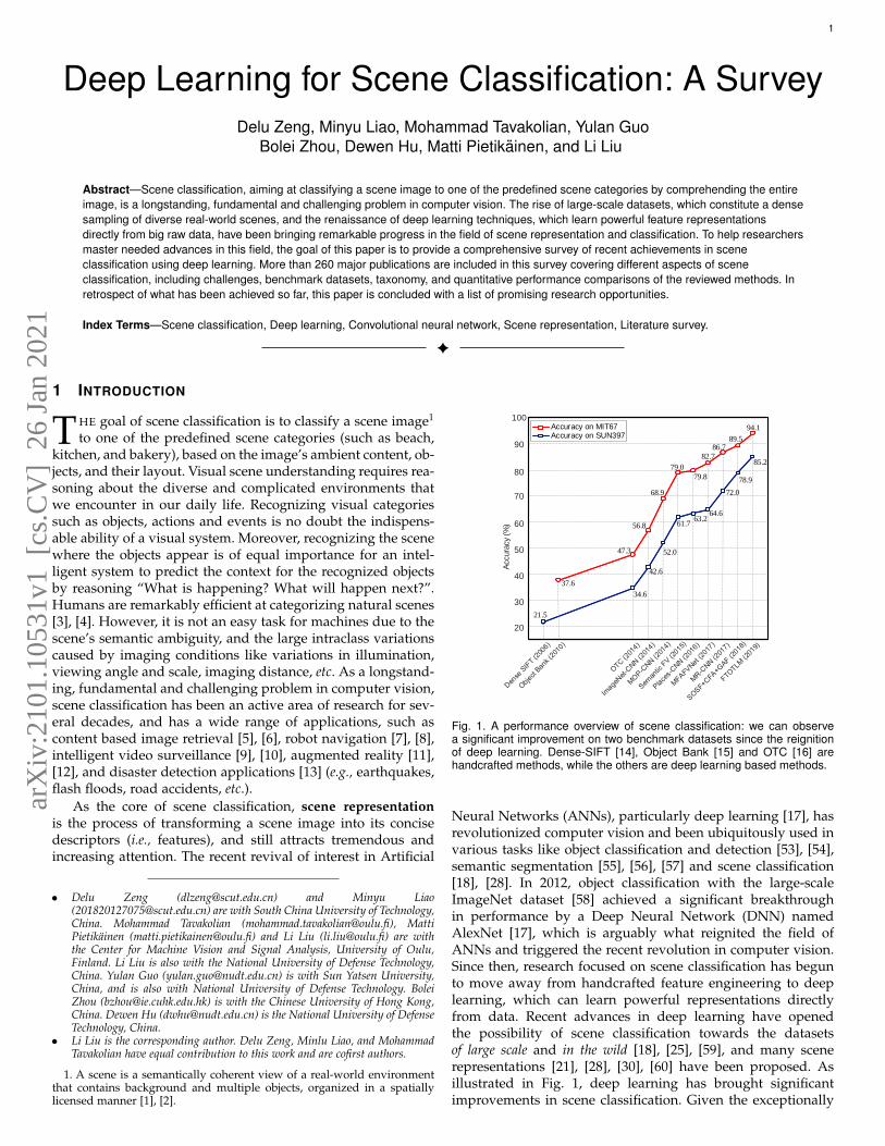
1

Deep Learning for Scene Classification: A SurveyDelu Zeng, Minyu Liao, Mohammad Tavakolian, Yulan Guo

Bolei Zhou, Dewen Hu, Matti Pietikainen, and Li Liu

Abstract—Scene classification, aiming at classifying a scene image to one of the predefined scene categories by comprehending the entireimage, is a longstanding, fundamental and challenging problem in computer vision. The rise of large-scale datasets, which constitute a densesampling of diverse real-world scenes, and the renaissance of deep learning techniques, which learn powerful feature representationsdirectly from big raw data, have been bringing remarkable progress in the field of scene representation and classification. To help researchersmaster needed advances in this field, the goal of this paper is to provide a comprehensive survey of recent achievements in sceneclassification using deep learning. More than 260 major publications are included in this survey covering different aspects of sceneclassification, including challenges, benchmark datasets, taxonomy, and quantitative performance comparisons of the reviewed methods. Inretrospect of what has been achieved so far, this paper is concluded with a list of promising research opportunities.

Index Terms—Scene classification, Deep learning, Convolutional neural network, Scene representation, Literature survey.

F

1 INTRODUCTION

THE goal of scene classification is to classify a scene image1

to one of the predefined scene categories (such as beach,kitchen, and bakery), based on the image’s ambient content, ob-jects, and their layout. Visual scene understanding requires rea-soning about the diverse and complicated environments thatwe encounter in our daily life. Recognizing visual categoriessuch as objects, actions and events is no doubt the indispens-able ability of a visual system. Moreover, recognizing the scenewhere the objects appear is of equal importance for an intel-ligent system to predict the context for the recognized objectsby reasoning “What is happening? What will happen next?”.Humans are remarkably efficient at categorizing natural scenes[3], [4]. However, it is not an easy task for machines due to thescene’s semantic ambiguity, and the large intraclass variationscaused by imaging conditions like variations in illumination,viewing angle and scale, imaging distance, etc. As a longstand-ing, fundamental and challenging problem in computer vision,scene classification has been an active area of research for sev-eral decades, and has a wide range of applications, such ascontent based image retrieval [5], [6], robot navigation [7], [8],intelligent video surveillance [9], [10], augmented reality [11],[12], and disaster detection applications [13] (e.g., earthquakes,flash floods, road accidents, etc.).

As the core of scene classification, scene representationis the process of transforming a scene image into its concisedescriptors (i.e., features), and still attracts tremendous andincreasing attention. The recent revival of interest in Artificial

• Delu Zeng (dlzeng@scut.edu.cn) and Minyu Liao(201820127075@scut.edu.cn) are with South China University of Technology,China. Mohammad Tavakolian (mohammad.tavakolian@oulu.fi), MattiPietikainen (matti.pietikainen@oulu.fi) and Li Liu (li.liu@oulu.fi) are withthe Center for Machine Vision and Signal Analysis, University of Oulu,Finland. Li Liu is also with the National University of Defense Technology,China. Yulan Guo (yulan.guo@nudt.edu.cn) is with Sun Yatsen University,China, and is also with National University of Defense Technology. BoleiZhou (bzhou@ie.cuhk.edu.hk) is with the Chinese University of Hong Kong,China. Dewen Hu (dwhu@nudt.edu.cn) is the National University of DefenseTechnology, China.

• Li Liu is the corresponding author. Delu Zeng, Minlu Liao, and MohammadTavakolian have equal contribution to this work and are cofirst authors.

1. A scene is a semantically coherent view of a real-world environmentthat contains background and multiple objects, organized in a spatiallylicensed manner [1], [2].

20

30

40

50

60

70

80

90

100

Accura

cy

(%)

37.6

47.3

56.8

68.9

79.0

79.8

82.7

86.789.5

94.1

21.5

34.6

42.6

52.0

61.763.2

64.6

78.9

85.2

72.0

Accuracy on MIT67Accuracy on SUN397

Fig. 1. A performance overview of scene classification: we can observea significant improvement on two benchmark datasets since the reignitionof deep learning. Dense-SIFT [14], Object Bank [15] and OTC [16] arehandcrafted methods, while the others are deep learning based methods.

Neural Networks (ANNs), particularly deep learning [17], hasrevolutionized computer vision and been ubiquitously used invarious tasks like object classification and detection [53], [54],semantic segmentation [55], [56], [57] and scene classification[18], [28]. In 2012, object classification with the large-scaleImageNet dataset [58] achieved a significant breakthroughin performance by a Deep Neural Network (DNN) namedAlexNet [17], which is arguably what reignited the field ofANNs and triggered the recent revolution in computer vision.Since then, research focused on scene classification has begunto move away from handcrafted feature engineering to deeplearning, which can learn powerful representations directlyfrom data. Recent advances in deep learning have openedthe possibility of scene classification towards the datasetsof large scale and in the wild [18], [25], [59], and many scenerepresentations [21], [28], [30], [60] have been proposed. Asillustrated in Fig. 1, deep learning has brought significantimprovements in scene classification. Given the exceptionally

arX

iv:2

101.

1053

1v1

[cs

.CV

] 2

6 Ja

n 20

21

2

Deep Learning based methods for Scene Classification (Section 4)Main CNN Framework (Section 4.1)

Pre-trained CNN Model: Object-centric CNNs [17], Scene-centric CNNs [18]Fine-tuned CNN Model: Scale-specific CNNs [19], DUCA [20], FTOTLM [21]Specific CNN Model: DL-CNN [22], GAP-CNN [23], CFA [24]

CNN based Scene Representation (Section 4.2)Global CNN Feature based Method: Places-CNN [18], [25], S2ICA [26], GAP-CNN [23], DL-CNN [22], HLSTM [27]Spatially Invariant Feature based Method: MOP-CNN [28], MPP-CNN [29], SFV [30], MFAFVNet [31], VSAD [32]Semantic Feature based Method: MetaObject-CNN [33], WELDON [34], SDO [35], M2M BiLSTM [36]Multi-layer Feature based Method: DAG [37], Hybrid CNNs [38], G-MS2F [39], FTOTLM [21]Multi-view Feature based Method: Scale-specific CNNs [19], LS-DHM [40], MR CNN [41]

Strategy for Improving Scene Representation (Section 4.3)Encoding Strategy: Semantic FV [30], FCV [40], VSAD [32], MFA-FS [42], MFAFVNet [31]Attention Strategy: GAP-CNN [23], MAPNet [43], MSN [44], LGN [45]Contextual Strategy: Correlation topic model [46], Sequential model [27], Graph-related model [45]Regularization Strategy: Sparse Regularization [22], Structured Regularization [44], Supervised Regularization [40]

RGB-D Scene Classification (Section 4.4)Depth-specific Feature Learning: Fine-tuning RGB-CNNs [47], Weak-supervised learning [48], Semi-supervised learning [49]Multiple Modality Fusion: Image-level modal fusion [50], Feature-level modal combination [51],

Consistent-feature based modal fusion [52], Distinctive-feature based modal fusion [44]

Fig. 2. A taxonomy of deep learning based methods for scene classification. With the rise of large-scale datasets, powerful feature representations aredirectly learned by using pre-trained CNNs, fine-tuned CNNs, or specific CNNs, having made remarkable progress. The representations mainly consistof global CNN features, spatially invariant features, semantic features, multi-layer features, and multi-view features. At the same time, the performancesof many methods are improved due to effective strategies, like orderless encoding, attention learning, context modeling, and regularization. In addition,methods using RGB-D datasets, as a new issue for scene classification, mainly focus on learning depth specific features, and fusing multi-modal features.

rapid rate of progress, this article attempts to track recentadvances and summarize their achievements to gain a clearerpicture of the current panorama in scene classification usingdeep learning.

Recently, several surveys for scene classification have alsobeen available, such as [61], [62], [63]. Cheng et al. [62] pro-vided a recent comprehensive review of the recent progress forremote sensing image scene classification. Wei et al. [61] carriedout an experimental study of 14 scene descriptors mainly inthe handcrafted feature engineering way for scene classifica-tion. Xie et al. [63] reviewed scene recognition approaches inthe past two decades, and most of discussed methods in theirsurvey appeared in this handcrafted way. As opposed to theseexisting reviews [61], [62], [63], this work herein summarizesthe striking success and dominance in indoor/outdoor sceneclassification using deep learning and its related methods, butnot including other scene classification tasks, e.g., remote sens-ing scene classification [62], [64], [65], acoustic scene classifi-cation [66], [67], place classification [68], [69], etc. The majorcontributions of this work can be summarized as follows:

• As far as we know, this paper is the first to specificallyfocus on deep learning methods for indoor/outdoor sceneclassification, including RGB scene classification, as wellas RGB-D scene classification.

• We present a taxonomy (see Fig. 2), covering the most re-cent and advanced progresses of deep learning for scenerepresentation.

• Comprehensive comparisons of existing methods onseveral public datasets are provided, meanwhile we alsopresent brief summaries and insightful discussions.

The remainder of this paper is organized as follows: Challengesand the related progress in scene classification made during thelast two decades are summarized in Section 2. The benchmarkdatasets are summarized in Section 3. In section 4, we presenta taxonomy of the existing deep learning based methods. Thenin section 5, we provide an overall discussion of their corre-sponding performance (Tables 2, 3, 5). Followed by Section 6we conclude important future research outlook.

2 BACKGROUND

2.1 The Problem and Challenge

Scene classification can be further dissected through analyzingits strong ties with related vision tasks such as objectclassification and texture classification. Scenes are usuallycomposed of multiple semantic parts, some of whichcorrespond to objects. And the texture information acrossscene categories is used to identify scenes [70]. As typicalpattern recognition problems, these tasks consist of featurerepresentation and classification. The strong ties between thesetasks have led to the fact that the division between scenerepresentation methods and object/texture representationmethods [71], [72] has been narrowing. However, in contrastto object classification (images are object-centric) or textureclassification (images include only textures), the observedscene images are more complicated, and further analysis areneeded by exploring the overall semantic content of scene, e.g.,what the semantic parts (e.g., objects, textures, background)are, in what way they are organized together, and what theirsemantic connections with each other are.

Human scene processing is characterized by its remarkableefficiency [3], [4]. Despite over several decades of developmentin scene classification, most of methods still have not beencapable of performing at a level sufficient for various real-world scenes. The inherent difficulty of scene classificationis due to the nature of complexity and high variance ofreal-world scenes. Overall, significant challenges in sceneclassification stem from large intraclass variations, semanticambiguity, and computational efficiency.

Large intraclass variation. Intraclass variation mainlyoriginates from intrinsic factors of the scene itself and imagingconditions. In terms of intrinsic factors, each scene can havemany different example images, possibly varying with largevariations among various objects, background, or humanactivities. Imaging conditions like changes in illumination,viewpoint, scale and heavy occlusion, clutter, shading, blur,motion, etc. contribute to large intraclass variations. Furtherchallenges may be added by digitization artifacts, noise

3

Semantic Ambiguity

Large Intraclass Variationshopping mall shopping mall shopping mall

library archive bookstore

Fig. 3. Scene exemplars of illustrating large intraclass variation andsemantic ambiguity. Top: The shopping malls are quite different with eachother caused by lighting conditions and overall content, which leads to largeintraclass variation. Below: General layout and uniformly arranged objectsare similar on archive, bookstore, and library, which leads to semanticambiguity.

corruption, poor resolution, and filtering distortion. Forinstance, three shopping malls (top row of Fig. 3) are shownwith different lighting conditions, viewing angle, and objects.

Semantic ambiguity. Since images of different classes mayshare similar objects, textures, background, etc., they look verysimilar in visual appearances, which causes ambiguity amongthem [73], [74]. The bottom row of Fig. 3 depicts strong visualcorrelation between three different indoor scenes, i.e., archive,bookstore, and library. With the emerging of new scene cat-egories, the problem of semantic ambiguity would be moreserious. In addition, scene category annotation is subjective,relying on the experience of the annotators, therefore a sceneimage may belong to multiple semantic categories [73], [75].

Computational efficiency. The prevalence of social medianetworks and mobile/wearable devices has led to increasingdemands for various computer vision tasks includingscene recognition. However, mobile/wearable devices haveconstrained computing related resources, making efficientscene recognition a pressing requirement.

2.2 A Road Map of Scene Classification in 20 yearsScene representation or scene feature extraction, the process ofconverting a scene image into feature vectors, plays the criticalrole in scene classification, and thus is the focus of researchin this field. In the past two decades, remarkable progress hasbeen witnessed in scene representation, which mainly consistsof two important generations: handcrafted feature engineering,and deep learning (feature learning). The milestones of sceneclassification in the past two decades are presented in Fig. 4, inwhich two main stages (SIFT vs. DNN) are highlighted.

Handcrafted feature engineering era. From 1995 to 2012,the field was dominated by the Bag of Visual Word (BoVW)model [80], [91], [92], [93], [94] borrowed from document clas-sification which represents a document as a vector of wordoccurrence counts over a global word vocabulary. In the imagedomain, BoVW firstly probes an image with local feature de-scriptors such as Scale Invariant Feature Transform (SIFT) [76],[95], and then represents an image statistically as an orderlesshistogram over a pre-trained visual vocabulary, in a similarform to a document. Some important variants of BoVW suchas Bag of Semantics [15], [84], [96], [97] and Improved FisherVector (IFV) [81], have also been proposed.

Local invariant feature descriptors play an importantrole in BoVW because they are discriminative, yet less

sensitive to image variations such as illumination, scale,rotation, viewpoint etc, and thus have been widely studied.Representative local descriptors for scene classification havestarted from SIFT [76], [95] and Global Information SystemsTechnology (GIST) [77], [98]. Other local descriptors, suchas Local Binary Patterns (LBP) [99], Deformable Part Model(DPM) [100], [101], [102], CENsus TRansform hISTogram(CENTRIST) [79], also contribute to the development ofscene classification. To improve the performance, researchfocus shifts to feature encoding and aggregation, mainlyincluding Bag-of-Visual-Words (BoVW) [92], Latent DirichletAllocation (LDA) [103], Histogram of Gradients (HoG) [78],Spatial Pyramid Matching (SPM) [14], [104], Vector ofLocally Aggregated Descriptors (VLAD) [82], Fisher kernelcoding [81], [105] and Orientational Pyramid Matching (OPM)[106]. The quality of the learned codebook has a great impacton the coding procedure. The generic codebooks mainlyinclude Fisher kernels [81], [105], sparse codebook [107], [108],Locality-constrained Linear Codes (LLC) [109], HistogramIntersection Kernels (HIK) [110], contextual visual words [111],Efficient Match Kernels (EMK) [112] and Supervised KernelDescriptors (SKDES) [113]. Particularly, semantic codebooksgenerate from salient regions, like Object Bank [15], [83], [114],object-to-class [115], Latent Pyramidal Regions (LPR) [116],Bags of Parts (BoP) [84] and Pairwise Constraints basedMultiview Subspace Learning (PC-MSL) [117], capturing morediscriminative features for scene classification.

Deep learning era. In 2012, Krizhevsky et al. [17]introduced a DNN, commonly referred to as “AlexNet”,for the object classification task, and achieved breakthroughperformance surpassing the best result of hand-engineeredfeatures by a large margin, and thus triggered the recentrevolution in AI. Since then, deep learning has started todominate various tasks (like computer vision [72], [118], [119],[120], speech recognition [121], autonomous driving [122],cancer detection [123], [124], machine translation [125],playing complex games [126], [127], [128], [129], earthquakeforecasting [130], medicine discovery [131], [132]), and sceneclassification is no exception, leading to a new generation ofscene representation methods with remarkable performanceimprovements. Such substantial progress can be mainlyattributed to advances in deep models including VGGNet [85],GoogLeNet [86], ResNet [87], etc., the availability of large-scaleimage datasets like ImageNet [58] and Places [18], [25] andmore powerful computational resources.

Deep learning networks have gradually replaced the localfeature descriptors of the first generation methods and arecertainly the engine for scene classification. Although the majordriving force of progress in scene classification has been theincorporation of deep learning networks, the general pipelineslike BoVW, feature encoding and aggregation methods likeFisher Vector, VLAD of the first generation methods havealso been adapted in current deep learning based scenemethods, e.g., MOP-CNN [28], SCFVC [133], MPP-CNN [29],DSP [134], Semantic FV [30], LatMoG [60], MFA-FS [42] andDUCA [20]. To take fully advantage of back-propagation,scene representations are extracted from end-to-end trainableCNNs, like DAG-CNN [37], MFAFVNet [31], VSAD [32],G-MS2F [39], and DL-CNN [22]. To focus on main content ofthe scene, object detection is used to capture salient regions,such as MetaObject-CNN [33], WELDON [34], SDO [35], andBiLSTM [36]. Since features from multiple CNN layers ormultiple views are complementary, many literatures [19], [21],

4

1999

SIFT: the most widely used local descriptor in computer vision (Lowe et al.)

GIST: a holistic representation of the scene spatial structure(Oliva et al.)

Bag of Visual Words: marking the beginning of BoVW in computer vision (Sivic et al.)

SPM: multilevel version of bag of words model to preserve spatial information(Lazebnik et al.)

ImageNet: a large-scale image dataset trigged the breakthrough of deep learning (Deng et al.)

SUN 397: the first large scale scene database (Xiao et al.)

Object Bank: models a scene as a response map of many generic object detectors (Li et al.)

AlexNet: the ConvNet that reignites the field of neural networks (Krizhevsky et al.)

Improved FV: a variant of BoW, encodes higher order statistics (Sanchez et al.)

Bags of Parts: learn distinctive parts of scenes automatically(Juneja et al.)

VGG: increases CNN depth with very small convolution filters (Simonyan et al.)

GoogLeNet: increases network depth with the parameter efficient inception module (Szegedy et al.)

MITPlaces: the largest scene database (Zhou et al.)

SUN RGB-D:A large RGB-D scene dataset (Song et al.)

MOP-CNN: first work to apply CNN for scene classification (Gong et al.)

GAP-CNN: highlighting the class-specific regions with global average pooling (Zhou et al.)

ResNet: revolution of network depth by using skip connections(He et al.)

2009 2010 2012

2006

2013 20142003 20162015

VLAD: simple and efficient version of Fisher Vector(Jegou et al.)

HoG: similar to SIFT, cells of dense gradient orientations(Dalal and Triggs)

2005 2011

CENTRIST: a local binary pattern like holistic representation method for scene (Wu et al.)

FV-CNN: combines CNN features and Fisher Vector(Cimpoi et al.)CNN “off the shelf”

(Razavian et al.)

Deep Learning Network

Feature Representation

Typical Dataset

2001

Semantic FV: develop Fisher vector on semantic features via natural parameterization(Dixit et al.)

Fig. 4. Milestones of scene classification. Handcrafted features gained tremendous popularity, starting from SIFT [76] and GIST [77]. Then, HoG [78] andCENTRIST [79] were proposed by Dalal et al. and Wu et al., respectively, further promoting the development of scene classification. In 2003, Sivic etal. [80] proposed BoVW model, marking the beginning of codebook learning. Along this way, more effective BoVW based methods, SPM [14], IFV [81] andVLAD [82], also emerged to deal with larger-scale tasks. In 2010, Object Bank [15], [83] represents the scene as object attributes, marking the beginningof more semantic representations. Then, Juneja et al. [84] proposed Bags of Part to learn distinctive parts of scenes automatically. In 2012, AlexNet [17]reignites the field of artificial neural networks. Since then, CNN-based methods, VGGNet [85], GoogLeNet [86] and ResNet [87], have begun to take overhandcrafted methods. Additionally, Razavian et al. [88] highlights the effectiveness and generality of CNN representations for different tasks. Along thisway, in 2014, Gong et al. [28] proposed MOP-CNN, the first deep learning methods for scene classification. Later, FV-CNN [89], Semantic FV [30] andGAP-CNN [23] are proposed one after another to learn more effective representations. For datasets, ImageNet [58] triggers the breakthrough of deeplearning. Then, Xiao et al. [59] proposed SUN database to evaluate numerous algorithms for scene classification. Later, Places [18], [25], the largest scenedatabase currently, emerged to satisfy the need of deep learning training. Additionally, SUN RGBD [90] has been introduced, marking the beginning ofdeep learning for RGB-D scene classification. See Section 2.2 for details.

[24], [40], [41] also explored their complementarity to improveperformance. In addition, there exists many strategies (likeattention mechanism, contextual modeling, multi-task learningwith regularization terms) to enhance representation ability,such as CFA [24], BiLSTM [36], MAPNet [43], MSN [44], andLGN [45]. For datasets, because depth images from RGB-Dcameras are not vulnerable to illumination changes, since 2015,researchers have started to explore RGB-D scene recognition.Some works [48], [49], [135] focus on depth-specific featurelearning, while other alternatives, like DMMF [52], ACM [136],and MSN [44] focus on multi-modal feature fusion.

3 DATASETS

This section reviews publicly available datasets for sceneclassification. The scene datasets (image examples are shownin Fig. 5) are broadly divided into two main categories basedon the image type: RGB and RGB-D datasets. The datasetscan further be divided into two categories in terms of theirsize. Small-size datasets (e.g., Scene15 [14], MIT67 [137],SUN397 [59], NYUD2 [138], SUN RGBD [90]) are usually usedfor evaluation, while large-scale datasets, e.g., ImageNet [58]and Places [18], [25], are essential for pre-training anddeveloping deep learning models. Table 1 summarizes thecharacteristics of these datasets for scene classification.

Scene15 dataset [14] is a small scene dataset containing4,448 grayscale images of 15 scene categories, i.e., 5 indoorscene classes (office, store, kitchen, bedroom, living room)along with 10 outdoor scene classes (suburb, forest, mountain,tall building, street, highway, coast, inside city, open country,industrial). Each class contains 210−410 scene images, and theimage size is around 300×250. The dataset is divided into twosplits; there are at least 100 images per class in the training set,and the rest are for testing.

MIT Indoor 67 (MIT67) dataset [137] covers a wide range ofindoor scenes, e.g., store, public space, and leisure. MIT67 com-

prises 15,620 scene images from 67 indoor categories, whereeach category has about 100 images. Moreover, all images havea minimum resolution of 200×200 pixels on the smallest axis.Because of the shared similarities among objects in this dataset,the classification of images is challenging. There are 80 and 20images per class in the training and testing set, respectively.

Scene UNderstanding 397 (SUN397) dataset [59] consistsof 397 scene categories, in which each category has more than100 images. The dataset contains 108,754 images with an im-age size of about 500×300 pixels. SUN397 spans over 175 in-door, 220 outdoor scene classes, and two classes with mixed in-door and outdoor images, e.g., a promenade deck with a ticketbooth. There are several train/test split settings with 50 imagesper category in the testing.

ImageNet dataset [58], derived from the Stanford Com-puter Vision Lab, is one of the most famous large-scale imagedatabases particularly used for visual tasks. It is organized interms of the WordNet [140] hierarchy, each node of which isdepicted by hundreds and thousands of images. Up to now,there are more than 14 million images and about 20 thousandnotes in the ImageNet. Usually, a subset of ImageNet dataset(about 1000 categories with a total of 1.2 million images [17])is used to pre-train the CNN for scene classification.

Places dataset [18], [25] is a large-scale scene dataset, whichprovides an exhaustive list of the classes of environments en-countered in the real world. The Places dataset has inheritedthe same list of scene categories from SUN397 [59]. As a result,it contains 7,076,580 images from 476 scene categories. Fourbenchmark subsets of Places are shown as follows:

• Places205 [18] has 2.5 million images from scenecategories. The image number per class varies from 5,000to 15,000. The training set has 2,448,873 images, with 100images per category for the validation set and 200 imagesper category for the testing set.

• Places88 [18] contains the 88 common scene categoriesamong the ImageNet [58], the SUN397 [59], and the

5

(a) Scene15 (b) MIT67 (c) SUN397 (d) ImageNet (e) Places (f) NYUD2 (g) SUN RGBD

RGB

Depth

HHA

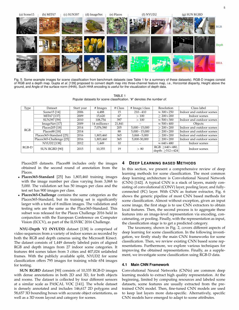
Fig. 5. Some example images for scene classification from benchmark datasets (see Table 1 for a summary of these datasets). RGB-D images consistof RGB and a depth map. Gupta et al. [139] proposed to convert depth map into three-channel feature map, i.e., Horizontal disparity, Height above theground, and Angle of the surface norm (HHA). Such HHA encoding is useful for the visualization of depth data.

TABLE 1Popular datasets for scene classification. “#” denotes the number of.

Type Dataset Start year # Images # Class # Image/class Resolution Class label

RGB

Scene15 [14] 2006 4,488 15 210−410 ≈ 300×250 Indoor and outdoor scenesMIT67 [137] 2009 15,620 67 > 100 ≥ 200×200 Indoor scenesSUN397 [59] 2010 108,754 397 > 100 ≈ 500×300 Indoor and outdoor scenes

ImageNet [17] 2009 14 millions+ 21,841 − ≈ 500×400 ObjectsPlaces205 [18] 2014 7,076,580 205 5,000−15,000 ≥ 200×200 Indoor and outdoor scenesPlaces88 [18] 2014 − 88 5,000−15,000 ≥ 200×200 Indoor and outdoor scenes

Places365-Standard [25] 2016 1,803,460 365 3,068−5,000 ≥ 200×200 Indoor and outdoor scenesPlaces365-Challenge [25] 2016 1,803,460 365 5,000-30,000 ≥ 200×200 Indoor and outdoor scenes

RGB-DNYUD2 [138] 2012 1,449 10 − ≈ 640×480 Indoor scenes

SUN RGBD [90] 2015 10,355 19 > 80 RGB: ≥640×480,depth: ≥512×424 Indoor scenes

Places205 datasets. Places88 includes only the imagesobtained in the second round of annotation from thePlaces.

• Places365-Standard [25] has 1,803,460 training imageswith the image number per class varying from 3,068 to5,000. The validation set has 50 images per class and thetest set has 900 images per class.

• Places365-Challenge contains the same categories as thePlaces365-Standard, but its training set is significantlylarger with a total of 8 million images. The validation andtesting sets are the same as the Place365-Standard. Thissubset was released for the Places Challenge 2016 held inconjunction with the European Conference on ComputerVision (ECCV), as part of the ILSVRC 2016 Challenge.

NYU-Depth V2 (NYUD2) dataset [138] is comprised ofvideo sequences from a variety of indoor scenes as recorded byboth the RGB and depth cameras using the Microsoft Kinect.The dataset consists of 1,449 densely labeled pairs of alignedRGB and depth images from 27 indoor scene categories. Itfeatures 464 scenes taken from 3 cities and 407,024 unlabeledframes. With the publicly available split, NYUD2 for sceneclassification offers 795 images for training while 654 imagesfor testing.

SUN RGBD dataset [90] consists of 10,335 RGB-D imageswith dense annotations in both 2D and 3D, for both objectsand rooms. The dataset is collected by four different sensorsat a similar scale as PASCAL VOC [141]. The whole datasetis densely annotated and includes 146,617 2D polygons and58,657 3D bounding boxes with accurate object orientations, aswell as a 3D room layout and category for scenes.

4 DEEP LEARNING BASED METHODS

In this section, we present a comprehensive review of deeplearning methods for scene classification. The most commondeep learning architecture is Convolutional Neural Network(CNN) [142]. A typical CNN is a stack of layers, mainly con-sisting of convolutional (CONV) layer, pooling layer, and fully-connected (FC) layer. With CNN as feature extractor, Fig. 6shows the generic pipeline of most CNN based methods forscene classification. Almost without exception, given an inputscene image, the first stage is to use CNN extractors to obtainlocal features. Then, the second process is to aggregate thesefeatures into an image-level representation via encoding, con-catenating, or pooling. Finally, with the representation as input,the classification stage is to get a predicted category.

The taxonomy, shown in Fig. 2, covers different aspects ofdeep learning for scene classification. In the following investi-gation, we firstly study the main CNN frameworks for sceneclassification. Then, we review existing CNN based scene rep-resentations. Furthermore, we explore various techniques forimproving the obtained representations. Finally, as a supple-ment, we investigate scene classification using RGB-D data.

4.1 Main CNN FrameworkConvolutional Neural Networks (CNNs) are common deeplearning models to extract high quality representation. At thebeginning, limited by computing resources and labeled scenedatasets, scene features are usually extracted from the pre-trained CNN model. Then, fine-tuned CNN models are usedto keep last layers more data-specific. Alternatively, specificCNN models have emerged to adapt to scene attributes.

6

Densesampling

...

...

...

...

N key patches

M

N

a×b

P

SVM

office

Scene Image

Feature Encoding and Pooling Category PredictionLocal Feature Extraction

RegionSampling

Single Pass

Sparse sampling

FeatureExtraction

Local Features

Global Representation

M patches

...

SelectedPatches

Feature Aggregation

Feature Classification

ab

P

Pooling (e.g. max pooling,global average pooling)

Multipass

Multipass Selecting key features

Concatenating

CategoryLabel

...

CNN

Conv.Layer

office

CNN

Encoding(e.g. VLAD, Fisher vector)

Softmax

Fig. 6. Generic pipeline of deep learning for scene classification. An entire pipeline consists of a module in each of the three stages (local feature extraction,feature encoding and pooling, and category prediction). The common pipelines are shown with arrows in different colors, including global CNN featurebased pipeline (blue arrows), spatially invariant feature based pipeline (green arrows), and semantic feature based pipeline (red arrows). Although thepipeline of some methods (like [31], [32]) are unified and trained in an end-to-end manner, they are virtually composed of these three stages.

4.1.1 Pre-trained CNN Model

The network architecture plays a pivotal role in the perfor-mance of deep models. In the beginning, AlexNet [17] servedas the mainstream CNN model for feature representation andclassification purposes. Later, Simonyan et al. [85] developedVGGNet and showed that, for a given receptive field, usingmultiple stacked small kernels is better than using a largeconvolution kernel, because applying non-linearity on multiplefeature maps yields more discriminative representations. Onthe other hand, the reduction of kernels receptive filed sizedecreases the number of parameters for bigger networks.Therefore, VGGNet has 3×3 convolution kernels insteadof large convolution kernels (i.e., 11×11, 7×7, and 5×5)in AlexNet. Motivated by the idea that only a handful ofneurons have an effective role in feature representation,Szegedy et al. [86] proposed an Inception module to makea sparse approximation of CNNs. Deeper the model, themore descriptive representations. This is the advantageof hierarchical feature extraction using CNN. However,constantly increasing CNNs depth could result in vanishingthe gradient through back-propagation of error from the lastFC layer to the input. To address this issue, He et al. [87]included skip connection to the hierarchical structure of CNNand proposed Residual Networks (ResNets). ResNets areeasier to optimize and can gain accuracy from considerablyincreased depth.

In addition to the network architecture, the performance ofCNN interwinds with a sufficiently large amount of trainingdata. However, the training data are scarce in certain applica-tions, which results in the under-fitting of the model during thetraining process. To overcome this issue, pre-trained modelscan be employed to effectively extract feature representationsof small datasets [118]. Training CNN on large-scale datasets,such as the ImageNet [58] and the Places [18], [25], makes themlearn enriched visual representations. Such models can furtherbe used as pre-trained models for other tasks. However, theeffectiveness of the employment of pre-trained models largelydepends on the similarity between the source and target do-mains. Yosinski et al. [143] documented that the transferabilityof pre-trained CNN models decreases as the similarity of the

target task and original source task decreases. Nevertheless,pre-trained models still have better performance than randominitialization of the models [143].

Pre-trained CNNs, as fixed feature extractors, are dividedinto two categories: object-centric and scene-centric CNNs.Object-centric CNNs refer to the model pre-trained on objectdatasets, e.g., the ImageNet [58], and deployed for sceneclassification. Since object images do not contain the diversityprovided by the scene [18], object-centric CNNs have limitedperformance for scene classification. Hence, scene-centricCNNs, pre-trained on scene images, like Places [18], [25], aremore effective to extract scene-related features.

Object-centric CNNs. Cimpoi et al. [89] asserted that thefeature representations obtained from object-centric CNNsare object descriptors since they have likely more objectdescriptive properties. The scene image is represented as abag of semantics [30], and object-centric CNNs are sensitive tothe overall shape of objects, so many methods [28], [30], [31],[89], [133] used object-centric CNNs to extract local featuresfrom different regions of the scene image. Another importantfactor in the effective deployment of object-centric CNNs isthe relational size of images in the source and target datasets.Although CNNs are generally robust against size and scale,the performance of object-centric CNNs is influenced byscaling because such models are originally pre-trained ondatasets to detect and/or recognize objects. Therefore, theshift to describing scenes, which have multiple objects withdifferent scales, would drastically affect their performance [19].For instance, if the image size of the target dataset is smallerthan the source dataset to a certain degree, the accuracy of themodel would be compromised.

Scene-centric CNNs. Zhou et al. [18], [25] demonstratedthe classification performance of scene-centric CNNs is betterthan object-centric CNNs since the former use the prior knowl-edge of the scene. Herranz et al. [19] found that Places-CNNsachieve better performance at larger scales; therefore, scene-centric CNNs generally extract the representations in the wholerange of scales [23]. Guo et al. [40] noticed that the CONV lay-ers of scene-centric CNNs capture more detail information ofa scene, such as local semantic regions and fine-scale objects,

7

which is crucial to discriminate the ambiguous scenes, whilethe feature representations obtained from the FC layers do notconvey such perceptive quality. Zhou et al. [144] showed thatscene-centric CNNs may also perform as object detectors with-out explicitly being trained on object datasets.

4.1.2 Fine-tuned CNN Model

Pre-trained CNNs, described in Section 4.1.1, perform as deepfeature extractor with prior knowledge of the image dataset,on which they are trained [6], [71]. However, using onlythe pre-training strategy would prevent exploiting the fullcapability of the deep models in describing the target scenesadaptively. Hence, fine-tuning the pre-trained CNNs using thetarget scene dataset improves their performance by reducingthe possible domain shift between two datasets [71]. Notably, asuitable weight initialization becomes very important, becauseit is quite difficult to train a deep network model with manyadjustable parameters and non-convex loss functions [145].Therefore, fine-tuning the pre-trained CNN contributes to theeffective training process [29], [30], [34], [146].

Fine-tuning a models parameters is a simple and effectivetechnique for transferring knowledge from a pre-trainedmodel. For CNNs, a common fine-tuning technique is thefreeze strategy. In this method, the last FC layer of a pre-trained model is replaced with a new FC layer with the samenumber of neurons as the classes in the target dataset (i.e.,MIT67, SUN397), while the previous CONV layers parametersare frozen, i.e., they are not updated during the fine-tuningprocess. Then, this modified CNN is fine-tuned by trainingon the target dataset. Herein, the back-propagation is stoppedafter the last FC layers, which allows these layers to learndiscriminative knowledges from the learned CONV layers.Through updating few parameters, training a complex modelusing small datasets would be affordable. Optionally, it is alsopossible to gradually unfreeze some layers to further enhancethe learning quality as the earlier layers would adapt newrepresentations from the target dataset. Alternatively, differentlearning rates could be assigned to different layers of CNN,in which the early layers of the model have very low learningrate and the last layers have higher learning rates. In this way,the early CONV layers that have more abstract representationsare less affected, while the specialized FC layers are fine-tunedwith higher speed.

The size of the target dataset is an important factor forthe fine-tuning process. Deep models may not benefit fromfine-tuning on a small target dataset [71]. In this case, fine-tuning has negative effects since the structure of specializedFC layers has changed while inadequate training data areprovided for fine-tuning. Data augmentation is one alternativeto deal with the small size of the target dataset [20], [21], [49],[147]. Khan et al. [20] augmented the scene image dataset withflipped, cropped, and rotated versions to increase the size ofthe dataset and further improve the robustness of the learnedrepresentations. Liu et al. [21] used a sliding cropping windowto generate new patches from an image and selected thosepatches with sufficiently enough representative information ofthe original image.

There exists a problem via data augmentation to fine-tuneCNNs for scene classification. Herranz et al. [19] asserted thatfine-tuning a CNN model have certain “equalizing” effect be-tween the input patch scale and final accuracy, i.e., to someextent, with too small patches as CNN inputs, the final clas-sification accuracy is worse. This is because the small patch

inputs only contain part of image information, while the fi-nal labels indicate scene categories. Moreover, the number ofcropped patches is huge, so just a tiny part of these patchesis used to fine-tune CNN models, rendering limited overallimprovement [19]. On the other hand, Herranz et al. [19] alsoexplored the effect of fine-tuning CNNs on different scales, i.e.,with different scale patches as inputs. From the practical re-sults, there is a moderate accuracy gain in the range of scalepatches where the original CNNs perform poorly, e.g., in thecases of global scales for ImageNet-CNN and local scales forPlaces-CNN. However, there is marginal or no gain in rangeswhere CNN have already strong performance. For example,since Places-CNN has the best performance in the whole rangeof scale patches, in this case, fine-tuning on target dataset leadsto negligible performance improvement.

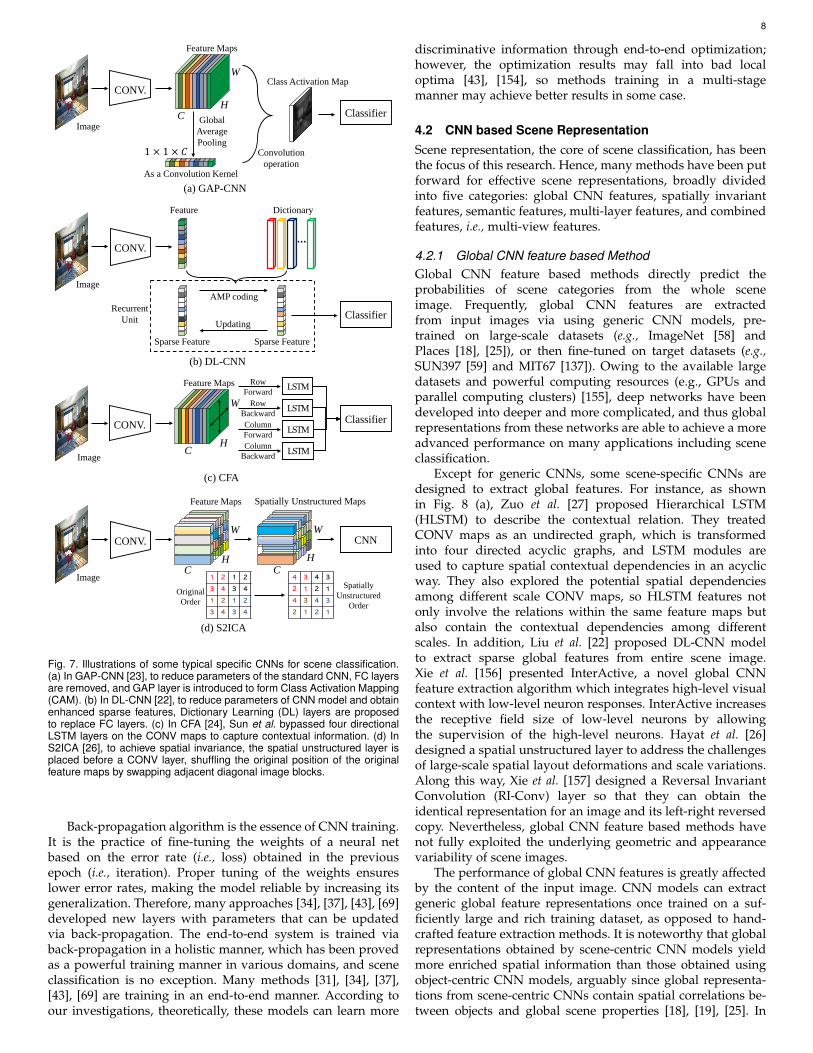
4.1.3 Specific CNN ModelIn addition to the generic CNN models, i.e., pre-trained CNNmodels and the fine-tuned CNN models, another group ofdeep models are specifically designed for scene classification.These models are specifically developed to extract effectivescene representations from the input by introducing newnetwork architectures. As is shown in Fig. 7, we only showfour typical specific models [22], [23], [24], [26].

To capture discriminative information from regions of in-terest, Zhou et al. [23] replaced the FC layers in a CNN modelwith a Global Average Pooling (GAP) layer [148] followed bya Softmax layer, i.e., GAP-CNN. As shown in Fig. 7 (a), by asimple combination of the original GAP layer and the 1×1 con-volution operation to form a class activation map (CAM), GAP-CNN can focus on class-specific regions and perform sceneclassification well. Although the GAP layer has a lower numberof parameters than the FC layer [23], [49], the GAP-CNN canobtain comparable classification accuracy.

Hypothesizing that a certain amount of sparsity improvesthe discriminability of the feature representations [149], [150],[151], Liu et al. [22] proposed a sparsity model named Dictio-nary Learning CNN (DL-CNN), seen in Fig. 7 (b). They re-placed FC layers with new dictionary learning layers, whichare composed of a finite number of recurrent units that corre-spond to iteration processes in the Approximate Message Pass-ing [152]. In particular, these dictionary learning layers param-eters are updated through back-propagation in an end-to-endmanner.

Since the CONV layers perform local operations on smallpatches of the image, they are not able to explicitly describethe contextual relation between different regions of the sceneimage. To address this limitation, Sun et al. [24] proposed Con-textual features in Appearance (CFA) based on LSTM [153]. Asshown in Fig. 7 (c), CONV feature maps are regarded as theinput of LSTM layers, which is transformed into four directedsequences in an acyclic way. Finally, LSTM layers are used todescribe spatial contextual dependencies, and the output offour LSTM modules are concatenated to describe contextualrelations in appearance.

Sequential operations of CONV and FC layers in standardCNNs retain the global spatial structure of the image, whichshows global features are sensitive to geometrical variations[28], [43], e.g., object translations and rotation directly affect theobtained deep features, which drastically limits the applicationof these features for scene classification. To achieve geometricinvariance, as shown in Fig. 7 (d), Hayat et al. [26] designed aspatial unstructured layer to introduce robustness against spa-tial layout deformations.

8

Spatially Unstructured MapsFeature Maps

CH

WCONV. CNN

ImageC

H

W

Feature Maps

Class Activation Map

Global AveragePooling

C

1 × 1 × 𝐶𝐶

H

W

CONV.

As a Convolution Kernel

Convolutionoperation

ClassifierImage

Feature

…

Dictionary

Sparse Feature

AMP codingRecurrent

Unit UpdatingClassifier

Sparse Feature

CONV.

Image

(a) GAP-CNN

(b) DL-CNN

(d) S2ICA

4 3 4 3

2 1 2 1

4 3 4 3

2 1 2 1

1 2 1 2

3 4 3 4

1 2 1 2

3 4 3 4

Original Order

SpatiallyUnstructured

Order

CONV.

Image

LSTM

LSTM

LSTM

LSTM

Feature Maps

CH

W

Row Forward

Row Backward Column Forward Column

Backward

Classifier

(c) CFA

Fig. 7. Illustrations of some typical specific CNNs for scene classification.(a) In GAP-CNN [23], to reduce parameters of the standard CNN, FC layersare removed, and GAP layer is introduced to form Class Activation Mapping(CAM). (b) In DL-CNN [22], to reduce parameters of CNN model and obtainenhanced sparse features, Dictionary Learning (DL) layers are proposedto replace FC layers. (c) In CFA [24], Sun et al. bypassed four directionalLSTM layers on the CONV maps to capture contextual information. (d) InS2ICA [26], to achieve spatial invariance, the spatial unstructured layer isplaced before a CONV layer, shuffling the original position of the originalfeature maps by swapping adjacent diagonal image blocks.

Back-propagation algorithm is the essence of CNN training.It is the practice of fine-tuning the weights of a neural netbased on the error rate (i.e., loss) obtained in the previousepoch (i.e., iteration). Proper tuning of the weights ensureslower error rates, making the model reliable by increasing itsgeneralization. Therefore, many approaches [34], [37], [43], [69]developed new layers with parameters that can be updatedvia back-propagation. The end-to-end system is trained viaback-propagation in a holistic manner, which has been provedas a powerful training manner in various domains, and sceneclassification is no exception. Many methods [31], [34], [37],[43], [69] are training in an end-to-end manner. According toour investigations, theoretically, these models can learn more

discriminative information through end-to-end optimization;however, the optimization results may fall into bad localoptima [43], [154], so methods training in a multi-stagemanner may achieve better results in some case.

4.2 CNN based Scene RepresentationScene representation, the core of scene classification, has beenthe focus of this research. Hence, many methods have been putforward for effective scene representations, broadly dividedinto five categories: global CNN features, spatially invariantfeatures, semantic features, multi-layer features, and combinedfeatures, i.e., multi-view features.

4.2.1 Global CNN feature based MethodGlobal CNN feature based methods directly predict theprobabilities of scene categories from the whole sceneimage. Frequently, global CNN features are extractedfrom input images via using generic CNN models, pre-trained on large-scale datasets (e.g., ImageNet [58] andPlaces [18], [25]), or then fine-tuned on target datasets (e.g.,SUN397 [59] and MIT67 [137]). Owing to the available largedatasets and powerful computing resources (e.g., GPUs andparallel computing clusters) [155], deep networks have beendeveloped into deeper and more complicated, and thus globalrepresentations from these networks are able to achieve a moreadvanced performance on many applications including sceneclassification.

Except for generic CNNs, some scene-specific CNNs aredesigned to extract global features. For instance, as shownin Fig. 8 (a), Zuo et al. [27] proposed Hierarchical LSTM(HLSTM) to describe the contextual relation. They treatedCONV maps as an undirected graph, which is transformedinto four directed acyclic graphs, and LSTM modules areused to capture spatial contextual dependencies in an acyclicway. They also explored the potential spatial dependenciesamong different scale CONV maps, so HLSTM features notonly involve the relations within the same feature maps butalso contain the contextual dependencies among differentscales. In addition, Liu et al. [22] proposed DL-CNN modelto extract sparse global features from entire scene image.Xie et al. [156] presented InterActive, a novel global CNNfeature extraction algorithm which integrates high-level visualcontext with low-level neuron responses. InterActive increasesthe receptive field size of low-level neurons by allowingthe supervision of the high-level neurons. Hayat et al. [26]designed a spatial unstructured layer to address the challengesof large-scale spatial layout deformations and scale variations.Along this way, Xie et al. [157] designed a Reversal InvariantConvolution (RI-Conv) layer so that they can obtain theidentical representation for an image and its left-right reversedcopy. Nevertheless, global CNN feature based methods havenot fully exploited the underlying geometric and appearancevariability of scene images.

The performance of global CNN features is greatly affectedby the content of the input image. CNN models can extractgeneric global feature representations once trained on a suf-ficiently large and rich training dataset, as opposed to hand-crafted feature extraction methods. It is noteworthy that globalrepresentations obtained by scene-centric CNN models yieldmore enriched spatial information than those obtained usingobject-centric CNN models, arguably since global representa-tions from scene-centric CNNs contain spatial correlations be-tween objects and global scene properties [18], [19], [25]. In

9

(a) HLSTM (b) SFV (c) WELDON (d) FTOTLM (e) Scale-specific network

Semantic Fisher Vector

(SFV)

NaturalParameterization

Fisher Vector

GMM Scene CNN

Object CNN

PoolingPooling

CConcatenate

Object CNN

Residual Block

Residual Block

Residual Block

Conv.

Batch Normalization+ ReLu + GAP

CNN

Weakly-Supervised Prediction

(WSP)

𝟏𝟏×𝟏𝟏CONV

Min layer

Max layer

CSFV WSP

… … ……

… …

…

Feature Concatenation

. . .

. . .Conv.

Conv.

Conv.

Conv.

SpatialLSTM layer

(SLSTM)

LSTM

LSTM

LSTM

LSTM

Feat

ure C

onca

tena

tion

Conv. map

CONVlayers

SLSTM

Image Dense Patches Regions Image Coarse Patches Fine PatchesYellow:negativeRed: positive

SLSTM . . .

Different Scales

Fig. 8. Five typical architectures to extract CNN based scene representations (see Section 4.2), respectively. Hourglass architectures are backbonenetworks, such as AlexNet or VGGNet. (a) HLSTM [27], a global CNN feature based method, extracts deep feature from the whole image. Spatial LSTMis used to model 2D characteristics among the spatial layout of image regions. Moreover, Zuo et al. captured cross-scale contextual dependencies viamultiple LSTM layers. (b) SFV [30], a spatially invariant feature based method, extract local features from dense patches. The highlight of SFV is toadd a natural parameterization to transform the semantic space into a natural parameter space. (c) WELDON [34], a semantic feature based method,extracts deep features from top evidence (red) and negative instances (yellow). In WSP scheme, Durand et al. used the max layer and min layer toselect positive and negative instances, respectively. (d) FTOTLM [21], a typical multi-layer feature based method, extracts deep feature from each residualblock. (e) Scale-specific network [19], a multi-view feature based architecture, used scene-centric CNN extract deep features from coarse versions, whileobject-centric CNN is used to extract features from fine patches. Two types of deep features complement each other.

addition, Herranz et al. [19] showed that the performance of ascene recognition system depends on the entities in the sceneimage, i.e., when the global features are extracted from imageswith chaotic background, the models performance is degradedcompared to the cases that the object is isolated from the back-ground or the image has a plain background. This suggests thatthe background may introduce some noise into the feature thatweakens the performance. Since contour symmetry provides aperceptual advantage when human observers recognize com-plex real-world scenes, Rezanejad et al. [158] studied globalCNN features from the full image and only contour informa-tion and showed that the performance of the full image asinput is better, because CNN captures potential informationfrom images. Nevertheless, they still concluded that contour isan auxiliary clue to improve recognition accuracy.

4.2.2 Spatially Invariant Feature based MethodTo alleviate the problems caused by sequential operationsin the standard CNN, a body of alternatives [28], [40],[89] proposed spatially invariant feature based methods tomaintain spatial robustness. The “spatially invariant” meansthat the output features are robust against the geometricalvariations of the input image [43].

As shown in Fig. 8 (b), spatially invariant features are usu-ally extracted from multiple local patches. The visualization ofsuch a feature extraction process is shown in Fig. 6 (markedin green arrows). The entire process can be decomposed intofive basic steps: 1) Local patch extraction: a given input imageis divided into smaller local patches, which are used as theinput to a CNN model, 2) Local feature extraction: deep fea-tures are extracted from either the CONV or FC layers of themodel, 3) Codebook generation: this step is to generate a code-book with multiple codewords based on the extracted deepfeatures from different regions of the image. The codewordsusually are learned in an unsupervised way (e.g., using GMM),4) Spatially invariant feature generation: given the generatedcodebook, deep features are encoded into a spatially invari-ant representation, and 5) Class prediction: the representationinput is classified into a predefined scene category.

As opposed to patch-based local feature extraction (each lo-cal feature is extracted from an original patch by independently

using the CNN extractor), local features can also be extractedfrom the semantic CONV maps of a standard CNN [29], [44],[134], [159]. Specifically, since each cell (deep descriptor) of thefeature map corresponds to one local image patch in the inputimage, each cell is regarded as a local feature. In this approach,the computation time is decreased, compared to independentlyprocessing of multiple spatial patches to obtain local features.For instance, Yoo et al. [29] replaced the FC layers with CONVlayers to obtain large amount of local spatial features. Theyalso used multi-scale CNN activations to achieve geometricrobustness. Gao et al. [134] used a spatial pyramid to directlydivide the activations into multi-level pyramids, which containmore discriminative spatial information.

The feature encoding technique, which aggregates the lo-cal features, is crucial in relating local features with the finalfeature representation, and it directly influences the accuracyand efficiency of the scene classification algorithms [71]. Im-proved Fisher Vector (IFV) [81], Vector of Locally AggregatedDescriptors (VLAD) [82], and Bag-of-Visual-Word (BoVW) [92]are among the popular and effective encoding techniques thatare used in deep learning based methods. For instance, manymethods, like FV-CNN [89], MFA-FS [42], and MFAFVNet [31],apply IFV encoding to obtain the image embedding as spatiallyinvariant representations, while MOP-CNN [28], SDO [35], etcutilize VLAD to cluster local features. Noteworthily, the code-book selection and encoding procedures result in disjoint train-ing of the model. To this end, some works proposed networksthat are trained in an end-to-end manner, e.g., NetVLAD [69],MFAFVNet [31], and VSAD [32].

Spatially invariant feature based methods are efficientto achieve geometric robustness. Nevertheless, the slidingwindows based paradigm requires multi-resolution scanningwith fixed aspect ratios, which is not suitable for arbitraryobjects with variable sizes or aspect ratios in the scene image.Moreover, using dense patches may introduce noise intothe final representation, which decreases the classificationaccuracy. Therefore, extracting semantic features from salientregions of the scene image can circumvent these drawbacks.

10

4.2.3 Semantic Feature based MethodProcessing all patches of the input image requires computa-tional cost while yields redundant information. Object detec-tion determines whether or not any instance of the salient re-gions is presented in an image [72]. Inspired by this, object de-tector based approaches allow identifying salient regions of thescene, which provide distinctive information about the contextof the image.

Different methods have been put forward to effectivesaliency detection, such as selective search [160], unsuper-vised discovery [161], Multi-scale Combinatorial Grouping(MCG) [162], and object detection networks (e.g., FastRCNN [53], Faster RCNN [54], SSD [163], Yolo [164], [165]).For instance, since selective search combines the strengthsof exhaustive search and segmentation, Liu et al. [146] usedit to capture all possible semantic regions, and then used apre-trained CNN to extract the feature maps of each regionfollowed by a spatial pyramid to reduce map dimensions.Because the common objects or characteristics in differentscenes lead to the commonality of different scenes, Cheng etal. [35] used a region proposal network [54] to extract thediscriminative regions while discarde non-discriminativeregions. These semantic feature based methods [35], [146]harvest many semantic regions, so encoding technology isadapted to aggregate key features, which pipeline is shown inFig. 6 (red arrows).

On the other hand, some semantic feature based meth-ods [33], [34] are based on weakly supervised learning, whichdirectly predicts categories by several semantic features ofthe scene. For instance, Wu et al. [33] generated high-qualityproposal regions by using MCG [162], and then used SVMon each scene category to prune outliers and redundantregions. Semantic features from different scale patches supplycomplementary cues, since the coarser scales deal with largerobjects, while the finer levels provide smaller objects orobject parts. In practice, they found two semantic featuressufficient to represent the whole scene, comparable to multiplesemantic features. Training a deep model only using asingle salient region may result in a suboptimal performancedue to the possible existence of outliers in the training set.Hence, multiple regions can be selected to train the modeltogether [34]. As shown in Fig. 8 (c), Durand et al. [34]designed a Max layer to select the attention regions to enhancethe discrimination. To provide a more robust strategy, theyalso designed a Min layer to capture the regions with the mostnegative evidence to further improve the model.

Although better performance can be obtained via usingmore semantic local features, semantic feature based methodsdeeply rely on the performance of object detection. Weaksupervision settings (i.e., without the patch labels of sceneimages) make it difficult to accurately identify the scene bythe key information of an image [34]. Moreover, the erroraccumulation problem and extra computation cost also limitthe development of semantic feature based methods [159].

4.2.4 Multi-layer Feature based MethodGlobal feature based methods usually extract the high-layerCNN features, and feed them into a classifier to achieve clas-sification task. Due to the compactness of such high-layer fea-tures, it is easy to miss some important slight clues [40], [166].Features from different layers are complementary [33], [167].Low-layer features generally capture small objects, while high-layer features capture big objects [33]. Moreover, semantic in-

formation of low-layer features is relatively less, but the objectlocation is accurate [167]. To take full advantage of featuresfrom different layers, many methods [21], [38], [39], [48] usedthe high resolution features from the early layers along withthe high semantic information of the features from the latestlayers of hierarchical models (e.g., CNNs).

As shown in Fig. 8 (d), typical multi-layer feature forma-tion process includes: 1) Feature extraction: the outputs (fea-ture maps) of certain layers are extracted as deep features, 2)Feature vectorization: vectorize the extracted feature maps, 3)Multi-layer feature combination: multiple features from differ-ent layers are combined into a single feature vector, and 4)Feature classification: classify the given scene image based onthe obtained combined feature.

Although using all features from different layers seems toimprove the final representation, it likely increases the chanceof overfitting, and thus hurts performance [37]. Therefore,many methods [21], [37], [38], [39], [48] only extract featuresfrom certain layers. For instance, Xie et al. [38] constructed twodictionary-based representations, Convolution Fisher Vector(CFV), and Mid-level Local Discriminative Representation(MLR) to classify subsidiarily scene images. Tang et al. [39]divided GoogLeNet layers into three parts from bottom totop and extracted final feature maps of each part. Liu etal. [21] captured feature maps from each residual block fromResNet independently. Song et al. [48] selected discriminativecombinations from different layers and different networkbranches via minimizing a weighted sum of the probability oferror and the average correlation coefficient. Yang et al. [37]used greedily select to explore the best layer combinations.

Feature fusion in multi-layer feature based methods isanother important direction. Feature fusion techniques aremainly divided into two groups [168], [169], [170]: 1) Earlyfusion: extracting multi-layer features and merging theminto a comprehensive feature for scene classification, and 2)Late fusion: directly learning each multi-layer feature via asupervised learner, which enforces the features to be directlysensitive to the category label, and then merging them intoa final feature. Although the performance of late fusion isbetter, it is more complex and time-consuming, so early fusionis more popular [21], [38], [39], [48]. In addition, additionand product rules are usually applied to combine multiplefeatures [39]. Since the feature spaces in different layers aredisparate, product rule is better than addition rule to fusingfeatures, and empirical experiments on [39] also show thisstatement. Moreover, Tang et al. [39] proposed two strategiesto fuse multi-layer features, i.e., ‘fusion with score’ and ‘fusionwith features’. Fusion with score technique has obtained abetter performance over fusion with feature thanks to theend-to-end training.

4.2.5 Multiple-view Feature based MethodDescribing a complex scene using just a single and compactfeature representation is a non-trivial task. Hence, there hasbeen a lot of effort to compute a comprehensive representa-tion of a scene by integrating multiple features obtained fromcomplementary CNN models [24], [32], [41], [171], [172], [173].

Feature, from the networks trained on different datasets,usually are complementary. As shown in Fig. 8 (e), Herranz etal. [19] found the best scale response of object-centric CNNsand scene-centric CNNs, and they combine the knowledge ina scale-adaptive way via either object-centric CNNs or scene-centric CNNs. Along this way, Wang et al. [173] used an object-centric CNN to carry information about object depicted in the

11

image, while a scene-centric CNN was used to capture globalscene information. The authors in [32] designed PatchNet, aweakly supervised learning method, which uses image-levelsupervision information as the supervision signal for effectiveextraction of the patch-level features. To enhance the recogni-tion performance, Scene-PatchNet and Object-PatchNet jointlyused to extract features for each patch.

Employing the complementary CNN architectures isessential for obtaining discriminative multi-view featurerepresentations. Wang et al. [41] proposed a multi-resolutionCNN (MR-CNN) architecture to capture visual content in mul-tiple scale images. In their work, normal BN-Inception [174]is used to extract coarse resolution features, while deeperBN-Inception is employed to extract fine resolution features.Jin et al. [175] used global features and spatially invariantfeatures to account for both the coarse layout of the scene andthe transient objects. Sun et al. [24] separately extracted threerepresentations, i.e., object semantics representation, contextualinformation, and global appearance, from discriminativeviews, which are complementarity to each other. Specifically,the object semantic features of the scene image are extractedby a CNN followed by spatial fisher vectors, while the deepfeature of a multi-direction LSTM-based model representscontextual information, and the FC feature represents globalappearance. Li et al. [171] used off-the-shelf ResNet18 [87]to generate discriminative attention maps, which is used asan explicit input of CNN together with the original image.Using global features extracted by ResNet-18 and attentionmap features extracted from the spatial feature transformernetwork, the attention map features are multiplied to theglobal features for adaptive feature refinement so that thenetwork focuses on the most discriminative parts.

4.3 Strategies for Improving Scene RepresentationTo obtain more discriminative representations for scene classi-fication, a range of strategies has been proposed. Four majorcategories (i.e., encoding strategy, attention strategy, contextualstrategy, and regularization strategy) will be discussed below.

4.3.1 Encoding strategyAlthough the current driving force has been the incorporationof CNNs, encoding technology of the first generation methodshave also been adapted in deep learning based methods.Fisher Vector (FV) coding [81], [105] is an encoding techniquecommonly used in scene classification. Fisher vector stores themean and the covariance deviation vectors per componentof the GMM and each element of the local features together.Thanks to the covariance deviation vectors, FV encoding leadsto excellent results. Moreover, it is empirically proven thatFisher vectors are complementary to global CNN features [30],[31], [38], [40], [42], [47]. Therefore, this survey takes FV-basedapproaches as the major cue and discusses the adaptedcombination of encoding technology and deep learning.

Generally, CONV features and FC features are regardedas Bags of Features (BoF), they can be readily modeledby the Gaussian Mixture Model followed by Fisher Vector(GMM-FV) [30], [31]. To avoid the computation of the FClayers, Cimpoi et al. [89] utilized GMM-FV to aggregateBoF from different CONV layers, respectively. Comparingtheir experiment results, they asserted that the last CONVfeatures can more effectively represent scenes. To rescue thefine-grained information of early/middle layers, Guo et al. [40]proposed Fisher Convolutional Vector (FCV) to encode the

(d) VSAD

(b) Semantic FV

(c) MFA-FV layer

(a) Basic FV

BoS features

(𝜋𝜋, 𝜇𝜇,𝛴𝛴 ) (𝜈𝜈, 𝜇𝜇,𝛴𝛴 )

GMM

Naturalparametrization

FVBoF features

(𝜋𝜋, 𝜇𝜇,𝛴𝛴 )GMM

FV

BoS features

(𝜇𝜇,𝑃𝑃,𝛬𝛬,𝛺𝛺, 𝑙𝑙𝑙𝑙𝑙𝑙 𝑘𝑘)

FV

MFA

BoF

BoS

features(𝜋𝜋, 𝜇𝜇,𝛴𝛴)

Softmax

Codebookconstruction

FV

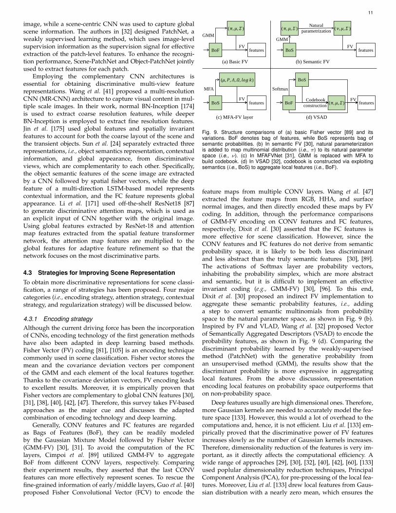
Fig. 9. Structure comparisons of (a) basic Fisher vector [89] and itsvariations. BoF denotes bag of features, while BoS represents bag ofsemantic probabilities. (b) In semantic FV [30], natural parameterizationis added to map multinomial distribution (i.e., π) to its natural parameterspace (i.e., ν). (c) In MFAFVNet [31], GMM is replaced with MFA tobuild codebook. (d) In VSAD [32], codebook is constructed via exploitingsemantics (i.e., BoS) to aggregate local features (i.e., BoF).

feature maps from multiple CONV layers. Wang et al. [47]extracted the feature maps from RGB, HHA, and surfacenormal images, and then directly encoded these maps by FVcoding. In addition, through the performance comparisonsof GMM-FV encoding on CONV features and FC features,respectively, Dixit et al. [30] asserted that the FC features ismore effective for scene classification. However, since theCONV features and FC features do not derive from semanticprobability space, it is likely to be both less discriminantand less abstract than the truly semantic features [30], [89].The activations of Softmax layer are probability vectors,inhabiting the probability simplex, which are more abstractand semantic, but it is difficult to implement an effectiveinvariant coding (e.g., GMM-FV) [30], [96]. To this end,Dixit et al. [30] proposed an indirect FV implementation toaggregate these semantic probability features, i.e., addinga step to convert semantic multinomials from probabilityspace to the natural parameter space, as shown in Fig. 9 (b).Inspired by FV and VLAD, Wang et al. [32] proposed Vectorof Semantically Aggregated Descriptors (VSAD) to encode theprobability features, as shown in Fig. 9 (d). Comparing thediscriminant probability learned by the weakly-supervisedmethod (PatchNet) with the generative probability froman unsupervised method (GMM), the results show that thediscriminant probability is more expressive in aggregatinglocal features. From the above discussion, representationencoding local features on probability space outperforms thaton non-probability space.

Deep features usually are high dimensional ones. Therefore,more Gaussian kernels are needed to accurately model the fea-ture space [133]. However, this would a lot of overhead to thecomputations and, hence, it is not efficient. Liu et al. [133] em-pirically proved that the discriminative power of FV featuresincreases slowly as the number of Gaussian kernels increases.Therefore, dimensionality reduction of the features is very im-portant, as it directly affects the computational efficiency. Awide range of approaches [29], [30], [32], [40], [42], [60], [133]used poplular dimensionality reduction techniques, PrincipalComponent Analysis (PCA), for pre-processing of the local fea-tures. Moreover, Liu et al. [133] drew local features from Gaus-sian distribution with a nearly zero mean, which ensures the

12

sparsity of the resulting FV. Wang et al. [47] enforced intercom-ponent sparsity of GMM-FV features via component regular-ization to discount unnecessary components.

Due to the non-linear property of deep features and a lim-ited ability of the covariance of GMM, a large number of di-agonal GMM components are required to model deep featuresso that the FV has very high dimensions [31], [42]. To addressthis issue, Dixit et al. [42] proposed MFA-FS, in which GMM isreplaced by Mixtures of Factor Analysis (MFA) [176], [177], i.e.,a set of local linear subspaces is used to capture non-linear fea-tures. MFA-FS performs well but does not support end-to-endtraining. However, end-to-end training is more efficient thanany disjoint training process [31]. Therefore, Li et al. [31] pro-posed MFAFVnet, an improved variant of MFA-FS [42], whichis conveniently embedded into the state-of-the-art network ar-chitectures. Fig. 9 (c) shows the MFA-FV layer of MFAFVNet,compared with the other two structures.

In FV coding, local features are assumed to be independentand identically distributed (iid), which violates intrinsic imageattributes that these patches are not iid. To this end, Cinbis etal. [60] introduced a non-iid model via treating the model pa-rameters as latent variables, rendering features related locally.Later, Wei et al. [46] proposed a correlated topic vector, treatedas an evolution oriented from Fisher kernel framework, to ex-plore latent semantics, and consider semantic correlation.

4.3.2 Attention strategyAs opposed to semantic feature based methods, focusing onkey cues generally from original images, attention policy aimsto select distinguishing features from the extracted featurespace [43], [44], [74], [178]. The attention maps are learnedwithout any explicit training signal, rather task-related lossfunction alone provides the training signal for the attentionweights. Noteworthily, GAP-CNN [23] is a simple attentionmethod, widely used in many works [179], [180], [181].

32...

.

.

Softmax

Softmax

Softmax

Softmax

FC1 layers

FC2 layers

FC1 layers

FC2 layers

sum pooling

...

1024

1024

1024

1024

Attention:1024

Attention:1024

Attention:1024

Attention:1024

1024

Multiple local features

(a) Attentive pooling

Conv1×1 ReshapeAttention:

36×36Input

×

Conv1×1 Reshape

2566

6

2566

6

Conv1×1 Reshape

326

6

326

6 3632

36

×256

36

Attention:36×256

2566

6

Output

(b) Spatial attention

Reshape

+

Fig. 10. Illustrations of two attention strategies. (a) Attentive pooling [43]maintains spatial invariance meanwhile discerns discriminative semanticcues. (b) Spatial attention [44] is used to enhance the local featureselection.

Since some salient regions may mislead classification,Li et al. [43] designed a class-agnostic attentive poolingto incorporate the attention mechanism for enhancing thediscriminative capability of pooling, as shown in Fig. 10 (a).

Since the same semantic cue has different roles for differenttypes of scenes in some cases, they designed a class-awareattentive pooling strategy, including intra-modality attentivepooling and cross-aware attentive pooling, to learning class-special attention weights and the contributions of eachmodality, respectively. Here the attention mechanism is usedto enhance discrimination in each modality, while it is alsoused to further fuse the learned discriminate semantic cuesacross RGB and depth modalities. To enhance local featureselection, Xiong et al. [44], [159] designed a spatial attentionmodule, shown in Fig. 10 (b), to generate attention masks. Theattention masks of RGB and depth images are encouragedto be similar, and then learn the modal-consistent features.Inspired by the idea that a specific object is associated withthe particular scene, Seong et al. [182] proposed correlativecontext gating with attention maps to activate object features.The attention module is a Softmax function in essence, thenthe overall architecture is easy to be designed as an end-to-endparadigm.

Attention maps can also be computed based on differentsources of information. Xia et al. [178] designed a Weakly Su-pervised Attention Map (WS-AM) by proposing a gradient-weighted class activation mapping technique and privilegingweakly supervised information. Unlike other attention mod-ules, WS-AM does not use image-level label information sincethe backbone network is just a pre-trained CNN. In the workof Lopez et al. [74], the attention maps are generated by extract-ing meaningful features and encoding contextual informationfrom a semantic segmentation score map. The semantic-basedattention map is used to gate color features so that more dis-criminative features are obtained.

4.3.3 Contextual strategy

Contextual information (the correlations among image regions,and local features), and objects/scenes may provide beneficialinformation in disambiguating visual words [183]. However,convolution and pooling kernels are locally performed on im-age regions separately, and encoding technologies usually in-tegrate multiple local features into an unstructured feature. Asa result, contextual correlations among different regions havenot been taken into account [184]. To this end, contextual corre-lations have been further explored to focus on the global layoutor local region coherence [185].

The contextual relations for scene classification can broadlybe grouped into two major categories: 1) spatial contextualrelation: the correlations of neighboring regions, in whichcapturing spatial contextual relation usually encounters theproblem of incomplete regions or noise caused by predefinedgrid patches, and 2) semantic contextual relation: the relationsof salient regions. The network to extract semantic relationsis often a two-stage framework (i.e., detecting objects andclassifying scenes). Therefore, accuracy is also influenced byobject detection. Generally, there are three types of algorithmsto capture contextual relations: 1) sequential model, likeRNN [186] and LSTM [153], and 2) graph-related model, suchas Markov Random Field (MRF) [187], [188], Correlated TopicModel (CTM) [46], [97] and graph convolution [189], [190],[191].

Sequential Model. With the success of sequential models,such as RNN and LSTM, capturing the sequential informa-tion among local regions has shown promising performancefor scene classification [36]. Spatial dependencies are capturedfrom direct or indirect connections between each region and its

13

LSTM

LSTM

LSTM

LSTM

LSTM

LSTM

(a) Sequential model

0 3 4

5 6 8 9

10

13 14 15

1 2

7

11 12

4

9 3 2

8 7

0

10

5 61

12

15

14

11

13

(b) Graph-related model

Fig. 11. Illustrations of a sequence model and a graph model to relatedcontextual information. (a) Local feature is extracted from each salientregion via a CNN, and a bidirectional LSTM is used to model synchronouslymany-to-many local feature relations [36]. (b) Graph is constructed byassigning selected key features to graph nodes (including the center nodes,sub-center nodes and other nodes) [136].

surrounding neighbors. Zuo et al. [27] stacked multi-directionalLSTM layers on the top of CONV feature maps to encode spa-tial contextual information in scene images. Furthermore, a hi-erarchical strategy was adopted to capture cross-scale contex-tual information. Like the work [27], Sun et al. [24] bypassedtwo sets of multi-directional LSTM layers on the CONV fea-ture maps. In their framework, the outputs of all LSTM lay-ers are concatenated to form a contextual representation. Inaddition, the works [36], [192] captured semantic contextualknowledge from variable salient regions. In [192], two typesof representations, i.e., COOR and SOOR, are proposed to de-scribe object-to-object relations. Herein, COOR adapts the co-occurring frequency to represent the object-to-object relations,while SOOR is encoded with sequential model via regardingobject sequences as sentences. Rooted in the work of Javed etal. [193], Laranjeira et al. [36] proposed a bidirectional LSTM tocapture the contextual relations of regions of interest, as shownin Fig. 11 (a). Their model supports variable length sequences,because the number of object parts of each image are different.

Graph-related Model. The sequential models oftensimplify the contextual relations, while graph-related modelscan explore more complicated structural layouts. Song etal. [194] proposed a joint context model that uses MRFsto combine multiple scales, spatial relations, and multiplefeatures among neighboring semantic multinomials, showingthat this method can discover consistent co-occurrencepatterns and filter out noisy ones. Based on CTM, Wei etal. [46] captured relations among latent themes as a semanticfeature, i.e., corrected topic vector (CTV). Later, with thedevelopment of Graph Neural Network (GNN) [190], [191],graph convolution has become increasingly popular to modelcontextual information for scene classification. Yuan et al. [136]used spectral graph convolution to mine the relations amongthe selected local CNN features, as shown in Fig. 11 (b). Touse the complementary cues of multiple modalities, Yuan etal. also considered the inter-modality correlations of RGBand depth modalities through a cross-modal graph. Chen et

al. [45] used graph convolution [195] to model the morecomplex spatial structural layouts via pre-defining the featuresof discriminative regions as graph nodes. However, thespatial relation overlooks the semantic meanings of regions.To address this issue, Chen et al. also defined a similaritysubgraph as a complement to the spatial subgraph.

4.3.4 Regularization strategyThe training classifier not only requires a classification lossfunction, but it may also need multi-task learning withdifferent regularization terms to reduce generalization error.The regularization strategies for scene classification mainlyinclude sparse regularization, structured regularization, andsupervised regularization.

Sparse Regularization. Sparse regularization is a techniqueto reduce the complexity of the model to prevent overfittingand even improve generalization ability. Many works [22], [40],[146], [196], [197] include `0, `1, or `2 norms to the base lossfunction for learning sparse features. For example, the sparsereconstruction term in [146] encourages the learned representa-tions to be significantly informative. The loss in [22] combinesthe strength of the Mahalanobis and Euclidean distances tobalance the accuracy and the generalization ability.

Structured Regularization. Minimizing the triplet lossfunction minimizes the distance between the anchor andpositive features with the same class labels while maximizingthe distance between the anchor and negative features withone different class labels. In addition, according to themaximum margin theory in learning [198], hinge distancefocus on the hard training samples. Hence, many researchefforts [44], [52], [159], [196], [199] have utilized structuredregularization of the triplet loss with hinge distance to learnrobust feature representations. The structured regularizationterm is

∑a,p,nmax(d(xa, xp)− d(xa, xn) + α, 0), where

xa, xp, xn are anchor, positive, negative features, and α isan adjustable parameter, while the function d(x, y) denotescalculating a distance of x and y. The structured regularizationterm promotes exemplar selection, while it also ignoresnoisy training examples that might overwhelm the usefuldiscriminative patterns [159], [196].

Supervised Regularization. Supervised regularization usesthe label information for tuning the intermediate feature maps.The supervised regularization is generally expressed in termsof

∑i d(yi, f(xi)), where xiandyi denote the middle-layer ac-

tivated features and real label of the image i, respectively, andf(xi) is a predicted label. For example, Guo et al. [40] utilizedan auxiliary loss to directly propagate the label information tothe CONV layers, and thus accurately captures the informa-tion of local objects and fine structures in the CONV layers.Similarly, these alternatives [44], [136], [159] used supervisedregularization to learn modal-specific features.

Others. Extracting discriminative features by incorporatingdifferent regularization techniques has been always a main-stream topic in scene classification. For example, label consis-tent regularization [146] guarantees that inputs from differentcategories have discriminative responses. The shareable con-straint in [196] can learn a flexible number of filters to representcommon patterns across different categories. Clustering loss in[175] is utilized to further fine-tune confusing clusters to over-come the intra-class variation issues inherent. Since assigningsoft labels to the samples cause a degree of ambiguity, whichreaps high benefits when increasing the number of scene cate-gories [94], [200], Wang et al. [41] improved generalization abil-ity by exploiting soft labels contained in knowledge networks

14

as a bias term of the loss function. Noteworthily, optimizingproper loss function can pick up effective patches for imageclassification. Fast RCNN [53] and Faster RCNN [54] use re-gression loss to learn effective region proposals. Wu et al. [33]adopted one-class SVMs [201] as discriminative models to getmeta-objects. Inspired by MANTRA [202], the main intuitionin [34] is to equip each possible output with pairs of latentvariables, i.e., top positive and negative patches, via optimizingmax+min prediction problem.

Nearly all multi-task learning approaches using regulariza-tion aim to find a trade-off between conflicting requirementssuch as accuracy, generalization robustness, and efficiency. Re-searchers apply completely different supervision informationto a variety of auxiliary tasks in an effort to facilitate the con-vergence of the major scene classification task [40].

4.4 RGB-D Scene Classification

RGB modality provides the intensity of the colors and texturecues, while depth modality carries information regarding thedistance of the scene surfaces from a viewpoint. The depthinformation is invariant to lighting and color variations, andcontains geometrical and shape cues, which is useful for scenerepresentation [203], [204], [205]. Moreover, HHA data [139],an encoding result of depth image, depth information presentsa certain color modality, which somewhat is similar to the RGBimage. Hence, some CNNs trained on RGB images can transfertheir knowledge and be used on HHA data.

The depth information of RGB-D image can furtherimprove the performance of CNN models compared to RGBimages [135]. For the task of RGB-D scene classification, exceptfor exploring suitable RGB features, described in Section 4.2,there exists another two main problems, i.e., 1) how to extractdepth-specific features and 2) how to properly fuse features ofRGB and depth modalities.

4.4.1 Depth-specific feature learning

Depth information is usually scarce compared to RGB data.Therefore, it is non-trivial to train CNNs only on limited depthdata to achieve depth-specific models [135], i.e., depth-CNN.Hence, different training strategies are employed to trainCNNs using limited amount of depth images.

Fine-tuning RGB-CNNs for depth images. Due to theavailability of RGB data, many models [47], [51], [52] are firstpre-trained on large-scale RGB datasets, such as ImageNet andPlaces, followed by fine-tuning on depth data. Fine-tuningonly updates the last few FC layers, while the parameters ofthe previous layers are not adjusted. Therefore, the fine-tunedmodels layers do not fully leverage depth data [135]. However,abstract representations of early CONV layers play a crucialrole in computing deep features using different modalities.Weakly-supervised learning and semi-supervised learning canenforce explicit adaptation in the previous layers.

Weak-supervised learning with patches of depth images.Song et al. [48], [135] proposed to learn depth features fromscratch using weakly supervised learning. Song et al. [135]pointed out that the diversity and complexity of patterns inthe depth images are significantly lower than those in the RGBimages. Therefore, they designed a Depth-CNN (DCNN) withfewer layers for depth features extraction. They also trainedthe DCNN by three strategies of freezing, fine-tuning, andtraining from scratch to adequately capture depth information.Nevertheless, weakly-supervised learning is sensitive to the

noise in the training data. As a result, the extracted featuresmay not have good discriminative quality for classification.

Semi-supervised learning with unlabeled images. Dueto the convenient collection of unlabeled RGB-D data, semi-supervised learning can also be employed in the training ofCNNs with a limited number of labeled samples compared tovery large size of unlabeled data [49], [205]. Cheng et al. [205]trained a CNN using a very limited number of labeled RGB-Dimages while a massive amount of unlabeled RGB-D imagesvia a co-training algorithm to preserve diversity. Subsequently,Du et al. [49] developed an encoder-decoder model to constructpaired complementary-modal data of the input. In particular,the encoder is used as a modality-specific network to extractspecific features for the subsequent classification task.

4.4.2 Multiple modality fusion

(a) Feature-level modal combinationThree typical combination ways:

1 𝐹𝐹𝑖𝑖 = 𝑐𝑐𝑐𝑐𝑐𝑐𝑐𝑐𝑐𝑐𝑐𝑐 𝑥𝑥𝑖𝑖 , 𝑧𝑧𝑖𝑖(2) 𝐹𝐹𝑖𝑖 = 𝜆𝜆𝑟𝑟𝑟𝑟𝑟𝑟𝑥𝑥𝑖𝑖 + 𝜆𝜆𝑑𝑑𝑑𝑑𝑑𝑑𝑑𝑑𝑑𝑧𝑧𝑖𝑖(3) 𝐹𝐹𝑖𝑖 = 𝑊𝑊𝑟𝑟𝑟𝑟𝑟𝑟𝑥𝑥𝑖𝑖 + 𝑊𝑊𝑑𝑑𝑑𝑑𝑑𝑑𝑑𝑑𝑑𝑧𝑧𝑖𝑖

𝜆𝜆: scalar, 𝑊𝑊: a matrix, 𝐹𝐹𝑖𝑖: combined feature

(b) Consistent- feature based modal fusionThree typical consistent loss terms 𝐿𝐿𝑐𝑐:

1 𝐿𝐿𝑐𝑐 = ∑𝑖𝑖,𝑗𝑗[𝑑𝑑(𝑓𝑓𝑟𝑟𝑟𝑟𝑟𝑟 𝑥𝑥𝑖𝑖 ,𝑓𝑓𝑟𝑟𝑟𝑟𝑟𝑟 𝑥𝑥𝑗𝑗 −𝑑𝑑 𝑓𝑓𝑑𝑑𝑑𝑑𝑑𝑑𝑑𝑑𝑑 𝑧𝑧𝑖𝑖 ,𝑓𝑓𝑑𝑑𝑑𝑑𝑑𝑑𝑑𝑑𝑑 𝑧𝑧𝑗𝑗(2) 𝐿𝐿𝑐𝑐 =d (𝑓𝑓𝑟𝑟𝑟𝑟𝑟𝑟, 𝑓𝑓𝑑𝑑𝑑𝑑𝑑𝑑𝑑𝑑𝑑)(3) 𝐿𝐿𝑐𝑐 = ∑𝑖𝑖 𝑑𝑑(𝑓𝑓𝑟𝑟𝑟𝑟𝑟𝑟 𝑥𝑥𝑖𝑖 , 𝑓𝑓𝑑𝑑𝑑𝑑𝑑𝑑𝑑𝑑𝑑(𝑧𝑧𝑖𝑖))𝑑𝑑(𝑥𝑥, y): a distance of 𝑥𝑥 and 𝑦𝑦

(c) Distinctive-feature based modal fusionThree typical distinction loss terms 𝐿𝐿𝑑𝑑:

1 𝐿𝐿𝑟𝑟𝑟𝑟𝑟𝑟_𝑑𝑑 = ∑𝑎𝑎,𝑑𝑑,𝑛𝑛[𝑑𝑑(𝑓𝑓𝑟𝑟𝑟𝑟𝑟𝑟 𝑥𝑥𝑎𝑎 , 𝑓𝑓𝑟𝑟𝑟𝑟𝑟𝑟 𝑥𝑥𝑑𝑑 − 𝑑𝑑(𝑓𝑓𝑟𝑟𝑟𝑟𝑟𝑟 𝑥𝑥𝑎𝑎 , 𝑓𝑓𝑟𝑟𝑟𝑟𝑟𝑟 𝑥𝑥𝑛𝑛 ](2) 𝐿𝐿𝑟𝑟𝑟𝑟𝑟𝑟_𝑑𝑑 = ∑𝑖𝑖 𝑑𝑑(𝑓𝑓𝑟𝑟𝑟𝑟𝑟𝑟 𝑥𝑥𝑖𝑖 ,𝑦𝑦𝑖𝑖))(3) 𝐿𝐿𝑑𝑑 = ∑𝑖𝑖 𝑐𝑐𝑐𝑐𝑐𝑐(𝑓𝑓𝑟𝑟𝑟𝑟𝑟𝑟 𝑥𝑥𝑖𝑖 , 𝑓𝑓𝑑𝑑𝑑𝑑𝑑𝑑𝑑𝑑𝑑(𝑧𝑧𝑖𝑖))

(a, p, n): triplets (anchor, positive, negative), 𝑦𝑦𝑖𝑖: the true label of Image𝑖𝑖

𝑓𝑓𝑟𝑟𝑟𝑟𝑟𝑟

𝑓𝑓𝑑𝑑𝑑𝑑𝑑𝑑𝑑𝑑𝑑

𝑧𝑧1 𝑧𝑧2 𝑧𝑧𝑁𝑁

𝑥𝑥1 𝑥𝑥2 𝑥𝑥𝑁𝑁

Features

. . .

. . .

RGB

HHA

CNN

Multi-modal feature learning

CNN

Fig. 12. Illustrations of multi-modal feature learning. (a) Three popular waysto achieve feature combination: directly concatenate features, combineweighted features and combine features with linear converting. (b) Threemethods to achieve modal-consistent: minimize the pairwise distancesbetween modalities [52]; encourage the attention maps of modalities similar[159]; minimize the distances between modalities [44], [199]. (c) Threestrategies to achieve modal-distinctive: learn the model structure via tripletloss [52], [199]; use label information to guide modal-specific learning [136],[159]; minimize cosine similarity between modalities [44].

Various modality fusion methods [44], [199], [206] havebeen put forward to combine the information of differentmodalities to further enhance the performance of the

15

classification model. The fusion strategies are mainly dividedinto four categories, i.e., image-level modal combination,feature-level modal combination, consistent feature basedfusion, and distinctive feature based fusion. Fig. 12 showsillustrations of the late three categories. Despite the existenceof four different fusion categories, some works [44], [47],[199] combine multiple fusion strategies to achieve betterperformance for scene classification.

Image-level modal fusion. RGB modality and depthmodality are directly stacked together as input [50]. Liao etal. [50] used a single network to extract deep features fromRGB-D images. Couprie et al. [207] constructed the RGB-DLaplacian pyramid with the RGB and depth modalities. Due tothe pixel value difference of RGB and depth modalities, image-level fusion may fail to adequately exploit the consistency andcomplementary information between the two modalities [52].

Feature-level modal combination. Song et al. [48] proposeda multi-modal combination approach to select discriminativecombinations of layers from different source models. They con-catenated RGB and depth features for not losing the correlationbetween the RGB and depth data. Reducing the redundancy offeatures can significantly improve the performance when RGBand depth features have correlations; especially, in the case ofextracting depth features merely via RGB-CNNs [135]. Becauseof such correlation, direct concatenation of features may re-sult in redundancy of information. To avoid this issue, Du etal. [49] performed global average pooling to reduce the fea-ture dimensions after concatenating modality-specific features.Wang et al. [47] used the modality regularization based on ex-clusive group lasso to ensure feature sparsity and co-existence,while features within a modality are encouraged to compete.Li et al. [43] used an attention module to discern discrimina-tive semantic cues from intra- and cross-modalities. Moreover,Cheng et al. [51] proposed a gated fusion layer to adjust theRGB and depth contributions on image pixels.

Consistent-feature based modal fusion. Images may suf-fer from missing information or noise pollution so that multi-modal features are not consistent, hence it is essential to ex-ploit the correlation between different modalities to excludesuch issue. To drive feature consistency of different modalities,Zhu et al. [52] introduced an inter-modality correlation term tominimize pairwise distances of two modalities from the sameclass, while maximize pairwise distances from different classes.Zheng et al. [208] used multi-task metric learning to learn lineartransformations of RGB and depth features, making full use ofinter-modal relations. Li et al. [199] learned a correlative em-bedding module between the RGB and depth features inspiredby Canonical Correlation Analysis [209], [210]. Xiong et al. [44],[159] proposed a learning approach to encourage two modal-specific networks to focus on features with similar spatial po-sitions to learn more discriminative modal-consistent features.

Distinctive-feature based modal fusion. In addition toconstructing multimodal consistent features, features can alsobe processed separately to increase discriminative capability.For instance, Li et al. [199] and Zhu et al. [52] adoptedstructured regularization in the triplet loss function, in whichto encourage the model to learn the modal-specific featuresunder the supervision of this regularization. Li et al. [199]designed a distinctive embedding module for each modality tolearn distinctive features. Using labels for separate supervisionof model-specific representation learning for each modalityis also another technique of individual processing [44], [136],[159]. Moreover, by minimizing the feature correlation, Xiong

et al. [44] learned the modal distinctive features as the RGBand depth modalities have different characteristics.

5 PERFORMANCE COMPARISON

5.1 Performance on RGB scene data

TABLE 2Performance comparison of pre-deep learning approaches on two

benchmark scene datasets. For each dataset, the highest classificationscore is highlighted.

Group Methods VenueResults

Scene15 MIT67

FeatureEngineering

CENTRIST [79] TPAMI2010 83.9 36.9OTC [16] ECCV2014 84.4 47.3

GG (KL-div.) [211] CVPR2010 86.1 45.5LPC [212] ECCV2010 83.4 39.6

NNbMF [213] CVIU2011 82.1 47.0RBoVW [214] CVPR2012 78.6 37.9

SCP+SPM [215] CVPR2012 80.4 33.7BoF+HoG [216] CVPR2013 85.6 58.9

IFV [84] CVPR2013 89.2 60.8MVED [217] NeurIPS2013 − 64.0

MR-BoVW [218] PR2013 82.9 −VC+VQ [219] CVPR2013 85.4 52.3MMDL [220] ICML2013 86.4 50.2

ISPR [221] CVPR2014 85.1 50.1DPM [102] ICCV2011 − 30.4LPR [116] ECCV2012 85.8 44.8

Hybrid-Parts [222] ECCV2012 84.7 39.8SPMSM [96] ECCV2012 82.3 44.0

Object Bank [15] NeurIPS2010 80.9 37.6

ClassifierBRSP [223] ECCV2012 88.1 −DPD [149] ICCV2013 86.0 51.4

Table 2 summarizes the performance of the recent pre-deeplearning methods from 2010 to 2014. We can observe that mostof these approaches achieve good performance by handcraftedfeature engineering, while a few attempts were dedicatedto designing a more powerful classifier. The accuracy onScene15 has been up to 89.2% achieved by Improved FisherVector (IFV) [81], while Mid-level Visual Element Discovery(MVED) [217] achieved the highest accuracy (i.e., 64.0%)on MIT67. Nevertheless, experimental results demonstratethese handcrafted feature methods have not been capable ofperforming at a level sufficient for publicly available datasets.

In contrast, CNN-based methods have quickly demon-strated their strengths in scene classification. Table 3 comparesthe performance of deep models for scene classification on RGBdatasets. To gain insight into the performance of the presentedmethods, we also provided input information, featureinformation, and architecture of each method. The resultsshow that a simple deep model (i.e., AlexNet), which is trainedon ImageNet, achieves 84.23%, 56.79%, and 42.61% accuracyon Scene15, MIT67, and SUN397 datasets, respectively.This accuracy is comparable with the best non-deep learningmethods in Table 2. Starting from the generic deep models [17],[18], [25], CNN-based methods improve steadily when moreeffective strategies (e.g., improved encoding strategy [30], [31],attention strategy [23], [43], contextual strategy [36], [45] andregularization strategy [22], [40]) have been introduced. As aresult, nearly all the approaches yielded an accuracy of 90% onthe Scene15 dataset. Moreover, FTOTLM [21] combined witha novel data augmentation outperforms other state-of-the-art

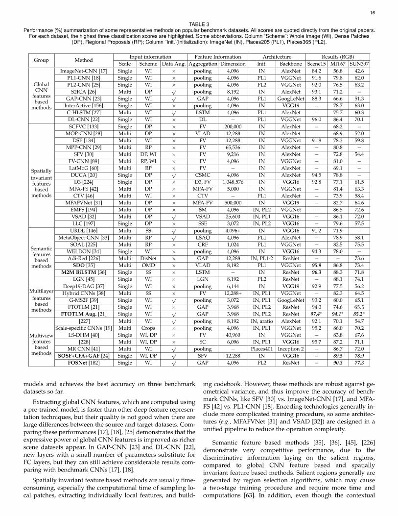
16

TABLE 3Performance (%) summarization of some representative methods on popular benchmark datasets. All scores are quoted directly from the original papers.

For each dataset, the highest three classification scores are highlighted. Some abbreviations. Column “Scheme”: Whole Image (WI), Dense Patches(DP), Regional Proposals (RP); Column “Init.”(Initialization): ImageNet (IN), Places205 (PL1), Places365 (PL2).

Group MethodInput information Feature Information Architecture Results (RGB)

Scale Scheme Data Aug. Aggregation Dimension Init. Backbone Scene15 MIT67 SUN397

GlobalCNN

featuresbased

methods

ImageNet-CNN [17] Single WI × pooling 4,096 IN AlexNet 84.2 56.8 42.6PL1-CNN [18] Single WI × pooling 4,096 PL1 VGGNet 91.6 79.8 62.0PL2-CNN [25] Single WI × pooling 4,096 PL2 VGGNet 92.0 76.5 63.2

S2ICA [26] Multi DP√

pooling 8,192 IN AlexNet 93.1 71.2 −GAP-CNN [23] Single WI

√GAP 4,096 PL1 GoogLeNet 88.3 66.6 51.3

InterActive [156] Single WI × pooling 4,096 IN VGG19 − 78.7 63.0C-HLSTM [27] Multi WI

√LSTM 4,096 PL1 AlexNet − 75.7 60.3

DL-CNN [22] Single WI × DL − PL1 VGGNet 96.0 86.4 70.1

Spatiallyinvariantfeaturesbased

methods

SCFVC [133] Single DP × FV 200,000 IN AlexNet − 68.2 −MOP-CNN [28] Multi DP × VLAD 12,288 IN AlexNet − 68.9 52.0

DSP [134] Multi WI × FV 12,288 IN VGGNet 91.8 78.3 59.8MPP-CNN [29] Multi RP × FV 65,536 IN AlexNet − 80.8 −

SFV [30] Multi DP, WI × FV 9,216 IN AlexNet − 72.8 54.4FV-CNN [89] Multi RP, WI × FV 4,096 IN VGGNet − 81.0 −LatMoG [60] Multi RP × FV − IN AlexNet − 69.1 −DUCA [20] Single DP

√CSMC 4,096 IN AlexNet 94.5 78.8 −

D3 [224] Single DP × D3, FV 1,048,576 IN VGG16 92.8 77.1 61.5MFA-FS [42] Multi DP × MFA-FV 5,000 IN VGGNet − 81.4 63.3

CTV [46] Multi WI × CTV − PL1 AlexNet − 73.9 58.4MFAFVNet [31] Multi DP × MFA-FV 500,000 IN VGG19 − 82.7 64.6

EMFS [194] Multi DP × SM 4,096 IN, PL2 VGGNet − 86.5 72.6VSAD [32] Multi DP

√VSAD 25,600 IN, PL1 VGG16 − 86.1 72.0

LLC [197] Single DP × SSE 3,072 IN, PL2 VGG16 − 79.6 57.5

Semanticfeaturesbased

methods

URDL [146] Multi SS√

pooling 4,096+ IN VGG16 91.2 71.9 −MetaObject-CNN [33] Multi RP

√LSAQ 4,096 PL1 AlexNet − 78.9 58.1

SOAL [225] Multi RP × CRF 1,024 PL1 VGGNet − 82.5 75.5WELDON [34] Single WI × pooling 4,096 IN VGG16 94.3 78.0 −Adi-Red [226] Multi DisNet × GAP 12,288 IN, PL1-2 ResNet − − 73.6

SDO [35] Multi OMD × VLAD 8,192 PL1 VGGNet 95.9 86.8 73.4M2M BiLSTM [36] Single SS × LSTM − IN ResNet 96.3 88.3 71.8

LGN [45] Single WI × LGN 8,192 PL2 ResNet − 88.1 74.1

Multilayerfeaturesbased

methods

Deep19-DAG [37] Single WI × pooling 6,144 IN VGG19 92.9 77.5 56.2Hybrid CNNs [38] Multi SS × FV 12,288+ IN, PL1 VGGNet − 82.3 64.5

G-MS2F [39] Single WI√

pooling 3,072 IN, PL1 GoogLeNet 93.2 80.0 65.1FTOTLM [21] Single WI × GAP 3,968 IN, PL2 ResNet 94.0 74.6 65.5

FTOTLM Aug. [21] Single WI√

GAP 3,968 IN, PL2 ResNet 97.4∗ 94.1∗ 85.2∗

Multiviewfeaturesbased

methods

[227] Multi WI√

pooling 8,192 IN, aratio AlexNet 92.1 70.1 54.7Scale-specific CNNs [19] Multi Crops × pooling 4,096 IN, PL1 VGGNet 95.2 86.0 70.2

LS-DHM [40] Single WI, DP × FV 40,960 IN VGGNet − 83.8 67.6[228] Multi WI, DP × SC 6,096 IN, PL1 VGG16 95.7 87.2 71.1

MR CNN [41] Multi WI√

pooling − Places401 Inception 2 − 86.7 72.0SOSF+CFA+GAF [24] Single WI, DP

√SFV 12,288 IN VGG16 − 89.5 78.9

FOSNet [182] Single WI√

GAP 4,096 PL2 ResNet − 90.3 77.3

models and achieves the best accuracy on three benchmarkdatasets so far.

Extracting global CNN features, which are computed usinga pre-trained model, is faster than other deep feature represen-tation techniques, but their quality is not good when there arelarge differences between the source and target datasets. Com-paring these performances [17], [18], [25] demonstrates that theexpressive power of global CNN features is improved as richerscene datasets appear. In GAP-CNN [23] and DL-CNN [22],new layers with a small number of parameters substitute forFC layers, but they can still achieve considerable results com-paring with benchmark CNNs [17], [18].

Spatially invariant feature based methods are usually time-consuming, especially the computational time of sampling lo-cal patches, extracting individually local features, and build-

ing codebook. However, these methods are robust against ge-ometrical variance, and thus improve the accuracy of bench-mark CNNs, like SFV [30] vs. ImageNet-CNN [17], and MFA-FS [42] vs. PL1-CNN [18]. Encoding technologies generally in-clude more complicated training procedure, so some architec-tures (e.g., MFAFVNet [31] and VSAD [32]) are designed in aunified pipeline to reduce the operation complexity.

Semantic feature based methods [35], [36], [45], [226]demonstrate very competitive performance, due to thediscriminative information laying on the salient regions,compared to global CNN feature based and spatiallyinvariant feature based methods. Salient regions generally aregenerated by region selection algorithms, which may causea two-stage training procedure and require more time andcomputations [63]. In addition, even though the contextual

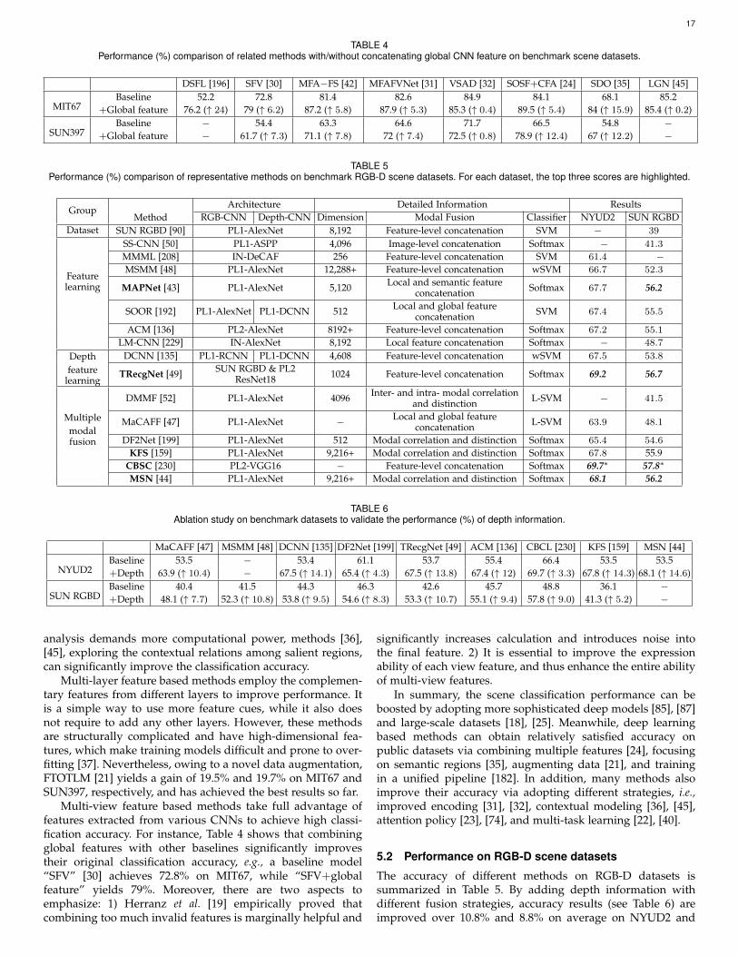
17

TABLE 4Performance (%) comparison of related methods with/without concatenating global CNN feature on benchmark scene datasets.

DSFL [196] SFV [30] MFA−FS [42] MFAFVNet [31] VSAD [32] SOSF+CFA [24] SDO [35] LGN [45]

MIT67Baseline 52.2 72.8 81.4 82.6 84.9 84.1 68.1 85.2

+Global feature 76.2 (↑ 24) 79 (↑ 6.2) 87.2 (↑ 5.8) 87.9 (↑ 5.3) 85.3 (↑ 0.4) 89.5 (↑ 5.4) 84 (↑ 15.9) 85.4 (↑ 0.2)

SUN397Baseline − 54.4 63.3 64.6 71.7 66.5 54.8 −

+Global feature − 61.7 (↑ 7.3) 71.1 (↑ 7.8) 72 (↑ 7.4) 72.5 (↑ 0.8) 78.9 (↑ 12.4) 67 (↑ 12.2) −

TABLE 5Performance (%) comparison of representative methods on benchmark RGB-D scene datasets. For each dataset, the top three scores are highlighted.

GroupMethod

Architecture Detailed Information ResultsRGB-CNN Depth-CNN Dimension Modal Fusion Classifier NYUD2 SUN RGBD

Dataset SUN RGBD [90] PL1-AlexNet 8,192 Feature-level concatenation SVM − 39

Featurelearning

SS-CNN [50] PL1-ASPP 4,096 Image-level concatenation Softmax − 41.3

MMML [208] IN-DeCAF 256 Feature-level concatenation SVM 61.4 −MSMM [48] PL1-AlexNet 12,288+ Feature-level concatenation wSVM 66.7 52.3

MAPNet [43] PL1-AlexNet 5,120 Local and semantic featureconcatenation Softmax 67.7 56.2

SOOR [192] PL1-AlexNet PL1-DCNN 512 Local and global featureconcatenation SVM 67.4 55.5

ACM [136] PL2-AlexNet 8192+ Feature-level concatenation Softmax 67.2 55.1

LM-CNN [229] IN-AlexNet 8,192 Local feature concatenation Softmax − 48.7

Depthfeature

learning

DCNN [135] PL1-RCNN PL1-DCNN 4,608 Feature-level concatenation wSVM 67.5 53.8

TRecgNet [49] SUN RGBD & PL2ResNet18 1024 Feature-level concatenation Softmax 69.2 56.7

Multiplemodalfusion

DMMF [52] PL1-AlexNet 4096 Inter- and intra- modal correlationand distinction L-SVM − 41.5

MaCAFF [47] PL1-AlexNet − Local and global featureconcatenation L-SVM 63.9 48.1

DF2Net [199] PL1-AlexNet 512 Modal correlation and distinction Softmax 65.4 54.6

KFS [159] PL1-AlexNet 9,216+ Modal correlation and distinction Softmax 67.8 55.9CBSC [230] PL2-VGG16 − Feature-level concatenation Softmax 69.7∗ 57.8∗

MSN [44] PL1-AlexNet 9,216+ Modal correlation and distinction Softmax 68.1 56.2

TABLE 6Ablation study on benchmark datasets to validate the performance (%) of depth information.

MaCAFF [47] MSMM [48] DCNN [135] DF2Net [199] TRecgNet [49] ACM [136] CBCL [230] KFS [159] MSN [44]

NYUD2Baseline 53.5 − 53.4 61.1 53.7 55.4 66.4 53.5 53.5+Depth 63.9 (↑ 10.4) − 67.5 (↑ 14.1) 65.4 (↑ 4.3) 67.5 (↑ 13.8) 67.4 (↑ 12) 69.7 (↑ 3.3) 67.8 (↑ 14.3) 68.1 (↑ 14.6)

SUN RGBDBaseline 40.4 41.5 44.3 46.3 42.6 45.7 48.8 36.1 −+Depth 48.1 (↑ 7.7) 52.3 (↑ 10.8) 53.8 (↑ 9.5) 54.6 (↑ 8.3) 53.3 (↑ 10.7) 55.1 (↑ 9.4) 57.8 (↑ 9.0) 41.3 (↑ 5.2) −

analysis demands more computational power, methods [36],[45], exploring the contextual relations among salient regions,can significantly improve the classification accuracy.

Multi-layer feature based methods employ the complemen-tary features from different layers to improve performance. Itis a simple way to use more feature cues, while it also doesnot require to add any other layers. However, these methodsare structurally complicated and have high-dimensional fea-tures, which make training models difficult and prone to over-fitting [37]. Nevertheless, owing to a novel data augmentation,FTOTLM [21] yields a gain of 19.5% and 19.7% on MIT67 andSUN397, respectively, and has achieved the best results so far.

Multi-view feature based methods take full advantage offeatures extracted from various CNNs to achieve high classi-fication accuracy. For instance, Table 4 shows that combiningglobal features with other baselines significantly improvestheir original classification accuracy, e.g., a baseline model“SFV” [30] achieves 72.8% on MIT67, while “SFV+globalfeature” yields 79%. Moreover, there are two aspects toemphasize: 1) Herranz et al. [19] empirically proved thatcombining too much invalid features is marginally helpful and

significantly increases calculation and introduces noise intothe final feature. 2) It is essential to improve the expressionability of each view feature, and thus enhance the entire abilityof multi-view features.

In summary, the scene classification performance can beboosted by adopting more sophisticated deep models [85], [87]and large-scale datasets [18], [25]. Meanwhile, deep learningbased methods can obtain relatively satisfied accuracy onpublic datasets via combining multiple features [24], focusingon semantic regions [35], augmenting data [21], and trainingin a unified pipeline [182]. In addition, many methods alsoimprove their accuracy via adopting different strategies, i.e.,improved encoding [31], [32], contextual modeling [36], [45],attention policy [23], [74], and multi-task learning [22], [40].

5.2 Performance on RGB-D scene datasets

The accuracy of different methods on RGB-D datasets issummarized in Table 5. By adding depth information withdifferent fusion strategies, accuracy results (see Table 6) areimproved over 10.8% and 8.8% on average on NYUD2 and

18

SUN RGBD datasets, respectively. Since depth data provideextra information to train classification model, this observationis within expectation. Noteworthily, it is more difficult toimprove the effect on a large dataset (SUN RGBD) than a smalldataset (NYUD2). Moreover, the best results on NYUD2 andSUN RGBD datasets achieved by CBSC [230] are as high as69.7% and 57.84%, respectively.

RGB-D scene data for training are relatively limited, whilethe dimension of scene features is high. Hence, SupportVector Machines (SVMs) are commonly used in RGB-D sceneclassification [48], [90], [135], [208] in the early stages. Thanksto data augmentation and back-propagation, Softmax classifierbecomes progressively popular, and it is an important reasonto yield a comparable performance [43], [44], [49], [230].

Many methods, such as [47], [52], fine-tune RGB-CNNs toextract deep features of depth modality, where the trainingprocess is simple, and the computational cost is low. To adaptto depth data, Song et al. [135], [231] used weakly-supervisedlearning to train depth-specific models from scratch, whichachieves a gain of 3.5% accuracy, compared to the fine-tunedRGB-CNN. TRecgNet [49], which is based on semi-supervisedlearning, requires complicated training process and highcomputational cost, but it obtains comparable results (69.2%on NYUD2 and 56.7% on SUN RGBD).

Feature-level fusion based methods are commonly useddue to their high cost-effectiveness, e.g., [43], [136], [230].Along this way, consistent-feature based, and distinctive-feature based modal fusion use complex fusion layer withhigh cost, like inference speed and training complexity, butthey generally yield more effective features [44], [159], [199].

We can observe that the field of RGB-D scene classificationhas constantly been improving. Weakly-supervised andsemi-supervised learning are useful to learn depth-specificfeatures [48], [49], [135]. Moreover, multi-modal feature fusionis a major issue to improve performance on public datasets [44],[199], [230]. In addition, effective strategies (like contextualstrategy [136], [192] and attention mechanism [43], [44]) arealso popular for RGB-D scene classification. Nevertheless, theaccuracy achieved by current methods is far from expectationand there remains significant rooms for future improvement.

6 CONCLUSION AND OUTLOOK

As a contemporary survey for scene classification using deeplearning, this paper has highlighted the recent achievements,provided some structural taxonomy for various methods ac-cording to their roles in scene representation for scene clas-sification, analyzed their advantages and limitations, summa-rized existing popular scene datasets, and discussed perfor-mance for the most representative approaches. Despite greatprogress, there are still many unsolved problems. Thus in thissection, we will point out these problems and introduce somepromising trends for future research. We hope that this surveynot only provides a better understanding of scene classificationfor researchers but also stimulates future research activities.

Develop more advanced network frameworks. Withthe development of deep CNN architectures, from genericCNNs [17], [85], [86], [87] to scene-specific CNNs [22], [23],the accuracy of scene classification is getting increasinglycomparable. Nevertheless, there still exists lots of works to beexplored on the theoretical research of deep learning [232].It is a further direction to solidify the theoretical basis so asto get more advanced network frameworks. In particular,it is essential to design specific frameworks for scene

classification, such as using automated Neural ArchitectureSearch (NAS) [233], [234], or according to scene attributes.

Release rich scene datasets. Deep learning based modelsrequire enormous amounts of data to initialize their parametersso that they can learn the scene knowledge well [18], [25].However, compared to scenes of real world, the publiclyavailable datasets are not large or rich enough, so it is essentialto release datasets that encompass richness and high-diversityof environmental scenes [235], especially large-scale RGB-Dscene datasets. As opposed to object/texture datasets, sceneappearance may be changed dramatically as time goes by,and there emerges new functional scenes as humans developactivity places. Therefore, it requires updating the originalscene data and releasing new scene datasets regularly.

Reduce the dependence of labeled scene images. The suc-cess of deep learning heavily relies on gargantuan amountsof labeled images. However, the labeled training images arealways very limited, so supervised learning is not scalable inthe absence of fully labeled training data and its generalizationability to classify scenes frequently deteriorates. Therefore, itis desirable to reduce dependence on large amounts of labeleddata. To alleviate this difficulty, if with large numbers of unla-bel data, it is necessary to further study semi-supervised learn-ing [236], unsupervised learning [237], or self-supervised learn-ing [238]. Even more constrained, without any unlabel trainingdata, the ability to learn from only few labeled images, small-sample learning [239], is also appealing.

Few shot scene classification. The success of generic CNNsfor scene classification relies heavily on gargantuan amountsof labeled training data [72]. Due to the large intra-variationamong scenes, scene datasets cannot cover various classes sothat the performance of CNNs frequently deteriorates and failsto generalize well. In contrast, humans can learn a visual con-cept quickly from very few given examples and often gener-alize well [240], [241]. Inspired by this, domain adaptation ap-proaches utilize the knowledge of labeled data in task-relevantdomains to execute new tasks in target domain [242], [243].Furthermore, domain generalization methods aim at learninggeneric representation from multiple task-irrelevant domainsto generalize unseen scenarios [244], [245].

Robust scene classification. Once scene classification in thelaboratory environment is deployed in the real application sce-nario, there will still be a variety of unacceptable phenomena,that is, the robustness in open environments is a bottleneck torestrict pattern recognition technology. The main reasons whythe pattern recognition systems are not robust are basic as-sumptions, e.g., closed world assumption, independent identi-cal distribution and big data assumption [246], which are maindifferences between machine learning and human intelligence;hence, it is a fundamental challenge to improve the robustnessby breaking these assumptions. It is a nature consider via uti-lizing adversarial training and optimization [247], [248], [249],which have been applied to pattern recognition [250], [251].

Realtime scene classification. Many methods for sceneclassification, trained in a multiple-stage manner, are com-putationally expensive for current mobile/wearable devices,which have limited storage and computational capability,therefore researchers have begun to develop convenient andefficient unified networks (encapsulating all computation ina one-stage network) [22], [31], [44]. Moreover, it is also achallenge to keep the model scalable and efficient well whenbig data from smart wearables and mobile applications isgrowing rapidly in size temporally or spatially [252].

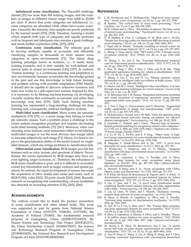
19

Imbalanced scene classification. The Places365 challengedataset [25] has more than 8M training images, and the num-bers of images in different classes range from 4,000 to 30,000per class. It shows that scene categories are imbalanced, i.e.,some categories are abundant while others have scarce exam-ples. Generally, the minority class samples are poorly predictedby the learned model [253], [254]. Therefore, learning a modelwhich respects both type of categories and equally performswell on frequent and infrequent ones remains a great challengeand needs further exploration [254], [255], [256].

Continuous scene classification. The ultimate goal isto develop methods capable of accurately and efficientlyclassifying samples in thousands or more unseen scenecategories in open environments [72]. The classic deeplearning paradigm learns in isolation, i.e., it needs manytraining examples and is only suitable for well-defined andnarrow tasks in closed environments [142], [257]. In contrast,“human learning” is a continuous learning and adaptation tonew environments: humans accumulate the knowledge gainedin the past and use this knowledge to help future learningand problem solving with possible adaptations [258]. Ideally,it should also be capable to discover unknown scenarios andlearn new works in a self-supervised manner. Inspired by this,it is necessary to do lifelong machine learning via developingversatile systems that continually accumulate and refine theirknowledge over time [259], [260]. Such lifelong machinelearning has represented a long-standing challenge for deeplearning and, consequently, artificial intelligence systems.

Multi-label scene classification. Many scenes are semanticmultiplicity [73], [75], i.e., a scene image may belong to multi-ple semantic classes. Such a problem poses a challenge to theclassic pattern recognition paradigm and requires developingmulti-label learning methods [75], [261]. Moreover, when con-structing scene datasets, most researchers either avoid labelingmulti-label images or use the most obvious class (single label)to annotate subjectively each image [73]. Hence, it is hard to im-prove the generalization ability of the model trained on single-label datasets, which also brings problems to classification task.

Other-modal scene classification. RGB images provide keyfeatures such as color, texture, and spectrum of objects. Never-theless, the scenes reproduced by RGB images may have un-even lighting, target occlusion, etc. Therefore, the robustness ofRGB scene classification is poor, and it is difficult to accuratelyextract key information such as target contours and spatial po-sitions. In contrast, the rapid development of sensors has madethe acquisition of other modal data easier and easier, such asRGB-D [90], video [262], 3D point clouds [263], [264]. Recently,research on recognizing and understanding various modalitieshas attracted an increasing attention [135], [265], [266].

ACKNOWLEDGMENTS

The authors would like to thank the pioneer researchersin scene classification and other related fields. This workwas supported in part by grants from National ScienceFoundation of China (61872379, 91846301, 61571005), theAcademy of Finland (331883), the fundamental researchprogram of Guangdong, China (2020B1515310023), theHunan Science and Technology Plan Project (2019GK2131),the China Scholarship Council (201806155037), the Scienceand Technology Research Program of Guangzhou, China(201804010429), the National Key Research and DevelopmentProgram of China (2016YFB1200402020).

REFERENCES

[1] J. M. Henderson and A. Hollingworth, “High-level scene percep-tion,” Annual review of psychology, vol. 50, no. 1, pp. 243–271, 1999.

[2] R. Epstein, “The cortical basis of visual scene processing,” VisualCognition, vol. 12, no. 6, pp. 954–978, 2005.

[3] M. R. Greene and A. Oliva, “The briefest of glances: The time courseof natural scene understanding,” Psychological Science, vol. 20, no. 4,pp. 464–472, 2009.

[4] D. B. Walther, B. Chai, E. Caddigan, D. M. Beck, and L. Fei-Fei,“Simple line drawings suffice for functional MRI decoding of naturalscene categories,” PNAS, vol. 108, no. 23, pp. 9661–9666, 2011.

[5] J. Vogel and B. Schiele, “Semantic modeling of natural scenes forcontent-based image retrieval,” IJCV, vol. 72, no. 2, pp. 133–157, 2007.

[6] L. Zheng, Y. Yang, and Q. Tian, “SIFT meets CNN: A decade surveyof instance retrieval,” IEEE TPAMI, vol. 40, no. 5, pp. 1224–1244,2017.

[7] W. Zhang, X. Yu, and X. He, “Learning bidirectional temporalcues for video-based person re-identification,” IEEE TCSVT, vol. 28,no. 10, pp. 2768–2776, 2017.

[8] J. Hou, H. Zeng, J. Zhu, J. Hou, J. Chen, and K.-K. Ma, “Deepquadruplet appearance learning for vehicle re-identification,” IEEETVT, vol. 68, no. 9, pp. 8512–8522, 2019.

[9] T. Zhang, S. Liu, C. Xu, and H. Lu, “Mining semantic contextinformation for intelligent video surveillance of traffic scenes,” IEEETII, vol. 9, no. 1, pp. 149–160, 2012.

[10] G. Sreenu and M. S. Durai, “Intelligent video surveillance: A reviewthrough deep learning techniques for crowd analysis,” Journal of BigData, vol. 6, no. 1, p. 48, 2019.

[11] A. H. Behzadan and V. R. Kamat, “Integrated information modelingand visual simulation of engineering operations using dynamicaugmented reality scene graphs,” ITcon, vol. 16, no. 17, pp. 259–278,2011.

[12] A. Y. Nee, S. Ong, G. Chryssolouris, and D. Mourtzis, “Augmentedreality applications in design and manufacturing,” CIRP annals,vol. 61, no. 2, pp. 657–679, 2012.

[13] K. Muhammad, J. Ahmad, and S. W. Baik, “Early fire detection usingconvolutional neural networks during surveillance for effectivedisaster management,” Neurocomputing, vol. 288, pp. 30–42, 2018.

[14] S. Lazebnik, C. Schmid, and J. Ponce, “Beyond bags of features:Spatial pyramid matching for recognizing natural scene categories,”in CVPR, vol. 2, 2006, pp. 2169–2178, https://figshare.com/articles/15-Scene Image Dataset/7007177.

[15] L.-J. Li, H. Su, L. Fei-Fei, and E. P. Xing, “Object bank: A high-level image representation for scene classification & semantic featuresparsification,” in NeurIPS, 2010, pp. 1378–1386.

[16] R. Margolin, L. Zelnik-Manor, and A. Tal, “OTC: A novel localdescriptor for scene classification,” in ECCV, 2014, pp. 377–391.

[17] A. Krizhevsky, I. Sutskever, and G. E. Hinton, “Imagenetclassification with deep convolutional neural networks,” in NeurIPS,2012, pp. 1097–1105.

[18] B. Zhou, A. Lapedriza, J. Xiao, A. Torralba, and A. Oliva,“Learning deep features for scene recognition using placesdatabase,” in NeurIPS, 2014, pp. 487–495, http://places.csail.mit.edu/downloadData.html.

[19] L. Herranz, S. Jiang, and X. Li, “Scene recognition with CNNs:Objects, scales and dataset bias,” in CVPR, 2016, pp. 571–579.

[20] S. H. Khan, M. Hayat, M. Bennamoun, R. Togneri, and F. A. Sohel, “Adiscriminative representation of convolutional features for indoorscene recognition,” IEEE TIP, vol. 25, no. 7, pp. 3372–3383, 2016.

[21] S. Liu, G. Tian, and Y. Xu, “A novel scene classification modelcombining ResNet based transfer learning and data augmentationwith a filter,” Neurocomputing, vol. 338, pp. 191–206, 2019.

[22] Y. Liu, Q. Chen, W. Chen, and I. Wassell, “Dictionary learninginspired deep network for scene recognition,” in AAAI, 2018.

[23] B. Zhou, A. Khosla, A. Lapedriza, A. Oliva, and A. Torralba,“Learning deep features for discriminative localization,” in CVPR,2016, pp. 2921–2929.

[24] N. Sun, W. Li, J. Liu, G. Han, and C. Wu, “Fusing object semanticsand deep appearance features for scene recognition,” IEEE TCSVT,vol. 29, no. 6, pp. 1715–1728, 2018.

[25] B. Zhou, A. Lapedriza, A. Khosla, A. Oliva, and A. Torralba, “Places:A 10 million image database for scene recognition,” IEEE TPAMI,vol. 40, no. 6, pp. 1452–1464, 2017, http://places2.csail.mit.edu/download.html.

[26] M. Hayat, S. H. Khan, M. Bennamoun, and S. An, “A spatiallayout and scale invariant feature representation for indoor sceneclassification,” IEEE TIP, vol. 25, no. 10, pp. 4829–4841, 2016.

[27] Z. Zuo, B. Shuai, G. Wang, X. Liu, X. Wang, B. Wang, and Y. Chen,“Learning contextual dependence with convolutional hierarchical

20

recurrent neural networks,” IEEE TIP, vol. 25, no. 7, pp. 2983–2996,2016.

[28] Y. Gong, L. Wang, R. Guo, and S. Lazebnik, “Multi-scale orderlesspooling of deep convolutional activation features,” in ECCV, 2014,pp. 392–407.

[29] D. Yoo, S. Park, J.-Y. Lee, and I. So Kweon, “Multi-scale pyramidpooling for deep convolutional representation,” in CVPRW, 2015,pp. 71–80.

[30] M. Dixit, S. Chen, D. Gao, N. Rasiwasia, and N. Vasconcelos, “Sceneclassification with semantic fisher vectors,” in CVPR, 2015, pp. 2974–2983.

[31] Y. Li, M. Dixit, and N. Vasconcelos, “Deep scene image classificationwith the MFAFVNet,” in ICCV, 2017, pp. 5746–5754.

[32] Z. Wang, L. Wang, Y. Wang, B. Zhang, and Y. Qiao, “Weaklysupervised patchnets: Describing and aggregating local patches forscene recognition,” IEEE TIP, vol. 26, no. 4, pp. 2028–2041, 2017.

[33] R. Wu, B. Wang, W. Wang, and Y. Yu, “Harvesting discriminativemeta objects with deep CNN features for scene classification,” inICCV, 2015, pp. 1287–1295.

[34] T. Durand, N. Thome, and M. Cord, “WELDON: Weakly supervisedlearning of deep convolutional neural networks,” in CVPR, 2016, pp.4743–4752.

[35] X. Cheng, J. Lu, J. Feng, B. Yuan, and J. Zhou, “Scene recognitionwith objectness,” Pattern Recognition, vol. 74, pp. 474–487, 2018.

[36] C. Laranjeira, A. Lacerda, and E. R. Nascimento, “On modelingcontext from objects with a long short-term memory for indoor scenerecognition,” in SIBGRAPI, 2019, pp. 249–256.

[37] S. Yang and D. Ramanan, “Multi-scale recognition with DAG-CNNs,” in ICCV, 2015, pp. 1215–1223.

[38] G.-S. Xie, X.-Y. Zhang, S. Yan, and C.-L. Liu, “Hybrid CNNand dictionary-based models for scene recognition and domainadaptation,” IEEE TCSVT, vol. 27, no. 6, pp. 1263–1274, 2015.

[39] P. Tang, H. Wang, and S. Kwong, “G-MS2F: Googlenet basedmulti-stage feature fusion of deep CNN for scene recognition,”Neurocomputing, vol. 225, pp. 188–197, 2017.

[40] S. Guo, W. Huang, L. Wang, and Y. Qiao, “Locally supervised deephybrid model for scene recognition,” IEEE TIP, vol. 26, no. 2, pp.808–820, 2016.

[41] L. Wang, S. Guo, W. Huang, Y. Xiong, and Y. Qiao, “Knowledgeguided disambiguation for large-scale scene classification withmulti-resolution CNNs,” IEEE TIP, vol. 26, no. 4, pp. 2055–2068,2017.

[42] M. D. Dixit and N. Vasconcelos, “Object based scene representationsusing fisher scores of local subspace projections,” in NeurIPS, 2016,pp. 2811–2819.

[43] Y. Li, Z. Zhang, Y. Cheng, L. Wang, and T. Tan, “MAPNet:Multi-modal attentive pooling network for RGB-D indoor sceneclassification,” Pattern Recognition, vol. 90, pp. 436–449, 2019.

[44] Z. Xiong, Y. Yuan, and Q. Wang, “MSN: Modality separationnetworks for RGB-D scene recognition,” Neurocomputing, vol. 373,pp. 81–89, 2020.

[45] G. Chen, X. Song, H. Zeng, and S. Jiang, “Scene recognition withprototype-agnostic scene layout,” IEEE TIP, vol. 29, pp. 5877–5888,2020.

[46] P. Wei, F. Qin, F. Wan, Y. Zhu, J. Jiao, and Q. Ye, “Correlated topicvector for scene classification,” IEEE TIP, vol. 26, no. 7, pp. 3221–3234, 2017.

[47] A. Wang, J. Cai, J. Lu, and T.-J. Cham, “Modality and componentaware feature fusion for RGB-D scene classification,” in CVPR, 2016,pp. 5995–6004.

[48] X. Song, S. Jiang, and L. Herranz, “Combining models from multiplesources for RGB-D scene recognition.” in IJCAI, 2017, pp. 4523–4529.

[49] D. Du, L. Wang, H. Wang, K. Zhao, and G. Wu, “Translate-to-recognize networks for RGB-D scene recognition,” in CVPR, 2019,pp. 11 836–11 845.

[50] Y. Liao, S. Kodagoda, Y. Wang, L. Shi, and Y. Liu, “Understand scenecategories by objects: A semantic regularized scene classifier usingconvolutional neural networks,” in CRA, 2016, pp. 2318–2325.

[51] Y. Cheng, R. Cai, Z. Li, X. Zhao, and K. Huang, “Locality-sensitive deconvolution networks with gated fusion for RGB-Dindoor semantic segmentation,” in CVPR, 2017, pp. 3029–3037.

[52] H. Zhu, J.-B. Weibel, and S. Lu, “Discriminative multi-modal featurefusion for RGB-D indoor scene recognition,” in CVPR, 2016, pp.2969–2976.

[53] R. Girshick, “Fast R-CNN,” in ICCV, 2015, pp. 1440–1448.[54] S. Ren, K. He, R. Girshick, and J. Sun, “Faster R-CNN: Towards real-

time object detection with region proposal networks,” IEEE TPAMI,vol. 39, no. 6, pp. 1137–1149, 2016.

[55] V. Badrinarayanan, A. Kendall, and R. Cipolla, “SegNet: A deep con-volutional encoder-decoder architecture for image segmentation,”IEEE TPAMI, vol. 39, no. 12, pp. 2481–2495, 2017.

[56] L.-C. Chen, G. Papandreou, I. Kokkinos, K. Murphy, and A. L. Yuille,“Deeplab: Semantic image segmentation with deep convolutionalnets, atrous convolution, and fully connected crfs,” IEEE TPAMI,vol. 40, no. 4, pp. 834–848, 2017.

[57] S. Cai, J. Huang, D. Zeng, X. Ding, and J. Paisley, “MEnet: A metricexpression network for salient object segmentation,” in IJCAI, 2018,pp. 598–605.

[58] J. Deng, W. Dong, R. Socher, L.-J. Li, K. Li, and L. Fei-Fei, “Imagenet:A large-scale hierarchical image database,” in CVPR, 2009, pp. 248–255, http://image-net.org/download.

[59] J. Xiao, J. Hays, K. A. Ehinger, A. Oliva, and A. Torralba, “Sundatabase: Large-scale scene recognition from abbey to zoo,” in CVPR,2010, pp. 3485–3492, http://places2.csail.mit.edu/download.html.

[60] R. G. Cinbis, J. Verbeek, and C. Schmid, “Approximate fisher kernelsof non-iid image models for image categorization,” IEEE TPAMI,vol. 38, no. 6, pp. 1084–1098, 2015.

[61] X. Wei, S. L. Phung, and A. Bouzerdoum, “Visual descriptors forscene categorization: Experimental evaluation,” AI Review, vol. 45,no. 3, pp. 333–368, 2016.

[62] G. Cheng, J. Han, and X. Lu, “Remote sensing image sceneclassification: Benchmark and state of the art,” Proceedings of the IEEE,vol. 105, no. 10, pp. 1865–1883, 2017.

[63] L. Xie, F. Lee, L. Liu, K. Kotani, and Q. Chen, “Scene recognition: Acomprehensive survey,” Pattern Recognition, vol. 102, p. 107205, 2020.

[64] K. Nogueira, O. A. Penatti, and J. A. Dos Santos, “Towards betterexploiting convolutional neural networks for remote sensing sceneclassification,” Pattern Recognition, vol. 61, pp. 539–556, 2017.

[65] F. Hu, G.-S. Xia, J. Hu, and L. Zhang, “Transferring deepconvolutional neural networks for the scene classification of high-resolution remote sensing imagery,” Remote Sensing, vol. 7, no. 11,pp. 14 680–14 707, 2015.

[66] A. Mesaros, T. Heittola, and T. Virtanen, “Tut database for acousticscene classification and sound event detection,” in EUSIPCO, 2016,pp. 1128–1132.

[67] Z. Ren, K. Qian, Y. Wang, Z. Zhang, V. Pandit, A. Baird, andB. Schuller, “Deep scalogram representations for acoustic sceneclassification,” JAS, vol. 5, no. 3, pp. 662–669, 2018.

[68] S. Lowry, N. Sunderhauf, P. Newman, J. J. Leonard, D. Cox, P. Corke,and M. J. Milford, “Visual place recognition: A survey,” IEEE T-RO,vol. 32, no. 1, pp. 1–19, 2015.

[69] R. Arandjelovic, P. Gronat, A. Torii, T. Pajdla, and J. Sivic,“NetVLAD: CNN architecture for weakly supervised placerecognition,” in CVPR, 2016, pp. 5297–5307.

[70] L. W. Renninger and J. Malik, “When is scene identification justtexture recognition?” Vision research, vol. 44, no. 19, pp. 2301–2311,2004.

[71] L. Liu, J. Chen, P. Fieguth, G. Zhao, R. Chellappa, and M. Pietikainen,“From BoW to CNN: Two decades of texture representation fortexture classification,” IJCV, vol. 127, no. 1, pp. 74–109, 2019.

[72] L. Liu, W. Ouyang, X. Wang, P. Fieguth, J. Chen, X. Liu, andM. Pietikainen, “Deep learning for generic object detection: Asurvey,” IJCV, vol. 128, no. 2, pp. 261–318, 2020.

[73] M. R. Boutell, J. Luo, X. Shen, and C. M. Brown, “Learning multi-label scene classification,” Pattern Recognition, vol. 37, no. 9, pp. 1757–1771, 2004.

[74] A. Lopez-Cifuentes, M. Escudero-Vinolo, J. Bescos, and A. Garcıa-Martın, “Semantic-aware scene recognition,” Pattern Recognition, vol.102, p. 107256, 2020.

[75] M.-L. Zhang and Z.-H. Zhou, “Multi-label learning by instancedifferentiation,” in AAAI, vol. 7, 2007, pp. 669–674.

[76] D. G. Lowe, “Object recognition from local scale-invariant features,”in IJCV, vol. 2, 1999, pp. 1150–1157.

[77] A. Oliva and A. Torralba, “Modeling the shape of the scene: Aholistic representation of the spatial envelope,” IJCV, vol. 42, no. 3,pp. 145–175, 2001.

[78] N. Dalal and B. Triggs, “Histograms of oriented gradients for humandetection,” in CVPR, vol. 1, 2005, pp. 886–893.

[79] J. Wu and J. M. Rehg, “CENTRIST: A visual descriptor for scenecategorization,” IEEE TPAMI, vol. 33, no. 8, pp. 1489–1501, 2010.

[80] J. Sivic and A. Zisserman, “Video google: A text retrieval approachto object matching in videos,” in ICCV, vol. 2, 2003, p. 14701477.

[81] J. Sanchez, F. Perronnin, T. Mensink, and J. Verbeek, “Imageclassification with the Fisher vector: Theory and practice,” IJCV, vol.105, no. 3, pp. 222–245, 2013.

[82] H. Jegou, M. Douze, C. Schmid, and P. Perez, “Aggregating localdescriptors into a compact image representation,” in CVPR, 2010,pp. 3304–3311.

[83] L.-J. Li, H. Su, Y. Lim, and L. Fei-Fei, “Objects as attributes for sceneclassification,” in ECCV, 2010, pp. 57–69.

21

[84] M. Juneja, A. Vedaldi, C. Jawahar, and A. Zisserman, “Blocks thatshout: Distinctive parts for scene classification,” in CVPR, 2013, pp.923–930.

[85] K. Simonyan and A. Zisserman, “Very deep convolutional networksfor large-scale image recognition,” ICLR, 2015.

[86] C. Szegedy, W. Liu, Y. Jia, P. Sermanet, S. Reed, D. Anguelov,D. Erhan, V. Vanhoucke, and A. Rabinovich, “Going deeper withconvolutions,” in CVPR, 2015, pp. 1–9.

[87] K. He, X. Zhang, S. Ren, and J. Sun, “Deep residual learning forimage recognition,” in CVPR, 2016, pp. 770–778.

[88] A. Sharif Razavian, H. Azizpour, J. Sullivan, and S. Carlsson, “CNNfeatures off-the-shelf: An astounding baseline for recognition,” inCVPRW, 2014, pp. 806–813.

[89] M. Cimpoi, S. Maji, and A. Vedaldi, “Deep filter banks for texturerecognition and segmentation,” in CVPR, 2015, pp. 3828–3836.

[90] S. Song, S. P. Lichtenberg, and J. Xiao, “SUN RGB-D: A RGB-D sceneunderstanding benchmark suite,” in CVPR, 2015, pp. 567–576, https://github.com/ankurhanda/sunrgbd-meta-data.

[91] N. Vasconcelos and A. Lippman, “A probabilistic architecture forcontent-based image retrieval,” in CVPR, 2000, pp. 216–221.

[92] G. Csurka, C. Dance, L. Fan, J. Willamowski, and C. Bray, “Visualcategorization with bags of keypoints,” in ECCVW, 2004, pp. 1–2.

[93] C. Wallraven, B. Caputo, and A. Graf, “Recognition with localfeatures: The kernel recipe,” in ICCV, 2003, pp. 257–264.

[94] J. C. Van Gemert, J.-M. Geusebroek, C. J. Veenman, and A. W.Smeulders, “Kernel codebooks for scene categorization,” in ECCV,2008, pp. 696–709.

[95] D. G. Lowe, “Distinctive image features from scale-invariantkeypoints,” IJCV, vol. 60, no. 2, pp. 91–110, 2004.

[96] R. Kwitt, N. Vasconcelos, and N. Rasiwasia, “Scene recognition onthe semantic manifold,” in ECCV, 2012, pp. 359–372.

[97] N. Rasiwasia and N. Vasconcelos, “Holistic context models for visualrecognition,” IEEE TPAMI, vol. 34, no. 5, pp. 902–917, 2012.

[98] A. Oliva and A. Torralba, “Building the gist of a scene: The role ofglobal image features in recognition,” Progress in brain research, vol.155, pp. 23–36, 2006.

[99] T. Ojala, M. Pietikainen, and T. Maenpaa, “Multiresolution gray-scale and rotation invariant texture classification with local binarypatterns,” IEEE TPAMI, vol. 24, no. 7, pp. 971–987, 2002.

[100] P. Felzenszwalb, D. McAllester, and D. Ramanan, “A discrimina-tively trained, multiscale, deformable part model,” in CVPR, 2008,pp. 1–8.

[101] P. F. Felzenszwalb, R. B. Girshick, D. McAllester, and D. Ramanan,“Object detection with discriminatively trained part-based models,”IEEE TPAMI, vol. 32, no. 9, pp. 1627–1645, 2009.

[102] M. Pandey and S. Lazebnik, “Scene recognition and weaklysupervised object localization with deformable part-based models,”in ICCV, 2011, pp. 1307–1314.

[103] D. M. Blei, A. Y. Ng, and M. I. Jordan, “Latent dirichlet allocation,”JMLR, vol. 3, no. 1, pp. 993–1022, 2003.

[104] K. Grauman and T. Darrell, “The pyramid match kernel:Discriminative classification with sets of image features,” in ICCV,vol. 2, 2005, pp. 1458–1465.

[105] F. Perronnin and C. Dance, “Fisher kernels on visual vocabulariesfor image categorization,” in CVPR, 2007, pp. 1–8.

[106] L. Xie, J. Wang, B. Guo, B. Zhang, and Q. Tian, “Orientationalpyramid matching for recognizing indoor scenes,” in CVPR, 2014,pp. 3734–3741.

[107] J. Yang, K. Yu, Y. Gong, and T. Huang, “Linear spatial pyramidmatching using sparse coding for image classification,” in CVPR,2009, pp. 1794–1801.

[108] S. Gao, I. W.-H. Tsang, L.-T. Chia, and P. Zhao, “Local features are notlonely–laplacian sparse coding for image classification,” in CVPR,2010, pp. 3555–3561.

[109] J. Wang, J. Yang, K. Yu, F. Lv, T. Huang, and Y. Gong, “Locality-constrained linear coding for image classification,” in CVPR, 2010,pp. 3360–3367.

[110] J. Wu and J. M. Rehg, “Beyond the euclidean distance: Creatingeffective visual codebooks using the histogram intersection kernel,”in ICCV, 2009, pp. 630–637.

[111] J. Qin and N. H. Yung, “Scene categorization via contextual visualwords,” Pattern Recognition, vol. 43, no. 5, pp. 1874–1888, 2010.

[112] L. Bo and C. Sminchisescu, “Efficient match kernel between sets offeatures for visual recognition,” in NeurIPS, 2009, pp. 135–143.

[113] P. Wang, J. Wang, G. Zeng, W. Xu, H. Zha, and S. Li, “Supervisedkernel descriptors for visual recognition,” in CVPR, 2013, pp. 2858–2865.

[114] L.-J. Li, H. Su, Y. Lim, and L. Fei-Fei, “Object bank: An object-levelimage representation for high-level visual recognition,” IJCV, vol.107, no. 1, pp. 20–39, 2014.

[115] L. Zhang, X. Zhen, and L. Shao, “Learning object-to-class kernels forscene classification,” IEEE TIP, vol. 23, no. 8, pp. 3241–3253, 2014.

[116] F. Sadeghi and M. F. Tappen, “Latent pyramidal regions forrecognizing scenes,” in ECCV, 2012, pp. 228–241.

[117] J. Yu, D. Tao, Y. Rui, and J. Cheng, “Pairwise constraintsbased multiview features fusion for scene classification,” PatternRecognition, vol. 46, no. 2, pp. 483–496, 2013.

[118] R. Girshick, J. Donahue, T. Darrell, and J. Malik, “Richfeature hierarchies for accurate object detection and semanticsegmentation,” in CVPR, 2014, pp. 580–587.

[119] Y. Taigman, M. Yang, M. Ranzato, and L. Wolf, “Deepface: Closingthe gap to human-level performance in face verification,” in CVPR,2014, pp. 1701–1708.

[120] Y. Guo, H. Wang, Q. Hu, H. Liu, L. Liu, and M. Bennamoun, “Deeplearning for 3d point clouds: A survey,” IEEE TPAMI, 2020.

[121] G. Hinton, L. Deng, D. Yu, G. E. Dahl, A.-r. Mohamed et al., “Deepneural networks for acoustic modeling in speech recognition,” IEEESignal Processing Magazine, vol. 29, no. 6, pp. 82–97, 2012.

[122] C. Chen, A. Seff, A. Kornhauser, and J. Xiao, “Deepdriving: Learningaffordance for direct perception in autonomous driving,” in ICCV,2015, pp. 2722–2730.

[123] A. Esteva, B. Kuprel, R. A. Novoa, J. Ko, S. M. Swetter, H. M. Blau,and S. Thrun, “Dermatologist level classification of skin cancer withdeep neural networks,” Nature, vol. 542, no. 7639, pp. 115–118, 2017.

[124] S. M. McKinney, M. Sieniek, V. Godbole, J. Godwin, N. Antropovaet al., “International evaluation of an AI system for breast cancerscreening,” Nature, vol. 577, no. 7788, pp. 89–94, 2020.

[125] Y. Wu, M. Schuster, Z. Chen, Q. V. Le, M. Norouzi et al., “Google’sneural machine translation system: Bridging the gap between humanand machine translation,” arXiv:1609.08144, 2016.

[126] D. Silver, A. Huang, C. J. Maddison, A. Guez, L. Sifre et al.,“Mastering the game of go with deep neural networks and treesearch,” Nature, vol. 529, no. 7587, pp. 484–489, 2016.

[127] D. Silver, J. Schrittwieser, K. Simonyan, I. Antonoglou, A. Huanget al., “Mastering the game of go without human knowledge,”Nature, vol. 550, no. 7676, pp. 354–359, 2017.

[128] D. Silver, T. Hubert, J. Schrittwieser, I. Antonoglou, M. Lai et al., “Ageneral reinforcement learning algorithm that masters chess, shogi,and go through self-play,” Science, vol. 362, no. 6419, pp. 1140–1144,2018.

[129] O. Vinyals, I. Babuschkin, W. M. Czarnecki, M. Mathieu, A. Dudziket al., “Grandmaster level in starcraft ii using multi-agentreinforcement learning,” Nature, vol. 575, no. 7782, pp. 350–354, 2019.

[130] P. M. DeVries, F. Viegas, M. Wattenberg, and B. J. Meade, “Deeplearning of aftershock patterns following large earthquakes,” Nature,vol. 560, no. 7720, pp. 632–634, 2018.

[131] https://www.technologyreview.com/lists/technologies/2020/.[132] J. M. Stokes, K. Yang, K. Swanson, W. Jin, A. Cubillos-Ruiz, N. M.

Donghia, C. R. MacNair, S. French, L. A. Carfrae, Z. Bloom-Ackerman et al., “A deep learning approach to antibiotic discovery,”Cell, vol. 180, no. 4, pp. 688–702, 2020.

[133] L. Liu, C. Shen, L. Wang, A. Van Den Hengel, and C. Wang,“Encoding high dimensional local features by sparse coding basedfisher vectors,” in NeurIPS, 2014, pp. 1143–1151.

[134] B.-B. Gao, X.-S. Wei, J. Wu, and W. Lin, “Deep spatial pyramid: Thedevil is once again in the details,” arXiv:1504.05277, 2015.

[135] X. Song, S. Jiang, L. Herranz, and C. Chen, “Learning effective RGB-D representations for scene recognition,” IEEE TIP, vol. 28, no. 2, pp.980–993, 2018.

[136] Y. Yuan, Z. Xiong, and Q. Wang, “Acm: Adaptive cross-modal graphconvolutional neural networks for RGB-D scene recognition,” inAAAI, vol. 33, 2019, pp. 9176–9184.

[137] A. Quattoni and A. Torralba, “Recognizing indoor scenes,” inCVPR, 2009, pp. 413–420, http://web.mit.edu/torralba/www/indoor.html.

[138] N. Silberman, D. Hoiem, P. Kohli, and R. Fergus, “Indoorsegmentation and support inference from RGB-D images,” in ECCV,2012, pp. 746–760, https://cs.nyu.edu/∼silberman/datasets/nyudepth v2.html.

[139] S. Gupta, R. Girshick, P. Arbelaez, and J. Malik, “Learning richfeatures from RGB-D images for object detection and segmentation,”in ECCV, 2014, pp. 345–360.

[140] G. A. Miller, “Wordnet: A lexical database for english,” Communica-tions of the ACM, vol. 38, no. 11, pp. 39–41, 1995.

[141] M. Everingham, L. Van Gool, C. K. Williams, J. Winn, andA. Zisserman, “The pascal visual object classes (voc) challenge,”IJCV, vol. 88, no. 2, pp. 303–338, 2010.

[142] Y. LeCun, Y. Bengio, and G. Hinton, “Deep learning,” Nature, vol.521, no. 7553, pp. 436–444, 2015.

[143] J. Yosinski, J. Clune, Y. Bengio, and H. Lipson, “How transferable arefeatures in deep neural networks?” in NeurIPS, 2014, pp. 3320–3328.

22

[144] Z. Bolei, A. Khosla, A. Lapedriza, A. Oliva, and A. Torralba, “Objectdetectors emerge in deep scene CNNs,” ICLR, 2015.

[145] I. Sutskever, J. Martens, G. Dahl, and G. Hinton, “On the importanceof initialization and momentum in deep learning,” in ICML, 2013,pp. 1139–1147.

[146] B. Liu, J. Liu, J. Wang, and H. Lu, “Learning a representative anddiscriminative part model with deep convolutional features for scenerecognition,” in ACCV, 2014, pp. 643–658.

[147] K. Chatfield, K. Simonyan, A. Vedaldi, and A. Zisserman, “Returnof the devil in the details: Delving deep into convolutional nets,”arXiv:1405.3531, 2014.

[148] M. Lin, Q. Chen, and S. Yan, “Network in network,” ICLR, 2014.[149] J. Sun and J. Ponce, “Learning discriminative part detectors for

image classification and cosegmentation,” in ICCV, 2013, pp. 3400–3407.

[150] K. J. Shih, I. Endres, and D. Hoiem, “Learning discriminativecollections of part detectors for object recognition,” IEEE TPAMI,vol. 37, no. 8, pp. 1571–1584, 2014.

[151] Y. Sun, X. Wang, and X. Tang, “Deeply learned face representationsare sparse, selective, and robust,” in CVPR, 2015, pp. 2892–2900.

[152] D. L. Donoho, A. Maleki, and A. Montanari, “Message-passingalgorithms for compressed sensing,” PNAS, vol. 106, no. 45, pp.18 914–18 919, 2009.

[153] S. Hochreiter and J. Schmidhuber, “Long short-term memory,”Neural Computation, vol. 9, no. 8, pp. 1735–1780, 1997.

[154] P. Mirowski, R. Pascanu, F. Viola, H. Soyer, A. J. Ballard, A. Banino,M. Denil, R. Goroshin, L. Sifre, K. Kavukcuoglu et al., “Learning tonavigate in complex environments,” ICLR, 2016.

[155] T. J. Sejnowski, “The unreasonable effectiveness of deep learning inartificial intelligence,” PNAS, 2020.

[156] L. Xie, L. Zheng, J. Wang, A. L. Yuille, and Q. Tian, “Interactive:Inter-layer activeness propagation,” in CVPR, 2016, pp. 270–279.

[157] L. Xie, J. Wang, W. Lin, B. Zhang, and Q. Tian, “Towards reversal-invariant image representation,” IJCV, vol. 123, no. 2, pp. 226–250,2017.

[158] M. Rezanejad, G. Downs, J. Wilder, D. B. Walther, A. Jepson,S. Dickinson, and K. Siddiqi, “Scene categorization from contours:Medial axis based salience measures,” in CVPR, 2019, pp. 4116–4124.

[159] Z. Xiong, Y. Yuan, and Q. Wang, “RGB-D scene recognition viaspatial-related multi-modal feature learning,” IEEE Access, vol. 7, pp.106 739–106 747, 2019.

[160] J. R. Uijlings, K. E. Van De Sande, T. Gevers, and A. W. Smeulders,“Selective search for object recognition,” IJCV, vol. 104, no. 2, pp.154–171, 2013.

[161] S. Singh, A. Gupta, and A. A. Efros, “Unsupervised discovery ofmid-level discriminative patches,” in ECCV, 2012, pp. 73–86.

[162] P. Arbelaez, J. Pont-Tuset, J. T. Barron, F. Marques, and J. Malik,“Multiscale combinatorial grouping,” in CVPR, 2014, pp. 328–335.

[163] W. Liu, D. Anguelov, D. Erhan, C. Szegedy, S. Reed, C.-Y. Fu, andA. C. Berg, “SSD: Single shot multibox detector,” in ECCV, 2016, pp.21–37.

[164] J. Redmon and A. Farhadi, “Yolo9000: Better, faster, stronger,” inCVPR, 2017, pp. 7263–7271.

[165] J. Redmon, S. Divvala, R. Girshick, and A. Farhadi, “You only lookonce: Unified, real-time object detection,” in CVPR, 2016, pp. 779–788.

[166] C.-Y. Lee, S. Xie, P. Gallagher, Z. Zhang, and Z. Tu, “Deeply-supervised nets,” in AISTATS, 2015, pp. 562–570.

[167] T.-Y. Lin, P. Dollar, R. Girshick, K. He, B. Hariharan, and S. Belongie,“Feature pyramid networks for object detection,” in CVPR, 2017, pp.2117–2125.

[168] C. G. Snoek, M. Worring, and A. W. Smeulders, “Early versus latefusion in semantic video analysis,” in Proceedings of the 13th annualACM international conference on Multimedia, 2005, pp. 399–402.

[169] H. Gunes and M. Piccardi, “Affect recognition from face and body:Early fusion vs. late fusion,” in International conference on systems,man and cybernetics, vol. 4, 2005, pp. 3437–3443.

[170] Y. Dong, S. Gao, K. Tao, J. Liu, and H. Wang, “Performanceevaluation of early and late fusion methods for generic semanticsindexing,” Pattern Analysis and Applications, vol. 17, no. 1, pp. 37–50,2014.

[171] J. Li, D. Lin, Y. Wang, G. Xu, Y. Zhang, C. Ding, and Y. Zhou, “Deepdiscriminative representation learning with attention map for sceneclassification,” Remote Sensing, vol. 12, no. 9, p. 1366, 2020.

[172] F. Zhang, B. Du, and L. Zhang, “Scene classification via a gradientboosting random convolutional network framework,” IEEE TGRS,vol. 54, no. 3, pp. 1793–1802, 2015.

[173] L. Wang, Z. Wang, W. Du, and Y. Qiao, “Object-scene convolutionalneural networks for event recognition in images,” in CVPRW, 2015,pp. 30–35.

[174] S. Ioffe and C. Szegedy, “Batch normalization: Accelerating deepnetwork training by reducing internal covariate shift,” ICML, 2015.

[175] H. Jin Kim and J.-M. Frahm, “Hierarchy of alternating specialists forscene recognition,” in ECCV, 2018, pp. 451–467.

[176] Z. Ghahramani, G. E. Hinton et al., “The em algorithm for mixturesof factor analyzers,” University of Toronto, Tech. Rep., 1996.

[177] J. Verbeek, “Learning nonlinear image manifolds by globalalignment of local linear models,” IEEE TPAMI, vol. 28, no. 8, pp.1236–1250, 2006.

[178] S. Xia, J. Zeng, L. Leng, and X. Fu, “WS-AM: Weakly supervisedattention map for scene recognition,” Electronics, vol. 8, no. 10, p.1072, 2019.

[179] A. Kolesnikov and C. H. Lampert, “Seed, expand and constrain:Three principles for weakly-supervised image segmentation,” inECCV, 2016, pp. 695–711.

[180] R. R. Selvaraju, M. Cogswell, A. Das, R. Vedantam, D. Parikh, andD. Batra, “Grad-CAM: Visual explanations from deep networks viagradient-based localization,” in IEEE ICCV, 2017, pp. 618–626.

[181] J. Zhang, S. A. Bargal, Z. Lin, J. Brandt, X. Shen, and S. Sclaroff,“Top-down neural attention by excitation backprop,” IJCV, vol. 126,no. 10, pp. 1084–1102, 2018.

[182] H. Seong, J. Hyun, and E. Kim, “Fosnet: An end-to-end trainabledeep neural network for scene recognition,” IEEE Access, vol. 8, pp.82 066–82 077, 2020.

[183] Z. Niu, G. Hua, X. Gao, and Q. Tian, “Context aware topic model forscene recognition,” in CVPR, 2012, pp. 2743–2750.

[184] Z. Zuo, B. Shuai, G. Wang, X. Liu, X. Wang, B. Wang, andY. Chen, “Convolutional recurrent neural networks: Learning spatialdependencies for image representation,” in CVPRW, 2015, pp. 18–26.

[185] X. Wang and E. Grimson, “Spatial latent dirichlet allocation,” inNeurIPS, 2008, pp. 1577–1584.

[186] J. L. Elman, “Finding structure in time,” Cognitive science, vol. 14,no. 2, pp. 179–211, 1990.

[187] G. R. Cross and A. K. Jain, “Markov random field texture models,”IEEE TPAMI, no. 1, pp. 25–39, 1983.

[188] S. Z. Li, Markov random field modeling in image analysis. Springer,2009.

[189] J. Bruna, W. Zaremba, A. Szlam, and Y. LeCun, “Spectral networksand locally connected networks on graphs,” arXiv:1312.6203, 2013.

[190] T. N. Kipf and M. Welling, “Semi-supervised classification withgraph convolutional networks,” ICLR, 2016.

[191] J. Zhou, G. Cui, Z. Zhang, C. Yang, Z. Liu, L. Wang, C. Li, and M. Sun,“Graph neural networks: A review of methods and applications,”arXiv:1812.08434, 2018.

[192] X. Song, S. Jiang, B. Wang, C. Chen, and G. Chen, “Imagerepresentations with spatial object-to-object relations for RGB-Dscene recognition,” IEEE TIP, vol. 29, pp. 525–537, 2019.

[193] S. A. Javed and A. K. Nelakanti, “Object-level context modeling forscene classification with context-CNN,” arXiv:1705.04358, 2017.

[194] X. Song, S. Jiang, and L. Herranz, “Multi-scale multi-feature contextmodeling for scene recognition in the semantic manifold,” IEEE TIP,vol. 26, no. 6, pp. 2721–2735, 2017.

[195] T. N. Kipf and M. Welling, “Semi-supervised classification withgraph convolutional networks,” ICLR, 2017.

[196] Z. Zuo, G. Wang, B. Shuai, L. Zhao, Q. Yang, and X. Jiang, “Learningdiscriminative and shareable features for scene classification,” inECCV, 2014, pp. 552–568.

[197] S. Jiang, G. Chen, X. Song, and L. Liu, “Deep patch representationswith shared codebook for scene classification,” ACM TOMM, vol. 15,no. 1s, pp. 1–17, 2019.

[198] B. E. Boser, I. M. Guyon, and V. N. Vapnik, “A training algorithmfor optimal margin classifiers,” in Annual workshop on Computationallearning theory, 1992, pp. 144–152.

[199] Y. Li, J. Zhang, Y. Cheng, K. Huang, and T. Tan, “Df2net:Discriminative feature learning and fusion network for RGB-Dindoor scene classification,” in AAAI, 2018.

[200] J. C. Van Gemert, C. J. Veenman, A. W. Smeulders, and J.-M.Geusebroek, “Visual word ambiguity,” IEEE TPAMI, vol. 32, no. 7,pp. 1271–1283, 2009.

[201] B. Scholkopf, J. C. Platt, J. Shawe-Taylor, A. J. Smola, andR. C. Williamson, “Estimating the support of a high-dimensionaldistribution,” Neural computation, vol. 13, no. 7, pp. 1443–1471, 2001.

[202] T. Durand, N. Thome, and M. Cord, “Mantra: Minimum maximumlatent structural svm for image classification and ranking,” in ICCV,2015, pp. 2713–2721.

[203] R. Socher, B. Huval, B. Bath, C. D. Manning, and A. Y. Ng,“Convolutional-recursive deep learning for 3d object classification,”in NeurIPS, 2012, pp. 656–664.

[204] A. Wang, J. Cai, J. Lu, and T.-J. Cham, “MMSS: Multi-modal sharableand specific feature learning for RGB-D object recognition,” in ICCV,2015, pp. 1125–1133.

23

[205] Y. Cheng, X. Zhao, R. Cai, Z. Li, K. Huang, Y. Rui et al., “Semi-supervised multimodal deep learning for RGB-D object recognition,”IJCAI, pp. 3346–3351, 2016.

[206] Q. Wang, M. Chen, F. Nie, and X. Li, “Detecting coherent groups incrowd scenes by multiview clustering,” IEEE TPAMI, vol. 42, no. 1,pp. 46–58, 2018.

[207] C. Couprie, C. Farabet, L. Najman, and Y. LeCun, “Indoor semanticsegmentation using depth information,” in ICLR, 2013.

[208] Y. Zheng and X. Gao, “Indoor scene recognition via multi-task metricmulti-kernel learning from RGB-D images,” Multimedia Tools andApplications, vol. 76, no. 3, pp. 4427–4443, 2017.

[209] B. Thompson, “Canonical correlation analysis,” Encyclopedia ofstatistics in behavioral science, 2005.

[210] G. Andrew, R. Arora, J. Bilmes, and K. Livescu, “Deep canonicalcorrelation analysis,” in ICML, 2013, pp. 1247–1255.

[211] H. Nakayama, T. Harada, and Y. Kuniyoshi, “Global gaussianapproach for scene categorization using information geometry,” inCVPR, 2010, pp. 2336–2343.

[212] N. Morioka and S. Satoh, “Building compact local pairwise codebookwith joint feature space clustering,” in ECCV, 2010, pp. 692–705.

[213] F. Cakir, U. Gudukbay, and O. Ulusoy, “Nearest-neighbor basedmetric functions for indoor scene recognition,” CVIU, vol. 115,no. 11, pp. 1483–1492, 2011.

[214] S. N. Parizi, J. G. Oberlin, and P. F. Felzenszwalb, “Reconfigurablemodels for scene recognition,” in CVPR, 2012, pp. 2775–2782.

[215] L. Wang, Y. Li, J. Jia, J. Sun, D. Wipf, and J. M. Rehg, “Learningsparse covariance patterns for natural scenes,” in CVPR, 2012, pp.2767–2774.

[216] T. Kobayashi, “BFO meets HOG: Feature extraction based onhistograms of oriented p.d.f gradients for image classification,” inCVPR, 2013, pp. 747–754.

[217] C. Doersch, A. Gupta, and A. A. Efros, “Mid-level visual elementdiscovery as discriminative mode seeking,” in NeurIPS, 2013, pp.494–502.

[218] L. Zhou, Z. Zhou, and D. Hu, “Scene classification using a multi-resolution bag-of-features model,” Pattern Recognition, vol. 46, no. 1,pp. 424–433, 2013.

[219] Q. Li, J. Wu, and Z. Tu, “Harvesting mid-level visual concepts fromlarge-scale internet images,” in CVPR, 2013, pp. 851–858.

[220] X. Wang, B. Wang, X. Bai, W. Liu, and Z. Tu, “Max-margin multiple-instance dictionary learning,” in ICML, 2013, pp. 846–854.

[221] D. Lin, C. Lu, R. Liao, and J. Jia, “Learning important spatial poolingregions for scene classification,” in CVPR, 2014, pp. 3726–3733.

[222] Y. Zheng, Y.-G. Jiang, and X. Xue, “Learning hybrid part filters forscene recognition,” in ECCV, 2012, pp. 172–185.

[223] Y. Jiang, J. Yuan, and G. Yu, “Randomized spatial partition for scenerecognition,” in ECCV, 2012, pp. 730–743.

[224] J. Wu, B.-B. Gao, and G. Liu, “Representing sets of instances forvisual recognition,” in AAAI, 2016, pp. 2237–2243.

[225] J. H. Bappy, S. Paul, and A. K. Roy-Chowdhury, “Online adaptationfor joint scene and object classification,” in ECCV, 2016, pp. 227–243.

[226] Z. Zhao and M. Larson, “From volcano to toyshop: Adaptivediscriminative region discovery for scene recognition,” in ACM MM,2018, pp. 1760–1768.

[227] M. Koskela and J. Laaksonen, “Convolutional network features forscene recognition,” in ACM MM, 2014, pp. 1169–1172.

[228] G. Nascimento, C. Laranjeira, V. Braz, A. Lacerda, and E. R.Nascimento, “A robust indoor scene recognition method based onsparse representation,” in CIARP, 2017, pp. 408–415.

[229] Z. Cai and L. Shao, “RGB-D scene classification via multi-modalfeature learning,” Cognitive Computation, vol. 11, no. 6, pp. 825–840,2019.

[230] A. Ayub and A. Wagner, “Cbcl: Brain-inspired model for RGB-Dindoor scene classification,” arXiv:1911.00155, 2019.

[231] X. Song, L. Herranz, and S. Jiang, “Depth CNNs for RGB-D scenerecognition: Learning from scratch better than transferring fromRGB-CNNs,” in AAAI, vol. 31, no. 1, 2017.

[232] M. M. Najafabadi, F. Villanustre, T. M. Khoshgoftaar, N. Seliya et al.,“Deep learning applications and challenges in big data analytics,”Journal of Big Data, vol. 2, no. 1, p. 1, 2015.

[233] B. Zoph and Q. V. Le, “Neural architecture search with reinforcementlearning,” ICLR, 2017.

[234] T. Elsken, J. H. Metzen, F. Hutter et al., “Neural architecture search:A survey.” JMLR, vol. 20, no. 55, pp. 1–21, 2019.

[235] J. Xiao, K. A. Ehinger, J. Hays, A. Torralba, and A. Oliva, “SUNdatabase: Exploring a large collection of scene categories,” IJCV, vol.119, no. 1, pp. 3–22, 2016.

[236] O. Chapelle, B. Scholkopf, and A. Zien, “Semi-supervised learning,”IEEE TNN, vol. 20, no. 3, pp. 542–542, 2009.

[237] H. B. Barlow, “Unsupervised learning,” Neural computation, vol. 1,no. 3, pp. 295–311, 1989.

[238] A. Kolesnikov, X. Zhai, and L. Beyer, “Revisiting self-supervisedvisual representation learning,” in CVPR, 2019, pp. 1920–1929.

[239] Y.-X. Wang and M. Hebert, “Learning to learn: Model regressionnetworks for easy small sample learning,” in ECCV, 2016, pp. 616–634.

[240] L. Fei-Fei, R. Fergus, and P. Perona, “One-shot learning of objectcategories,” IEEE TPAMI, vol. 28, no. 4, pp. 594–611, 2006.

[241] B. M. Lake, R. Salakhutdinov, and J. B. Tenenbaum, “Human-levelconcept learning through probabilistic program induction,” Science,vol. 350, no. 6266, pp. 1332–1338, 2015.

[242] M. Long, Y. Cao, J. Wang, and M. Jordan, “Learning transferablefeatures with deep adaptation networks,” in ICML, 2015, pp. 97–105.

[243] M. Wang and W. Deng, “Deep visual domain adaptation: A survey,”Neurocomputing, vol. 312, pp. 135–153, 2018.

[244] K.-C. Peng, Z. Wu, and J. Ernst, “Zero-shot deep domainadaptation,” in ECCV, 2018, pp. 764–781.

[245] H. Li, S. Jialin Pan, S. Wang, and A. C. Kot, “Domain generalizationwith adversarial feature learning,” in CVPR, 2018, pp. 5400–5409.

[246] X.-Y. Zhang, C.-L. Liu, and C. Y. Suen, “Towards robust patternrecognition: A review,” Proceedings of the IEEE, vol. 108, no. 6, pp.894–922, 2020.

[247] U. Shaham, Y. Yamada, and S. Negahban, “Understandingadversarial training: Increasing local stability of supervised modelsthrough robust optimization,” Neurocomputing, vol. 307, pp. 195–204,2018.

[248] C. Qin, J. Martens, S. Gowal, D. Krishnan, K. Dvijotham, A. Fawzi,S. De, R. Stanforth, and P. Kohli, “Adversarial robustness throughlocal linearization,” in NeurIPS, 2019, pp. 13 847–13 856.

[249] A. Shafahi, M. Najibi, M. A. Ghiasi, Z. Xu, J. Dickerson, C. Studer,L. S. Davis, G. Taylor, and T. Goldstein, “Adversarial training forfree!” in NeurIPS, 2019, pp. 3358–3369.

[250] Y. Ganin, E. Ustinova, H. Ajakan, P. Germain, H. Larochelle,F. Laviolette, M. Marchand, and V. Lempitsky, “Domain-adversarialtraining of neural networks,” JMLR, vol. 17, no. 1, pp. 2096–2030,2016.

[251] A. Athalye, L. Engstrom, A. Ilyas, and K. Kwok, “Synthesizingrobust adversarial examples,” in ICML, 2018, pp. 284–293.

[252] A. R. Dargazany, P. Stegagno, and K. Mankodiya, “WearableDL:Wearable internet-of-things and deep learning for big dataanalyticsconcept, literature, and future,” Mobile Information Systems,vol. 2018, 2018.

[253] L. Shen, Z. Lin, and Q. Huang, “Relay backpropagation for effectivelearning of deep convolutional neural networks,” in ECCV, 2016, pp.467–482.

[254] F. Thabtah, S. Hammoud, F. Kamalov, and A. Gonsalves, “Dataimbalance in classification: Experimental evaluation,” InformationSciences, vol. 513, pp. 429–441, 2020.

[255] M. Buda, A. Maki, and M. A. Mazurowski, “A systematic studyof the class imbalance problem in convolutional neural networks,”Neural Networks, vol. 106, pp. 249–259, 2018.

[256] J. M. Johnson and T. M. Khoshgoftaar, “Survey on deep learningwith class imbalance,” Journal of Big Data, vol. 6, no. 1, p. 27, 2019.

[257] Y. Guo, Y. Liu, A. Oerlemans, S. Lao, S. Wu, and M. S. Lew, “Deeplearning for visual understanding: A review,” Neurocomputing, vol.187, pp. 27–48, 2016.

[258] Z. Chen and B. Liu, “Lifelong machine learning,” Synthesis Lectureson Artificial Intelligence and Machine Learning, vol. 12, no. 3, pp. 1–207,2018.

[259] S. Thrun and T. M. Mitchell, “Lifelong robot learning,” Robotics andautonomous systems, vol. 15, no. 1-2, pp. 25–46, 1995.

[260] D. Hassabis, D. Kumaran, C. Summerfield, and M. Botvinick,“Neuroscience-inspired artificial intelligence,” Neuron, vol. 95, no. 2,pp. 245–258, 2017.

[261] M.-L. Zhang and Z.-H. Zhou, “Ml-knn: A lazy learning approachto multi-label learning,” Pattern Recognition, vol. 40, no. 7, pp. 2038–2048, 2007.

[262] C. Feichtenhofer, A. Pinz, and R. P. Wildes, “Temporal residualnetworks for dynamic scene recognition,” in CVPR, 2017, pp. 4728–4737.

[263] T. Hackel, N. Savinov, L. Ladicky, J. D. Wegner, K. Schindler,and M. Pollefeys, “Semantic3d.net: A new large-scale point cloudclassification benchmark,” arXiv:1704.03847, 2017.

[264] A. Dai, A. X. Chang, M. Savva, M. Halber, T. Funkhouser, andM. Nießner, “Scannet: Richly-annotated 3d reconstructions of indoorscenes,” in CVPR, 2017, pp. 5828–5839.

[265] D. Tran, L. Bourdev, R. Fergus, L. Torresani, and M. Paluri, “Learningspatiotemporal features with 3d convolutional networks,” in ICCV,2015, pp. 4489–4497.

[266] C. R. Qi, H. Su, K. Mo, and L. J. Guibas, “Pointnet: Deep learningon point sets for 3D classification and segmentation,” in CVPR, 2018,pp. 652–660.