DECONVOLUTION OF DNA MIXTURES USING REPLICATE SAMPLING AND

TRUEALLELE® MIXTURE INTERPRETATION

by

Sara Antillon

A Research Project

Submitted to the

Forensic Science Forensic Research Committee

George Mason University

in Partial Fulfillment of

The Requirements for the Degree

of

Master of Science

Forensic Science

Title

Primary Research Advisor

Dr. Mark R. Wilson

Assistant Professor

GMU Forensic Science Program

Secondary Research Advisor

Jennifer Hornyak Bracamontes, MS

DNA Analyst

Cybergenetics

GMU Graduate Research Coordinator

Dr. Joseph A. DiZinno

Associate Professor

GMU Forensic Science Program

Fall Semester 2020

George Mason University

Fairfax, VA

2

©2020

Sara Antillon

ALL RIGHTS RESERVED

3

Dedication

Para mi madre. Tu fortaleza, consejo, apoyo, y amor incondicional han hecho posible este logro

personal. No hay suficientes palabras que puedan transmitir plenamente lo agradecida que estoy

por todos tus sacrificios al darme una vida brillante, floreciente, y exitosa. Gracias mami, te

quiero muchisimo. (To my mother. Your strength, advice, support, and unconditional love have

made this personal achievement possible. There are no words that can fully convey how grateful

I am for all your sacrifices in giving me a bright, flourishing, and successful life. Thank you,

mom, I love you so much.)

To my son, Christian. Your kindness and endless supply of hugs kept me going when I wanted to

give up. You make me a better human being and my life has so much meaning because of you.

And lastly, to my partner, Jarred. I am overcome with emotion and overwhelming gratitude when

I think of your generosity, endless encouragement, and unwavering belief in me. Without you,

this would not have been possible.

4

Acknowledgements

I would like to thank my research advisors Dr. Mark Wilson, Jennifer Hornyak

Bracamontes, and Dr. Joseph DiZinno. I would not have been able to navigate the world of

probabilistic genotyping without your expertise and assistance. Your guidance, feedback, and

advice throughout made this research possible and is greatly appreciated.

Thank you to Dr. Mark Perlin of Cybergenetics and Dr. Kevin Miller of the Kern

Regional Crime Laboratory for granting permission and access to their previously published data

for the purposes of using TrueAllele® Casework for this research.

I would also like to thank my colleagues and friends at the United States Probation Office

in Alexandria, VA. Especially, Supervisory USPO Karen Riffle for all your understanding,

flexibility, and support during the last three years.

A special thanks to my sister Claudia for always pushing me to do better academically

and professionally. Your success is my inspiration. And lastly, thank you to my entire family and

close friends for cheering me on and keeping me grounded.

5

Table of Contents

List of Tables……………………………………………………………………………………...6

List of Figures………………………………………………………………………………..........8

List of Definitions/Acronyms………………………………………………………………..........9

Abstract…………………………………………………………………………………………..10

Introduction…………………………………………………………………………………........12

Overview…………………………………………………………………………………12

Importance……………………………………………………………………………….13

Background………………………………………………………………………………14

STR Genotyping…………………………………………………………………15

DNA Mixture Interpretation……………………………………………………..17

TrueAllele® Casework…………………………………………………………...21

Review of Literature……………………………………………………………………………..22

Materials and Methods…………………………………………………………………………...24

Data Analysis and Interpretation………………………………………………………………...30

Mixture Weight Comparison…………………………………………………………….30

LT-DNA Comparison……………………………………………………………………33

Complex Mixtures with up to 5 Contributors……………………………………………36

Research Results and Discussion………………………………………………………………...37

Mixture Weight…………………………………………………………………………..38

LT-DNA………………………………………………………………………………….43

Complex Mixtures……………………………………………………………………….49

Conclusion……………………………………………………………………………………….54

References………………………………………………………………………………………..55

6

List of Tables

Table 1. Mixture Weight Combinations for Single and Joint Interpretation……………………26

Table 2. Combinations of Template Concentrations for Single and Joint Interpretation……….27

Table 3. Combinations of Complex Mixtures for Single and Joint Interpretation………………27

Table 4. Single Interpretation Results Comparing MW…………………………………………31

Table 5. Duplicate Interpretation Results Comparing MW……………………………………..32

Table 6. Triplicate Interpretation Results Comparing MW……………………………………..33

Table 7. Results from Single Interpretation of LT-DNA Samples……………………………...34

Table 8. Results from Duplicate Interpretation of LT-DNA Samples…………………………..35

Table 9. Results from Triplicate Interpretation of LT-DNA Samples…………………………..36

Table 10. Results from Single Interpretation of Complex Samples……………………………..36

Table 11. Results from Duplicate Interpretation of Complex Samples…………………………37

Table 12. Results from Triplicate Interpretation of Complex Samples…………………………37

Table 13. Interpretation Results for Sample K1 Using Varied MW Combinations…………….38

Table 14. MW - Difference of Single and Joint Analysis for Reference A1……………………39

Table 15. MW - Difference of Single and Joint Analysis for Reference G1……………………40

Table 16. MW - Difference of Single and Joint Analysis for Reference H1……………………41

Table 17. MW - Difference of Single and Joint Analysis for Reference N1……………………42

Table 18. Difference Between Single and Joint Analysis Results for LT-DNA Sample I4…….43

Table 19. LT-DNA - Difference Between Single and Joint Analysis Results for A1…………..44

Table 20. LT-DNA - Difference Between Single and Joint Analysis Results for G1…………..45

Table 21. LT-DNA - Difference Between Single and Joint Analysis Results for H1…………..47

Table 22. LT-DNA - Difference Between Single and Joint Analysis Results for N1…………..47

7

Table 23. Difference Between Single and Joint Analysis Results for Complex Mixture 3.6…...49

Table 24. Difference Between Single and Joint Analysis Results for Complex Mixture 4.2…...50

Table 25. Change in Identification Information for Reference ASB……………………………51

Table 26. Change in Identification Information for Reference K01…………………………….52

8

List of Figures

Figure 1. EPG of all loci for reference sample H1………………………………………………16

Figure 2. EPG of TPOX for sample J4………………………………………………………….19

Figure 3. First sample set composition………………………………………………………….25

Figure 4. MW - Histogram showing the match logLR values from single analysis…………….31

Figure 5. MW - Histogram showing difference between single and joint analysis for A1……..40

Figure 6. MW - Histogram showing difference between single and joint analysis for G1……..41

Figure 7. MW - Histogram for H1 showing the difference between single and joint analysis….42

Figure 8. MW - Histogram for N1 showing the difference between single and joint analysis….43

Figure 9. LT-DNA - Histogram showing increase in identification information for Sample I4..44

Figure 10. LT-DNA - Histogram showing change in identification information for A1…….....46

Figure 11. LT-DNA - Histogram showing change in identification information for G1……….46

Figure 12. LT-DNA - Histogram showing change in identification information for H1……….48

Figure 13. LT-DNA - Histogram showing change in identification information for N1……….48

Figure 14. Histogram showing change in identification information for Sample 3.6…………..50

Figure 15. Histogram showing change in identification information for Sample 4.2…………..51

Figure 16. Histogram showing change in identification information for ASB………………….53

Figure 17. Histogram showing change in identification information for K01…………………..53

9

List of Definitions/Acronyms

LT-DNA Low template DNA

LR Likelihood ratio

LF Likelihood function

JLF Joint likelihood function

logLR log10(LR value) – additive value; standard weight of

measure

DNA Deoxyribonucleic acid

STR Short tandem repeat

PG Probabilistic genotyping

PCR Polymerase chain reaction

bp Base pair of DNA

EPG Electropherogram

RFU Relative fluorescence unit

PHR Peak height ratio

MW Mixture weight

MCMC Markov chain Monte Carlo

NIST National Institute of Standards and Technology

10

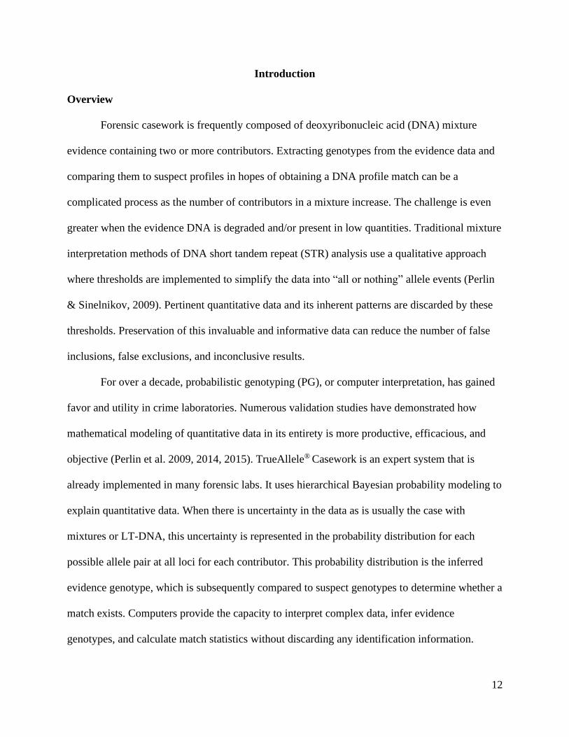
Abstract

Analysis of DNA mixture evidence does not always yield distinct profiles. This process is further

complicated with low template DNA (LT-DNA) samples often seen in forensic casework.

Traditional qualitative methods use thresholds to distinguish allele peaks from stutter peaks,

noise, etc. resulting in data being omitted during analysis. In cases where LT-DNA is present,

low peaks that could potentially be attributed to low contributor profiles may not be called due to

these instituted thresholds. The probabilistic genotyping computer software program created by

Cybergenetics (Pittsburgh, PA), TrueAllele® Casework, considers all data and performs

quantitative analysis using probability to represent uncertainty. It objectively forms likelihood

ratios (LR) that compare the probabilities of an evidentiary genotype with a suspect genotype

relative to a reference population. A joint likelihood function (JLF) takes two or more

independent sets of data and compares them jointly as opposed to a single event. The JLF can

elicit more identification information proving useful in DNA mixture analysis. This project used

TrueAllele® Casework to perform DNA mixture analysis on two sets of previously published

mixture data provided by Cybergenetics. The first set comprised 40 two contributor mixture

samples and the second set included four sets of 10 randomized mixtures with two, three, four,

and five contributors, respectively. The selected samples were interpreted singly and jointly in

three variable groups: mixture weight, template concentration, and complex mixtures. The

differences between the match logLRs of the single and joint analyses were calculated and an

information gain was seen in all three groups when the samples were analyzed jointly. Changing

DNA collection and amplification procedures for touch and DNA mixture evidence samples will

increase the amount of data available for DNA mixture analysis using probabilistic genotyping.

These procedures can be modified so that multiple swabs and replicate amplifications produce

11

more data that TrueAllele can analyze using the JLF. Jointly analyzing each independent

evidence data can lead to higher match statistics which will ultimately help in the identification

of those who commit crimes.

Keywords: DNA mixtures, low template DNA, probabilistic genotyping, likelihood

ratios, joint likelihood function

12

Introduction

Overview

Forensic casework is frequently composed of deoxyribonucleic acid (DNA) mixture

evidence containing two or more contributors. Extracting genotypes from the evidence data and

comparing them to suspect profiles in hopes of obtaining a DNA profile match can be a

complicated process as the number of contributors in a mixture increase. The challenge is even

greater when the evidence DNA is degraded and/or present in low quantities. Traditional mixture

interpretation methods of DNA short tandem repeat (STR) analysis use a qualitative approach

where thresholds are implemented to simplify the data into “all or nothing” allele events (Perlin

& Sinelnikov, 2009). Pertinent quantitative data and its inherent patterns are discarded by these

thresholds. Preservation of this invaluable and informative data can reduce the number of false

inclusions, false exclusions, and inconclusive results.

For over a decade, probabilistic genotyping (PG), or computer interpretation, has gained

favor and utility in crime laboratories. Numerous validation studies have demonstrated how

mathematical modeling of quantitative data in its entirety is more productive, efficacious, and

objective (Perlin et al. 2009, 2014, 2015). TrueAllele® Casework is an expert system that is

already implemented in many forensic labs. It uses hierarchical Bayesian probability modeling to

explain quantitative data. When there is uncertainty in the data as is usually the case with

mixtures or LT-DNA, this uncertainty is represented in the probability distribution for each

possible allele pair at all loci for each contributor. This probability distribution is the inferred

evidence genotype, which is subsequently compared to suspect genotypes to determine whether a

match exists. Computers provide the capacity to interpret complex data, infer evidence

genotypes, and calculate match statistics without discarding any identification information.

13

These tasks can also be performed simultaneously on more than one set of data (Ballantyne et al.,

2013; Perlin et al., 2011).

A joint likelihood function (JLF) takes two or more independent sets of data and

compares them jointly as opposed to a single event. The additional data used in the JLF

constrains the probability distribution for each locus. This in turn, results in higher probabilities

assigned to the allele pairs that provide a good explanation for each set of data. When replicate

amplifications are performed for an evidence item, the STR profiles in each replicate can be

analyzed together with the JLF (Ballantyne et al., 2013). Replicate amplifications are typically

performed on LT-DNA samples to compensate for the increased stochastic effects seen during

PCR which result in allele drop-out, indistinguishable stutter peaks, etc. To account for the

replicate data using manual interpretation, a consensus profile is formed from the data peaks that

are reproduced in two out of three runs. If an allele is seen in only one of the replicates but

dropped out in the other two, it is not considered for the consensus profile (Butler, 2015, Chapter

7). Like the traditional interpretation methods, the consensus approach discards information. PG

methods use all the data and the JLF assigns a probability to those replicates that would

otherwise be discarded. Qualitative approaches can be overwhelmed with additional data

especially when high uncertainty is present. Replicate amplifications and the JLF can potentially

provide more identification information leading to higher match statistics compared to match

statistics from a single amplification. This can prove useful in DNA mixture analysis.

Importance

Increased scrutiny and high public expectations of forensic DNA evidence calls for

accurate, reliable, and efficient DNA mixture interpretation methods. These methods must result

14

in more probative and reliable identification information that can exculpate the innocent and

incriminate those responsible of committing crimes.

This project utilized TrueAllele® Casework to perform DNA mixture analysis and obtain

match statistics in the form of logLR values. This analysis was performed on two sets of

previously published data, varying in mixture weight and DNA quantity, that were provided by

Cybergenetics. The first set comprised 40 two contributor mixture samples and the second set

included two, three, four, and five contributor mixtures. The samples were interpreted singly and

jointly in two ways: in duplicate and triplicate. Mixture weight and template concentration were

two data variables that were considered independently. The data for each variable was analyzed

separately to see how the uncertainty in each would affect the match log LR values obtained

from joint and single analysis. The second set combined varying mixture weights, template

concentrations, and number of contributors. It was demonstrated that replicate amplifications can

result in higher match statistics. This supports the suggestion that DNA collection and

amplification procedures in forensic cases be modified so that more data is available for DNA

mixture analysis using probabilistic genotyping and the JLF.

Background

The use of DNA to uniquely identify an individual in forensic evidence has been a widely

accepted and lauded method to identify perpetrators of violent crimes. A wide array of crime

scene evidence samples is sent to forensic laboratories with hopes of retrieving highly coveted

DNA profiles. Because genetic identity is naturally represented in an individual’s genotype,

identification information is represented in a DNA profile. Because DNA profiles are vital to

criminal justice proceedings, correctly inferring genotypes from evidence DNA using sound

15

scientific and statistical approaches is undoubtedly a delicate and important task. (Perlin,

Kadane, et al., 2009; Perlin & Sinelnikov, 2009; Perlin, 2015).

STR Genotyping

Biological evidence samples are subjected to a multi-step process where DNA is

extracted from the biological specimens, quantified, and amplified via the polymerase chain

reaction (PCR). Only specific non-coding regions of DNA containing short tandem repeats

(STR) are targeted during amplification. These regions are referred to as STR loci or locus if

referring to only one. These STR loci are composed of DNA segments where the sequence

repeats itself. These segments are categorized by the number of base pairs (bp) in the repeating

sequence and the number of repeating units in the locus. The number of repeats at a locus is

given the term allele and a genotype is formed by two alleles at each locus: one passed down

from the father and one from the mother. An individual is said to be homozygous at a locus when

both alleles are the same value. A heterozygous individual has two different alleles. A vast

amount of possible allele combinations exists for every locus which makes STR genotyping

useful for human identification. The STR profile is the composite of these locus genotypes. In

forensic science, commercial STR kits can target more than 20 STR loci that result in different

genotype possibilities for a single individual (Butler, 2010, Chapter 8; Perlin, 2013).

Conversion of biological evidence to DNA begins with extraction. This process involves

the release of DNA from cells, purification of the DNA through washes, and concentration of the

DNA. The DNA is then quantified to assess how much was extracted. A template amount of 0.5

to 1 ng of DNA works best for most STR kits. If enough DNA is available for further processing,

PCR amplification is performed. After PCR, millions of STR fragments are separated via

capillary electrophoresis by size and represented as peaks in an electropherogram (EPG)

16

demonstrated in Figure 1 below (Butler, 2005, Chapters 1-3, 14). Peaks are a visual

representation of DNA quantity and amount of PCR product measured by height in relative

fluorescence units (RFU) and size in base pairs (bp). The amount of DNA present in a sample is

indicated by the peak height. Peaks also represent alleles at each locus. An allele designation

Figure 1

EPG of all loci for reference sample H1

Note. The peaks represent different sized STR fragments.

is given to a peak based on its size. The size of a peak is determined by the number of base pairs

(bp) the STR fragments contain. The greater the number of repeats in an STR fragment, the

bigger the size of the peak. Larger sized alleles contain a greater number of bp and may not

replicate as consistently during PCR leading to smaller amounts of PCR products. Because peak

heights represent PCR product amount, larger sized alleles often have shorter peaks than smaller

sized alleles. This proportionality is affected by DNA template concentration (Butler, 2010,

Appendix 1; Butler, 2015, Chapter 4).

Computer programs make allele designations for every locus which help in determining

an STR profile. DNA analysis and interpretation then compare the evidence and reference STR

17

profiles to each other which can result in a DNA match (Butler, 2010, Chapters 1, 9-10,

Appendix 1; Perlin & Szabady, 2001).

DNA Mixture Interpretation

The last step of forensic DNA typing is interpretation of the STR data. This involves

inferring genotypes from the data. Evidence genotypes are compared to suspect genotypes and if

a match exists, the weight of this evidentiary match must be represented by a statistic (Perlin,

Kadane, et al., 2009; Perlin & Sinelnikov, 2009). Identification information present in the

genotypes is measured by the match statistic.

DNA mixture analysis requires additional steps. First, it must be determined that a

mixture is present. This is accomplished by reviewing the EPG data for every locus. All loci are

assessed for number of peaks, peak heights, and peak height ratios. A peak height ratio (PHR) is

the measurement of the peak height of one allele over the peak height of another allele for a

locus. PHRs are affected by locus size, effectiveness of fragment separation, and DNA template

concentration. When an individual is homozygous at a locus, only one allele peak is present. A

heterozygous individual will have two allele peaks at one locus and how well those alleles

amplified is measured by the PHR. Heterozygous loci with relatively equal peak heights will

have low PHR values. Peak height imbalance occurs when there is a large difference between the

peak heights of heterozygous alleles indicated by a high PHR. A single source sample will

usually produce one or two allele peaks at every locus with low PHR values. If the number of

peaks at a locus is greater than two or the difference in peak height ratios is too great to originate

from a single source (greater than 30%-40%), the STR data indicate the presence of a mixture

(Butler, 2010, Appendix 1; Butler 2015, Chapter 4).

18

The mixture weight of each contributor is determined next. Different amounts of DNA

are contributed by each individual present in a mixture. An individual that has contributed high

quantities of DNA is said to be a major contributor and is identified by tall data peaks. Minor

contributors are represented by shorter peaks indicating lower quantities of their DNA being

present in the mixture. Once it has been determined that more than one contributor is present in a

DNA evidence sample, their weight of contribution can be determined using PHRs (Butler, 2010,

Chapter 10). Obtaining mixture weights for each contributor helps infer contributor genotypes

which can be compared to a reference. If both the evidence and suspect genotypes match, a

match statistic can be calculated, and the amount of identification information determined.

Though simple in theory, DNA mixture analysis is known to be an intricate and difficult process.

Single source samples usually provide clean and ideal data which makes DNA analysis of

these samples a straightforward task. This is not usually the case for STR profiles derived from

crime scene evidence. DNA evidence from crime scenes can be low template, damaged, or a

mixture of two or more individuals. When evidence of this nature is amplified, it can result in

low peak heights, missing peaks, or several peaks indicative of a mixture. Low peak heights

indicate low quantities of DNA which can lead to peak height imbalance at heterozygous loci. If

damage to the DNA is extensive, there will be regions in the DNA that will not amplify during

PCR. This results in allele drop-out, an extreme form of peak height imbalance. When more than

two contributors are present in a mixture, the amount of DNA present for each can vary

potentially resulting in low peak heights and peak height imbalance between major and minor

contributors. Each of these elements in isolation or combined, makes it difficult to confidently

infer locus genotypes. This results in uncertainty in the data, the inferred genotypes, and the

resulting match statistics (Ballantyne et al, 2013; Perlin et al., 2011).

19

The goal of qualitative and quantitative mixture interpretation methods is to address data

uncertainty. Qualitative methods implement thresholds to address uncertainty but in doing so,

discard data peaks that can be useful in determining genotypes if they fall below the threshold

(Greenspoon et al., 2015). Figure 2 provides a visual example of how thresholds can discard

information at a locus. This decreases the identification information of a subsequent match

statistic. Perlin and Sinelnikov (2009) determined that qualitative mixture interpretation methods

are less informative than quantitative methods. This is due to the utilization of all the available

data by quantitative methods. The variation present in the data is mathematically accounted for

by assigning probabilities to all possible genotypes at each locus (Bauer et al., 2020; Gill et al.,

2012; Perlin et al., 2014). Probabilities are used to explain the data peak patterns and preserve

identification information.

Figure 2

EPG of TPOX for sample J4

Note. The analytical threshold (AT) is set to 50 RFUs.

20

Interpretation of STR data culminates in the comparison of an evidence genotype with a

reference genotype to see if a match is obtained. There are different approaches to calculate a

match statistic, but quantitative approaches use likelihood ratios (LR) which account for

probabilities. An LR “is a calculation of the ratio of probabilities of observing the DNA under

two alternative hypotheses” (Gill et al., 2012). These hypotheses are commonly referred to as the

prosecutor’s hypothesis and the alternative or defense hypothesis. The prosecutor’s hypothesis

assumes that the suspect did contribute their DNA to the evidence while the alternative

hypothesis is that some other unrelated individual contributed their DNA to the evidence. When

the LR is greater than one, it supports the hypothesis that the suspect contributed to the evidence.

If the LR is less than one, support for the alternative hypothesis strengthens. The base 10

logarithm of the LR, logLR, is used to measure the change of information in the evidence, show

how well the data preserves identification information, and can be expressed in ban units (Good,

1979, as cited in Ballantyne et al., 2013). The match logLR weighs the strength of the

relationship between the evidence genotype and suspect genotype relative to a population.

Because quantitative methods utilize all the available data in an STR profile and objectively infer

evidence genotypes, preservation of identification information is captured best in the match

logLR obtained from probabilistic genotyping (Perlin et al., 2014). How informative the match

logLR is then measured by its value which also indicates how much identification information

was preserved from the quantitative data. In criminal proceedings, LR match statistics that reach

or surpass 6 ban (one in a million) tend to have the most persuasive effect on juries, but the

method used to calculate the match logLR should also be an indicator of how informative and

reliable a match statistic is (Koehler, 2001, as cited in Perlin & Sinelnikov, 2009). TrueAllele

computes this match statistic using all the identification information present in the data.

21

TrueAllele® Casework

TrueAllele® Casework is a software program that uses a hierarchical Bayesian model to

explain STR data and infer genotypes. The likelihood function (LF) in Bayes theorem accounts

for genotype, mixture weight, PCR stutter, relative amplification, and DNA degradation that may

be present in the data using the peak height variation and mixture variation between different loci

(Perlin et al., 2011). A statistical search of the STR data using Markov chain Monte Carlo

(MCMC) is conducted by the computer which tries different variable combinations to explain the

data. Thousands of MCMC cycles sequentially test these variables using new combinations each

cycle. The combinations that give a better explanation for the data are assigned a higher

likelihood (giving higher probability values) and a lower likelihood is given to the pairs whose

explanation is poor (leading to lower probability for the combination). The result is a posterior

probability distribution for all allele pairs at every locus for each contributor from which

genotypes are inferred. A match LR, expressed as a logLR, is calculated when the inferred

evidence genotypes are compared to a reference genotype from a particular individual relative to

a population. Because TrueAllele uses all the quantitative data available for interpretation, the

match logLR is a reliable number conveying a sample’s identification information (Ballantyne et

al., 2013; Greenspoon et al., 2015; Perlin et al., 2011; Perlin et al., 2015; Perlin & Sinelnikov,

2009).

Independent sets of data can be analyzed and multiplied together using a joint likelihood

function (JLF). The probabilities that result for each independent data set are multiplied together

using the JLF which increases the posterior probability distribution of the locus allele pairings.

When there is high uncertainty in STR data as seen with LT-DNA and mixtures, the posterior

probability distribution will be diffuse for allele pairings across all loci. A diffuse probability is

22

indicative of uncertainty and will result in a lower match statistic. Joint interpretation of multiple

data sets can lead to higher probabilities because the additional data is constrained by the

variable combinations that give the best explanation jointly during MCMC sampling. A JLF can

help tighten and increase those probability distributions if LT-DNA and mixture samples are

amplified in replicates and interpreted jointly (Perlin, Kadane, et al., 2009). Replicate

amplification of evidence highly suspected to contain LT-DNA or consist of a mixture, will

provide a greater amount of data that TrueAllele can readily process. By applying the JLF,

higher probabilities will naturally result in higher and more informative match statistics for

replicates that come from the same piece of evidence or evidentiary material that are closely

related.

Review of Literature

TrueAllele uses probabilistic modeling (Bayes theorem) and statistical sampling

(MCMC) methods that have been established for decades and are used by different disciplines

such as “nuclear physics, psychology, computer learning, economics, biological systems, and

more recently, DNA analysis” to explain complex data patterns (Greenspoon et al., 2015). It has

been established that mathematical modeling of complex evidence mixture data has produced

consistently higher match statistics compared to manual review. Computer interpretation has

proven to be objective, efficient, and reproducible in several studies. Perlin et al. (2009, 2011,

2013, 2014, 2015) have performed validation studies using Cybergenetics TrueAllele® Casework

for mixture interpretation. Interpretation was performed on data obtained from premixed

templates from the National Institute of Standards and Technology (NIST), adjudicated cases

from the New York State Police Forensic Investigation Center (Perlin et al., 2011, 2013),

mixture evidence in 72 cases from the Virginia Department of Forensic Science, and data created

23

by Sorenson Forensics for the Kern County Regional Crime Laboratory in these particular

validation studies, respectively. The studies compared the traditional qualitative methods of

inclusion probability and combined probability of inclusion to TrueAllele interpretation and

concluded that TrueAllele preserved the most identification information. The preservation of

identification information by TrueAllele has supported its use in criminal cases.

TrueAllele has been officially used in forensic casework since 2009 and it has been

instrumental in many criminal trials such as Commonwealth of Pennsylvania v. Kevin J. Foley

and Commonwealth of Pennsylvania v. Glenn Lyons. The United Kingdom (UK) has also used

TrueAllele. Match statistics calculated by TrueAllele were pivotal in the case of the Queen v.

Duffy & Shivers where Brian Shivers was convicted of murdering two soldiers who died in the

2009 terrorist attack of the Massereene Barracks in Northern Ireland (Perlin, 2013, 2015; Perlin

& Galloway, 2012; Perlin & Sinelnikov, 2009). TrueAllele has also been used to identify victims

from the World Trade Center disaster and in building the UK’s National DNA Database. Crime

labs in California, Louisiana, Maryland, South Carolina, Ohio, Georgia, and Virginia have

already incorporated TrueAllele into their DNA analysis process (Bauer et al., 2020; Kwong,

2017).

Because previous validation studies established the reliability and objectivity of

probabilistic genotyping and TrueAllele is already used in forensic casework, it is important to

explore other applications of computer modeling in mixture interpretation. An earlier study by

Ballantyne et al. (2013) looked at how a JLF can increase identification information with

samples varying in mixture weight. Mixture weight is the measurement of how much template

DNA was contributed to the sample by a single contributor to the mixture. (Perlin & Szabady,

2001). Peak height imbalance helps distinguish one contributor from another but when a mixture

24

contains equal contributor weights, the peak heights are also relatively equal. Equal weighted

mixtures increase uncertainty in the inferred genotypes leading to a decrease in identification

information. Ballantayne et al.’s 2013 study used binomial sampling of an equal weighted

mixture to produce sub-samples containing different mixture weights to elicit more identification

information. Several sample groupings were analyzed using the data from a single experiment,

but two experiments were combined and analyzed using a JLF. TrueAllele was used to jointly

analyze the two sets of data to test the hypothesis that joint analysis of multiple experiments will

increase identification information. This study found that pairing one experiment with another

generally increased identification information. Even though there were instances where no

increase was seen and even a decrease occurred, the full sample genotype information was

recovered using the joint likelihood thus preserving and increasing identification information.

The study concluded by suggesting that using joint likelihoods with samples varying in mixture

weight can obtain greater identification information in routine casework as well. Variations in

mixture weight can be generated with “micro-geographical samplings” of physiological stain

evidence and creation of sub-samples from limited dilutions of DNA extract of mixture evidence

(Ballantyne et al., 2013). The resulting data from these sub-samples created from casework

evidence can be interpreted jointly using TrueAllele resulting in more genetic information.

Materials and Methods

Materials

• TrueAllele® Casework

• TrueAllele® Visual User Interface (VUIer™)

• TrueAllele® VUIer™ manuals for Analyze, Data, Request, Review, and Report modules

• Microsoft Excel

25

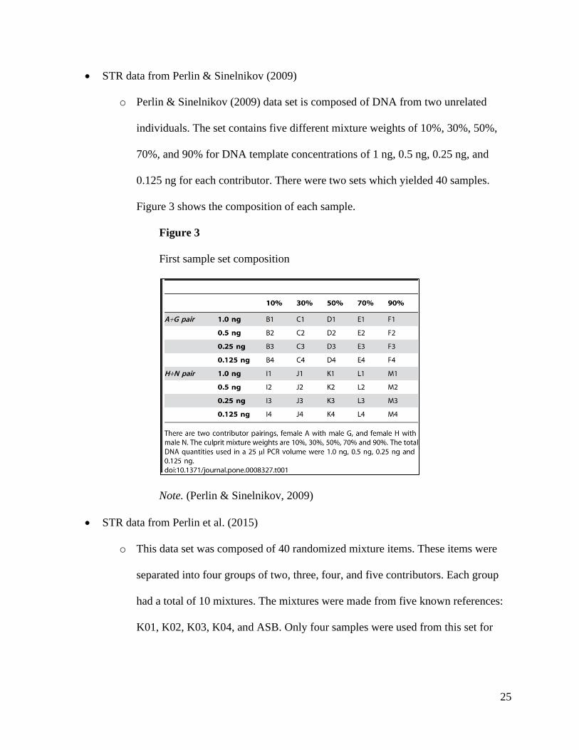
• STR data from Perlin & Sinelnikov (2009)

o Perlin & Sinelnikov (2009) data set is composed of DNA from two unrelated

individuals. The set contains five different mixture weights of 10%, 30%, 50%,

70%, and 90% for DNA template concentrations of 1 ng, 0.5 ng, 0.25 ng, and

0.125 ng for each contributor. There were two sets which yielded 40 samples.

Figure 3 shows the composition of each sample.

Figure 3

First sample set composition

Note. (Perlin & Sinelnikov, 2009)

• STR data from Perlin et al. (2015)

o This data set was composed of 40 randomized mixture items. These items were

separated into four groups of two, three, four, and five contributors. Each group

had a total of 10 mixtures. The mixtures were made from five known references:

K01, K02, K03, K04, and ASB. Only four samples were used from this set for

26

analysis: mixtures 1.1, 2.8, 3.6, and 4.2. References K01 and ASB were present in

all four samples.

Methods

After computer installation of TrueAllele® Casework and TrueAllele® VUIer™,

familiarization with the manuals, and completion of the tutorial material, data for analysis was

selected considering two common sources of data uncertainty: mixture weight and template

concentration. Using the data from Perlin & Sinelnikov (2009), mixture weight and template

concentration were considered as separate variables to see which elicited more information using

the JLF. A second data set (Perlin et al., 2015) involved more complex mixtures which varied in

mixture weight, template concentration, and number of contributors. All three variables of the

second data set were intertwined in the joint analysis.

In order to observe how well a JLF recovers identification information from varying

mixture weights, the 1 ng template samples were used from the Perlin & Sinelnikov (2009) data

in different mixture weight combinations. Table 1 shows these combinations. Each sample was

analyzed independently using TrueAllele® Casework. Then the samples were combined in

duplicate and triplicate for joint analysis. This same pattern was also used for the low template

samples.

Table 1

Mixture Weight Combinations for Single and Joint Interpretation

References A1 and G1 References H1 and N1

Mixture Weight

Single Duplicate Triplicate Single Duplicate Triplicate

0.9/0.1 B1 B1+D1 B1+C1+D1 I1 I1+K1 I1+J1+K1

0.7/0.3 C1 C1+D1 D1+E1+F1 J1 J1+K1 K1+L1+M1

0.5/0.5 D1 B1+C1 K1 I1+J1

27

References A1 and G1 References H1 and N1

Mixture Weight

Single Duplicate Triplicate Single Duplicate Triplicate

0.3/0.7 E1 D1+E1 L1 K1+L1

0.1/0.9 F1 D1+F1 M1 K1+M1

E1+F1 L1+M1

Note. Mixture weight is indicated for the single samples.

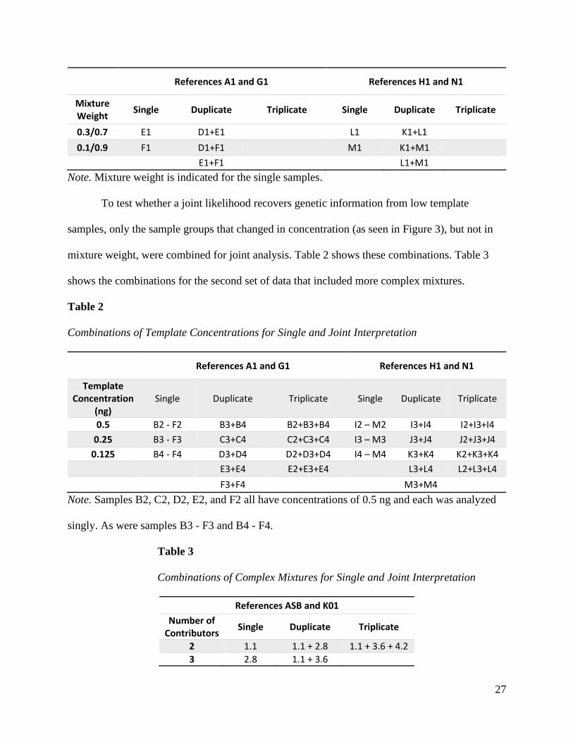
To test whether a joint likelihood recovers genetic information from low template

samples, only the sample groups that changed in concentration (as seen in Figure 3), but not in

mixture weight, were combined for joint analysis. Table 2 shows these combinations. Table 3

shows the combinations for the second set of data that included more complex mixtures.

Table 2

Combinations of Template Concentrations for Single and Joint Interpretation

References A1 and G1 References H1 and N1

Template Concentration

(ng) Single Duplicate Triplicate Single Duplicate Triplicate

0.5 B2 - F2 B3+B4 B2+B3+B4 I2 – M2 I3+I4 I2+I3+I4

0.25 B3 - F3 C3+C4 C2+C3+C4 I3 – M3 J3+J4 J2+J3+J4

0.125 B4 - F4 D3+D4 D2+D3+D4 I4 – M4 K3+K4 K2+K3+K4

E3+E4 E2+E3+E4 L3+L4 L2+L3+L4

F3+F4 M3+M4

Note. Samples B2, C2, D2, E2, and F2 all have concentrations of 0.5 ng and each was analyzed

singly. As were samples B3 - F3 and B4 - F4.

Table 3

Combinations of Complex Mixtures for Single and Joint Interpretation

References ASB and K01

Number of Contributors

Single Duplicate Triplicate

2 1.1 1.1 + 2.8 1.1 + 3.6 + 4.2

3 2.8 1.1 + 3.6

28

References ASB and K01

Number of Contributors

Single Duplicate Triplicate

4 3.6 1.1 + 4.2

5 4.2 3.6 + 4.2

Note. The number of contributors is indicated for the single samples.

TrueAllele® Casework Visual User Interface (VUIer™) contains six modules where

different steps of the interpretation and analysis process are performed: Analyze, Data, Request,

Review, Report, and Tools. The Data, Request, Review, and Report modules were primarily

used for this research. The STR data files from Perlin & Sinelnikov (2009) and Perlin et al.

(2015) were stored in a TrueAllele World, a database where files and interpretation requests are

stored, from which they were accessed for subsequent analysis (Hornyak et al., 2015).

The Data module was used to access the TrueAllele World that contained the two sets of

previously published data. The STR data files were downloaded and used to form interpretation

requests for each single sample, duplicate combination, and triplicate combination for mixture

weight, template concentration, and complex mixtures groups in the Request module. Each

interpretation request indicated the maximum number of contributors for each sample being

analyzed. The requests were reviewed and uploaded to a cloud server where they were

processed.

TrueAllele uses MCMC statistical searching where different variables (genotype, mixture

weight, etc.) are used to try to explain the STR data and separate the contributors in a mixture.

Contributor genotypes are inferred from the probability distributions determined for each

variable during MCMC sampling. The number of times the computer will subject the data to

MCMC sampling is determined by the number entered for burn-in and read-out cycles in the

Request module (Greenspoon et al., 2015; Hornyak et al., 2015; Perlin et al., 2011, 2013). The

time it takes for an interpretation request to process depends on the number of cycles used for

29

each request. A high number of cycles will usually result in more information but will also lead

to longer running times. Fewer cycles lead to shorter running times. When data is known to be

complex and high uncertainty is expected, a greater number of burn-in and read-out cycles are

used. Single source data or simple mixtures can be processed with lower cycle settings. The

number of cycles that can be chosen vary from 5,000 (5K), 10,000 (10K), 25,000 (25K), 50K,

100K, and 250K.

The samples in Tables 1 and 2 were analyzed using 5K burn-in and read-out cycles.

Because this first set of data was composed of simple two contributor mixtures with known

concentrations and mixture weights, the number of cycles was kept at 5K. The set of complex

mixtures in Table 3 were analyzed using 50K cycles to account for the higher degree of

variability in the data. All the requests were run once except for the following: D3, C4, D4, L3,

J4, D3+D4, L3+L4, and F2+F3+F4. Initial run results for these samples deviated slightly in their

inferred mixture weights compared to their original design and results from the previous studies

and analyses performed on the same data in Perlin & Sinelnikov (2009). The averages of both

runs were used, and the second run results were used for D3+D4.

Once the interpretation requests were done processing, the Review module was used to

check the locus probability distributions for each set. The match logLR results for each

interpretation request were obtained in the Report module. The inferred genotypes for each

request were selected and compared to the references in the sample mixture relative to a random

population. The NIST1036_2017_ALL was the population database chosen for this research

which contains allele frequencies for the Caucasian, African American, Asian, and Hispanic

population groups used to calculate match statistics (National Institute for Standards and

Technology, 2014). Each comparison was broken down by sample, contributor, number of

30

contributors, weight of each contributor, the standard deviation, the KL (Kullback-Leibler)

statistic, and the match logLR values for each reference. The evidence sample, designed mixture

weight of each contributor, and the match logLR values are presented in tables below.

Data Analysis and Interpretation

The match logLRs obtained from each interpretation request were grouped by single,

duplicate, and triplicate analysis for each variable group. Results from samples B-F and I-K

showed a change in logLRs for single and joint analyses. The results for samples I-K are shown

here to display the change in match information for 50/50 mixture weights, minor contributors,

and low template concentrations. Tables 4-6 display mixture weight combinations, Tables 7-9

display LT-DNA results, and Table 10-11 contain results for complex mixtures.

Mixture Weight Comparison

Mixture weights (MW) are calculated by summing the peak height values of the minor

peaks and dividing that value by the sum of all peaks at a locus. Manual calculations use only the

loci where major and minor contributor peaks are distinguishable. TrueAllele and PG software

can calculate the weights for all loci (Greenspoon et al., 2015; Perlin et al., 2013). Many studies

state that equal weighted mixtures result in lower and more diffuse probabilities. Because each

possible allele pair combination will be equally likely with similar sized peaks, the probability

distribution will decrease in 50/50 mixtures. Ballantyne et al. (2013) claim that mixtures where

two individuals have contributed an approximate equal amount of DNA are some of the most

challenging because there are no distinct major and minor peaks. Differences in peak heights

help attribute which contributor goes with which genotype thus increasing the identification

information (Perlin et al., 2013, 2015; Perlin & Sinelnikov, 2009). Different mixture weight

31

combinations were analyzed to compare what mixture weight variations gained more

identification information in the match logLR when interpreted jointly.

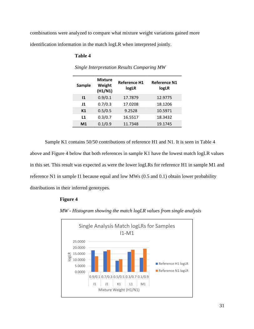
Table 4

Single Interpretation Results Comparing MW

Sample Mixture Weight (H1/N1)

Reference H1 logLR

Reference N1 logLR

I1 0.9/0.1 17.7879 12.9775

J1 0.7/0.3 17.0208 18.1206

K1 0.5/0.5 9.2528 10.5971

L1 0.3/0.7 16.5517 18.3432

M1 0.1/0.9 11.7348 19.1745

Sample K1 contains 50/50 contributions of reference H1 and N1. It is seen in Table 4

above and Figure 4 below that both references in sample K1 have the lowest match logLR values

in this set. This result was expected as were the lower logLRs for reference H1 in sample M1 and

reference N1 in sample I1 because equal and low MWs (0.5 and 0.1) obtain lower probability

distributions in their inferred genotypes.

Figure 4

MW - Histogram showing the match logLR values from single analysis

0.0000

5.0000

10.0000

15.0000

20.0000

25.0000

0.9/0.1 0.7/0.3 0.5/0.5 0.3/0.7 0.1/0.9

I1 J1 K1 L1 M1

logL

R

Mixture Weight (H1/N1)

Single Analysis Match logLRs for Samples I1-M1

Reference H1 logLR

Reference N1 logLR

32

Table 5

Duplicate Interpretation Results Comparing MW

Sample Mixture Weight (H1/N1)

Reference H1 logLR

Reference N1 logLR

I1+K1 0.9/0.1

+ 0.5/0.5

17.7879 19.1727

J1+K1 0.7/0.3

+ 0.5/0.5

17.6994 19.0926

I1+J1 0.9/0.1

+ 0.7/0.3

17.7879 19.0615

K1+L1 0.5/0.5

+ 0.3/0.7

17.7584 19.1468

K1+M1 0.5/0.5

+ 0.1/0.9

17.7812 19.1745

L1+M1 0.3/0.7

+ 0.1/0.9

17.4381 19.1745

Table 5 above displays the logLRs for the duplicate combinations. It can be noticed

immediately that an information gain was observed for each reference in each duplicate as

compared to the single analyses shown in table 4. The logLR values for I1+K1 and I1+J1 were

equal at 17.7879 ban. This can occur when the probability is practically near or equal to 100%

for evidence genotype allele pairs meaning that all the probability is concentrated on the

reference allele pairs. When the same population database is used for the match logLR

calculation, a maximum value is obtained because the LR calculation changes from uncertain

probability divided by the population at the reference allele pair to one divided by the population

genotype. Reference H1 in sample I1 has a weight of 0.9 or 90% as does reference N1 in sample

M1indicating that probability is concentrated on the allele pairs of these references in the

33

duplicate and triplicate joint analyses. Duplicates and triplicates containing references whose

weights are 90% have logLR values that are equal or close to equal indicating that high mixture

weights whose probability is close to 100% “maxes out” a match logLR value.

Table 6

Triplicate Interpretation Results Comparing MW

Sample Mixture Weight (H1/N1)

Reference H1 logLR

Reference N1 logLR

I1+J1+K1

0.9/0.1 +

0.7/0.3 +

0.5/0.5

17.7879 19.1732

K1+L1+M1

0.5/0.5 +

0.3/0.7 +

0.1/0.9

17.7879 19.1745

Triplicate analysis showed little to no change compared to duplicate analysis but a gain

was demonstrated in triplicate analysis compared to single analysis. Some logLR values in Table

5 and 6 are equal or close to equal. When the quantity of DNA is high and the inferred genotype

probability distribution is near or reaches 100% probability, the major contributor’s logLR value

ceases to increase and stays relatively constant at its maximum value (Bauer et al., 2020). Minor

contributors can have their logLR values display this trend as well.

LT-DNA Comparison

After DNA extraction is performed, the quantity of DNA present in the evidence is

determined. Quantities of 0.2 ng and lower are deemed low template (Butler, 2010, Chapter 14,

18). The stochastic effects of PCR are exacerbated as DNA quantities decrease leading to greater

34

occurrences of peak height imbalance, allele drop-out, stutter, etc. This results in heightened

uncertainty, lower probability distributions, and lower match statistics for LT-DNA samples.

The proportional relationship between DNA weight contribution and logLR values

dictates that as the amount of DNA contributed increases so does the logLR for major and minor

contributors. The opposite is also observed. When the amount of DNA weight decreases so does

the logLR (Bauer et al., 2020; Perlin & Sinelnikov, 2009). When a mixture sample is low

template, minor contributors with exceptionally low mixture weights have even lower amounts

of DNA present in the sample resulting in extremely low and uninformative logLRs. This trend

is displayed in these results. The results of the single analyses for samples at the lowest template

concentrations of 0.125 ng in the first data set are shown in Table 7. Though the concentrations

are constant for samples I4-M4, each sample has a different mixture weight. It can be observed

that as weight decreases, logLR values rapidly decrease as well at low template concentrations.

Negative logLRs were even observed. Greater gains in identification information are seen for

low template samples when analyzed jointly.

Table 7

Results from Single Interpretation of LT-DNA Samples

Sample

(0.125 ng)

Target Weight (H1/N1)

Reference H1 logLR

Reference N1 logLR

I4 0.9/0.1 17.4153 1.9852

J4 0.7/0.3 8.6165 6.0900

K4 0.5/0.5 8.0504 8.4280

L4 0.3/0.7 -0.4628 13.7580

M4 0.1/0.9 -0.4874 18.2591

35

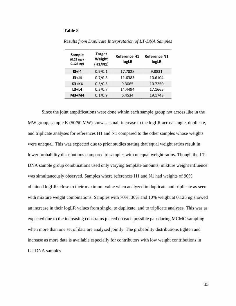
Table 8

Results from Duplicate Interpretation of LT-DNA Samples

Sample

(0.25 ng + 0.125 ng)

Target Weight (H1/N1)

Reference H1 logLR

Reference N1 logLR

I3+I4 0.9/0.1 17.7828 9.8831

J3+J4 0.7/0.3 11.6383 10.6104

K3+K4 0.5/0.5 9.3065 10.7250

L3+L4 0.3/0.7 14.4494 17.1665

M3+M4 0.1/0.9 6.4534 19.1743

Since the joint amplifications were done within each sample group not across like in the

MW group, sample K (50/50 MW) shows a small increase to the logLR across single, duplicate,

and triplicate analyses for references H1 and N1 compared to the other samples whose weights

were unequal. This was expected due to prior studies stating that equal weight ratios result in

lower probability distributions compared to samples with unequal weight ratios. Though the LT-

DNA sample group combinations used only varying template amounts, mixture weight influence

was simultaneously observed. Samples where references H1 and N1 had weights of 90%

obtained logLRs close to their maximum value when analyzed in duplicate and triplicate as seen

with mixture weight combinations. Samples with 70%, 30% and 10% weight at 0.125 ng showed

an increase in their logLR values from single, to duplicate, and to triplicate analyses. This was as

expected due to the increasing constrains placed on each possible pair during MCMC sampling

when more than one set of data are analyzed jointly. The probability distributions tighten and

increase as more data is available especially for contributors with low weight contributions in

LT-DNA samples.

36

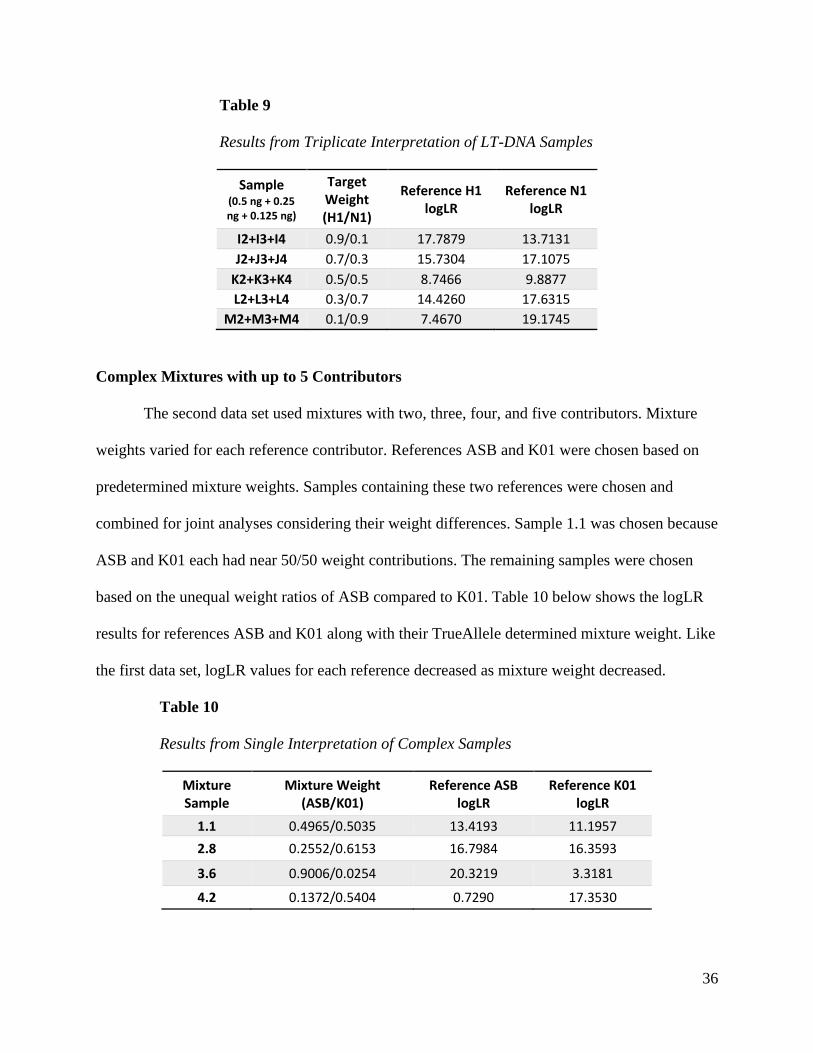
Table 9

Results from Triplicate Interpretation of LT-DNA Samples

Sample (0.5 ng + 0.25 ng + 0.125 ng)

Target Weight (H1/N1)

Reference H1 logLR

Reference N1 logLR

I2+I3+I4 0.9/0.1 17.7879 13.7131

J2+J3+J4 0.7/0.3 15.7304 17.1075

K2+K3+K4 0.5/0.5 8.7466 9.8877

L2+L3+L4 0.3/0.7 14.4260 17.6315

M2+M3+M4 0.1/0.9 7.4670 19.1745

Complex Mixtures with up to 5 Contributors

The second data set used mixtures with two, three, four, and five contributors. Mixture

weights varied for each reference contributor. References ASB and K01 were chosen based on

predetermined mixture weights. Samples containing these two references were chosen and

combined for joint analyses considering their weight differences. Sample 1.1 was chosen because

ASB and K01 each had near 50/50 weight contributions. The remaining samples were chosen

based on the unequal weight ratios of ASB compared to K01. Table 10 below shows the logLR

results for references ASB and K01 along with their TrueAllele determined mixture weight. Like

the first data set, logLR values for each reference decreased as mixture weight decreased.

Table 10

Results from Single Interpretation of Complex Samples

Mixture Sample

Mixture Weight (ASB/K01)

Reference ASB logLR

Reference K01 logLR

1.1 0.4965/0.5035 13.4193 11.1957

2.8 0.2552/0.6153 16.7984 16.3593

3.6 0.9006/0.0254 20.3219 3.3181

4.2 0.1372/0.5404 0.7290 17.3530

37

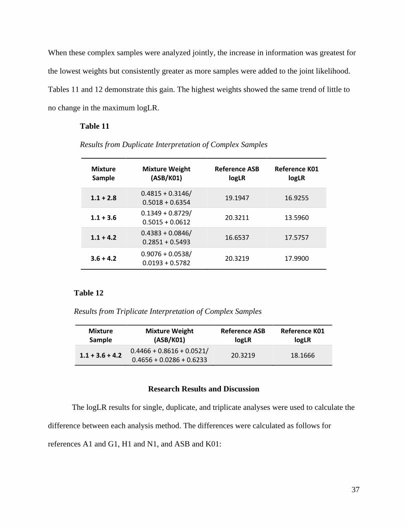
When these complex samples were analyzed jointly, the increase in information was greatest for

the lowest weights but consistently greater as more samples were added to the joint likelihood.

Tables 11 and 12 demonstrate this gain. The highest weights showed the same trend of little to

no change in the maximum logLR.

Table 11

Results from Duplicate Interpretation of Complex Samples

Mixture Sample

Mixture Weight (ASB/K01)

Reference ASB logLR

Reference K01 logLR

1.1 + 2.8 0.4815 + 0.3146/ 0.5018 + 0.6354

19.1947 16.9255

1.1 + 3.6 0.1349 + 0.8729/ 0.5015 + 0.0612

20.3211 13.5960

1.1 + 4.2 0.4383 + 0.0846/ 0.2851 + 0.5493

16.6537 17.5757

3.6 + 4.2 0.9076 + 0.0538/ 0.0193 + 0.5782

20.3219 17.9900

Table 12

Results from Triplicate Interpretation of Complex Samples

Mixture Sample

Mixture Weight (ASB/K01)

Reference ASB logLR

Reference K01 logLR

1.1 + 3.6 + 4.2 0.4466 + 0.8616 + 0.0521/ 0.4656 + 0.0286 + 0.6233

20.3219 18.1666

Research Results and Discussion

The logLR results for single, duplicate, and triplicate analyses were used to calculate the

difference between each analysis method. The differences were calculated as follows for

references A1 and G1, H1 and N1, and ASB and K01:

38

Duplicate log LR - single log LR

Triplicate log LR - single log LR

Triplicate log LR - duplicate log LR

These calculations were made for all three variables of mixture weight, low template

concentration, and complex mixtures. The resulting values indicate how much information was

either gained or lost when performing joint analysis of multiple data samples using the JLF.

Mixture Weight

The difference calculations were performed for each sample group. The information gain

or loss across each sample for mixture weight was consolidated for each reference shown

numerically in Tables 14-17. Table 13 shows the log LR values across all three analysis methods

for sample K1. Figures 5-8 visually represent this gain in histograms.

Table 13

Interpretation Results for Sample K1 Using Varied MW Combinations

Sample Target Weight (H1/N1)

Reference H1 logLR

Reference N1 logLR

Information Gain/Loss

H1

Information Gain/Loss

N1

K1 0.5/0.5 9.2528 10.5971

I1+K1 0.9/0.1

+ 0.5/0.5

17.7879 19.1727 8.5351 8.5756

J1+K1 0.7/0.3

+ 0.5/0.5

17.6994 19.0926 8.4466 8.4955

K1+L1 0.5/0.5

+ 0.3/0.7

17.7584 19.1468 8.5056 8.5497

K1+M1 0.5/0.5

+ 0.1/0.9

17.7812 19.1745 8.5284 8.5774

I1+J1+K1

0.9/0.1 +

0.7/0.3 +

17.7879 19.1732 8.5351 8.5761

39

Sample Target Weight (H1/N1)

Reference H1 logLR

Reference N1 logLR

Information Gain/Loss

H1

Information Gain/Loss

N1

0.5/0.5

K1+L1+M1

0.5/0.5 +

0.3/0.7 +

0.1/0.9

17.7879 19.1745 8.5351 8.5774

Table 14

MW - Difference of Single and Joint Analysis for Reference A1

A1 Samples

Target Weight

Dup-single Trip-single Trip-Dup

B 0.9 0.0006 0.0006 0.0000

C 0.7 1.4820 1.4829 0.0009

D 0.5 15.7077 15.7084 0.0007

E 0.3 -0.2148 0.1107 0.3256

F 0.1 6.8666 7.1925 0.3259

Sample K1 gains identification information by approximately 8.5 ban using joint analysis

shown in Table 13. As previously mentioned, the sample containing the higher mixture weight

provided a higher logLR which eventually plateaued between duplicate and triplicate analysis

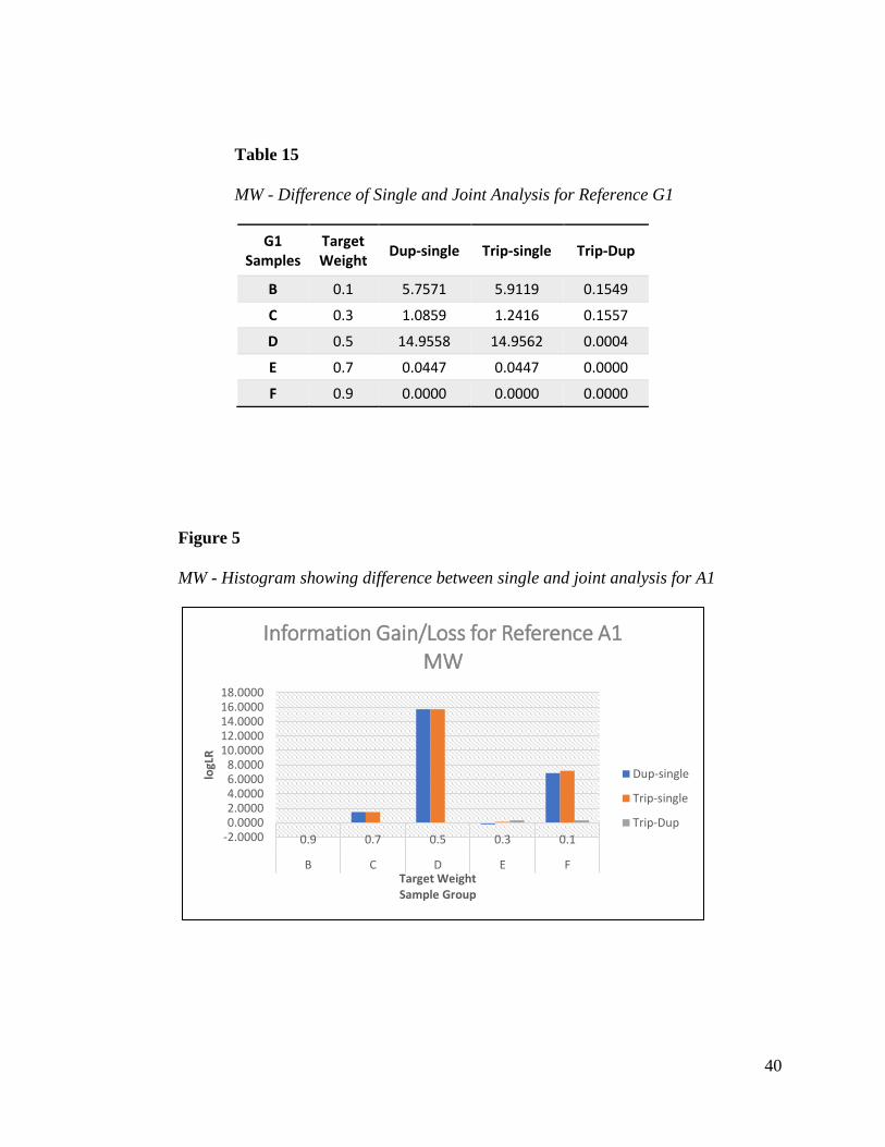
methods. Tables 14 and 15 show that the greatest information gain for references A1 and G1

were seen when their weight contributions were 50% where information increased by 15.7 ban in

A1 and close to 15 ban in G1. When references had a low weight contribution of 10%, gain in

information was also seen. As mixture weight increased, the gain in information was negligible.

The trend is clearly demonstrated in the histograms for each reference.

40

Table 15

MW - Difference of Single and Joint Analysis for Reference G1

G1 Samples

Target Weight

Dup-single Trip-single Trip-Dup

B 0.1 5.7571 5.9119 0.1549

C 0.3 1.0859 1.2416 0.1557

D 0.5 14.9558 14.9562 0.0004

E 0.7 0.0447 0.0447 0.0000

F 0.9 0.0000 0.0000 0.0000

Figure 5

MW - Histogram showing difference between single and joint analysis for A1

-2.00000.00002.00004.00006.00008.0000

10.000012.000014.000016.000018.0000

0.9 0.7 0.5 0.3 0.1

B C D E F

logL

R

Target WeightSample Group

Information Gain/Loss for Reference A1MW

Dup-single

Trip-single

Trip-Dup

41

Figure 6

MW - Histogram showing difference between single and joint analysis for G1

Table 16

MW - Difference of Single and Joint Analysis for Reference H1

H1 Samples

Target Weight

Dup-single Trip-single Trip-Dup

I 0.9 0.0000 0.0000 0.0000

J 0.7 0.7228 0.7671 0.0442

K 0.5 8.5039 8.5351 0.0312

L 0.3 1.0466 1.2362 0.1897

M 0.1 5.8749 6.0531 0.1783

0.00002.00004.00006.00008.0000

10.000012.000014.000016.0000

0.1 0.3 0.5 0.7 0.9

B C D E F

logL

R

Target WeightSample Group

Information Gain/Loss for Reference G1MW

Dup-single

Trip-single

Trip-Dup

42

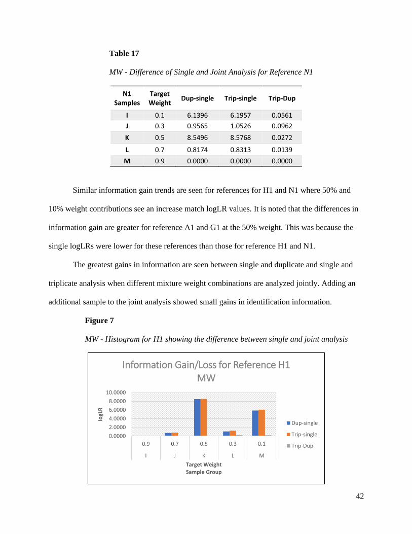
Table 17

MW - Difference of Single and Joint Analysis for Reference N1

N1 Samples

Target Weight

Dup-single Trip-single Trip-Dup

I 0.1 6.1396 6.1957 0.0561

J 0.3 0.9565 1.0526 0.0962

K 0.5 8.5496 8.5768 0.0272

L 0.7 0.8174 0.8313 0.0139

M 0.9 0.0000 0.0000 0.0000

Similar information gain trends are seen for references for H1 and N1 where 50% and

10% weight contributions see an increase match logLR values. It is noted that the differences in

information gain are greater for reference A1 and G1 at the 50% weight. This was because the

single logLRs were lower for these references than those for reference H1 and N1.

The greatest gains in information are seen between single and duplicate and single and

triplicate analysis when different mixture weight combinations are analyzed jointly. Adding an

additional sample to the joint analysis showed small gains in identification information.

Figure 7

MW - Histogram for H1 showing the difference between single and joint analysis

0.0000

2.0000

4.0000

6.0000

8.0000

10.0000

0.9 0.7 0.5 0.3 0.1

I J K L M

logL

R

Target WeightSample Group

Information Gain/Loss for Reference H1MW

Dup-single

Trip-single

Trip-Dup

43

Figure 8

MW - Histogram for N1 showing the difference between single and joint analysis

LT-DNA

Information gain using joint analysis was consistently obtained for the minor contributor

in low template samples for each sample group. The major contributor at the same template

concentration also saw gains but not to the same extent. When using mixture weight as a

variable, there was little difference between the duplicate and triplicate logLRs. Here, the gain is

incremental when analyzing LT-DNA samples jointly as seen for reference N1 in sample I.

Table 18

Difference Between Single and Joint Analysis Results for LT-DNA Sample I4

Sample Template

Concentration (ng)

TA Weight (H1/N1) Reference H1 logLR

Reference N1 logLR

Information Gain/Loss

H1

Information Gain/Loss

N1

I4 0.125 0.9132/0.0868 17.4153 1.9852

I3+I4 0.25 + 0.125 0.8714 + 0.9087/ 0.1286 + 0.0913

17.7828 9.8831 0.3675 7.8979

I2+I3+I4 0.5 + 0.25+

0.125 0.8872 + 0.8670 + 0.8618/ 0.1128 + 0.1330 + 0.1382

17.7879 13.7131 0.3726 11.7279

0.0000

2.0000

4.0000

6.0000

8.0000

10.0000

0.1 0.3 0.5 0.7 0.9

I J K L M

logL

R

Target WeightSample Group

Information Gain/Loss for Reference N1MW

Dup-single

Trip-single

Trip-Dup

44

Figure 9

LT-DNA - Histogram showing increase in identification information for Sample I4

Negligible gains are seen for H1 in sample I as it was the major contributor at 90%. Table 18 and

Figure 9 demonstrate how information increased for the minor contributor as more data was

implemented in the JLF.

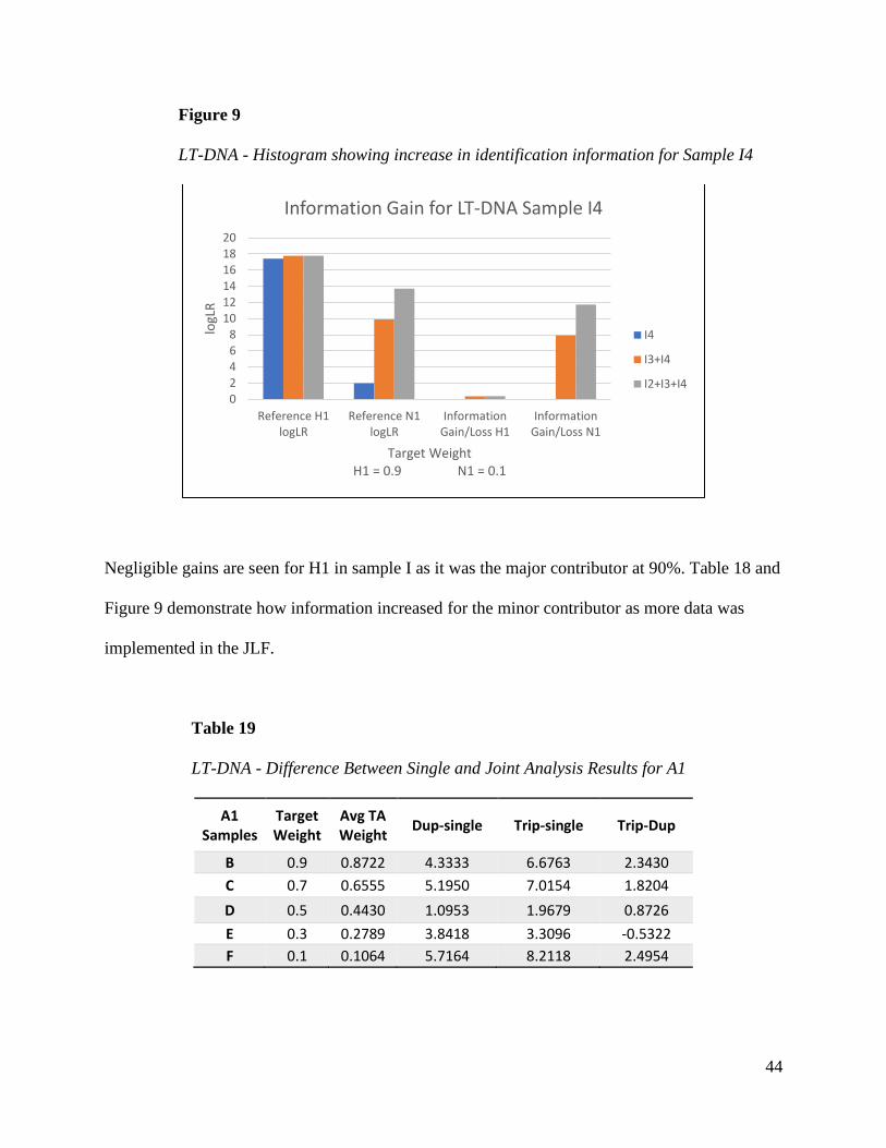
Table 19

LT-DNA - Difference Between Single and Joint Analysis Results for A1

A1 Samples

Target Weight

Avg TA Weight

Dup-single Trip-single Trip-Dup

B 0.9 0.8722 4.3333 6.6763 2.3430

C 0.7 0.6555 5.1950 7.0154 1.8204

D 0.5 0.4430 1.0953 1.9679 0.8726

E 0.3 0.2789 3.8418 3.3096 -0.5322

F 0.1 0.1064 5.7164 8.2118 2.4954

02468

101214161820

Reference H1logLR

Reference N1logLR

InformationGain/Loss H1

InformationGain/Loss N1

logL

R

Target WeightH1 = 0.9 N1 = 0.1

Information Gain for LT-DNA Sample I4

I4

I3+I4

I2+I3+I4

45

Table 20

LT-DNA - Difference Between Single and Joint Analysis Results for G1

G1 Samples

Target Weight

Avg TA Weight

Dup-single Trip-single Trip-Dup

B 0.1 0.1278 5.3227 17.1853 11.8626

C 0.3 0.3445 10.1584 11.8278 1.6694

D 0.5 0.5555 6.6943 6.2894 0.6687

E 0.7 0.7211 3.6723 2.7292 -0.9431

F 0.9 0.8942 0.0035 -0.0046 -0.0081

Tables 19 and 20 show the difference between single and joint analysis for references A1

and G1. Information gain is again greatest in the samples where the references have 10% mixture

weight. This increase continues from duplicate to triplicate analysis. A minor decrease in

identification information is seen for reference G1 when its weight is 90% between the triplicate

and single sample.

Sample C also shows an increase of information for A1 and G1 that is not expected. This

was due to differences in the target weight and the weights calculated by TrueAllele in the

individual analysis data for C4. TrueAllele determined that C4 had a ratio close to 50/50 in the

single analysis. Despite the TrueAllele average weight for sample C being close to the target

weight, the difference between single and joint analysis shows a gain consistent with mixture

weight combinations of 50/50 samples and unequal weighted samples. Figures 10 and 11 show

the histograms for A1 and G1.

46

Figure 10

LT-DNA - Histogram showing change in identification information for A1

Figure 11

LT-DNA - Histogram showing change in identification information for G1

-1

0

1

2

3

4

5

6

7

8

9

0.9 0.7 0.5 0.3 0.1

B C D E F

logL

R

Target WeightSample Group

Information Gain/Loss for Reference A1LT-DNA

Dup-single

Trip-single

Trip-Dup

-202468

101214161820

0.1 0.3 0.5 0.7 0.9

B C D E F

logL

R

Target WeightSample Group

Information Gain/Loss for Reference G1LT-DNA

Dup-single

Trip-single

Trip-Dup

47

Tables 21 and 22 show the gain in identification information using joint analysis for

references H1 and N1. Reference H1 showed the similar anomaly in sample L as was seen for

references A1 and G1 in sample C. Both samples were a 70/30 mixture weight. Though

unexpected, information gain was still the result. Reference N1 showed the expected trend as

seen in sample I where gain in information increased when low template minor contributor

samples were analyzed jointly with other samples. Figures 12 and 13 show the histograms for

references H1 and N1. Sample K showed the least amount of information gain as expected for a

50/50 mixture, but a small gain was still observed.

Table 21

LT-DNA - Difference Between Single and Joint Analysis Results for H1

H1 Samples

Target Weight

Avg TA Weight

Dup-single Trip-single Trip-Dup

I 0.9 0.8849 0.3675 0.3726 0.0051

J 0.7 0.6708 3.0218 7.1139 4.0921

K 0.5 0.5014 1.2561 0.6962 -0.5599

L 0.3 0.3183 14.9122 14.8888 -0.0234

M 0.1 0.1777 6.9408 7.9544 1.0136

Table 22

LT-DNA - Difference Between Single and Joint Analysis Results for N1

N1 Samples

Target Weight

Avg TA Weight

Dup-single Trip-single Trip-Dup

I 0.1 0.1151 7.8979 11.7279 3.8300

J 0.3 0.3292 5.1346 11.6317 6.4971

K 0.5 0.4987 2.297 1.4597 -0.8373

L 0.7 0.6818 3.4085 3.8735 0.4650

M 0.9 0.8223 0.9152 0.9154 0.0002

48

Figure 12

LT-DNA - Histogram showing change in identification information for H1

Figure 13

LT-DNA - Histogram showing change in identification information for N1

-2

0

2

4

6

8

10

12

14

16

0.9 0.7 0.5 0.3 0.1

I J K L M

logL

R

Target WeightSample Group

Information Gain/Loss for Reference H1LT-DNA

Dup-single

Trip-single

Trip-Dup

-2

0

2

4

6

8

10

12

14

0.1 0.3 0.5 0.7 0.9

I J K L M

logL

R

Target WeightSample Group

Information Gain/Loss for Reference N1LT-DNA

Dup-single

Trip-single

Trip-Dup

49

Complex Mixtures

This data set provided a close simulation to evidence data where mixture weight,

template concentration, and number of contributors are random making mixture analysis

difficult. The application of the JLF in this data set resulted in significant incremental gain in

information for the contributor with the lowest MW. Reversing the roles of major and minor

contributors was a consideration made when selecting these complex samples. The data

complemented each other well when analyzed jointly. The information gain for reference K01 as

the more minor contributor in sample 3.6 is shown in Table 23 and in Figure 14. Reference ASB

is the major contributor in this sample and the logLR remains relatively unchanged with each

analysis method.

Table 23

Difference Between Single and Joint Analysis Results for Complex Mixture 3.6

Sample Mixture Weight

(ASB/K01) Reference ASB

logLR Reference K01

logLR

Information Gain/Loss

ASB

Information Gain/Loss

K01

3.6 0.9006/0.0254 20.3219 3.3181

1.1 + 3.6 0.1349 + 0.8729/ 0.5015 + 0.0612

20.3211 13.5960 -0.0008 10.2779

1.1 + 3.6 + 4.2 0.4466 + 0.8616 + 0.0521/ 0.4656 + 0.0286 + 0.6233

20.3219 18.1666 0.0000 14.8485

50

Figure 14

Histogram showing change in identification information for Sample 3.6

Table 24

Difference Between Single and Joint Analysis Results for Complex Mixture 4.2

Sample Mixture Weight

ASB/K01) Reference ASB

logLR Reference K01

logLR

Information Gain/Loss

ASB

Information Gain/Loss

K01

4.2 0.1372/0.5404 0.7290 17.3530

1.1 + 4.2 0.4383 + 0.0846/ 0.2851 + 0.5493

16.6537 17.5757 15.9247 0.2227

3.6 + 4.2 0.9076 + 0.0538/ 0.0193 + 0.5782

20.3219 17.9900 19.5929 0.6370

1.1 + 3.6 + 4.2 0.4466 + 0.8616 + 0.0521/ 0.4656 + 0.0286 + 0.6233

20.3219 18.1666 19.5929 0.8136

-5.0000

0.0000

5.0000

10.0000

15.0000

20.0000

25.0000

ReferenceASB logLR

ReferenceK01 logLR

InformationGain/Loss ASB

InformationGain/Loss K01

log

LR

Mixture WeightASB = 0.88 K01 = 0.04

Information Gain/Loss for K01/ASB in Sample 3.6

3.6

1.1 + 3.6

1.1 + 3.6 + 4.2

51

Figure 15

Histogram showing change in identification information for Sample 4.2

Sample 4.2 reversed the roles for references ASB and K01. ASB was the minor

contributor and a significant information gain of 16 and 20 ban was obtained when sample 4.2

was analyzed jointly with samples 1.1 and 3.6 in duplicates and triplicate, respectively, as seen in

Table 24 and Figure 15. As the major contributor, reference K01 had large logLRs regardless of

analysis method but did have slight information gain unlike reference ASB when it was the

major contributor in sample 3.6.

Table 25

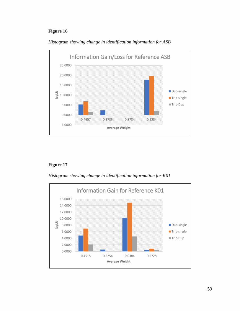
Change in Identification Information for Reference ASB

ASB Samples

Avg Weight

Dup-single Trip-single Trip-Dup

1.1 0.4657 5.3039 6.9026 1.5987

2.8 0.3785 2.3963

3.6 0.8784 -0.0008 0.0000 0.0008

4.2 0.1234 17.7588 19.5929 1.8341

0.0000

5.0000

10.0000

15.0000

20.0000

25.0000

ReferenceASB logLR

ReferenceK01 logLR

InformationGain/Loss ASB

InformationGain/Loss K01

logL

R

Mixture WeightASB = 0.12 K03 = 0.57

Information Gain for Reference ASB in Sample 4.2

4.2

1.1 + 4.2

3.6 + 4.2

1.1 + 3.6 + 4.2

52

Table 26

Change in Identification Information for Reference K01

K01 Samples

Avg Weight

Dup-single Trip-single Trip-Dup

1.1 0.4515 4.8367 6.9709 2.1342

2.8 0.6254 0.5662

3.6 0.0384 10.2779 14.8485 4.5706

4.2 0.5728 0.4298 0.8136 0.3837

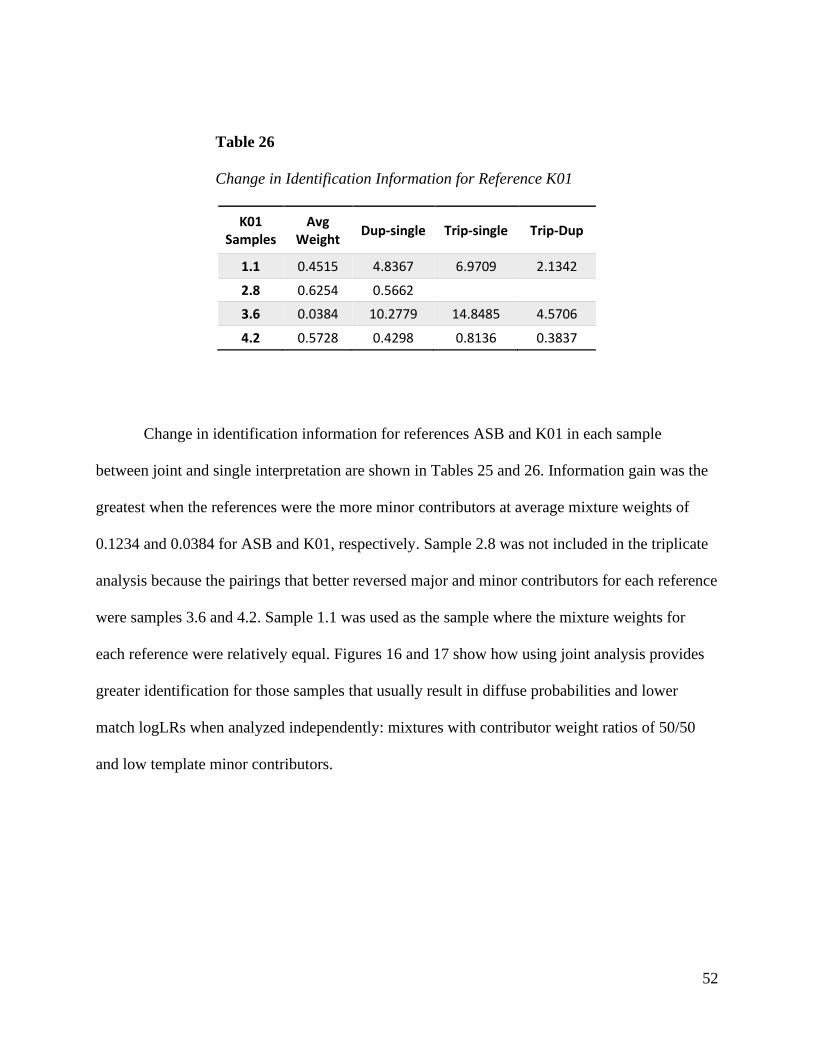
Change in identification information for references ASB and K01 in each sample

between joint and single interpretation are shown in Tables 25 and 26. Information gain was the

greatest when the references were the more minor contributors at average mixture weights of

0.1234 and 0.0384 for ASB and K01, respectively. Sample 2.8 was not included in the triplicate

analysis because the pairings that better reversed major and minor contributors for each reference

were samples 3.6 and 4.2. Sample 1.1 was used as the sample where the mixture weights for

each reference were relatively equal. Figures 16 and 17 show how using joint analysis provides

greater identification for those samples that usually result in diffuse probabilities and lower

match logLRs when analyzed independently: mixtures with contributor weight ratios of 50/50

and low template minor contributors.

53

Figure 16

Histogram showing change in identification information for ASB

Figure 17

Histogram showing change in identification information for K01

-5.0000

0.0000

5.0000

10.0000

15.0000

20.0000

25.0000

0.4657 0.3785 0.8784 0.1234

logL

R

Average Weight

Information Gain/Loss for Reference ASB

Dup-single

Trip-single

Trip-Dup

0.0000

2.0000

4.0000

6.0000

8.0000

10.0000

12.0000

14.0000

16.0000

0.4515 0.6254 0.0384 0.5728

logL

R

Average Weight

Information Gain for Reference K01

Dup-single

Trip-single

Trip-Dup

54

Conclusion

Higher match statistics were consistently obtained when samples were analyzed jointly

compared to the independent analysis of each sample. Mixture weight and template

concentration played a significant role in how much identification information was elicited from

the data when analyzed in duplicate and triplicate. Information gain was seen consistently in all

the samples but in greater amounts for samples with a 50/50 mixture weight and for contributors

whose weights were close to or lower than 10%. Overall, major contributors saw little to no

change in their match logLR values but in several cases a slight increase was observed.

These research results impact the field of forensic biology analysis because joint

likelihood functions can increase the probability distribution across all loci resulting in higher

match statistics. This would support using PG as the standard for complex mixture interpretation.

Another suggestion would be to modify DNA evidence collection and amplification procedures

for LT-DNA and mixture samples so that more data is available for PG software programs like

TrueAllele to analyze the data jointly using the JLF (Ballantyne et al., 2013). Certain limitations

can exist with using TrueAllele which include cost of purchasing the software and understanding

the mathematical and statistical concepts inherent with PG.

Future directions of this research would be to generate laboratory data and use TrueAllele

mixture interpretation to perform the analysis. Touch DNA samples can be collected using

multiple swabs to provide the independent sets of data needed for joint analysis. Different

substrates such as glass, plastic, wood, metal, etc. can be used to assess how much touch DNA is

retrieved from different surfaces and if probabilistic genotyping can preserve the identification

information using joint likelihood functions.

55

References

Ballantyne, J., Hanson, E. K., & Perlin, M. W. (2013). DNA mixture genotyping by probabilistic

computer interpretation of binomially-sampled laser captured cell populations:

Combining quantitative data for greater identification information. Science and Justice,

53(2), 103-114. https://doi.org/10.1016/j.scijus.2012.04.004

Bauer, D. W., Butt, N., Hornyak, J. M., & Perlin, M. W. (2020). Validating TrueAllele®

Interpretation of DNA Mixture Containing up to Ten Unknown Contributors. Journal of

Forensic Sciences, 65(2), 380-398. https://doi.org/10.1111/1556-4029.14204

Butler, J. M. (2005). Forensic DNA Typing: Biology, Technology, and Genetics of STR Markers

(2nd ed.) Academic Press.

Butler, J. M. (2010). Fundamentals of Forensic DNA Typing. Academic Press.

Butler, J. M. (2015). Advanced Topics in Forensic DNA Typing: Interpretation. Academic Press.

Gill, P., Gusmão, L., Haned, H., Mayr, W. R., Morling, N., Parson, W., Prieto, L., Prinz, M.,

Schneider, H., Schneider, P. M., & Weir, B. S. (2012). DNA commission of the

International Society of Forensic Genetics: Recommendations on the evaluation of STR

typing results that may include drop-out and/or drop-in using probabilistic methods.

Forensic Science International: Genetics, 6(6), 679-688.

https://doi.org/10.1016/j.fsigen.2012.06.002

Greenspoon, S. A., Schiermeier-Wood, L., & Jenkins, B. C. (2015). Establishing the Limits of

TrueAllele® Casework: A Validation Study. Journal of Forensic Sciences, 60(5), 1263-

1276. https://doi.org/10.1111/1556-4029.12810

Hornyak, J. M., Herbert, T., Allan, W. P., & Perlin, M. W. (2015, August 4). Baltimore Police

Department TrueAllele® Validation. Cybergenetics.

56

Kwong, K. (2017). The Algorithm Says You Did It: The Use of Black Box Algorithms to

Analyze Complex DNA Evidence. Harvard Journal of Law & Technology, 31(1), 275-

301. http://jolt.law.harvard.edu/assets/articlePDFs/v31/31HarvJLTech275.pdf

National Institute of Standards and Technology. (2014). NIST 1036 U.S. Population Dataset – 29

autosomal STR loci and 23 Y-STR loci. STRBase (SRD-130). Retrieved November 10,

2020, from https://strbase.nist.gov/NISTpop.htm

Perlin, M. W. (2013). When Good DNA Goes Bad. Journal of Forensic Research, S11(3).

http://dx.doi.org/10.4172/2157-7145.S11-003

Perlin, M. W. (2015). Inclusion probability for DNA mixtures is a subjective one-sided match

statistic unrelated to identification information. J Pathol Inform, 6(59).

DOI: 10.4103/2153-3539.168525

Perlin, M. W., Belrose, J. L., Duceman, B. W. (2013). New York State TrueAllele® Casework

Validation Study. Journal of Forensic Sciences, 58(6), 1458-1466.

https://doi.org/10.1111/1556-4029.12223

Perlin, M. W., Dormer, K., Hornyak, J. M., Schiermeier-Wood, L., & Greenspoon, S. (2014).

TrueAllele Casework on Virginia DNA Mixture Evidence: Computer and Manual

Interpretation in 72 Reported Criminal Cases. PLOS ONE, 9(3), Article e92837.

https://doi.org/10.1371/journal.pone.0092837

Perlin, M. W. & Galloway, J. (2012, May-June). Computer DNA Evidence Interpretation in the

Real IRA Massereene Terrorist Attack. Evidence Technology Magazine, 10(3), 20-23.

https://www.nxtbook.com/nxtbooks/evidencetechnology/20120506/index.php?startid=20

#/p/20

Perlin, M. W., Hornyak, J. M., Sugimoto, G., & Miller, K. W. P. (2015). TrueAllele® Genotype

57

Identification on DNA Mixtures Containing up to Five Unknown Contributors. Journal

of Forensic Sciences, 60(4), 857-868. https://doi.org/10.1111/1556-4029.12788

Perlin, M. W., Kadane, J. B., & Cotton, R. W. (2009). Match likelihood ratio for uncertain

genotypes. Law, Probability and Risk, 8(3), 289–302. https://doi.org/10.1093/lpr/mgp024

Perlin, M. W., Legler, M. M., Spencer, C.E., Smith, J. L., Allan, W. P., Belrose, J. L., &

Duceman, B. W. (2011). Validating TrueAllele® DNA Mixture Interpretation.

Journal of Forensic Sciences, 56(6), 1430-1447.

https://doi.org/10.1111/j.1556-4029.2011.01859.x

Perlin, M. W. & Sinelnikov, A. (2009). An Information Gap in DNA Evidence Interpretation.

PLoS One 4(12): e8327. https://doi.org/10.1371/journal.pone.0008327

Perlin, M. W. & Szabady, B. (2001). Linear Mixture Analysis: A Mathematical Approach

to Resolving Mixed DNA Samples. Journal of Forensic Sciences, 46(6), 1372-

1378. https://doi.org/10.1520/JFS15158J