Decoherence and de nite outcomes - arXiv · Decoherence and de nite outcomes Klaus Colanero ... and...

Decoherence and definite outcomes

Klaus Colanero

Universita degli Studi di Firenze

arX

iv:1

208.

0904

v1 [

quan

t-ph

] 4

Aug

201

2

This work by Klaus Colanero is licensed under a Creative Commons byAttribution license: http://creativecommons.org/licenses/by/3.0/

2

http://creativecommons.org/licenses/by/3.0/

Contents

1 Introduction 7

2 The problem 102.1 Superposition states and measurement outcomes . . . . . . . . 11

2.1.1 Inconsistent epistemic probability interpretation . . . . 122.1.2 Non-diagonal terms and interference . . . . . . . . . . 14

2.2 Von Neumann measurement theory . . . . . . . . . . . . . . . 152.2.1 Standard Copenhagen position . . . . . . . . . . . . . 172.2.2 General decoherence proposal . . . . . . . . . . . . . . 19

2.3 Observation of macroscopic superpositions . . . . . . . . . . . 222.3.1 Double-slit type experiments . . . . . . . . . . . . . . . 232.3.2 Quantum state control experiments . . . . . . . . . . . 262.3.3 Macroscopic superposition realization . . . . . . . . . . 27

2.4 Summary of main issues . . . . . . . . . . . . . . . . . . . . . 30

3 Definite outcomes in different interpretations 333.1 Theory extending solutions: adding new principles . . . . . . . 35

3.1.1 Copenhagen interpretation . . . . . . . . . . . . . . . . 353.1.2 Bohmian mechanics and hidden variables . . . . . . . . 373.1.3 Objective collapse theories . . . . . . . . . . . . . . . . 40

3.2 Interpretative solutions: understanding what we see . . . . . . 443.2.1 Relative state interpretation . . . . . . . . . . . . . . . 44

4 The decoherence approach 504.1 Decay of interference terms . . . . . . . . . . . . . . . . . . . . 51

4.1.1 Decoherence mechanism . . . . . . . . . . . . . . . . . 524.1.2 Decoherence time . . . . . . . . . . . . . . . . . . . . . 584.1.3 The essence of decoherence . . . . . . . . . . . . . . . . 65

4.2 Robust pointer states . . . . . . . . . . . . . . . . . . . . . . . 674.3 Implications for different interpretations . . . . . . . . . . . . 71

4.3.1 Environment assisted invariance and the Born rule . . 74

3

CONTENTS

4.4 Limitations of the decoherence programme . . . . . . . . . . . 774.4.1 Common criticism . . . . . . . . . . . . . . . . . . . . 784.4.2 The problem of the state vector reduction remains . . . 79

5 Alternative approaches 835.1 Environment induced collapse . . . . . . . . . . . . . . . . . . 835.2 Impossibility theorems . . . . . . . . . . . . . . . . . . . . . . 875.3 Gravity induced collapse . . . . . . . . . . . . . . . . . . . . . 89

6 Conclusion 94

4

Acknowledgements

I would like to thank my supervisors, Professor Roberto Casalbuoni and Pro-fessor Elena Castellani, for their helpful suggestions and constructive criti-cism.

I would like to acknowledge insightful and clarifying discussions with Dr.Max Schlosshauer, Prof. Claus Kiefer and Prof. Osvaldo Pessoa.

Credit is also due to the teachers of the various Logic courses who, withtheir competence and teaching skills, allowed me to overcome my initial im-pression of having landed in the wrong place. I now have a stronger founda-tion and better tools to study Philosophy of Science.

Special thanks go to my classmates who benevolently welcomed this mucholder lad among their peers.

I thank my housemates who gracefully tolerated my studying style pecu-liarities and occasionally shared some philosophical discussion on the chiefsystems of the world.

Finally, I feel obliged to thank my parents and my sisters who trusted Iwas still a sane person when undertaking these further studies well beyondmy years of youth.

5

“The continuing dispute about quantum measurement theory...is between peo-ple who view with different degrees of concern or complacency the followingfact: so long as the wave packet reduction is an essential component, andso long as we do not know exactly when and how it takes over from theSchrodinger equation, we do not have an exact and unambiguous formula-tion of our most fundamental physical theory.”

J.S. Bell

6

Chapter 1

Introduction

In the last few years the general notion of decoherence in quantum mechanicshas become increasingly common among physicists, philosophers of physicsand quantum information scientists. And rightly so, because it representsboth a further application of the predictive and explicative power of quan-tum theory, and an attempt to break the stalemate situation with respect tothe interpretation of quantum mechanics. Powerful as it might be, however,the decoherence programme has not solved the measurement problem yet.Specifically, and contrary to some claims, it has not solved the definite out-comes problem, better known as the problem of the wave function collapse.Due to the wide scope of the decoherence programme, which could be sum-marized as the attempt to recover the classical phenomena from quantumphysics, the problem of definite outcomes happens to be often confused withother, loosely related, issues. Such a confusion is the main motivation of thisstudy.

This thesis has three aims:

• to clarify in detail the relation between the decoherence mechanism andthe problem of definite outcomes,

• to dispel common misconceptions about the measurement problem inquantum mechanics, and

• to present some recent alternative approaches in the quest for a satis-factory solution of the definite outcomes problem.

Since the last decade, it has become quite common, especially amongphysicists, to think that the successes of the decoherence programme in ex-plaining the emergence of classical phenomena have solved the measurementproblem. Such an idea is unfortunately incorrect because, while the deco-herence mechanism accounts very well for the disappearing of interference

7

1. Introduction

in macroscopic systems and provides an enlightening understanding for theappearance of preferred robust pointer states, it does not offer, by itself, anexplanation for the apparent collapse of the state vector.

At a time when the decoherence programme is becoming well defined bothin its scope and in its physical and mathematical foundations, it seems neces-sary to identify in detail the place of definite outcomes within the decoherenceframework. This appears all the more relevant considering the promising andfascinating developments in experimental techniques for macroscopic quan-tum state control on the one hand, and in quantum information and compu-tation on the other.

Also, it is still difficult to overstate the importance of reducing misconcep-tions about the measurement problem in quantum mechanics. After abouteighty years since the formulation of the Schrodinger equation and the un-precedented success of quantum theory, it is quite peculiar that the problemof definite outcomes is still considered by most either a metatheoretical is-sue to be dealt with by means of a consistent interpretation, or a problemalready solved for all practical purposes by the decoherence programme. Asa matter of fact, not all practical issues are addressed by the decoherenceprogramme. At the same time it is legitimate and reasonable to try and lookfor solutions to the problem within physics itself, either through an even finergrained analysis of system–apparatus–environment dynamics, or through theintroduction of new physical laws whose consequences can be subjected toexperimental test.

With regard to the physics based approach to the problem, theoreticalconstraints to its viability are examined and recent proposals for feasibleexperimental tests are introduced.

What is not in the scope of this work is a complete review of the resultsand successes of the decoherence programme in explaining the emergence ofclassical phenomena from quantum dynamics. Instead, as the title suggests,the focus will be specifically on the relation between decoherence and defi-nite outcomes. In the same spirit, the different interpretations of quantummechanics are not presented in a comprehensive manner, but they are ana-lyzed from the specific point of view of the definite outcomes problem andwith respect to the theoretical and experimental results of the decoherenceprogramme.

In pursuing the aims listed above, philosophical assumptions and im-plications of each approach are explicitly analyzed in order to have a cleardistinction between physical, logical and metaphysical issues involved. Weak-nesses and merits of the various theoretical and interpretive approaches arehighlighted.

This thesis is organized as follows. In Chapter 2 the definite outcomes

8

problem is defined and analyzed. Recent experiments on superposition statesof macroscopic systems are examined and their implications for the standardinterpretation pointed out. The basic ideas of the decoherence formalism arealso introduced, in order to provide a clear foundation for the subsequentconsiderations.

In Chapter 3 the most commonly adopted interpretations are reviewedwith particular attention to the issue of definite outcomes and the applicationof the decoherence programme. In order to underline the different approacheswith respect to state vector reduction, the interpretations are grouped intheory extending solutions and interpretive solutions.

Chapter 4 is devoted to the theory of decoherence. Attention is put onidentifying the essential and general aspects within the great formal diver-sity in the application of the theory to different systems. The analysis isagain focused on clarifying connections and implications for the definite out-comes problem. Misconceptions with regard to merits and limitations of thedecoherence programme are addressed.

Environment-induced and gravity-induced collapse proposals are discussedin Chapter 5. The impossibility of a “for all practical purposes” solution ofthe definite outcomes problem, based on an environment-induced collapse, isdiscussed.

9

Chapter 2

The problem

From a very general and interpretation agnostic point of view, the problemof definite outcomes can be described as follows. According to quantumtheory a physical system can be in any of the infinitely many possible statesrepresented by a vector in the Hilbert space associated to the system. As amatter of fact, any time the system is observed it is found in one of only afew possible states: the ones corresponding to a definite value of the physicalquantity which is effectively being measured through the observation. If, forexample, the state of a spin 1/2 system is α |↑〉+β |↓〉, an observer measuringthe value of the spin will either find the system in the up state, |↑〉, or inthe down state, |↓〉. On the contrary, even though it is not clear what wouldconstitute the observation of states such as α |↑〉+ β |↓〉, it appears that thesystem, upon observation, is never found in this kind of state.

Given such a state of affairs, one has to work out whether the explanationof the definite outcomes lies in (1) the addition of one or more postulates tothe basic building blocks given by the unitary and deterministic Schrodingerevolution, in (2) a suitable interpretation of the relation between the mathe-matical ingredients of the theory and what happens in the world, or even (3)directly within the unitary evolution of the wave function of the universe.

Obviously, a suitable interpretation is always necessary for any physicaltheory to be able to connect the formalism to the world, but such an interpre-tation might also include propositions which are later found to be redundantbecause they can be derived by the mathematical formalism and by the otherinterpretative postulates. In this regard, as it will become clear in the fol-lowing sections, a typical example is Bohr’s postulate that the measurementapparatus is governed by classical physics and not by quantum mechanics.

In the following section, the above mentioned issues will be presented ina formal and detailed manner. Moreover, the basic ideas at the heart of twodifferent approaches to the measurement problem will be presented.

10

2.1. Superposition states and measurement outcomes

2.1 Superposition states and measurement out-

comes

While in classical mechanics the state of a system is represented by a pairof conjugate variables {Q,P}, e.g. position and momentum of an object, inquantum mechanics it is represented by a vector, |ψ〉, in the Hilbert spaceassociated to the system. The vector |ψ〉 can be written as a superpositionof a set of vectors which forms a complete basis for that Hilbert space. Theeigenstates of a Hermitian operator constitute such a complete set and thuswe can for example write:

|ψ〉 =∑k

αk |Ek〉 =

∫ψ(x) |x〉 dx, (2.1)

where |Ek〉 is the kth eigenvector of the total energy operator, i.e. the Hamil-tonian operator of the system, and |x〉 is the eigenvector of the position op-erator corresponding to position x. The coefficients αk and ψ(x)dx containthe information about the relative weight and phase of each basis vector. InEq.(2.1) the state vector |ψ〉 has been expressed in two different basis in orderto show that it can analogously be expressed in terms of a set of eigenvectorsof any Hermitian operator.

An arbitrary state |ψ〉 will always correspond to a superposition in somevector basis. If the system is, for example, in an eigenstate |Ei〉 of theHamiltonian, H, in general it will not be in an eigenstate of the momen-tum operator, p, but it will be in a superposition of momentum eigenstates,∫〈p|Ei〉 |p〉 dp.

As it has been mentioned, it is necessary that the mathematical formalismbe complemented with an interpretation, which specifies how to relate statevectors and the operations on them with the actual properties of the physicalsystem of interest. As a basic interpretative prescription it seems natural toconnect the eigenstates of a self-adjoint operator to a well defined propertyof the associated physical system. That is, more explicitly, if the state ofthe system is described by the eigenstate |p〉 of the momentum operator,then we expect it to possess a well defined value of the momentum p. Or,in other words, that the value p of the physical quantity momentum is anobjective property of the system. Such a prescription corresponds to the socalled eigenstate-eigenvalue link, or e-e-link, and it appears consistent withexperimental observations.

The first non-trivial issue, and a main aspect of the definite outcomesproblem, is that a priori it is not clear what physical properties should beassociated to a system described by a generic superposition. For example, it

11

2. The problem

is also not clear a priori what should be the meaning of measuring the energyof a system which is not in an eigenstate of the Hamiltonian operator, suchas∑

k αk |Ek〉.In order to build a clear picture of the problem it is helpful to consider

one of the simplest, yet powerfully explicative, quantum mechanical systems:a spin 1/2 system. The two eigenstates of the Sz operator, |+〉z and |−〉z,constitute a complete set of basis vectors for the two-dimensional Hilbertspace associated to the system.

If the system, say a single electron [1], is prepared in such a way that itis in one of the eigenstates of Sz, then it is more than reasonable to expectthat a Stern-Gerlach apparatus [2], set up in the z-direction, will providethe correct outcome for the eigenvalue of Sz, that is, the one correspondingto the actual state of the electron. But what if the state of the electron isα |+〉z + β |−〉z? What should we expect to see on the screen which recordsthe electron position after passing through the Stern-Gerlach apparatus? Atthis stage, without additional interpretative prescriptions, the answer is notobvious. And this is the first issue at the heart of the measurement problemin quantum mechanics.

2.1.1 Inconsistent epistemic probability interpretation

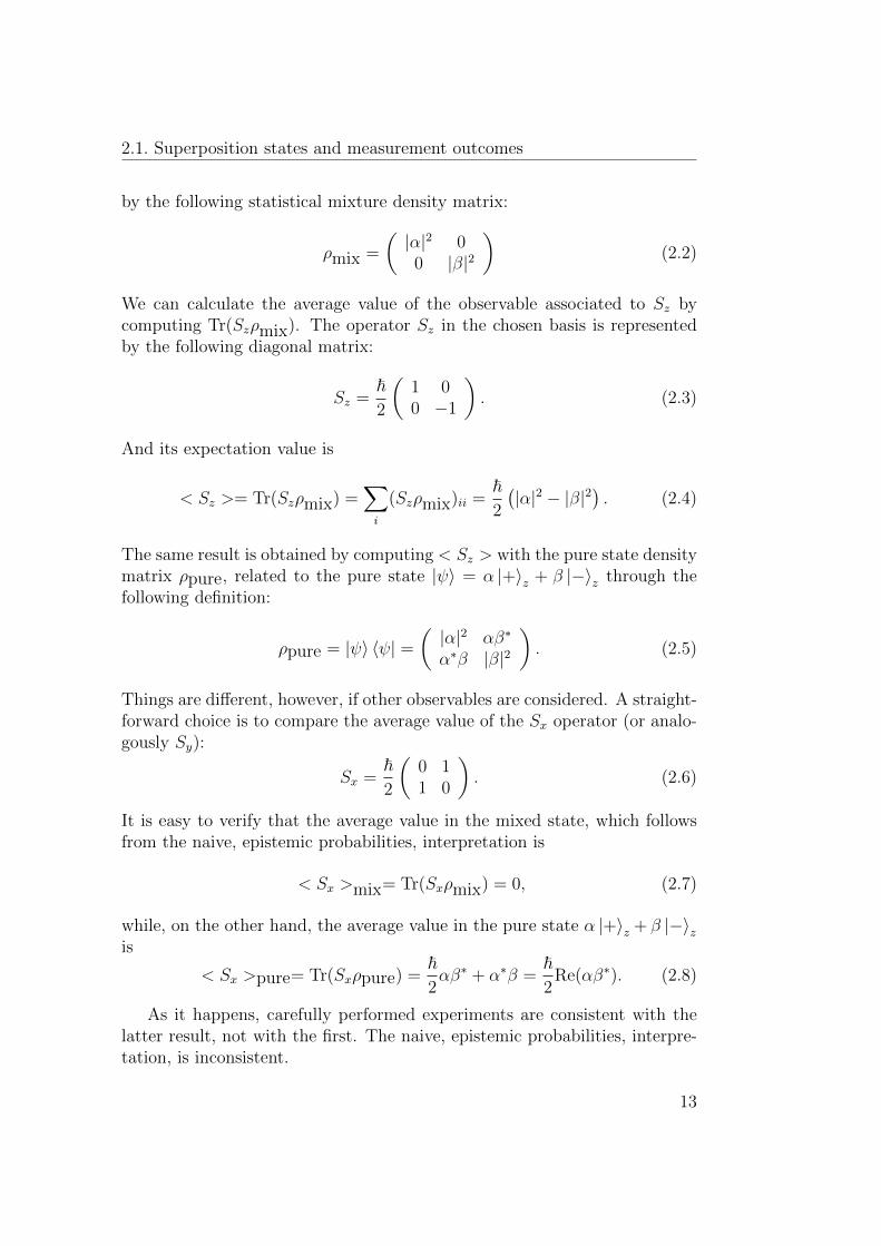
As a matter of fact, performing the above mentioned experiment with elec-trons in a superposition state, one sometimes observes a spot on the positioncorresponding to |+〉z, other times a spot on the position corresponding to|−〉z. Remarkably, it also happens that the relative frequencies of hits on theupper and lower spots converge to |α|2 and |β|2 respectively. This observa-tion immediately suggests a straightforward but inconsistent interpretationof superpositions: states for which the value of the observable of interestis not known, but only the probabilities of occurrence are known. Such anepistemic probability interpretation is inconsistent, because in general it doesnot produce correct predictions for the average values of observables. Thisbecomes particularly clear through the formalism of density matrices, whichallows to deal with pure states as well as actual statistical mixtures of statesin the same framework. In such a framework the state of a system is describedby a density matrix ρ which, analogously to the state vector, contains all theinformation about the system. The average value of any observable A resultsfrom the trace operation on the matrix Aρ.

According to the straightforward, naive, interpretation of superpositionstates, there is a |α|2 probability that the system is in the spin-up state and a|β|2 probability that it is in the spin-down state. Such a situation is described

12

2.1. Superposition states and measurement outcomes

by the following statistical mixture density matrix:

ρmix =

(|α|2 0

0 |β|2)

(2.2)

We can calculate the average value of the observable associated to Sz bycomputing Tr(Szρmix). The operator Sz in the chosen basis is representedby the following diagonal matrix:

Sz =~2

(1 00 −1

). (2.3)

And its expectation value is

< Sz >= Tr(Szρmix) =∑i

(Szρmix)ii =~2

(|α|2 − |β|2

). (2.4)

The same result is obtained by computing < Sz > with the pure state densitymatrix ρpure, related to the pure state |ψ〉 = α |+〉z + β |−〉z through thefollowing definition:

ρpure = |ψ〉〈ψ| =(|α|2 αβ∗

α∗β |β|2). (2.5)

Things are different, however, if other observables are considered. A straight-forward choice is to compare the average value of the Sx operator (or analo-gously Sy):

Sx =~2

(0 11 0

). (2.6)

It is easy to verify that the average value in the mixed state, which followsfrom the naive, epistemic probabilities, interpretation is

< Sx >mix= Tr(Sxρmix) = 0, (2.7)

while, on the other hand, the average value in the pure state α |+〉z + β |−〉zis

< Sx >pure= Tr(Sxρpure) =~2αβ∗ + α∗β =

~2

Re(αβ∗). (2.8)

As it happens, carefully performed experiments are consistent with thelatter result, not with the first. The naive, epistemic probabilities, interpre-tation, is inconsistent.

13

2. The problem

2.1.2 Non-diagonal terms and interference

The above considerations, which are standard in any introductory coursein quantum mechanics, are presented here in order to stress from the verybeginning the central place and the non-trivial nature of the definite outcomesproblem. Namely, even if one simply accepts that superposition states do notbelong to the world of observations, the relation between state vectors andthe actual observed phenomena is a matter of careful interpretation.

Before proceeding to define and address the core issue of the definiteoutcomes problem, it is instructive to make one more remark about thespin 1/2 system considered above: the difference between the two < Sx >results originates from the presence of the non-diagonal terms in the purestate density matrix. Such terms, which in a Stern-Gerlach type experimentmanifest themselves in a relatively subtle way in the averages < Sx > and< Sy >, show their effect drammatically in interference experiments, such aswith the double slit setup.

In a double slit interference experiment the state of the system, a par-ticle emerging from a barrier with two openings, can be described by thestate vector |ψ〉 = c1 |ψ1(t)〉 + c2 |ψ2(t)〉, where |ψ1(t = 0)〉 and |ψ2(t = 0)〉represent the state of a particle well localized around the first and the secondslit respectively. As it is shown in quantum mechanics textbooks, the squaremodulus of the wave function ψ(x, t), which as in Eq.(2.1) is the coefficient ofthe position eigenvector |x〉, acquires a typical, modulated, pattern with sev-eral minima and maxima, instead of just the two peaks one would expect fromparticles passing through one or the other slit. Such a pattern is directly re-lated to the mixed terms, c1c

∗2 〈ψ2(t)|x〉〈x|ψ1(t)〉 and c∗1c2 〈ψ1(t)|x〉〈x|ψ2(t)〉,

which appear in the expression for |ψ(x, t)|2. These also correspond to thenon-diagonal terms in the density matrix.

The above considerations, regarding the non-diagonal, or interference,terms, though not evidently central to the discussion on the definite out-comes problem, constitute one of the main issues addressed by the decoher-ence programme. Also they are too often either considered the only measure-ment problem or mixed up with the issue of definite outcomes to produce aconfused picture of the measurement problem. It is thus crucial to have aclear understanding of this aspect of quantum mechanical states.

In the following section the general approach to the description of themeasurement process within the quantum mechanical framework is presented,along with the issues it raises.

14

2.2. Von Neumann measurement theory

2.2 Von Neumann measurement theory

The process of measuring the properties of a physical system is perhaps themost subtle phenomenon to be dealt with in physics, at least because ulti-mately it has to deal, one way or another, with the properties and features ofan observer. Even with such complex problems, however, it makes sense andis always fruitful to adopt an analytical approach which starts from undis-putable or extremely reasonable assumptions. Regardless of the peculiaritiesof the observer, (1) one such assumption is that the measurement processof a quantum system involves the interaction between the system and themeasurement apparatus. Moreover (2) the apparatus is supposed to be com-posed of smaller parts whose behaviour is described by the laws of quantummechanics, specifically the Schrodinger equation. Finally, (3) the quantumsystem to be observed interacts with the macroscopic apparatus through itsconstituent quantum parts.

The just mentioned “extremely reasonable” assumptions are at the ba-sis of the Von Neumann scheme for modelling the measurement process.According to this scheme there is a quantum system Q with an associatedHilbert space HQ and a Hamiltonian HQ, and there is a measurement appa-

ratus M designed to measure the value of an observable A of the system Q.The dynamics of the macroscopic apparatus M also depends, through theSchrodinger equation, on a quantum Hamiltonian HM , and its associatedHilbert space is denoted by HM . The measurement takes place when thetwo systems, Q and M , interact by means of an interaction Hamiltonian HI

which can be considered different from zero only for a finite and relativelyshort time interval, the measurement time. The total system, comprised ofQ and M , is described by a state vector |Ψ〉 belonging to the Hilbert spacegiven by the tensor product of the two spaces, HQ ⊗HM .

The apparatus features a pointer from which the outcomes can be readout. The state of the apparatus can be represented by a vector |Φ〉 =∑

X,~y cX,~y |X, ~y〉M , where X is the eigenvalue of the pointer position oper-ator and ~y are the eigenvalues related to the other observables necessary tocompletely describe the state of the apparatus.

As a first and basic requirement, the apparatus should be able to re-veal the e-e-link, that is: for each distinct eigenstate of the operator A, thepointer will be in a distinct eigenstate of the position operator X. Beforethe measurement, system M is supposed to be in a “ready” state |X0〉M =∑

~y cX0,~y |X0, ~y〉M . Consequentely, if the state of Q is |a1〉Q, the total systemstate vector before the measurement is |Ψ〉in = |a1〉Q |X0〉M . After the mea-surement it should be |Ψ〉fin = |a1〉Q |X1〉M . In other words it is necessary

15

2. The problem

that the interaction Hamiltonian HI produces the following transition:

|ak〉Q |X0〉M =⇒ |ak〉Q |Xk〉M , (2.9)

where |Xk〉M represents a specific eigenstate of X which can be univocallyassociated to |ak〉Q. This is possible if the interaction Hamiltonian is of thefollowing type:

HI = g(t)P A, (2.10)

where A is the operator associated to the observable to be measured, P isthe adjunct operator of X, and g(t) is a real-valued function defined as

g(t) =

{g t0 < t < t0 + τ0 otherwise

(2.11)

During the measurement the state evolution is governed by the total Hamil-tonian, H = HQ +HM +HI , through the unitary evolution operator U(t) =exp− i

~Ht. If, however, the interaction is chosen strong enough to dominate,for short measurement times τ , the time evolution, then the effect of themeasurement interaction can be calculated, with good approximation, byneglecting the contribution of HQ +HM :

|Ψ(t0)〉 = |ak〉Q |X0〉M =⇒ |Ψ(t0 + τ)〉 = e−i~HIτ |Ψ(t0)〉 . (2.12)

Noting that for conjugate operators, like X and P , holds that

e−i~ P a |X〉 = |X + a〉 (2.13)

and applying the operator exp− i~gP Aτ first to |ak〉, then the final state

e−i~HIτ |Ψ(t0)〉 can be calculated as

e−i~gP Aτ |ak〉Q |X0〉M = |ak〉Q e

− i~gP akτ |X0〉M = |ak〉Q |X0 + akgτ〉M . (2.14)

The pointer has moved from X0 to Xk = X0 + akgτThe above derivation shows that a measurement apparatus can be de-

signed in such a way that, for each measured system eigenstate |ak〉, themeasurement process brings the pointer from the “ready” state |X0〉M toa distinct pointer position eigenstate |X0 + akgτ〉M . It is possible to con-

ventionally associate the eigenvalue ak of the operator A to this pointereigenstate. The apparatus is thus consistent with the e-e-link requirement.

Having addressed the interaction mechanism between system and appa-ratus, it is now possible to derive the final state of the apparatus after themeasurement on a generic state of the system Q, |ψ〉Q =

∑k ck |ak〉. Thanks

16


to the linearity of the time evolution operator U(t), it is straightforward tofind

|ψ〉Q |X0〉M =⇒∑k

e−i~gP Aτck |ak〉Q |X0〉M =

∑k

ck |ak〉Q |X0 + akgτ〉M .

(2.15)The apparatus is predicted to evolve from the measurement ready position toa superposition of pointer eigenstates! The superposition of the initial stateof system Q propagates to the macroscopic apparatus M through entangling,caused by the measurement interaction itself.

As a matter of fact, however, situations in which the pointer of a macro-scopic apparatus appears in a superposition state seem never to occur. Onthe contrary, definite pointer positions are always observed. This, cuttingthe frills, is the central issue about the definite outcomes problem.

2.2.1 Standard Copenhagen position

Highlighting the two main results presented so far, the definite outcomesproblem can be stated in more detail as follows:

• computation of statistical average values of observables show that su-perposition states are indeed different from classically not well definedstates, such as statistical mixtures, but

• such states, predicted to occur in macroscopic as well as microscopicsystems, are never directly observed in single measurements.

Before proceeding further, it is necessary to take into account anotherindirectly relevant phenomenon: the apparent lack of interference in experi-ments with macroscopic systems. In the previous section it has been statedthat carefully performed experiments agree with the calculations based on apure state density matrix, e.g. the result of Eq.(2.8). Experiments on sys-tems comprised of more than a few tens of atoms, however, provide a morepuzzling picture of the physical phenomena. Contrary to what is consistentlyfound for photons and electrons, statistical average values of observables turnout to agree with the predictions of a statistical mixture of definite states,like for example in Eq.(2.7). Likewise, interference experiments with systemslarger than a few atoms do not show interference patterns.

The so called Copenhagen interpretation of quantum mechanics is the firstsuccessful attempt at building a consistent framework to relate the results ofquantum theory to the experiments’ outcomes. Here by successful attemptit is meant consistent within the experimental accuracy reached at the time

17

2. The problem

the interpretation was proposed. The Copenhagen interpretation can besummarized in the following statements:

(i) The state vector |ψ〉 contains all the information about the system.

(ii) The time evolution of the vector |ψ〉 is governed by the Schrodingerequation.

(iii) An observer can access the system only through a macroscopic appara-tus which is subject to the laws of classical physics.

(iv) The measurement of the observable A changes the state of the systemfrom |ψ〉 to |ak〉, one of the eigenstates of A, breaking the unitaryevolution of the Schrodinger equation.

(v) The probability that the measurement process brings the system in thestate |ak〉 is given by |ck|2, the square modulus of the kth coefficient inthe expansion |ψ〉 =

∑i ci |ai〉.

Notice that statement (v) implies that, when the system is in an eigenstateof an observable A, it will be found in that state with probability 1. Asa consequence the corresponding eigenvalue is an objective property of thesystem.

The lack of interference for macroscopic objects and the problem of defi-nite outcomes are addressed by means of statements (iii) and (iv). Postulate(iii) tells why quantum effects are not observed macroscopically, and pos-tulate (iv) why specific, one-valued, outcomes are observed instead of thepredictions of Von Neumann measurement scheme. In other words, it is pos-tulated that the world is governed by different laws: quantum mechanics forthe microscopic world, and classical physics for the macroscopic, directly ac-cessible, world. Moreover, even though the microscopic system can actuallybe in a superposition state, in its interaction with a macroscopic apparatus,perhaps the observer herself, it will necessarily “collapse” to an eigenstatecorresponding to the observed physical quantity. The boundary betweenmicroscopic and macroscopic regime is not specified.

In the next chapter the Copenhagen interpretation will be analyzed inmore detail, but it can be safely said that, as puzzling and vague as it mayseem, it is not in contradiction with the experimental observations performedat the time it was proposed.

The first question that naturally comes to mind is whether statement (iii)correctly describes the physical state of affairs about macroscopic systems, orwhether it is an approximation of the actual quantum dynamics of complex,many particle systems. Equivalently, from a more formal point of view,

18


it is meaningful to ask whether statement (iii) is necessary for a completeinterpretation of quantum theory, or it can actually be derived through thecareful application of the other four statements to the study of macroscopicsystems.

The above questions have been addressed theoretically starting from the1970’s [3, 4] and experimentally only after the 1990’s [5, 6] due to the technicaldifficulties involved. The basic idea at the heart of the theoretical approach isthat the closed system idealization, usually employed in modelling the systemunder study, is often unsuitable. The reason is that, in the general case, theinteractions with particles in the environment, such as photons, electrons oratoms, and even the interaction with the internal degrees of freedom, greatlyaffect the dynamics of the system and thus cannot be neglected. The wideclaim, that the whole decoherence programme is committed to prove, is thatthe interaction of a system with a large number of particles, whose dynamicaldetails are not completely controlled by the observer, modifies the system’sbehaviour in such a way that it agrees with the laws of classical physics.Such a general aim is often described as the explanation for the emergenceof classicality from the quantum world.

As already mentioned, however, a complete investigation of the decoher-ence programme is not in the scope of the present work. On the contrary, inorder to clarify the connections between decoherence and definite outcomes,it can be more fruitful to focus on the relevant aspects. One of them isthe explanation of the lack of interference in macroscopic objects. The rel-evance of such issue to the definite outcomes problem lies in the fact that,if macroscopic superpositions are allowed, then the Von Neumann measure-ment scheme is valid at least within some, yet to be defined, domain.

2.2.2 General decoherence proposal

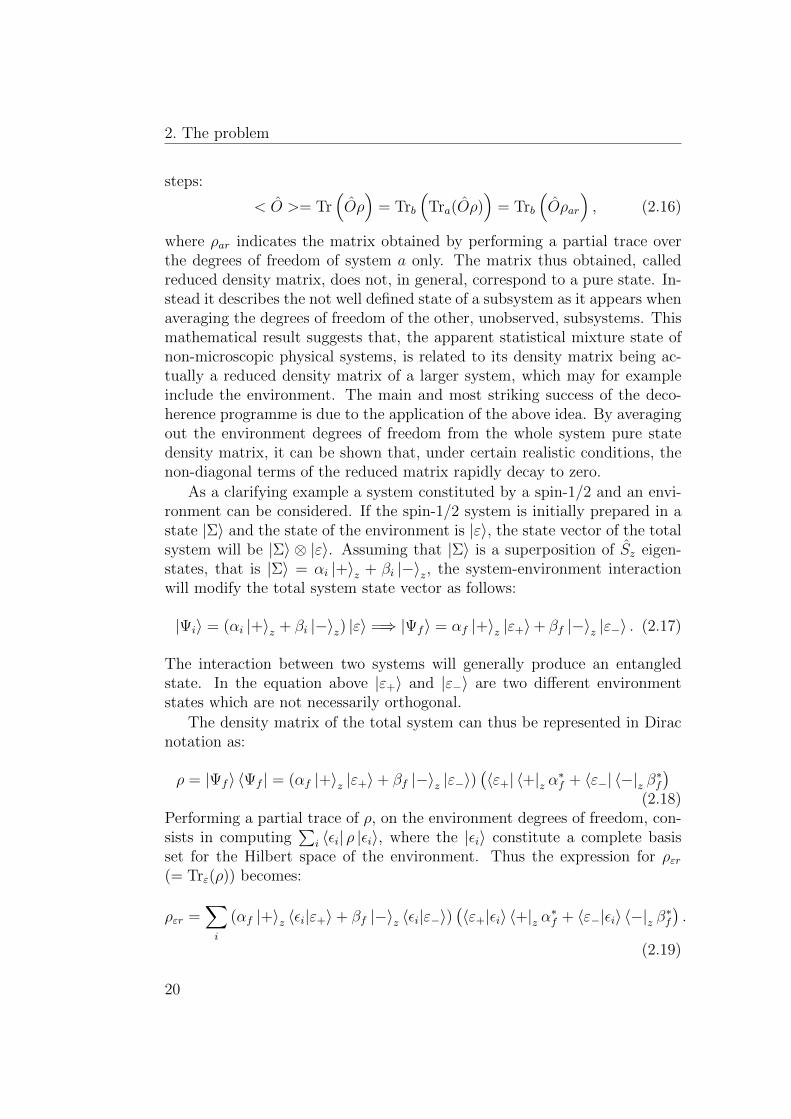
In Chapter 4 the decoherence approach will be presented in detail, but it isuseful to anticipate here its success in explaining the fast decay to zero of thenon-diagonal terms in the density matrix of the system under investigation.This result is arrived at by starting the study from the pure state densitymatrix of the “whole” physical system: system plus environment. As alreadymentioned, in Section 2.1.1 the average value of an observable O can becomputed by performing the trace of the matrix Oρ. In the case of a complexsystem, that is a system whose Hilbert space H is the tensor product ofseveral subsystems Hilbert spaces, e.g. H = Ha ⊗Hb, if the observable Ois associated to subsystem b only, the trace operation can be performed in

19

2. The problem

steps:

< O >= Tr(Oρ)

= Trb

(Tra(Oρ)

)= Trb

(Oρar

), (2.16)

where ρar indicates the matrix obtained by performing a partial trace overthe degrees of freedom of system a only. The matrix thus obtained, calledreduced density matrix, does not, in general, correspond to a pure state. In-stead it describes the not well defined state of a subsystem as it appears whenaveraging the degrees of freedom of the other, unobserved, subsystems. Thismathematical result suggests that, the apparent statistical mixture state ofnon-microscopic physical systems, is related to its density matrix being ac-tually a reduced density matrix of a larger system, which may for exampleinclude the environment. The main and most striking success of the deco-herence programme is due to the application of the above idea. By averagingout the environment degrees of freedom from the whole system pure statedensity matrix, it can be shown that, under certain realistic conditions, thenon-diagonal terms of the reduced matrix rapidly decay to zero.

As a clarifying example a system constituted by a spin-1/2 and an envi-ronment can be considered. If the spin-1/2 system is initially prepared in astate |Σ〉 and the state of the environment is |ε〉, the state vector of the totalsystem will be |Σ〉 ⊗ |ε〉. Assuming that |Σ〉 is a superposition of Sz eigen-states, that is |Σ〉 = αi |+〉z + βi |−〉z, the system-environment interactionwill modify the total system state vector as follows:

|Ψi〉 = (αi |+〉z + βi |−〉z) |ε〉 =⇒ |Ψf〉 = αf |+〉z |ε+〉+ βf |−〉z |ε−〉 . (2.17)

The interaction between two systems will generally produce an entangledstate. In the equation above |ε+〉 and |ε−〉 are two different environmentstates which are not necessarily orthogonal.

The density matrix of the total system can thus be represented in Diracnotation as:

ρ = |Ψf〉〈Ψf | = (αf |+〉z |ε+〉+ βf |−〉z |ε−〉)(〈ε+| 〈+|z α

∗f + 〈ε−| 〈−|z β

∗f

)(2.18)

Performing a partial trace of ρ, on the environment degrees of freedom, con-sists in computing

∑i 〈εi| ρ |εi〉, where the |εi〉 constitute a complete basis

set for the Hilbert space of the environment. Thus the expression for ρεr(= Trε(ρ)) becomes:

ρεr =∑i

(αf |+〉z 〈εi|ε+〉+ βf |−〉z 〈εi|ε−〉)(〈ε+|εi〉〈+|z α

∗f + 〈ε−|εi〉〈−|z β

∗f

).

(2.19)

20


Expanding the diadic form and considering that∑

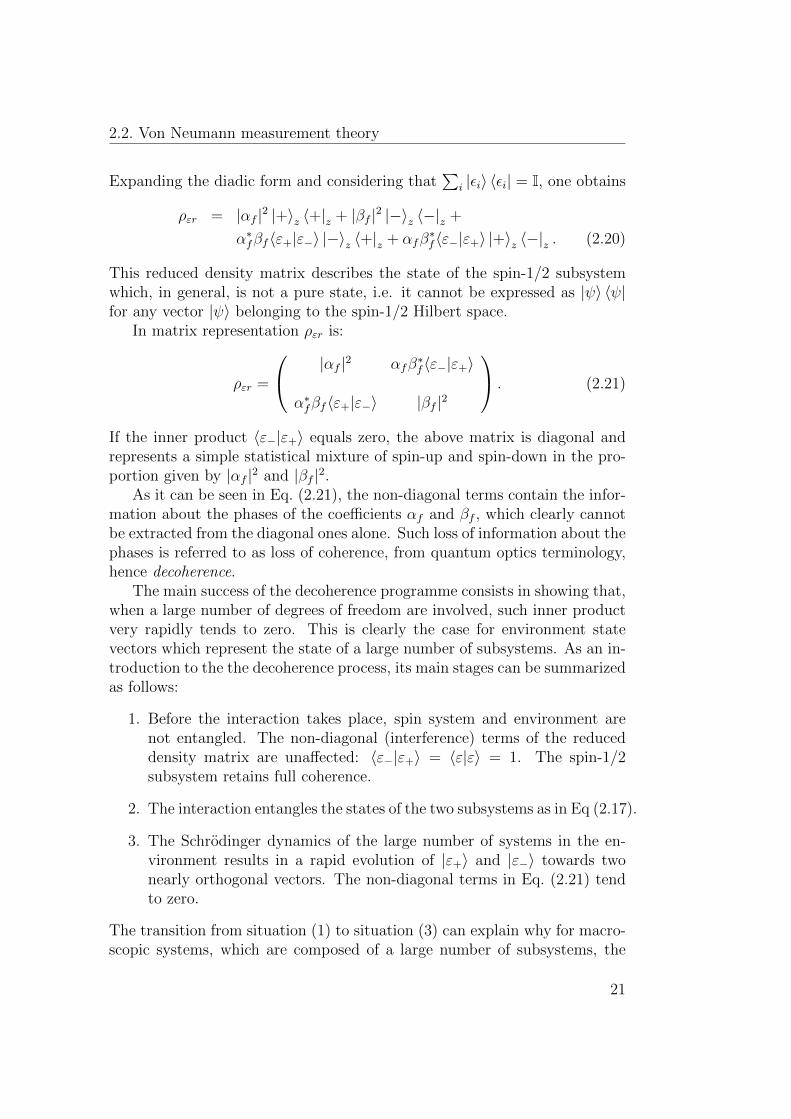
i |εi〉〈εi| = I, one obtains

ρεr = |αf |2 |+〉z 〈+|z + |βf |2 |−〉z 〈−|z +

α∗fβf〈ε+|ε−〉 |−〉z 〈+|z + αfβ∗f〈ε−|ε+〉 |+〉z 〈−|z . (2.20)

This reduced density matrix describes the state of the spin-1/2 subsystemwhich, in general, is not a pure state, i.e. it cannot be expressed as |ψ〉〈ψ|for any vector |ψ〉 belonging to the spin-1/2 Hilbert space.

In matrix representation ρεr is:

ρεr =

|αf |2 αfβ∗f〈ε−|ε+〉

α∗fβf〈ε+|ε−〉 |βf |2

. (2.21)

If the inner product 〈ε−|ε+〉 equals zero, the above matrix is diagonal andrepresents a simple statistical mixture of spin-up and spin-down in the pro-portion given by |αf |2 and |βf |2.

As it can be seen in Eq. (2.21), the non-diagonal terms contain the infor-mation about the phases of the coefficients αf and βf , which clearly cannotbe extracted from the diagonal ones alone. Such loss of information about thephases is referred to as loss of coherence, from quantum optics terminology,hence decoherence.

The main success of the decoherence programme consists in showing that,when a large number of degrees of freedom are involved, such inner productvery rapidly tends to zero. This is clearly the case for environment statevectors which represent the state of a large number of subsystems. As an in-troduction to the the decoherence process, its main stages can be summarizedas follows:

1. Before the interaction takes place, spin system and environment arenot entangled. The non-diagonal (interference) terms of the reduceddensity matrix are unaffected: 〈ε−|ε+〉 = 〈ε|ε〉 = 1. The spin-1/2subsystem retains full coherence.

2. The interaction entangles the states of the two subsystems as in Eq (2.17).

3. The Schrodinger dynamics of the large number of systems in the en-vironment results in a rapid evolution of |ε+〉 and |ε−〉 towards twonearly orthogonal vectors. The non-diagonal terms in Eq. (2.21) tendto zero.

The transition from situation (1) to situation (3) can explain why for macro-scopic systems, which are composed of a large number of subsystems, the

21

2. The problem

outcomes distribution does not reflect the underlying quantum statistics andappears instead as due to a classical statistical ensemble.

The same mechanism should apply to microscopic systems which are notwell screened from the interaction with surrounding particles and fields, andshould thus account for the fact that the outcomes of some experiments onmicroscopic systems correspond to a diagonal density matrix like Eq. (2.2),instead of Eq. (2.5).

In summary, the main result of the decoherence approach suggests thatpostulating classical physics laws for macroscopic systems (statement (iii)of the Copenhagen interpretation) is unnecessary and that there is no fun-damental difference between the laws for microscopic systems and those formacroscopic ones.

On the other hand it is evident that this achievement of the decoherenceprogramme does not address the issue of the state vector reduction (state-ment (iv)), and thus of the emergence of definite outcomes. This becomeseven clearer when considering the physical meaning of the formal operationof averaging over the unobserved degrees of freedom. In fact computation ofaverage values implies that one has assumed the Born rule (statement (v))which in turn implies the adoption of the projection postulate (statement(iv)) [7].

Nevertheless the decoherence mechanism, by predicting the occurrence ofmacroscopic superpositions, even though for very short times, maintains therelevance of the Von Neumann measurement scheme and opens up again thequestion of whether or not the unitary evolution breaks at some stage andof what would be such a stage.

2.3 Observation of macroscopic superpositions

The analysis carried out so far shows the main link between the standard in-terpretation, the decoherence approach and the problem of definite outcomes:the occurrence of macroscopic superpositions.

First, the standard interpretation postulates the collapse of the wavefunction of the system when observed. Secondly, the decoherence mechanismshows that the classical behaviour of a macroscopic apparatus can in principlebe derived from its quantum mechanical description. Finally, taking intoaccount these two points, if macroscopic systems can actually be observed insuperposition states, then only one of two conclusions follows: either (1) thereis no actual collapse of the state vector, or (2), if a wave function collapsedoes actually occur, then it cannot be attributed to the classical nature ofthe apparatus.

22

2.3. Observation of macroscopic superpositions

In recent years there has been an increasing number of experiments aimedat testing the quantum mechanical nature of macroscopic systems. To thisauthor’s knowledge none of them is explicitely designed for testing the col-lapse mechanism of the state vector. This can be justified by the fact thatdirect verification of the collapse of a single system wave function is beyondcurrent experimental techniques and indirect study of the collapse mecha-nism still very difficult [8, 9, 10]. Valuable insights about the problem ofdefinite outcomes can nevertheless be extracted from a careful analysis ofthe experiments. This is not always a straightforward exercise as it is alsonot always clear how to derive the implications of such experiments for otherfoundational issues. Aim of this section is to clarify what can be concludedwith regard to the definite outcomes from the analysis of some relevant ex-periments.

As mentioned, the experiments considered in this section are all de-signed for the general aim of verifying the predictions of quantum mechan-ics with respect to macroscopic systems and to improve the control on thesystem-environment interaction, and consequently on the system quantumbehaviour. For the purpose at hand such experiments can be divided in threegroups: double-slit type experiments, quantum state control, and macro-scopic superposition realization. Such a classification is certainly quite arbi-trary, but it can be helpful in order to clarify the different information thatcan be extracted from various experiments performed with a similar purpose.

2.3.1 Double-slit type experiments

Young’s double-slit experiment is by most considered the clearest example ofthe quantum behavior of an object. By many it is also considered the mostbeautiful experiment of nineteenth century [11].

In the traditional, Bohr inspired, complementarity view, double-slit in-terference experiments are designed to show the wave-particle duality of mi-croscopic systems. In the context of the present investigation, however, itis clear that such a position cannot be assumed a priori because it is basedon a specific interpretative solution to the definite outcomes problem. It isinstead meaningful to consider interference experiments just for what theyare: tests of the predictive power of quantum mechanics. According to theSchrodinger equation, the wave function of an isolated physical system, ini-tially prepared in an eigenstate of the momentum of its center of mass, in thepresence of a barrier with a double slit, will evolve to form a pattern of max-ima and minima, analogous to optical interference phenomena. Regardlessof whether wave function collapse occurs or not, if such interference patternis experimentally observed, then it is necessary to infer that the system does

23

2. The problem

not obey classical physics.Already in 1930 Estermann and Stern [12] successfully performed a diffrac-

tion experiment with He atoms and H2 molecules, thus showing that thepredictions of wave mechanics hold for composite, though microscopic, sys-tems too. However only in recent years, improved control on environmentperturbation and system preparation have allowed physicists to realisticallyattempt interference experiments with nearly macroscopic systems.

In 1999 Arndt et al. from the group of Anton Zeilinger [13] achieved oneof the first great leaps in size. They successfully observed the diffractionof C60, fullerene molecules, through a 100nm grating. The experimentallyobserved diffraction pattern is in excellent agreement with the theoretical one,obtained with a de Broglie wavelength, λ = h/Mv, computed considering Mas the total mass of the C60 molecule. The good quantitative agreement thusobtained, in the words of the authors themselves, is indication that eachC60 molecule interferes only with itself. In other words the effect is not dueto interference of individual smaller components, such as atoms, nuclei orelectrons.

A relevant aspect of this experiment is the analysis of possible decoher-ence effects. The successful realization of molecular diffraction implies thatphase coherence is not lost during the molecule flight from the source to thedetector. In the whole system–apparatus setup there are three main possiblecauses of decoherence: photon emission due to the molecule’s excited inter-nal degrees of freedom, photon absorption from the environment blackbodyradiation, and scattering of background molecules. The authors show that,in the case of this particular setup, all of them give a negligible contributionto decoherence.

A noteworthy detail in the article is the explanation of why photon emis-sion or absorption do not remarkably affect phase coherence. The authorscorrectly state that only photons with a wavelength shorter than the distancebetween neighboring slits can, with a single scattering, completely destroythe interference pattern. In fact, that could occasionally correspond to thedetection of the molecule through one particular slit. As Bohr would say,that would reveal the particle nature of the molecule and destroy interfer-ence. From a foundational and interpretative point of view, however, such anexplanation has to be handled with care. First because the “which-way” de-tection argument, though factually correct, supposes the collapse of the wavefunction; second and more importantly because the above argument is not di-rectly related to the decoherence mechanism mentioned in subsection 2.2.1,which explains the decay of the non-diagonal terms while maintaining theoverall superposition. To the authors’ credit it has to be said that the abovedistinctions are implicit in their article when they state that decoherence is

24


however also possible via multi-photon scattering, citing classical works ondecoherence [14, 15, 16].

With regard to the measurement problem the result by Arndt et al. isrelevant mainly for its demonstration of an almost macroscopic system in asuperposition state. It constitutes, in fact, a further evidence of the difficultyin justifying the standard ‘orthodox’ separation of the world in two kingdoms:a quantum–microscopic regime and a classical–macroscopic one, as impliedby statement (iii) in the previous section presentation. In order to have anidea of how macroscopic the system is, it is meaningful to notice that the deBroglie wavelength of the C60 molecules used in this experiment is 400 timessmaller than the diameter of the molecule.

In 2003 the same group [17] further improved on the size of the interferingmolecules by performing a similar experiment with fluorofullerene, C60F48,which is about twice as massive as C60. The latest and most impressivedemostration of this kind is however the one performed by Gerlich et al. in2011 [18]. The experiment shows interference of molecules composed of upto 430 atoms. In the authors’ own words the experiment proves the quantumwave nature and delocalization of compounds with a maximal size of up to60A, masses up to 6910AMU and de Broglie wavelengths down to 1pm.Such a wavelength is, in this case, 6000 times smaller than the size of theobject. This contrasts sharply with the common wisdom, according to whichinterference effects are always negligible when the size of the object is largerthan its de Broglie wavelength. The article also stresses that the interferenceobserved is due to the wavelength of the whole molecule as a single entity, incontrast to experiments with ‘macroscopic’ Bose-Einstein condensates, whereinterference is expected because the wavelength of the BEC is essentially thesame as the relatively large one of the single constituent atoms. With respectto the issue of macroscopic delocalization, the authors highlight the fact thatthe grating’s width corresponds, in a wave-particle complementarity view, toa path separation of almost two orders of magnitude larger than the size ofthe molecules.

What this latest experiment shows, as the earlier ones of its kind andmore strikingly, is that decoherence and definite outcomes are two distinctphenomena. In successful interference experiments decoherence is effectivelyprevented, while, evidently, the state of each single interfering object col-lapses in interaction with the detector. This point will be considered in moredetail in Section 2.4.

25

2. The problem

2.3.2 Quantum state control experiments

Achieving interference with larger and larger molecular compounds is cer-tainly a strong indication of the absence of a break up scale for quantumtheory, but molecules, even as large as proteins, are not what one imagineswhen thinking of macroscopic objects. Micromechanical systems consideredin recent years are much closer to the common notion of macroscopic system,particularly for their being visible at least with an optical microscope.

Probably the most ambitious programme to date for preparing a macro-scopic system in a superposition state is described in the paper by Marshallet al. [9] and further analyzed by Kleckner et al. [19]. The authors proposethe use of a special Michelson interferometer, where one of the cavity mirrorsis replaced by a tiny mirror attached to a micromechanical cantilever, as tocreate and observe superposition and entanglement of the photon-cantileversystem. The design of the experiment allows not only testing of various de-coherence mechanisms, but also of some wave function reduction models: theauthors in particular are interested in a gravity induced collapse proposal byPenrose [20] (see Section 5.3). Both papers show that, on the one hand, theexperiment is feasible in principle with current state-of-the-art technology,on the other hand, that an excellent control on the system-environment in-teraction has to be achieved in order to meet the conditions for unambiguousobservation of quantum phenomena. Chief among these conditions is theability to maintain the cantilever in its vibrational ground state when notinteracting. Because of their relatively large mass, in micromechanical oscil-lators the energy gap between different vibrational states is particularly small(corresponding to resonance frequencies of the order of tens of megahertz)and standard cryogenic methods for mechanical systems are not enough toachieve temperatures below the excitation energies of the oscillator [21].

Motivated by foundational issues as well as by technical application op-portunities, several groups have in recent years taken up the challenge ofrealizing quantum micromechanical systems. Directly relevant for the aboveproposed experiment are the works by O’Connel et al. [22] and by Teufel etal. [23]. In both experiments the micromechanical system is a cantilever andboth consist of about 1012 atoms, close to the 1014 atoms of the Bouwmeesterproposal [19]. Both micromechanical oscillators are coupled to a microwaveresonant circuit which acts as the measurement apparatus (whose signal isto be amplified). Remarkably, from the point of view of quantum computa-tion, in the 2010 experiment [22] the microwave resonant circuit is designedto realize a two-level system, and thus store a quantum bit of information.This is achieved by using a superconducting quantum interference device: aSQUID.

26


The two experiments differ substantially in the details of the actual im-plementation of the system-apparatus interaction and in the measurementreadout. They both succeed however in two common goals: cooling of theoscillator to its ground state and controlled single quantum excitation. Thesetup of O’Connel et al. allowed them to also observe the exchange of a quan-tized excitation between the oscillator and the SQUID, in agreement with thequantum mechanism of Rabi oscillations. As a further evidence of the quan-tum mechanical nature of the cantilever behavior, the authors successfullyplaced the system in a harmonic oscillator coherent state, as indicated by thegood agreement of the theory with the qubit response. On the other hand,the design by Teufel et al., thanks to the tunable coupling strength betweentheir mechanical resonator and a microwave cavity, can improve remarkablythe coherence time of the system state, extending it to over 100µs. This ismuch larger than typical decoherence times of SQUID based qubits and thusallows performing quantum operations on such a mechanical system.

In short, aside from the enormous scientific and technical achievementthese experiments constitute, their immediate relevance, with respect to themeasurement problem in general and the definite outcomes in particular,consists in demonstrating that naked-eye visible mechanical objects satisfyquantum physics. In fact the oscillator of Ref. [22] is about 50µm in two ofthe three dimensions and thus noticeable to the naked eye; the one of Ref [23]is about 20µm, slightly below the human eye capability.

2.3.3 Macroscopic superposition realization

As presented above, direct or indirect evidence of superposition states havebeen obtained for macromolecules and micromechanical oscillators. There isanother class of physical systems which is particularly suitable to test theoccurence of macroscopic superposition states: superconducting quantum in-terference devices, commonly referred to with the acronym of SQUIDs. Asuperconducting quantum interference device, in its most elementary form,consists of a superconducting loop cut by a small piece of insulating ma-terial and driven by an external magnetic flux. The junction between thesuperconductor and the insulator is called a Josephson junction and it isnarrow enough to allow Cooper pairs tunneling thus keeping the whole loopsuperconducting. Typical values of the supercurrent in a SQUID are in themicroampere range, corresponding to the collective motion of millions ofCooper pairs. The Josephson junction generates a potential energy term inthe Hamiltonian that describes the supercurrent and thus makes it possibleto design non trivial configurations such as, for example, with a double wellpotential.

27

2. The problem

Experimentally the basic idea is to prepare and observe the supercur-rent flowing in the ring in a superposition of clockwise and anticlockwisestates. Among the first breakthroughs in this regard, it is worth mentioningtwo indipendent experiments reported in 2000: one by Friedman et al. [24]and one by van der Wal et al. [25]. As was the case for the micromechan-ical oscillators, besides several differences in the implementation, the twoexperiments share all the main features: a radio frequency superconduct-ing loop as the observed system, an inductively coupled d.c. SQUID for themeasuring apparatus, and the realization of a double well potential in thecoordinate which describes the magnetic flux Φ through the ring. By varyingthe externally applied magnetic flux Φext, it is possible to modify the doublewell potential and to make it more or less symmetrical. For asymmetricaldouble well, there exist two low energy eigenstates, say |L〉 and |R〉, whichcorrespond to two opposite current flows and two different energies. WhenΦext = 1/2Φ0, where φ0 is the elementary quantum of flux across the ring,the double well is symmetrical and the two low energy eigenstates, insteadof becoming degenerate as one would classically expect, remain distinct inenergy, but change into a symmetrical and antisymmetrical superposition ofclockwise and anticlockwise flows: 1/

√2(|L〉+ |R〉) and 1/

√2(|L〉 − |R〉).

The two groups demonstrated a superposition of opposite supercurrentstates by observing the variation of the energy of the two low energy eigen-states as a function of the externally applied magnetic field by verifying thepersistence of the energy gap, and by finding excellent agreement with thequantum theoretical prediction. The observation of such macroscopic super-positions is indirect, as is also the case for the other experiments presented sofar. The observation is indirect not only according to the common meaning ofbeing mediated by the theory through the ‘direct’ observation of some otherphysical quantity, but in the sense that it does not correspond to individ-ual measurements. It instead consists in comparing the average over a largenumber of individual measurements with the theoretical predictions [25]. Inthis regard a very interesting series of experiments has been performed byTanaka et al. [26, 27]. They demonstrate reliable ‘single-shot’ measurementsof magnetic flux (by observing the switching current) in SQUID systems ofthe same type as the two previous experiments. To this end they increasedthe coupling between the observed two-level system and the d.c. SQUID, thusachieving a larger output signal of the measuring d.c. SQUID, while at thesame time reducing fluctuations and noise. The drawback of this setup is ashorter decoherence time, because of the increased interaction with the manydegrees of freedom of the other parts of the measuring apparatus attached tothe d.c. SQUID. This means that this particular setup, at least within theircurrent level of control of decoherence effects, is not suitable for quantum

28


computation applications. This is because the system state loses coherencein a time too short to complete quantum gates operations. From the pointof view of the foundational issues of macroscopic superpositions and wavefunction reduction, on the other hand, the experiments by Tanaka et al. areremarkable because they allow the first direct observation of a macroscopicquantum superposition. Here ‘direct observation’ means corresponding toa single measurement whose result is interpreted by means of the theory, incontrast to an ‘indirect observation’ reconstructed from an average value overa large number of measurements.

The direct observation of a superposition of clockwise and anticlockwisesupercurrent states is described as follows. With the strong coupling setupmentioned above, in the symmetric double well configuration, the magneticflux (switching current) measured by the apparatus, i.e. the probe consti-tuted by the d.c. SQUID, does not correspond to the system state |L〉 or|R〉, occurring randomly with a frequency given by the Born rule. Instead itdeterministically corresponds to one of the two low level energy eigenstatesin which the observed system is initially placed: |0〉 = 1/2(|L〉 − |R〉) or|1〉 = 1/2(|L〉 + |R〉). The measurement in this case is not a projection onone of the states with a definite current flow, but on one of the two energyeigenstates of the two level system. For a generic value of the applied externalflux, Φext, the energy eigenstates can be written as a |L〉 + b |R〉. Tanaka etal. show [27, 28] that the single measurement by the apparatus correspondsto a determination of |a|2 (or equivalently 1− |b|2).

Interestingly, the authors’ theoretical analysis [28] predicts, through nu-merical calculations, that, in the case of very strong coupling which inducesa strong decoherence, the measurement outcomes would correspond again to|L〉 or |R〉 in a probabilistic manner.

In conclusion, what these single measurement observations imply, withregard to the definite outcomes problem, is that macroscopic superpositionscan be directly accessible to the observer, that is, they are not destined toremain a state of affairs which exists only as long as it is not observed.

Certainly most readers will have already thought of the analogy betweenthe superconducting two level system and a spin 1/2 system in a magneticfield: particularly of the analogy between the states |L〉, |R〉, |0〉, |1〉 andthe eigenstates of the spin operators Sz and Sx. From this point of view theresult by Tanaka et al. is nothing new: it simply corresponds to measuringthe value of Sx and stating that the electron is in a superposition state of|+〉z and |−〉z. The difference between the two cases lies in the scale ofthe superposition: one electron, or one atom, in one case and millions ofelectrons in a coherent superposition in the other case. The importance ofthe achievement does not lie in the ‘striking psychological factor’, but in the

29

2. The problem

difficulty of observing a superposition in a macroscopic spin system, as shownby Simon and other authors [29].

2.4 Summary of main issues

At the end of this analytic presentation it is useful to explicitely define themain concepts that will be used throughout this thesis and to sum up theconclusions that can already be drawn from the theoretical and experimentalresults presented so far.

First of all, as it should be already evident, throughout this thesis theterms ‘state vector reduction’ and ‘wave function collapse’ are used strictlyto indicate the non-unitary transition of a single quantum system (not anensemble) from a state

∑i |ai〉 to a state |ak〉. The two terms here do not

refer to the change in statistical distribution of measurement outcomes: froma distribution reflecting the presence of quantum interference to a classicalstatistics one.

The expression ‘definite outcomes’ is used to refer to the individual,single-valued, measurement outcomes. State vector reduction, either objec-tive or subjective (see Chapter 3), is invoked in order to account for the lackof direct observation of superposition states in a single measurement.

In this thesis the term ‘decoherence’ is used in its narrower meaning of lossof information about the coefficients’ phases of the quantum superposition.The decoherence mechanism accounts for such a loss by predicting the decayto zero of the non-diagonal terms of the reduced density matrix.

Having clarified the basic notions, it is possible to draw some basic con-clusions and to identify the main issues that have to be addressed.

First and most importantly from the discussion developed so far it shouldbe clear that the decoherence mechanism by itself does not explain the occur-rence of definite outcomes. On the contrary, the assumption, that definiteoutcomes occur and that they are distributed according to the Born rule,allows the meaningful use of the reduced density matrix formalism.

If, for example, one considers a single spin-1/2 system and describes itsstate by means of a density matrix, then phase decoherence consists in thefollowing transition:(

|α|2 αβ∗

α∗β |β|2)−−−−−−−→decoherence

(|α|2 0

0 |β|2). (2.22)

On the other hand, the transition occuring upon performing a measurementon Sz can be of two types, depending on whether decoherence is sloweror faster than the measurement process. Assuming, for example, that the

30

2.4. Summary of main issues

measurement outcome is Sz = +~/2 and that the system loses coherence ata slow rate, then the transition will be:(

|α|2 αβ∗

α∗β |β|2)−−−−→collapse

(1 00 0

). (2.23)

Instead, if decoherence has occured in the time between the system prepa-ration and the end of the measurement process, then the transition will befrom the decohered density matrix to the ‘collapsed’ one:(

|α|2 00 |β|2

)−−−−→collapse

(1 00 0

). (2.24)

The decoherence process of Eq. (2.22) is explained by realizing that thespin-1/2 system is actually embedded in a larger system and that the two-by-two density matrix should be derived from the density matrix describing thestate of the larger system. One of the main aims of this thesis is clarifyingthe relation between the process leading to Eq. (2.22) and the transitiondescribed in Eqs. (2.23) and (2.24). In this regard one relevant issue is howto account for the empirical validity of the Born rule. Since it is criticallyused in the decoherence theory, it requires an independent account in orderto avoid a circular explanation. Derivations of the Born rule from generalprinciples such as the one by Gleason [30] and the one by Zurek [31] will bediscussed in Section 3.2.1 and Chapter 4.

The distinct nature of the decoherence process and of the wave functioncollapse is also evident from interference experiments that demonstrate col-lapse without loss of coherence. Of course one might remark that a particleloses its phase coherence upon detection by a macroscopic apparatus, butclearly this happens after the detection. Otherwise, according to the deco-herence mechanism, we would not obtain the interference pattern, but onlythe classically expected spots.

To make the point clearer it is worthwhile to consider a classic doubleslit interference experiment. In order to correctly describe the dynamics ofthe interfering particles, the apparatus and the interaction with environmentparticles should also be taken into account. If decoherence occurs beforecollapse, either due to the macroscopic apparatus or to the rest of the envi-ronment, then only two lines will be left on the apparatus screen. In fact inthis case, if the reduced density matrix is expressed in the position eigenba-sis, only the two diagonal terms corresponding to the classical positions aredifferent from zero (see Section 2.1.2). Viceversa, if the predicted interfer-ence pattern builds up, it necessarily follows that decoherence has not yetoccurred when the apparatus records the particles positions. Once the state

31

2. The problem

of the particle has collapsed to an eigenstate of position then decoherencewill most likely occur due to interaction with the huge number of subsystemscomprising the apparatus. This latter decoherence process, however, is un-related to the relevant part of the interference experiment. In fact, by thistime the particle position has already been stably recorded by the apparatuswhich will finally present the interference pattern.

An important conclusion that can be drawn from the experiments pre-sented in Section 2.3 is that macroscopic systems too are quantum mechanicaland can be in superposition states. It has to be acknowledged that a 50µmdrum, such as the micromechanical oscillator in Ref. [22], is not a full sizedmusical instrument, but it is clear that there is no experimental evidence fora fundamental cut-off scale for the validity of quantum mechanics. An imme-diate consequence is that the definite outcomes problem cannot be explainedby a naive appeal to a classical physics regime.

With regard to the issue of macroscopic superposition states, even thoughrecent experiments are in remarkable agreement with theoretical predictions,an object has never been directly observed in a delocalized state. Even inthe experiment of Tanaka et. Al. [27], where a macroscopic supercurrent hasbeen ‘directly’ observed in a superposition state, the apparatus pointer (in-dicating the switching current) was localized around a well defined position.The insights gained from the whole decoherence programme and from theselatest experiments suggest that the state vector reduction problem may bestrictly related to the localization properties of macroscopic systems. This,at least, is a hypotesis that cannot be neglected before careful examination.

In Chapters 3 and 5 various attempts are presented with the aim ofderiving single measurement outcomes from physical laws, thus avoiding thead-hoc collapse postulate.

32

Chapter 3

Definite outcomes in differentinterpretations

In order to reach the three aims stated in the Introduction, a critical overviewof the way definite outcomes are addressed, in the most commonly adoptedquantum mechanics interpretations, is necessary. In fact, to clarify the re-lation between the decoherence mechanism and the occurrence of definiteoutcomes, one has to understand how a specific interpretation addresses theapparent collapse of the wave function. Moreover, several common mis-conceptions actually consist in misunderstandings about the interpretation.And, clearly, in order to appreciate the merits and weaknesses of alternativeapproaches, it is necessary to know the more established ones.

Before starting to delve into the different interpretations, it is useful tomake clear why a physical theory needs an interpretation at all and to observethat this is not a peculiarity of quantum mechanics. In fact any physicaltheory must include a set of statements which specify the meaning, withrespect to the physical world, of the basic formal objects of the theory. Thisis necessary for a theory to be physical. In classical physics, for example, itis necessary to state what is meant by a ‘material point’, a ‘force’, a ‘field’etc... Likewise quantum mechanics interpretations answer the following typeof questions: What is the wave function? What is an operator? What is therelation between an eigenvalue and the properties of the physical system?

A clear difference between interpretative statements in classical and quan-tum physics lies in the fact that basic formal concepts in classical physicsrelate to more direct and familiar experiences. Also, quantum physics raisesa number of additional and specific interpretative issues such as the occur-rence of definite outcomes and the emergence of a macroscopic classical world.This latter expression refers collectively to a number of properties which areexpected in a classical physics system: localization (i.e. no particle interfer-

33

3. Definite outcomes in different interpretations

ence), non-quantized energy, deterministic evolution, independent measure-ments.

For the purpose of the present work it is convenient to classify the var-ious interpretations according to the way the definite outcomes problem isaddressed. Consequently, interpretations can be grouped in two types: (1)theory extending solutions and (2) purely interpretative solutions. As thenames imply, interpretations belonging to the first type aim at explainingthe state vector collapse through the addition of some physical law to thebasic, no collapse, quantum mechanics, while those belonging to the secondtype aim at solving the problem through an appropriate interpretation ofwhat is observed in terms of the unitary evolution of the state vector of theuniverse.

According to this classification criterium there should actually be a thirdtype of intepretation, which approaches the problem without adding newphysics laws or specific interpretative prescriptions, and which, instead, looksfor a solution within the already known physics laws, either by studying theinfluence of gravity on the wave function evolution [32, 20], or in a ‘For AllPractical Purposes’ (FAPP) fashion [7]. This third type of approach is stillvery little explored and is the topic of the last chapter of this thesis.

In the presentation that follows the decoherence mechanism will onlybe considered to highlight its relation with each interpretation: particularlywhat specific aspects are clarified by decoherence and how its predictions canconstitute a consistency test for a particular interpretation.

For brevity, and to facilitate the analysis and comparison of the differ-ent interpretations, it is useful to state at the beginning what they have incommon. This can be summed up in two broad statements:

• The state of the physical system is described, in part or completely, bya state vector.

• The time evolution of the state vector is governed by the Schrodingerequation, with the possible addition of a stochastic term.

Starting from this basic common ground, the following discussion will focuson the strenghts and weaknesses of the two different types of approach to thesolution of the definite outcomes problem.

34

3.1. Theory extending solutions: adding new principles

3.1 Theory extending solutions: adding new

principles

3.1.1 Copenhagen interpretation

The Copenhagen interpretation, in its Bohr inspired version, has been alreadyintroduced in Section 2.2.1. The knowledgeable reader is asked forgiveness forthe fact that, throughout this thesis, the term ‘Copenhagen interpretation’is liberally used to refer to a whole set of different interpretations with non-trivial differences. They can however be grouped together from the point ofview of the ultimate fate of the wave function upon observation of the systemproperties.

According to this class of interpretations, the state vector completelydescribes the state of the system and evolves unitarily according to theSchrodinger equation as long as the system is not observed. The specificaspect of the Copenhagen interpretation lies in the postulates regarding theobservation or measurement of the system. It is explicitely postulated thatthe measurement of an observable changes the state of the system from ageneric state |ψ〉 to one of the eigenstates of the observable, and the prob-abilities for different outcomes obey Born’s rule. In other words the statevector reduction is postulated : it is taken as a fact of nature. This meansthat it does not need to be formally explained. However, the various versionsof the Copenhagen interpretation aim at giving a plausible motivation to thecollapse postulate.

As stated in Section 2.2.1, Bohr’s explanation of the origin of the wavefunction collapse relies mainly on his other postulate regarding the classicalnature of macroscopic systems. In light of the analysis carried out in Sec-tion 2.3, Bohr’s division of the physical phenomena in two clearly separateddomains cannot be upheld without conflicting with recent experiments onmacroscopic systems in superposition states. For the sake of correctness ithas to be said that Bohr’s arguments in this regard are very sophisticatedones based on the notion of complementarity [33, 34]. Nevertheless they arein contrast with recent evidence of the validity of quantum mechanics atthe macroscopic scale. Ultimately the problem with Bohr’s position consistsin trying to explain the collapse of the wave function through the classicalproperties of macroscopic systems, while experimental evidence suggests theopposite: an explanation for the classical behavior should be derived fromthe quantum formalism.

To address these difficulties within the framework of the Copenhageninterpretation several proposals have been made to mark the boundary where

35


the unitary evolution breaks down and the wave function collapse occurs.A well known proposal is the one by Von Neumann, who suggested thatthe reduction of the state vector is linked to the presence of a consciousobserver [35]. In his view the measurement process consists of two steps: (1)the system-apparatus interaction governed by the Schrodinger equation, aspresented in Section 2.2, and (2) the ‘reading’ by a conscious observer which,in some way, results in a definite outcome. Von Neumann leaves ample roomfor interpreting how observer consciousness is linked to definite outcomes: itcould be through a direct cause-effect relation or the link could be epistemic,i.e. acquisition of information by the observer can only result in a well definedvalue.

Though quite vague, Von Neumann proposal has the merit of providinga first clear framework for analyzing the measurement process, thus puttingit in the domain of testable theories. In fact the first step of Von Neumannscheme, often referred to as pre-measurement, is standard part of any currentapproach to the measurement process.

An alternative, very radical, argument in support of the postulate of thecollapse of the wave function is proposed by Omnes [36]. He starts by ob-serving that the possibility of describing physical phenomena by some generalcausal laws should not be taken for granted, as anyone with a basic knowledgeof philosophy of science knows. According to Omnes, the greatest achieve-ment of quantum theory is perhaps having lead our human understanding ofthe physical world to one of its limits. The occurrence of definite outcomes isperhaps one of the things that happen in the world without being intelligible.And it should be taken as a basic fact. Such an argument may appear eithertoo easy or too radical, but is actually reasonable and in perfect agreementwith all observations.

It is clear that the main weakness of the Copenhagen based interpreta-tions are the arguments in support of the collapse postulate. Besides this,however, and except for Bohr’s claim of the existence of two physical domains,they constitute a consistent framework for the description of the physicalworld by means of the quantum mechanical formalism. In particular, thedifferent versions of the Copenhagen interpretation are a suitable foundationfor the decoherence programme in its general aim of obtaining the classicalproperties of macroscopic systems from quantum theory. On the one hand,the reduced density matrix formalism requires the Born rule in order tomeaningfully represent the state of the object subsystem in the total object-apparatus-environment system. The Born rule is most easily understood asa statistical law that governs the frequency of each measurement outcome.In the Copenhagen interpretation both the Born rule and the occurrence ofdefinite outcomes are postulated and this provides a straightforward justifi-

36


cation for the average over the unobserved degrees of freedom of the totalsystem. On the other hand, the decoherence mechanism explains a numberof phenomena which do not obviously follow from the postulates of quantummechanics. In this context, the successful results of the decoherence pro-gramme become confirmations of the validity of the Copenhagen version ofquantum theory.

3.1.2 Bohmian mechanics and hidden variables

A completely alternative approach to the issue of the wave function col-lapse is given by the de Broglie-Bohm theory, or Bohmian mechanics, whichconstitutes a deterministic version of quantum theory. Bohmian mechanicseliminates the collapse postulate and provides a completely causal accountof the quantum mechanical phenomena.

The theory is based on the following postulates [37]:

(i) The fundamental variables describing the motion of the system are thepositions, qk, of the particles.

(ii) The wave function does not completely describe the state of the system.

(iii) The square modulus of the wave function, |ψ(qk)|2, corresponds to theprobability distribution of the particles position.

(iv) The time evolution of the wave function is governed by the Schrodingerequation.

(v) The motion of the fundamental variables depends on the wave functionthrough the guiding equation.

The guiding equation is a first order differentail equation in the particlespositions:

dqkdt

=~mk

Im

[ψ∗(q1...qN)∂qkψ(q1...qN)

ψ∗ψ

]. (3.1)

Such an apparently obscure equation becomes immediately intelligible whennoting that the right hand side is proportional to the probability currentdensity Jk:

~mk

Im

[ψ∗∂qkψ

ψ∗ψ

]=Jkρ

(3.2)

and by recalling that the classical relation between current and velocity is~J = ρ~v.

37


It can be shown that Bohm’s clever idea produces a theory whose predic-tions are experimentally indistinguishable from the predictions of the stan-dard Copenhagen interpretation. The main motivations of the de Broglie-Bohm interpretation consist in removing the collapse postulate, providing acausal description of physical phenomena, and showing that the quantumtheoretical description of the physical properties of a system is complete.And it actually succeeds in reaching these goals.

Regardless of any particular interpretation, the collapse of the wave func-tion is generally linked to the measurement of some quantity. The measure-ment process in Bohmian mechanics consists in the interaction between thesystem under investigation and the measurement apparatus. Such a processinvolves the wave function of the whole larger system: observed system andapparatus. As for the Von Neumann scheme, a superposition wavefunction,for the investigated system before the measurement, produces an entangledwave function for the whole system-apparatus. The difference here is that,according to de Broglie-Bohm interpretation, each single particle actuallyhas a well defined position. Thus, on the one hand, the total wave func-tion remains a superposition, while, on the other hand, the actual objects,system and apparatus, continue to have well defined properties, such as po-sition, momentum or energy. Since, in general, the entanglement remains inthe global wave function, the motion of the pointer after the measurementmight also be highly non-classical because of the effect of the entangled wavefunction on the particles positions through the guiding equation. The lackof empirical observation of such non-classical macroscopic dynamics can beexplained by means of the decoherence mechanism.

The absence of wave function collapse and the use of the total wave func-tion of a system which includes the observed subsystem, the apparatus andany other particle necessary to make the whole system reasonably isolated,potentially the whole universe, may induce someone to assimilate de Broglie-Bohm interpretation to a relative state interpretation. This is however notappropriate because, in Bohmian mechanics, particles and their positions areprimitive notions, while in relative state interpretations they are not.

It is important to notice that Bohmian mechanics is not in contrast withthe results of experiments aimed at testing the violation of Bell’s inequali-ties. Starting from the one by Aspect onwards [38, 39], these experimentsimply that local hidden variable theories are incompatible with the observedstatistics. But Bohmian mechanics is clearly non-local, as it can be inferredby inspecting the guiding equation, Eq. (3.1), for an N particles system.The velocity of the kth particle, qk, depends on the position of all the otherparticles, through the wave function ψ(q1...qN). Thus, as Bell himself states[40, 37], one of the merits of Bohmian mechanics is to explicitly show the

38


non-local nature of quantum mechanics. This observation should also dispelthe impression that Bohm’s theory is an attempt at reformulating quantumtheory as an improved version of newtonian mechanics. The wave function,which produces non-locality, is an object completely extraneous to classicalphysics.

de Broglie-Bohm theory, though empirically indistinguishable from stan-dard Copenhagen quantum mechanics, can be considered more appealingwith respect to a number of aspects. First of all, by assigning a guidingrole to the wave function, superposition states are no more ghostly objectswhich manifest themselves only indirectly, but have the same status of eigen-functions: they all manifest themselves indirectly through the particles’ dy-namics. Obviously, the notorious problem of Schrodinger’s cat, is removed,because at every instant the cat is either dead or alive. As previously men-tioned, the cat might in principle show some non-classical behavior due tothe guidance of the entangled wave function, but this, most of the time,should be taken care of by the decoherence mechanism. In other words,Bohmian mechanics does not rule out a successful interference experimentwith Schrodinger cats, if decoherence is kept under control as in the experi-ments presented in Section 2.3, but it does rule out an interference patternobtained with one cat only.

Other attractive aspects of Bohmian mechanics are the intrinsic com-pleteness of the physical properties description and a more straightforwardinterpretation of the classical limit.

A main weakness of the de Broglie-Bohm interpretation lies in the diffi-culty of producing a Lorentz invariant formulation necessary for consistencywith special relativity. From a more metaphysical point of view anotherweakness may be the not so clear ontological status of the wave function.Strictly according to the formulation introduced above, the wave functionis a companion mathematical object of the particle and it tells the particlewhere to go. At the same time it contains information about the epistemicuncertainty in the position of each single particle.

For practical purposes one can consider the wave function as a purelyepistemic object, only related to the observer’s knowledge of the system state.Consequently, the observer has to be considered completely outside of thephysical measurement process. According to such a point of view, after themeasurement, one can replace the pre-measurement wave function with theappropriate eigenfunction of the measured observable. In this case, however,the collapse postulate is automatically reintroduced, thus erasing one of themost appealing features of Bohmian mechanics.

The reduced density matrix formalism finds a perfectly fitting framework

39


in Bohmian mechanics, because, in such an interpretation, the mathematicaloperation of tracing over environment basis states has the meaning of statis-tical average over the unobserved degrees of freedom. As a consequence allthe standard decoherence formalism is applicable in Bohmian mechanics.

3.1.3 Objective collapse theories

A third possible approach within the theory extending solutions is given bythe ‘objective collapse theories’. The basic idea behind such class of solutionsis that the wave function dynamics is not completely determined by theSchrodinger equation. Instead, a collapse inducing term, which appears atrandom times, should be added to the unitary evolution.

Historically such an approach resulted from the attempt at explainingthe state vector reduction as due to the interaction between the subsystemto be observed and an open-system comprised of apparatus and environment[41]. The interaction with the open-system was assumed to generate randomprocesses at random times [41] leading, among other effects, to the wave func-tion collapse. The attempt at modelling such an effect was made either byadding some ad-hoc localization process [42] or by replacing the Schrodingerequation with a stochastic differential equation [43, 44]. Such theories werein any case not meant to be considered a fundamental description of naturalphenomena.

In 1986 Ghirardi, Rimini and Weber proposed a collapse theory [45] whichrelates the collapse inducing terms to an actual physical law not derivablefrom the standard quantum mechanical interaction between system and en-vironment. The basic assumptions of the original GRW theory can be listedas follows:

(i) The wave function completely describes the physical system.

(ii) The wave function of each elementary physical system is subjected torandom localization processes, in addition to the unitary Schrodingerevolution.

(iii) The random localization processes are a fundamental law of nature.

(iv) Localization is more likely to occur at points where the square modulusof the wave function is larger.

(v) Localization occurs at random times, according to a Poisson distribu-tion for the frequency.

40


By developing in detail the above points, a precise collapse theory can beformulated.

An objective collapse theory attempts to explain the empirical observa-tion of definite outcomes as a consequence of an actual spatial localization ofthe wave function. From this point of view it is reasonable to assume that thewave function contains all the information about the system. In fact, if thetheory can provide a one-to-one link between the appearance of a well local-ized object and the formation of a well localized wave function, then there isno need to postulate the objective existence of other properties of the systemoutside of those which can be derived from the wave function. Thus, theassumption, that all there is to know about the system is contained in thewave function, is legitimate in the framework of objective collapse theories.

The second assumption is self-explanatory. As in the Copenhagen-styleinterpretations, unitary time evolution is explicitely broken. Here, however,the departure from unitarity is not due to the measurement process, but toa natural process which occurs regardless of whether or not there is someoneobserving the system. This is expressed by assumption (iii).The localization process instantaneously transforms the elementary system’swave function ψ(~q) in a new function which is sharply peaked around a

random position ~X. This, in the general case of a system composed of Nparticles, is assumed to occur according to the following scheme:

Ψ(~q1, ..., ~qN) =⇒ CΨ(~q1, ..., ~qN)Ke−1

2d2|~qi− ~X|2 , (3.3)

In the above equation C is simply the normalization constant of the newwave function, d is the half-width of the gaussian collapse function, and Kis a normalization term for the collapse probability which introduces a non-linearity in the localization process, as it will be explained shortly. It isimportant to stress that, in the context of an objective collapse theory, theparameter d is a fundamental constant to be inferred from the experiments.

Eq. (3.3) shows that each random localization process acts on a singleparticle and in general does not imply the localization of all individual sub-systems. Nevertheless such a mechanism can account for the fast localiza-tion of macroscopic systems as it can easily be understood by consideringthe weirdest delocalized state for a macroscopic system: the one for whichthe wave function of the whole system is peaked around two well separatedpoints in space. Such a situation can be described by a wave function of thefollowing form:

Ψ(~q1, ..., ~qN) = ψU(~q1)...ψU( ~qN) + ψD(~q1)...ψD( ~qN), (3.4)

where ψU(~q) and ψD(~q) are larger than zero only in a small region around one

point, ~q = ~XU and ~q = ~XD respectively. If one of the constituent particles

41


of the macroscopic system, say particle m, undergoes a localization processaround point ~XU , the whole wave function Ψ(~q1, ..., ~qN) gets multiplied by

Ke−1

2d2| ~qm− ~XU |2 , yielding a new wave function Ψloc:

Ψloc ∝ ψU(~q1)...ψU( ~qN)Ke−1

2d2| ~qm− ~XU |2 + ψD(~q1)...ψD( ~qN)Ke−

12d2| ~qm− ~XU |2 .

(3.5)

Since ψD(~q1)...ψD( ~qN) is zero around ~q = ~XU , and the gaussian collapsefunction is negligible at points where ψD(~q1)...ψD( ~qN) is non zero, the secondterm of the sum in Eq. (3.5) can be neglected and the whole Ψloc becomes

effectively localized around ~XU :

Ψloc ∝ ψU(~q1)...ψU( ~qN)Ke−1

2d2| ~qm− ~XU |2 . (3.6)

From the above it can be inferred that the localization processes of theGRW theory do not produce wave function collapse of general many bodysystems, but they do provide an effective localization of those systems whichare classically defined as rigid bodies. This is consistent with empirical ob-servations, since, while macroscopic rigid bodies do not appear delocalized,systems with a large number of particles, such as for example photons emittedby a laser, can actually be found in stable delocalized states.

Assumption (iv) needs to be made precise by stating explicitely how thespatial probability distribution for the localization processes depends on thewave function. This should be done in such a way that, within the theory,the Born rule can be reproduced to a good degree of approximation, giventhat so far it has not been contradicted by experiments. To this end theGRW theory prescribes that the probability distribution, P ( ~X), of collapseprocesses is given by the square modulus of the collapsed wave function:

P ( ~X) =

∫d~q1...d ~qN |C|2Ψ∗(~q1, ..., ~qN)Ψ(~q1, ..., ~qN)K2e−2 1

2d2|~qi− ~X|2 . (3.7)

The condition∫d ~XP ( ~X) = 1 is satisfied by a suitable value of the term

K, which consequently becomes a functional of the localized wave functionintegral. In this way a non-linearity is introduced in the wave function evo-lution: some non-linearity is in fact necessary for an actual collapse of thewave function [41].

Finally, assumption (v) deals with the issue of the frequency of local-ization processes. The Poisson distribution guarantees that an elementaryparticle’s wave function sooner or later will undergo a localization, but it isextremely unlikely that such a process occurs immediately after the systemis prepared in a specific state. The mean frequency f of the distribution isthe most critical parameter of the theory for two reasons. First, its value

42


has to be large enough to allow microscopic systems to evolve for long timesaccording to the Schrodinger equation, while at the same time it cannot betoo large in order to allow very fast localization of macroscopic systems. Sec-ond, average localization times can actually be measured with most recentexperimental techniques [10], consequently freedom of choice for the value off is further constrained.

The difference between objective collapse theories and the standard Copen-hagen theory does not only lie in the presence of a physical collapse mech-anism, but also in a different ontology for the wave function. An epistemicinterpretation of the wave function does not make much sense in objectivecollapse theories. In fact, according to such an interpretation the wave func-tion is an object whose square modulus yields the probability to find thesystem with a specific value of a certain property. In an objective collapsetheory, however, such a specific value is determined by an actual, observerindependent, modification of the wave function and the Born probabilitiesare an approximate consequence of the collapse probability P ( ~X). Preserv-ing the epistemic nature of the wave function would imply that the collapsedwave function Ψloc(~q1, ..., ~qN), not being strictly a Dirac delta function, stilladmits a wide range of possible position outcomes. Clearly this interpretationwould eliminate the need of postulating an objective collapse mechanism. In-stead such a mechanism is postulated exactly in the attempt to identify theappearance of a definite position of an object with the narrow shape of itswave function.

Shifting the probabilities from the measurement outcomes to the occur-rence of a physical phenomenon, such as the wave function collapse describedabove, requires a change in the interpretation of the wave function. In thecontext of an objective collapse theory it is possible to consider the squaremodulus of the wave function as the actual mass distribution in space. In thisway the wave function acquires the status of a real physical entity. In someinterpretations reality is also given to the ‘beables’ behind the localizationprocess. The collapse events can, in fact, be thought of as being producedby the appearance of hittings or flashes in space-time, which are postulatedas new fundamental physical entities.

A major merit of objective collapse theories consists in providing precisepredictions for collapse times and width. This makes the theory, at leastin principle, falsifiable by experiments with regard to the issue of definiteoutcomes. In particular, experiments achieving superposition of macroscopicsystems’ states, as those analyzed in Section 2.3, can be designed to tryand rule out the existence of a collapse mechanism as the one describedin this section. If, for example, experiments were to show that reducingdecoherence inducing factors allows the survival of coherent superposition

43


states for increasingly larger times, then the hypotesis of an objective collapsemechanism of the above type would be extremely difficult to uphold.

With regard to the decoherence programme, its formalism is applicableto objective collapse theories as well, but with one peculiarity: localizationtimes for the unobserved degrees of freedom have to be much shorter thanthe decoherence time of the system under investigation. In fact, if the typicallocalization time of the environment particles predicted by the GRW theorywere longer than the decoherence time obtained with the decoherence formal-ism, then the partial trace of the total density matrix would not describe thestatistical average over the unobserved degrees of freedom. This is because inorder to interpret the quantum mechanical internal product 〈ψ| O |ψ〉 as thestatistical average of O over many measurements, one has to apply the Bornrule. And to apply the Born rule one has to assume that wave function col-lapse has occurred. Thus, if the theory predicts a localization process whichis slower than the decoherence process, the decoherence formalism cannotbe interpreted in the usual way. This peculiarity of objective collapse the-ories is another aspect which can be in principle subjected to experimentalinvestigation.

3.2 Interpretative solutions: understanding

what we see

3.2.1 Relative state interpretation

The first and best known proposal for describing physical phenomena bymeans of only the state vector and the Schrodinger equation, without ad-ditional postulates, is the relative state interpretation by Hugh Everett III[46].

The two ideas at the heart of Everett’s proposal are (1) that quantummechanics describes the evolution of a closed system which includes the ob-server, and (2) that measurement outcomes are definite with respect to eachsingle observer state that appears in the entangled state vector resulting fromthe Von Neumann measurement scheme. To undestand these two ideas it isconvenient to clearly state Everett’s assumptions. This also makes the com-parison with other interpretations easier. Everett’s theory is built on thefollowing postulates:

(i) The wave function completely describes the physical system.

(ii) The Schrodinger equation applies to the wave function of a closed sys-tem which includes the observer.

44

3.2. Interpretative solutions: understanding what we see

(iii) The only actually closed system is the whole universe.

(iv) A specific observer, i.e. someone possessing all the expected classicalproperties of an everyday observer, corresponds to only one of the ob-server states appearing in the linear superposition of the wave functionof the universe.

(v) All the different systems described by each component of the linearsuperposition of the universal wave function do actually exist at thesame time.

With regard to the problem of definite outcomes, the key interpretative idea isgiven by postulate (iv), but in order to fully understand Everett’s proposal itis necessary to proceed by steps. The state of the whole universe is completelydescribed by a state vector |Ψ〉. The time evolution of |Ψ〉 is deterministicand completely specified by the Schrodinger equation. A reasonable scenario,before a measurement takes place, is described by the following state vector:

|Ψbf〉 = |ψbf〉 |φbf〉 |εbf〉 (3.8)

where |ψbf〉 is the state of the subsystem to be observed, |φbf〉 the state ofthe observer (including the measurement apparatus) who has all the classi-cal properties one would expect, i.e. negligible uncertainty on position andmomentum, and |εbf〉 the state of the rest of the universe. Immediately afteran interaction that, for example, measures the energy, the state will be ofthe form:

|Ψaft〉 =∑k

ck |Ek〉 |φk〉 |εaft〉 . (3.9)

Here the state vector |φk〉 represents both the measurement apparatus, withthe pointer indicating the value Ek on a graduated scale, and the observerregistering such a value. For the sake of keeping the argument simple, it isassumed here that the state of the rest of the universe, |εaft〉, does not be-come entangled with the object-observer subsystem during the measurementprocess (the entanglement may occur at later times). The crucial aspect ofEverett’s proposal consists in interpreting the superposition

∑k ck |Ek〉 |φk〉

not as representing an observer in an entangled state, but different observersregistering different values of the energy of the measured system. In otherwords an object in the superposition state |ψbf〉 is in the state |Em〉 relativeto the observer in the state |φm〉, while it is in the state |En〉 relative to theobserver in the state |φn〉.

Such an interpretation of the wave function evidently does not require anycollapse postulate, since no collapse occurs in the universal wave function.

45


The bulk of the problem is however shifted to two different aspects of thetheory: (1) the ontology of a universe with an apparently variable number ofobservers, and (2) the justification for the emergence of actual observer statesby appealing only to the theory’s postulates. Several theories, all sharing theabove listed assumptions, have been developed to address the first issue: baretheory, many worlds, many minds, many histories...[47] With regard to themain issue of this thesis it is however more relevant to address the secondproblem, which is common to all versions of the relative state theory, ratherthan analyzing the differences between them.

As it has been pointed out, the collapse postulate is avoided by assigninga different meaning to a superposition like the one in Eq. (3.9). In order forthis programme to work out successfully, a number of questions have to beaddressed:

1. How to account for the empirically accurate Born rule?

2. How to resolve the ambiguity in the choice of the vector basis on whichthe superposition is written?

3. What can prevent one observer state to interfere with another observerstate?

The first question is the most puzzling one. This is not simply due to thefact that Everett style theories are completely deterministic and that alloutcomes actually occur. In fact, it becomes immediately clear that outcomeprobabilities have to be related to each individual observer’s experience (thememory of an observer corresponding to a specific Everett branch). Since,in general, at each measurement a splitting occurs, it is not unreasonablefor a specific individual observer to ask what is the probability that she orher ‘descendant’ will end up in one branch or another. The problem is that,since each possible branch actually occurs, there is no reason why a specificobserver should not associate equal likelihood to all of them.

This issue has been addressed through a wide range of approaches. In hisoriginal work [46], Everett did not specify in detail how the problem could besolved, but it appears that his idea for tackling it was based on the fact thatif probabilities have to be associated to observers’ experiences, then Born’sprescription should be followed because it is the only choice which is invariantunder the Schrodinger dynamics [47].

Several proposals have been made to derive the Born rule by appealingonly to Everett’s postulates. The most recent ones are the proposals bySaunders [48], Wallace [49], and Zurek [50]. Saunders and Wallace build ona work by Deutsch [51] and attempt to explain the Born rule by means of

46


a game based argument in which an observer is rewarded according to themeasurement outcome. In their argument a reward is given to the playerdepending on the outcome of a Stern-Gerlach experiment: say p0 and p1 forspin-down and spin-up respectively. They define the minimum payment arational player would accept not to play the game [52] as V (θ) = w0(θ)p0 +w1(θ)p1, where θ is the angle of the SG apparatus with respect to the zaxis and the system is prepared with Sz = +1. Symmetry arguments showthat w0(θ) = cos2(θ/2) and w1(θ) = sin2(θ/2), that is they equal the squaremodulus of the coefficients c0 and c1 of the state |+〉z in the vector basisrotated by an angle θ.

Zurek’s proposal is based on a symmetry possessed by entangled systemsunder a class of transformations which he calls envariant transformations, ashorthand for environment-assisted invariant [50]. Zurek’s derivation will bepresented in detail in Chapter 4.

Despite the elegance and ingenuity of these derivations, recently severalauthors have shown [53, 52] that they are always based on some extra as-sumption which then needs to be added to Everett’s postulates.

This fact takes away one of the appealing aspects of relative state theories:being based on fewer assumptions.

The issue of the vector basis choice is also specific of Everett type theories.The problem can be stated as follows. After a measurement of the energy hastaken place, the universal state vector |Ψaft〉 is given by Eq. (3.9), which canbe interpreted as representingN observers, as many as the energy eigenstates,registering N different values. This same state can also be expressed asa different superposition in terms of a different orthonormal basis of theHilbert space. Given that the total Hilbert space H corresponds to thetensor product Hs ⊗HO ⊗Hε, the state |Ψaft〉 can be written as:

|Ψaft〉 =∑i,j,k

aibjck |φs(i)〉 |φO(j)〉 |φε(k)〉 , (3.10)

where |φs(i)〉, |φO(j)〉, and |φε(k)〉 are basis vectors of the Hilbert spacesHs, HO, and Hε respectively. An Everettian reading of the above expressiondescribes each individual observer |φO(j)〉 registering at the same time a setof different values of the observable associated to the basis of eigenvectors|φs(i)〉. The definite outcomes problem seems to be back in the theory. Whatcriteria should be used to distinguish an actual observer state from stateswhich do not actually represent an observer?

In the spirit of Everett’s proposal, the simplest criterium would be to con-sider as actual observer states only those univocally associated to a definitevalue of an observable. This implies that the actual observer states can be

47


read directly only when the state vector is expressed in the Schmidt basis:

|Ψaft〉 =∑l

αl |ξs(l)〉 |ξO(l)〉 |ξε(l)〉 , (3.11)

that is, when there exists a vector basis for the Hilbert space H whose vectors|Ξ(l)〉 can be expressed as |ξs(l)〉 ⊗ |ξO(l)〉 ⊗ |ξε(l)〉. Fortunately there is atheorem which ensures the uniqueness of the Schmidt decomposition [54]. Itsexistence, however, is not guaranteed if the Hilbert space is not built fromthe bottom up as a tensor product of smaller Hilbert spaces.

It appears that a relative state formulation of quantum mechanics couldwork with the prescription that the existing branches of the universe have tobe read from the istantaneous Schmidt decomposition of the universal statevector. Unfortunately several studies [55] have demonstrated that there is noguarantee that the observer states resulting from the istantaneous Schmidtdecomposition describe a system with classical or semiclassical properties.An alternative mechanism for selecting the correct observer states is required.

A possible solution comes from the decoherence approach. Instead oflooking for the istantaneous Schmidt decomposition of the universal statevector, one may ask whether the interaction with the environment can pro-vide a mechanism for an effective factorization of the terms in Eq. (3.10).A positive answer comes from Zurek’s idea [56, 57] that actual, everyday,measurement outcomes correspond to system-observer states which are notmodified by the interaction with the environment. That is, once the pointerof a measurement apparatus indicates a certain value of the observable, it willremain in that position for a time long enough to at least allow recording bythe observer. Moreover, the observer measurement record is supposed to bestable. All this suggests that there are system-observer states which are notmodified by the interaction with the environment. As a consequence, suchstates, which can be indicated as |χS(k)〉 |χO(k)〉, will undergo the followingtransition when interacting with the environment:(∑

k

|χS(k)〉 |χO(k)〉

)|εaft〉 =⇒

∑k

|χS(k)〉 |χO(k)〉 |χε(k)〉 . (3.12)

The environment interaction entangles the robust states |χS(k)〉 |χO(k)〉with a set of environment states, in a fashion completely analogous to theVon Neumann measurement mechanism. At this point the right-hand sideexpression of Eq. (3.12) can be interpreted, according to Everett’s prescrip-tion, as describing a universe with as many branches as the number of robustpointer states, each one with an observer who has a definite and stable record

48


of the system measured property. The detailed implementation of the robustpointer states idea will be discussed in Chapter 4.

The third and last issue that needs to be addressed for a relative stateinterpretation to be viable is how to account for the non-interference betweendifferent Everett branches. Even though the relative state interpretationconsiders each term of the sum in Eq. (3.12) as referring to a distinct branch,or world, the Schrodinger dynamics may cause the state of one branch to beaffected by the state of another branch. As a matter of fact, this is not whathappens in the world of human observers, where macroscopic systems appearto obey the laws of classical physics. It seems quite straightforward to appealto the decoherence mechanism to explain the lack of interference betweendifferent branches, but special care must be taken. As shown in Section 2.2.2,the Born rule is implicit in the interpretation of reduced density matrices.An account of the emergence of probabilities in relative state theories is thusnecessary for explaining the lack of interference between different branchesby means of decoherence arguments.

49

Chapter 4

The decoherence approach

In Chapter 2 the basic ideas behind the decoherence mechanism have beenpresented. The purpose of the present chapter is to analyze how such ideascan be expressed in the quantum mechanical formalism so that, starting froma quantum pure state, a classical statistics mixture can be obtained.

The very first consideration behind the development of the decoherencetheory consists in realizing that the standard description of the measurementprocess is too idealized. Specifically, it does not take into account the factthat, in measuring the properties of a microscopic system, an amplificationprocess is always involved. The information about the system properties,recorded by the “probe” of the measurement apparatus, has to be amplifiedin order to be accessible by the human observer. Such an amplification canonly be achieved through the interaction of a large number of apparatussubsystems either with the recording probe or directly with the system.

The key concepts at the heart of the decoherence theory emerge from ananalysis of these just mentioned considerations. As a guiding aid throughthe many aspects of the theory, it is useful to list out such key notions:

• The measured system is not isolated:Measurement interaction, macroscopic apparatus, and possible externalenvironment perturbations cannot be neglected.

• Entanglement:The linearity of the Schrodinger evolution entangles the states of inter-acting systems.

• Huge number of component subsystems:The macroscopic apparatus (or the external environment), being com-posed of many interacting subsystems, features an almost continuousenergy spectrum. The tiny magnitude of the energy gaps increases the

50

4.1. Decay of interference terms

likelihood that environment relative states become orthogonal.The information about the system’s state relative phase is rapidly dis-persed among the many degrees of freedom.Coherence recurrence times become comparable to Poincare recurrencetimes.

• Energy dissipation and decoherence:System-apparatus interaction produces both energy dissipation and lossof system state coherence. The latter occurs much faster than the first.

The detailed study of these key notions in specific quantum systems allowsto construct a more realistic description of the measurement process. Suchdecoherence based description is able to clarify many of the issues related tothe transition from quantum to classical phenomena.

Currently, stating a set of general rules, applicable to any physical system,does not appear possible for the decoherence mechanism.

A case by case mathematical treatment is thus required. However, thefact, that very different systems for which the above four concepts are appli-cable manifest decay of off-diagonal terms, is guarantee of the general natureof the decoherence mechanism.

One important result that emerges quite naturally from the decoherenceapproach is the existence of robust pointer states. This can explain whymacroscopic records of quantum measurements remain stable in time, in-stead of changing under the perturbation of the environment. Of particularrelevance are the implications of environment selected robust pointer statesin different quantum mechanics interpretations.

In what follows the process of decoherence is presented through somesimple models that have become standard in the literature on the topic. Thefocus is on what the decoherence results do or do not imply with regard tothe measurement problem. To this end decoherence theory is analyzed in itstwo basic aspects: the formalism and the mechanism. Particular care is putin pointing out features common to all systems and in identifying the essenceof decoherence.

4.1 Decay of interference terms

In Section 2.2.2 the main aspects of the decoherence process have been in-troduced by means of a spin-1/2 system in interaction with an unspecifiedenvironment. The two crucial stages of the process are:

51

4. The decoherence approach

1. The system-environment interaction that entangles the states and pro-duces the following transition

|Ψi〉 = (αi |+〉z + βi |−〉z) |ε〉 =⇒ |Ψf〉 = αf |+〉z |ε+〉+ βf |−〉z |ε−〉 .(4.1)

2. The unitary evolution of the environment states |ε+〉 and |ε−〉 towardsapproximate orthogonality.

How these two stages can actually take place in a specific physical system isthe topic of the present section

4.1.1 Decoherence mechanism

Spin decoherence

A reasonable and simple idea to model an environment interacting with aspin-1/2 system is to think of it as composed of a large number of two-level systems. The simplicity of this model, first proposed by Zurek [56, 57],allows to detect some essential aspects of decoherence without the complexityof more realistic models. Assuming the environment composed of N two-level systems, labeled by an index k, each component’s state vector can beexpressed as:

|ε〉k = ak |0〉k + bk |1〉k , (4.2)

with |0〉k and |1〉k an orthonormal basis for the k-th subsystem Hilbert space.The state of the whole environment, |ε〉, can thus be represented as:

|ε〉 = |ε〉1 ⊗ . . .⊗ |ε〉j ⊗ . . .⊗ |ε〉N . (4.3)

Obviously, in order for the system to be perturbed by the environment,an interaction term, Hsε, has to be present in the total Hamiltonian. Theentangled vectors |ε+〉 and |ε−〉 may vary greatly depending on the specificform of Hsε. It will become clear, however, that such variations do notqualitatively affect the decoherence mechanism: the two vectors will becomenearly orthogonal even though the final states may be very different in eachparticular case.

The interaction of a spin-1/2 with other two-level systems can be de-scribed quite generally by a Hamiltonian of the following form:

Hsε =N∑k=1

Hsεk , (4.4)

52


where the terms of the sum are

Hsεk = (|+〉〈+| − |−〉〈−|)⊗ gk (|0〉k 〈0|k − |1〉k 〈1|k)∏j 6=k

⊗Ij. (4.5)

Implicit in the above Hamiltonian is the assumption that the spin-1/2 inter-acts with one ‘environment particle’ at a time. This, besides being quite arealistic approximation, should not be crucial for the occurrence of decoher-ence. At the same time it greatly simplifies calculations.

Having specified the interaction Hamiltonian, it is possible to derive thetime dependence of the system-environment state vector. For simplicity,the spin-1/2 system and environment self-Hamiltonians will be consideredconstant (and equal to zero). Considering the initial state

|Ψ(0)〉 = |Σ(0)〉 ⊗ |ε(0)〉 = (α |+〉+ β |−〉)∏k

⊗ (ak |0〉k + bk |1〉k) , (4.6)

the state at time t will be:

|Ψ(t)〉 = e−iHsεt |Ψ(0)〉 = α |+〉 |ε+(t)〉+ β |−〉 |ε−(t)〉 . (4.7)

Such an expression was already introduced in Eq. (2.17), but here the explicitform of |ε+(t)〉 and |ε−(t)〉 can be obtained:

|ε+(t)〉 = |ε−(−t)〉 =∏k

⊗(ake

igkt |0〉k + bke−igkt |1〉k

)(4.8)

As in Eq. (2.20) the reduced density matrix ρεr corresponds to the opera-tor∑

i〈εi|Ψ(t)〉〈Ψ(t)|εi〉, for some environment orthonornal basis set {|εi〉}:

ρεr = |α|2 |+〉〈+|+ |β|2 |−〉〈−|+α∗β〈ε+(t)|ε−(t)〉 |−〉〈+|+ αβ∗〈ε−(t)|ε+(t)〉 |+〉〈−| . (4.9)

In order to verify whether the above density matrix evolves towards an ef-fectively diagonal one, it is necessary to study the time dependence of theoff-diagonal terms.

To check whether the off-diagonal terms decrease in time it is useful tocompute the square modulus of 〈ε+(t)|ε−(t)〉 (=def z(t)):

|z(t)|2 =‖ 〈ε+(t)|ε−(t)〉 ‖2=N∏k=1

{1 +

[(|ak|2 − |bk|2

)2 − 1]

sin2 2gkt}.

(4.10)

53


Even without any information on the parameters occurring in the right-hand side of the equation, two facts can be inferred. First, at t = 0, asexpected, z(t) = 1. That is, the off-diagonal terms are equal to α∗β and αβ∗:information on the spin state phases is present in full. Second, for t > 0the expression sin2 2gkt is zero only when t = nπ/gk. If the values of theparameters gk are not all equal, as it should be in a realistic situation, wherethe interaction strength may depend on distance, for example, then at eachinstant t there will likely be a large number of factors, in the product forthe expression of |z(t)|2, which are smaller than 1, in contrast to few or nofactors equal to 1. It is straightforward to realize that, for very large N ,|z(t)|2 quickly becomes very small. More precisely, if sin2 2gkt = 0 only for afinite (and realistically small) number of k’s, then:

limN→∞

|z(t)|2 = limN→∞

N∏k=1

{1 +

[(|ak|2 − |bk|2

)2 − 1]

sin2 2gkt}

= 0. (4.11)

For a thourough understanding of the decoherence phenomenon, it is cru-cial to notice that, since z(t) is a product of periodic functions, from timeto time 〈ε+(t)|ε−(t)〉 will become arbitrarily close to 1. At those times thepurity of the reduced density matrix is practically restored. The mechanismdescribed so far predicts that occasionally the system will recover its quan-tum superposition state: a state of affairs that would appear quite odd andproblematic for macroscopic systems. Such a problem is quickly overcomeby observing that the time interval between two instances of a pure super-position state is very long. It can be shown that such time of recurrence,τrec, is analogous to the Poincare time after which a classical system returnsarbitrarily close to the initial state: τrec is proportional to N !, where N isthe number of constituent subsystems [57]. It is easy to verify that, formacroscopic environments, the decoherence recurrence time is larger thanthe lifetime of the universe.

Another crucial and general aspect which can be learned from this bit-by-bit interaction model is the role of the commutation relation between the in-teraction Hamiltonian and the observable to be measured. It is not by chancethat Hsε commutes with Sz (Sz = 1/2 (|+〉〈+| − |−〉〈−|)). If [Hsε, Sz] 6= 0,then not only the off-diagonal terms of ρεr(t) would be time-dependent, butthe diagonal ones as well, in the Sz eigenbasis. The microsystem state wouldnot only lose coherence, but also any relation to the initial coefficients am-plitude.

54


Spatial decoherence

Zurek’s simple model demonstrates how the application of the four leadingideas, listed at the beginning of the chapter, can account for the decay ofthe off-diagonal terms in a spin system. The same ideas can be appliedto macroscopic systems to try and give an explanation for why naked-eyevisible objects do not appear fuzzy. Such a problem is not only relevantfor the emergence of the classical world, but also for the issue of definiteoutcomes. In fact, most measurement operations ultimately consist in theobservation of a non-fuzzy pointer position.

Obviously, it cannot be expected that the decoherence mechanism actingin position basis will provide an explanation for the collapse of the pointerstate onto an (approximate) eigenstate of the position operator. What canbe expected is an account for the lack of spatial interference effects for thepointer.

For a really macroscopic system, such as a chair, a ball, or the Moon, thecondition of isolation is never realized when observed, because, even if theobject is in a vacuum, at zero gravity and screened from radiation, it will behit by a large number of photons when illuminated to allow naked-eye obser-vation. Consequently one can qualitatively imagine that interference effects,related to the coherent phase of the wave function, are quickly suppressedby the many particles randomly colliding with the object.

Such qualitative prediction has been quantitatively confirmed by the orig-inal work of Joos and Zeh [14, 36]. As already stressed, a central issue is thecommutativity of the interaction Hamiltonian with the observable. In thecase of the collision of particles with a macroscopic object it would be overlycomplicated to write down the explicit interaction Hamiltonian, which woulddepend on the electromagnetic interaction with the object’s constituent par-ticles. It is nevertheless possible to make precise predictions starting fromsome general considerations.

The first one consists in observing that each single collision of the externalenvironment particle has no directly detectable effect on the center of massof the macroscopic object. This implies that X, the observable associatedto the center of mass, is an approximately conserved quantity under suchenvironment interaction. In such an approximation the effect of the collisionswill consist in a change of direction of the colliding particles momentum andcan thus be described by a scattering operator Sx that only acts on theenvironment state vectors, but depends parametrically on the center of masseigenvalues x.

The state vector of the whole system can be represented as |ψ〉⊗|χ〉, where|ψ〉 represents the state of the macroscopic object and |χ〉 =

∏k⊗ |χk〉 the

55


collective state of the environment system.The collision of an individual particle j will produce the following tran-

sition:

|ψ〉 ⊗ |χ〉 =⇒ |ψ〉 ⊗ Sx(j) |χ〉 = |ψ〉 ⊗ Sx(j) |χj〉∏k 6=j

⊗ |χk〉 , (4.12)

with Sx(j) representing the scattering operator acting on the jth environmentparticle.

To study the localization properties of the macroscopic object, it is best toconsider the reduced density matrix expressed in the eigenbasis of X: ρrχ =ρrχ(x′, x′′). Since, in the present approximation, the interaction Hamiltonian

commutes with X, the collision interactions will leave the density matrixdiagonal terms unchanged. As explained with the aid of Zurek’s model,this is a necessary condition for the decoherence mechanism to work out asexpected.

The transition described in Eq. (4.12) produces a corresponding changein the reduced density matrix:

ρrχ,t0(x′, x′′) =⇒ ρrχ,t1(x

′, x′′) = ρrχ,t0(x′, x′′)gj(x

′, x′′). (4.13)

The term gj(x′, x′′) accounts for the change in the scattering particle wave

function. It corresponds to the inner product 〈χj,x′|χj,x′′〉, where |χj,x〉 isthe jth particle’s state vector entangled to the state |x〉 of the macroscopicobject in the expansion of |ψ〉 on the X eigenbasis:

|ψ〉 =

∫dx〈x|ψ〉 |x〉

∏k

⊗ |χk,x〉 . (4.14)

As for the case of a spin in a two-level systems environment, for the sake ofthe argument, one can imagine that initially object and environment are dis-entangled and the total state vector is the tensor product of the two systemsstate vectors. In this case the environment particles’ states, |χk〉, do notcarry the additional object center of mass label, x. After the collision withparticle j the total state vector becomes an entangled one, as in Eq. (4.14).The jth particle’s state, relative to the object |x〉 eigenstate, is identified as|χk,x〉.

Regardless of the detailed form of |χk,x〉, the following relation holds:

gk(x′, x′′) = 〈χj,x′ |χj,x′′〉 ≤ 1. (4.15)

Assuming that, in a short time interval ∆t, a relatively large number n ofparticles, e.g. photons with a random momentum distribution, hit the object,

56


the reduced density matrix ρrχ,t0(x′, x′′) will change into:

ρrχ,t1(x′, x′′) = ρrχ,t0(x

′, x′′)n∏k=1

gk(x′, x′′). (4.16)

Given the randomness of the particles momenta it is unlikely that gk(x′, x′′) =

1 (with x′ 6= x′′), if not for a small number of particles. Consequently, aftera short interval ∆t, the relation

∏nk=1 gk(x

′, x′′) � 1 will likely hold. In

conclusion, when the reduced density matrix is expressed in the X eigenbasis,the effect of a large number of small random collisions consists in leaving thediagonal terms unchanged and in drastically reducing the magnitude of theoff-diagonal ones.

Such an approximate result is particularly enlightening with regard tothe interference of large molecules. Besides the technical difficulties relatedto the preparation of the molecules initial state and of a suitable diffractiongrid, large molecules do not usually produce interference patterns. This ismainly due to the increased likelyhood of interacting with photons or otherparticles in the environment, because of their higher number of constituentparticles and larger size.

One could think that the relatively high number of internal degrees offreedom might themselves constitute the ‘environment’ which decoheres thestate of the molecule’s center of mass. The interaction between the internalcomponents of an object cannot, however, affect its center of mass motionand thus cannot produce decoherence with respect to the molecule’s position.Such a theoretical prediction is confirmed by the experiments presented inSection 2.3.1. The authors report that the internal degrees of freedom of thelarge molecules did not destroy the interference, once the external perturba-tions were suppressed. Moreover the interference pattern was consistent withthe prediction based on a single particle with the total mass of the molecule.

Once the perturbation by the external environment becomes non-negligible,the classically expected distribution of spots on the screen is found. As al-ready stressed before, while such classical distribution is explained by thescattering mechanism presented above, the reason why an individual moleculeleaves a mark on one spot instead of another requires an independent expla-nation.

The scattering induced spatial decoherence is also useful in explaining thepractically irreversible nature of the process. In fact, once an environmentparticle has collided with the object, it will move away from it, carryingalong a piece of information about the object’s wave function’s phase. Atthis point it is highly unlikely that the interaction with other particles willbring it back for a second collision which would restore the initial state of

57


the object.

4.1.2 Decoherence time

Decoherence by scattering

In their 1985 study, Joos and Zeh [14, 36] derived an explicit time dependencefor the off-diagonal terms. Assuming that the system is enclosed in a largecubic volume of side L, they show that each decoherence factor, gk(x

′, x′′),can be written as:

gk(x′, x′′) = 1− Kk(x

′, x′′)

L2− iΦk(x

′, x′′)

L2. (4.17)

The functions Kk(x′, x′′) and Φk(x

′, x′′) contain all the complex informationabout the interaction details. Fortunately it can be shown that, when |x′−x′′|is large with respect to the de Broglie wavelength, λk, of the environmentparticles, Kk(x

′, x′′) ≈ σT (σT being the particle-object total cross section)and Φk(x

′, x′′) is negligible. The condition |x′ − x′′| � λk is easily satisfiedunder ordinary circumstances. First of all the off-diagonal terms which areassumed to be more strongly suppressed are those farther away from thediagonal, and thus with a larger value of |x′ − x′′|. Furthermore, a relativelysmall value of λk simply implies a relatively high particle momentum, pk.For example, it is not difficult to verify that the above condition is satisfiedfor the case of a macroscopic object hit by visible photons.

In this approximation it is possible to derive an explicit time dependencefor the decoherence factor

∏nk=1 gk(x

′, x′′) of Eq 4.16. If η is the number ofparticles per unit volume in the environment, then the number n of particlesthat hit the object in an interval ∆t (= t − t0) will be proportional to thenumber of particles entering the containing volume per unit time:

n = CηL2v · (t− t0). (4.18)

C is a proportionality constant and v the average speed of the particles. Itis now possible to obtain:

g(x′, x′′, t) =n∏k=1

gk(x′, x′′) (4.19)

=n∏k=1

[1− Kk(x

′, x′′)

L2− iΦk(x

′, x′′)

L2

]'[1− σT

L2

]CηL2v(t−t0)

.

Since the side L of the containing volume can be made arbitrarily large, witha good degree of accuracy it is possible to write:[

1− σTL2

]CηL2v(t−t0)

' e−CησT v(t−t0) (4.20)

58


Though very rough, this simple model predicts an exponential decay ofthe off-diagonal terms which qualitatively accounts for the difficulty of ob-serving spatial interference of macroscopic objects. As one would intuitivelyexpect, the decoherence time, τd = 1/(CησTv), is inversely proportional tothe density of environment particles, to their average speed and to the ob-ject’s cross section. The latter is not only related to the size of the object,but also to the object-environment interaction strength.

At this stage it is already possible to make a basic comparison betweenthe time it takes for a macroscopic object to dissipate a sizeable amount of itsinternal energy and the decoherence time. In the above model both energydissipation and decoherence are produced by the interaction with the exter-nal environment. A remarkable difference may arise from the fact that thedecoherence time, τd, depends on the velocity of the colliding particles andis independent on their masses. One can thus imagine an environment con-stituted by very light particles with small momenta. While the decoherencetime will be the same as for heavier particles, the rate of energy dissipationwill be smaller. This elementary consideration may already hint at the higherefficiency of the decoherence process with respect to the energy dissipation.

Spin interactions

An explicit formula for the decay of the off-diagonal elements can also be de-rived for the spin system studied by Zurek. Cucchietti et al. [58, 59] examinethe time dependence of the decoherence factor z(t) for various distributionsof the coupling constants gk’s.

The simplest case is given by a uniform distribution with gk = g forall k’s. In such a case, with the additional, somewhat unrealistic, furtherassumption that αk = α and βk = β for all k’s, one can write:

z(t) =(|α|2eigt + |β|2e−igt

)n, (4.21)

and by using the binomial expansion one obtains:

z(t) =n∑k=0

(n

k

)|α|2k|β|2(n−k)e−igt(2k−n). (4.22)

For a large number of environment two-level systems, n, the coefficients ofthe imaginary exponential terms can be well approximated by a Gaussian asfollows: (

n

k

)|α|2k|β|2(n−k) ' e−(k−n|α|2)2/(2n|α|2|β|2)√

2πn|α|2|β|2. (4.23)

59


Substituting the above expression in Eq. (4.22), z(t) becomes the Fouriertransform of a Gaussian, which is itself a gaussian function of the variable t:

z(t) =n∑k=0

e−(k−n|α|2)2/(2n|α|2|β|2)√2πn|α|2|β|2

e−igt(2k−n). (4.24)

Some comment on this result is necessary. Not only the decoherence factoris only approximately gaussian, but for large times such an approximationbreaks down completely. In fact, the exact z(t), as expressed in Eq. (4.21), isa periodic function with period T = 2π/g. This trivial result is a consequenceof the unrealistically simplified assumptions of uniform coupling distributionand identical initial state for all the environment subsystems. Nevertheless,the comparison between the approximate and the exact time dependenceallows to highlight a basic aspect of decoherence: the effective, short time,evolution and the unobservable long time behavior. Choosing a very smallcoupling g, it is possible to make the recurrence time T arbitrarily long.Obviously, the decoherence time too will increase indefinitely, but, once Tbecomes too large with respect to practical observation times, an observerwill only notice the first, approximately gaussian, decaying part.

Besides the above trivial case, Cucchietti et al. [58, 59] studied in de-tail the time dependence of the decoherence factor under the very genericassumption that the couplings gk are sufficiently concentrated around an av-erage value g. Again, an approximately gaussian time dependence is found:

z(t) ' eiBnte−s2nt

2/2, (4.25)

where Bn and sn depend on the variance of the gk distribution and on n, thetotal number of environment subsystems. In this case too the approximationshide the recurrence of coherence predicted by the exact time dependence, butthe more realistic assumptions, such as the randomness of the couplings gkand of the subsystems initial states, allow a much more insightful interpre-tation of the result.

Since s2n =

∑k=1,n 4|αk|2|βk|2g2

k, it is easy to have a situation where s2n is

relatively large and provides a very short decoherence time, while the singlegk’s are small. In this way, thanks also to the randomness of the couplings,the recurrence time for coherence becomes easily very large.

In support of the explicative power of the decoherence programme, theauthors of the work notice that, with different distributions of couplings, dif-ferent time dependences arise, but the fast suppression of interference termsis achieved for all realistic choices of parameters.

60


Harmonic oscillators, dissipation and decoherence times

A striking demonstration of the effectiveness of the decoherence mechanismcomes from the study of a pendulum weakly interacting with an environmentconstituted by a large number of other harmonic oscillators [60]. Such anenvironment can be thought of as modelling the effect of other degrees offreedom of a macroscopic pendulum, e.g. the molecules of the string or ofthe spring etc..., rather than the interaction with the air molecules.

The dynamics of the whole system is determined by the total Hamiltonian:

HT = ~ωa†a+ ~n∑k=1

ωkb†kbk + HI , (4.26)

where a is the annihilation operator associated to the pendulum and bk theone associated to the kth environment oscillator. A reasonable interactionHamiltonian, HI , can be chosen as:

HI = ~n∑k=1

(λka

†bk + λ∗kb†ka). (4.27)

Assuming small coupling constants λk, one can expect that, as a good approx-imation, the pendulum evolution will be dominated by the self-Hamiltonian~ωa†a and modified by a slow energy dissipation due to the environmentinteraction. As it will become clear later, the crucial effect is the practicalirreversibility of the dissipation process. Such irreversibility is taken here asan assumption which will be discussed and motivated later on.

A convenient choice for examining the effect of the environment on a pen-dulum quantum state is to choose a superposition of two harmonic oscillatorcoherent states. The occurrence of decoherence should not depend on thedetails of the initial state, but coherent states offer two advantages: (1) theyhave convenient mathematical properties, and (2) their evolution shows sev-eral classical features, such as the spatial wave function does not spread outand the position expectation value follows the classical equation of motion.

A harmonic oscillator coherent state is defined as an eigenstate of theannihilation operator a:

a |α〉 = α |α〉 . (4.28)

Expanding |α〉 on the oscillator’s energy eigenbasis {|n〉} it can easily befound that:

|α〉 = exp

(−|α|

2

2

) ∞∑n=0

αn

(n!)1/2|n〉 . (4.29)

61


For the purpose of decoherence calculations it is useful to evaluate the ex-pression for the scalar product 〈α|α′〉 between two different coherent stateswhich can be found to be:

〈α|α′〉 = e−(|α−α′|2+iφ)/2, (4.30)

with φ = Im (αα′∗ − α∗α′). Finally, expressing the operator a in terms of

the position and momentum operators, a = 1/√

2m~ω(mωX + iP

), one

finds an expression for the eigenvalue α in terms of two parameters x0 and p0

which are the amplitude and initial momentum of the corresponding classicalmotion:

α =1√

2m~ω(mωx0 + ip0) . (4.31)

A remarkable feature of coherent states is that they remain eigenstatesof a under the Schrodinger evolution, that is they remain coherent, thoughtheir eigenvalue changes:

i~d

dt|ψα〉 = ~ω

(a†a+

1

2

)|ψα〉 ; |ψα〉 = e−iωt |α(t)〉 ; α(t) = α0e

−iωt.

(4.32)If the Hamiltonian is given by Eq. (4.26), then |ψα〉, with α(t) = α0e

−iωt,does not satisfy the Schrodinger equation. Fortunately, for HI given byEq. (4.27) the solution is well approximated by substituting α(t) with adamped function defined as follows:

αd(t) = α(0)e(−i(ω+∆ω)t−γt) + ξ(t), (4.33)

where ξ(t) is a small fluctuating term. A helpful explanation of the abovesolution can be found in the book by Omnes [36] and its detailed derivationin the original article by Hepp and Lieb [60]. For the purpose of the presentdiscussion it is enough to examine it in detail and understand its range ofvalidity.

The parameter ∆ω is a small shift in frequency due to the coupling withthe environment oscillators and γ is a damping coefficient which grows withthe couplings λk and with the density of environment energy eigenstatesaround the pendulum frequency ω. The use of a continuous density of statesfunction in the derivation of Eq. (4.33), besides the computational conve-nience, has a crucial physical implication: the infinitesimal gap between en-ergy levels of the environment allows the pendulum to lose energy quanta ina continuous way and to easily disperse such energy in the environment.

For a finite number of environment oscillators the energy spectrum wouldnot be continuous and the damping term, exp (−γt), would not emerge in the

62


exact solution (assuming one could obtain it) of the Schrodinger equation.In this case it can be expected that the pendulum oscillation amplitude,related to α by means of Eq. (4.31), will gradually decrease at a rate whichis very close to an exponential decay, but, for very large times, there maybe occasional reappearence of large oscillations. Again, the time for such anoccurrence is impractically long for realistically large number of environmentoscillators, and thus Eq. (4.33) is a good approximation for all practicalpurposes.

With all the above useful background knowledge it is now possible toconsider the time evolution of a pendulum in a superposition of two coherentstates. Such a state could be classically described as a pendulum oscillatingwith two different amplitudes and phases at the same time.

For simplifying the computation it is convenient to assume that theenvironment oscillators too are initially in coherent states {|βk(0)〉}. Thependulum-environment state, at time t = 0, is:

|Ψ(0)〉 = (a |α1(0)〉+ b |α2(0)〉) |{βk(0)}〉 , (4.34)

where |{βk(0)}〉 is a shorthand notation for∏n

k=1⊗ |βk(0)〉 . The state attime t will be:

|Ψ(t)〉 = a |αd1(t)〉 |{βd1k(t)}〉+ b |αd2(t)〉 |{βd2k(t)}〉 , (4.35)

where the label ‘d’ stands for ‘dissipation’ and indicates a function of thetype presented in Eq. (4.33).

The reduced density operator is given by:

ρr(t) = |a|2 |αd1(t)〉〈αd1(t)|+ |b|2 |αd2(t)〉〈αd2(t)| (4.36)

+ab∗〈{βd2k(t)}|{βd1k(t)}〉 |αd1(t)〉〈αd2(t)|+a∗b〈{βd1k(t)}|{βd2k(t)} |αd2(t)〉〈αd1(t)| .

Notice that 〈{βd2k(t)}|{βd1k(t)}〉 = 〈ε2(t)|ε1(t)〉, the scalar product of theenvironment states entangled to the pendulum state, as in the previous ex-amples.

By making use of Eq. (4.30) one finds:

〈{βd2k(t)}|{βd1k(t)}〉 =n∏k=1

〈βd2k(t)|βd1k(t)〉 (4.37)

= exp (−1

2

n∑k=1

|βd1k(t)− βd2k(t)|2 + iΦ).

63


The function Φ includes the contribution of all the φk (see φ in Eq. (4.30)and constitutes a fluctuating term.

In order to find the explicit time dependence of the off-diagonal terms itis useful to express the sum over the environment oscillators in terms of theparameter αd(t) of the pendulum. This can be done with the help of a usefulrelation found by Weisskopf and Wigner [61]:

α∗1α2 +n∑k=1

β∗k1βk2 = C; C is a constant. (4.38)

Such a conservation relation holds for any two exact solutions, |α1(t)〉 |{β1k(t)}〉and |α2(t)〉 |{β2k(t)}〉, of the Schrodinger equation with Hamiltonian givenby Eq. (4.26) and Eq. (4.27). Substituting the sums

∑nk=1 β

∗d1k(t)βd2k(t) and∑n

k=1 βd1k(t)β∗d2k(t) with the corresponding expressions in terms of αd1(t) and

αd2(t), the decoherence factor becomes:

〈{βd2k(t)}|{βd1k(t)}〉 = exp

(−1

2

[|αd1(0)− αd2(0)|2 − |αd1(t)− αd2(t)|2

]+ iΦ

).

(4.39)Finally by writing explicitely the time dependence of αd1(t) and αd2(t) thefollowing expression is obtained:

〈{βd2k(t)}|{βd1k(t)}〉 = exp

(−1

2

[|αd1(0)− αd2(0)|2(1− e−2γt)

]+ iΦ

).

(4.40)With regard to the decay of the off-diagonal terms the relevant expression isthe negative exponent. In order to understand its physical significance it isuseful to express it in terms of the x0 and p0 parameters of the initial coherentstates. Assuming for simplicity p01 = p02 = 0, the exponent becomes:

1

2

[|αd1(0)− αd2(0)|2(1− e−2γt)

]=

1

4

mω2

~|x01 − x02|2(1− e−2γt). (4.41)

It is now instructive to examine the two limits of the above expression, fort→∞ and for t ∼ 0. In the first case one has:

limt→∞

1

4

mω2

~|x01 − x02|2(1− e−2γt) =

1

4

mω2

~|x01 − x02|2. (4.42)

This result implies that the decoherence factor does not decay to zero forlarge times, but it tends to exp (−1

4mω2

~ |x01 − x02|2). It is easy to see that formacroscopic systems such a value can be very small. First of all for m→∞the exponential goes to zero. Secondly, a clear macroscopic superposition

64


requires a sizeable value of the difference |x01 − x02| between the two coher-ent states amplitudes. Such a factor, again, produces negligible off-diagonalterms in the reduced density matrix.

A much more interesting information can be found by studying the shorttime decay rate of the decoherence factor. For t ∼ 0 the factor (1− e−2γt) iswell approximated by 2γt. At short times immediately after the pendulumbecomes entangled with the environment, the decoherence factor has thefollowing time dependence:

〈{βd2k(t)}|{βd1k(t)}〉 = g(t) exp (−2Kγt), (4.43)

with K = mω2/(4~)|x01−x02|2 and g(t) a fluctuating term. In order to makesense of this result it is helpful to compare it with the time dependence of thependulum average energy: E ∝ |α(t)|2 ∝ exp (−2γt). As for the character-istic energy dissipation time, τ = 1/(2γ), a characteristic decoherence timecan be defined as τd = 1/(2Kγ) = τ/K. By substituting, in the expressionfor K, values corresponding to a macroscopic system, it becomes clear thatτd is easily many orders of magnitude smaller than τ . For example, in thecase of a pendulum with m = 1g, T = 1s and |x01 − x02| = 1µm, one findsthe striking result τd ∼ 10−20τ [36]. This means that, by the time the pen-dulum has lost a negligible part of its energy, its quantum state has alreadycompletely lost its phase coherence.

4.1.3 The essence of decoherence

Having acquired some detailed knowledge about the basic implementations ofthe decoherence programme, it is worthwhile to examine again what are theessential ingredients of the decoherence mechanism and what is its relationwith the process of energy dissipation.

At the beginning of this chapter, four key notions have been proposed asan aid to go through the jungle of each physical system’s specific details, butnow it is possible to identify the two crucial conditions for the occurrence ofdecoherence: entanglement and an environment with an almost continuousenergy spectrum.

It is evident that, without entanglement, the decoherence factor is 〈ε1|ε2〉 =〈ε|ε〉 = 1 and the off-diagonal elements of the reduced density matrix willnever disappear.

As soon as system and environment become entangled, the two (or more,depending on the initial superposition) environment relative states, |ε1〉 and|ε2〉, can start to evolve independently, thanks to the linearity of the Schrodingerequation. However there are no fundamental laws which force the two states

65


to become orthogonal. In fact, in general they don’t. What makes extremelylikely that they become orthogonal is the almost continuous energy spec-trum of the environment; and what makes it extremely unlikely that theirscalar product returns non-negligible is the huge dimension of the environ-ment Hilbert space.

The previous result about the proportionality between the pendulum’sdecoherence time and the characteristic time of dissipation might inducesomeone to think that the decoherence process is caused or depends on theprocess of energy dissipation, but this would not be correct. The two pro-cesses are related through some common necessary condition, but they donot share a cause-effect relation.

In order to understand better the environment states orthogonalizationprocess, it is helpful to consider the following simplistic situation: |ε〉 =∏n

k=1⊗ |εk〉, where each particle state |εk〉 is (artificially) assumed to be oneof the single particle energy eigenstates |ei〉.

The system-environment interaction Hamiltonian, starting from a systemsuperposition state, will in general produce two different environment relativestates |ε1〉 and |ε2〉. If the energy gap between |ei〉 is extremely small, a tinytransfer of energy from the system to the environment can excite one of theenvironment particles to a higher energy level. Assuming that in |ε1〉 it isparticle j which jumps to a higher energy eigenstate, while in |ε2〉 it is particlel, then a negligible energy dissipation from the system to the environmentcauses the orthogonalization of |ε1〉 and |ε2〉:

〈ε1|ε2〉 =n∏k=1

〈ε1k|ε2k〉 =n∏k=1

〈e1k|e2k〉 = 〈e1j|e2j〉〈e1l|e2l〉 = 0. (4.44)

Immediate loss of information of the off-diagonal elements of the reduceddensity matrix follows.

Such an ad-hoc model, though oversimplified to serve any predictive pur-pose, clarifies the relation between decoherence and energy dissipation. Deco-herence occurs at such shorter time scales with respect to energy dissipationbecause it only requires two quantum states to become orthogonal and such aprocess, in the case of almost continuous energy spectrum and large numberof subsystems, may require very little energy and be very likely to occur.

The huge number of environment subsystems is a necessary condition forthe occurrence of both energy dissipation and decoherence. More precisely,it is necessary to make recurrence times impractically long and produce ir-reversible processes out of a reversible dynamics.

In this regard, in his 1982 paper [57], Zurek shows that for models ofrealistic, though finite sized, environments the recurrence times are easily

66

4.2. Robust pointer states

larger than the lifetime of the universe. The fluctuations of the decoherencefactor square modulus are of the order of 1/

√n.

The ‘for all practical purposes’ nature of the decoherence irreversibility,should not be considered a weakness of the theory. In fact, if Poincarerecurrence times are not considered a problem in classical mechanics, theyshould not be a problem in quantum mechanics either.

4.2 Robust pointer states

In the discussion of the spin-1/2 decoherence in Section 4.1.1, it has beennoticed that, in order to obtain a diagonal reduced density matrix in the Szeigenbasis, the system-environment interaction Hamiltonian has to commutewith Sz. Such a requirement carries remarkable consequences with respect toquantum measurement theory, but has not been listed among the essentialaspects of decoherence in Section 4.1.3. The reason rests in the effort todisentangle as much as possible the many facets of decoherence theory so thatits consequences on the definite outcomes problem can be clearly identified.

In this thesis the term ‘decoherence’ is being used in its narrow meaningof loss of information with regard to the relative phases of a quantum super-position state. In order to understand the different roles that the interactionHamiltonian commutation properties on one hand, and entanglement withan almost continuous energy spectrum environment on the other hand, playin the decoherence process, it is helpful to consider the usual spin-1/2 systemand a generic interaction Hamiltonian HI .

After preparing the system in a Sz superposition state, the interactionwith the environment will produce the following transition:

(α0 |+〉+ β0 |−〉) |ε〉 =⇒ α1(t) |+〉 |ε+(t)〉+ β1(t) |−〉 |ε−(t)〉 . (4.45)

The situation with α1 = α0 and β1 = β0 is realized only if [Sz, HI ] = 0. If HI

does not commute with Sz, the reduced density matrix will have the generalform:

ρεr =

|α1(t)|2 α1(t)β∗1(t)〈ε−(t)|ε+(t)〉

α∗1(t)β1(t)〈ε+(t)|ε−(t)〉 |β1(t)|2

. (4.46)

As long as the environment system is composed of a large number of sub-systems and the gaps in the energy spectrum are small, the scalar product〈ε−(t)|ε+(t)〉 will tend very rapidly to zero, as in all the cases already exam-ined. As it is evident, the difference with respect to the [Sz, HI ] = 0 case lies

67


in the diagonal terms that do not remain constant. This, obviously, meansthat the interaction with the environment will modify the spin-1/2 superpo-sition in a way that is not controllable nor recoverable. If a measurement ofSz is performed, it is not clear what is the relation between the measurementoutcome and the initial state of the system before the interaction with theenvironment.

In such a general situation, a deeper understanding of the decoherencemechanism can be obtained by considering the initial state of the spin-1/2system expressed in the eigenbasis of a hermitian operator that commuteswith HI . Calling such an operator D and its eigenvectors |0〉D and |1〉D one

has (α0 |+〉+ β0 |−〉) |ε〉 = (αD |0〉D + βD |1〉D) |ε〉. Since [D, HI ] = 0, theinteraction with the environment will give:

(αD |0〉D + βD |1〉D) |ε〉 =⇒ αD |0〉D |εD0(t)〉+ βD |1〉D |εD1(t)〉 . (4.47)

In the D eigenbasis the reduced density matrix will be:

ρεr =

|αD|2 αDβ∗D〈εD0(t)|εD1(t)〉

α∗DβD〈εD1(t)|εD0(t)〉 |βD|2

. (4.48)

While the off-diagonal terms will decay as usual, the diagonal ones will notbe affected by the environment. A set of measurements of the observable Dwill provide an outcome distribution proportional to |αD|2 and |βD|2, that is,the correct information about the initial state.

The above discussion shows that the two ‘crucial conditions’ presented inSection 4.1.3 are indeed sufficient to produce decoherence, regardless of thecommutation properties of the interaction Hamiltonian. The latter, instead,are essential in defining what observables can be reliably measured when theinteraction with an environment cannot be neglected.

The issue of reliable measurement records can be well understood with thehelp of the Von Neumann scheme. An experimentalist who wants to measurethe observable A designs a device equipped with a pointer (whatever it maybe) that is placed by the system-apparatus interaction Hamiltonian in theeigenstate pk of the pointer observable P (e.g. an angle, or a position) whenthe system is in the eigenstate |ak〉 of A. As in the example of Section 2.2, thisis achieved by designing the apparatus so that the interaction Hamiltoniandoes commute with A and its pointer state is consistently correlated withthe measured system’s state.

The above scheme does not include the possible effect of an environmenton the measurement process. There are two scenarios: (1) the apparatus in-teracts with the system before the system-environment interaction becomes

68

4.2. Robust pointer states

relevant, (2) the environment decoheres the system’s state before the mea-surement takes place.

The apparatus, considered as a whole, is always macroscopic. In fact, itactually includes the human observer’s eyes (or other sensible organs) andneurons. It is thus impossible to neglect its interaction with an environ-ment, either internal or external. For this reason, in scenario (1) the (pre-)measurement process, before the eventual state vector reduction, proceedsin two steps:

(α0 |+〉+ β0 |−〉) |p0〉 |ε〉 =⇒ (α0 |+〉 |p+〉+ β0 |−〉 |p−〉) |ε〉 (4.49)

=⇒ α0 |+〉 (a1 |p+〉 |ε1〉+ a2 |p−〉 |ε2〉) + β0 |−〉 (a3 |p+〉 |ε3〉+ a4 |p−〉 |ε4〉) .

The state |p0〉 is the apparatus ‘ready’ pointer state, while |p+〉 and |p−〉are the pointer states that, in the Von Neumann scheme, correspond to thesystem states |+〉 and |−〉 respectively. As it is evident from the secondstep in Eq. (4.49), the environment interaction can in principle destroy thecorrelation between apparatus pointer eigenstates and system’s states. If,for example, the initial state of the spin-1/2 system is |+〉, the pointer willultimately end up in an entangled state with the environment: a1 |p+〉 |ε1〉+a2 |p−〉 |ε2〉. Even after an eventual state vector reduction, it is not clearwhat would be the relation of the final pointer state to the spin system state.As it has been discussed above, this happens if the environment-apparatusinteraction Hamiltonian, HεA, does not commute with the pointer observableP .

Eq. (4.49) shows clearly the need to include the environment interactioncommutation properties in the apparatus design. If [HεA, P ] = 0 then theVon Neumann measurement scheme remains valid:

(α0 |+〉+ β0 |−〉) |p0〉 |ε〉 =⇒ (α0 |+〉 |p+〉+ β0 |−〉 |p−〉) |ε〉 (4.50)

=⇒ α0 |+〉 |p+〉 |εp+〉+ β0 |−〉 |p−〉 |εp−〉 .

From the above formulas it is evident that, if the spin-1/2 system is initiallyin an eigenstate of Sz, the pointer will be in the corresponding eigenstate ofP : the e-e-link is preserved.

An extremely interesting feature of the above measurement process is thatthe environment itself acts as a reliable measurement apparatus. In fact,given the initial state |ε〉, the environment will always become entangledwith the same |εp+〉 and |εp−〉 relative states. It thus satisfies the e-e-linkrequirement. Such a fact, however, should not deceive. While apparatuspointer states are by definition human-readable, different environment statesdo not present themselves with a clearly identifiable label.

69


Eq. (4.50) suggests a general guideline to design a measurement appa-ratus: once the system-apparatus interaction has been suitably chosen tosatisfy the e-e-link, one only needs to make sure that [HεA, P ] = 0. If suchcommutation relation holds then HεA can be expressed as a linear combina-tion of the projectors on the P eigenvectors:

HεA =∑k

hk |pk〉〈pk| , (4.51)

where the hk’s are real numbers. The states |pk〉 are called robust statesexactly because they are not affected by the environment interaction.

The two-step (pre-)measurement process sheds also light on the fact thatlargely different instruments, designed to measure different observables, havethe same type of interaction with the environment: this is possible becauseof the independence of the system-apparatus interaction from the apparatus-environment one. In all cases where the pointer is an actual indicator of po-sition on a scale, the pointer-environment interaction commutes with pointerposition operator, as in the decoherence by scattering example described inSection 4.1.1.

Since for any HεA there is an eigenbasis which is dynamically diagonalizedby the decoherence mechanism, as shown in Eq. (4.46), it can be said that itis the environment which selects a preferred basis.

Such environment induced preferred basis is particularly relevant for theunderstanding of scenario (2) above: the environment decoheres the system’sstate before the measurement takes place. In this case the two-step measure-ment process can be schematically represented as:

(α0 |+〉+ β0 |−〉) |p0〉 |ε〉 =⇒ (α0 |+〉 |ε+〉+ β0 |−〉 |ε−〉) |p0〉 (4.52)

=⇒ α0 |+〉 |p+〉 |ε+〉+ β0 |−〉 |p−〉 |ε−〉 .

Here it has been implicitly assumed that the system-environment interaction,HI , commutes with Sz. If that were not the case, the spin-1/2 superpositioncoefficients would have been modified before the measurement had takenplace. This is actually what happens in many naturally occurring physicalsystems.

For example, when studying atoms in a gas, regardless of which observableis measured, the outcomes statistical distribution usually agrees with whatone would obtain if the atoms states were a classical mixture of variousenergy eigenstates. This can be understood by observing that often theatom-environment interaction commutes approximately with the atom self-Hamiltonian. Regardless of the ‘initial’ state of an atom, such an interactionrapidly diagonalizes the reduced density matrix in the energy eigenbasis thus

70

4.3. Implications for different interpretations

transforming it in a mixture. When a set of measurements is performed ona sample of such atoms, the corresponding statistics is found.

On the contrary, for macroscopic objects, or even for dust particles,the environment interaction Hamiltonian usually (approximately) commuteswith the center of mass position operator. It is thus not surprising that suchsystems are usually found in position eigenstates.

4.3 Implications for different interpretations

In Chapter 3 some connections between the decoherence mechanism and eachparticular interpretation have been already addressed. The purpose of thepresent section is to present the mutual implications in a more comparativemanner.

Decoherence theory attempts to account for the emergence of classicalphysics from the quantum mechanical formalism, without relying on someparticular interpretation’s specific postulates. As already explained in Sec-tion 2.2.2 the central mathematical operation in the decoherence formalismis the trace over the unobserved degrees of freedom. As long as the choseninterpretation provides a meaning for such operation, that is, it connects thetrace operation to the statistical average over the measurement outcomes,the decoherence programme can be carried on. Such a condition consistsin having the Born rule as part of the theory, either as a postulate or as atheorem.

Collapse theories, such as Copenhagen and GRW, and hidden variables,such as de Broglie-Bohm, provide the necessary framework for the decoher-ence theory. In hidden variables and Copenhagen type theories, Born rule ispostulated, while in the GRW theory, it is derived.

As discussed in Section 3.2.1, relative state interpretations do not offera straightforward way to derive the Born rule and thus in such theories theapplicability of the decoherence results is less clear. In this regard a promisingproposal by Zurek [50] will be presented in the following section.

The basic result of decoherence theory consists in the prediction of aclassical statistical distribution of outcomes for quantum systems which, iso-lated, are supposed to produce a non-classical statistics. From this pointof view, every quantum mechanics interpretation, that aims to satisfacto-rily account for the empirical observations, should provide the means for theimplementation of the decoherence programme.

Within the framework of relative states theories, the loss of relative phasecoherence is a particularly important phenomenon because it suggests a rea-son for the apparent lack of interfence between different worlds or minds.

71


A central aspect of quantum mechanics interpretations is the role of theobserver. In this regard the decoherence programme is perfectly applicableto all of them. In fact, the process which leads from a pure to a mixedquantum state does not depend on the presence of an observer. Viceversa,the presence of a human observer immediately introduces a not-completely-controlled macroscopic system in the measurement process, thus providingthe sufficient condition, a large interacting environment, for the emergenceof classical properties which often appear in spite of the quantum mechanicalnature of the systems.

In Section 4.1.2 the time dependence of the off-diagonal elements of thereduced density matrix has been investigated. The factors affecting the de-coherence time are the strength of the system-environment interaction andthe size of the environment Hilbert space. Though extremely fast, the lossof coherence occurs in a finite time which, putting special care on the exper-imental setup, can be extended so as to allow the study of the pure quantumstate. The experiments of Section 2.3 are examples of such control of theenvironment perturbation.

The ability of controlling decoherence opens up the possibility of puttingto the test some of the interpretations’ assumptions. It has already beenshown in Sections 2.3 and 3.1.1 how Bohr’s view of two autonomous phys-ical domains, a quantum and a classical one, does not stand the test ofexperiments on macroscopic superpositions. Objective collapse theories, asdiscussed in Section 3.1.3, allow, in principle, the design of experiments totest the wave function collapse by studying situations where the expecteddecoherence time is longer than the theory’s localization time.

Decoherence theory apparently poses no problem to the de Broglie-Bohmtheory, which, on the contrary, provides a perfectly self-contained frameworkfor the implementation of the decoherence programme. Such a situation isdue to the realist assumption regarding particles positions. From such anassumption immediately follows the meaning of the trace operation, Tr(Aρ),as statistical average over an ensemble of particles. This, as a consequence,gives a clear and straightforward meaning to the reduced density matrix.

With regard to relative state theories it is not easy to identify exper-iments aimed at falsification, both because of the probably non-falsifiablenature of the many-worlds (minds) postulate, and because of the still un-clear status of probabilities within the theory. The latter makes it difficultto derive predictions based purely on a relative state theory, without addingprobabilities from the outside. Assuming that probabilistic outcomes can beexplained within the framework of such theories, a particularly relevant re-sult of decoherence is the emergence of environment selected robust pointerstates.

72


As explained in Section 4.2, the commutation properties of the apparatus-environment interaction Hamiltonian dynamically selects a basis whose vec-tors remain unaffected by the environment interaction. Expressed in such abasis, the state of the universe acquires the factorized form:

|Ψ〉 =∑k

|χS(k)〉 |χO(k)〉 |χε(k)〉 , (4.53)

where the terms of the sum have the following crucial properties: (1) theyrepresent a definite state for the system and for the observer, (2) are approx-imately orthogonal and thus (3) do not interfere with each other. This latterfeature may be chosen as a criterion to solve the pointer basis ambiguity,typical of relative state theories as explained in Section 3.2.1.

Contrary to some claims [62, 31], the pointer basis ambiguity has no con-sequence on the measurement process in other interpretations. In fact, sucha problem is certainly not present in Bohmian mechanics and in stochasticcollapse theories, thanks to real localization and suitable apparatus design.

If, for example, the initial state of system-observer-environment is a com-pletely generic superposition such as:

|Ψ〉 =∑ijk

|χS(i)〉 |χO(j)〉 |χε(k)〉 , (4.54)

the measurement removes any ambiguity, either because there was already nounderlying ambiguity, i.e. in Bohmian mechanics, or because the macroscopicapparatus-observer wave function very rapidly localizes around a definiteposition.

In Copenhagen style interpretations too there is no pointer basis ambi-guity, for two reasons:

1. either the apparatus can only record the value of one observable bydesign: e.g. the fluorescent screen in a z-direction Stern-Gerlach setup.In this case the spots on the screen will always be along the z-axis dueto the spatial evolution of the wave function,

2. or, if the apparatus is such that it can record the value of more than oneobservable (like the two levels atom of the 1982 paper by Zurek [57]),then, according to the collapse postulate and the e-e-link intrinsic inthe apparatus design, the pointer will indicate Sx = +1 or Sz = +1depending on whether the spin is in an eigenstate of Sx or Sz (or Sy...).

Such an apparatus would be analogous to a dial with a pointer withfour positions (or more): two vertical ones and two horizontal ones.

73


When the pointer is “up”, not only we do know that the state of thespin is |Sz = +1〉 , but we also know that the spin is in a well definedsuperposition of |Sx = +1〉 and |Sx = −1〉. There is nothing wrong orstrange with such a state of affairs in the context of the Copenhageninterpretation.

The fundamental importance of a preferred pointer basis, selected by theinteraction with the environment, lies in the stability of its basis vector.Knowledge of the selection mechanism provides essential information on howto design an apparatus so that a stable measurement record can be obtained.Alternatively, it explains why reliable measurement devices do exist at all,despite the continuous random perturbation by the environment.

4.3.1 Environment assisted invariance and the Bornrule

In order to be applicable to relative state theories, the decoherence formalismneeds an independent derivation of the Born rule. In Section 3.2.1 one recentattempt by Saunders [48] and Wallace [49] has been introduced. A morerecent proposal is the one by Zurek [31, 50], which has been well outlined bySchlosshauer in his 2005 review article [62].

Zurek’s proposal, being based purely on properties of entangled states,integrates nicely within the decoherence programme. The derivation of theBorn rule is based on a particular symmetry of some entangled states under aclass of transformations and on four almost self-evident assumptions. Beingthe Born rule strictly related to measurement, and measurement to macro-scopic devices, in such context it makes sense to take into account quantumsystems entanglement with the ubiquitous environment. From such obser-vation follows the term ‘environment assisted invariance’ for the type ofsymmetry which is going to be presented.

If |ΨSε〉 is the collective state of a system S and an environment ε, then|ΨSε〉 is said to be ‘envariant ’ under the unitary operator US, which actsonly on the state of S, if and only if there exists a unitary operator Uε, whichacts only on the state of the environment ε, such that:

UεUS |ΨSε〉 = |ΨSε〉 . (4.55)

More precisely, US = uS ⊗ Iε and US = Is ⊗ uε, where Iε and IS are theidentity operators on the Hilbert spaces HS and Hε respectively.

Clearly envariance can be present only in entangled states and thus it is auniquely quantum property. In fact, the change produced on a quantum state

74


by an envariant transformation which acts on a subsystem can be undone bya corresponding transformation which acts on the complementary subsystem,without the need for the two subsystems to interact.

Considering the familiar spin-1/2 system with an environment, it is pos-sible to examine some important example of envariance. A typical entangledstate is given by:

|ΨSε〉 =1√2

(eiφ1 |+〉 |ε+〉+ eiφ2 |−〉 |ε−〉

), (4.56)

where the states |ε+〉 and |ε−〉 are exactly orthogonal (i.e. they do not nec-essarily correspond to the environment relative states of the decoherenceexamples).

Two simple envariant transformations for the state in Eq. (4.56) are thephase transformation and the swap transformation. The phase transforma-tion is given by an operator uS defined as follows:

ΦS(θ1, θ2) = eiθ1 |+〉〈+|+ eiθ2 |−〉〈−| . (4.57)

Such a transformation is “undone” by a uε:

Φε(θ1, θ2) = e−iθ1 |ε+〉〈ε+|+ e−iθ2 |ε−〉〈ε−| . (4.58)

The swap transformation is defined as:

XS(θ1, θ2) = eiθ1 |+〉〈−|+ eiθ2 |−〉〈+| , (4.59)

and its change on |ΨSε〉 is reversed by:

Xε(θ1, θ2) = e−iθ1 |ε+〉〈ε−|+ e−iθ2 |ε−〉〈ε+| . (4.60)

It is necessary to stress that a unitary operator US may be an envarianttransformation on a particular state |ΨSε〉, but not on another state |ΦSε〉.

The Born rule can be deduced from the following four basic assumptions[50, 62, 63], through the application of the phase and swap transformationsto the entangled state of Eq. (4.56):

(i) The state of system S is not changed by a unitary transformation ofthe form IS ⊗ uε.

(ii) Information on all measurable properties of S, including outcome prob-abilities, is completely described by the state of S.

(iii) The state of S is completely specified by |ΨSε〉.

75


(iv) The product states |+〉 |ε+〉 and |−〉 |ε−〉, in the state vector expansion,imply a perfect correlation between the outcomes of measurements per-formed on S and on ε.

For simplicity, the whole argument, including the above assumptions, is be-ing presented for the bidimensional Hilbert space of a spin-1/2 system, buteverything can be extended to arbitrary quantum systems.

Some consideration about the assumptions is necessary. First, proba-bilities of measurement outcomes are considered a property of the system’sstate. This is a highly non-trivial, if reasonable assumption. Second, As-sumption (iv) implies that if a measurement of the observable associated toOS = (λ1 |+〉〈+| + λ2 |−〉〈−|) finds system S in state |+〉, then a measure-ment of Oε = (γ1 |ε+〉〈ε+| + γ2 |ε−〉〈ε−|) immediately afterwards will findsystem ε in state |ε+〉 with certainty.

Zurek’s strategy is to first prove that, when measuring Sz on the state|ΨSε〉 of Eq. (4.56), the probability, p(|+〉 , |ΨSε〉), of having outcome +1 (Sin |+〉) is equal to the probability of having outcome −1 (S in |−〉). To thisend, thanks to the envariance of |ΨSε〉 under swap transformations XS(θ1, θ2),it holds that:

p(|+〉 , |ΨSε〉) = p(|+〉 , XεXS(θ1, θ2) |ΨSε〉). (4.61)

The operator Xε(θ1, θ2) does not affect the properties of system S (Assump-tion (i)) and thus the following equality holds:

p(|+〉 , XεXS(θ1, θ2) |ΨSε〉) = p(|+〉 , XS(θ1, θ2) |ΨSε〉). (4.62)

From Assumption (iv), taking into account the effect of the swap transfor-mation, it follows that:

p(|+〉 , XS(θ1, θ2) |ΨSε〉) = p(|ε−〉 , XS(θ1, θ2) |ΨSε〉). (4.63)

Again, Assumption (i) implies that a swap transformation on S does notaffect the probabilities regarding system ε:

p(|ε−〉 , XS(θ1, θ2) |ΨSε〉) = p(|ε−〉 , |ΨSε〉). (4.64)

Finally, from Assumption (iv) and for transitivity of the identity relationsup to Eq. (4.61), one obtains:

p(|ε−〉 , |ΨSε〉) = p(|−〉 , |ΨSε〉) = p(|+〉 , |ΨSε〉). (4.65)

For superposition states with coefficients of equal magnitude, the probabili-ties of the different outcomes are equal.

76

4.4. Limitations of the decoherence programme

Following Zurek’s derivation, the case of superpositions with unequal co-efficients, of rational square modulus, can be addressed as above by meansof a counting method. The general case with non-rational relative statesweights is derived by using a continuity argument [50].

With respect to other approaches to the derivation of the Born rule,Zurek’s proposal may be considered more appealing for two reasons: itis based on simmetry considerations and environment entanglement. Thismakes it more independent from observer’s subjectivity, contrary to the caseof Saunders [48] and Wallace [49] proposals, and almost completely containedwithin the quantum mechanical basic framework.

Clearly the envariance based derivation of the Born rule is particularlyrelevant for relative state theories. By providing a way to introduce probabil-ities in an overall deterministic framework, it allows to implement the wholedecoherence programme within Everett-type theories. Zurek also shows thatit is possible to demonstrate the emergence of robust pointer states fromenvariance independently from the decoherence approach [31, 64].

Nevertheless, the status of probabilities within a complete and purelydeterministic description of physical phenomena, such as that implied by arelative state theory, remains somewhat puzzling.

4.4 Limitations of the decoherence programme

By now it should be clear that, if the term ‘decoherence programme’ is meantto indicate the (generally successful) attempt to account for the emergenceof classical physics from the formalism of quantum mechanics, then such aprogramme does not appear to have intrinsic limitations.

It is however necessary to bear in mind that, currently, all implementa-tions of the decoherence programme rely heavily on the application of theBorn rule. The latter one cannot be derived from decoherence arguments,at least to avoid circularity. The Born rule is crucial in order to relate thereduced density matrix formalism to the statistics of experimental outcomes.

As it emerges from the analysis in Sections 4.1.1 and 4.1.3 however, froma technical standpoint, what produces the loss of coherence in the subsystemstate is the orthogonalization of the environment relative states. Moreover,the physical process which brings the entangled environment states to rapidlybecome almost orthogonal does not depend on the reduction postulate, noron the Born rule. This fact suggests that the Born rule is perhaps notfundamental for the decoherence process, but it is clearly necessary to accountfor the probabilistic nature of measurement outcomes.

77


4.4.1 Common criticism

The most common criticism to the decoherence approach consists in its “forall practical purposes”, non-fundamental, nature.

The argument goes as follows: the decoherence mechanism explains thequick disappearance of observable interference in macroscopic objects, but(1) the overall composite system state remains a pure superposition, and (2)the theory predicts the occasional reappearance of observable interference.These two issues can actually be shown to be false problems.

The first one is sometimes wrongly attributed to J.S. Bell [36], who, in-stead, acknowledged the relevance of the decoherence mechanism for derivinga classical picture of the macroscopic world [65], while correctly pointing outthat the problem of the state vector reduction remains.

The fact that the state of the composite system remains a superpositionseems particularly unconvenient in the context of relative state theories. Inthis case decoherence does not prevent two different worlds to interfere witheach other: an event which may appear too loaded of ontological implica-tions to be comfortable with. However, as long as one maintains that aimof scientific investigation is to provide a consistent, and possibly predictive,description of what is empirically observed, then arguments which appeal tounobservable “strange” phenomena cannot be upheld as crucial for correct-ness.

With regard to the possibility of observing the effects of the latent su-perposition, still present in the state vector of the composite system afterdecoherence of the subsystem to be measured, J.S. Bell showed that in prin-ciple it is always possible to find a suitable observable, actually an hermiteanoperator, for which the effects of coherence are still noticeable [65]. Typically,an observer measures some property of the specific system she is interestedin, neglecting to observe the other interacting subsystems, the so called envi-ronment. The operator associated to the observable of interest does not acton the Hilbert subspace of the other degrees of freedom and the reduced den-sity matrix formalism can be applied to obtain the familiar fast suppressionof the off-diagonal terms. If, however, one chooses to measure a property ofa larger subsystem, say system of interest, apparatus pointer, and part ofthe environment, then the unobserved degrees of freedom are fewer and thesuppression rate of the off-diagonal terms is lower.

Bell shows that, at fixed time intervals, it is possible, in principle, tochoose larger and larger observables, i.e. hermitean operators which dependon more and more degrees of freedom, so that at each time the effects ofthe initial superposition are still noticeable. In Bell’s words: “While for anygiven observable one can find a time for which the unwanted interference is

78


as small as you like, for any given time you can find an observable for whichit is as big as you do not like.”

With regard to Bell’s observations two remarks are in order. First of all,the fact that quantum theory predicts the possibility of observing macro-scopic superpositions, even after long times, should not be considered ashortcoming of the theory. At worst it represents one more opportunityto experimentally test the predictions of quantum mechanics. If macroscopicsystems superpositions were to be found to persist for long times, there wouldbe no argument about bizarre predictions that could hold against empiricalobservation.

The second remark is due to R. Omnes [36] who shows that it is actu-ally not possible to measure every theoretically definable observable. Thefirst reason is that an actual measurement requires a suitable interactionbetween system and apparatus, but not all imaginable interactions can beimplemented in a measurement instrument. The second and main reasonrelies in Omnes demonstration that the size of the apparatus, necessary tomeasure properties of a larger and larger system as in Bell’s argument, growsexponentially with the number of degrees of freedom of the system to beobserved. If the environment, in which global phase coherence is still pre-served, is constituted by the macroscopic apparatus components, the numberof its degrees of freedom is of the order of 1027. In this case, according toOmnes estimation, the “super-apparatus” necessary to measure the appara-tus should be constituted by a number of particles of the order of 10 to thepower 1018. As the author remarks, such number is larger than the numberof atoms within the visible horizon and, in any case, it is unclear how aninstrument this large could work given the limitations posed by the theoryof relativity.

Finally, the second common criticism to the decoherence programme liesin the presence of a coherence recurrence time. It has already been shown,in Section 4.1.3, that such an issue is completely analogous to the Poincarerecurrence times in classical mechanics. As such it is an issue only for thosewho consider problematic the reversibility of classical mechanics in spite ofthe empirical validity of the second law of thermodynamics.

4.4.2 The problem of the state vector reduction re-mains

It has been already stressed that the appearance of definite outcomes in singlemeasurements does not follow from the decoherence mechanism, but, in lightof the many contradictory or misleading statements present in the relevant

79


literature, the author feels that such a point is never highlighted enough. Infact, up until the first half of the 2000’s, it was not uncommon to find suchstatements as: “...In particular ‘reduction of the wave packet’, postulated byVon Neumann to explain definiteness of an outcome of an individual obser-vation, can be explained when a realistic model of an apparatus is adopted”[57]; or “...the word ‘decoherence’ which describes the process that used to becalled ‘collapse of the wave function’...” [66].

Some of the authors, expressing the view that the decoherence programmehas somehow solved the definite outcomes problem, actually base their po-sition on sophisticated assumptions which, unfortunately, they often fail toexpound. Some others, such as for example W. Zurek, later on acknowledgedthe incorrectness of their statement and clarified which particular interpre-tation they were adopting, even proposing new solutions [31].

Given the apparent confusion about the issue on the one hand, and thecompetence of the authors on the other hand, the following words of J.S. Bell[65] are more appropriate then ever to clarify the crux of the problem: “Thecontinuing dispute about quantum measurement theory is not between peoplewho disagree on the results of simple mathematical manipulations. Nor is itbetween people with different ideas about the actual practicality of measuringarbitrarily complicated observables. It is between people who view with dif-ferent degrees of concern or complacency the following fact: so long as thewave packet reduction is an essential component, and so long as we do notknow exactly when and how it takes over from the Schrodinger equation, wedo not have an exact and unambiguous formulation of our most fundamentalphysical theory.”

Since the author of this thesis belongs to the group of people who viewwith some concern, and without any complacency, the above fact, some moreclarifications will be presented here.

Following S. Adler’s discussion of the issue [67], it can be said that, start-ing from a state of the form α |0〉S |0〉A |a〉ε +β |1〉S |1〉A |a〉ε, the decoherencemechanism explains the transition to the state:

α |0〉S |0〉A |a′〉ε + β |1〉S |1〉A |a

′′〉ε , with 〈εa′ | a′′〉ε ' 0, (4.66)

while the definite outcomes problem requires explaining the transition toeither the state

|0〉S |0〉A |a′〉ε , (4.67)

or to the state|1〉S |1〉A |a

′′〉ε . (4.68)

Even more generally, for the above two-state example, the difference betweenthe apparatus state after a measurement, as predicted by the decoherence

80


theory, and as it actually occurs, consists in the difference between the fol-lowing reduced density matrices: (1) fully decohered (t → ∞) apparatuspointer state,

ρdec =

(|α|2 0

0 |β|2), (4.69)

and (2) apparatus state after an actual measurement,

ρm =

(1 00 0

), or ρm =

(0 00 1

). (4.70)

It is perfectly clear that the decoherence programme, by itself, does notprovide any mechanism to explain the transition to the states of Eq. (4.70).

In concluding this discussion it seems fitting to mention a work by Jona-Lasinio and Claverie [68], which is sometimes incorrectly presented as anexample of how decoherence produces localization starting from a superpo-sition of two localized states [36, 16].

The two authors concentrate their attention on systems that present adouble-well symmetric potential, such as, for example, the case of the nitro-gen atom in NH3, and address the question of why this type of molecules arefound in a chiral configuration, even though the two lowest energy eigenstatesare symmetric and anti-symmetric with respect to the double-well potential.

The issue is dealt with by observing that a very small perturbation ofthe symmetric potential, near the central maximum, is enough to modify thetwo lowest energy eigenstates, making them well localized inside one of thewells [69, 70]. Specifically, the ratio of the wave function values at the twominima is estimated as:

ψ0(ml)

ψ0(mr)≈ ψ1(ml)

ψ1(mr)≈ exp

{−1

~

∫ a2

a1

√2mV0(x)dx

}, (4.71)

with V0(x) the double-well potential, ml and mr the left and right minima,m the mass of the atom, and a1 and a2 the two points within which the smallperturbing potential is different from zero. The energy gap between the firstexcited state and the ground state is also found to increase exponentiallywith respect to the unperturbed situation.

A remarkable aspect of the above findings is the robustness of such alocalization: it is almost independent from the strength of the perturbationand is quite stable due to the large energy gap with the first excited state.

Assuming that the conditions, required by the above mechanism to work,are actually realized in nature, then Jona-Lasinio and Claverie proposal ac-counts, for the special systems for which it is applicable, exactly for the

81


transition from a coherent superposition of two orthogonal states to only oneof the two, as in Eq. (4.70).

Now, such a proposal has very little to do with the decoherence mecha-nism, if not for the fact that both depend on the presence of a disorderedenvironment. The question of why certain molecules are normally foundin chiral states, instead of the energy lowest eigenstates, can certainly beaddressed by means of the decoherence theory, through the environment se-lected basis states, but such an approach, if successful, can only lead to asituation of the type described by Eq. (4.69).

In this regard, it is pertinent to notice that the authors of the abovementioned work consider the example of the chiral molecules a particular caseof a more general phenomenon of symmetry breaking. In the decoherencetheory no symmetry breaking is ever involved.

82

Chapter 5

Alternative approaches

In Chapter 3 the most commonly adopted interpretations have been pre-sented. All of them assume that, in order to account for the experience ofdefinite outcomes, it is necessary to add some postulate to the ‘minimal’,unitarily evolving, quantum mechanics. Even relative state theories, whichactually maintain the unitary evolution at all times, require the addition ofa heavy ontological framework.

Obviously, there is nothing wrong in adding postulates, as long as the the-ory does not conflict with experimental findings. From this point of view allconsistent interpretations are equally legitimate. However, a theory, whichcould satisfactorily account for the definite outcomes problem, perhaps ina ‘For All Practical Purposes’ manner, without the need of ad-hoc ingredi-ents, would have the advantage of greater simplicity and of appearing morenatural.

In the present chapter possible approaches to a ‘real’, FAPP, collapse ofthe wave function will be introduced and their limitations discussed.

5.1 Environment induced collapse

The proof that, starting from a state as α |0〉S |r〉A |a〉ε+β |1〉S |r〉A |a〉ε (where|r〉A stands for the apparatus ‘ready’ state), and within the unitary stage ofthe von Neumann measurement scheme, it is not possible to obtain one of thestates in Eqs. (4.67) and (4.68), is straigthforward. In fact, if t0 and t1 arethe starting and ending measurement times respectively, and U(t0, t1) thetime evolution operator during the measurement, the standard theoreticalscheme requires:

U(t0, t1) |0〉S |r〉A |a〉ε = |0〉S |0〉A |a′〉ε and

U(t0, t1) |1〉S |r〉A |a〉ε = |1〉S |1〉A |a′′〉ε . (5.1)

83

5. Alternative approaches

Due to the linearity of U(t0, t1), one obtains again the von Neumann mea-surement problem, regardless of the presence of the environment:

U(t0, t1) (α |0〉S |r〉A |a〉ε + β |1〉S |r〉A |a〉ε) = α |0〉S |0〉A |a′〉ε+β |1〉S |1〉A |a

′′〉ε .(5.2)

Notwithstanding the correctness of the result, the relevance of the vonNeumann scheme for actual measurement methods is quite questionable. Infact, most measurement settings present the following features:

• the initial quantum state of the apparatus is not known exactly,

• there is a large number of different apparatus pointer states which aremacroscopically indistinguishable by the observer,

• macroscopically different pointer states are not necessarily exactly or-thogonal,

• due to the environment interactions, the perfect correlation betweensystem and apparatus states may be unattainable.

One may argue that, once the above points are taken into account, the simpleimpossibility proof above cannot be obtained and a FAPP explanation forthe occurrence of definite outcomes cannot be ruled out.

More general proofs have been given by removing some of the von Neu-mann requirements [71, 72, 73], such as, for example, that the system orthe apparatus are in a pure quantum state, but the requirement that theapparatus states corresponding to different measured values be orthogonalwas upheld. Bassi and Ghirardi [74], and Grubl [75] have given much moregeneral proofs that will be presented in next section.

Based on the above four points, a very general measurement scheme maybe formulated. The first step is to consider the basic essential requirementsfor a measurement apparatus to perform its function:

• Every time the system is in the same particular eigenstate |ok〉 of theobservable to be measured, the apparatus, upon measurement, willpresent the same macroscopic pointer position.

• At different eigenstates |oi〉 correspond different, macroscopically dis-tinguishable, pointer positions.

There is a whole set of apparatus states that correspond to a macroscopicpointer position associated to a certain eigenvalue ok. Even more generally,there is a set of states of the system-apparatus-environment composite system

84

5.1. Environment induced collapse

which correspond to macroscopic apparatus configurations which are indis-tinguishable for the human observer. Such set of composite system states isassociated to the same outcome: the eigenvalue ok.

The second requirement, obvious if the apparatus has to be useful at all,implies that the quantum states of system-apparatus-environment, corre-sponding to different measurement outcomes, have to be nearly orthogonal.In fact, the wave functions of two naked-eye-distinguishable pointer posi-tions are necessarily peaked around the two positions respectively and arevery small elsewhere, thus overlapping very little. Viceversa, if the two wavefunctions were to overlap significantly, it would be impossible to unambigu-ously distinguish the two pointer positions.

It is important to notice that it is not required that the measurementprocess leaves the observed system in an eigenstate of the measured observ-able. In fact, in many practical cases this does not happen and it is debatablewhether, in real measurement processes, it is rigorously possible at all.

In order to more precisely formulate such a tolerant measurement scheme,it is convenient to consider the familiar spin-1/2 system.

The Sz = +1 and Sz = −1 eigenstates are indicated by |↑〉 and |↓〉respectively. A state of the apparatus-environment composite system, cor-responding to the macroscopic ready position for the pointer, is representedby a vector |ri, ~αi〉, where ri is a collective variable associated to the pointerposition and ~αi are associated to the environment (all else) degrees of free-dom. The index i labels the different microscopic pure states correspondingto the same macroscopic ‘ready’ apparatus configuration.

The spin-apparatus-environment states corresponding to the apparatusreading ‘spin up’ are represented by vectors |sUi, Ui, ~αUi〉, while for the ‘spindown’ reading the state vectors are |sDi, Di, ~αDi〉. The variables sUi and sDirepresent the spin degree of freedom. As before, there are more than onemicroscopic pure states associated to the same measurement outcome

With the above definitions the first essential requirement for a generalmeasurement scheme corresponds to the following transitions:

|↑〉 ⊗ |ri, ~αi〉 =⇒ |sUi, Ui, ~αUi〉|↓〉 ⊗ |ri, ~αi〉 =⇒ |sDi, Di, ~αDi〉 . (5.3)

It is important to notice that, in principle, the final states don’t need to befactorized. After the measurement, not only the spin can end up in a super-position state, but the whole system can be in a completely entangled state:as long as, starting from the spin up state |↑〉 (spin down state |↓〉), sucha state belongs to the set VU (VD) of states which provide the macroscopic‘pointer up’ reading (‘pointer down’), the apparatus works as it should.

85


Within such a general measurement scheme, it is not obvious that, start-ing from a spin superposition state such as α |↑〉+ β |↓〉, it is impossible thatthe composite system evolves unitarily towards a state belonging either tothe set VU or to VD.

The above considerations provide support to some authors suggestion [7,16] that it might be possible, or at least worth investigating, an environmentinduced, effective, wave function collapse. In particular, as suggested byO. Pessoa [7], the effective (FAPP) collapse could be associated to localizationdue to the random interactions with the environment particles. Such anapproach shares two aspects with the GRW theory: the random collapseand the interpretation of the wave function as a real entity. The differencehere lies in the non-spontaneous localization of the wave function, which isinstead determined by interaction with the environment. The probabilisticaspect of the localization is related to our ignorance of the detailed stateof the environment particles. The overall evolution remains fundamentallydeterministic.

With regard to the definiteness of the measurement outcomes, two alreadyintroduced experimental observations support the hypothesis that they arestrictly related to the localizing effect of many small random interactions,typical of an environment microscopic components. The mentioned exper-iments are the one by Tanaka et al. [26, 27] on single shot measurementof a macroscopic current superposition (Section 2.3.3), and the experimentson chiral molecules polarization properties examined by Jona-Lasinio andClaverie [68] (Section 4.4.2). The first one demonstrates that a macroscopicsystem can be found in a non classical state with a single measurement, with-out causing its collapse. The trick is that what the human observer actuallysees is the well localized pointer (whatever it is) of the measurement ap-paratus that, under those specific experimental conditions, are theoreticallyknown to correspond to the current superposition state.

In Tanaka et al. experiment the system-apparatus interaction can betuned such that, starting from a current superposition state, if the couplingis small, the von Neumann measurement scheme predicts a superpositionpointer state, while for strong coupling it predicts a definite pointer state.As a matter of fact, in the weak coupling regime the pointer is found tobe well localized (as usual) and consequently the system macroscopic cur-rent acquires a definite value, even though it was initially in a superpositionstate. On the contrary, in the strong coupling regime the pointer localiza-tion does not destroy the current superposition. All this suggests that thelocalization of macroscopic objects might be at the origin of the emergence ofdefinite outcomes. In this regard it is important to notice that, even thoughan apparatus pointer is not always constituted by a mechanical arm, the

86

5.2. Impossibility theorems

measurement reading by a human is always mediated by some macroscopicobject.

Jona-Lasinio and Claverie explanation for atom localization in certainsymmetric molecules may hint at a general mechanism which might be ap-plicable to pointer localization as well. In fact, the nitrogen atom in the NH3

molecule can be thought of as the pointer of a measurement apparatus. Anisolated molecule can present the pointer in a stable up-down superposition.In this case it is actually the most stable state. It is the small random per-turbations by the environment that make the pointer-atom localized in an upor down position, thus breaking the underlying symmetry of the apparatus.

All the above considerations, by themselves, are clearly only interestingideas which may guide towards the search for an alternative explanation ofthe definite outcomes. A precise mechanism for the apparent collapse of thewave function should be found and rigorously described.

Unfortunately, as it will be proved in the next section, the interactionwith an environment alone cannot explain the occurrence of definite mea-surement outcomes, not even in a FAPP manner and by means of a tolerantmeasurement scheme as described above.

Nevertheless the ideas presented above remain still relevant for any theorywhich involves an effective wave function collapse, be it a stochastic collapseas in the GRW style theories or gravity induced collapse as in proposals thatwill be presented in Section 5.3.

5.2 Impossibility theorems

In a little known 2000 paper [74] Bassi and Ghirardi proved that, as longas the state vector evolution is linear, it is not possible to account for theexperience of definite outcomes, even within a very general measurementscheme such as the one described in the previous section.

The crucial condition for the proof lies in the second of the two basicrequirements for a meaningful measurement scheme: to different eigenstates|oi〉 of the system to be measured correspond different, macroscopically dis-tinguishable, pointer positions. This implies the near orthogonality of thesystem-apparatus-environment states which produce different pointer posi-tions. Such condition, again in the case of a spin-1/2 system, can be conve-niently expressed with the following inequality:

inf ‖ |sU , U, αU〉 − |sD, D, αD〉 ‖≥√

2− ε ε� 1, (5.4)

for any |sU , U, αU〉 belonging to the set VU of states associated to the ‘up’macroscopic pointer position and any |sD, D, αD〉 belonging to the set VD of

87


states associated to the ‘down’ position.For ε = 0 the case of strictly orthogonal states is obtained. Such a

strict requirement is unnecessary, since two perceptively distinct macroscopicconfigurations may correspond to wave functions with a small but non-zerooverlap. On the other hand it is necessary that ε � 1, both for avoidingmeasurement reading ambiguity and for empirical consistency, since in actualexperiments the pointer does not appear fuzzy.

If one prepares the spin system in the state 1/√

2(|↑〉+|↓〉), the generalizedscheme of Eq. (5.3) and the linearity of the time evolution operator U(t0, t1)will give:

|Ψbf〉 = 1/√

2(|↑〉+ |↓〉)⊗ |rk, ~αk〉 =⇒=⇒ |Ψaft〉 = U(t0, t1) |Ψbf〉

=1√2

(|sUk, Uk, αUk〉+ |sDk, Dk, αDk〉) . (5.5)

If, due to the random environment interactions, the state |Ψaft〉 of Eq. (5.5)happens to produce a perceptively definite pointer position, say ‘up’, thensuch a state belongs to the set VU . As such it has to satisfy the non-ambiguitycondition of Eq. (5.4):

inf ‖ |Ψaft〉 − |s,D, α〉 ‖≥√

2− ε ε� 1. (5.6)

The above inequality has to hold for any state |s,D, α〉 ∈ VD, thus also for|sDk, Dk, αDk〉. Computing the distance between the two states one obtains:

‖ |Ψaft〉 − |sDk, Dk, αDk〉 ‖

=‖ 1√2

(|sUk, Uk, αUk〉+ |sDk, Dk, αDk〉)− |sDk, Dk, αDk〉 ‖

=‖ 1√2|sUk, Uk, αUk

〉 − (1− 1√2

) |sDk, Dk, αDk〉 ‖≤1√2

+ 1− 1√2

= 1

(5.7)

Putting together the results of Eqs. (5.6) and (5.7) one obtains the followingcontradiction:

1 ≥‖ |Ψaft〉 − |sDk, Dk, αDk〉 ‖≥√

2− ε. (5.8)

It is clear that the crucial ingredient of the proof is the linearity ofU(t0, t1). Remarkably, the result not only implies |Ψaft〉 /∈ VU , but alsothat the final state does not correspond to any perceptively definite pointer

88

5.3. Gravity induced collapse

position. In fact, if |Ψaft〉 ∈ VX , with X some definite pointer position dif-ferent from ‘up’ and ‘down’, the non-ambiguity condition with |sDk, Dk, αDk〉should still be required and the contradiction of Eq. (5.8) would result any-way.

The authors also stress that the above proof is not affected by the ad-ditional hypothesis of occasionally faulty apparatus behaviour, since, for anacceptable measurement instrument, it is necessary that the erroneous mea-surement events be a very small percentage of the total. Attributing theapparent state vector reduction to the random misbehaviour of the appara-tus would require a totally unreliable measurement instrument!

To make the impossibility proof even more general, Grubl extended it[75] to the case of impure initial states both for the microsystem to be mea-sured and for the apparatus-environment system. This addresses possibleobjections related to the fact that it may not be possible, or at least it maybe very difficult, to prepare the microsystem in such a way that the initialstate of the overall composite system is strictly factorized, i.e. completelynot entangled. Consequently, in most cases the initial microsystem on theone hand, and the apparatus-environment on the other, are not in a purestate and are more accurately described by impure reduced density matrices.

The above ab-absurdo proofs show in the most general way that, no mat-ter how complex and sophisticated, it is not possible to construct a consistentmeasurement scheme that accounts for the experienced definite outcomeswithout introducing some non-linear term in the time evolution operator. Inlight of this result, even an open-system approach as suggested by O. Pessoa[7], as long as it presents a linear, though not unitary, evolution, would notwork.

Finally, it is important to be aware that the above impossibility proofs, donot apply to the theories presented in Chapter 3. In fact, the standard inter-pretation and the objective collapse theories explicitely break unitarity. Onthe contrary, in hidden variable theories unitary evolution is preserved, butit is not necessary to associate nearly orthogonal states to different pointerpositions. The second hypothesis is thus not satisfied and the theorem doesnot follow. Relative state theories do not require state vector reduction, ei-ther strict or effective, and consequently are not affected by the impossibilitytheorems.

5.3 Gravity induced collapse

In recent years an alternative approach to localization and definite outcomeshas started to be considered more seriously: a gravity induced collapse. Such

89


an approach clearly suffers from the fact that a satisfactory theory that unifiesgeneral relativity and quantum mechanics is still lacking. Consequently, anyproposal about the effects of gravity on the quantum evolution can only bebased on educated hypothesis and reasonable approximations.

Nevertheless, exploring the possibility that the localization properties ofmacroscopic systems are due to the interaction with the gravitational fieldor, equivalently, to symmetry properties of space-time, is worthwhile for atleast two reasons: it would still constitute a solution within the known lawsof physics, and it would be in principle experimentally testable.

Before introducing the main proposals, it is essential to notice that theprevious section’s result provides a clear-cut test for the plausibility of aphysical collapse theory: the presence of some non-linear modification to theunitary Schrodinger dynamics. A gravity effect which does not introduce anon-linearity falls into the range of validity of Bassi and Ghirardi negativeproof.

One of the first works on a gravity induced collapse is due to Diosi [32]who, inspired by an earlier work by Karolyhazy on the possible role of gravity,developed a theory analogous to the GRW objective collapse, by replacingthe universal position localization term with a universal density localizationterm. Whereas a GRW-style theory predicts random transitions accordingto the following rule:

Ψ =⇒ e−12α∑

n(qn−qn)2Ψ, (5.9)

where qn are the random localization positions, Diosi proposes that the wavefunction undergoes a localization as follows:

Ψ =⇒ e−12α‖f−f‖2GΨ, (5.10)

where f(~r) is the mass density operator, f(~r) is a random density function,and

‖ f ‖2G= G

∫ ∫f(~r1)f(~r2)

~r12

d~r1d~r2. (5.11)

The effect of gravity enters the theory through the gravitational potentialenergy dependence given by Eq. (5.11). The euristic idea behind such amodel is that, if gravity induces wave function collapse, it is the mass densitythe quantity that undergoes localization, not directly the particle’s position.The latter becomes localized as a consequence.

The author shows [32] that the above collapse model produces very rapidlocalization of spatial superpositions and classical trajectories for massiveobjects.

Diosi model explicitely breaks the wave function unitary evolution and isnot affected by Bassi and Ghirardi’s impossibility result.

90


More recently Penrose [20] developed arguments in support of gravitybased localization theories. In the authors’ own words his considerations donot give any clear indications of the mathematical nature of the theory thatwould be required to incorporate a plausible gravitationally induced sponta-neous state-vector reduction. Nevertheless such considerations can providethe basis for constructing a phenomenological theory, such as the one byDiosi.

The main concepts in Penrose examination of gravity’s role in quantumstate reduction are the instability of superposition of spatially separatedstates, and the dependence of such instability on the mass density.

The analysis starts from considering that a superposition of two localizedstates of a particle implies also a superposition of the gravitational field state,assuming a quantum description of gravity is possible. Thus the state vectorof the particle-field system would be:

|Ψ〉 = λ |ψ〉 |Gψ〉+ µ |χ〉 |Gχ〉 , (5.12)

where |ψ〉 and |χ〉 represent the localized states of the particle, while |Gψ〉and |Gχ〉 represent the corresponding states of the gravitational field (stillassuming a quantum theory of gravity). For a state to be stationary ithas to be an eigenstate of the time-translation operator T , and thus also aneigenstate of the total energy operator. In the case of non-entangled states as|ψ〉 |Gψ〉 and |χ〉 |Gχ〉, the energy of the particle-field system is well defined.In the case of an entangled state, such as |Ψ〉 in Eq. (5.12), the “superpositionof two different space-times” makes the notion of a time-translation operatorill-defined. From this Penrose argues that the entangled state is unstableand should have a lifetime inversely proportional to the energy uncertaintyof the state:

τ ' ~∆EΨ

. (5.13)

The uncertainty on the energy, ∆EΨ, is estimated as:

− 4πG

∫ ∫(ρ1(~r)− ρ2(~r))(ρ1(~r′)− ρ2(~r′))

|~r − ~r′|d~rd~r′, (5.14)

with ρ1(~r) and ρ2(~r) the mass densities of the two localized states in thesuperposition. Except for the −4π factor, the expression in Eq. (5.14) isformally identical to Eq. (5.11).

The general idea behind the above considerations is that, starting froman unstable superposition of two or more localized states, the state vectorwill evolve towards a stable well localized state with a well defined time-translation operator and such a transition will occur on average in a time τ

91


given by Eq. (5.13). No precise theory of how such a process can occur isgiven and the above arguments present several weaknesses [76]. Penrose ishowever able to provide some estimations for the lifetime of superposition ofseparated spatial locations, depending on the object’s mass: few million yearsfor a proton, the order of an hour for a water nano-droplet, about a millionthof a second for a 10µm water droplet. Such estimations indicate at whichmass and time scales deviations from the linear Schrodinger dynamics couldbe observed and can serve as the basis for wave function collapse experimentdesign.

The proposed experiments by Marshall et al. [9], and by van Wezeland Oosterkamp [10] follow exactly from the above considerations. Bothexperimental proposals aim at testing possible deviations from the unitaryevolution by controlling, and thus filtering out, the decoherence process inmesoscopic systems.

The proposal by Marshall et al. [9] consists in entangling a micromechan-ical oscillator to a photon by means of a tiny mirror attached to one end ofthe oscillator. This is achieved by means of a Michelson interferometer withhigh finesse cavity in each arm and the mirror-oscillator at the end of oneof the two arms. Such a set-up was used by O’Connell et al. [22] for theirexperiment presented in Section 2.3.2.

The central idea of the experiment is a negative test on the occurrence of agravity induced collapse. The mirror and the photon (actually the quantizedelectromagnetic field) are initially in a disentangled state, with the photon inthe superposition state |0〉A |1〉B + |1〉A |0〉B (A and B being the two arms ofthe interferometer). The system set-up is such that the mirror-photon statebecomes entangled, but, if decoherence is kept out, the evolution is periodicand the state periodically returns to its initial factorized form. The returnto the disentangled state can be verified by observing the reappearance ofphoton interference. If such an interference revival is observed it means notonly that decoherence has been kept under control, but also that in themeantime no collapse has occurred. In this sense the experiment constitutesa negative test.

Bassi et al. [77] have analyzed and discussed the above proposal andfound that, while it can provide a useful test for the Penrose estimations,it is not suitable for testing objective collapse models such as for exampleGRW theory, at least within the experimental parameters values currentlyachievable.

Van Wezel and Oosterkamp [10] propose a different experimental set-upthat aims at discriminating between different collapse models. The experi-mental configuration consists of a tiny pendulum, constituted by a thin goldplate attached to a nanowire, interacting with a single electron spin through

92


the coupling with small spherical magnet. The authors show how such aconfiguration can be realized by means of recent experimental achievements.Regardless of the apparatus details, the main idea is to propose an experi-mental protocol, composed of two stages, to distinguish the contribution tothe decay of interference terms due to decoherence from the one due to somegenuine collapse mechanism.

An interesting part of the work is the simulation of the time evolution ofthe system in the hypothesis of a gravity induced collapse. Following Diosi[32] and Penrose [20], it is suggested that the effect of gravity on quantumdynamics is to introduce a very small non-linearity which in turn, in the ther-modynamic limit, can produce a spontaneous breaking of time-translationsymmetry [78]. Instead of modelling gravity influence with some non-linearterm, as in Eq. (5.10), the authors propose a modification of the Schrodingerequation with a randomly fluctuating term that should account for the ill-definedness of any quantity that can be used as a measure of distance betweenlocations in different components of a space-time superposition, according togeneral relativity. The modified dynamics of the quantum system is givenby:

∂

∂tψ = − i

~

[H − iG m2

2L3(x− ξ)2

]ψ, (5.15)

where m is the mass of the oscillating plate and L its width. An interestingaspect of the above equation is that, while it produces an non-unitary evo-lution due to the anti-hermitean additional term, it is still linear. It wouldappear that the modified quantum dynamics of Eq. (5.15) could still fall inthe domain of applicability of the Bassi and Ghirardi’s impossibility argu-ment. However this is not the case due to the random time dependence ofthe fluctuating variable ξ which, starting from the same initial state, andduring a time interval ∆t, produces different final states depending on theinitial time t0. This prevents the derivation of the inequalities in Eq. (5.7)and the final contradiction of Eq. (5.8).

In concluding this short presentation of gravity induced collapse propos-als it is worthwhile to stress a central aspect shared with objective collapsetheories and even with hidden variable theories: the localization approachto the measurement problem. The idea that the definite outcomes problemultimately reduces to the localization properties of macroscopic systems con-stitutes perhaps the main difference with respect to other approaches suchas different versions of the standard interpretation and the various relativestate theories.

93

Chapter 6

Conclusion

The aims of this thesis have been stated in the Introduction as: (1) to clarifythe relation between decoherence and definite outcomes, (2) to dispel com-mon misconceptions on the measurement problem, and (3) to present recentalternative approaches to the issue of state vector reduction.

In regard to the first aim, formalism, mechanism, and time dependence ofdecoherence have been examined separately (Chapter 4). It has been shownunequivocally that the current formalism, based on reduced density matrices,requires an independent account of the Born rule. It follows that state vectorreduction is a pre-condition for the interpretation of results based on sucha formalism. On the other hand, orthogonalization of environment states,which is the process that produces decoherence, does not depend on the Bornrule: decoherence can occur without state vector reduction, but its effects areobserved through the statistics of the reduced states of the measured system.

The distinct nature of decoherence and state vector reduction has beenfurther stressed by showing that wave function collapse can occur beforedecoherence takes place (Section 2.4).

Particular attention has been devoted to the analysis of recent experi-ments aimed at controlling decoherence and at realizing superposition statesin nearly macroscopic systems (Section 2.3). The results show no evidencefor a possible break up of the laws of quantum physics and for the existenceof a distinct classical domain as in Bohr’s view.

The experiments analysis served also to point out some misconceptionsas in the second aim mentioned above. One of these consists in confusingloss of interference due to ‘which-way’ detection by some component of theapparatus-environment system and genuine decoherence where localizationdoes not necessarily occur before detection. It has been noticed that suchconfusion occasionaly shows up even in excellent articles as for example theC60 interference paper by Arndt et al. [13].

94

A remarkable and little known experiment with SQUID devices [26, 27],which constitutes the first direct observation of a macroscopic quantum super-position, has been examined. The difference between direct, single measure-ment, observation and ‘indirect observation’, reconstructed from an averagevalue over a large number of measurements, has been stressed. The exper-iment by Tanaka et al. demonstrates that, under specific conditions, singlemeasurements can be meaningful also for quantum systems and offers newpossibilities for practical quantum computation and information.

In the context of a possible environment-induced effective wave functioncollapse, an incorrect interpretation of Jona-Lasinio and Claverie work [68] onlocalization in chiral molecules has been pointed out (Section 4.4.2). Whilethat article is sometimes presented as an example of localization producedby decoherence, it is shown that the arguments and mechanism presented bythe two authors are unrelated to the decoherence mechanism, except for theappeal to the random interaction with environment particles.

Another clarification concerns the relation between preferred basis andmeasurement problem (Section 4.3). Contrary to several statements in thescientific literature, it is shown that the freedom in the basis of the statevector expansion produces an ambiguity, in the measured observable, only inthe framework of a relative state interpretation. Given this fact, the specificrelevance of an environment-selected preferred pointer basis is examined foreach quantum mechanics interpretation.

Finally, in regard to the third aim, it has been discussed how a schemecould be formulated to try to account for the appearance of definite outcomes,by appealing only to the interaction with the many degrees of freedom of theenvironment and the unitary Schrodinger evolution (Chapter 5). Followingthe argument by Bassi and Ghirardi [74] it is proved that such a schemecannot work and that some non-linear modification of the quantum dynamicsis necessary for a physical collapse theory.

In light of this result, recent gravity collapse proposals have been pre-sented and the common aspects highlighted. In spite of their still very ap-proximate nature, such gravity collapse theories predict deviations from theunitary evolution that are in principle within reach of most recent experi-mental techniques.

In concluding, this thesis has tried to offer clear analytical arguments insupport of a programme for a physics based approach to the definite outcomesproblem. It is not claimed that such a programme is particularly promising byitself, but that it is worthwhile pursuing in contrast to the two common andopposite positions: that decoherence has solved the measurement problem,and that there is no solution within the already known laws of physics.

95

Bibliography

[1] J.-Y. Chesnel, A. Hajaji, R. O. Barrachina, and F. Fremont. Young-typeexperiment using a single-electron source and an independent atomic-size two-center interferometer. Physical Review Letters, 98(10):100403,March 2007.

[2] Walther Gerlach and Otto Stern. Das magnetische moment des silber-atoms. Zeitschrift fur Physik A Hadrons and Nuclei, 9(1):353–355, 1922.

[3] H. Zeh. On the interpretation of measurement in quantum theory. Foun-dations of Physics, 1(1):69–76, 1970.

[4] H. Zeh. Toward a quantum theory of observation. Foundations ofPhysics, 3(1):109–116, 1973.

[5] Ch.J. Borde, N. Courtier, F. du Burck, A.N. Goncharov, and M. Gor-licki. Molecular interferometry experiments. Physics Letters A,188(3):187–197, May 1994.

[6] Wieland Schollkopf and J. Peter Toennies. Nondestructive mass se-lection of small van der Waals clusters. Science, 266(5189):1345–1348,November 1994.

[7] Osvaldo Pessoa Jr. Can the decoherence approach help to solve themeasurement problem? Synthese, 113(3):323–346, January 1997.

[8] Maximilian Schlosshauer. Experimental motivation and empirical con-sistency in minimal no-collapse quantum mechanics. Annals of Physics,321(1):112–149, January 2006.

[9] William Marshall, Christoph Simon, Roger Penrose, and DikBouwmeester. Towards quantum superpositions of a mirror. PhysicalReview Letters, 91(13), September 2003.

96

BIBLIOGRAPHY

[10] Jasper Van Wezel and Tjerk H Oosterkamp. A nanoscale experimentmeasuring gravity’s role in breaking the unitarity of quantum dynam-ics. Proceedings of the Royal Society A: Mathematical, Physical andEngineering Science, 468(2137):35–56, January 2012.

[11] Peter Rodgers. The double-slit experiment (Who per-formed the most beautiful experiment in physics?).http://physicsworld.com/cws/article/print/2002/sep/01/the-double-slit-experiment, 2002.

[12] I. Estermann and O. Stern. Beugung von molekularstrahlen. Zeitschriftfur Physik, 61:95, 1930.

[13] Markus Arndt, Olaf Nairz, Julian Vos-Andreae, Claudia Keller, Ger-brand van der Zouw, and Anton Zeilinger. Wave-particle duality of C60molecules. Nature, 401(6754):680–682, October 1999.

[14] E. Joos and H. D. Zeh. The emergence of classical properties throughinteraction with the environment. Zeitschrift fur Physik B CondensedMatter, 59(2):223–243, 1985.

[15] Wojciech H. Zurek. Decoherence and the transition from quantum toclassical. Physics Today, 44(10):36, 1991.

[16] Erich Joos, H. Dieter Zeh, Claus Kiefer, Domenico J. W. Giulini,Joachim Kupsch, and Ion-Olimpiu Stamatescu. Decoherence and theAppearance of a Classical World in Quantum Theory. Springer, 2ndedition, July 2003.

[17] Lucia Hackermuller, Stefan Uttenthaler, Klaus Hornberger, ElisabethReiger, Bjorn Brezger, Anton Zeilinger, and Markus Arndt. Wavenature of biomolecules and fluorofullerenes. Physical Review Letters,91(9):090408, 2003.

[18] Stefan Gerlich, Sandra Eibenberger, Mathias Tomandl, Stefan Nimm-richter, Klaus Hornberger, Paul J. Fagan, Jens Taxen, Marcel Mayor,and Markus Arndt. Quantum interference of large organic molecules.Nature Communications, 2:263, April 2011.

[19] Dustin Kleckner, Igor Pikovski, Evan Jeffrey, Luuk Ament, Eric Eliel,Jeroen van den Brink, and Dirk Bouwmeester. Creating and verifying aquantum superposition in a micro-optomechanical system. New Journalof Physics, 10(9):095020, September 2008.

97

BIBLIOGRAPHY

[20] Roger Penrose. On gravity’s role in quantum state reduction. GeneralRelativity and Gravitation, 28(5):581–600, May 1996.

[21] Markus Aspelmeyer. Quantum mechanics: The surf is up. Nature,464(7289):685–686, March 2010.

[22] A. D. O’Connell, M. Hofheinz, M. Ansmann, Radoslaw C. Bialczak,M. Lenander, Erik Lucero, M. Neeley, D. Sank, H. Wang, M. Weides,J. Wenner, John M. Martinis, and A. N. Cleland. Quantum groundstate and single-phonon control of a mechanical resonator. Nature,464(7289):697–703, April 2010.

[23] J. D. Teufel, T. Donner, Dale Li, J. W. Harlow, M. S. Allman, K. Cicak,A. J. Sirois, J. D. Whittaker, K. W. Lehnert, and R. W. Simmonds.Sideband cooling of micromechanical motion to the quantum groundstate. Nature, Advance online publication, July 2011.

[24] Jonathan R. Friedman, Vijay Patel, W. Chen, S. K. Tolpygo, and J. E.Lukens. Quantum superposition of distinct macroscopic states. Nature,406(6791):43–46, July 2000.

[25] Caspar H. Van Der Wal, A. C. J. Ter Haar, F. K. Wilhelm, R. N.Schouten, C. J. P. M. Harmans, T. P. Orlando, Seth Lloyd, and J. E.Mooij. Quantum superposition of macroscopic persistent-current states.Science, 290(5492):773–777, October 2000.

[26] H. Tanaka, Y. Sekine, S. Saito, and H. Takayanagi. DC-SQUID readoutfor qubit. Physica C: Superconductivity, 368(1-4):300–304, March 2002.

[27] Hideaki Takayanagi, Hirotaka Tanaka, Shiro Saito, and Hayato Nakano.Readout of the qubit state with a dc-SQUID. Superlattices and Mi-crostructures, 32(4-6):221–229, October 2002.

[28] K. Semba, J. Johansson, K. Kakuyanagi, H. Nakano, S. Saito,H. Tanaka, and H. Takayanagi. Quantum state control, entanglement,and readout of the josephson persistent-current qubit. Quantum Infor-mation Processing, 8(2-3):199–215, February 2009.

[29] Sadegh Raeisi, Pavel Sekatski, and Christoph Simon. Coarse grainingmakes it hard to see micro-macro entanglement. Physical Review Letters,107(25):250401, December 2011.

[30] Andrew Gleason. Measures on the closed subspaces of a Hilbert space.Indiana University Mathematics Journal, 6(4):885–893, 1957.

98

BIBLIOGRAPHY

[31] Wojciech Hubert Zurek. Decoherence, einselection, and the quantumorigins of the classical. Reviews of Modern Physics, 75(3):715, 2003.

[32] L. Diosi. Models for universal reduction of macroscopic quantum fluc-tuations. Physical Review A, 40(3):1165–1174, 1989.

[33] Camilleri Kristian. Bohr, Heisenberg, and the divergent views of com-plementarity. Studies In History and Philosophy of Science Part B:Studies In History and Philosophy of Modern Physics, 38(3):514–528,September 2007.

[34] Stefano Osnaghi, Fabio Freitas, and Olival Freire Jr. The origin of theEverettian heresy. Studies In History and Philosophy of Science PartB: Studies In History and Philosophy of Modern Physics, 40(2):97–123,May 2009.

[35] Guido Bacciagaluppi. The role of decoherence in quantum mechanics.In Edward N. Zalta, editor, The Stanford Encyclopedia of Philosophy.Summer 2012 edition, 2012.

[36] Roland Omnes. The Interpretation of Quantum Mechanics. PrincetonUniversity Press, July 1994.

[37] Sheldon Goldstein. Bohmian mechanics. In Edward N. Zalta, editor,The Stanford Encyclopedia of Philosophy. Summer 2012 edition, 2012.

[38] Alain Aspect, Philippe Grangier, and Gerard Roger. Experimental testsof realistic local theories via Bell’s theorem. Physical Review Letters,47(7):460–463, August 1981.

[39] Alain Aspect, Philippe Grangier, and Gerard Roger. Experimental real-ization of Einstein-Podolsky-Rosen-Bohm gedankenexperiment: A newviolation of Bell’s inequalities. Physical Review Letters, 49(2):91–94,July 1982.

[40] J. S. Bell. Speakable and Unspeakable in Quantum Mechanics: CollectedPapers on Quantum Philosophy. Cambridge University Press, 2nd edi-tion, June 2004.

[41] Giancarlo Ghirardi. Collapse theories. In Edward N. Zalta, editor, TheStanford Encyclopedia of Philosophy. Winter 2011 edition, 2011.

[42] Fonda, L., Bassi, G., and Rimini, A. Evolution of quantum systemssubject to random measurements. Nuovo Cimento, (18 B), 1973.

99

BIBLIOGRAPHY

[43] Philip Pearle. Reduction of the state vector by a nonlinear Schrodingerequation. Physical Review D, 13(4):857–868, February 1976.

[44] N. Gisin. Quantum measurements and stochastic processes. PhysicalReview Letters, 52(19):1657–1660, May 1984.

[45] G. C. Ghirardi and T. Weber. Unified dynamics for microscopic andmacroscopic systems. Physical Review D, 34(2):470–491, July 1986.

[46] Hugh Everett. ”The theory of the universal wave function,” long thesis aspublished, 1973. http://ucispace.lib.uci.edu/handle/10575/1302, May2011.

[47] Jeffrey Barrett. Everett relative-state formulation of quantum mechan-ics. In Edward N. Zalta, editor, The Stanford Encyclopedia of Philoso-phy. Spring 2011 edition, 2011.

[48] S. Saunders. Derivation of the Born rule from operational assumptions.Proceedings of the Royal Society A: Mathematical, Physical and Engi-neering Sciences, 460(2046):1771–1788, June 2004.

[49] David Wallace. Everettian rationality: defending Deutsch’s approachto probability in the Everett interpretation. Studies In History andPhilosophy of Science Part B: Studies In History and Philosophy ofModern Physics, 34(3):415–439, September 2003.

[50] Wojciech Zurek. Probabilities from entanglement, Born’s rule from en-variance. Physical Review A, 71(5), May 2005.

[51] D. Deutsch. Quantum theory of probability and decisions. Proceedings ofthe Royal Society A: Mathematical, Physical and Engineering Sciences,455(1988):3129–3137, August 1999.

[52] Rae Alastair I.M. Everett and the Born rule. Studies In History andPhilosophy of Science Part B: Studies In History and Philosophy ofModern Physics, 40(3):243–250, August 2009.

[53] Patrick Van Esch. On the Born rule and the Everett programme. An-nales de la Fondation Louis de Broglie, 32(1), 2007.

[54] Andrew Elby and Jeffrey Bub. Triorthogonal uniqueness theorem and itsrelevance to the interpretation of quantum mechanics. Physical ReviewA, 49(5):4213–4216, May 1994.

100

BIBLIOGRAPHY

[55] A. Barvinsky and A. Kamenshchik. Preferred basis in quantum theoryand the problem of classicalization of the quantum universe. PhysicalReview D, 52(2):743–757, July 1995.

[56] W. H. Zurek. Pointer basis of quantum apparatus: Into what mixturedoes the wave packet collapse? Physical Review D, 24(6):1516, 1981.

[57] W. Zurek. Environment-induced superselection rules. Physical ReviewD, 26(8):1862–1880, October 1982.

[58] W. H. Zurek, F. M. Cucchietti, and J. P. Paz. Gaussian decoherencefrom random spin environments. arXiv:quant-ph/0312207, December2003.

[59] F. M. Cucchietti, J. P. Paz, and W. H. Zurek. Decoherence from spinenvironments. Physical Review A, 72(5):052113, November 2005.

[60] K. Hepp and E.H. Lieb. Phase transition in reservoir driven open sys-tems with applications to lasers and superconductors. Helvetica PhysicaActa, 46:573–602, 1973.

[61] V. Weisskopf and E. Wigner. Zeitschrift fur Physik, 63:54, 1930.

[62] Maximilian Schlosshauer. Decoherence, the measurement problem, andinterpretations of quantum mechanics. Reviews of Modern Physics,76(4):1267–1305, February 2005.

[63] Maximilian Schlosshauer and Arthur Fine. On Zurek’s derivation of theBorn rule. Foundations of Physics, 35(2):197–213, February 2005.

[64] Wojciech Hubert Zurek. Relative states and the environment: Einselec-tion, envariance, quantum darwinism, and the existential interpretation.arXiv:0707.2832, July 2007.

[65] J.S. Bell. On the wave packet reduction in the Coleman-Hepp model.Helvetica Physica Acta, (48):93–98, 1975.

[66] P.W. Anderson. Science: A dappled world or a seamless web? Studiesin History and Philosophy of Modern Physics, 32:487–494, 2001.

[67] Stephen L. Adler. Why decoherence has not solved the measurementproblem: a response to P.W. Anderson. Studies In History and Philos-ophy of Science Part B: Studies In History and Philosophy of ModernPhysics, 34(1):135–142, March 2003.

101

BIBLIOGRAPHY

[68] Giovanni Jona-Lasinio and Pierre Claverie. Symmetry breaking andclassical behaviour. Progress of Theoretical Physics Supplement, 86:54,1986.

[69] G. Jona-Lasinio, F. Martinelli, and E. Scoppola. New approach to thesemiclassical limit of quantum mechanics. Communications in Mathe-matical Physics, 80(2):223–254, 1981.

[70] G Jona-Lasinio, F Martinelli, and E Scoppola. The semiclassical limitof quantum mechanics: A qualitative theory via stochastic mechanics.Physics Reports, 77(3):313–327, November 1981.

[71] Eugene P. Wigner. The problem of measurement. American Journal ofPhysics, 31(1):6, 1963.

[72] B. D’Espagnat. Conceptual Foundations of Quantum Mechanics.W.A.Benjamin, 1971.

[73] Arthur Fine. Insolubility of the quantum measurement problem. Phys-ical Review D, 2(12):2783–2787, December 1970.

[74] Angelo Bassi and GianCarlo Ghirardi. A general argument againstthe universal validity of the superposition principle. Physics LettersA, 275(5-6):373–381, October 2000.

[75] Gerhard Grubl. The quantum measurement problem enhanced. PhysicsLetters A, 316(3-4):153–158, September 2003.

[76] Shan Gao. On Diosi-Penrose criterion of gravity-induced quantum col-lapse. International Journal of Theoretical Physics, 49(4):849–853, 2010.

[77] Angelo Bassi, Emiliano Ippoliti, and Stephen Adler. Towards quantumsuperpositions of a mirror: An exact open systems analysis. PhysicalReview Letters, 94(3), January 2005.

[78] Jasper van Wezel. Broken time translation symmetry as a model forquantum state reduction. Symmetry, 2(2):582–608, April 2010.

102

Decoherence and de nite outcomes - arXiv · Decoherence and de nite outcomes Klaus Colanero ... and...

Documents

Transcript of Decoherence and de nite outcomes - arXiv · Decoherence and de nite outcomes Klaus Colanero ... and...