Decoding the `Nature Encoded' Messages for Wireless Networked Control Systems
148
University of Tennessee, Knoxville Trace: Tennessee Research and Creative Exchange Doctoral Dissertations Graduate School 12-2013 Decoding the `Nature Encoded' Messages for Wireless Networked Control Systems Shuping Gong University of Tennessee - Knoxville, [email protected] is Dissertation is brought to you for free and open access by the Graduate School at Trace: Tennessee Research and Creative Exchange. It has been accepted for inclusion in Doctoral Dissertations by an authorized administrator of Trace: Tennessee Research and Creative Exchange. For more information, please contact [email protected]. Recommended Citation Gong, Shuping, "Decoding the `Nature Encoded' Messages for Wireless Networked Control Systems. " PhD diss., University of Tennessee, 2013. hps://trace.tennessee.edu/utk_graddiss/2574
Transcript of Decoding the `Nature Encoded' Messages for Wireless Networked Control Systems

University of Tennessee, KnoxvilleTrace: Tennessee Research and CreativeExchange
Doctoral Dissertations Graduate School
12-2013
Decoding the `Nature Encoded' Messages forWireless Networked Control SystemsShuping GongUniversity of Tennessee - Knoxville, [email protected]
This Dissertation is brought to you for free and open access by the Graduate School at Trace: Tennessee Research and Creative Exchange. It has beenaccepted for inclusion in Doctoral Dissertations by an authorized administrator of Trace: Tennessee Research and Creative Exchange. For moreinformation, please contact [email protected].
Recommended CitationGong, Shuping, "Decoding the `Nature Encoded' Messages for Wireless Networked Control Systems. " PhD diss., University ofTennessee, 2013.https://trace.tennessee.edu/utk_graddiss/2574

To the Graduate Council:
I am submitting herewith a dissertation written by Shuping Gong entitled "Decoding the `NatureEncoded' Messages for Wireless Networked Control Systems." I have examined the final electronic copyof this dissertation for form and content and recommend that it be accepted in partial fulfillment of therequirements for the degree of Doctor of Philosophy, with a major in Electrical Engineering.
Husheng Li, Major Professor
We have read this dissertation and recommend its acceptance:
Qing Cao, Seddik M. Djouadi, Xueping Li
Accepted for the Council:Carolyn R. Hodges
Vice Provost and Dean of the Graduate School
(Original signatures are on file with official student records.)
Decoding the ‘Nature Encoded’
Messages for Wireless Networked
Control Systems
A Dissertation Presented for the
Doctor of Philosophy
Degree
The University of Tennessee, Knoxville
Shuping Gong
December 2013

c© by Shuping Gong, 2013
All Rights Reserved.
ii
Acknowledgements
I would like to thank my advisor, Dr. Husheng Li, for his continous support and
guidance throughput my Ph.D. studies, which allow me to develop my skills as a
resercher. I would further like to thank the other members of my committee: Dr.
Seddik M. Djouadi, Dr. Qing Cao, and Dr. Xueping Li. Their time and input to this
dissertation is greatly appreciated.
I am very thankful to newton HPC program for providing me the simulation
platform to verify my algorithms. In particular, I would like to thank Gerald
Ragghianti for his help and support for me to run simulation with newton HPC
program. Within my group, I would like to thank my fellow graduate labmates,
Depeng Yang, Kun Zheng, Rukun Mao, Hannan Ma, Qi Zeng, Zhenghao Zhang,
Yifan Wang, and Jingchao Bao. I enjoyed the conversations and discussions with
them that have given me much insights about my research.
Finally, I would like to express my appreciation and love to my wife Fang Mao
and my parents. They have always been proud and supportive of my Ph.D. studies.
iii
Abstract
Because of low installation and reconfiguration cost wireless communication has been
widely applied in networked control system (NCS). NCS is a control system which
uses multi-purpose shared network as communication medium to connect spatially
distributed components of control system including sensors, actuator, and controller.
The integration of wireless communication in NCS is challenging due to channel
unreliability such as fading, shadowing, interference, mobility and receiver thermal
noise leading to packet corruption, packet dropout and packet transmission delay.
In this dissertation, the study is focused on the design of wireless receiver in
order to exploit the redundancy in the system state, which can be considered as
a ‘nature encoding’ for the messages. Firstly, for systems with or without explicit
channel coding, a decoding procedures based on Pearl’s Belief Propagation (BP), in
a similar manner to Turbo processing in traditional data communication systems, is
proposed to exploit the redundancy in the system state. Numerical simulations have
demonstrated the validity of the proposed schemes, using a linear model of electric
generator dynamic system.
Secondly, we propose a quickest detection based scheme to detect error propaga-
tion, which may happen in the proposed decoding scheme when channel condition is
bad. Then we combine this proposed error propagation detection scheme with the
proposed BP based channel decoding and state estimation algorithm. The validity of
the proposed schemes has been shown by numerical simulations.
iv

Finally, we propose to use MSE-based transfer chart to evaluate the performance
of the proposed BP based channel decoding and state estimation scheme. We focus
on two models to evaluate the performance of BP based sequential and iterative
channel decoding and state estimation. The numerical results show that MSE-based
transfer chart can provide much insight about the performance of the proposed
channel decoding and state estimation scheme.
v
Table of Contents
1 Introduction 1
1.1 Wireless Networked Control System . . . . . . . . . . . . . . . . . . . 1
1.2 Motivation . . . . . . . . . . . . . . . . . . . . . . . . . . . . . . . . . 4
1.3 Contributions . . . . . . . . . . . . . . . . . . . . . . . . . . . . . . . 5
1.4 Dissertation Outline . . . . . . . . . . . . . . . . . . . . . . . . . . . 6
2 Literature Review 7
2.1 State Estimation in NCS . . . . . . . . . . . . . . . . . . . . . . . . . 7
2.2 Evaluation for Relationship between the Operation of Network and
Quality of Control System . . . . . . . . . . . . . . . . . . . . . . . . 11
2.2.1 Data Rate Therorem . . . . . . . . . . . . . . . . . . . . . . . 11
2.2.2 Packet Dropout Rate . . . . . . . . . . . . . . . . . . . . . . . 12
2.2.3 Sampling and Delay . . . . . . . . . . . . . . . . . . . . . . . 13
2.3 Channel Coding and Decoding . . . . . . . . . . . . . . . . . . . . . . 15
2.4 Performance Analysis For Channel Decoding . . . . . . . . . . . . . . 16
3 Decoding the ‘Nature Encoded’ Messages for Wireless Networked
Control System 18
3.1 Introduction . . . . . . . . . . . . . . . . . . . . . . . . . . . . . . . . 18
3.2 System Model . . . . . . . . . . . . . . . . . . . . . . . . . . . . . . . 19
3.2.1 Linear System . . . . . . . . . . . . . . . . . . . . . . . . . . . 19
3.2.2 Communication System . . . . . . . . . . . . . . . . . . . . . 20
vi

3.3 Kalman Filtering based Heuristic Approach . . . . . . . . . . . . . . 21
3.3.1 Kalman Filtering . . . . . . . . . . . . . . . . . . . . . . . . . 21
3.3.2 Soft Decoding and Demodulation . . . . . . . . . . . . . . . . 22
3.4 BP based Iterative Decoding . . . . . . . . . . . . . . . . . . . . . . . 23
3.4.1 Introduction of Pearl’s BP . . . . . . . . . . . . . . . . . . . . 25
3.4.2 Application of Pearl’s BP in NCS . . . . . . . . . . . . . . . . 26
3.4.3 Computation of message λbt,yt(yt) sent from bt to yt . . . . . 27
3.5 Numerical Simulations . . . . . . . . . . . . . . . . . . . . . . . . . . 30
3.5.1 Uncoded Case . . . . . . . . . . . . . . . . . . . . . . . . . . . 32
3.5.2 Coded Case . . . . . . . . . . . . . . . . . . . . . . . . . . . . 34
3.6 Conclusions . . . . . . . . . . . . . . . . . . . . . . . . . . . . . . . . 34
4 Quickest Detection Based Error Propagation Detection and Its Ap-
plication for the Protection of System Dynamics Assisted Channel
Decoding 37
4.1 Introduction . . . . . . . . . . . . . . . . . . . . . . . . . . . . . . . . 37
4.2 System Model . . . . . . . . . . . . . . . . . . . . . . . . . . . . . . . 39
4.2.1 Linear System . . . . . . . . . . . . . . . . . . . . . . . . . . . 39
4.2.2 Communication System . . . . . . . . . . . . . . . . . . . . . 40
4.2.3 Pearl’s BP based Iterative Decoding . . . . . . . . . . . . . . 40
4.3 Cause For Error Propagation . . . . . . . . . . . . . . . . . . . . . . 42
4.4 Quickest Detection Based Error Propagation Detection . . . . . . . . 45
4.5 System Dynamics Assisted Channel Decoding and State Estimation
with Protection of Error Propagation Detection . . . . . . . . . . . . 50
4.6 Numerical Simulations . . . . . . . . . . . . . . . . . . . . . . . . . . 50
4.6.1 Uncoded Case . . . . . . . . . . . . . . . . . . . . . . . . . . . 51
4.6.2 Coded Case . . . . . . . . . . . . . . . . . . . . . . . . . . . . 51
4.7 Conclusions . . . . . . . . . . . . . . . . . . . . . . . . . . . . . . . . 53
vii
5 MSE-based Transfer Chart for Performance Evaluation of Belief
Propagation based Sequential and Iterative Channel Decoding and
System Estimation 55
5.1 Introduction . . . . . . . . . . . . . . . . . . . . . . . . . . . . . . . . 55
5.2 Literature Review . . . . . . . . . . . . . . . . . . . . . . . . . . . . . 57
5.3 Preliminaries: EXIT Chart and MSE Chart for Iterative Decoding of
Serially Concatenated Coding Scheme . . . . . . . . . . . . . . . . . . 60
5.3.1 A Serially Concatenated Coding Scheme and Corresponding
Iterative Decoding Algorithm . . . . . . . . . . . . . . . . . . 61
5.3.2 EXIT Chart and MSE Chart . . . . . . . . . . . . . . . . . . 62
5.4 System Model . . . . . . . . . . . . . . . . . . . . . . . . . . . . . . . 66
5.4.1 Linear System . . . . . . . . . . . . . . . . . . . . . . . . . . . 66
5.4.2 Communication System . . . . . . . . . . . . . . . . . . . . . 66
5.4.3 Pearl’s BP based Iterative Decoding . . . . . . . . . . . . . . 67
5.4.4 Models for Belief Propagation Based Channel Decoding and
State Estimation . . . . . . . . . . . . . . . . . . . . . . . . . 68
5.5 Evaluation for the Information Exchange Between Channel Decoder
and State Estimator . . . . . . . . . . . . . . . . . . . . . . . . . . . 73
5.5.1 Quantizing the Information Exchange Between Channel De-
coder and State Estimator . . . . . . . . . . . . . . . . . . . . 74
5.5.2 Approximation for the Information Exchange Between State
Estimator and Channel Decoder . . . . . . . . . . . . . . . . . 77
5.6 MSE-based Transfer Chart for Channel Decoding and State Estimation 79
5.6.1 MSE-based Transfer Chart for Sequential Channel Decoding
and State Estimation over Time . . . . . . . . . . . . . . . . . 80
5.6.2 MSE-based Transfer Chart for BP Based Iterative Channel
Decoding and State Estimation Between Two Time Slots . . . 82
5.7 Numerical Results . . . . . . . . . . . . . . . . . . . . . . . . . . . . . 87
viii
5.7.1 Information Exchange Between State Estimator and Channel
Decoder . . . . . . . . . . . . . . . . . . . . . . . . . . . . . . 88
5.7.2 Performance Analysis for Sequential Channle Decoding and
State Estimation . . . . . . . . . . . . . . . . . . . . . . . . . 91
5.7.3 Performance Analysis for Iterative Channel Decoding and State
Estimation . . . . . . . . . . . . . . . . . . . . . . . . . . . . . 96
5.7.4 Performance Analysis for Kalman Filtering based Heuristic
Approach . . . . . . . . . . . . . . . . . . . . . . . . . . . . . 103
5.8 Conclusions . . . . . . . . . . . . . . . . . . . . . . . . . . . . . . . . 106
6 Conclusions and Future Work 108
6.1 Summary of Contributions . . . . . . . . . . . . . . . . . . . . . . . . 108
6.2 Future Work . . . . . . . . . . . . . . . . . . . . . . . . . . . . . . . . 109
Bibliography 111
Appendix 125
A Derivation of Equations 126
A.1 Derivation of Key Steps in the Pearl’s BP . . . . . . . . . . . . . . . 126
Vita 132
ix

List of Tables
3.1 Physical Meaning of System States . . . . . . . . . . . . . . . . . . . 31
x
List of Figures
1.1 An illustration of networked control system (NCS) . . . . . . . . . . . 2
1.2 An illustration of the communication procedure and dynamic system. 4
2.1 State estimaton framework in NCS. . . . . . . . . . . . . . . . . . . . 8
3.1 An illustration of the communication procedure and dynamic system. 19
3.2 Model for communication system. . . . . . . . . . . . . . . . . . . . . 20
3.3 An illustration of the coding structure. . . . . . . . . . . . . . . . . . 24
3.4 Message Passing of BP. . . . . . . . . . . . . . . . . . . . . . . . . . . 24
3.5 Bayesian network structure and message passing for the dynamic system. 27
3.6 Message passing between yt and bt . . . . . . . . . . . . . . . . . . . 27
3.7 Mean Square Error comparison for system without channel coding . . 32
3.8 Bit Error Rate comparison for system without channel coding . . . . 33
3.9 Mean Square Error comparison for system with channel coding . . . . 35
3.10 Bit Error Rate comparison for system with channel coding . . . . . . 35
4.1 An illustration of the communication and dynamic system. . . . . . . 39
4.2 Model for communication system. . . . . . . . . . . . . . . . . . . . . 40
4.3 Bayesian network structure and message passing for the dynamic system. 41
4.4 Model for estimation from received signal and prediction with known
σ2c and σ2
p . . . . . . . . . . . . . . . . . . . . . . . . . . . . . . . . . 43
4.5 Model for estimation from received signal from channel and prediction
with known σ2c and estimated σ2
p . . . . . . . . . . . . . . . . . . . . 43
xi
4.6 MMSE for joint estimation from prediction and estimation from
received signal with different σ2e : σ
2p = 10, σ2
c = 10 σ2c and estimated σ2
p 45
4.7 BP based channel decoding and system estimation with protection of
error propagation detection . . . . . . . . . . . . . . . . . . . . . . . 50
4.8 Mean Square Error comparison for system without channel coding . . 52
4.9 Bit Error Rate comparison for system without channel coding . . . . 52
4.10 Mean Square Error comparison for system with channel coding . . . . 53
4.11 Bit Error Rate comparison for system with channel coding . . . . . . 54
5.1 A demo of concatenated encode and iterative decoding. . . . . . . . . 61
5.2 EXIT chart model for concatenated encode and iterative decoding. . 63
5.3 MSE-based transfer chart model for concatenated encode and iterative
decoding. . . . . . . . . . . . . . . . . . . . . . . . . . . . . . . . . . 63
5.4 An example of EXIT chart for concatenated encode and iterative
decoding, gout = gin = [1, 1, 0, 1; 1, 0, 0, 1], SNR = −2dB . . . . . . . . 64
5.5 An example of MSE-based transfer chart for concatenated encode and
iterative decoding, gout = gin = [1, 1, 0, 1; 1, 0, 0, 1], SNR = −2dB . . . 65
5.6 Bayesian network structure and message passing for the dynamic system. 68
5.7 Sequential channel decoding and state estimation framework . . . . . 69
5.8 Measure for evaluation of sequential channel decoding and state
estimation . . . . . . . . . . . . . . . . . . . . . . . . . . . . . . . . . 70
5.9 Model for iterative message passing . . . . . . . . . . . . . . . . . . . 72
5.10 Model for iterative message passing with known x(t− 1) . . . . . . . 72
5.11 Model for iterative message passing without priori information from
x(t− 1) . . . . . . . . . . . . . . . . . . . . . . . . . . . . . . . . . . 73
5.12 Information exchange between channel decoder and state estimator . 73
5.13 Measure for information exchange between channel decoder and state
estimator . . . . . . . . . . . . . . . . . . . . . . . . . . . . . . . . . 74
5.14 Model for Sλ,t based on sample yπ,t, Sπ,t, y′(t) and e′(t) . . . . . . . . 74
xii
5.15 Framework for Sλ,t averaging over y′(t) and e′(t) . . . . . . . . . . . . 76
5.16 Framework for Sλ,t averaging over y′(t), e′(t) and yπ,t . . . . . . . . . 77
5.17 Approximate Framework 1 for Sλ,t averaging over y′(t), e′(t) and yπ,t 78
5.18 Approximate Framework 2 for Sλ,t averaging over y′(t), e′(t) and yπ,t 79
5.19 MSE-based chart for sequential messaging-passing . . . . . . . . . . 81
5.20 Performance analysis framework for iterative message passing . . . . 84
5.21 Message passing from time slto t to time slot t+ 1 . . . . . . . . . . . 84
5.22 Message passing from time slto t+ 1 to time slot t . . . . . . . . . . . 84
5.23 Model for message passing between state estimator and channel decoder 88
5.24 Priori mutual information for b(t) from y(t) with different MMSEYap . 89
5.25 MSE curve for channel decoder with different IA . . . . . . . . . . . . 89
5.26 MMSEYext with different MMSEY
ap and Eb/N0 . . . . . . . . . . . . . . 90
5.27 Gain of MMSEYext with different MMSEY
ap and Eb/N0 . . . . . . . . . 91
5.28 Relationship between MMSESext and MMSES
ap for sequential message
passing with different Eb/N0 . . . . . . . . . . . . . . . . . . . . . . . 93
5.29 MSE transfer chart for sequential channel decoding and state estima-
tion: Eb/N0 = 5dB . . . . . . . . . . . . . . . . . . . . . . . . . . . . 94
5.30 MSE transfer chart for sequential channel decoding and state estima-
tion: Eb/N0 = 3dB . . . . . . . . . . . . . . . . . . . . . . . . . . . . 95
5.31 MSE transfer chart for sequential channel decoding and state estima-
tion: Eb/N0 = 1dB . . . . . . . . . . . . . . . . . . . . . . . . . . . . 95
5.32 MSE transfer chart for sequential channel decoding and state estima-
tion: Eb/N0 = −1dB . . . . . . . . . . . . . . . . . . . . . . . . . . . 96
5.33 MSE curve for MMSEtap versus MMSEt
ext with different MMSEt−1,xap
and Eb/N0 = 5dB . . . . . . . . . . . . . . . . . . . . . . . . . . . . . 97
5.34 Gain of MMSEtext from MMSEt
ap with different MMSEt−1,xap and Eb/N0 =
5dB . . . . . . . . . . . . . . . . . . . . . . . . . . . . . . . . . . . . 98
5.35 MSE curve for MMSEt+1ap versus MMSEt+1
ext with different MMSEt−1,xap
and Eb/N0 = 5dB . . . . . . . . . . . . . . . . . . . . . . . . . . . . . 99
xiii
5.36 Gain of MMSEt+1ext from MMSEt+1
ap with different MMSEt−1,xap and
Eb/N0 = 5dB . . . . . . . . . . . . . . . . . . . . . . . . . . . . . . . 100
5.37 MSE-based transfer chart for iterative channel decoding and system
state estimation with different MMSEt−1,xap and Eb/N0 = 5dB . . . . . 102
5.38 MSE-based transfer chart for iterative channel decoding and system
state estimation with different MMSEt−1,xap and Eb/N0 = 3dB . . . . . 103
5.39 MSE-based transfer chart for iterative channel decoding and system
state estimation with different MMSEt−1,xap and Eb/N0 = 1dB . . . . . 104
5.40 Model for message passing between state estimator and channel decoder104
5.41 MSE curve for channel decoder . . . . . . . . . . . . . . . . . . . . . 105
5.42 MMSEYtot with different MMSEY
ap and Eb/N0 . . . . . . . . . . . . . . 106
5.43 Gain of MMSEYtot with different MMSEY
ap and Eb/N0 . . . . . . . . . 107
6.1 Framework of system dynamics assisted channel decoding for estimator
discarding erroneous packets . . . . . . . . . . . . . . . . . . . . . . . 110
xiv
Chapter 1
Introduction
1.1 Wireless Networked Control System
Networked control system (NCS), which uses multi-purpose shared network as
communication medium to connect spatially distributed components of control system
including sensors, actuator, controller, leads to flexible architecture of control system
and generally reduces installation and maintenance cost for control system. Therefore,
NCS has been applied in a wide range of areas such as chemical processes, power
plants, airplanes, vehicles, mobile sensor networks, and remote surgery. As shown in
Figure 1.1, a NCS includes a dynamic system, a sensor, an estimator, a controller
and an actuator. The controller is used to monitor and control the dynamic system
so as to make sure that the dynamic system runs toward the specified goal, such
as stability, performance. The monitoring of the dynamic system is provided by the
collaboration of sensor, network and estimator. The sensor measures the system state
at given times; and then the information related to current system state measurement
is sent over network and utilized by estimator to obtain estimate of current system
state. The controlling actions made by controller is sent over network and imposed
to the dynamic system by the actuator.
1
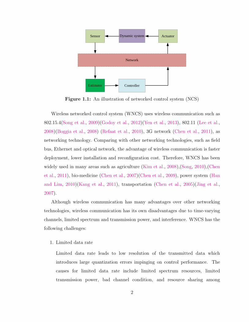
Dynamic systemSensor
Estimator
Actuator
Network
Controller
Figure 1.1: An illustration of networked control system (NCS)
Wireless networked control system (WNCS) uses wireless communication such as
802.15.4(Song et al., 2009)(Godoy et al., 2012)(Yen et al., 2013), 802.11 (Lee et al.,
2008)(Boggia et al., 2008) (Refaat et al., 2010), 3G network (Chen et al., 2011), as
networking technology. Comparing with other networking technologies, such as field
bus, Ethernet and optical network, the advantage of wireless communication is faster
deployment, lower installation and reconfiguration cost. Therefore, WNCS has been
widely used in many areas such as agriculture (Kim et al., 2008),(Song, 2010),(Chen
et al., 2011), bio-medicine (Chen et al., 2007)(Chen et al., 2009), power system (Han
and Lim, 2010)(Kang et al., 2011), transportation (Chen et al., 2005)(Jing et al.,
2007).
Although wireless communication has many advantages over other networking
technologies, wireless communication has its own disadvantages due to time-varying
channels, limited spectrum and transmission power, and interference. WNCS has the
following challenges:
1. Limited data rate
Limited data rate leads to low resolution of the transmitted data which
introduces large quantization errors impinging on control performance. The
causes for limited data rate include limited spectrum resources, limited
transmission power, bad channel condition, and resource sharing among
2

multiple users. For example, the maximum data rate of IEEE 802.15.4
is 250kbps. Even if some wireless technologies such as IEEE 802.11 can
provide high data rate transmission, with the increasing number of devices and
applications in WNCS, the effectively allocated data rate for each device is still
low.
2. Packet data corruption
Packet data corruption can not only introduce communication noise to control
system if packets with error are kept, but also increase packet transmission
delay due to retransmission and packet dropout. The causes for packet data
corruption are interference, fading, multi-path effects. For applications which
are not sensitive to delay, packet data corruption can be compensated by
retransmission. However, as pointed out by Mostofi and Murray (2009c)
some applications has stringent delay requirement. For such applications
retransmitted packets which miss deadline are useless.
3. Packet delay
The control system is sensitive to packet delay due to real time requirement.
However, the focus of research on communication side is the accuracy of
data transmission instead of packet delay. Packet delay includes network
access time (i.e., the interval between the transmitter receives the data and
transmitter starts to transmit over network) and packet transmission time (i.e.,
the interval between transmitter starts to transmit the data and transmitter
finish transmitting the data). The network access delay is due to resource
competition during multiple users, and is not guaranteed during network
congestion. The network transmission delay is due to transmission time over
medium, transmission error leading to multiple transmission, and transmission
over many hops.
4. Packet dropout
3
Modulation
Channel
coding
(optional)
Joint
decoding
System
state
estimation
Dynamic system
Sensor Processor
System stateSystem state
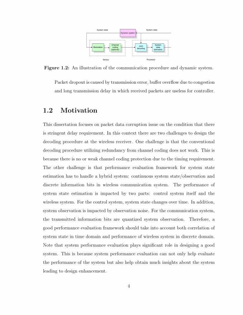
Figure 1.2: An illustration of the communication procedure and dynamic system.
Packet dropout is caused by transmission error, buffer overflow due to congestion
and long transmission delay in which received packets are useless for controller.
1.2 Motivation
This dissertation focuses on packet data corruption issue on the condition that there
is stringent delay requirement. In this context there are two challenges to design the
decoding procedure at the wireless receiver. One challenge is that the conventional
decoding procedure utilizing redundancy from channel coding does not work. This is
because there is no or weak channel coding protection due to the timing requirement.
The other challenge is that performance evaluation framework for system state
estimation has to handle a hybrid system: continuous system state/observation and
discrete information bits in wireless communication system. The performance of
system state estimation is impacted by two parts: control system itself and the
wireless system. For the control system, system state changes over time. In addition,
system observation is impacted by observation noise. For the communication system,
the transmitted information bits are quantized system observation. Therefore, a
good performance evaluation framework should take into account both correlation of
system state in time domain and performance of wireless system in discrete domain.
Note that system performance evaluation plays significant role in designing a good
system. This is because system performance evaluation can not only help evaluate
the performance of the system but also help obtain much insights about the system
leading to design enhancement.
4
We propose to exploit the redundancy in the system state, which can be considered
as a ‘nature encoding’ for the messages. A linear system model is adopted, where
x(t + 1) = Ax(t) + Bu(t) + n(t) is used to describe the dynamics of system state
x subject to the control u(t) and noise n(t). We observed that the system state is
similar to the convolutional codes except that the ‘encoding’ of the system state is
in the real field instead of the Galois field. Hence, the message actually has been
channel coded by the nature although no explicit or little explicit channel coding is
used at the transmitter.
1.3 Contributions
The contribution of this dissertation work can be summarized as follows:
Firstly, we propose to exploit the redundancy in the system state, which can be
considered as a ‘nature encoding’ for the messages. We use both schemes of Kalman
filtering and Pearl’s Belief Propagation (BP) for the soft decoding, combined with
the soft demodulation to improve the reliability of demodulation and decoding. A
practical dynamic system for electric generator dynamic system is used for numerical
simulation, which demonstrates the performance gain of incorporating the inherent
redundancy in the ‘nature encoding’. The procedure is illustrated in Figure 1.2. Note
that such a scheme is similar to the Turbo processing techniques like Turbo decoding
(Berrou et al., 1993), Turbo multiuser detection (Alexander et al., 1999) and Turbo
equalization (Tuchler et al., 2002) in wireless communication systems. However,
the ‘nature encoding’ is analog and implicit, thus resulting in a different processing
procedure.
Firstly, for systems with or without explicit channel coding, a decoding procedures
based on Pearl’s Belief Propagation (BP), in a similar manner to Turbo processing
in traditional data communication systems, is proposed. Numerical simulations have
demonstrated the validity of the schemes, using a linear model of electric generator
5

dynamic system. One disadvantage of this proposed scheme is that there is error
propagation at low SNR for uncoded system.
Secondly, we propose a quickest detection based error propagation detection
scheme to detect error propagation online. Then we combine this proposed error
propagation detection scheme with the proposed BP based channel decoding and
state estimation algorithm. The numerical results show that error propagation is
eliminated and consistent performance gain is observed in the proposed BP based
channel decoding and state estimation with protection of error propagation detection.
Finally, we propose to use MSE-based transfer chart to evaluate the performance of
BP based channel decoding and state estimation. We focus on two models, BP based
sequential and iterative channel decoding and state estimation. The first model is
used to evaluate the performance of sequential channel decoding and state estimation
over time slots; and the second model is used to evaluate the performance of iterative
channel decoding and state estimation over two time slots. The numerical results
show that MSE-based transfer chart can provide much insight about the performance
of the proposed BP based channel decoding and state estimation algorithm.
1.4 Dissertation Outline
The remainder of this dissertation is organized as follows. Literatures on the topics
listed above are surveyed in next chapter, chapter 2. Chapter 3,4 and 5 report main
work of this dissertation: a) chapter 3 presents the proposed BP based channel
decoding and state estimation procedure; b) chapter 4 shows the proposed error
propagation detection scheme and how to utilize it eliminate error propagation of
the proposed BP based channel decoding and state estimation scheme; c) chapter
5 demonstrates the proposed MSE-based transfer chart performance evaluation
framework and how to use it to evaluate the performance of proposed channel
decoding and system state estimation procedure. We conclude this dissertation, and
then outline future work in chapter 6.
6

Chapter 2
Literature Review
In this chapter we briefly review the existing works that are relevant to the topics
in this dissertation. Discussions include state estimation in NCS, evaluation for the
relationship between the operation of network and quality of control system, channel
coding and decoding and its performance evaluation in communication system.
2.1 State Estimation in NCS
The task of state estimation is to estimate system state at the remote controller side
by using information transmitted from plant over lossy network, which may corrupt,
delay, or drop transmitted information. The commonly used framework for state
estimation is shown in Figure 2.1. The output signals are measured by sensors at
given time, optionally processed by local processor, sent via digital network, recovered
by estimator at the remote controller side. Note that local processor at the plant side
is optional, and it requires extra computation capability at the plant side.
For the framework without local processor at the plant side, the measurement
of system observation is transmitted over the network. However, data may be
corrupted, delayed or dropped while being trasmitted over network. In most works,
it is assumed that erroneous packets are discarded at the estimator side. Therefore,
estimator receives only correctly received packets, and is impacted by packet dropout
7

SensingLocal
ProcessorDynamic System
Estimator
Network
Controller
Figure 2.1: State estimaton framework in NCS.
and packet transmission delay. The case with measurement transmission delay was
considered by (Alexander, 1991), (Larsen et al., 1998), (Nilsson et al., 1998), and
(Matveev and Savkin, 2003). Matveev and Savkin (2003) studied the case with
multiple sensors which independently transmit measurements to the estimator with
random delay. The case with packet dropout was discussed by (Nahi, 1969), (Sinopoli
et al., 2004), (Liu and Goldsmith, 2004), (Imer et al., 2006), in which the system
state can be estimated by using time-varying Kalman filter (TVTF). Sinopoli et al.
(2004) studied the performance of TVTF when the packet dropout pattern is an i.i.d
Bernoulli process. Liu and Goldsmith (2004) extended the results to the case with
partial observation loss, in which measurements of output signals are split into two
parts which are encoded separately, transmitted and dropped independently over two
wireless channels. One concern for TVTF is its complexity since matrices computation
has to be conducted online even for time invariant system. In order to avoid this
difficulty, Smith and Seiler (2003) proposed to pre-compute a finite set of parameters
which can be selected online according to the packet dropout history in the last
few time steps. Instead of linear optimal estimator, Ma et al. (2011) designed the
optimal estimator for the case with Bernoulli distribution of packet dropout. The
case with both packet dropout and delay was addressed by Schenato (2008) in which
the minimum error covariance estimator was derived. The case with packet dropout,
8

delay and measurement loss was addressd by Moayedi et al. (2010) in a probabilistic
manner.
All of the above mentioned works assume that measurement transmitted over
network is either accurately received or dropped. However, data corruption in wireless
communication happens a lot due to channel fading, interference. As pointed out by
Mostofi and Murray (2009c) some real-time application is more sensitive to packet
drop than data transmission error. Therefore, the stability of these applications can
be improved by accepting erroneous packets instead of discarding them. However,
keeping packets with transmission error increases communication noise. Mostofi and
Murray (2009c) (Mostofi and Murray, 2009b)(Mostofi and Murray, 2009a) discussed
the impact of keeping erroneous packets on estimation and identified the conditions to
keep or drop packets. Another issue, called unknown packet arrival issue, is observed
by Ma et al. (2009)(Ma et al., 2010)(Ma et al., 2012) while utilizing cognitive radio as
communication medium for WNCS. Cognitive radio is an intelligent communication,
in which secondary user keeps monitoring primary user’s spectrum usage in order
to look for spectrum holes. When primary user does not use the spectrum, then
secondary user can use the spectrum hole to transmit data; however, secondary user
cannot transmit when all spectrum is being used by primary users. Ma et al. (2009)
discussed the challenge of integrating cogntive raido into WNCS. Since the trasmission
of secondary user is impacted by spectrum usage of primary user; therefore, the
transmission of measurement from sensor is intermittent; in addition, the estimator
may not know if packet including measurement is trasmitted or not in current time
slot, which is called unknown packet arrival issue. Therefore, estimator has to decide
if the received signal contains trasmitted data from sensor or just noise. Ma et al.
(2009)(Ma et al., 2010)(Ma et al., 2012) designed the estimation algorithm which
takes into account this unknown packet arrival issue introduced by cognitive radio.
The framework with local estimation was studied by Xy and Hespanha (2005),
Gupta et al. (2009), and Xu and Hespanha (2004). In this framework, the sensor
can also preprocess the measurements to obtain estimates of output signal; then the
9

estimate of output signals instead of raw measurement is sent to remote estimator.
The main advantage of this solution is that every successfully received message at
the remote estimator includes all relevant information that can be extracted from
all previous raw measurements. Therefore, this framework is more robust to packet
drop than the framework without local estimation. Gupta et al. (2009) derived the
optimal estimation framework which can handle any packet-dropping process. In
addition, when network condition is good sensor can choose to not send estimates
to remote estimator to reduce traffic while estimation performance is not degraded.
Following this perspective many works have been conducted to explore the balance
between communication and estimation performance (Xu and Hespanha, 2004)(Xu
and Hespanha, 2005) and (Yook et al., 2002).
Another method to improve the performance of estimation is multi-sensor state
estimation, in which multiple sensors are used to measure the dynamic system
and their measurement results are co-used to estimate system state. As pointed
out by Duan et al. (2007), multi-sensor state estimation is potential in improving
estimation accuracy, extending observability and coverage, enhancing survivability
and reliability. Many estimation fusion technologies including centralized fusion and
distributed fusion are proposed to efficiently aggregate measurements from multiple
sensors (Chiuso and Schenato, 2008), (Duan and Li, 2011), (Liu et al., 2012).
One more perspective to improve the performance of state estimation is to
control the network. For instance, Quevedo et al. (2010) and Quevedo et al. (2013)
proposed to dynamically control power and coding scheme at the transmitter in order
to maintain channel quality while saving energy. Gupta et al. (2006),Mo et al.
(2011),Yang et al. (2013) discussed about the sensor scheduling method in order
to solve communication competition among sensors. Many fusion technologies are
proposed by (Chiuso and Schenato, 2008), (Duan and Li, 2011), (Liu et al., 2012) to
efficiently aggregate measurements from multiple sensors. Bai et al. (2012) proposed
the cross-layer adaptive sampling rate and network scheduling. Chamaken and Litz
10
(2010) used a practical case study to demonstrate the performance improvement and
efficiency of jointly designing control and communication system.
2.2 Evaluation for Relationship between the Op-
eration of Network and Quality of Control
System
In this section, we briefly introduce the relative works which explore the condition
for stability with quantization error, packet drop and packet transmission delay.
2.2.1 Data Rate Therorem
The aim of data rate theorem is to determine how much rate is necessary to construct
a stabilizing quantizer/controller pair in order to cope with the challenge of limited
bandwidth in NCS. Data rate theorem is analogous to Shannon’s source coding theory
in communication theory, which aims to determine the lowest data rate above which a
give random process can be communicated with arbitrarily small probability of errors
(Shannon, 1948)(Cover and Thomas, 1991). However, source coding theory allows the
usage of arbitrarily long codes leading to unbounded transmission delay and breakage
of causality of the system. Therefore source coding theory is not applicable for control
system due to that close-loop feedback control in control system requires that data
transmission has to be causal and real-time.
The widely used plant model for the research of data rate theorem is an unstable
linear dynamical system. The output signals are measured at fixed sampling interval,
quantized, encoded, and sent to decoder at the controller side over a noiseless digital
link. One special constraint is that both encoder at the system side and decoder at
the controller have only causal knowledge of channel state, i.e., current supported
data rate. The simplified case of constant data rate was addressed by Tatikonda and
11

Mitter (2004) and Nair and Evans (2004). The case with a time-varying independent
and identically distributed (i.i.d.) rate process was considered by Martins et al. (2006)
and Minero et al. (2009). Since the wireless channel is temporally correlated, the case
of Markov rate process which has one state with channel rate 0 and the other state
with constant channel rate was studied by You and Xie (2011). Finally, Minero et al.
(2013) derived data rate theorem for general case with Markov channel rate process.
This result can also be used to derive the data rate theorem for many special test
cases, such as constant channel rate, time-varying i.i.d. channel rate process.
2.2.2 Packet Dropout Rate
The task of stability analysis for packet dropout is to find out the critical packet
dropout rate above which no control scheme can stabilize the system. In this context,
the output signals of the plant are sampled, encoded as a packet, and transmitted
over network. Quantization effect is ignored, and a packet carries whole information
of sampled output signals. However, packets may be dropped due to transmission
error from physical layer especially wireless communication, buffer overflow due to
congestion, and long transmission delay.
The case with i.i.d Bernoulli packet dropout pattern were addressed by Sinopoli
et al. (2004) and Gupta et al. (2007a). The case with Markov packet drop process
including bad state, i.e., over which packet is dropped over network, and good state,
i.e., over which packet is successfully delivered, was studied by Gupta et al. (2007b).
Note that the results for data rate theorem can also be used to derive the critical
packet dropout rate over which system cannot be stabilized by any control scheme.
Minero et al. (2009) recovered that packet loss model can be represented by model
for data rate theorem, i.e., by letting the rate take value 0 and ∞.
12
2.2.3 Sampling and Delay
To transmit continuous signal over digital communication network, the transmitter
has to sample the continuous signal, and then encode it and send it to receiver over
transmission medium. Then the receiver decodes the transmitted signal. In digital
control, the interval between two samples at the receiver is equal to the sampling
interval. However, in NCS the interval between two samples is impacted by sampling
interval, network access time (i.e., the interval between the transmitter receives the
data and transmitter starts to transmit over network) and packet transmission time
(i.e., the interval between transmitter starts to transmit the data and transmitter
finishs transmitting the data). In addition, the network access time and packet
transmission time are variable, which are dependent on network traffic condition
and channel quality, respectively.
One case is one-channel feedback NCS, in which plant is modeled as a continuous-
time linear time-invariant system (LTI). The output signal is sampled and sent over
the communication network to the controller. The interval between two receiving
sampled output signals at the controller is impacted by sampling interval, network
access time, packet transmission time, and packet dropout. Before the arrival of next
sampled output signal, the value of last received sampled output signal is held as
constant and used to make decision for actions. The case with periodic-sampling
and fixed delay was considered by Branicky et al. (2000), and Zhang et al. (2001)
concluded the sufficient condition for the stability of LTI NCS by referring to the
results for nonlinear hybrid system (Branicky, 1997). Since the delays in most cases
are not constant, the case with variable delay has also drawn attentions. Lin et al (Lin
et al., 2003)(Lin and Antsaklis, 2004)(Lin and Antsaklis, 2005) addressed one special
case of periodic sampling and variable delay, in which computation and transmission
time can be ignored, and the main source of delay is network access time. Lin et al.
(2003) discretized delay and concluded the condition for stability by using average
dwell time results for discrete switched systems (Zhai et al., 2002). The case with
13
variable sampling interval or variable delay is most chanllenging . Zhang and Branicky
(2001) expressed the sufficient conditions for its stability as a a Lyapunov function.
However, it is generally not simple to solve this Lyapunov function in order to check if
a given interval for sampling and delay is stable or not. They proposed a randomized
algorithm to find the largest value of sampling interval for the stability of a special
case in which the minimum sampling is 0 and there is no delay.
Another case for stability analysis is model-based networked control system (MB-
NCS), which is introduced by Montestruque and Antsaklis (2002a). The main purpose
of MB-NCS is to reduce the amount of data exchange in network, by making use of
model of the plant at the controller. More specifically, most of time the system
is controlled with open-loop mode in which actions are made based on the plant
model at the controller. The model of plant at the controller is updated at fixed
interval by using close-loop mode. Comparing with one-channel feedback NCS in
which last data received from network is held constant, MB-NCS instantaneously
updates the state of controller after receiving data from network. Montestruque
and Antsaklis (Montestruque and Antsaklis, 2002a)(Montestruque and Antsaklis,
2002b)(Montestruque and Antsaklis, 2003a) first derived the maximum value of
periodic sampling interval for which the NCS is still stable; then they considered
the case with stochastic sampling interval. The stability condition for i.i.d sampling
interval was considered in (Montestruque and Antsaklis, 2003b); then the results was
further generalized to Markov sampling intervals in (Montestruque and Antsaklis,
2004).
A general nonlinear case was addressed by Walsh et al. (2002) and Nesic and Teel
(2004), where a nonlinear plant and remote controller are impacted by exogenous
disturbances. Both control signals and output signals are sampled and transmitted
over network. Between sampling times, the data for control signals and output signals
are held constant at the actuator and controller, respectively. In addition, it is allowed
to transmit a portion of entries of control signals and output signals at given sampling
14
times. This can be used to capture some network access protocols by which only a
part of control signals and output signals can be transmitted in the given time.
2.3 Channel Coding and Decoding
The development of channel coding and decoding has split into two paths. One
category is that source coding and decoding are not taken into account while designing
channel coding and decoding. This is guided by the separation principle, which
states there is no gain from joint data compression and channel transmission. Due to
the independence of source many diverse source can share the same coding scheme.
Therefore, many coding schemes have been wildly used, such as convolutional code
(Elias, 1955), turbo code (Heegard and Wicker, 1999), serially concatenated code
(Benedetto et al., 1998) and LDPC code (Gallager, 1963).
However, separation principle holds only when channels are stationary and there
is no delay requirement for sources (Vembu et al., 1995). For fixed length blocks,
there is redundancy in source no matter if source is encoded or not. Therefore, the
redundancy in source drives the development of joint source decoding and channel
coding. There are two models to describe the redundancy left in the source. One
model is based on the high level information from the source, and is highly dependent
on the source (Yin et al., 2002; Mei and Wu, 2006; Pan et al., 2006; Pu et al., 2007;
Ramzan et al., 2007). The other model for redundancy from source is Markov source
(Garcia-Frias and Villasenor, 1997, 1998, 2001; Garcia-Frias and Zhao, 2001, 2002;
Garcia-Frias and Zhong, 2003; Garcia-Frias et al., 2003; Fresia et al., 2010). The
advantage of Markov model is that the parameters do not have to be known at the
receiver side. Garcia-Frias and Villasenor (1998, 2001) extended the joint source
coding and channel decoding for Markov model with unknown parameters. Zhao and
Garcia-Frias (2002, 2005) extended it to non-binary source.
15
2.4 Performance Analysis For Channel Decoding
The purpose of performance analysis for iterative decoding scheme is to find out for a
given codec and decoder, for which kind of channel noise power the message-passing
decoder can correct the errors or not. Then the results of performance analysis can
be used to assist the design of codec and decoder.
Gallager (1963) proposed to use density evolution to track the iterative decoding
performance. It is based on the assumption that, for very long codes, the extrinsic
LLRs passed between the component decoders are independent and identically
distributed. Then, for the iterative decoding performance it is equivalent to track the
evolution of extrinsic LLRs probability density functions through iterative decoding
process.
ten Brink (1999, 2000, 2001) proposed to use extrinsic information transfer chart
(EXIT) to track the iterative decoding performance. Based on the assumption
that the distribution of extrinsic log-likelihood ratio (LLR) is Gaussian EXIT tracks
mutual information of extrinsic LLRs instead of density evolution. Comparing with
density evolution, the computation for EXIT is simplified. In addition, the evolution
of mutual information through iterative decoding process can be illustrated in a graph
and easy to visualize. EXIT has two properties. One property is that for convergence
of iterative decoding, the flipped EXIT curve of the outer decoder should lie below the
EXIT curve of the inner coder. The other property is that the area under EXIT curve
of outer code relates to the rate of inner coder. Ashikhmin et al. (2004) demonstrated
that if the a priori channel is an erasure channel, for any outer code of rate R, the
area under the EXIT curve is 1−R. To the best knowledge of us, the area property
of EXIT has been proved only for erasure priori channel.
Instead of tracking mutual information MSE is proposed to track the iterative
decoding performance (Bhattad and Narayanan, 2007). The MSE-based chart
analysis method is based on the relationship between mutual information and
minimum mean square error (MMSE) in AWGN channel (Guo et al., 2005). Bhattad
16
and Narayanan (2007) has proven the area property of MSE chart when the priori
channel is Gaussian.
The difference of iterative channel decoding and state estimation in our work is
that we have a hybrid model. The system state and observation are non-binary source
in continuous domain; on the other hand the information transmitted in wireless
system is quantized bits. Therefore, the method proposed in (Guo et al., 2005) cannot
be used directly. The key challenge is how to handle the message transfer between
non-binary source and information bits. The other difference is that the source is
correlated over time. The estimation error from previous time slots also affects the
performance of estimation in current time slots. Therefore, besides evaluating the
performance of iterative channel decoding and state estimation in two time slots, it
is also very important to evaluate the performance of state estimation over time.
Another area in wireless communication related to our work is joint source and
channel decoding (Yin et al., 2002; Mei and Wu, 2006; Pan et al., 2006; Pu et al.,
2007; Ramzan et al., 2007; Garcia-Frias and Villasenor, 1997, 1998, 2001; Garcia-Frias
and Zhao, 2001, 2002; Garcia-Frias and Zhong, 2003; Garcia-Frias et al., 2003). The
idea of joint source and channel decoding is to utilize redundancy in source to assist
channel decoding. Our work can also be considered as one special case of joint source
and channel decoding. However, there are two major differences. One difference is
that most works focus on binary source and EXIT chart was used for performance
analysis (Fresia et al., 2010). Zhao and Garcia-Frias (2002, 2005) considered the case
with non-binary source, but the performance analysis was not provided. The other
difference is these works considered the joint source and channel decoding over only
two time slots. In our work, the dynamic state changes over time. Therefore, the
performance of channel decoding and system estimation at the current time slots also
impacts its performance in the future. Therefore, we also study the performance of
iterative estimation and decoding over time.
17
Chapter 3
Decoding the ‘Nature Encoded’
Messages for Wireless Networked
Control System
3.1 Introduction
In this chapter, we study the decoding procedure (including the demodulation
procedure) for the messages with no or weak channel coding protection in the context of
wireless networked control system (WNCS). The key point is to exploit the redundancy
in the system state, which can be considered as a ‘nature encoding’ for the messages.
In this work, a linear system model is adopted, where x(t+1) = Ax(t)+Bu(t)+n(t)
is used to describe the dynamics of system state x subject to the control u(t) and noise
n(t). We observe that the system state is similar to the convolutional codes except
that the ‘encoding’ of the system state is in the real field instead of the Galois field.
Hence, the message actually has been channel coded by the nature although no explicit
or little explicit channel coding is used at the transmitter. We use both schemes of
Kalman filtering and Pearl’s Belief Propagation (BP) for the soft decoding, combined
with the soft demodulation to improve the reliability of demodulation and decoding.
18

Modulation
Channel
coding
(optional)
Joint
decoding
System
state
estimation
Dynamic system
Sensor Processor
System stateSystem state
Figure 3.1: An illustration of the communication procedure and dynamic system.
An electric generator dynamic system will be used for numerical simulation, which
demonstrates the performance gain of incorporating the inherent redundancy in the
‘nature encoding’. The procedure is illustrated in Figure 3.1. Note that such a scheme
is similar to the Turbo processing techniques like Turbo decoding (Berrou et al., 1993),
Turbo multiuser detection (Alexander et al., 1999) and Turbo equalization (Tuchler
et al., 2002) in wireless communication systems. However, the ‘nature encoding’ is
analog and implicit, thus resulting in a different processing procedure.
The remainder of this chapter is organized as follows. The system model is
introduced in Section 3.2. The decoding procedure is discussed for the schemes of
Kalman filtering based heuristic approach and the BP approach in Sections 3.3 and
3.4, respectively. Numerical simulation results are shown in Section 3.5. Finally, the
conclusions are drawn in Section 3.6.
3.2 System Model
3.2.1 Linear System
We consider a discrete time linear dynamic system, whose system state evolution is
given by x(t+ 1) = Ax(t) + Bu(t) + n(t),
y(t) = Cx(t) + w(t), (3.1)
19
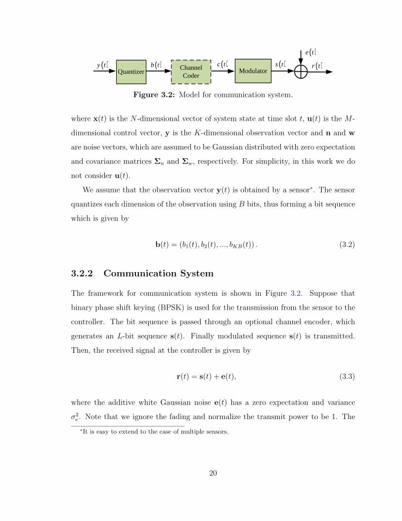
QuantizerChannel Coder
( )y t ( )b t
( )e t
( )r t( )c tModulator
( )s t
Figure 3.2: Model for communication system.
where x(t) is the N -dimensional vector of system state at time slot t, u(t) is the M -
dimensional control vector, y is the K-dimensional observation vector and n and w
are noise vectors, which are assumed to be Gaussian distributed with zero expectation
and covariance matrices Σn and Σw, respectively. For simplicity, in this work we do
not consider u(t).
We assume that the observation vector y(t) is obtained by a sensor∗. The sensor
quantizes each dimension of the observation using B bits, thus forming a bit sequence
which is given by
b(t) = (b1(t), b2(t), ..., bKB(t)) . (3.2)
3.2.2 Communication System
The framework for communication system is shown in Figure 3.2. Suppose that
binary phase shift keying (BPSK) is used for the transmission from the sensor to the
controller. The bit sequence is passed through an optional channel encoder, which
generates an L-bit sequence s(t). Finally modulated sequence s(t) is transmitted.
Then, the received signal at the controller is given by
r(t) = s(t) + e(t), (3.3)
where the additive white Gaussian noise e(t) has a zero expectation and variance
σ2e . Note that we ignore the fading and normalize the transmit power to be 1. The
∗It is easy to extend to the case of multiple sensors.
20
algorithm and conclusion in this work can be easily extended to the case with different
types of fading.
3.3 Kalman Filtering based Heuristic Approach
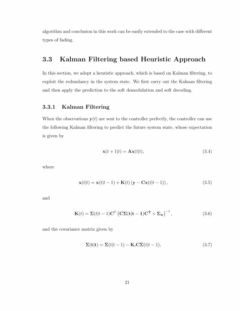
In this section, we adopt a heuristic approach, which is based on Kalman filtering, to
exploit the redundancy in the system state. We first carry out the Kalman filtering
and then apply the prediction to the soft demodulation and soft decoding.
3.3.1 Kalman Filtering
When the observations y(t) are sent to the controller perfectly, the controller can use
the following Kalman filtering to predict the future system state, whose expectation
is given by
x(t+ 1|t) = Ax(t|t), (3.4)
where
x(t|t) = x(t|t− 1) + K(t) (y −Cx(t|t− 1)) , (3.5)
and
K(t) = Σ(t|t− 1)CT(CΣ(t|t− 1)CT + Σw
)−1, (3.6)
and the covariance matrix given by
Σ(t|t) = Σ(t|t− 1)−KtCΣ(t|t− 1), (3.7)
21
where
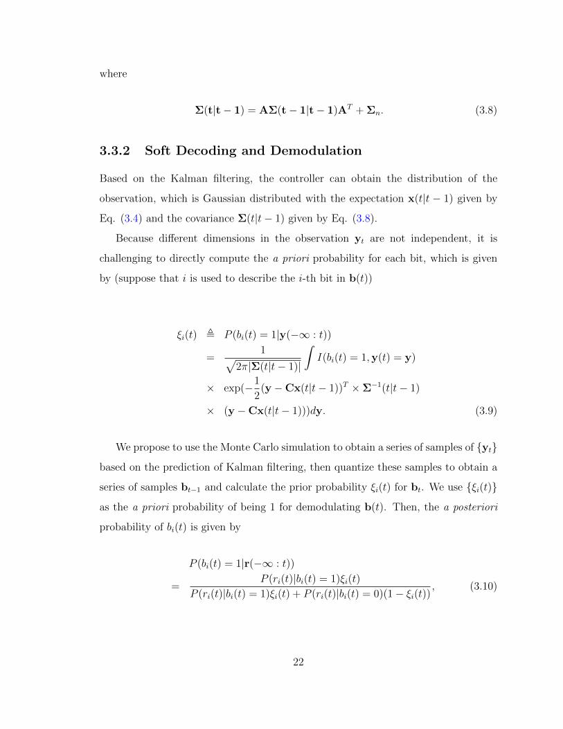
Σ(t|t− 1) = AΣ(t− 1|t− 1)AT + Σn. (3.8)
3.3.2 Soft Decoding and Demodulation
Based on the Kalman filtering, the controller can obtain the distribution of the
observation, which is Gaussian distributed with the expectation x(t|t − 1) given by
Eq. (3.4) and the covariance Σ(t|t− 1) given by Eq. (3.8).
Because different dimensions in the observation yt are not independent, it is
challenging to directly compute the a priori probability for each bit, which is given
by (suppose that i is used to describe the i-th bit in b(t))
ξi(t) , P (bi(t) = 1|y(−∞ : t))
=1√
2π|Σ(t|t− 1)|
∫I(bi(t) = 1,y(t) = y)
× exp(−1
2(y −Cx(t|t− 1))T ×Σ−1(t|t− 1)
× (y −Cx(t|t− 1)))dy. (3.9)
We propose to use the Monte Carlo simulation to obtain a series of samples of {yt}
based on the prediction of Kalman filtering, then quantize these samples to obtain a
series of samples bt−1 and calculate the prior probability ξi(t) for bt. We use {ξi(t)}
as the a priori probability of being 1 for demodulating b(t). Then, the a posteriori
probability of bi(t) is given by
P (bi(t) = 1|r(−∞ : t))
=P (ri(t)|bi(t) = 1)ξi(t)
P (ri(t)|bi(t) = 1)ξi(t) + P (ri(t)|bi(t) = 0)(1− ξi(t)), (3.10)
22
P (ri(t)|bi(t) = 1) =1√
2πσ2e
exp
(−(ri(t)− 1)2
2σ2e
). (3.11)
P (ri(t)|bi(t) = 0) =1√
2πσ2e
exp
(−(ri(t) + 1)2
2σ2e
). (3.12)
Note that the Kalman filtering is no longer rigorous in the networked control
system due to the quantization error and possible decoding error. The proposed
heuristic approach is based on the assumption that the Kalman filtering is very
precise. As will be shown in the numerical results, this approach will be seriously
affected by the propagation of decoding errors.
3.4 BP based Iterative Decoding
In this section, we consider the iterative decoding using BP with the mechanism of
message passing between the system state and received signals. The key observation
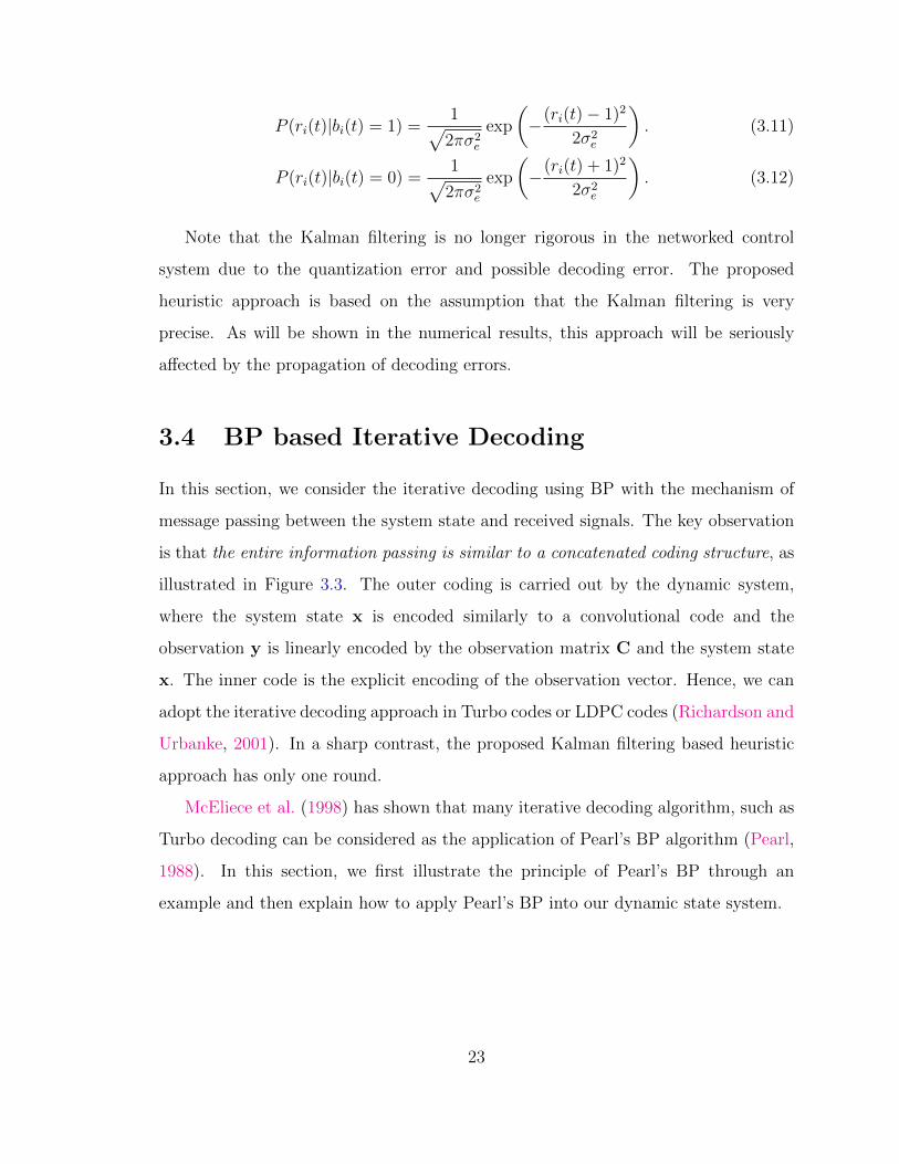
is that the entire information passing is similar to a concatenated coding structure, as
illustrated in Figure 3.3. The outer coding is carried out by the dynamic system,
where the system state x is encoded similarly to a convolutional code and the
observation y is linearly encoded by the observation matrix C and the system state
x. The inner code is the explicit encoding of the observation vector. Hence, we can
adopt the iterative decoding approach in Turbo codes or LDPC codes (Richardson and
Urbanke, 2001). In a sharp contrast, the proposed Kalman filtering based heuristic
approach has only one round.
McEliece et al. (1998) has shown that many iterative decoding algorithm, such as
Turbo decoding can be considered as the application of Pearl’s BP algorithm (Pearl,
1988). In this section, we first illustrate the principle of Pearl’s BP through an
example and then explain how to apply Pearl’s BP into our dynamic state system.
23
ModulationChannel
coding
System
state
System
observation
Outer code
Inner code
Coded bit
sequence
System dynamics
Sensing
Figure 3.3: An illustration of the coding structure.
( )mXU Um ,π ( )XXYn ,λ
Figure 3.4: Message Passing of BP.
24
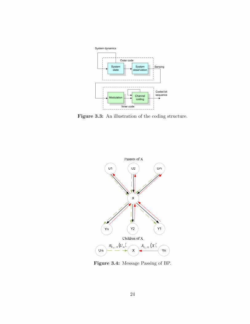
3.4.1 Introduction of Pearl’s BP
As shown in Figure 3.4, random variable X has parents U1, U2, · · · , UM and children
Y1, Y2, · · · , YN . The message passing of Pearl’s BP is indicated by green arrows and
red arrows in the figure. Green arrows transmit π-message which is sent from parent
to its children. For instance, the message passing from Um to X is πUm,X(Um), which
is the prior information of Um conditioned on all the information Um has received.
Red arrows transmit λ-message which is from children to its parent. For instance,
the message passing from Yn to X is λYn,X(X), which is the likelihood of X based
on the information Yn has received. After X receives all π-message πUm,X(Um)
from its parents U1, U2, · · · , UM and all λ-message λYn,X(X), X from its children
Y1, Y2, · · · , YN , X updates its belief information BELX(x) and transmits λ-messages
λX,Um(Um) to its parents and π-message πX,Yn(x) to its children. The expressions of
the quantities are given by
πX(x) =∑U
p(x|U)M∏m=1
πUm,X(Um) (3.13)
γX(U) =∑
x
N∏n=1
λYn,X(x)p(x|U) (3.14)
BELX(x) = α×N∏n=1
λYn,X(x)× πX(x) (3.15)
λX,Um(Um) =∑
U, 6=Um
γX(U)×∏j 6=m
πUj ,X(Uj) (3.16)
πX,Yn(x) = πX(x)×∏i 6=n
λYi,X(x) (3.17)
where U = (U1, U2, · · · , UM) and Y = (Y1, Y2, · · · , UN)
In the initialization procedure of Pearl’s BP, some initial values are needed for the
running of Pearl’s BP. The initial values are defined as
λX,U(u) =
p(x0|u), Xis evidence,x = x0
1, Xis not evidence, (3.18)
25
and
πX,Y (x) =
δ(x,x0), Xis evidence,x = x0
p(x), X is source, not evidence. (3.19)
3.4.2 Application of Pearl’s BP in NCS
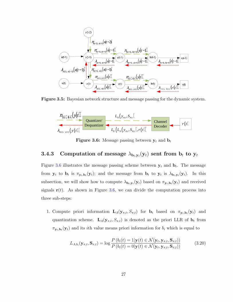
The Bayesian network structure of the control system and communication system in
the NCS is shown for three time slots in Figure 3.5. In the Bayesian network, the
system state xt is dependent on the previous system state xt−1 and the control action
ut; the observation yt is dependent on the system state xt; the uncoded bits bt are
dependent on the observation vector yt; the received signal rt is dependent on the
uncoded bits bt. Here we omit the coded bits st as the relationship between the
uncoded bits bt and the coded bits st is deterministic. Figure 3.5 shows the Bayesian
Network structure for the dynamic system with three observations: xt−2, xt−1 and
xt.
Based on the Bayesian network structure, the iterative decoding procedure can
be derived. Figure 3.5 shows the message passing in the dynamic system. xt−2
summarizes all the information obtained from previous time slots and transmits
π-message πxt−2,xt−1(xt−2) to xt−1. The BP procedure can be implemented in
synchronous or asynchronous manners. As the decoding process has a large overhead,
we implement asynchronous Pearl’s BP. The updating order and message passing in
one iteration is as follows: step 1): xt−1 Õ yt−1; step 2): yt−1 Õ bt−1; step 3): bt−1 Õ
yt−1; step 4): yt−1 Õ xt−1; step 5): xt−1 Õ xt; step 6): xt Õ yt; step 7): yt Õ bt; step
8): bt Õ yt; step 9): yt Õ xt; step 10): xt Õ xt−1; step 11): xt−1 updates information.
The detailed mathematical derivation for each step is shown in Appendix A.1 and
the messaging passing between y(t) and b(t) is shown in next subsection.
26
( )( )1)1(),1( −−− txtytxπ ( )( )1)1(),1( −−− tytbtyπ
( )( )1)1(),1( −−− tytytbλ( )( )1)1(),1( −−− txtxtyλ
( ))2()1(),2( −−− txtxtxπ
( )( )1)1(),1( −−− trtbtrλ
( )( )txtytx )(),(π ( ) ( ) ( )( )tytbty ,π
( )( )tytytb )(),(λ( )( )txtxty )(),(λ
( ))1()(),1( −− txtxtxπ
( )( )trtbtr )(),(λ
( ))1()1(),( −− txtxtxλ
Figure 3.5: Bayesian network structure and message passing for the dynamic system.
( )( )( ), ( )b t y t y tλ
Channel Decoder
Quantizer/Dequantizer
( ), ,,A t tL y Sπ π
( ) ( )( ), ,, ,E A t tL L y S r tπ π
( ) ( ) ( )( )tytbty ,π( )r t
Figure 3.6: Message passing between yt and bt
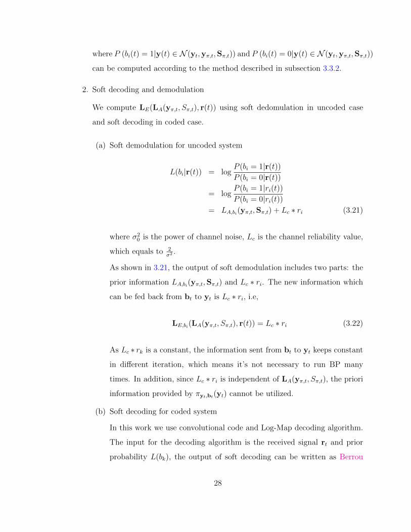
3.4.3 Computation of message λbt,yt(yt) sent from bt to yt
Figure 3.6 illustrates the message passing scheme between yt and bt. The message
from yt to bt is πyt,bt(yt); and the message from bt to yt is λbt,yt(yt). In this
subsection, we will show how to compute λbt,yt(yt) based on πyt,bt(yt) and received
signals r(t). As shown in Figure 3.6, we can divide the computation process into
three sub-steps:
1. Compute priori information LA(yπ,t, Sπ,t) for bt based on πyt,bt(yt) and
quantization scheme. LA(yπ,t, Sπ,t) is denoted as the priori LLR of bt from
πyt,bt(yt) and its ith value means priori information for bi which is equal to
LA,bi(yπ,t,Sπ,t) = logP (bi(t) = 1|y(t) ∈ N (yt,yπ,t,Sπ,t))
P (bi(t) = 0|y(t) ∈ N (yt,yπ,t,Sπ,t))(3.20)
27
where P (bi(t) = 1|y(t) ∈ N (yt,yπ,t,Sπ,t)) and P (bi(t) = 0|y(t) ∈ N (yt,yπ,t,Sπ,t))
can be computed according to the method described in subsection 3.3.2.
2. Soft decoding and demodulation
We compute LE(LA(yπ,t, Sπ,t), r(t)) using soft dedomulation in uncoded case
and soft decoding in coded case.
(a) Soft demodulation for uncoded system
L(bi|r(t)) = logP (bi = 1|r(t))
P (bi = 0|r(t))
= logP (bi = 1|ri(t))P (bi = 0|ri(t))
= LA,bi(yπ,t,Sπ,t) + Lc ∗ ri (3.21)
where σ20 is the power of channel noise, Lc is the channel reliability value,
which equals to 2σ2 .
As shown in 3.21, the output of soft demodulation includes two parts: the
prior information LA,bi(yπ,t,Sπ,t) and Lc ∗ ri. The new information which
can be fed back from bt to yt is Lc ∗ ri, i.e,
LE,bi(LA(yπ,t, Sπ,t), r(t)) = Lc ∗ ri (3.22)
As Lc ∗ rk is a constant, the information sent from bt to yt keeps constant
in different iteration, which means it’s not necessary to run BP many
times. In addition, since Lc ∗ ri is independent of LA(yπ,t, Sπ,t), the priori
information provided by πyt,bt(yt) cannot be utilized.
(b) Soft decoding for coded system
In this work we use convolutional code and Log-Map decoding algorithm.
The input for the decoding algorithm is the received signal rt and prior
probability L(bk), the output of soft decoding can be written as Berrou
28

et al. (1993):
L(bk|rt) = logP (bk = 1|rt)P (bk = 0|rt
= LA,bi(yπ,t,Sπ,t) + Lcrks + Le(bk) (3.23)
Therefore, the information which needs to be fed from bt to yt is Lcrks +
Le(bk), i.e.,
LE,bi(LA(yπ,t, Sπ,t), r(t)) = Lcri(t) + Le(bi) (3.24)
3. Compute λbt,yt(yt) from LE(LA(yπ,t, Sπ,t), r(t))
Based on LE(LA(yπ,t, Sπ,t), r(t)), b(t) can be estimated as (Bhattad and
Narayanan, 2007):
bi(t) =1
2tanh
(1
2LE,bi (LA(yπ,t,Sπ,t), r(t))
)+
1
2(3.25)
and MMSE in estimating bi(t) is given by
mmse (bi(t)|LA(yπ,t,Sπ,t), r(t))
=1
4− 1
4tanh2
(1
2LE,bi (LA(yπ,t,Sπ,t), r(t))
)(3.26)
Then, y(t) can be estimated:
yk(t) =B∑i=1
Qi−1I b(k−1)B+i(t)−
Qmax −Qmin
2(3.27)
29
and MMSE in estimating y(t) is given by:
mmse (yk(t)|LA(yπ,t,Sπ,t), r(t))
=B∑i=1
Q2(i−1)I mmse
(b′(k−1)B+i(t)|LA(yπ,t,Sπ,t), r(t)
)(3.28)
where [Qmin, Qmax] is the range for quantization, QI is the quantization interval,
which is given by:
QI =Qmax −Qmin
2B − 1(3.29)
We assume that the distribution of estimated y(t) is Gaussian, i.e.,
λbt,yt(yt) = N (yt,yλ,t, Sλ,t) (3.30)
where yλ,t is the mean which is equal to
yλ,t = [y1(t), · · · , yK(t)] (3.31)
and Sλ,t is the covariance matrix which is diagonal and its kth element is equal
to
Sk,kλ,t = mmse (yk(t)|LA(yπ,t,Sπ,t), r(t)) (3.32)
3.5 Numerical Simulations
In this section, we use numerical simulations to demonstrate the algorithms proposed
in this chapter.
We consider an electric generator dynamic system in which the system state is a
7-dimensional vector. The system is in the continuous time. The system dynamics
30

is described by a differential equation x(t) = A′x(t), where the matrix A′ is given
by (3.20) (Example 12.9 in (Machowski et al., 2008)). The physical meanings of the
system states are given in Table 3.1. For simplicity, we assume that the system is
unregulated, i.e., B = 0, and the sensor can sense the system state directly, i.e.,
C = I. We approximate the continuous time system using the discrete time system
with a small step size δt. Therefore, the matrix A in the discrete time system is given
by A = I + δtA′.
Table 3.1: Physical Meaning of System States
x1,x2 rotor swingsx3 excitation circuitx4 damping circuit in the d-axis and excitation circuitx5 damping circuit in the q-axisx6 voltage controller and excitation circuitx7 voltage controller
We run the simulations using Matlab to compare the performances of Kalman
filtering and Pearl’s BP based algorithms for systems with and without channel
coding. The baseline approach is the separated Kalman filtering and decoding process.
In the following, these three algorithms are referred as ‘KF Prior’, ‘BP’ and ‘KF’,
respectively. The performance metrics are the mean square error (MSE) of each
sample and the average bit error rate (BER). Each simulation runs 1000 times slots.
The configuration for both systems are as follows: for the dynamic system of power
system described in (3.1): δt = 0.01, Σn = 0.05 , Σw = 0.05. Each dimension of
the observation yt is quantized with 16 bits, and the dynamic range for quantization
is [−200, 200]. A 1/2 rate Recursive Systematic Convolutional (RSC) code is used
as the channel coding scheme; and the code generator is g = [1, 1, 1]. The decoding
algorithm is Log-Map algorithm.
31
A′ =
0 1 0 0 0 0 0−20.316 0 0 −25.048 −1.411 0 0−0.061 0 −0.773 −0.083 0.018 15.06 30.12−0.213 0 7.050 −5.026 0.063 0 0−2.654 0 0 −1.463 −12.958 0 0
0 0 0 0 0 0 1−0.008 0 0 −0.565 0.971 −3.33 −33.33
(3.20)
1 2 3 4 5 6 710
−2
10−1
100
101
102
103
104
105
EbN0: dB
MM
SE
KFKF PriorBP
Figure 3.7: Mean Square Error comparison for system without channel coding
3.5.1 Uncoded Case
Figures 3.7 and 3.8 show the simulation results for the uncoded case with different
Eb/N0. The performance of ’BP’ is the best; however, the performance of ’KF Priori’
is worse than ’KF’. The reason for the bad performance of ’KF Prior’ is:
1. The MSE of the estimate of y(t) is not transferred to estimator, then, the
statistics of communication noise is unknown to estimator. However, both
estimator and channel decoder are not aware that the estimated performance
32
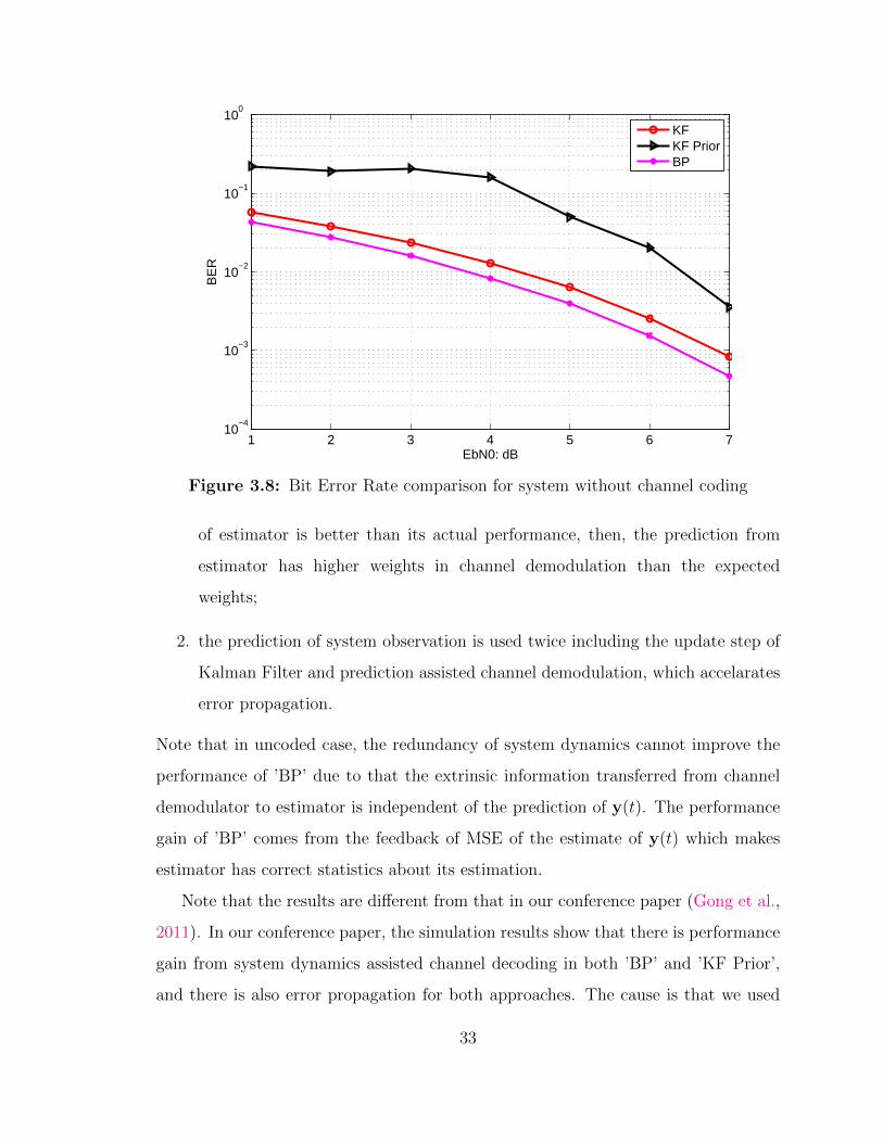
1 2 3 4 5 6 710
−4
10−3
10−2
10−1
100
EbN0: dB
BE
R
KFKF PriorBP
Figure 3.8: Bit Error Rate comparison for system without channel coding
of estimator is better than its actual performance, then, the prediction from
estimator has higher weights in channel demodulation than the expected
weights;
2. the prediction of system observation is used twice including the update step of
Kalman Filter and prediction assisted channel demodulation, which accelarates
error propagation.
Note that in uncoded case, the redundancy of system dynamics cannot improve the
performance of ’BP’ due to that the extrinsic information transferred from channel
demodulator to estimator is independent of the prediction of y(t). The performance
gain of ’BP’ comes from the feedback of MSE of the estimate of y(t) which makes
estimator has correct statistics about its estimation.
Note that the results are different from that in our conference paper (Gong et al.,
2011). In our conference paper, the simulation results show that there is performance
gain from system dynamics assisted channel decoding in both ’BP’ and ’KF Prior’,
and there is also error propagation for both approaches. The cause is that we used
33
different initial simulation condition. In our conference paper, at time slot 1 estimator
has perfect information of system state. Therefore, on one hand the estimator has
good prediction of system state which can help improve the performance of channel
decoding at high SNR; on the other hand, the estimator still thinks that it has good
prediction although its performance is degraded by communication noise especially
at low SNR leading to error propagation. In this dissertation, at time slot 1 estimator
has no priori information of system state from previous time slot. Therefore, for ’KF
Prior’ there is no performance gain from system dynamics assisted channel decoding.
As the weight of prediction from estimator is much lower than that in our conference
paper, error propagation is not seen in ’BP’.
3.5.2 Coded Case
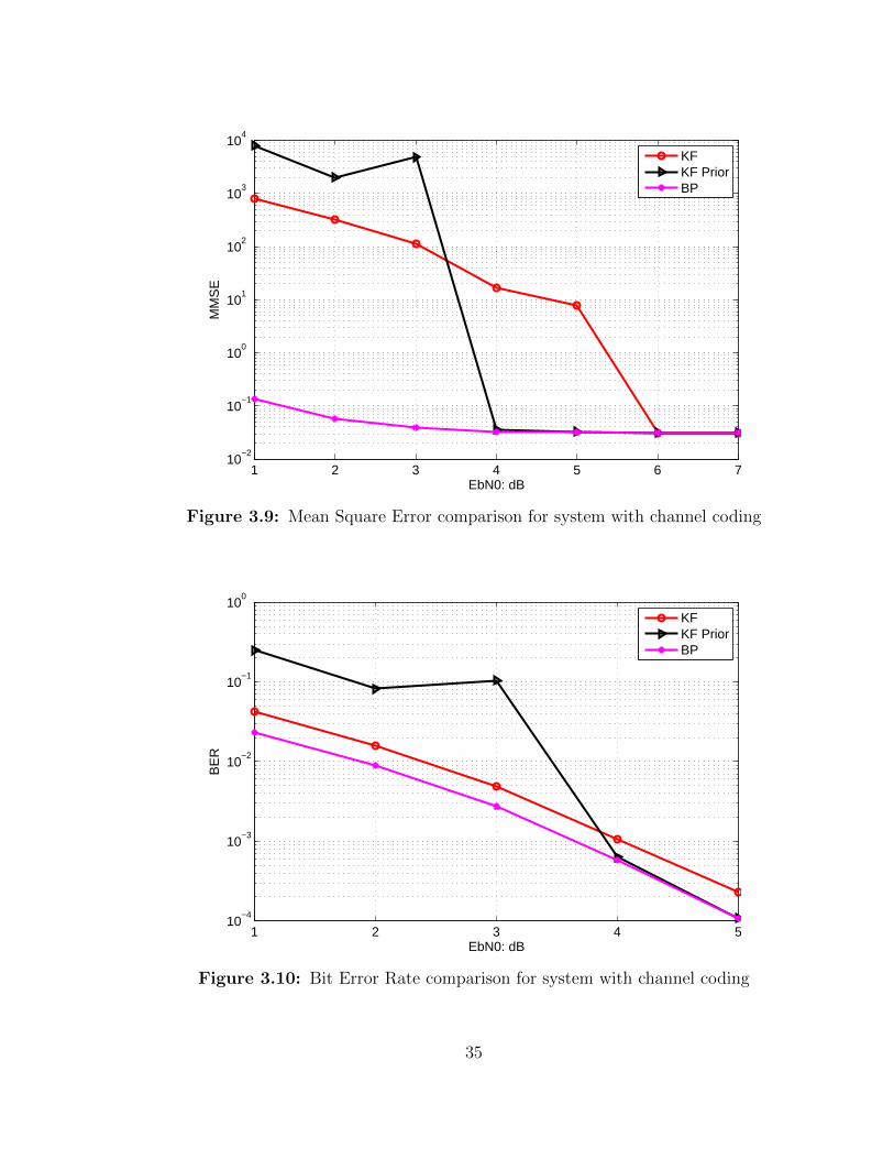
Figures 3.9 and 3.10 show the simulation results for the channel coded case with
different Eb/N0. As shown in the figures, the performance of ’BP’ is always the best.
The performance of system dynamics assisted channel decoding is also seen in ’KF
prior’ when Eb/N0 is equal to 4dB and 5dB. However, there is error propagation for
’KF prior’ when Eb/N0 is lower than 4dB. The cause is similar as that for uncoded
case.
3.6 Conclusions
In this chapter, we have proposed to use Kalman Filter based and Pearl’s BP
based decoding procedure (including the demodulation procedure) to exploit the
redundancy, i.e., the nature encoding in the system state for the system with no or
weak channel coding protection in the context of WNCS. The numerical simulation
results have shown that, for coded case there is performance gain from system
dynamics assisted channel decoding. In addition, for estimator keeping erroneous
34
1 2 3 4 5 6 710
−2
10−1
100
101
102
103
104
EbN0: dB
MM
SE
KFKF PriorBP
Figure 3.9: Mean Square Error comparison for system with channel coding
1 2 3 4 510
−4
10−3
10−2
10−1
100
EbN0: dB
BE
R
KFKF PriorBP
Figure 3.10: Bit Error Rate comparison for system with channel coding
35

packets the performance can be improved by transferring the statistics of the estimate
of system observation to estimator.
36
Chapter 4
Quickest Detection Based Error
Propagation Detection and Its
Application for the Protection of
System Dynamics Assisted
Channel Decoding
4.1 Introduction
Because of low installation and reconfiguration cost wireless communication has been
widely applied in networked control system (NCS). NCS is a control system which
uses multi-purpose shared network as communication medium to connect spatially
distributed components of control system including sensors, actuator, controller.
The integration of wireless communication in NCS is challenging due to channel
unreliability such as fading, shadowing, interference, mobility and receiver thermal
noise leading to packet corruption, packet dropout and packet transmission delay.
37
In chapter 3 we proposed to utilize time-domain redundancy of system dynamics
to assist channel decoding and designed a belief propagation (BP) based channel
decoding and state estimation algorithm. The effectiveness of this proposed channel
decoding and state estimation algorithm is verified by numerical results. However, in
chapter 3, the simulation results especially Kalman Filtering based herustic approach
show error propagation at low SNR. Note that the error propagation for BP based
channel decoding and state estimation is also observed in our conference paper with
different initial simulation condition (Gong et al., 2011). In order to guarantee the
reliability of NCS, it is necessary to detect and eliminate error propagation from
decoding procedure. In this chapter, at first we show the root cause for error
propagation. Then, quickest detection based algorithm is proposed to detect error
propagation. We also apply this proposed error propagation detection algorithm into
system dynamics assisted channel decoding and state estimation algorithm. The
error porpagation detection algorithm is running at the same time with the system
dynamics assisted channel decoding and state estimation. Once propagation of errors
is detected, then system dynamics assisted channel decoding and state estimation
module is reset to eliminate propagation error.
The organization of this chapter is as follows. In section 4.2 the system model,
communication model and BP based channel decoding and state estimation algorithm
are briefly introduced. Section 4.3 analyzes the root cause for error propagation.
Then, quickest detection based error propagation detection algorithm is proposed in
section 4.4. Section 4.5 shows how to integrate quickest detection based propagation
error detection algorithm into the framework of system dynamics assisted channel
decoding and state estimation. The simulation results are demonstrated in section
4.6. Section 4.7 concludes the work in this chapter.
38
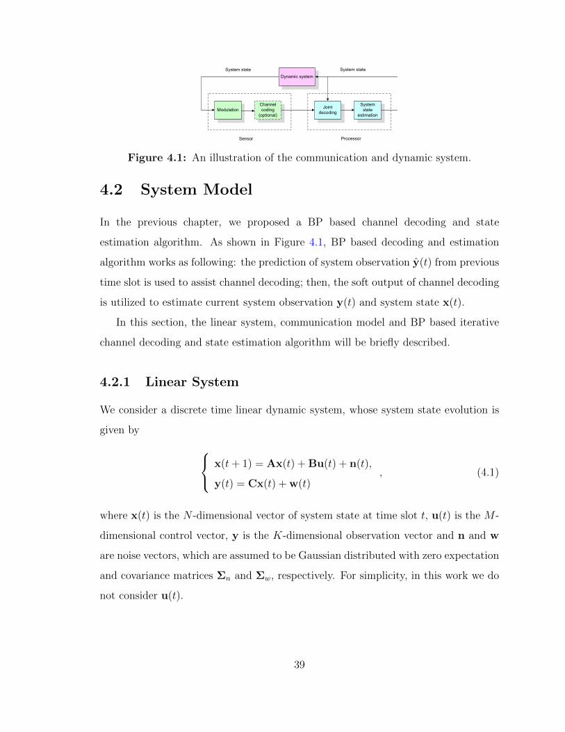
Modulation
Channel
coding
(optional)
Joint
decoding
System
state
estimation
Dynamic system
Sensor Processor
System stateSystem state
Figure 4.1: An illustration of the communication and dynamic system.
4.2 System Model
In the previous chapter, we proposed a BP based channel decoding and state
estimation algorithm. As shown in Figure 4.1, BP based decoding and estimation
algorithm works as following: the prediction of system observation y(t) from previous
time slot is used to assist channel decoding; then, the soft output of channel decoding
is utilized to estimate current system observation y(t) and system state x(t).
In this section, the linear system, communication model and BP based iterative
channel decoding and state estimation algorithm will be briefly described.
4.2.1 Linear System
We consider a discrete time linear dynamic system, whose system state evolution is
given by x(t+ 1) = Ax(t) + Bu(t) + n(t),
y(t) = Cx(t) + w(t), (4.1)
where x(t) is the N -dimensional vector of system state at time slot t, u(t) is the M -
dimensional control vector, y is the K-dimensional observation vector and n and w
are noise vectors, which are assumed to be Gaussian distributed with zero expectation
and covariance matrices Σn and Σw, respectively. For simplicity, in this work we do
not consider u(t).
39
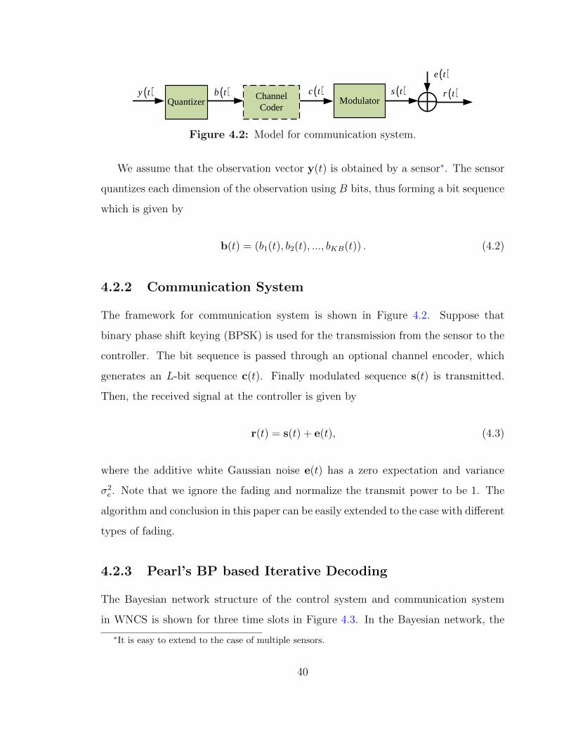
QuantizerChannel Coder
( )y t ( )b t
( )e t
( )r t( )c tModulator
( )s t
Figure 4.2: Model for communication system.
We assume that the observation vector y(t) is obtained by a sensor∗. The sensor
quantizes each dimension of the observation using B bits, thus forming a bit sequence
which is given by
b(t) = (b1(t), b2(t), ..., bKB(t)) . (4.2)
4.2.2 Communication System
The framework for communication system is shown in Figure 4.2. Suppose that
binary phase shift keying (BPSK) is used for the transmission from the sensor to the
controller. The bit sequence is passed through an optional channel encoder, which
generates an L-bit sequence c(t). Finally modulated sequence s(t) is transmitted.
Then, the received signal at the controller is given by
r(t) = s(t) + e(t), (4.3)
where the additive white Gaussian noise e(t) has a zero expectation and variance
σ2e . Note that we ignore the fading and normalize the transmit power to be 1. The
algorithm and conclusion in this paper can be easily extended to the case with different
types of fading.
4.2.3 Pearl’s BP based Iterative Decoding
The Bayesian network structure of the control system and communication system
in WNCS is shown for three time slots in Figure 4.3. In the Bayesian network, the
∗It is easy to extend to the case of multiple sensors.
40
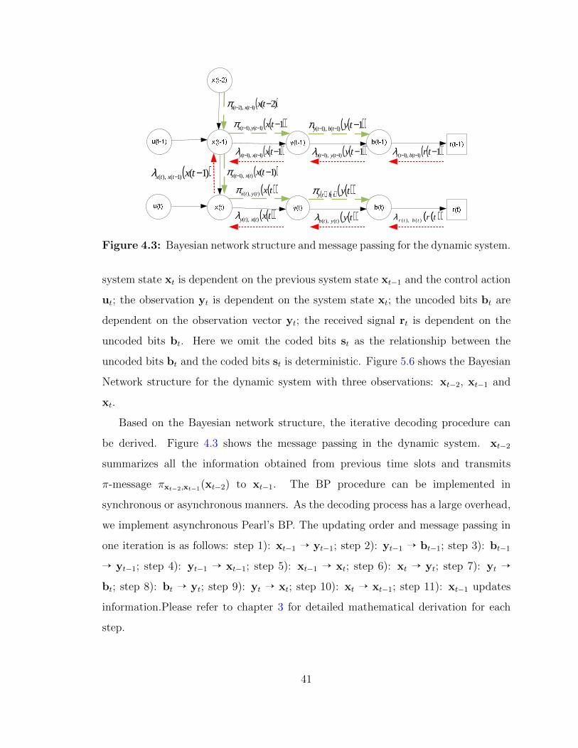
( )( )1)1(),1( −−− txtytxπ ( )( )1)1(),1( −−− tytbtyπ
( )( )1)1(),1( −−− tytytbλ( )( )1)1(),1( −−− txtxtyλ
( ))2()1(),2( −−− txtxtxπ
( )( )1)1(),1( −−− trtbtrλ
( )( )txtytx )(),(π ( ) ( ) ( )( )tytbty ,π
( )( )tytytb )(),(λ( )( )txtxty )(),(λ
( ))1()(),1( −− txtxtxπ
( )( )trtbtr )(),(λ
( ))1()1(),( −− txtxtxλ
Figure 4.3: Bayesian network structure and message passing for the dynamic system.
system state xt is dependent on the previous system state xt−1 and the control action
ut; the observation yt is dependent on the system state xt; the uncoded bits bt are
dependent on the observation vector yt; the received signal rt is dependent on the
uncoded bits bt. Here we omit the coded bits st as the relationship between the
uncoded bits bt and the coded bits st is deterministic. Figure 5.6 shows the Bayesian
Network structure for the dynamic system with three observations: xt−2, xt−1 and
xt.
Based on the Bayesian network structure, the iterative decoding procedure can
be derived. Figure 4.3 shows the message passing in the dynamic system. xt−2
summarizes all the information obtained from previous time slots and transmits
π-message πxt−2,xt−1(xt−2) to xt−1. The BP procedure can be implemented in
synchronous or asynchronous manners. As the decoding process has a large overhead,
we implement asynchronous Pearl’s BP. The updating order and message passing in
one iteration is as follows: step 1): xt−1 Õ yt−1; step 2): yt−1 Õ bt−1; step 3): bt−1
Õ yt−1; step 4): yt−1 Õ xt−1; step 5): xt−1 Õ xt; step 6): xt Õ yt; step 7): yt Õ
bt; step 8): bt Õ yt; step 9): yt Õ xt; step 10): xt Õ xt−1; step 11): xt−1 updates
information.Please refer to chapter 3 for detailed mathematical derivation for each
step.
41
4.3 Cause For Error Propagation
As observed in the simulation results of system dynamics based channel decoding and
state estimation algorithm, there exists error propagation at low SNR. In this section
we will use a simplified example to illustrate the cause of error propagation, which is
estimation error of MSE of system observation prediction. In this section we assume
that system observation y(t) has just one dimension and the distribution of y(t) is
standard Gaussian.
In previous chapter, in BP based channel decoding and state estimation algorithm,
message πyt,bt(yt) is passed from yt to bt to assist channel decoding. In other words,
πyt,bt(yt) and received signals r(t) are used to jointly estimate yt. However, the
distribution of πyt,bt(yt) is assumed to be Gaussian with mean yπ,t and covariance
matrix Sπ,t. The Gaussian assumption does not hold all the time; in addition, yπ,t
and Sπ,t are estimated value. We evaluate the impact of error of estimated Sπ,t on the
estimation of system state and observation. Since there is no analytical expression for
the conversion of πyt,bt(yt) to the priori information of b(t), the evaluation is done in
continous domain.
Figure 4.4 shows the ideal model for joint estimation. rsc(t) is the estimated y(t)
based received signals r(t), and rsp(t) is the predicted y(t) based on πyt,bt(yt). The
detailed procedure to estimate rsc(t) from received signals r(t) will be provided in the
next section. In this section, we model rsc(t) as
rsc(t) = y(t) + σcNc(t) (4.4)
in which σ2c is the MSE of rsc(t) and Nc(t) is standard Gaussian noise. The prediction
of y(t), i.e, rsp(t), based on πyt,bt(yt) is modeled as
rsp(t) = y(t) + σpNp(t) (4.5)
in which σ2p is the MSE of rsp(t) and Np(t) is standard Gaussian noise.
42

( )y t
( )p pN tδ
( )c cN tδ
( )scr t
( )spr t
Figure 4.4: Model for estimation from received signal and prediction with knownσ2c and σ2
p
( )y t
( )2ˆp e pmse N tδ +
( )c cN tδ
( )scr t
( )spr t
Figure 4.5: Model for estimation from received signal from channel and predictionwith known σ2
c and estimated σ2p
Then the ideal joint estimation of y(t) is:
y(t) = E[y(t)|rsc(t), rsp(t), σ2c , σ
2p]
=
1σ2c
1 + 1σ2c
+ 1σ2p
rsc(t) +
1σ2p
1 + 1σ2c
+ 1σ2p
rsp(t) (4.6)
mse(y(t)) = E[(y(t)− yt)2] =1
1 + 1σ2c
+ 1σ2p
(4.7)
43
In the above ideal model, we assume that σp and σc are known. However, σp and
σc are estimated values. When channel noise power σ2e is known, then the estimation
of σc is correct. But σp depends on estimation over all previous time slots. It is more
likely that σp deviates from its real value. Therefore, there exists error for estimation
of σ2p. We model the estimation error as msee:
msee = σ2p − σ2
p (4.8)
As both σ2p and σ2
p are positive values. The range for msee is [σ2p,+∞]. Figure
4.5 shows the model of observation with estimation error. The joint estimation is:
ye(t) = E[y(t)|rsc(t), rsp(t), σ2c , σ
2p]
=
1σ2c
1 + 1σ2c
+ 1σ2p
rsc(t) +
1σ2p
1 + 1σ2c
+ 1σ2p
rsp(t) (4.9)
and MSE is:
msee(y(t)) =1
1 + 1σ2c
+ 1σ2p
+
mseeσ4p(
1 + 1σ2c
+ 1σ2p
)2 (4.10)
Besides joint estimation, we can also estimate y(t) based on received channel
signal:
yc(t) =
1σ2c
1 + 1σ2c
rsc(t) (4.11)
and MSE is:
msec(y(t)) =1
1 + 1σ2c
(4.12)
As shown in Figure 4.6, when msee is small, joint estimation is better than
estimation only from channel observation. However, when msee becomes larger, then
44
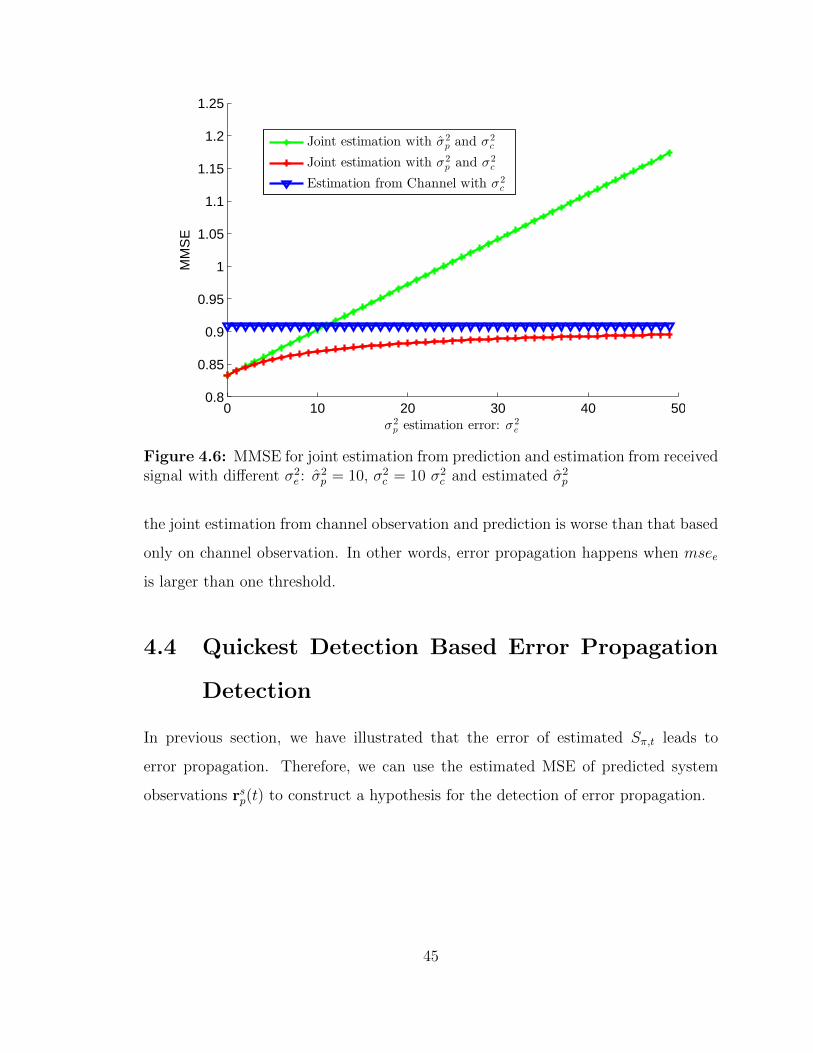
0 10 20 30 40 500.8
0.85
0.9
0.95
1
1.05
1.1
1.15
1.2
1.25
σ2pestimation error: σ2
e
MM
SE
Joint estimation with σ2pand σ
2c
Joint estimation with σ2pand σ
2c
Estimation from Channel with σ2c
Figure 4.6: MMSE for joint estimation from prediction and estimation from receivedsignal with different σ2
e : σ2p = 10, σ2
c = 10 σ2c and estimated σ2
p
the joint estimation from channel observation and prediction is worse than that based
only on channel observation. In other words, error propagation happens when msee
is larger than one threshold.
4.4 Quickest Detection Based Error Propagation
Detection
In previous section, we have illustrated that the error of estimated Sπ,t leads to
error propagation. Therefore, we can use the estimated MSE of predicted system
observations rsp(t) to construct a hypothesis for the detection of error propagation.
45
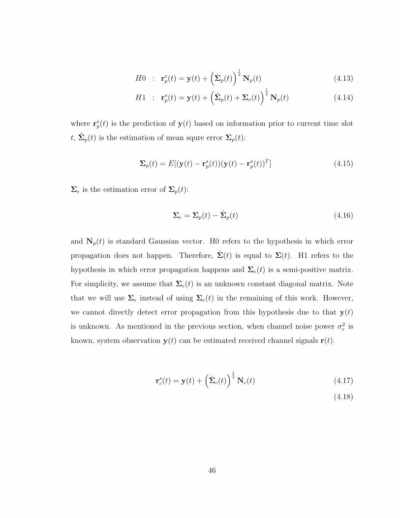
H0 : rsp(t) = y(t) +(Σp(t)
) 12Np(t) (4.13)
H1 : rsp(t) = y(t) +(Σp(t) + Σe(t)
) 12Np(t) (4.14)
where rsp(t) is the prediction of y(t) based on information prior to current time slot
t, Σp(t) is the estimation of mean squre error Σp(t):
Σp(t) = E[(y(t)− rsp(t))(y(t)− rsp(t))T ] (4.15)
Σe is the estimation error of Σp(t):
Σe = Σp(t)− Σp(t) (4.16)
and Np(t) is standard Gaussian vector. H0 refers to the hypothesis in which error
propagation does not happen. Therefore, Σ(t) is equal to Σ(t). H1 refers to the
hypothesis in which error propagation happens and Σe(t) is a semi-positive matrix.
For simplicity, we assume that Σe(t) is an unknown constant diagonal matrix. Note
that we will use Σe instead of using Σe(t) in the remaining of this work. However,
we cannot directly detect error propagation from this hypothesis due to that y(t)
is unknown. As mentioned in the previous section, when channel noise power σ2e is
known, system observation y(t) can be estimated received channel signals r(t).
rsc(t) = y(t) +(Σc(t)
) 12Nc(t) (4.17)
(4.18)
46
where rsc(t) is the estimation of y(t) from channel observation and the kth element of
rsc(t) is:
rsc,k(t) =i=B−1∑i=0
skB+i(t)QiI , k = 0, · · · , K − 1 (4.19)
where bkB+i(t) is the estimation of ith modulated bit of quantized yk(t), skB+i(t),
based on channel observation rkB+i(t) and is equal to:
skB+i(t) = P (SkB+i(t) = 1|rkB+i(t))− P (skB+1(t) = −1|rkB+i(t))
= tan
(rkB+i(t)
(σbc)2
)(4.20)
and QI is the base of quantization and B is the number of quantization bits. Σc(t) is
the MSE of estimated y(t) from channel observation, which is a diagonal matrix and
the kth diagonal element of Σc(t) is:
Σc,k(t) =i=B−1∑i=0
msekB+i(t)Q2iI (4.21)
where msekB+i(t) is the mse of the estimated skB+i(t) from channel only:
msekB+i(t) = E[(bkB+i(t)− bkB+i(t))2] = 1− tan2
(rkB+i(t)
(σbc)2
)(4.22)
Then, we use rsc(t) as reference for the above hypothesis detection. Note that
the way to obtain rsc(t) works for uncoded systrem and the system systematic coding
case. For coding case, if the coding scheme is not systematic, then more complicated
procedures are needed to obtain estimated rsc(t).
Deduct rsc(t) from rsp(t), then the hypothesis is:
H0 : d(t) =(Σp(t)
) 12Np(t)−
(Σc(t)
) 12Nc(t)
H1 : d(t) =(Σp(t) + Σe
) 12Np(t)−
(Σc(t)
) 12Nc(t) (4.23)
47

where
d(t) = rsp(t)− rsc(t) (4.24)
We re-write above hypothesis equation as:
H0 : d(t) = (Σ0(t))12 N0(t)
H1 : d(t) = (Σ0(t) + Σe)12 N1(t) (4.25)
where
Σ0(t) = Σp(t) + Σc(t) (4.26)
N0(t) and N1(t) are K-dimension standard Gaussian variables. From the above
equations, when error propagation happens at the unknown time instant t0, the
distribution of d(t) is changed from Σ0(t) to Σ0(t) + Σe, where Σe is unknown. In
this paper, we adopt CUSUM algorithm to estimate unknown parameters t0 and Σe.
Based on CUSUM method we construct the log-likelihood ratio for the observations
d(t) from time j up to k, which is equal to:
Skj (Σe) =k∑t=j
lθ(t) =k∑t=1
PΣ0(t)(d(t))
PΣ0(t)+Σe(d(t))(4.27)
where:
PΣ0(t)(d(t)) =1
(2π|Σ0(t)|)K2dT (t)Σ−1
0 (t)dT (t) (4.28)
and
PΣ0(t)+Σe(d(t)) =1
(2π|Σ0(t) + Σe|)K2
dT (t)(Σ0(t) + Σe)−1dT (t) (4.29)
48

The statistical metric is the maximum likelihood estimation of Σe, which results
in the decision function given by
gk = max1≤j≤k
supΣe∈Θ
Skj (Σe) (4.30)
where Θ is the region of Σe. Then the decision rule is H0 is selected; if gk < h
H1 is selected; if gk ≥ h(4.31)
where h is the pre-determined threshold. The alarm time for error propagation is
obtained by the following stopping rule:
t0 = min{k : gk ≥ h} (4.32)
Finally, the procedure of CUSUM quickest detection based error propagation
detection algorithm is shown in Procedure 1.
Procedure 1 Procedure for CUSUM quickest detection based propagation errordetection algorithm
1: for each time slot t, t = 1, 2, ..., do2: Current observation prediction rsp(t) and Σp(t) are obtained from time slot t−1;
3: Estimation from channel received signals rsc(t) and Σc(t) are obtained viaequation 4.17;
4: Obtain d(t) via equation 4.24 ;5: Calculate detection metric gk from equation 4.30;6: Make decision based on rule defined in equation 4.31 ;7: if Propagaton error is deteced then8: calculate time slot of error propagation t0(t) from equation 4.32.9: end if
10: end for
49

( )p trQuickest detection
for error propagation
( )qe t
Channel Decoder/State Estimator
Error Propagation Detected?
Yes
Reset( )tr
Figure 4.7: BP based channel decoding and system estimation with protection oferror propagation detection
4.5 System Dynamics Assisted Channel Decoding
and State Estimation with Protection of Error
Propagation Detection
In this section, we demonstrate how to utilize the proposed error propagation
dedection algorithm to improve performance and robustness of the system dynamics
assisted channel decoding and state estimation algorithm. In this scheme, the channel
decoding and state estimation module resets and discards any priori information from
previous time slots once error propagation is detected. . The framework is shown in
Figure 4.7. The received signal r(t) is input for both modules. rp(t) is sent from BP
based channel decoding and state estimation module to error propagation detection
module. Once error propagation module detects error propagation, it sends a reset
signal to BP based channel decoding and state estimation module. Then, BP based
channel decoding and state estimation module resets the memory and clear up the
error.
4.6 Numerical Simulations
We run the simulations using Matlab to verify the performance of Kalman Filter
based heuristic approach and BP based channel decoding and system estimation with
protection of error propagation detection. The baseline approach is the separated
50
Kalman filtering and decoding process. In the following, these three algorithms are
referred as ‘KF Prior’, ‘BP’ and ‘KF’, respectively. And the corresponding algorithms
with protection of error propagation detection are referred as ‘EP based KF Prior’
and ‘EP based BP’, respectively. The performance metrics are the mean square error
(MSE) of each sample and the average bit error rate (BER). Each simulation runs
1000 times slots. The configuration for simulation is the same as that in section 3.5.
The simulation results for uncoded case and coded case are presented in this section.
4.6.1 Uncoded Case
Figures 4.8 and 4.9 show the simulation results for the uncoded case with different
Eb/N0. The performance of ’EP based BP’ is identical with that of ’BP’. The reason
why we suggest using error propagation detection scheme for ’BP’ is to improve its
robustness. The MSE of ’EP based KF Prior’ is always lower than ’KF’ which means
that error propagation of ’KF prior’ is eliminated by error propagation detection
algorithm. Note that BER of ’EP based KF Prior’ is higher than that of ’KF’ when
Eb/N0 is less than 4dB. At low Eb/N0 the mse gain of ’EP based KF Prior’ over ’KF’
comes from the reset of estimator triggered by error propagation detection scheme
instead of system dynamics assisted channel decoding.
4.6.2 Coded Case
Figures 4.10 and 4.11 show the simulation results for the uncoded case with different
Eb/N0. The results are similar as that for uncoded case. The performance of ’EP
based BP’ is identical with that of ’BP’. The MSE of ’EP based KF Prior’ is always
lower than ’KF’ which means that error propagation of ’KF prior’ is eliminated by
error propagation detection algorithm. Note that BER of ’EP based KF Prior’ is
higher than that of ’KF’ when Eb/N0 is lower than 4dB. At low Eb/N0 the mse gain
of ’EP based KF Prior’ over ’KF’ comes from the reset of estimator triggered by error
propagation detection scheme instead of system dynamics assisted channel decoding.
51
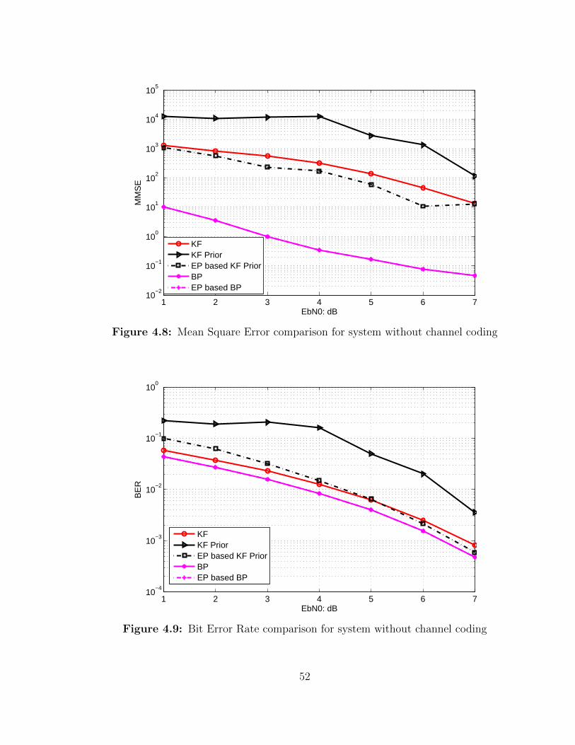
1 2 3 4 5 6 710
−2
10−1
100
101
102
103
104
105
EbN0: dB
MM
SE
KFKF PriorEP based KF PriorBPEP based BP
Figure 4.8: Mean Square Error comparison for system without channel coding
1 2 3 4 5 6 710
−4
10−3
10−2
10−1
100
EbN0: dB
BE
R
KFKF PriorEP based KF PriorBPEP based BP
Figure 4.9: Bit Error Rate comparison for system without channel coding
52
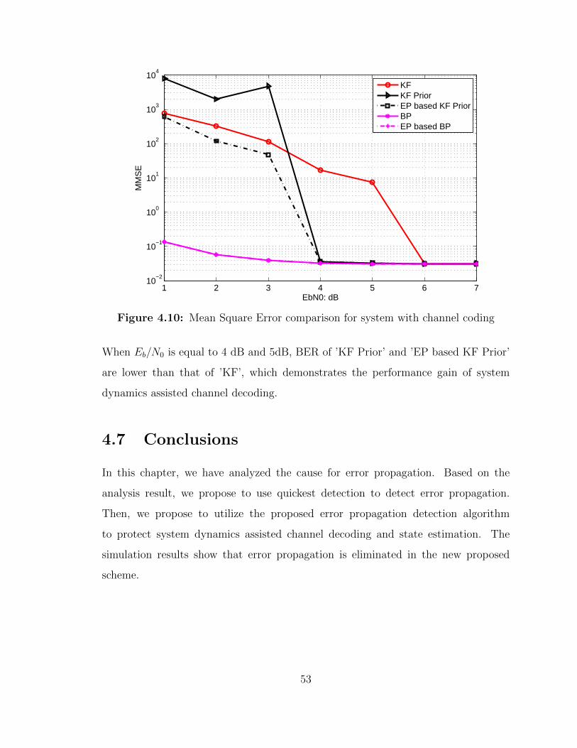
1 2 3 4 5 6 710
−2
10−1
100
101
102
103
104
EbN0: dB
MM
SE
KFKF PriorEP based KF PriorBPEP based BP
Figure 4.10: Mean Square Error comparison for system with channel coding
When Eb/N0 is equal to 4 dB and 5dB, BER of ’KF Prior’ and ’EP based KF Prior’
are lower than that of ’KF’, which demonstrates the performance gain of system
dynamics assisted channel decoding.
4.7 Conclusions
In this chapter, we have analyzed the cause for error propagation. Based on the
analysis result, we propose to use quickest detection to detect error propagation.
Then, we propose to utilize the proposed error propagation detection algorithm
to protect system dynamics assisted channel decoding and state estimation. The
simulation results show that error propagation is eliminated in the new proposed
scheme.
53

1 2 3 4 510
−4
10−3
10−2
10−1
100
EbN0: dB
BE
R
KFKF PriorEP based KF PriorBPEP based BP
Figure 4.11: Bit Error Rate comparison for system with channel coding
54

Chapter 5
MSE-based Transfer Chart for
Performance Evaluation of Belief
Propagation based Sequential and
Iterative Channel Decoding and
System Estimation
5.1 Introduction
Because of low installation and reconfiguration cost wireless communication has been
widely applied in networked control system (NCS). NCS is a control system which
uses multi-purpose shared network as communication medium to connect spatially
distributed components of control system including sensors, actuator, and controller.
The integration of wireless communication in NCS is challenging due to channel
unreliability such as fading, shadowing, interference, mobility and receiver thermal
noise leading to packet corruption, packet dropout and packet transmission delay.
55
In chapter 3 we proposed to utilize time-domain redundancy of system state
to assist channel decoding and designed a belief propagation (BP) based channel
decoding and system state estimation algorithm. And the effectiveness of this
proposed iterative channel decoding and system state estimation algorithm is verified
by numerical results. In this chapter, we evaluate its performance from the following
perspectives:
• How much gain can be obtained from using redundancy of system state in
time-domain to assist channel decoding?
• Does iterative channel decoding and system state estimation converge and help
improve the performance of channel decoding and system state estimation?
• Does the channel decoding and system state estimation converge over time?
As pointed out in chapter 1 NCS is a hybrid system: non-binary and continuous
system state x(t)/observation y(t) and quantized information bits b(t) transmitted in
wireless communication system. In the iterative channel decoding and system state
estimation framework, the priori information transmitted from state estimator to
channel decoder is the prediction of y(t); however, channel decoding requires the
prior information of each quantized bit of y(t). The output of channel decoder
is the extrinsic information of each quantized bit; however, the state estimator
requires estimates of y(t) from channel decoder. The challenge for performance
analysis is how to handle the information exchange between channel decoder which
processes information of quantized bits and state estimator which handles information
of continuous variables. We proposed to use MSE-based chart to analyze the
performance of BP based channel decoding and system state estimation. The
information transferred from non-binary source to channel decoding is the priori
mutual information of transmitted information bits. We used the MSE-based analysis
framework proposed in (Bhattad and Narayanan, 2007) to evaluate the performance
of channel decoding. Then the MSE of decoded information bits is converted to MSE
of system observation estimation.
56
We proposed two models to evaluate the performance of BP based iterative channel
decoding and system state estimation. The first model can be used to check the
following points:
1. Does the iterative channel decoding and estimation converge?
2. How many iterations are sufficient?
3. How much gain can be obtained from redundancy of source?
The second model can be used to evaluate the performance of system state estimation
over time.
The remainder of this chapter is organized as following. Next section, section 5.2
surveys the literature of iterative decoding performance analysis method. Section 5.3
briefly introduce about EXIT and MSE transfer chart for the performance evaluation
of iterative channel decoding. Section 5.4 describes the message passing models
for analysis. Section 5.5 presents the message transfer framework between system
observation and channel decoder. Section 5.6 describes the MSE-base transfer chart,
and section 5.7 presents how to use the MSE-based transfer chart to evaluate BP
based sequential and iterative channel decoding and state estimation. Section 5.8
concludes this chapter.
5.2 Literature Review
In the area of wireless communication, the purpose of performance analysis for
iterative decoding scheme is to find out that, for a given codec and decoder and a given
channel noise power, the message-passing iterative decoder can correct the errors or
not. Then the results of performance analysis can be used to assist the design of codec
and decoder. Gallager (1963) proposed to use density evolution to track the iterative
decoding performance. It is based on the assumption that, for very long codes,
the extrinsic log likelihood ratios (LLRs) passed between the component decoders are
57
independent and identically distributed. Then, for the iterative decoding performance
it is equivalent to track the evolution of extrinsic LLRs probability density function
(pdf) through iterative decoding process. The probability of decoding error tends to
zero if extrinsic LLRs goes to either +∞ or −∞.
ten Brink (1999, 2000, 2001) proposed to use extrinsic information transfer chart
(EXIT) to track the iterative decoding performance. Based on the assumption that
the distribution of extrinsic LLR is Gaussian EXIT tracks mutual information of
extrinsic LLRs instead of pdf. Comparing with density evolution, the computation
for EXIT is simplified. In addition, the evolution of mutual information through
iterative decoding process can be illustrated in a graph and easy to visualize. EXIT
has two properties. One property is about the necessary condition for the convergence
of iterative decoding: the flipped EXIT curve of the outer decoder should lie below the
EXIT curve of the inner coder. The other property is that the area under EXIT curve
of outer code relates to the rate of inner coder. Ashikhmin et al. (2004) demonstrated
that if the a priori channel is an erasure channel, for any outer code of rate R, the
area under the EXIT curve is 1−R. To the best knowledge of us, the area property
of EXIT has been proved only for erasure priori channel.
Another alternative for density evolution is MSE chart. Instead of tracking mutual
information MSE is proposed to track the iterative decoding performance (Bhattad
and Narayanan, 2007). The MSE chart analysis method is based on the relationship
between mutual information and minimum mean square error (MMSE) in AWGN
channel (Guo et al., 2005). Bhattad and Narayanan (2007) has proven the area
property of MSE chart when the priori channel is Gaussian.
In this chapter, we also used MSE chart to analyze the performance of iterative
channel decoding and state estimation. Comparing with (Guo et al., 2005) the
difference in this dissertation work is that we have a hybrid model. The system state
and observation are non-binary source in continuous domain; on the other hand the
information transmitted in wireless system is quantized bits. Therefore, the method
proposed in (Guo et al., 2005) cannot be used directly. The challenge is how to
58
handle the message transfer between non-binary source and information bits. The
other difference is that the source is correlated over time. The estimation error from
previous time slots also affects the performance of estimation in current time slot.
Therefore, besides evaluating the performance of iterative channel decoding and state
estimation in two time slots, it is also very important to evaluate the performance of
state estimation over time.
Another area in wireless communication related to our work is joint source and
channel decoding (Yin et al., 2002; Mei and Wu, 2006; Pan et al., 2006; Pu et al.,
2007; Ramzan et al., 2007; Garcia-Frias and Villasenor, 1997, 1998, 2001; Garcia-Frias
and Zhao, 2001, 2002; Garcia-Frias and Zhong, 2003; Garcia-Frias et al., 2003). The
idea of joint source and channel decoding is to utilize redundancy in source to assist
channel decoding. Our work can also be considered as one special case of joint source
and channel decoding. However, there are two major differences. One difference is
that most works focus on binary source and EXIT chart was used for performance
analysis (Fresia et al., 2010). Zhao and Garcia-Frias (2002, 2005) considered the case
with non-binary source, but the performance analysis was not provided. The other
difference is these works considered the joint source and channel decoding over only
two time slots. In our work, the dynamic state changes over time. Therefore, the
performance of channel decoding and system estimation at the current time slots also
impacts its performance in the future. Therefore, we also study the performance of
iterative estimation and decoding over time.
In NCS area studying the impact of the communication on estimation and
control has received considerable attentions. The impact of quantization on stability
of estimation and control system has been studied extensively (Nair and Evans,
2004),(Tatikonda and Mitter, 2004),(Cover and Thomas, 1991), (Minero et al., 2009),
(You and Xie, 2011) and (Minero et al., 2013). However, the analysis in these works
is based on the assumption that the transmission over networking is loss-less. Most
works considering the impact of communication on estimation and control generally
assume that all erroneous packets are dropped by the estimator. Therefore, these
59

works studies only the impact of packet drop or packet delay on the stability and
performance of estimation and control (Sinopoli et al., 2004), (Imer et al., 2006),
(Schenato et al., 2007), (Schenato, 2008). It was proposed by Mostofi and Murray
(2009c) keep some erroneous packets can improve stability and performance for real-
time control application.Mostofi and Murray (2009c). Mostofi and Murray (2009b)
considered the communication noise resulted from accepting corrupted received
samples and reformulated the Kalman filter based estimation problem. The criteria
to keep or drop erroneous packets were set in this work. However, it is based on
the assumption that the knowledge about the statistics of communication noise is
available. Although the statistics of communication noise for uncoded case was
computed by Mostofi and Murray (2004), it is difficult to compute the statistics of
communication noise for coded case. In our work, we considered the case in which all
erroneous packets are accepted, which is reasonable as we can estimate the statistics
of communication noise. Since we utilize the redundancy of system state over time
and use the estimates from previous time slot to assist channel decoding at the current
time slot, the statistics of communication noise not only depends on wireless channel
but also on the estimate from previous time slot. In our work, we also estimate the
statistics of communication noise online.
5.3 Preliminaries: EXIT Chart and MSE Chart
for Iterative Decoding of Serially Concate-
nated Coding Scheme
In this section, we review the concept of EXIT-chart and MSE-chart by the iterative
decoding of a serially concatenated coding scheme. In subsection 5.3.1 we use
an example to demonstrate serially concatenated coding scheme and its iterative
decoding process. Then, in subsection 5.3.2 we review about how to use EXIT chart
and MSE chart to analyze the performance of iterative decoding.
60
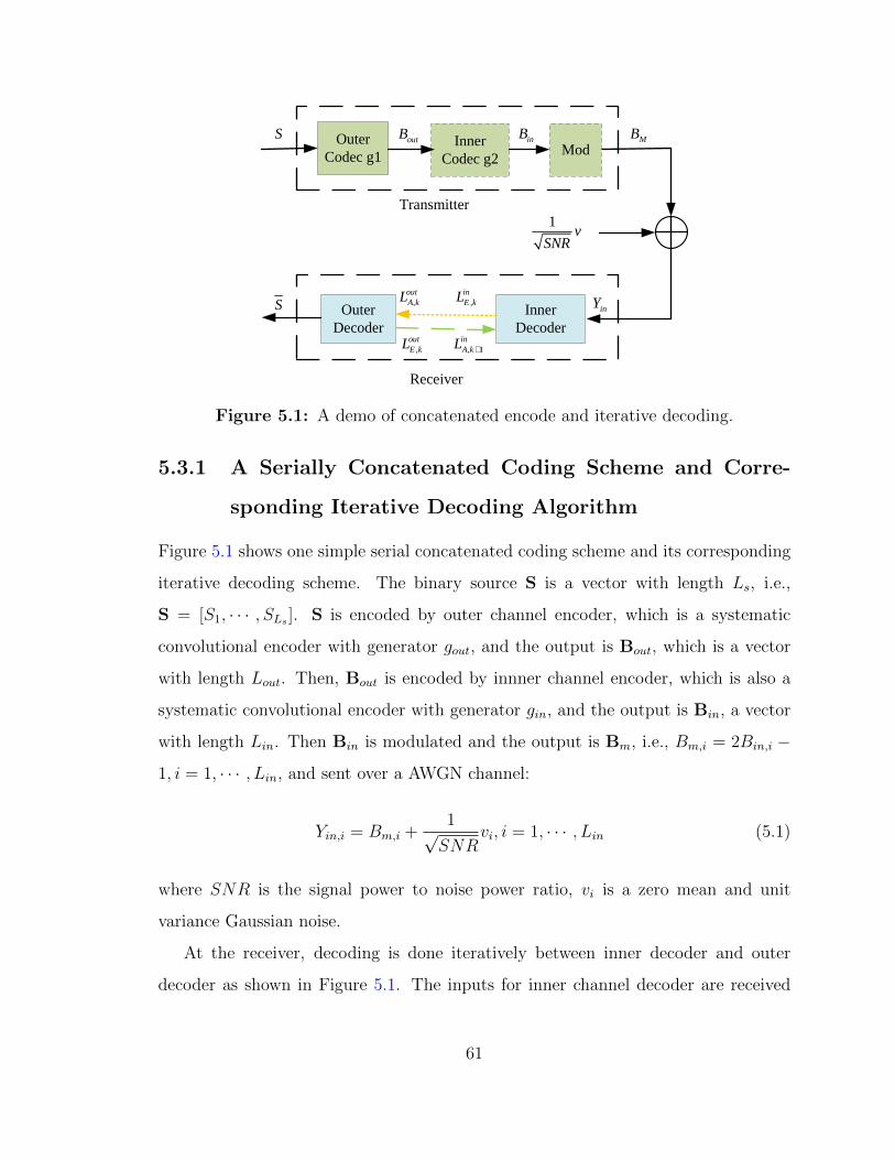
Outer Codec g1
Inner Codec g2
Transmitter
Inner Decoder
Outer Decoder
Receiver
,inE kL,
outA kL
,outE kL , 1
inA kL +
S outB inB
inYS
Mod
1v
SNR
MB
Figure 5.1: A demo of concatenated encode and iterative decoding.
5.3.1 A Serially Concatenated Coding Scheme and Corre-
sponding Iterative Decoding Algorithm
Figure 5.1 shows one simple serial concatenated coding scheme and its corresponding
iterative decoding scheme. The binary source S is a vector with length Ls, i.e.,
S = [S1, · · · , SLs ]. S is encoded by outer channel encoder, which is a systematic
convolutional encoder with generator gout, and the output is Bout, which is a vector
with length Lout. Then, Bout is encoded by innner channel encoder, which is also a
systematic convolutional encoder with generator gin, and the output is Bin, a vector
with length Lin. Then Bin is modulated and the output is Bm, i.e., Bm,i = 2Bin,i −
1, i = 1, · · · , Lin, and sent over a AWGN channel:
Yin,i = Bm,i +1√SNR
vi, i = 1, · · · , Lin (5.1)
where SNR is the signal power to noise power ratio, vi is a zero mean and unit
variance Gaussian noise.
At the receiver, decoding is done iteratively between inner decoder and outer
decoder as shown in Figure 5.1. The inputs for inner channel decoder are received
61
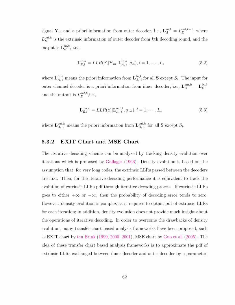
signal Yin and a priori information from outer decoder, i.e., Lin,kA = Lout,k−1
E , where
Lout,kE is the extrinsic information of outer decoder from kth decoding round, and the
output is Lin,kE , i.e.,
Lin,kE,i = LLR(Si|Yin,L
in,kA, i, gin), i = 1, · · · , Ls (5.2)
where Lin,kA, i means the priori information from Lin,k
A, i for all S except Si. The input for
outer channel decoder is a priori information from inner decoder, i.e., Lout,kA = Lin,k
E
and the output is Lout,kE ,i.e.,
Lout,kE,i = LLR(Si|Lout,k
A, i , gout), i = 1, · · · , Ls (5.3)
where Lout,kA, i means the priori information from Lout,k
A, i for all S except Si.
5.3.2 EXIT Chart and MSE Chart
The iterative decoding scheme can be analyzed by tracking density evolution over
iterations which is proposed by Gallager (1963). Density evolution is based on the
assumption that, for very long codes, the extrinsic LLRs passed between the decoders
are i.i.d. Then, for the iterative decoding performance it is equivalent to track the
evolution of extrinsic LLRs pdf through iterative decoding process. If extrinsic LLRs
goes to either +∞ or −∞, then the probability of decoding error tends to zero.
However, density evolution is complex as it requires to obtain pdf of extrinsic LLRs
for each iteration; in addition, density evolution does not provide much insight about
the operations of iterative decoding. In order to overcome the drawbacks of density
evolution, many transfer chart based analysis frameworks have been proposed, such
as EXIT chart by ten Brink (1999, 2000, 2001), MSE chart by Guo et al. (2005). The
idea of these transfer chart based analysis frameworks is to approximate the pdf of
extrinsic LLRs exchanged between inner decoder and outer decoder by a parameter,
62
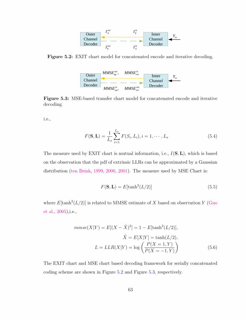
Inner Channel Decoder
Outer Channel Decoder
inAI
outAI in
EI
outEI
inY
Figure 5.2: EXIT chart model for concatenated encode and iterative decoding.
Inner Channel Decoder
Outer Channel Decoder
,in outap extMMSE MMSE
,out inap extMMSE MMSE
inY
Figure 5.3: MSE-based transfer chart model for concatenated encode and iterativedecoding.
i.e.,
F (S,L) =1
Ls
Ls∑i=1
F (Si, Li), i = 1, · · · , Ls (5.4)
The measure used by EXIT chart is mutual information, i.e., I(S,L), which is based
on the observation that the pdf of extrinsic LLRs can be approximated by a Gaussian
distribution (ten Brink, 1999, 2000, 2001). The measure used by MSE Chart is:
F (S,L) = E[tanh2(L/2)] (5.5)
where E[tanh2(L/2)] is related to MMSE estimate of X based on observation Y (Guo
et al., 2005),i.e.,
mmse(X|Y ) = E[(X − X)2] = 1− E[tanh2(L/2)],
X = E[X|Y ] = tanh(L/2),
L = LLR(X|Y ) = log
(P (X = 1, Y )
P (X = −1, Y )
)(5.6)
The EXIT chart and MSE chart based decoding framework for serially concatenated
coding scheme are shown in Figure 5.2 and Figure 5.3, respectively.
63

0 0.1 0.2 0.3 0.4 0.5 0.6 0.7 0.8 0.9 10
0.1
0.2
0.3
0.4
0.5
0.6
0.7
0.8
0.9
1
IinA
, IoutE
Iin E, I
out
A
Inner DecoderOuter Decoder
Figure 5.4: An example of EXIT chart for concatenated encode and iterativedecoding, gout = gin = [1, 1, 0, 1; 1, 0, 0, 1], SNR = −2dB
The transfer chart includes two transfer curves, one curve is the measure for
the priori information of inner decoder, i.e., F inA (S,L), versus the measure for the
extrinsic information of inner decoder, i.e., F inE (S,L); the other curve is the measure
for the extrinsic information of out decoder, i.e., F outE (S,L), versus the measure for
the extrinsic information of inner decoder, i.e., F outA (S,L). The EXIT chart and MSE
chart for serially concatenated coding scheme are shown in Figure 5.4 and Figure
5.5, respectively. The predicted decoding path is also shown in these two figures.
The iterative decoding converges if the transfer curve for inner decoder lies above the
flipped transfer curve of outer decoder.
64

0 0.2 0.4 0.6 0.8 10
0.1
0.2
0.3
0.4
0.5
0.6
0.7
0.8
0.9
1
1−mmseinA
, 1−mmseoutE
1−m
mse
in E, 1
−m
mse
out
A
Innder DecoderOuter Decoder
Figure 5.5: An example of MSE-based transfer chart for concatenated encode anditerative decoding, gout = gin = [1, 1, 0, 1; 1, 0, 0, 1], SNR = −2dB
65

5.4 System Model
5.4.1 Linear System
We consider a discrete time linear dynamic system, whose state evolution is given by x(t+ 1) = Ax(t) + Bu(t) + n(t),
y(t) = Cx(t) + w(t), (5.7)
where x(t) is the N -dimensional vector of system state at time slot t, u(t) is the M -
dimensional control vector, y is the K-dimensional observation vector and n and w
are noise vectors, which are assumed to be Gaussian distributed with zero expectation
and covariance matrices Σn and Σw, respectively. For simplicity, in this proposal we
do not consider u(t).
We assume that the observation vector y(t) is obtained by a sensor∗. The sensor
quantizes each dimension of the observation using B bits, thus forming a bit sequence
which is given by
b(t) = (b1(t), b2(t), ..., bKB(t)) . (5.8)
5.4.2 Communication System
Suppose that binary phase shift keying (BPSK) is used for the transmission from
the sensor to the controller. The bit sequence is passed through an optional channel
encoder, which generates an L-bit sequence s(t).Finally modulated sequence s(t) is
transmitted. Then, the received signal at the controller is given by
r(t) = s(t) + e(t), (5.9)
∗It is easy to extend to the case of multiple sensors.
66
where the additive white Gaussian noise e(t) has a zero expectation and variance
σ2e . Note that we ignore the fading and normalize the transmit power to be 1. The
algorithm and conclusion in this work can be easily extended to the case with different
types of fading.
5.4.3 Pearl’s BP based Iterative Decoding
The Bayesian network structure of the control system and communication system
in WNCS is shown for three time slots in Figure 5.6. In the Bayesian network, the
system state xt is dependent on the previous system state xt−1 and the control action
ut; the observation yt is dependent on the system state xt; the uncoded bits bt are
dependent on the observation vector yt; the received signal rt is dependent on the
uncoded bits bt. Here we omit the coded bits st as the relationship between the
uncoded bits bt and the coded bits st is deterministic. Figure 5.6 shows the Bayesian
Network structure for the dynamic system with three observations: xt−2, xt−1 and
xt.
Based on the Bayesian network structure, the iterative decoding procedure can
be derived. Figure 5.6 shows the message passing in the dynamic system. xt−2
summarizes all the information obtained from previous time slots and transmits
π-message πxt−2,xt−1(xt−2) to xt−1. The BP procedure can be implemented in
synchronous or asynchronous manners. As the decoding process has a large overhead,
we implement asynchronous Pearl’s BP. The updating order and message passing in
one iteration is as follows: step 1): xt−1 Õ yt−1; step 2): yt−1 Õ bt−1; step 3): bt−1
Õ yt−1; step 4): yt−1 Õ xt−1; step 5): xt−1 Õ xt; step 6): xt Õ yt; step 7): yt Õ
bt; step 8): bt Õ yt; step 9): yt Õ xt; step 10): xt Õ xt−1; step 11): xt−1 updates
information. Please refer to chapter 3 for detailed mathematical derivation for each
step.
67
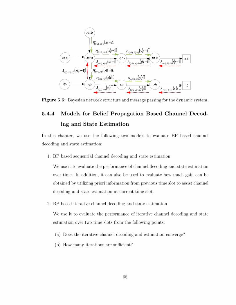
( )( )1)1(),1( −−− txtytxπ ( )( )1)1(),1( −−− tytbtyπ
( )( )1)1(),1( −−− tytytbλ( )( )1)1(),1( −−− txtxtyλ
( ))2()1(),2( −−− txtxtxπ
( )( )1)1(),1( −−− trtbtrλ
( )( )txtytx )(),(π ( ) ( ) ( )( )tytbty ,π
( )( )tytytb )(),(λ( )( )txtxty )(),(λ
( ))1()(),1( −− txtxtxπ
( )( )trtbtr )(),(λ
( ))1()1(),( −− txtxtxλ
Figure 5.6: Bayesian network structure and message passing for the dynamic system.
5.4.4 Models for Belief Propagation Based Channel Decod-
ing and State Estimation
In this chapter, we use the following two models to evaluate BP based channel
decoding and state estimation:
1. BP based sequential channel decoding and state estimation
We use it to evaluate the performance of channel decoding and state estimation
over time. In addition, it can also be used to evaluate how much gain can be
obtained by utilizing priori information from previous time slot to assist channel
decoding and state estimation at current time slot.
2. BP based iterative channel decoding and state estimation
We use it to evaluate the performance of iterative channel decoding and state
estimation over two time slots from the following points:
(a) Does the iterative channel decoding and estimation converge?
(b) How many iterations are sufficient?
68

x(t-1)
x(t) y(t)
x(t+1)
Channel Decoder
( )( 1), ( ) ( 1)x t x t x tπ − −
( )( ), ( 1) ( )x t x t x tπ +
Figure 5.7: Sequential channel decoding and state estimation framework
Model for BP Based Sequential Channel Decoding and State Estimation
We use the framework as shown in Figure 5.7 to evaluate sequential channel decoding
and state estimation over time slots. The priori information from time slot t− 1, i.e.,
πxt−1,x(t)(xt−1), is used to assist channel decoding and state estimation at time slot t.
Note that πx(t−1),x(t)(x(t−1)) is used to model the estimate of x(t−1), and we assume
that it has Guassian distribution with mean xπx,t−1 and covariance matrix Pπx,t−1, i.e.
N (xt−1,xπx,t−1, Pπx,t−1). The first goal is to evaluate how much gain can be obtained
by utilizing πxt−1,x(t)(xt−1) to assist channel decoding and state estimation at time
slot t; the second goal is to evaluate the performance of state estimation over time,
i.e., the evolution of Pπx,t−1 as shown in Figure 5.8.
The message passing in this framework is as below:
1. x(t− 1) Õ x(t), we have
πxt−1,xt(xt−1) = N (xt−1,xπx,t−1, Pπx,t−1), (5.10)
69
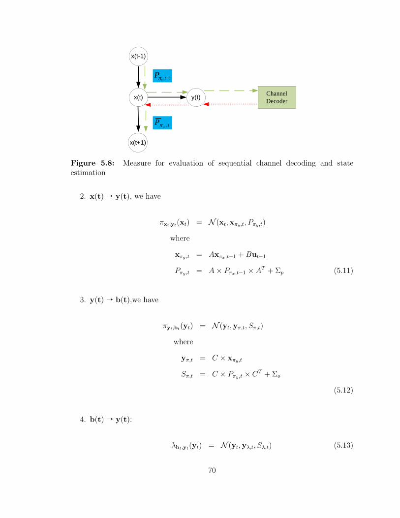
x(t-1)
x(t) y(t)
x(t+1)
Channel Decoder
, 1x tPπ −
,x tPπ
Figure 5.8: Measure for evaluation of sequential channel decoding and stateestimation
2. x(t) Õ y(t), we have
πxt,yt(xt) = N (xt,xπy ,t, Pπy ,t)
where
xπy ,t = Axπx,t−1 +But−1
Pπy ,t = A× Pπx,t−1 × AT + Σp (5.11)
3. y(t) Õ b(t),we have
πyt,bt(yt) = N (yt,yπ,t, Sπ,t)
where
yπ,t = C × xπy ,t
Sπ,t = C × Pπy ,t × CT + Σo
(5.12)
4. b(t) Õ y(t):
λbt,yt(yt) = N (yt,yλ,t, Sλ,t) (5.13)
70

The detailed derivation of yλ,t and Sλ,t is provided in section 5.5.
5. y(t) Õ x(t), we have
λyt,xt(xt) = N (xt,xλy ,t, Pλy ,t)
where
xλy ,t = C−1 × yλ,t,
Pλy ,t = C−1(Sλ,t + Σo)× (C−1)T . (5.14)
6. x(t) Õ x(t + 1): we have
πxt,xt+1(xt) = N (xt,xπx,t, Pπx,t), (5.15)
where the variance is given by
Pπx,t = (P−1l,t + P−1
λ,t )−1, (5.16)
and the expectation is given by
xπx,t = Pπx,t × (P−1l,t × xl,t + P−1
λ,t xλ,t).
where
xl,t = Axπx,t−1 +But−1
Pl,t = A× Pπx,t−1 × AT + Σp (5.17)
Model for BP Based Iterative Channel Decoding and State Estimation
Between Two Time Slots
Figure 5.9 illustrates the model used to evaluate BP based iterative channel decoding
and state estimation between two time slots. The inputs for this model include
71

x(t-1)
x(t) y(t)
x(t+1) y(t+1)
Channel
Decoder
Channel
Decoder
( )( 1), ( ) ( 1)x t x t x tπ − −
Figure 5.9: Model for iterative message passing
x(t-1)
x(t) y(t)
x(t+1) y(t+1)
Channel
Decoder
Channel
Decoder
Observation
Figure 5.10: Model for iterative message passing with known x(t− 1)
received signals in two time slots, i.e., r(t) and r(t + 1) and the priori information
from time slot t− 1, i.e., πx(t−1),x(t)(x(t− 1)).
The goal is to evaluate the performance of iterative channel decoding and state
estimation for different sample of πx(t−1),x(t)(x(t− 1)). Note when πx(t−1),x(t)(x(t− 1))
is equal to 0I, then x(t−1) is a determined state observation. Therefore, this reference
model can be converted to the model shown in Figure 5.10 by setting πx(t−1),x(t)(x(t−
1)) as 0I. If πx(t−1),x(t)(x(t − 1)) is set as +∞I, x(t− 1) is unknown. Then the
reference model is transformed to the model shown in Figure 5.11.
72
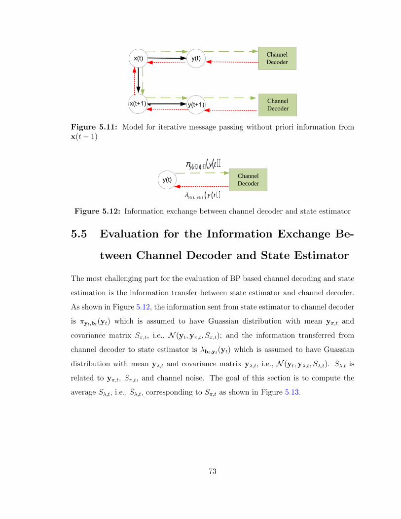
x(t) y(t)
x(t+1) y(t+1)
Channel
Decoder
Channel
Decoder
Figure 5.11: Model for iterative message passing without priori information fromx(t− 1)
y(t)Channel Decoder
( ) ( ) ( )( )tytbty ,π
( )( )( ), ( )b t y t y tλ
Figure 5.12: Information exchange between channel decoder and state estimator
5.5 Evaluation for the Information Exchange Be-
tween Channel Decoder and State Estimator
The most challenging part for the evaluation of BP based channel decoding and state
estimation is the information transfer between state estimator and channel decoder.
As shown in Figure 5.12, the information sent from state estimator to channel decoder
is πyt,bt(yt) which is assumed to have Guassian distribution with mean yπ,t and
covariance matrix Sπ,t, i.e., N (yt,yπ,t, Sπ,t); and the information transferred from
channel decoder to state estimator is λbt,yt(yt) which is assumed to have Guassian
distribution with mean yλ,t and covariance matrix yλ,t, i.e., N (yt,yλ,t, Sλ,t). Sλ,t is
related to yπ,t, Sπ,t, and channel noise. The goal of this section is to compute the
average Sλ,t, i.e., Sλ,t, corresponding to Sπ,t as shown in Figure 5.13.
73

y(t)Channel Decoder
,tSπ
( ), ,t tS Sλ π
Figure 5.13: Measure for information exchange between channel decoder and stateestimator
( )( )( ), ( )b t y t y tλ
Channel Decoder
Quantization
( ), ,,A t tL y Sπ π
( ) ( ) ( )( ), ,, , ,E A t tL L y S e t y tπ π ′ ′
( ) ( ) ( )( )tytbty ,π
( )e t′
( )r t′
( )c t′( )b t′( )y t′
Figure 5.14: Model for Sλ,t based on sample yπ,t, Sπ,t, y′(t) and e′(t)
5.5.1 Quantizing the Information Exchange Between Chan-
nel Decoder and State Estimator
The relationship between Sλ,t and yπ,t, Sπ,t, and channel noise is shown in Figure
5.14.
We assume that the priori information from y(t) to b(t), i.e., πyt,bt(yt), is a
Gaussian vector with mean yπ,t and covariance Sπ,t, i.e.,
πyt,bt(yt) = N (yt,yπ,t,Sπ,t) (5.18)
Note that the physical meaning of πyt,bt(yt) is the prediction of y(t). Then,
πyt,bt(yt) is converted to the priori information of each bit based on quantization
scheme, i.e., LA(yπ,t,Sπ,t). It is a K × B-dimension vector and its ith value is
74
calculated based on quantization scheme:
LA,i(yπ,t,Sπ,t) = logP (bi(t) = 1|y(t) ∈ N (yt,yπ,t,Sπ,t))
P (bi(t) = 0|y(t) ∈ N (yt,yπ,t,Sπ,t))(5.19)
Note that LA,i(yπ,t,Sπ,t) is determined by πyt,bt(yt) and the quantization scheme.
Observation instance y′(t) is sampled from πyt,bt(yt). Then, y′(t) is quantized,
modulated and transmitted over wireless channel. Denote the corresponding
quantized vector, modulated vector, channel noise vector and received vector as b′(t),
S′(t), e′(t), r′(t), respectively.
The inputs for channel decoder is LA(yπ,t,Sπ,t) and r′(t). The information
fedback from channel decoder to state estimator is extrinsic LLR, which is denoted
as L′E (LA(yπ,t,Sπ,t),y′(t), e′(t)). It is a K × B-dimension vector and its ith value is
equal to:
L′E,i (LA(yπ,t,Sπ,t),y′(t), e′(t)) = log
P (bi(t) = 1|LA,i(yπ,t,Sπ,t), r′(t))
P (bi(t) = 0|LA,i(yπ,t,Sπ,t), r′(t))(5.20)
Note that L′E (LA(yπ,t,Sπ,t),y′(t), e′(t)) depends on LA(yπ,t,Sπ,t), y′(t) and e′(t).
Based on L′E (LA(yπ,t,Sπ,t),y′(t), e′(t)), b′(t) can be estimated as (Bhattad and
Narayanan, 2007):
bi(t) =1
2tanh
(1
2L′E,i (LA(yπ,t,Sπ,t),y
′(t), e′(t))
)+
1
2(5.21)
and MMSE in estimating b′i(t) from L′E,i (LA(yπ,t,Sπ,t),y′(t), e′(t)) is given by
mmse (bi(t)|LA(yπ,t,Sπ,t),y′(t), e′(t))
=1
4− 1
4tanh2
(1
2L′E,i (LA(yπ,t,Sπ,t),y
′(t), e′(t))
)(5.22)
75
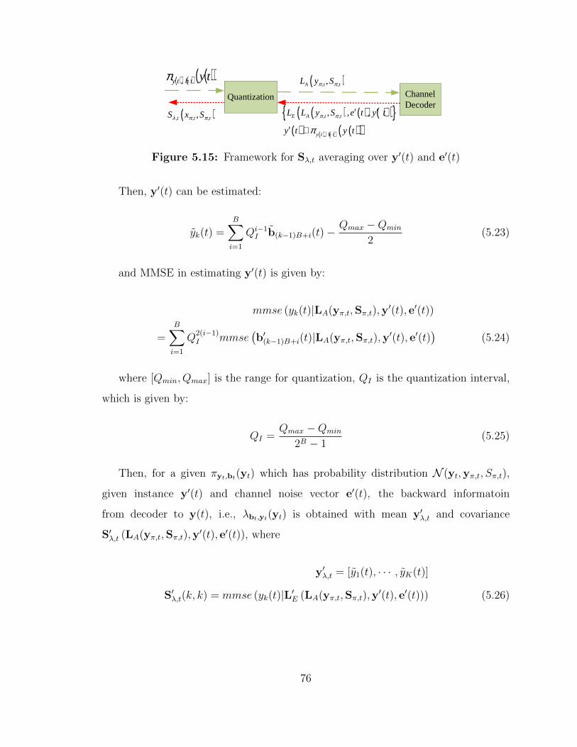
( ), , ,,t t tS x Sλ π π
Channel Decoder
Quantization
( ), ,,A t tL y Sπ π( ) ( ) ( )( )tytbty ,π
( ) ( ) ( )( ){ }( ) ( ) ( ) ( )( )
, ,
,
, , ,E A t t
y t b t
L L y S e t y t
y t y t
π π
π
′ ′
′ ∈
Figure 5.15: Framework for Sλ,t averaging over y′(t) and e′(t)
Then, y′(t) can be estimated:
yk(t) =B∑i=1
Qi−1I b(k−1)B+i(t)−
Qmax −Qmin
2(5.23)
and MMSE in estimating y′(t) is given by:
mmse (yk(t)|LA(yπ,t,Sπ,t),y′(t), e′(t))
=B∑i=1
Q2(i−1)I mmse
(b′(k−1)B+i(t)|LA(yπ,t,Sπ,t),y
′(t), e′(t))
(5.24)
where [Qmin, Qmax] is the range for quantization, QI is the quantization interval,
which is given by:
QI =Qmax −Qmin
2B − 1(5.25)
Then, for a given πyt,bt(yt) which has probability distribution N (yt,yπ,t, Sπ,t),
given instance y′(t) and channel noise vector e′(t), the backward informatoin
from decoder to y(t), i.e., λbt,yt(yt) is obtained with mean y′λ,t and covariance
S′λ,t (LA(yπ,t,Sπ,t),y′(t), e′(t)), where
y′λ,t = [y1(t), · · · , yK(t)]
S′λ,t(k, k) = mmse (yk(t)|L′E (LA(yπ,t,Sπ,t),y′(t), e′(t))) (5.26)
76

Channel Decoder
,tSπ
Quantization
( ), ,t tS Sλ π
( ){ }, ,,A t tL y Sπ π
( ) ( ) ( )( ){ }( ) ( ) ( ) ( )( ) ( )
( )
, ,
,
, , ,
,y t
E A t t
py t b t
L L y S e t y t
y t y t y t f
π π
ππ
′ ′
′ ∈ ∈
Figure 5.16: Framework for Sλ,t averaging over y′(t), e′(t) and yπ,t
Then, for a given πyt,bt(yt), extrinsic information transferred from decoder to y(t)
can be computed:
Sλ,t(yπ,t,Sπ,t) = Ey′t∈U(R(y)),e′(t)(LA(yπ,t,Sπ,t),y′(t), e′(t)) (5.27)
Denote the probability distribution of yπ,t as fyπ,t . Then, we can obtain average
Sπ,t, i.e., Sλ,t(Sπ,t) correponding to Sπ,t by integrating Sλ,t(yπ,t,Sπ,t) over yπ,t
Sλ,t(Sπ,t) = Eyπ,t (Sλ,t(yπ,t,Sπ,t))
= Eyπ,t
(Ey′t∈U(R(y)),e′(t)
(S′λ,t (LA(yπ,t,Sπ,t),y
′(t), e′(t))))
(5.28)
Note that the computation of Sλ,t(Sπ,t) requires serially averaging over y′(t) and
yπ,t. This is because that yπ,t not only impacts priori information LA(yπ,t,Sπ,t),
but also defines the set of codewords which are generated by quantizing y′(t). For
performance evaluation it means that the information transfer for the forward process
and backward process cannot be considered independently.
5.5.2 Approximation for the Information Exchange Between
State Estimator and Channel Decoder
As shown in above subsection, the computation of Sλ,t(Sπ,t) prohibits the independent
evaluation of the information transfer for forward process and backward process.
Forward process generally refers to message passing from a node to its children; and
backward process generally refers to message passing from a node to its parents.
77

Channel Decoder
,tSπ
Quantization
( ), ,t tS Sλ π
( ){ }, ,,A t tL y Sπ π
( ) ( ) ( )( ){ }( ) ( )( ) ( )
( )
, ,, , ,
,y t
E A t t
p
L L y S e t y t
y t U R y y t f
π π
π
′ ′
′ ∈ ∈
Figure 5.17: Approximate Framework 1 for Sλ,t averaging over y′(t), e′(t) and yπ,t
In this subsection, we make approximation for the computation of Sλ,t(Sπ,t) so that
the forward process and backward process can be considered separately.
Firstly, we integrate y′(t) over a uniform distribution instead of overN (yt,yπ,t,Sπ,t).
Denote the uniform distribution as U(R(y)), where R(y) is the range of y. Then, y′(t)
is independent of πyt,bt(yt); and the integration of y′(t) over U(R(y)) is equivalent
to the integration of all codewords with equal probability. Then,
Sλ,t(Sπ,t) ' Eyπ,t
(Ey′t∈U(R(y)),e′(t)
(S′λ,t (LA(yπ,t,Sπ,t),y
′(t), e′(t))))
= Eyπ,t,y′t∈U(R(y),e′(t)
(S′λ,t (LA(yπ,t,Sπ,t),y
′(t), e′(t)))
= ELA(yπ,t,Sπ,t),y′t∈U(R(y),e′(t)
(S′λ,t (LA(yπ,t,Sπ,t),y
′(t), e′(t)))
(5.29)
In the final step of Eq. 5.29, the avaraging over yπ,t is changed to avaraging over
LA(yπ,t,Sπ,t). This is because yπ,t impacts only priori information LA(yπ,t,Sπ,t) and
the set LA(yπ,t,Sπ,t) includes all information from yπ,t. The framework equivalent
with Eq. 5.29 is shown in Figure 5.17. In this new framework, the computation of
Sλ,t(Sπ,t) can be divided into three steps:
1. Step 1: compute the distribution of LA(yπ,t,Sπ,t corresponding to Sπ,t) and
fyπ,t ;
2. Step 2: compute the extrinsic information from channel decoder, i.e., the
distribution of L′E,i (LA(yπ,t,Sπ,t),y′(t), e′(t));
3. Step 3: compute Sλ,t(Sπ,t) from L′E,i (LA(yπ,t,Sπ,t),y′(t), e′(t)).
78

Channel Decoder
,tSπ
Quantization
( ), ,t tS Sλ π
AI
, BE extI MMSE
Figure 5.18: Approximate Framework 2 for Sλ,t averaging over y′(t), e′(t) and yπ,t
Secondly, we model the distribution of LA(yπ,t,Sπ,t) and L′E,i (LA(yπ,t,Sπ,t),y′(t), e′(t))
as Gaussian distribution with zero mean. Note that L′E,i (LA(yπ,t,Sπ,t),y′(t), e′(t))
for different bits might have huge difference. This Gaussian model requires a good
interleaver which can evenly distribute L′E,i (LA(yπ,t,Sπ,t),y′(t), e′(t)). Since LLR
with Guassian distribution can be represented by mutual information or MMSE
(Bhattad and Narayanan, 2007), Sλ,t(Sπ,t) can be computed in three steps as shown
in Figure 5.18:
1. Step 1: compute mutual information IA of the distribution of LA(yπ,t,Sπ,t)
corresponding to Sπ,t) and fyπ,t ;
2. Step 2: compute the extrinsic information from channel decoder, i.e., mutual in-
formation IE or MMSEBext of the distribution of L′E,i (LA(yπ,t,Sπ,t),y
′(t), e′(t));
3. Step 3: compute Sλ,t(Sπ,t) from extinsic information from channel decoder IE
or MMSEBext.
5.6 MSE-based Transfer Chart for Channel De-
coding and State Estimation
In the framework of BP based channel decoding and state estimation, the prediction
of y(t), i.e., πyt,bt(yt), is utilized to assist channel decoding in order to improve the
performanc of channel decoding. However, performance evaluation for this framework
is challenging because that the estimated y(t), i.e., λbt,yt(yt), is correlated with
predicted y(t),i.e., πyt,bt(yt). Instead of analytically evaluating the performance of
79
our proposed estimation scheme, we utilize the MSE-based transfer chart proposed by
(Guo et al., 2005) to evaluate its performance. By using MSE-based transfer chart,
the performance evaluation can be simplified; in addition, we can get visual insights
about the performance of our proposed estimation algorithm. The reason why we
select MSE as a measure is that it is aligned with one of the goal of state estimation,
i.e., minimizing the mse of estimated x(t). In this section, we show that how to obtain
MSE-based transfer for evaluating BP based sequential channel decoding and state
estimation as shown in Figure 5.8, and BP based iterative channel decoding and state
estimation as shown in Figure 5.9.
5.6.1 MSE-based Transfer Chart for Sequential Channel
Decoding and State Estimation over Time
In this subsection we demonstrate how to get MSE-based transfer for evaluating BP
based sequential channel decoding and state estimation as show in Figure 5.8. The
corresponding model for mse chart of sequential message passing is illusttrated in
Figure 5.19; and the MSE-based chart for BP based sequential channel decoding and
state estimation is the curve with MMSESap versus MMSES
ext. As shown in Figure 5.8,
the starting node is y(t); MMSESap is used to represent approximated Sπ,t, i.e.,
Sπ,t = MMSESapIK (5.30)
; and the distribution of yπ,t, i.e., fyπ,t , is assumed to keep the same in all time slots
and all iterations and denoted as fyπ . MMSESext is used to represent average Sπ,t+1
corresponding to Sπ,t equal to MMSESapIK and yπ,t with distribution fyπ . Comparing
with the model shown in Figure 5.8, the MSE-based chart has two differences. The
starting node for message passing is changed from x(t−1) to y(t). The reason for this
change is to keep aligns with the structure of MSE-based transfer chart for BP based
iterative channel decoding and state estimation. Note that x(t − 1) and y(t) can
80
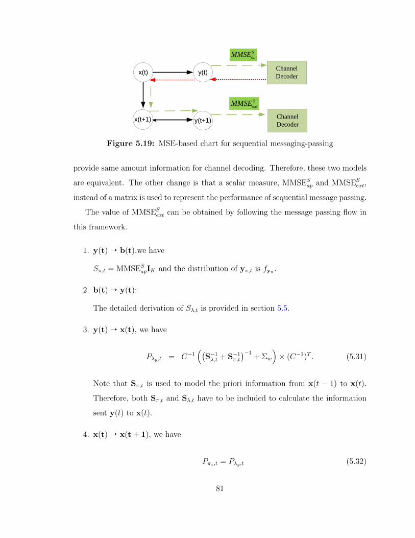
x(t) y(t)
x(t+1) y(t+1)
Channel Decoder
Channel Decoder
SapMMSE
SextMMSE
Figure 5.19: MSE-based chart for sequential messaging-passing
provide same amount information for channel decoding. Therefore, these two models
are equivalent. The other change is that a scalar measure, MMSESap and MMSES
ext,
instead of a matrix is used to represent the performance of sequential message passing.
The value of MMSESext can be obtained by following the message passing flow in
this framework.
1. y(t) Õ b(t),we have
Sπ,t = MMSESapIK and the distribution of yπ,t is fyπ .
2. b(t) Õ y(t):
The detailed derivation of Sλ,t is provided in section 5.5.
3. y(t) Õ x(t), we have
Pλy ,t = C−1((
S−1λ,t + S−1
π,t
)−1+ Σw
)× (C−1)T . (5.31)
Note that Sπ,t is used to model the priori information from x(t − 1) to x(t).
Therefore, both Sπ,t and Sλ,t have to be included to calculate the information
sent y(t) to x(t).
4. x(t) Õ x(t + 1), we have
Pπx,t = Pλy ,t (5.32)
81
5. x(t + 1) Õ y(t + 1), we have
Pπy ,t+1 = A× Pπx,t+1 × AT + Σp (5.33)
6. y(t + 1) Õ b(t + 1),we have
Sπ,t+1 = C × Pπy ,t+1 × CT + Σo (5.34)
Note that Sπ,t+1 is a matrix, MMSESext can be obtained by solving the following
equation:
IA(MMSESextIK) = IA(Sπ,t+1) (5.35)
The physical meaning of this equation is that MMSESext is the value such that
MMSESextIK can provide the same amount of priori information for channel
decoder as Sπ,t+1.
5.6.2 MSE-based Transfer Chart for BP Based Iterative
Channel Decoding and State Estimation Between Two
Time Slots
In this subsection, we illustrate how MSE-based transfer is modeled in order to
evaluate BP based iterative channel decoding and state estimation as shown in Figure
5.9. The corresponding model for MSE-based transfer chart is shown in Figure 5.20.
It includes two flows of message passing, the flow from y(t) to y(t + 1) as shown in
Figure 5.21 and the flow from y(t+ 1) to y(t) as shown in Figure 5.22.
1. Message passing flow from y(t) to y(t+ 1)
82

The starting node is y(t); and MMSEtap is used to represent approximated Sπ,t,
i.e.,
Sπ,t = MMSEtapIK (5.36)
; and the distribution of yπ,t, i.e., fyπ,t , is assumed to keep the same in all time
slots and all iterations and denoted as fyπ . MMSEtext is used to represent average
Sπ,t+1 corresponding to Sπ,t equal to MMSEtapIK and yπ,t with distribution fyπ .
2. Message passing flow from y(t+ 1) to y(t)
The starting node is y(t+ 1); and MMSEt+1ap is used to represent approximated
Sπ,t, i.e.,
Sπ,t+1 = MMSEt+1ap IK (5.37)
; and the distribution of yπ,t+1, i.e., fyπ,t+1 , is assumed to keep the same in
all time slots and all iterations and denoted as fyπ . MMSEt+1ext is used to
represent average Sπ,t corresponding to Sπ,t equal to MMSEt+1ap IK and yπ,t+1
with distribution fyπ .
Then, we have a curve with MMSEtap versus MMSEt
ext for messaging passing flow from
y(t) to y(t + 1); and flipped curve with MMSEt+1ext versus MMSEt+1
ap for messaging
passing flow from y(t+ 1) to y(t).
The value of MMSEextt can be obtained by following the message passing flow in
this framework.
1. y(t) Õ b(t),we have
Sπ,t = MMSEtapIK and the distribution of yπ,t is fyπ .
2. b(t) Õ y(t):
The detailed derivation of Sλ,t is provided in section 5.5.
83
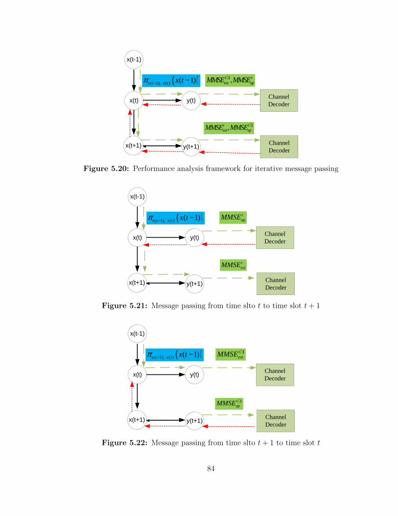
x(t-1)
x(t) y(t)
x(t+1) y(t+1)
Channel Decoder
Channel Decoder
( )( 1), ( ) ( 1)x t x t x tπ − − 1,t text apMMSE MMSE+
1,t text apMMSE MMSE +
Figure 5.20: Performance analysis framework for iterative message passing
x(t-1)
x(t) y(t)
x(t+1) y(t+1)
Channel Decoder
Channel Decoder
( )( 1), ( ) ( 1)x t x t x tπ − − tapMMSE
textMMSE
Figure 5.21: Message passing from time slto t to time slot t+ 1
x(t-1)
x(t) y(t)
x(t+1) y(t+1)
Channel Decoder
Channel Decoder
1textMMSE +
1tapMMSE +
( )( 1), ( ) ( 1)x t x t x tπ − −
Figure 5.22: Message passing from time slto t+ 1 to time slot t
84
3. y(t) Õ x(t), we have
Pλy ,t = C−1(Sλ,t + Σo)× (C−1)T . (5.38)
4. x(t) Õ x(t + 1), we have
Pπx,t = (P−1l,t + P−1
λ,t )−1 (5.39)
where
Pl,t = A× Pπx,t−1 × AT + Σp (5.40)
5. x(t + 1) Õ y(t + 1), we have
Pπy ,t+1 = A× Pπx,t+1 × AT + Σp (5.41)
6. y(t + 1) Õ b(t + 1),we have
Sπ,t+1 = C × Pπy ,t+1 × CT + Σo (5.42)
Note that Sπ,t+1 is a matrix, MMSEtext can be obtained by solving the following
equation:
IA(MMSEtextIK) = IA(Sπ,t+1) (5.43)
The physical meaning of this equation is that MMSEtext is the value such that
MMSEtextIK can provide the same amount of priori information for channel
decoder as Sπ,t+1.
The value of MMSEextt+1 can be obtained by following the message passing flow in
this framework.
85

1. y(t + 1) Õ b(t + 1),we have
Sπ,t+1 = MMSEt+1ap IK and the distribution of yπ,t+1 is fyπ .
2. b(t + 1) Õ y(t + 1):
The detailed derivation of Sλ,t+1 is provided in section 5.5.
3. y(t + 1) Õ x(t + 1), we have
Pλy ,t+1 = C−1(Sλ,t+1 + Σo)× (C−1)T . (5.44)
4. x(t + 1) Õ x(t), we have
Pλx,t = A−1(Σp + Pλy ,t+1)(A−1)T (5.45)
5. x(t) Õ y(t), we have
Pπy ,t = (P−1l,t + P−1
λx,t)−1 (5.46)
where
Pl,t = A× Pπx,t−1 × AT + Σp (5.47)
6. y(t) Õ b(t),we have
Sπ,t = C × Pπy ,t × CT + Σo (5.48)
Note that Sπ,t is a matrix, MMSEt+1ext can be obtained by solving the following
equation:
IA(MMSEt+1ext IK) = IA(Sπ,t) (5.49)
86

The physical meaning of this equation is that MMSEt+1ext is the value such that
MMSEt+1ext IK can provide the same amount of priori information for channel
decoder as Sπ,t.
5.7 Numerical Results
We consider the same electric generator dynamic system used for verification in
chapter 3. Each dimension of the observation yt is quantized with 14 bits, and the
dynamic range for quantization is [−432, 432]. A 1/2 rate Recursive Convolutional
(RSC) code is used as the channel coding scheme; and the code generator is
g = [1, 1, 1; 1, 0, 1]. The decoding algorithm is Log-Map algorithm.
The distribution of yπ,t, i.e., fyπ , is Gaussian with zero mean; and the covariance
matrix is obtained from the stationary distribution of y(t),
fyπ = N (y,0,Σyπ) (5.50)
where
Σyπ =
2857 0 0 0 0 0 0
0 6056 0 0 0 0 0
0 0 747 0 0 0 0
0 0 0 1624 0 0 0
0 0 0 0 44 0 0
0 0 0 0 0 10 0
0 0 0 0 0 0 0.79
(5.51)
In the model for BP based iterative channel decoding and state estimation, the
priori information from x(t− 1) to x(t) is a Gaussian distribution, i.e.,
πxt−1,xt(xt−1) = N (xt−1,xπx,t−1, Pπx,t−1) (5.52)
87

Channel Decoder
YapMMSE
Quantization
YextMMSE
AI
, BE extI MMSE
Figure 5.23: Model for message passing between state estimator and channeldecoder
where xπx,t−1 = 0 and Pπx,t−1 = MMSEt−1,xap IK .
5.7.1 Information Exchange Between State Estimator and
Channel Decoder
In this subsection we will show the performance evaluation results for message passing
between state estimator and channel decoder. In addition, we will demonstrate that
the gain of using redundancy of system dynamics to assist channel decoding can be
obtained by the proposed performance evaluation framework. The model shown in
Figure 5.23 is the approximation of the model shown in Figure 5.18 by setting Sπ,t
and Sλ,t as MMSEYapIK and MMSEY
extIK , respectively.
Figure 5.24 demonstrates the priori mutual information IA provided by different
MMSEYap. There are eight curves in this figure. The curve labeled with Di corresponds
to fyπ ,i which is a Gaussian distribution with zero mean and variance equal to ith
diagonal element of Σyπ . The curve labeled with mean correponds to fyπ which is a
Gaussian distribution with zero mean and covariance matrix equal to Σyπ . Note that
IA of curve labeled with mean is the average IA of curves labled with D1, · · · , D7.
When MMSEYap is equal to 1.0e − 1, 1.0, 1.0e + 1, 1.0e + 2, IA is equal to 0.55, 0.4,
0.25, 0.15, respectively. When MMSEYap is equal to 1.0e + 5, the prediction of y(t)
cannot provide any priori information for channel decoder since IA is equal to 0. Note
that although IA can be as high as 0.8 when MMSEYap is equal to 1.0e − 3, it is not
achievable as the minimum value of MMSEYap is limited by covariance matrix of state
dynamics and system observation noise, i.e, Σn and Σw, respectively.
88
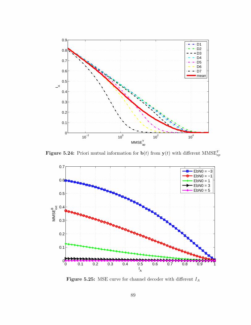
10−2
100
102
104
0
0.1
0.2
0.3
0.4
0.5
0.6
0.7
0.8
0.9
MMSEYap
I A
D1D2D3D4D5D6D7mean
Figure 5.24: Priori mutual information for b(t) from y(t) with different MMSEYap
0 0.1 0.2 0.3 0.4 0.5 0.6 0.7 0.8 0.9 10
0.1
0.2
0.3
0.4
0.5
0.6
0.7
IA
MM
SE
B ext
EbN0 = −3EbN0 = −1EbN0 = 1EbN0 = 3EbN0 = 5
Figure 5.25: MSE curve for channel decoder with different IA
89

10−2
100
102
104
10−2
100
102
104
106
MMSEYap
MM
SE
Y ext
EbN0 = −3EbN0 = −1EbN0 = 1EbN0 = 3EbN0 = 5
Figure 5.26: MMSEYext with different MMSEY
ap and Eb/N0
Figure 5.25 shows the relationship between extrinsic information in terms of
MMSE MMSEBext and priori information in terms of mutual information IA. Figure
5.26 illustrates the relationship between MMSEYap and MMSEY
ext. As shown in
Figure 5.24, the prediction of y(t) cannot provide any priori information for channel
decoder when MMSEYap is equal to 1.0e + 5. Therefore, when MMSEY
ap is equal to
1.0e+5, the corresponding MMSEYext is based on all information from channel decoder
without priori information from MMSEYext. Then, we can set the value of MMSEY
ext
corresponding to MMSEYap equal to 1.0e+ 5 as a reference value. For other MMSEY
ap
the gain can be obtained by comparing its MMSEYext with the reference MMSEY
ext.
The gain of MMSEYext with different MMSEY
ap and Eb/N0 is shown in Figure 5.27.
90

10−2
100
102
104
0
2
4
6
8
10
12
14
16
18
20
MMSEYap
Gai
n of
MM
SE
Y ext(d
B)
EbN0 = −3EbN0 = −1EbN0 = 1EbN0 = 3EbN0 = 5
Figure 5.27: Gain of MMSEYext with different MMSEY
ap and Eb/N0
5.7.2 Performance Analysis for Sequential Channle Decoding
and State Estimation
In this subsection, we will demonstrate how to use the proposed mse-based transfer
chart to evaluate the performance of BP based sequential channel decoding and state
estimation over time slots under different channel condition, which is modeled by
Eb/N0. Figure 5.28 shows the relationship between MMSESap and MMSES
ext with
different Eb/N0. In this figure, we have the following observations:
1. When MMSESap is less than 1, the corresponding MMSES
ext for all Eb/N0 are
equal.
Note that MMSESap is used to model the amount of priori information from
x(t − 1). Therefore, the smaller MMSESap is, the higher the amount of priori
information from x(t− 1) is. Although the extrinsic information from channel
decoder at time slot t can also contribute to the prediction of y(t+1), with small
91
MMSESap the priori information from x(t − 1) is dominant in the prediction of
y(t + 1). Therefore, the difference of gain from channel decoder with different
Eb/N0 is not seen in MMSESext.
2. With large MMSESap, the higher Eb/N0 is, the higher MMSES
ext is. This is
because that, with the increase of MMSESap, x(t − 1) provides less amount of
priori information for the prediction y(t) and the extrinsic information from
channel decoder becomes dominant in the prediction of y(t). Then, the channel
gain with different Eb/N0 is seen.
3. When MMSESap is around 1.0e− 2, there is floor for MMSES
ext.
It is because, based on information from time slots prior to t+ 1, the prediction
of y(t) cannot be accurate since state dynamics n(t) and the noise of system
observation w(t) are not predictable. Then, the minimum value of MMSESext is
limited by the covariance matrix of n(t) and w(t), i.e, Σn and Σw, respectively.
Following the idea of EXIT chart and MSE-based transfer chart for iterative
channel decoding, we use MSE-based transfer chart to evaluate the performance
of BP based channel decoding and state estimation over time slots. In the MSE-
based transfer chart we have two curves. One curve is MMSES,tap versus MMSES,t
ext
which is equivalent with the curve for MMSESap versus MMSES
ext in order to represent
the relationship between MMSESap and MMSES
ext at time slot t. The other curve
is MMSES,t+1ext versus MMSES,t+1
ap which is equivalent with flipped curve for MMSESap
versus MMSESext in order to represent the relationship between MMSES
ap and MMSESext
at time slot t+ 1.
The MSE-based transfer chart for Eb/N0 equal to 5dB is shown in Figure 5.29.
There is one cross point between these two curves, which is the convergence point.
The arrows with black color shows the trace of sequential message passing when
MMSESap is equal to 1.0e− 2 at time slot t. We can see that trace moves toward the
convergence point at time slot t+1 and t+2. The physical meaning is that even if we
92
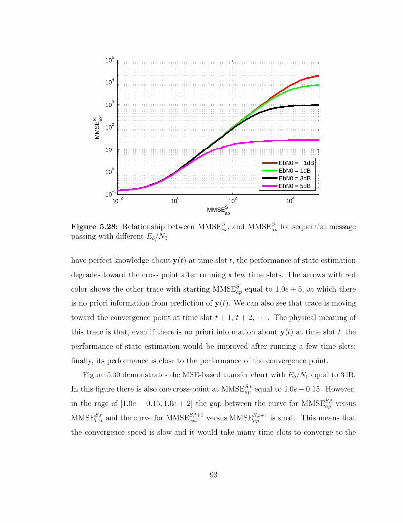
10−2
100
102
104
10−1
100
101
102
103
104
105
MMSESap
MM
SE
S ext
EbN0 = −1dBEbN0 = 1dBEbN0 = 3dBEbN0 = 5dB
Figure 5.28: Relationship between MMSESext and MMSES
ap for sequential messagepassing with different Eb/N0
have perfect knowledge about y(t) at time slot t, the performance of state estimation
degrades toward the cross point after running a few time slots. The arrows with red
color shows the other trace with starting MMSESap equal to 1.0e + 5, at which there
is no priori information from prediction of y(t). We can also see that trace is moving
toward the convergence point at time slot t+ 1, t+ 2, · · · . The physical meaning of
this trace is that, even if there is no priori information about y(t) at time slot t, the
performance of state estimation would be improved after running a few time slots;
finally, its performance is close to the performance of the convergence point.
Figure 5.30 demonstrates the MSE-based transfer chart with Eb/N0 equal to 3dB.
In this figure there is also one cross-point at MMSES,tap equal to 1.0e− 0.15. However,
in the rage of [1.0e − 0.15, 1.0e + 2] the gap between the curve for MMSES,tap versus
MMSES,text and the curve for MMSES,t+1
ext versus MMSES,t+1ap is small. This means that
the convergence speed is slow and it would take many time slots to converge to the
93

10−2
100
102
104
10−2
10−1
100
101
102
103
104
105
MMSES, tap
, MMSES, t+1ext
MM
SE
S, t
ext, M
MS
ES
, t+
1ap
MMSES,tap
vs MMSES,text
MMSES,t+1ext
vs MMSES,t+1ap
Cross−Point
Figure 5.29: MSE transfer chart for sequential channel decoding and stateestimation: Eb/N0 = 5dB
convergence point if the estimator has no priori information about y(t) at time slot
t.
Figure 5.31 and Figure 5.32 demonstrates the MSE-based transfer chart with
Eb/N0 equal to 1dB and -1dB, respectively. In these two figures there is also one
cross-point at MMSES,tap equal to 1.0e−0.15. However, after the cross-point the curve
for MMSES,tap versus MMSES,t
ext almost overlaps with the curve for MMSES,t+1ext versus
MMSES,t+1ap . Therefore, if the estimator has no priori information about y(t) at time
slot t, then it could either cannot converge to the cross-point and has high MSE or
it could take many time slots to converge to the cross-point. Therefore, for Eb/N0
equals to 1dB and -1dB, the MSE of estimating x(t) and y(t) is much higher than
that for Eb/N0 equal to 3dB and 5dB.
94

10−2
100
102
104
10−2
10−1
100
101
102
103
104
105
MMSES,tap
, MMSES,t+1ext
MM
SE
S,t
ext, M
MS
ES
,t+1
ap
MMSES,tap
vs MMSES,text
MMSES,t+1ext
vs MMSES,t+1ap
Cross−Point
Figure 5.30: MSE transfer chart for sequential channel decoding and stateestimation: Eb/N0 = 3dB
10−2
100
102
104
10−2
10−1
100
101
102
103
104
105
MMSES,tap
, MMSES,t+1ext
MM
SE
S,t
ext, M
MS
ES
,t+1
ap
MMSES,tap
vs MMSES,text
MMSES,t+1ext
vs MMSES,t+1ap
Cross−Point
Figure 5.31: MSE transfer chart for sequential channel decoding and stateestimation: Eb/N0 = 1dB
95
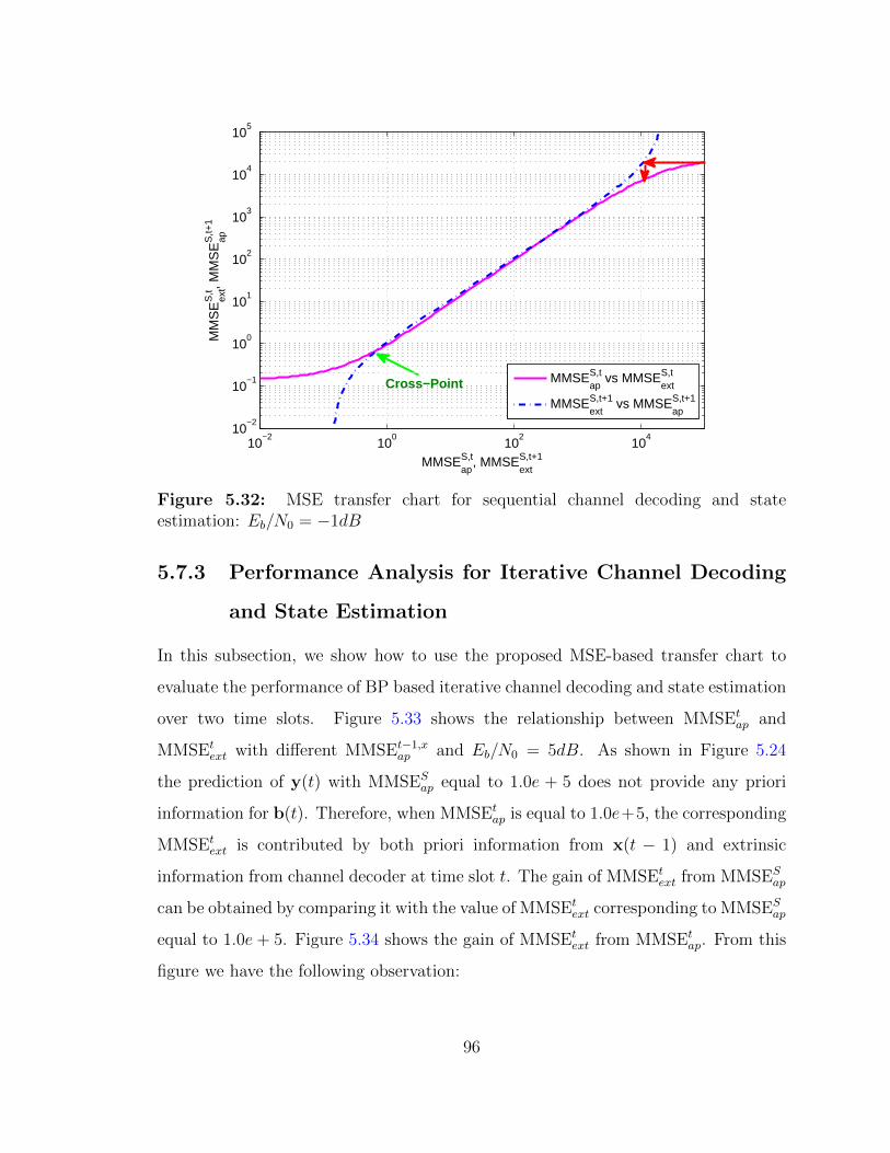
10−2
100
102
104
10−2
10−1
100
101
102
103
104
105
MMSES,tap
, MMSES,t+1ext
MM
SE
S,t
ext, M
MS
ES
,t+1
ap
MMSES,tap
vs MMSES,text
MMSES,t+1ext
vs MMSES,t+1ap
Cross−Point
Figure 5.32: MSE transfer chart for sequential channel decoding and stateestimation: Eb/N0 = −1dB
5.7.3 Performance Analysis for Iterative Channel Decoding
and State Estimation
In this subsection, we show how to use the proposed MSE-based transfer chart to
evaluate the performance of BP based iterative channel decoding and state estimation
over two time slots. Figure 5.33 shows the relationship between MMSEtap and
MMSEtext with different MMSEt−1,x
ap and Eb/N0 = 5dB. As shown in Figure 5.24
the prediction of y(t) with MMSESap equal to 1.0e + 5 does not provide any priori
information for b(t). Therefore, when MMSEtap is equal to 1.0e+5, the corresponding
MMSEtext is contributed by both priori information from x(t − 1) and extrinsic
information from channel decoder at time slot t. The gain of MMSEtext from MMSES
ap
can be obtained by comparing it with the value of MMSEtext corresponding to MMSES
ap
equal to 1.0e+ 5. Figure 5.34 shows the gain of MMSEtext from MMSEt
ap. From this
figure we have the following observation:
96
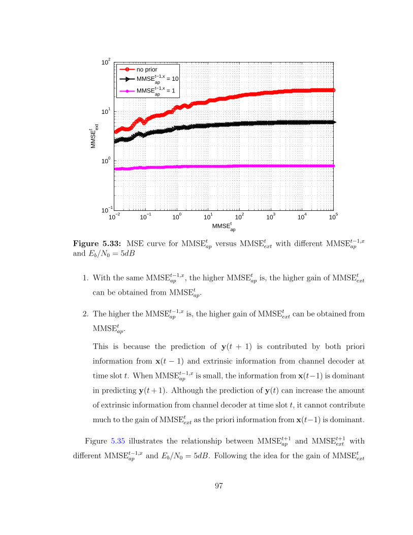
10−2
10−1
100
101
102
103
104
105
10−1
100
101
102
MMSEtap
MM
SE
t ext
no prior
MMSEt−1,xap
= 10
MMSEt−1,xap
= 1
Figure 5.33: MSE curve for MMSEtap versus MMSEt
ext with different MMSEt−1,xap
and Eb/N0 = 5dB
1. With the same MMSEt−1,xap , the higher MMSEt
ap is, the higher gain of MMSEtext
can be obtained from MMSEtap.
2. The higher the MMSEt−1,xap is, the higher gain of MMSEt
ext can be obtained from
MMSEtap.
This is because the prediction of y(t + 1) is contributed by both priori
information from x(t − 1) and extrinsic information from channel decoder at
time slot t. When MMSEt−1,xap is small, the information from x(t−1) is dominant
in predicting y(t+ 1). Although the prediction of y(t) can increase the amount
of extrinsic information from channel decoder at time slot t, it cannot contribute
much to the gain of MMSEtext as the priori information from x(t−1) is dominant.
Figure 5.35 illustrates the relationship between MMSEt+1ap and MMSEt+1
ext with
different MMSEt−1,xap and Eb/N0 = 5dB. Following the idea for the gain of MMSEt
ext
97
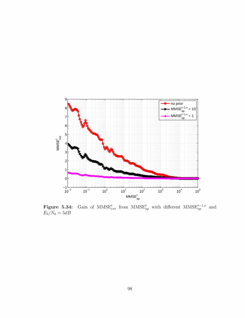
10−2
10−1
100
101
102
103
104
105
−1
0
1
2
3
4
5
6
7
8
9
MMSEtap
MM
SE
t ext
no prior
MMSEt−1,xap
= 10
MMSEt−1,xap
= 1
Figure 5.34: Gain of MMSEtext from MMSEt
ap with different MMSEt−1,xap and
Eb/N0 = 5dB
98

10−2
10−1
100
101
102
103
104
105
10−1
100
101
102
MMSEt+1ap
Gai
n of
MM
SE
t+1
ext
no prior
MMSEt−1,xap
= 10
MMSEt−1,xap
= 1
Figure 5.35: MSE curve for MMSEt+1ap versus MMSEt+1
ext with different MMSEt−1,xap
and Eb/N0 = 5dB
from MMSEtap, the gain of MMSEt+1
ext from MMSEt+1ap is obtained and shown in Figure
5.36. We have similar observation as the gain of MMSEtext from MMSEt
ap:
1. With the same MMSEt−1,xap , the higher MMSEt+1
ap is, the higher gain of MMSEt+1ext
can be obtained from MMSEtap.
2. The higher the MMSEt−1,xap is, the higher gain of MMSEt+1
ext can be obtained
from MMSEt+1ap .
We obtain the MSE-based transfer chart for BP based iterative channel decoding
and state estimation from the curve for MMSEtap versus MMSEt
ext and the curve for
MMSEt+1ap versus MMSEt+1
ext . Figure 5.37 demonstrates the MSE-based transfer chart
with different MMSEt−1,xap and Eb/N0 equals to 5dB. From this figure, for the case
without priori information from x(t− 1) we have the following observation:
99
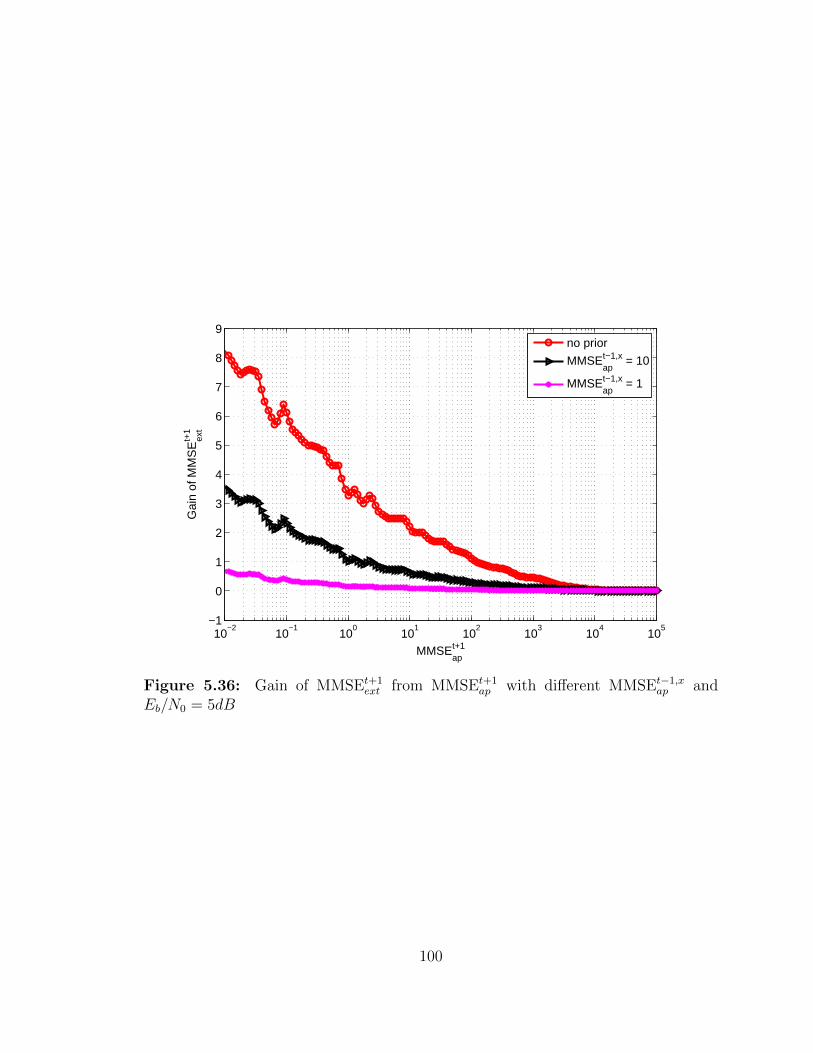
10−2
10−1
100
101
102
103
104
105
−1
0
1
2
3
4
5
6
7
8
9
MMSEt+1ap
Gai
n of
MM
SE
t+1
ext
no prior
MMSEt−1,xap
= 10
MMSEt−1,xap
= 1
Figure 5.36: Gain of MMSEt+1ext from MMSEt+1
ap with different MMSEt−1,xap and
Eb/N0 = 5dB
100

1. BP based iterative channel decoding can decrease MMSEtext and help improve
the estimation of x(t+ 1).
The cross-point between the curve for MMSEtap versus MMSEt
ext and the curve
for MMSEt+1ap versus MMSEt+1
ext is the convergence point of BP based iterative
channel decoding and state estimation. As shown in the figure, the value of
MMSEtap and MMSEt
ext corresponding to the cross-point are 1.0e + 1.33 and
1.0e+ 1.25, respectively; and the value of MMSEtext corresponding to the point
without priori information from y(t), i.e, MMSEtap = 1.0e + 5, is 1.0e + 1.43.
Therefore, the gain of MMSEtext for BP based iterative channel decoding and
state estimation is 10 ∗ (1.43− 1.25) = 1.8dB.
2. The gain of MMSEtext from BP based iterative channel decoding and state
estimation with three steps, step from y(t) to y(t + 1), step from y(t + 1) to
y(t), step from y(t) to y(t+ 1), is close to the gain of MMSEtext of convergence
point.
The trace of BP based iterative channel decoding and state estimation with the
mentioned three steps is shown by arrows with blue color in the figure. The
detail of these three steps is as below:
(a) Step 1: from y(t) to y(t+ 1):
As there is no priori information, the starting point is MMSEtap with value
1.0e+ 5; and the corresponding value of MMSEtext 1e+ 1.43.
(b) Step 2: y(t+ 1) to y(t):
We have MMSEt+1ap with value 1e + 1.43; and the corresponding value of
MMSEt+1ext is 1e+ 1.34
(c) Step 3: y(t) to y(t+ 1):
We have MMSEtap with value 1e + 1.34; and the corresponding value of
MMSEtext is 1e+1.255. Comparing with step 1, 10∗(1.43−1.255) =1.75dB
gain of MMSEtext is obtained from these three steps. Comparing with the
101
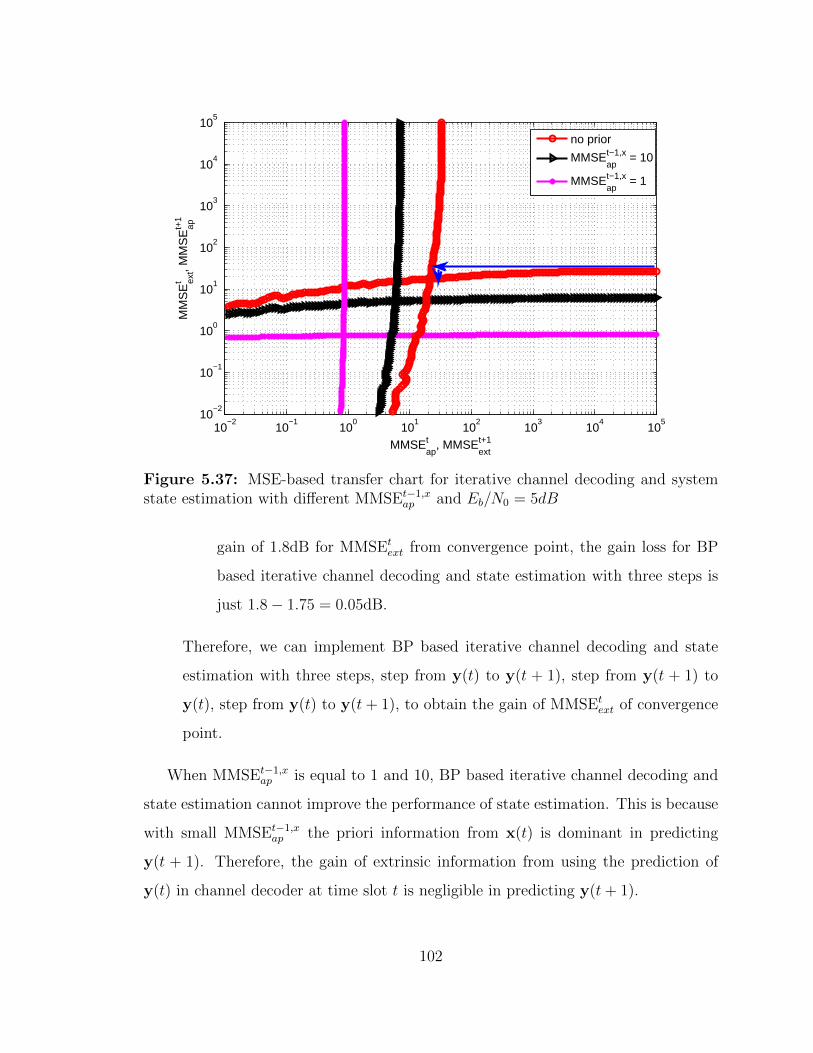
10−2
10−1
100
101
102
103
104
105
10−2
10−1
100
101
102
103
104
105
MMSEtap
, MMSEt+1ext
MM
SE
t ext, M
MS
Et+
1ap
no prior
MMSEt−1,xap
= 10
MMSEt−1,xap
= 1
Figure 5.37: MSE-based transfer chart for iterative channel decoding and systemstate estimation with different MMSEt−1,x
ap and Eb/N0 = 5dB
gain of 1.8dB for MMSEtext from convergence point, the gain loss for BP
based iterative channel decoding and state estimation with three steps is
just 1.8− 1.75 = 0.05dB.
Therefore, we can implement BP based iterative channel decoding and state
estimation with three steps, step from y(t) to y(t + 1), step from y(t + 1) to
y(t), step from y(t) to y(t+ 1), to obtain the gain of MMSEtext of convergence
point.
When MMSEt−1,xap is equal to 1 and 10, BP based iterative channel decoding and
state estimation cannot improve the performance of state estimation. This is because
with small MMSEt−1,xap the priori information from x(t) is dominant in predicting
y(t + 1). Therefore, the gain of extrinsic information from using the prediction of
y(t) in channel decoder at time slot t is negligible in predicting y(t+ 1).
102
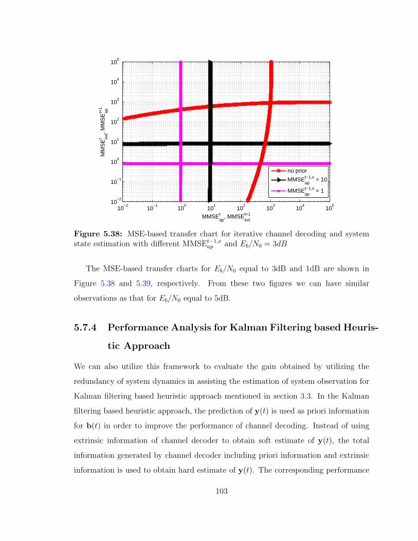
10−2
10−1
100
101
102
103
104
105
10−2
10−1
100
101
102
103
104
105
MMSEtap
, MMSEt+1ext
MM
SE
t ext, M
MS
Et+
1ap
no prior
MMSEt−1,xap
= 10
MMSEt−1,xap
= 1
Figure 5.38: MSE-based transfer chart for iterative channel decoding and systemstate estimation with different MMSEt−1,x
ap and Eb/N0 = 3dB
The MSE-based transfer charts for Eb/N0 equal to 3dB and 1dB are shown in
Figure 5.38 and 5.39, respectively. From these two figures we can have similar
observations as that for Eb/N0 equal to 5dB.
5.7.4 Performance Analysis for Kalman Filtering based Heuris-
tic Approach
We can also utilize this framework to evaluate the gain obtained by utilizing the
redundancy of system dynamics in assisting the estimation of system observation for
Kalman filtering based heuristic approach mentioned in section 3.3. In the Kalman
filtering based heuristic approach, the prediction of y(t) is used as priori information
for b(t) in order to improve the performance of channel decoding. Instead of using
extrinsic information of channel decoder to obtain soft estimate of y(t), the total
information generated by channel decoder including priori information and extrinsic
information is used to obtain hard estimate of y(t). The corresponding performance
103

10−2
10−1
100
101
102
103
104
105
10−2
10−1
100
101
102
103
104
105
MMSEtap
, MMSEt+1ext
MM
SE
t ext, M
MS
Et+
1ap
no prior
MMSEt−1,xap
= 10
MMSEt−1,xap
= 1
Figure 5.39: MSE-based transfer chart for iterative channel decoding and systemstate estimation with different MMSEt−1,x
ap and Eb/N0 = 1dB
Channel Decoder
YapMMSE
Quantization
YtotMMSE
AI
BtotMMSE
Figure 5.40: Model for message passing between state estimator and channeldecoder
104
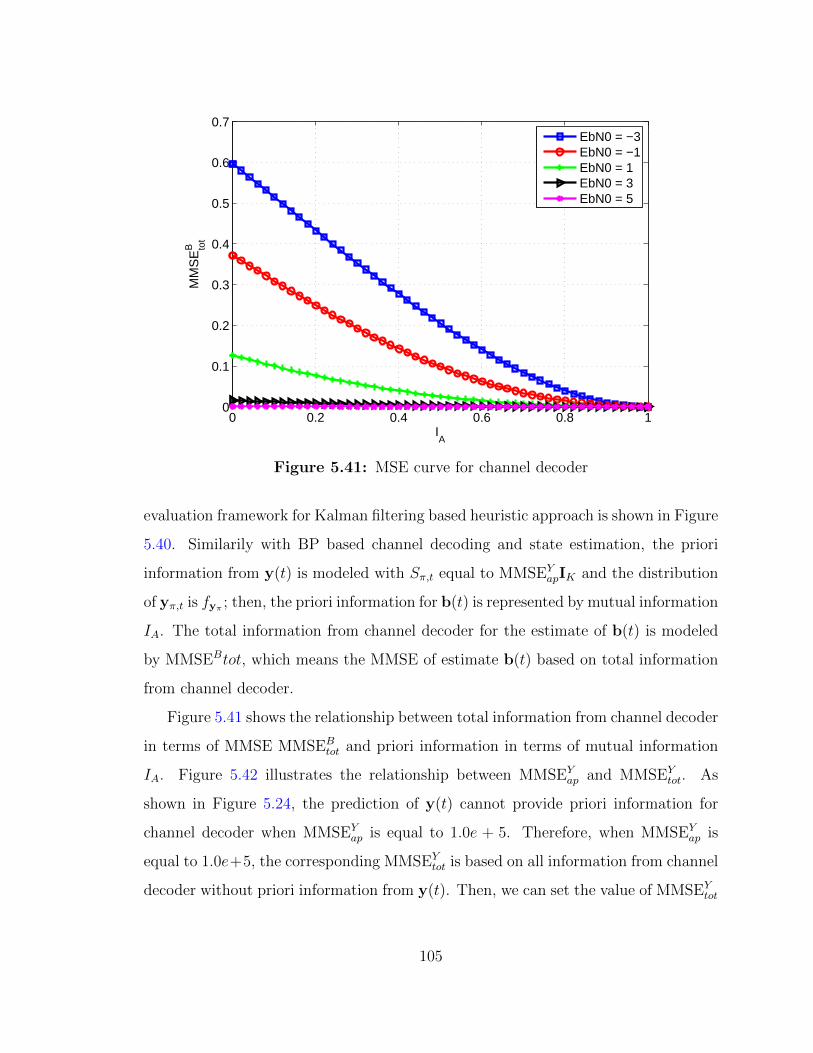
0 0.2 0.4 0.6 0.8 10
0.1
0.2
0.3
0.4
0.5
0.6
0.7
IA
MM
SE
B tot
EbN0 = −3EbN0 = −1EbN0 = 1EbN0 = 3EbN0 = 5
Figure 5.41: MSE curve for channel decoder
evaluation framework for Kalman filtering based heuristic approach is shown in Figure
5.40. Similarily with BP based channel decoding and state estimation, the priori
information from y(t) is modeled with Sπ,t equal to MMSEYapIK and the distribution
of yπ,t is fyπ ; then, the priori information for b(t) is represented by mutual information
IA. The total information from channel decoder for the estimate of b(t) is modeled
by MMSEBtot, which means the MMSE of estimate b(t) based on total information
from channel decoder.
Figure 5.41 shows the relationship between total information from channel decoder
in terms of MMSE MMSEBtot and priori information in terms of mutual information
IA. Figure 5.42 illustrates the relationship between MMSEYap and MMSEY
tot. As
shown in Figure 5.24, the prediction of y(t) cannot provide priori information for
channel decoder when MMSEYap is equal to 1.0e + 5. Therefore, when MMSEY
ap is
equal to 1.0e+5, the corresponding MMSEYtot is based on all information from channel
decoder without priori information from y(t). Then, we can set the value of MMSEYtot
105
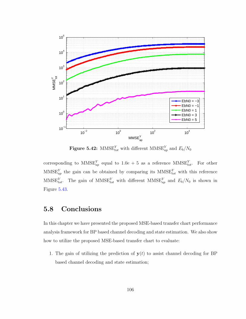
10−2
100
102
104
10−1
100
101
102
103
104
105
MMSEYap
MM
SE
Y tot
EbN0 = −3EbN0 = −1EbN0 = 1EbN0 = 3EbN0 = 5
Figure 5.42: MMSEYtot with different MMSEY
ap and Eb/N0
corresponding to MMSEYap equal to 1.0e + 5 as a reference MMSEY
tot. For other
MMSEYap the gain can be obtained by comparing its MMSEY
tot with this reference
MMSEYtot. The gain of MMSEY
tot with different MMSEYap and Eb/N0 is shown in
Figure 5.43.
5.8 Conclusions
In this chapter we have presented the proposed MSE-based transfer chart performance
analysis framework for BP based channel decoding and state estimation. We also show
how to utilize the proposed MSE-based transfer chart to evaluate:
1. The gain of utilizing the prediction of y(t) to assist channel decoding for BP
based channel decoding and state estimation;
106

10−2
100
102
104
0
2
4
6
8
10
12
14
16
18
20
MMSEYap
Gai
n of
MM
SE
Y tot(d
B)
EbN0 = −3EbN0 = −1EbN0 = 1EbN0 = 3EbN0 = 5
Figure 5.43: Gain of MMSEYtot with different MMSEY
ap and Eb/N0
2. the performance of BP based sequential channel decoding and state estimation
over time slots with channel condition modeled by Eb/N0;
3. the performance of BP based iterative channel decoding and state estimation
over two time slots;
4. the gain of utilizing the prediction of y(t) to assist channel decoding for Kalman
filtering based heuristic approach for state estimation.
107
Chapter 6
Conclusions and Future Work
6.1 Summary of Contributions
In this dissertation we study the decoding procedure (including the demodulation
procedure) for the messages with no or weak channel coding protection in the context
of NCS with stringent delay requirement. We propose to utilize the redundancy of
the system dynamics to protect the reliability of the uncoded or weakly encoded
messages. The system dynamics are considered as a ‘nature encoding’ similar to
convolution code, due to its redundancy in time.
Firstly, for systems with or without explicit channel coding, a decoding procedures
based on Pearl’s Belief Propagation (BP), in a similar manner to Turbo processing
in traditional data communication systems, is proposed. Numerical simulations have
demonstrated the validity of the schemes, using a linear model of electric generator
dynamic system. One disadvantage of this proposed scheme is that there is error
propagation at low SNR especially for Kalman Filtering based heuristic approach.
Secondly, we propose a quickest detection based error propagation detection
scheme to detect error propagation online. Then we combine this proposed error
propagation detection scheme with the proposed system dynamics assisted channel
decoding and state estimation algorithm to improve its robustness. The numerical
108
results show that error propagation does not happen and consistent performance
gain is observed in the proposed system dynamics based channel decoding and state
estimation together with error propagation detection.
Finally, we propose to use MSE-based transfer chart evaluate the performance
of BP based channel decoding and state estimation. We focus on two models, BP
based sequential and iterative channel decoding and state estimation. The first
model can be used to evaluate the performance of sequential channel decoding and
state estimation over time slots; and the second model can be used to evaluate
the performance of iterative channel decoding and state estimation over two time
slots. The numerical results show that MSE-based transfer chart can provide much
insight about the performance of the proposed BP based channel decoding and state
estimation algorithm.
6.2 Future Work
In this dissertation we propose to utilize the time-domain redundancy of system
dynamics to assist channel decoding; and propose an mse-based transfer performance
evaluation framework to jointly evaluate the performance of estimator and channel
decoder. In the future, more research work in the following areas can be performed.
1. Performance gain from system dynamics assisted channel decoding for estimator
discarding erroneous packets.
As shown in subsection 5.7.4 there is also gain from using system dynamics
to assist channel decoding on the condition that the prediction is correct
in probabilistic manner. The framework to utilize system dynamics assisted
channel decoding for estimator discarding erroneous packets is shown in Fig.6.1.
Estimator which discards erroneous packet is not impacted by communication
noise from estimates of system observation; therefore, estimator can provide
correct prediction for channel decoder in probabilistic manner resulting in
109
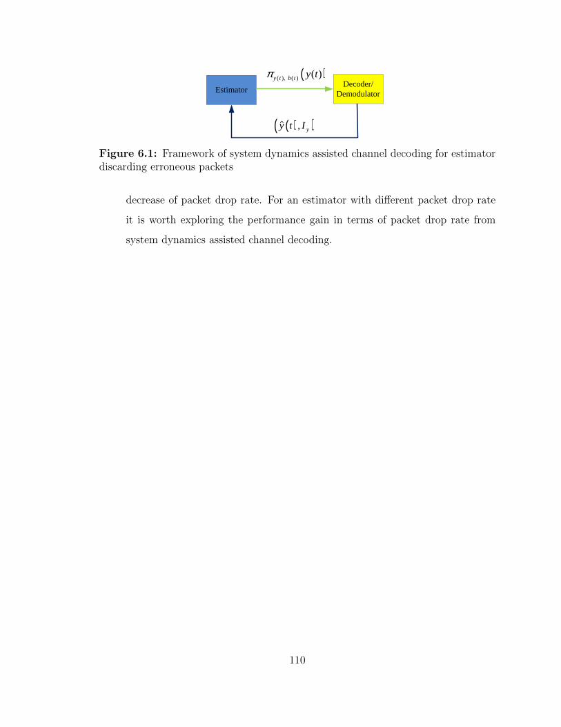
EstimatorDecoder/
Demodulator
( )( ), ( ) ( )y t b t y tπ
( )( )ˆ , yy t I
Figure 6.1: Framework of system dynamics assisted channel decoding for estimatordiscarding erroneous packets
decrease of packet drop rate. For an estimator with different packet drop rate
it is worth exploring the performance gain in terms of packet drop rate from
system dynamics assisted channel decoding.
110

Bibliography
111
Alexander, H. L. (1991). State estimation for distributed systems with sensing delay.
Proc. SPIE, 1470:103–111. 8
Alexander, P. D., Reed, M. C., and Schlegel, C. B. (1999). Iterative multiuser
interference reduction: Turbo cdma. IEEE Trans. Commun, 47(7):1008–1014. 5,
19
Ashikhmin, A., Kramer, G., and ten Brink, S. (2004). Extrinsic information
transfer functions: model and erasure channel properties. IEEE Trans. Inf. theory,
50(1):2657–2673. 16, 58
Bai, J., Eyisi, E., Qiu, F., Xue, Y., and Koutsoukos, X. (2012). Optimal cross-layer
design of sampling rate adaptation and network scheduling for wireless networked
control systems. In Cyber-Physical Systems (ICCPS), 2012 IEEE/ACM Third
International Conference on, pages 107–116. 10
Benedetto, S., Divsalar, D.and Montorsi, G., and Pollara, F. (1998). Serial
concatenation of interleaved codes: performance, analysis, design, and iterative
decoding. IEEE Trans. Inform. Theory, 44(3):909–926. 15
Berrou, C., Glavieux, A., and Thitimajshima, P. (1993). Near shannon limit error-
correcting coding and decoding. turbo codes. Proc. Int. Conf. Communications. 5,
19, 28
Bhattad, K. and Narayanan, K. R. (2007). An mse-based transfer chart for analyzing
iterative decoding schemes using a gaussian approximation. IEEE Trans. Inf.
theory, 53(1):22–38. 16, 29, 56, 58, 75, 79
Boggia, G., Camarda, P., Grieco, L., and Zacheo, G. (2008). Toward wireless
networked control systems: An experimental study on real-time communications
in 802.11 wlans. In Factory Communication Systems, 2008. WFCS 2008. IEEE
International Workshop on, pages 149–155. 2
112

Branicky, M. (1997). Stability of hybrid systems: state of the art. In Decision and
Control, 1997., Proceedings of the 36th IEEE Conference on, volume 1, pages 120–
125 vol.1. 13
Branicky, M. S., Phillips, S. M., and Zhang, W. (2000). Stability of networked control
systems: Explicit analysis of delay. In Proc. Amer. Contr. Conf., page 2352C2357.
13
Chamaken, A. and Litz, L. (2010). Joint design of control and communication in
wireless networked control systems: A case study. In American Control Conference
(ACC), 2010, pages 1835–1840. 10
Chen, S.and Lee, H., Chen, C., Huang, H., and Luo, C. (2007). Wireless sensor
network system by separating control and data path (scdp) for bio-medical
applications. In Microwave Conference, 2007. European, pages 430–433. 2
Chen, S.-L., Lee, H.-Y., Chen, C.-A., Huang, H.-Y., and Luo, C.-H. (2009). Wireless
body sensor network with adaptive low-power design for biometrics and healthcare
applications. Systems Journal, IEEE, 3(4):398–409. 2
Chen, W., Chen, L., Chen, Z., and Tu, S. (2005). A realtime dynamic traffic control
system based on wireless sensor network. In Parallel Processing, 2005. ICPP 2005
Workshops. International Conference Workshops on, pages 258–264. 2
Chen, Z., Weng, J., Yang, X., and Feng, J. (2011). Irrigation pumping station wireless
measurement and control system based on zigbee and 3g network. In Internet
Technology and Applications (iTAP), 2011 International Conference on, pages 1–
5. 2
Chiuso, A. and Schenato, L. (2008). Information fusion strategies from distributed
filters in packet-drop networks. In Decision and Control, 2008. CDC 2008. 47th
IEEE Conference on, pages 1079–1084. 10
113

Cover, T. M. and Thomas, J. A. (1991). Elements of information theory. Wiley. 11,
59
Duan, Z. and Li, X. (2011). Lossless linear transformation of sensor data for
distributed estimation fusion. Signal Processing, IEEE Transactions on, 59(1):362–
372. 10
Duan, Z. S., Li, X. R., and Yang, M. (2007). Why are more sensors better in
estimation fusion? In Proc. 2007 Int. Colloquium Information Fusion, pages 173
–179. 10
Elias, P. (1955). Coding for noise channels. IRE conv. Rept. Pr. 4, pages 37–47. 15
Fresia, M., Perez-Cruz, F., Poor, H. V., and Verdu, S. (2010). Joint source and
channel coding. IEEE Signal Processing Magzine, 27(6):104–113. 15, 17, 59
Gallager, R. G. (1963). Low-density parity-check codes. MIT Press, Cambridge, MA.
15, 16, 57, 62
Garcia-Frias, J. and Villasenor, J. D. (1997). Combining hidden markov source models
and parallel concatenated codes. IEEE Commun. Lett., 1(7):111–113. 15, 17, 59
Garcia-Frias, J. and Villasenor, J. D. (1998). Turbo decoding of hidden markov
sources with unknown parameters. Proc. of IEEE Data Compression Conf. 15, 17,
59
Garcia-Frias, J. and Villasenor, J. D. (2001). Joint turbo decoding and estimation of
hidden markov models. IEEE J. Select. Areas Commun., 19(9):1671–1679. 15, 17,
59
Garcia-Frias, J. and Zhao, Y. (2001). Data compression of unknown single and
correlated binary sources using punctured turbo codes. Proc. of 39th Annu. Allerton
Conf. Communications, Computing and Control. 15, 17, 59
114

Garcia-Frias, J. and Zhao, Y. (2002). Compression of binary memoryless sources
using punctured turbo codes. IEEE Commun. Lett., 6(9):394–396. 15, 17, 59
Garcia-Frias, J. and Zhong, W. (2003). Ldpc codes for compression of multi-terminal
sources with hidden markov correlation. IEEE Commun. Lett., 7(3):115–117. 15,
17, 59
Garcia-Frias, J., Zhong, W., and Zhao, Y. (2003). Turbo-like codes for source and
joint source-channel coding. Proc. of 3rd Int. Symp. Turbo Codes and Related
Topics. 15, 17, 59
Godoy, E., Scorzoni, F., and Porto, A. J. V. (2012). Evaluating serial zigbee devices
for application in wireless networked control systems. In IECON 2012 - 38th Annual
Conference on IEEE Industrial Electronics Society, pages 3176–3181. 2
Gong, S., Li, H., Lai, L., and Qiu, R. (2011). Decoding the ’nature encoded’ messages
for distributed energy generation control in microgrid. In Communications (ICC),
2011 IEEE International Conference on, pages 1–5. 33, 38
Guo, D., Shamai, S., and Verdu, S. (2005). Mutual information and mimimum mean-
square error in gaussian channels. IEEE Trans. Inf. theory, 51(4):1261–1281. 16,
17, 58, 62, 63, 80
Gupta, V., Chung, T. H., Hassibi, B., and Murray, R. M. (2006). On a stochastic
sensor selection algorithm with applications in sensor scheduling and sensor
coverage. Automatica, 42(2):251–260. 10
Gupta, V., Dana, A., Hespanha, J., Murray, R., and Hassibi, B. (2009). Data
transmission over networks for estimation and control. Automatic Control, IEEE
Transactions on, 54(8):1807–1819. 9, 10
Gupta, V., Hassibi, B., and Murray, R. M. (2007a). Optimal lqg control across
packet-dropping links. System and Control Letters, 56(6):439–446. 12
115
Gupta, V., Martins, N., and Baras, J. (2007b). Stabilization using multiple sensors
over analog erasure channels. In Modeling and Optimization in Mobile, Ad Hoc
and Wireless Networks and Workshops, 2007. WiOpt 2007. 5th International
Symposium on, pages 1–7. 12
Han, D. and Lim, J. (2010). Smart home energy management system using ieee
802.15.4 and zigbee. Consumer Electronics, IEEE Transactions on, 56(3):1403–
1410. 2
Heegard, C. and Wicker, S. (1999). Turbo coding. Kluwer International Series in
Engineering and Computer Science. Kluwer Academic, Boston. 15
Imer, O. C., Yuksel, S., and Basar, T. (2006). Optimal control of dynamical systems
over unreliable communication links. Automatica, 42(9):1429–1440. 8, 60
Jing, C., Shu, D., and Gu, D. (2007). Design of streetlight monitoring and
control system based on wireless sensor networks. In Industrial Electronics and
Applications, 2007. ICIEA 2007. 2nd IEEE Conference on, pages 57–62. 2
Kang, M., Ke, Y., and Li, J. (2011). Implementation of smart loading monitoring and
control system with zigbee wireless network. In 6th IEEE Conference on Industrial
Electronics and Applications (ICIEA), pages 907–912. 2
Kim, Y., Evans, R., and Iversen, W. (2008). Remote sensing and control of an
irrigation system using a distributed wireless sensor network. Instrumentation and
Measurement, IEEE Transactions on, 57(7):1379–1387. 2
Larsen, T., Andersen, N., Ravn, O., and Poulsen, N. (1998). Incorporation of time
delayed measurements in a discrete-time kalman filter. In Decision and Control,
1998. Proceedings of the 37th IEEE Conference on, volume 4, pages 3972–3977
vol.4. 8
116

Lee, S., Park, J., Ha, K., and Lee, K. (2008). Wireless networked control system
using ndis-based four-layer architecture for ieee 802.11b. In IEEE International
Workshop on Factory Communication Systems, pages 101–104. 2
Lin, H. and Antsaklis, P. (2004). Persistent disturbance attenuation properties for
networked control systems. In Decision and Control, 2004. CDC. 43rd IEEE
Conference on, volume 1, pages 953–958 Vol.1. 13
Lin, H. and Antsaklis, P. J. (2005). Stability and hinf performance preserving
scheduling policy for networked control systems. In In Proc. of the 16th World
Congress of Int. Federation of Automat. Contr. 13
Lin, H., Zhai, G., and Antsaklis, P. (2003). Robust stability and disturbance
attenuation analysis of a class of networked control systems. In Decision and
Control, 2003. Proceedings. 42nd IEEE Conference on, volume 2, pages 1182–1187
Vol.2. 13
Liu, Q., Wang, X., and Rao, N. S. V. (2012). Fusion of state estimates over long-haul
sensor networks under random delay and loss. In INFOCOM, 2012 Proceedings
IEEE, pages 2686–2690. 10
Liu, X. and Goldsmith, A. (2004). Kalman filtering with partial observation losses.
In Decision and Control, 2004. CDC. 43rd IEEE Conference on, volume 4, pages
4180–4186 Vol.4. 8
Ma, X., Djouadi, S., and Charalambous, C. (2011). Optimal filtering over uncertain
wireless communication channels. Signal Processing Letters, IEEE, 18(6):359–362.
8
Ma, X., Djouadi, S., Kuruganti, T., Nutaro, J., and Li, H. (2009). Optimal estimation
over unreliable communication links with application to cognitive radio. In Decision
and Control, 2009 held jointly with the 2009 28th Chinese Control Conference.
CDC/CCC 2009. Proceedings of the 48th IEEE Conference on, pages 4062–4067. 9
117

Ma, X., Djouadi, S., Kuruganti, T., Nutaro, J., and Li, H. (2010). Control and
estimation through cognitive radio with distributed and dynamic spectral activity.
In American Control Conference (ACC), 2010, pages 289–294. 9
Ma, X., Djouadi, S., and Li, H. (2012). State estimation over a semi-markov model
based cognitive radio system. Wireless Communications, IEEE Transactions on,
11(7):2391–2401. 9
Machowski, J., Bialek, J. W., and Bumby, J. R. (2008). Power system dynamics:
stability and control. Wiley. 31
Martins, N., Dahleh, M., and Elia, N. (2006). Feedback stabilization of uncertain
systems in the presence of a direct link. Automatic Control, IEEE Transactions
on, 51(3):438–447. 12
Matveev, A. and Savkin, A. (2003). The problem of state estimation via asynchronous
communication channels with irregular transmission times. Automatic Control,
IEEE Transactions on, 48(4):670–676. 8
McEliece, R., MacKay, D., and Cheng, J. (1998). Turbo decoding as an instance
of pearl’s ’belief propagation’ algorithm. IEEE Journal on selected areas in
communications, 16(2):140–152. 23
Mei, Z. and Wu, L. (2006). Joint source-channel decoding of huffman codes with ldpc
codes. J. Electron., 23(6):806–809. 15, 17, 59
Minero, P., Coviello, L., and Franceschetti, M. (2013). Stabilization over markov
feedback channels: the general case. Automatic Control, IEEE Transactions on,
58(2):349–362. 12, 59
Minero, P., Franceschetti, M., Dey, S., and Nair, G. (2009). Data rate theorem
for stabilization over time-varying feedback channels. Automatic Control, IEEE
Transactions on, 54(2):243–255. 12, 59
118

Mo, Y., Garone, E., Casavola, A., and Sinopoli, B. (2011). Stochastic sensor
scheduling for energy constrained estimation in multi-hop wireless sensor networks.
Automatic Control, IEEE Transactions on, 56(10):2489–2495. 10
Moayedi, M., Foo, Y., and Soh, Y. (2010). Adaptive kalman filtering in networked
systems with random sensor delays, multiple packet dropouts and missing
measurements. Signal Processing, IEEE Transactions on, 58(3):1577–1588. 9
Montestruque, L. and Antsaklis, P. (2002a). Model-based networked control systems:
necessary and sufficient conditions for stability. In 10th Mediterranean Conference
on Control and Automation. 14
Montestruque, L. and Antsaklis, P. (2002b). State and output feedback control in
model-based networked control systems. In Decision and Control, 2002, Proceedings
of the 41st IEEE Conference on, volume 2, pages 1620–1625 vol.2. 14
Montestruque, L. and Antsaklis, P. (2003a). On the model-based control of networked
systems. Automatica, 39(10):1837C1843. 14
Montestruque, L. and Antsaklis, P. (2003b). Stability of model-based networked
control systems with time-varying transmission times. In Proc. Amer. Contr. Conf.,
volume 5, page 4119C4124. 14
Montestruque, L. and Antsaklis, P. (2004). Stability of model-based networked
control systems with time-varying transmission times. Automatic Control, IEEE
Transactions on, 49(9):1562–1572. 14
Mostofi, Y. and Murray, R. (2004). Effect of time-varying fading channels on control
performance of a mobile sensor. In Sensor and Ad Hoc Communications and
Networks, 2004. IEEE SECON 2004. 2004 First Annual IEEE Communications
Society Conference on, pages 317–324. 60
119

Mostofi, Y. and Murray, R. (2009a). Kalman filtering over wireless fading channels.
Special Issue on Control with Limited Information, International Journal of Robust
and Nonlinear Control, 19:1993–2015. 9
Mostofi, Y. and Murray, R. (2009b). Kalman filtering over wireless fading channels
- how to handle packet drop. Special Issue on Control with Limited Information,
International Journal of Robust and Nonlinear Control, 19:1993–2015. 9, 60
Mostofi, Y. and Murray, R. (2009c). To drop or not to drop: Design principles
for kalman filtering over wireless fading channels. Automatic Control, IEEE
Transactions on, 54(2):376–381. 3, 9, 60
Nahi, N. (1969). Optimal recursive estimation with uncertain observation.
Information Theory, IEEE Transactions on, 15(4):457–462. 8
Nair, G. N. and Evans, R. J. (2004). Stabilizability of stochastic linear systems with
finite feedback data rates. SIAM J. Control Optimiz., 43(2):413C436. 12, 59
Nesic, D. and Teel, A. (2004). Input-output stability properties of networked control
systems. Automatic Control, IEEE Transactions on, 49(10):1650–1667. 14
Nilsson, J., Bernhardsson, B., and Wittenmark, B. (1998). Stochastic analysis and
control of real-time systems with random time delays. Automatica, 34(1):57–64. 8
Pan, X., Cuhadar, A., and Banihashemi, A. H. (2006). Combined source and channel
coding with jpeg2000 and rate-compatible low-density parity-check codes. IEEE
Trans. Signal Processing, 54(3):1160–1164. 15, 17, 59
Pearl, J. (1988). Probabilistic reasoning in intelligent systems: networks of plausible
inference. Morgan Kaufmann, San Mateo, CA. 23
Pu, L., Wu, Z., Bilgin, A., Marcellin, M. W., and Vasic, B. (2007). Ldpc-
based iterative joint source-channel decoding for jpeg2000. IEEE Trans. Image
Processing, 16(2):577–581. 15, 17, 59
120
Quevedo, D., Ahlen, A., and Ostergaard, J. (2010). Energy efficient state estimation
with wireless sensors through the use of predictive power control and coding. Signal
Processing, IEEE Transactions on, 58(9):4811–4823. 10
Quevedo, D., Ostergaard, J., and Ahlen, A. (2013). Power control and coding
formulation for state estimation with wireless sensors. Control Systems Technology,
IEEE Transactions on, PP(99):1–1. 10
Ramzan, N., Wan, S., and Izquierdo, E. (2007). Joint source-channel coding for
wavelet-based scalable video transmission using an adaptive turbo code. J. Image
Video Processing, 2007(1):1–12. 15, 17, 59
Refaat, T., Daoud, R., Amer, H., and Makled, E. (2010). Wifi implementation of
wireless networked control systems. In Networked Sensing Systems (INSS), 2010
Seventh International Conference on, pages 145–148. 2
Richardson, T. and Urbanke, R. (2001). The capacity of low-density parity check
codes under message passing decoding. IEEE Trans. Inform. Theory, 47:599–618.
23
Schenato, L. (2008). Optimal estimation in networked control systems subject
to random delay and packet drop. Automatic Control, IEEE Transactions on,
53(5):1311–1317. 8, 60
Schenato, L., Sinopoli, B., Franceschetti, M., Poolla, K., and Sastry, S. (2007).
Foundations of control and estimation over lossy networks. Proceedings of the
IEEE, 95(1):163–187. 60
Shannon, C. E. (1948). A mathematical theory of communication. Bell Syst. Tech.
J. 11
Sinopoli, B., Schenato, L., Franceschetti, M., Poolla, K., Jordan, M., and Sastry, S.
(2004). Kalman filtering with intermittent observations. Automatic Control, IEEE
Transactions on, 49(9):1453–1464. 8, 12, 60
121
Smith, S. and Seiler, P. (2003). Estimation with lossy measurements: jump estimators
for jump systems. Automatic Control, IEEE Transactions on, 48(12):2163–2171. 8
Song, J. (2010). Greenhouse monitoring and control system based on zigbee
wireless senor network. In 2010 International Conference on Electrical and Control
Engineering (ICECE), pages 2785–2788. 2
Song, Y. H., Park, J. H., Lee, K. Z., and Lee, S. (2009). Performance evaluation of
wireless networked control system using time-triggered ieee 802.15.4. In ICCAS-
SICE, pages 2187–2191. 2
Tatikonda, S. and Mitter, S. (2004). Control over noisy channels. Automatic Control,
IEEE Transactions on, 49(7):1196–1201. 11, 59
ten Brink, S. (1999). Convergence of iterative decoding. Electron. Lett., 35(1):1117–
1118. 16, 58, 62, 63
ten Brink, S. (2000). Iterative decoding trajectories of parallel concatenated codes.
Proc. 3rd IEEE/ITG Symp. Source and Channel Coding, pages 75–80. 16, 58, 62,
63
ten Brink, S. (2001). Convergence behavior of iteratively decoded parallel
concatenated codes. IEEE Trans. Commun, 49(10):1727–1737. 16, 58, 62, 63
Tuchler, M., Koetter., R., and Singer, A. C. (2002). Turbo equalization: principles
and new results. IEEE Trans. Commun, 50(5):754–767. 5, 19
Vembu, S., Verdu, S., and Steinberg, Y. (1995). The source-channel separation
theorem revisited. IEEE Trans. Inform. Theory, 41(1):44–54. 15
Walsh, G., Ye, H., and Bushnell, L. (2002). Stability analysis of networked control
systems. Control Systems Technology, IEEE Transactions on, 10(3):438–446. 14
122

Xu, Y. and Hespanha, J. (2004). Optimal communication logics in networked control
systems. In Decision and Control, 2004. CDC. 43rd IEEE Conference on, volume 4,
pages 3527–3532 Vol.4. 9, 10
Xu, Y. and Hespanha, J. (2005). Estimation under uncontrolled and controlled
communications in networked control systems. In Decision and Control, 2005
and 2005 European Control Conference. CDC-ECC ’05. 44th IEEE Conference
on, pages 842–847. 10
Xy, Y. and Hespanha, J. (2005). Estimation under uncontrolled and controlled
communications in networked control systems. In Decision and Control, 2005
and 2005 European Control Conference. CDC-ECC ’05. 44th IEEE Conference
on, pages 842–847. 9
Yang, C., Wu, J., Zhang, W., and Shi, L. (2013). Schedule communication
for decentralized state estimation. Signal Processing, IEEE Transactions on,
61(10):2525–2535. 10
Yen, B. X., Hop, D. T., and Yoo, M. (2013). Redundant transmission in wireless
networked control system over ieee 802.15.4e. In Information Networking (ICOIN),
2013 International Conference on, pages 628–631. 2
Yin, L., Lu, J., and Wu, Y. (2002). Ldpc-based joint source and channel coding
scheme for multimedia communications. Proc. of 8th Int. Conf. Communication
Systems. 15, 17, 59
Yook, J., Tilbury, D., and Soparkar, N. (2002). Trading computation for bandwidth:
reducing communication in distributed control systems using state estimators.
Control Systems Technology, IEEE Transactions on, 10(4):503–518. 10
You, K. and Xie, L. (2011). Minimum data rate for mean square stabilizability
of linear systems with markovian packet losses. Automatic Control, IEEE
Transactions on, 56(4):772–785. 12, 59
123

Zhai, G., Hu, B., Yasuda, K., and Michel, A. (2002). Qualitative analysis of discrete-
time switched systems. In American Control Conference, 2002. Proceedings of the
2002, volume 3, pages 1880–1885 vol.3. 13
Zhang, W., Branicky, M., and Phillips, S. (2001). Stability of networked control
systems. Control Systems, IEEE, 21(1):84–99. 13
Zhang, W. and Branicky, M. S. (2001). Stability of networked control systems with
time-varying transmission period. In in Allerton Conf. Communication, Contr. and
Computing. 14
Zhao, Y. and Garcia-Frias, J. (2002). Joint estimation and data compression
of correlated non-binary sources using punctured turbo codes. Proc. of Conf.
Information Sciences and Systems. 15, 17, 59
Zhao, Y. and Garcia-Frias, J. (2005). Joint estimation and compression of correlated
nonbinary sources using punctured turbo codes. IEEE Trans. Commun., 53(3):385–
390. 15, 17, 59
124

Appendix
125
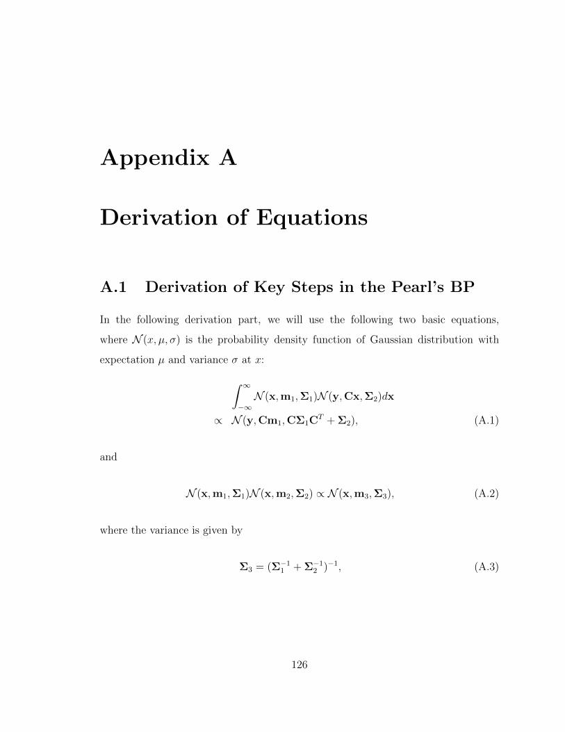
Appendix A
Derivation of Equations
A.1 Derivation of Key Steps in the Pearl’s BP
In the following derivation part, we will use the following two basic equations,
where N (x, µ, σ) is the probability density function of Gaussian distribution with
expectation µ and variance σ at x:
∫ ∞−∞N (x,m1,Σ1)N (y,Cx,Σ2)dx
∝ N (y,Cm1,CΣ1CT + Σ2), (A.1)
and
N (x,m1,Σ1)N (x,m2,Σ2) ∝ N (x,m3,Σ3), (A.2)
where the variance is given by
Σ3 = (Σ−11 + Σ−1
2 )−1, (A.3)
126
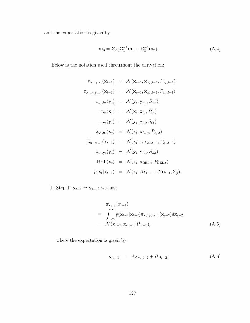
and the expectation is given by
m3 = Σ3(Σ−11 m1 + Σ−1
2 m2). (A.4)
Below is the notation used throughout the derivation:
πxt−1,xt(xt−1) = N (xt−1,xπx,t−1, Pπx,t−1)
πxt−1,yt−1(xt−1) = N (xt−1,xπy ,t−1, Pπy ,t−1)
πyt,bt(yt) = N (yt,yπ,t, Sπ,t)
πxt(xt) = N (xt,xl,t, Pl,t)
πyt(yt) = N (yt,yl,t, Sl,t)
λyt,xt(xt) = N (xt,xλy ,t, Pλy ,t)
λxt,xt−1(xt−1) = N (xt−1,xλx,t−1, Pλx,t−1)
λbt,yt(yt) = N (yt,yλ,t, Sλ,t)
BEL(xt) = N (xt,xBEL,t, PBEL,t)
p(xt|xt−1) = N (xt, Axt−1 +But−1,Σp).
1. Step 1: xt−1 Õ yt−1: we have
πxt−1(xt−1)
=
∫ ∞−∞
p(xt−1|xt−2)πxt−2,xt−1(xt−2)dxt−2
= N (xt−1,xl,t−1, Pl,t−1), (A.5)
where the expectation is given by
xl,t−1 = Axπx,t−2 +But−2, (A.6)
127

and the variance is given by
Pl,t−1 = A× Pπx,t−2 ×AT + Σp
πxt−1,yt−1(xt−1) = πxt−1(xt−1)λyt−1,xt−1(xt−1)
= N (xt−1,xl,t−1, Pl,t−1)× 1
= N (xt−1,xπy ,t−1, Pπy ,t−1) (A.7)
where
xπy ,t−1 = xl,t−1;Pπy ,t−1 = Pl,t−1. (A.8)
2. Step 2: yt−1 Õ bt−1:
πyt−1(yt−1) =
∫ ∞−∞
p(yt−1|xt−1)πxt−1,yt−1(xt−1)dxt−1
= N (yt−1 ,yl ,t−1 , Sl ,t−1 ) (A.9)
where
yl,t−1 = C × xπy ,t−1;
Sl,t−1 = C × Pπy ,t−1 × CT + Σo
πyt−1,bt−1(yt−1) = πyt−1(yt−1)× 1
= N (yt−1 ,yπ,t−1 , Sπ,t−1 ) (A.10)
where
yπ,t−1 = yl,t−1;
Sπ,t−1 = Sl,t−1 (A.11)
128

3. : Step 4: yt−1 Õ xt−1: we have
λyt−1,xt−1(xt−1) = γyt−1(xt−1)
=
∫ ∞−∞
λbt−1,yt−1(yt−1)p(yt−1|yx−1)
= N (xt−1,xλy ,t−1, Pλy ,t−1), (A.12)
where the expectation is given by
xλy ,t−1 = C−1 × yλ,t−1, (A.13)
and the variance is given by
Pλy ,t−1 = C−1(Sλ,t−1 + Σo)× (C−1)T . (A.14)
4. Step 5: xt−1 Õ xt: we have
πxt−1,xt(xt−1) = πxt−1(xt−1)× λyt−1,xt−1(xt−1)
= N (xt−1,xπx,t−1, Pπx,t−1), (A.15)
where the variance is given by
Pπx,t−1 = (P−1l,t−1 + P−1
λ,t−1)−1, (A.16)
and the expectation is given by
xπx,t−1 = Pπx,t−1 × (P−1l,t−1 × xl,t−1
+ P−1λ,t−1xλ,t−1).
129
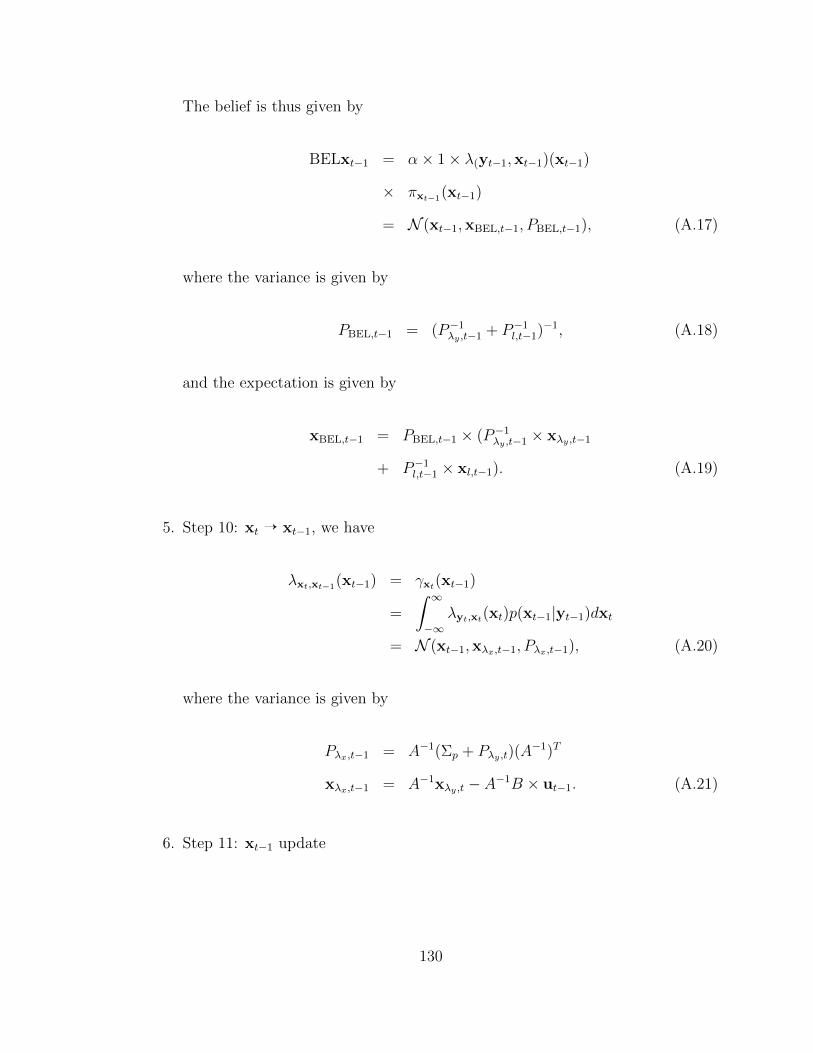
The belief is thus given by
BELxt−1 = α× 1× λ(yt−1,xt−1)(xt−1)
× πxt−1(xt−1)
= N (xt−1,xBEL,t−1, PBEL,t−1), (A.17)
where the variance is given by
PBEL,t−1 = (P−1λy ,t−1 + P−1
l,t−1)−1, (A.18)
and the expectation is given by
xBEL,t−1 = PBEL,t−1 × (P−1λy ,t−1 × xλy ,t−1
+ P−1l,t−1 × xl,t−1). (A.19)
5. Step 10: xt Õ xt−1, we have
λxt,xt−1(xt−1) = γxt(xt−1)
=
∫ ∞−∞
λyt,xt(xt)p(xt−1|yt−1)dxt
= N (xt−1,xλx,t−1, Pλx,t−1), (A.20)
where the variance is given by
Pλx,t−1 = A−1(Σp + Pλy ,t)(A−1)T
xλx,t−1 = A−1xλy ,t − A−1B × ut−1. (A.21)
6. Step 11: xt−1 update
130
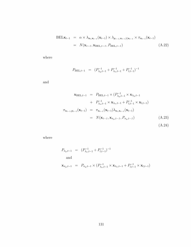
BELxt−1 = α× λxt,xt−1(xt−1)× λyt−1,xt−1)(xt−1 × πxt−1(xt−1)
= N (xt−1 ,xBEL,t−1 ,PBEL,t−1 ) (A.22)
where
PBEL,t−1 = (P−1λy ,t−1 + P−1
λx,t−1 + P−1l,t−1)−1
and
xBEL,t−1 = PBEL,t−1 × (P−1λy ,t−1 × xλy ,t−1
+ P−1λx,t−1 × xλx,t−1 + P−1
l,t−1 × xl,t−1)
πxt−1,yt−1(xt−1) = πxt−1(xt−1)λxt,xt−1(xt−1)
= N (xt−1 ,xπy ,t−1 ,Pπy ,t−1 ) (A.23)
(A.24)
where
Pπy ,t−1 = (P−1λx,t−1 + P−1
l,t−1)−1
and
xπy ,t−1 = Pπy ,t−1 × (P−1λx,t−1 × xλx,t−1 + P−1
l,t−1 × xl,t−1)
131
Vita
Shuping Gong was born in Yiyang, P.R. China. He received his B.S. degree in
electrical engineering from Hainan University in 2004, and his M.S. degree in electrical
engineering from University of Electronic Science and Technology of China in 2007.
From 2007 to 2008, he worked as an assistant engineer at Huawei Technologies
Co. Ltd, Shenzhen, P.R. China. He started his Ph.D. study at The University of
Tennessee, Knoxville, in January 2009. His current interests include integration of
wireless communication into Smart Grid and Cognitive Radio. Shuping is one of the
recipient of the Best Paper Awards of IEEE ICC in 2011. From January to August
2012, he worked as a student intern at Broadcom. Then, he joined Broadcom and
became a Staff II engineer. He will complete his Doctor of Philosophy degree in
Electrical Engineering in December 2013.
132