decision theory. Note - Brian Weatherson

Contents

1 Introduction 11.1 Decisions and Games . . . . . . . . . . . . . . . . . . . . . . . . . . . . . . . . . . . . . . . . . . . 1

1.2 Previews . . . . . . . . . . . . . . . . . . . . . . . . . . . . . . . . . . . . . . . . . . . . . . . . . . 2

1.3 Example: Newcomb . . . . . . . . . . . . . . . . . . . . . . . . . . . . . . . . . . . . . . . . . . . 3

1.4 Example: Sleeping Beauty . . . . . . . . . . . . . . . . . . . . . . . . . . . . . . . . . . . . . . . . 4

2 Simple Reasoning Strategies 52.1 Dominance Reasoning . . . . . . . . . . . . . . . . . . . . . . . . . . . . . . . . . . . . . . . . . . 5

2.2 States and Choices . . . . . . . . . . . . . . . . . . . . . . . . . . . . . . . . . . . . . . . . . . . . 5

2.3 Maximin and Maximax . . . . . . . . . . . . . . . . . . . . . . . . . . . . . . . . . . . . . . . . . . 6

2.4 Ordinal and Cardinal Utilities . . . . . . . . . . . . . . . . . . . . . . . . . . . . . . . . . . . . . . . 7

2.5 Regret . . . . . . . . . . . . . . . . . . . . . . . . . . . . . . . . . . . . . . . . . . . . . . . . . . . 8

2.6 Exercises . . . . . . . . . . . . . . . . . . . . . . . . . . . . . . . . . . . . . . . . . . . . . . . . . 9

3 Uncertainty 113.1 Likely Outcomes . . . . . . . . . . . . . . . . . . . . . . . . . . . . . . . . . . . . . . . . . . . . . 11

3.2 Do What’s Likely to Work . . . . . . . . . . . . . . . . . . . . . . . . . . . . . . . . . . . . . . . . 11

3.3 Probability and Uncertainty . . . . . . . . . . . . . . . . . . . . . . . . . . . . . . . . . . . . . . . . 13

4 Measures 154.1 Probability Defined . . . . . . . . . . . . . . . . . . . . . . . . . . . . . . . . . . . . . . . . . . . . 15

4.2 Measures . . . . . . . . . . . . . . . . . . . . . . . . . . . . . . . . . . . . . . . . . . . . . . . . . 15

4.3 Normalised Measures . . . . . . . . . . . . . . . . . . . . . . . . . . . . . . . . . . . . . . . . . . . 17

4.4 Formalities . . . . . . . . . . . . . . . . . . . . . . . . . . . . . . . . . . . . . . . . . . . . . . . . 17

4.5 Possibility Space . . . . . . . . . . . . . . . . . . . . . . . . . . . . . . . . . . . . . . . . . . . . . 18

5 Truth Tables 215.1 Compound Sentences . . . . . . . . . . . . . . . . . . . . . . . . . . . . . . . . . . . . . . . . . . . 21

5.2 Equivalence, Entailment, Inconsistency, and Logical Truth . . . . . . . . . . . . . . . . . . . . . . . 23

5.3 Two Important Results . . . . . . . . . . . . . . . . . . . . . . . . . . . . . . . . . . . . . . . . . . 25

6 Axioms for Probability 276.1 Axioms of Probability . . . . . . . . . . . . . . . . . . . . . . . . . . . . . . . . . . . . . . . . . . . 27

6.2 Truth Tables and Possibilities . . . . . . . . . . . . . . . . . . . . . . . . . . . . . . . . . . . . . . . 28

i

6.3 Propositions and Possibilities . . . . . . . . . . . . . . . . . . . . . . . . . . . . . . . . . . . . . . . 30

6.4 Exercises . . . . . . . . . . . . . . . . . . . . . . . . . . . . . . . . . . . . . . . . . . . . . . . . . 31

7 Conditional Probability 33

7.1 Conditional Probability . . . . . . . . . . . . . . . . . . . . . . . . . . . . . . . . . . . . . . . . . . 33

7.2 Bayes Theorem . . . . . . . . . . . . . . . . . . . . . . . . . . . . . . . . . . . . . . . . . . . . . . 34

7.3 Conditionalisation . . . . . . . . . . . . . . . . . . . . . . . . . . . . . . . . . . . . . . . . . . . . . 36

8 About Conditional Probability 39

8.1 Conglomerability . . . . . . . . . . . . . . . . . . . . . . . . . . . . . . . . . . . . . . . . . . . . . 39

8.2 Independence . . . . . . . . . . . . . . . . . . . . . . . . . . . . . . . . . . . . . . . . . . . . . . . 40

8.3 Kinds of Independence . . . . . . . . . . . . . . . . . . . . . . . . . . . . . . . . . . . . . . . . . . 40

8.4 Gamblers’ Fallacy . . . . . . . . . . . . . . . . . . . . . . . . . . . . . . . . . . . . . . . . . . . . . 42

9 Expected Utility 45

9.1 Expected Values . . . . . . . . . . . . . . . . . . . . . . . . . . . . . . . . . . . . . . . . . . . . . . 45

9.2 Maximise Expected Utility Rule . . . . . . . . . . . . . . . . . . . . . . . . . . . . . . . . . . . . . 46

9.3 Structural Features . . . . . . . . . . . . . . . . . . . . . . . . . . . . . . . . . . . . . . . . . . . . 48

10 Sure Thing Principle 51

10.1 Generalising Dominance . . . . . . . . . . . . . . . . . . . . . . . . . . . . . . . . . . . . . . . . . 51

10.2 Sure Thing Principle . . . . . . . . . . . . . . . . . . . . . . . . . . . . . . . . . . . . . . . . . . . 53

10.3 Allais Paradox . . . . . . . . . . . . . . . . . . . . . . . . . . . . . . . . . . . . . . . . . . . . . . . 54

10.4 Exercises . . . . . . . . . . . . . . . . . . . . . . . . . . . . . . . . . . . . . . . . . . . . . . . . . 56

11 Understanding Probability 57

11.1 Kinds of Probability . . . . . . . . . . . . . . . . . . . . . . . . . . . . . . . . . . . . . . . . . . . . 57

11.2 Frequency . . . . . . . . . . . . . . . . . . . . . . . . . . . . . . . . . . . . . . . . . . . . . . . . . 57

11.3 Degrees of Belief . . . . . . . . . . . . . . . . . . . . . . . . . . . . . . . . . . . . . . . . . . . . . 58

12 Objective Probabilities 61

12.1 Credences and Norms . . . . . . . . . . . . . . . . . . . . . . . . . . . . . . . . . . . . . . . . . . . 61

12.2 Evidential Probability . . . . . . . . . . . . . . . . . . . . . . . . . . . . . . . . . . . . . . . . . . . 62

12.3 Objective Chances . . . . . . . . . . . . . . . . . . . . . . . . . . . . . . . . . . . . . . . . . . . . 63

12.4 The Principal Principle and Direct Inference . . . . . . . . . . . . . . . . . . . . . . . . . . . . . . . 63

13 Understanding Utility 65

13.1 Utility and Welfare . . . . . . . . . . . . . . . . . . . . . . . . . . . . . . . . . . . . . . . . . . . . 65

13.2 Experiences and Welfare . . . . . . . . . . . . . . . . . . . . . . . . . . . . . . . . . . . . . . . . . 65

13.3 Objective List Theories . . . . . . . . . . . . . . . . . . . . . . . . . . . . . . . . . . . . . . . . . . 67

ii

14 Subjective Utility 6914.1 Preference Based Theories . . . . . . . . . . . . . . . . . . . . . . . . . . . . . . . . . . . . . . . . 69

14.2 Interpersonal Comparisons . . . . . . . . . . . . . . . . . . . . . . . . . . . . . . . . . . . . . . . . 70

14.3 Which Desires Count . . . . . . . . . . . . . . . . . . . . . . . . . . . . . . . . . . . . . . . . . . . 71

15 Declining Marginal Utilities 7315.1 Money and Utility . . . . . . . . . . . . . . . . . . . . . . . . . . . . . . . . . . . . . . . . . . . . . 73

15.2 Insurance . . . . . . . . . . . . . . . . . . . . . . . . . . . . . . . . . . . . . . . . . . . . . . . . . 74

15.3 Diversification . . . . . . . . . . . . . . . . . . . . . . . . . . . . . . . . . . . . . . . . . . . . . . . 74

15.4 Selling Insurance . . . . . . . . . . . . . . . . . . . . . . . . . . . . . . . . . . . . . . . . . . . . . 75

16 Newcomb’s Problem 7916.1 The Puzzle . . . . . . . . . . . . . . . . . . . . . . . . . . . . . . . . . . . . . . . . . . . . . . . . 79

16.2 Two Principles of Decision Theory . . . . . . . . . . . . . . . . . . . . . . . . . . . . . . . . . . . . 79

16.3 Bringing Two Principles Together . . . . . . . . . . . . . . . . . . . . . . . . . . . . . . . . . . . . 80

16.4 Well Meaning Friends . . . . . . . . . . . . . . . . . . . . . . . . . . . . . . . . . . . . . . . . . . . 82

17 Realistic Newcomb Problems 8317.1 Real Life Newcomb Cases . . . . . . . . . . . . . . . . . . . . . . . . . . . . . . . . . . . . . . . . 83

17.2 Tickle Defence . . . . . . . . . . . . . . . . . . . . . . . . . . . . . . . . . . . . . . . . . . . . . . 85

18 Causal Decision Theory 8718.1 Causal and Evidential Decision Theory . . . . . . . . . . . . . . . . . . . . . . . . . . . . . . . . . 87

18.2 Right and Wrong Tabulations . . . . . . . . . . . . . . . . . . . . . . . . . . . . . . . . . . . . . . . 87

18.3 Why Ain’Cha Rich . . . . . . . . . . . . . . . . . . . . . . . . . . . . . . . . . . . . . . . . . . . . 88

18.4 Dilemmas . . . . . . . . . . . . . . . . . . . . . . . . . . . . . . . . . . . . . . . . . . . . . . . . . 89

18.5 Weak Newcomb Problems . . . . . . . . . . . . . . . . . . . . . . . . . . . . . . . . . . . . . . . . 90

19 Introduction to Games 9119.1 Games . . . . . . . . . . . . . . . . . . . . . . . . . . . . . . . . . . . . . . . . . . . . . . . . . . . 91

19.2 Zero-Sum Games and Backwards Induction . . . . . . . . . . . . . . . . . . . . . . . . . . . . . . . 92

19.3 Zero-Sum Games and Nash Equilibrium . . . . . . . . . . . . . . . . . . . . . . . . . . . . . . . . . 94

20 Zero-Sum Games 9520.1 Mixed Strategies . . . . . . . . . . . . . . . . . . . . . . . . . . . . . . . . . . . . . . . . . . . . . 95

20.2 Surprising Mixed Strategies . . . . . . . . . . . . . . . . . . . . . . . . . . . . . . . . . . . . . . . . 96

20.3 Calculating Mixed Strategy Nash Equilibrium . . . . . . . . . . . . . . . . . . . . . . . . . . . . . . 97

21 Nash Equilibrium 9921.1 Illustrating Nash Equilibrium . . . . . . . . . . . . . . . . . . . . . . . . . . . . . . . . . . . . . . . 99

21.2 Why Play Equilibrium Moves? . . . . . . . . . . . . . . . . . . . . . . . . . . . . . . . . . . . . . . 100

21.3 Causal Decision Theory and Game Theory . . . . . . . . . . . . . . . . . . . . . . . . . . . . . . . . 102

iii

22 Many Move Games 10322.1 Games with Multiple Moves . . . . . . . . . . . . . . . . . . . . . . . . . . . . . . . . . . . . . . . 103

22.2 Extensive and Normal Form . . . . . . . . . . . . . . . . . . . . . . . . . . . . . . . . . . . . . . . 103

22.3 Two Types of Equilibrium . . . . . . . . . . . . . . . . . . . . . . . . . . . . . . . . . . . . . . . . 104

22.4 Normative Significance of Subgame Perfect Equilibrium . . . . . . . . . . . . . . . . . . . . . . . . 104

22.5 Cooperative Games . . . . . . . . . . . . . . . . . . . . . . . . . . . . . . . . . . . . . . . . . . . . 105

22.6 Pareto Efficient Outcomes . . . . . . . . . . . . . . . . . . . . . . . . . . . . . . . . . . . . . . . . 106

22.7 Exercises . . . . . . . . . . . . . . . . . . . . . . . . . . . . . . . . . . . . . . . . . . . . . . . . . 107

23 Backwards Induction 10923.1 Puzzles About Backwards Induction . . . . . . . . . . . . . . . . . . . . . . . . . . . . . . . . . . . 109

23.2 Pettit and Sugden . . . . . . . . . . . . . . . . . . . . . . . . . . . . . . . . . . . . . . . . . . . . . 111

24 Group Decisions 11324.1 Making a Decision . . . . . . . . . . . . . . . . . . . . . . . . . . . . . . . . . . . . . . . . . . . . 113

24.2 Desiderata for Preference Aggregation Mechanisms . . . . . . . . . . . . . . . . . . . . . . . . . . . 115

24.3 Assessing Plurality Voting . . . . . . . . . . . . . . . . . . . . . . . . . . . . . . . . . . . . . . . . 116

25 Arrow’s Theorem 11725.1 Ranking Functions . . . . . . . . . . . . . . . . . . . . . . . . . . . . . . . . . . . . . . . . . . . . 117

25.2 Cyclic Preferences . . . . . . . . . . . . . . . . . . . . . . . . . . . . . . . . . . . . . . . . . . . . 118

25.3 Proofs of Arrow’s Theorem . . . . . . . . . . . . . . . . . . . . . . . . . . . . . . . . . . . . . . . . 120

26 Voting Systems 12126.1 Plurality voting . . . . . . . . . . . . . . . . . . . . . . . . . . . . . . . . . . . . . . . . . . . . . . 121

26.2 Runoff Voting . . . . . . . . . . . . . . . . . . . . . . . . . . . . . . . . . . . . . . . . . . . . . . . 123

26.3 Instant Runoff Voting . . . . . . . . . . . . . . . . . . . . . . . . . . . . . . . . . . . . . . . . . . . 124

27 More Voting Systems 12527.1 Borda Count . . . . . . . . . . . . . . . . . . . . . . . . . . . . . . . . . . . . . . . . . . . . . . . . 125

27.2 Approval Voting . . . . . . . . . . . . . . . . . . . . . . . . . . . . . . . . . . . . . . . . . . . . . . 126

27.3 Range Voting . . . . . . . . . . . . . . . . . . . . . . . . . . . . . . . . . . . . . . . . . . . . . . . 127

iv

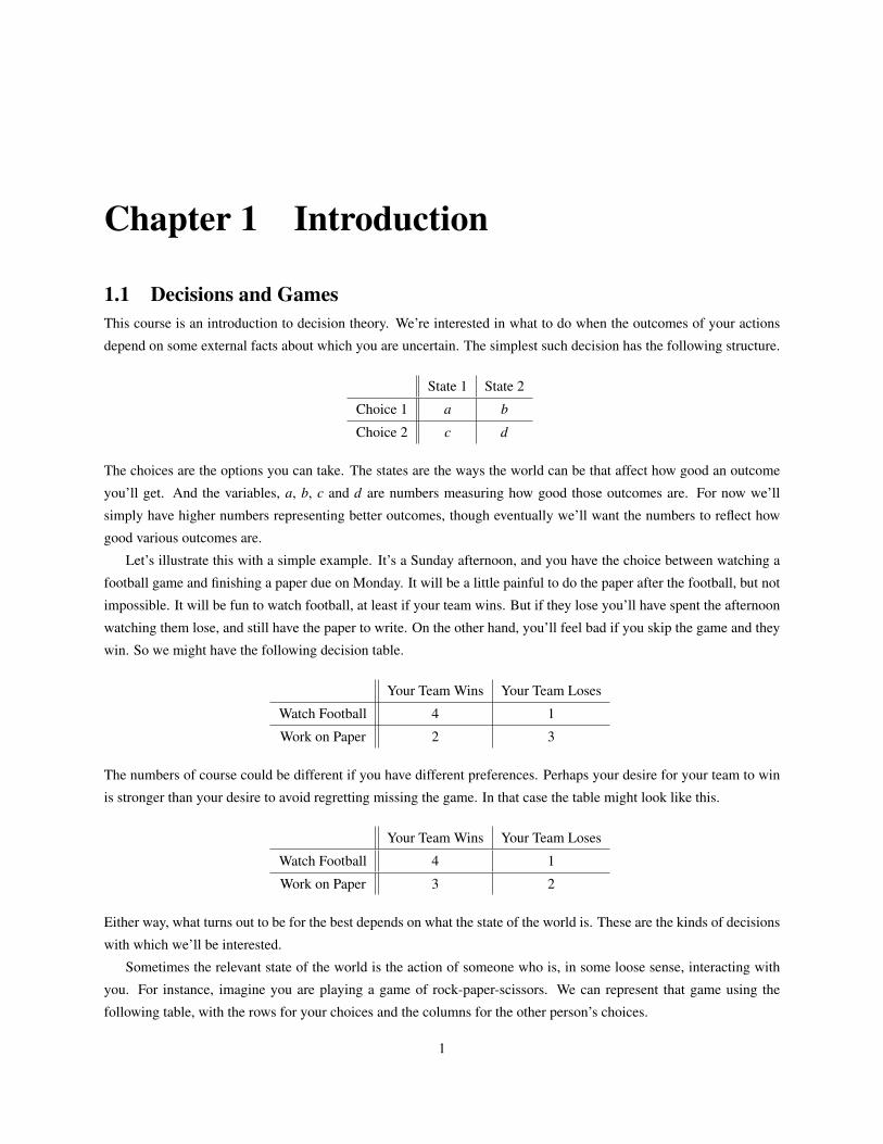
Chapter 1 Introduction

1.1 Decisions and GamesThis course is an introduction to decision theory. We’re interested in what to do when the outcomes of your actions

depend on some external facts about which you are uncertain. The simplest such decision has the following structure.

State 1 State 2

Choice 1 a b

Choice 2 c d

The choices are the options you can take. The states are the ways the world can be that affect how good an outcome

you’ll get. And the variables, a, b, c and d are numbers measuring how good those outcomes are. For now we’ll

simply have higher numbers representing better outcomes, though eventually we’ll want the numbers to reflect how

good various outcomes are.

Let’s illustrate this with a simple example. It’s a Sunday afternoon, and you have the choice between watching a

football game and finishing a paper due on Monday. It will be a little painful to do the paper after the football, but not

impossible. It will be fun to watch football, at least if your team wins. But if they lose you’ll have spent the afternoon

watching them lose, and still have the paper to write. On the other hand, you’ll feel bad if you skip the game and they

win. So we might have the following decision table.

Your Team Wins Your Team Loses

Watch Football 4 1

Work on Paper 2 3

The numbers of course could be different if you have different preferences. Perhaps your desire for your team to win

is stronger than your desire to avoid regretting missing the game. In that case the table might look like this.

Your Team Wins Your Team Loses

Watch Football 4 1

Work on Paper 3 2

Either way, what turns out to be for the best depends on what the state of the world is. These are the kinds of decisions

with which we’ll be interested.

Sometimes the relevant state of the world is the action of someone who is, in some loose sense, interacting with

you. For instance, imagine you are playing a game of rock-paper-scissors. We can represent that game using the

following table, with the rows for your choices and the columns for the other person’s choices.

1

1.2 Previews 1. Introduction

Rock Paper Scissors

Rock 0 -1 1

Paper 1 0 -1

Scissors -1 1 0

Not all games are competitive like this. Some games involve coordination. For instance, imagine you and a friend are

trying to meet up somewhere in New York City. You want to go to a movie, and your friend wants to go to a play, but

neither of you wants to go to something on their own. Sadly, your cell phone is dead, so you’ll just have to go to either

the movie theater or the playhouse, and hope your friend goes to the same location. We might represent the game you

and your friend are playing this way.

Movie Theater Playhouse

Movie Theater (2, 1) (0, 0)

Playhouse (0, 0) (1, 2)

In each cell now there are two numbers, representing first how good the outcome is for you, and second how good it is

for your friend. So if you both go to the movies, that’s the best outcome for you, and the second-best for your friend.

But if you go to different things, that’s the worst result for both of you. We’ll look a bit at games like this where the

party’s interests are neither strictly allied nor strictly competitive.

Traditionally there is a large division between decision theory, where the outcome depends just on your choice

and the impersonal world, and game theory, where the outcome depends on the choices made by multiple interacting

agents. We’ll follow this tradition here, focussing on decision theory for the first two-thirds of the course, and then

shifting our attention to game theory. But it’s worth noting that this division is fairly arbitrary. Some decisions depend

for their outcome on the choices of entities that are borderline agents, such as animals or very young children. And

some decisions depend for their outcome on choices of agents that are only minimally interacting with you. For these

reasons, among others, we should be suspicious of theories that draw a sharp line between decision theory and game

theory.

1.2 PreviewsJust thinking intuitively about decisions like whether to watch football, it seems clear that how likely the various states

of the world are is highly relevant to what you should do. If you’re more or less certain that your team will win, and

you’ll enjoy watching the win, then you should watch the game. But if you’re more or less certain that your team will

lose, then it’s better to start working on the term paper. That intuition, that how likely the various states are affects

what the right decision is, is central to modern decision theory.

The best way we have to formally regiment likelihoods is probability theory. So we’ll spend quite a bit of time

in this course looking at probability, because it is central to good decision making. In particular, we’ll be looking at

four things.

First, we’ll spend some time going over the basics of probability theory itself. Many people, most people in fact,

make simple errors when trying to reason probabilistically. This is especially true when trying to reason with so-called

conditional probabilities. We’ll look at a few common errors, and look at ways to avoid them.

2

1. Introduction 1.3 Example: Newcomb

Second, we’ll look at some questions that come up when we try to extend probability theory to cases where there

are infinitely many ways the world could be. Some issues that come up in these cases affect how we understand

probability, and in any case the issues are philosophically interesting in their own right.

Third, we’ll look at some arguments as to why we should use probability theory, rather than some other theory of

uncertainty, in our reasoning. Outside of philosophy it is sometimes taken for granted that we should mathematically

represent uncertainties as probabilities, but this is in fact quite a striking and, if true, profound result. So we’ll pay

some attention to arguments in favour of using probabilities. Some of these arguments will also be relevant to questions

about whether we should represent the value of outcomes with numbers.

Finally, we’ll look a little at where probabilities come from. The focus here will largely be negative. We’ll look

at reasons why some simple identifications of probabilities either with numbers of options or with frequencies are

unhelpful at best.

In the middle of the course, we’ll look at a few modern puzzles that have been the focus of attention in decision

theory. Later today we’ll go over a couple of examples that illustrate what we’ll be covering in this section.

The final part of the course will be on game theory. We’ll be looking at some of the famous examples of two

person games. (We’ve already seen a version of one, the movie and play game, above.) And we’ll be looking at the

use of equilibrium concepts in analysing various kinds of games.

We’ll end with a point that we mentioned above, the connection between decision theory and game theory. Some

parts of the standard treatment of game theory seem not to be consistent with the best form of decision theory that

we’ll look at. So we’ll want to see how much revision is needed to accommodate our decision theoretic results.

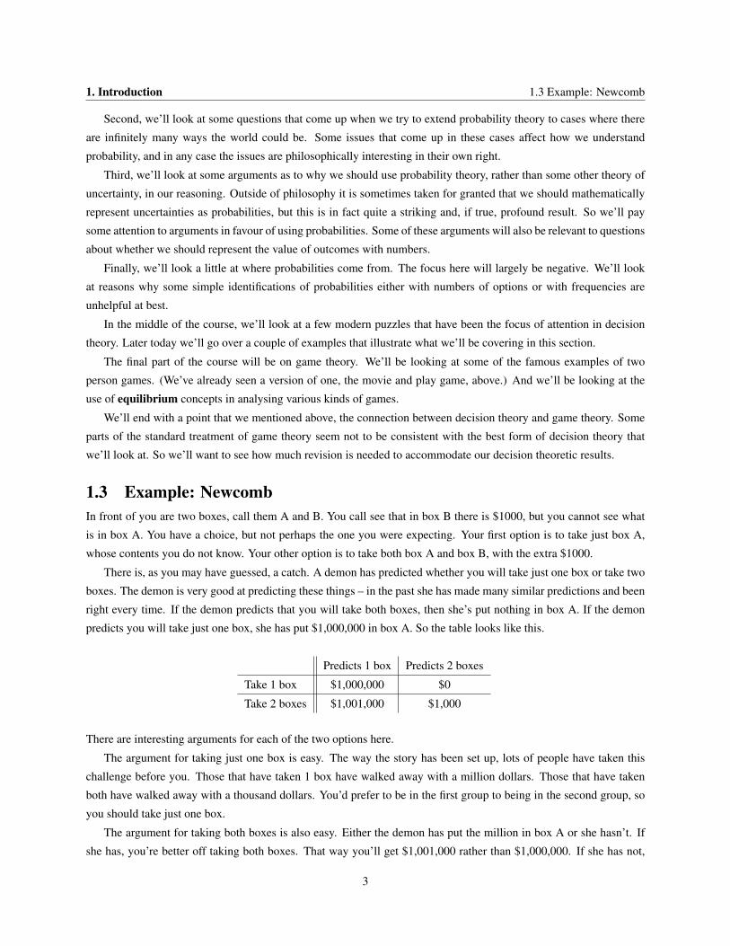
1.3 Example: NewcombIn front of you are two boxes, call them A and B. You call see that in box B there is $1000, but you cannot see what

is in box A. You have a choice, but not perhaps the one you were expecting. Your first option is to take just box A,

whose contents you do not know. Your other option is to take both box A and box B, with the extra $1000.

There is, as you may have guessed, a catch. A demon has predicted whether you will take just one box or take two

boxes. The demon is very good at predicting these things – in the past she has made many similar predictions and been

right every time. If the demon predicts that you will take both boxes, then she’s put nothing in box A. If the demon

predicts you will take just one box, she has put $1,000,000 in box A. So the table looks like this.

Predicts 1 box Predicts 2 boxes

Take 1 box $1,000,000 $0

Take 2 boxes $1,001,000 $1,000

There are interesting arguments for each of the two options here.

The argument for taking just one box is easy. The way the story has been set up, lots of people have taken this

challenge before you. Those that have taken 1 box have walked away with a million dollars. Those that have taken

both have walked away with a thousand dollars. You’d prefer to be in the first group to being in the second group, so

you should take just one box.

The argument for taking both boxes is also easy. Either the demon has put the million in box A or she hasn’t. If

she has, you’re better off taking both boxes. That way you’ll get $1,001,000 rather than $1,000,000. If she has not,

3

1.4 Example: Sleeping Beauty 1. Introduction

you’re better off taking both boxes. That way you’ll get $1,000 rather than $0. Either way, you’re better off taking

both boxes, so you should do that.

Both arguments seem quite strong. The problem is that they lead to incompatible conclusions. So which is correct?

1.4 Example: Sleeping BeautySleeping Beauty is about to undergo a slightly complicated experiment. It is now Sunday night, and a fair coin is about

to be tossed, though Sleeping Beauty won’t see how it lands. Then she will be asked a question, and then she’ll go to

sleep. She’ll be woken up on Monday, asked the same question, and then she’ll go back to sleep, and her memory of

being woken on Monday will be wiped. Then, if (and only if) the coin landed tails, she’ll be woken on Tuesday, and

asked the same question, and then she’ll go back to sleep. Finally, she’ll wake on Wednesday.

The question she’ll be asked is How probable do you think it is that the coin landed heads? What answers

should she give

1. When she is asked on Sunday?

2. When she is asked on Monday?

3. If she is asked on Tuesday?

It seems plausible to suggest that the answers to questions 2 and 3 should be the same. After all, given that

Sleeping Beauty will have forgotten about the Monday waking if she wakes on Tuesday, then she won’t be able to

tell the difference between the Monday and Tuesday waking. So she should give the same answers on Monday and

Tuesday. We’ll assume that in what follows.

First, there seems to be a very good argument for answering 12 to question 1. It’s a fair coin, so it has a probability

of 12 of landing heads. And it has just been tossed, and there hasn’t been any ‘funny business’. So that should be the

answer.

Second, there seems to be a good, if a little complicated, argument for answering 13 to questions 2 and 3. Assume

that questions 2 and 3 are in some sense the same question. And assume that Sleeping Beauty undergoes this experi-

ment many times. Then she’ll be asked the question twice as often when the coin lands tails as when it lands heads.

That’s because when it lands tails, she’ll be asked that question twice, but only once when it lands heads. So only 13 of

the time when she’s asked this question, will it be true that the coin landed heads. And plausibly, if you’re going to be

repeatedly asked How probable is it that such-and-such happened, and 13 of the time when you’re asked that question,

such-and-such will have happened, then you should answer 13 each time.

Finally, there seems to be a good argument for answering questions 1 and 2 the same way. After all, Sleeping

Beauty doesn’t learn anything new between the two questions. She wakes up, but she knew she was going to wake

up. And she’s asked the question, but she knew she was going to be asked the question. And it seems like a decent

principle that if nothing happens between Sunday and Monday to give you new evidence about a proposition, the

probability that you think it did happen shouldn’t change.

But of course, these three arguments can’t all be correct. So we have to decide which one is incorrect.

Upcoming These are just two of the puzzles we’ll be looking at as the course proceeds. Some of these will be decision

puzzles, like Newcomb’s Problem. Some of them will be probability puzzles that are related to decision theory, like

Sleeping Beauty. And some will be game puzzles. I hope the puzzles are somewhat interesting. I hope even more that

we learn something from them.

4

Chapter 2 Simple Reasoning Strategies

2.1 Dominance ReasoningThe simplest rule we can use for decision making is never choose dominated options. There is a stronger and a weaker

version of this rule.

An option A strongly dominated another option B if in every state, A leads to better outcomes than B. A weaklydominates B if in every state, A leads to at least as good an outcome as B, and in some states it leads to better

outcomes.

We can use each of these as decision principles. The dominance principle we’ll be primarily interested in says

that if A strongly dominates B, then A should be preferred to B. We get a slightly stronger principle if we use weak

dominance. That is, we get a slightly stronger principle if we say that whenever A weakly dominates B, A should be

chosen over B. It’s a stronger principle because it applies in more cases — that is, whenever A strongly dominates B,

it also weakly dominates B.

Dominance principles seem very intuitive when applied to everyday decision cases. Consider, for example, a

revised version of our case about choosing whether to watch football or work on a term paper. Imagine that you’ll do

very badly on the term paper if you leave it to the last minute. And imagine that the term paper is vitally important for

something that matters to your future. Then we might set up the decision table as follows.

Your team wins Your team loses

Watch football 2 1

Work on paper 4 3

If your team wins, you are better off working on the paper, since 4 > 2. And if your team loses, you are better off

working on the paper, since 3 > 1. So either way you are better off working on the paper. So you should work on the

paper.

2.2 States and ChoicesHere is an example from Jim Joyce that suggests that dominance might not be as straightforward a rule as we suggested

above.

Suupose you have just parked in a seedy neighborhood when a man approaches and offers to “protect”

your car from harm for $10. You recognize this as extortion and have heard that people who refuse

“protection” invariably return to find their windshields smashed. Those who pay find their cars intact.

You cannot park anywhere else because you are late for an important meeting. It costs $400 to replace

a windshield. Should you buy “protection”? Dominance says that you should not. Since you would

5

2.3 Maximin and Maximax 2. Simple Reasoning Strategies

rather have the extra $10 both in the even that your windshield is smashed and in the event that it is not,

Dominance tells you not to pay. (Joyce, The Foundations of Causal Decision Theory, pp 115-6.)

We can put this in a table to make the dominance argument that Joyce suggests clearer.

Broken Windshield Unbroken Windshield

Pay extortion -$410 -$10

Don’t pay -$400 0

In each column, the number in the ‘Don’t pay’ row is higher than the number in the ‘Pay extortion’ row. So it looks

just like the case above where we said dominance gives a clear answer about what to do. But the conclusion is crazy.

Here is how Joyce explains what goes wrong in the dominance argument.

Of course, this is absurd. Your choice has a direct influence on the state of the world; refusing to pay

makes it likly that your windshield will be smashed while paying makes this unlikely. The extortionist is

a despicable person, but he has you over a barrel and investing a mere $10 now saves $400 down the line.

You should pay now (and alert the police later).

This seems like a general principle we should endorse. We should define states as being, intuitively, independent

of choices. The idea behind the tables we’ve been using is that the outcome should depend on two factors - what you

do and what the world does. If the ‘states’ are dependent on what choice you make, then we won’t have successfully

‘factorised’ the dependence of outcomes into these two components.

We’ve used a very intuitive notion of ‘independence’ here, and we’ll have a lot more to say about that in later

sections. It turns out that there are a lot of ways to think about independence, and they yield different recommendations

about what to do. For now, we’ll try to use ‘states’ that are clearly independent of the choices we make.

2.3 Maximin and MaximaxDominance is a (relatively) uncontroversial rule, but it doesn’t cover a lot of cases. We’ll start now lookintg at rules

that are more or less comprehensive. To start off, let’s consider rules that we might consider rules for optimists and

pessimists respectively.

The Maximax rule says that you should maximise the maximum outcome you can get. Basically, consider the

best possible outcome, consider what you’d have to do to bring that about, and do it. In general, this isn’t a very

plausible rule. It recommends taking any kind of gamble that you are offered. If you took this rule to Wall St, it would

recommend buying the riskiest derivatives you could find, because they might turn out to have the best results. Perhaps

needless to say, I don’t recommend that strategy.

The Maximin rule says that you should maximise the minimum outcome you can get. So for every choice, you

look at the worst-case scenario for that choice. You then pick the option that has the least bad worst case scenario.

Consider the following list of preferences from our watch football/work on paper example.


Watch football 4 1

Work on paper 3 2

6

2. Simple Reasoning Strategies 2.4 Ordinal and Cardinal Utilities

So you’d prefer your team to win, and you’d prefer to watch if they win, and work if they lose. So the worst case

scenario if you watch the game is that they lose - the worst case scenario of all in the game. But the worst case scenario

if you don’t watch is also that they lose. Still that wasn’t as bad as watching the game and seeing them lose. So you

should work on the paper.

We can change the example a little without changing the recommendation.


Watch football 4 1

Work on paper 2 3

In this example, your regret at missing the game overrides your desire for your team to win. So if you don’t watch,

you’d prefer that they lose. Still the worst case scenario is you don’t watch is 2, and the worst case scenario if you do

watch is 1. So, according to maximin, you should not watch.

Note in this case that the worst case scenario is a different state for different choices. Maximin doesn’t require that

you pick some ‘absolute’ worst-case scenario and decide on the assumption it is going to happen. Rather, you look at

different worst case scenarios for different choices, and compare them.

2.4 Ordinal and Cardinal UtilitiesAll of the rules we’ve looked at so far depend only on the ranking of various options. They don’t depend on how much

we prefer one option over another. They just depend on which order we rank goods is.

To use the technical language, so far we’ve just looked at rules that just rely on ordinal utilities. The term ordinal

here means that we only look at the order of the options. The rules that we’ll look at rely on cardinal utilities.

Whenever we’re associating outcomes with numbers in a way that the magnitudes of the differences between the

numbers matters, we’re using cardinal utilities.

It is rather intuitive that something more than the ordering of outcomes should matter to what decisions we make.

Imagine that two agents, Chris and Robin, each have to make a decision between two airlines to fly them from New

York to San Francisco. One airline is more expensive, the other is more reliable. To oversimplify things, let’s say

the unreliable airline runs well in good weather, but in bad weather, things go wrong. And Chris and Robin have no

way of finding out what the weather along the way will be. They would prefer to save money, but they’d certainly not

prefer for things to go badly wrong. So they face the following decision table.

Good weather Bad weather

Fly cheap airline 4 1

Fly good airline 3 2

If we’re just looking at the ordering of outcomes, that is the decision problem facing both Chris and Robin.

But now let’s fill in some more details about the cheap airlines they could fly. The cheap airline that Chris might

fly has a problem with luggage. If the weather is bad, their passengers’ luggage will be a day late getting to San

Francisco. The cheap airline that Robin might fly has a problem with staying in the air. If the weather is bad, their

plane will crash.

7

2.5 Regret 2. Simple Reasoning Strategies

Those seem like very different decision problems. It might be worth risking one’s luggage being a day late in order

to get a cheap plane ticket. It’s not worth risking, seriously risking, a plane crash. (Of course, we all take some risk of

being in a plane crash, unless we only ever fly the most reliable airline that we possibly could.) That’s to say, Chris and

Robin are facing very different decision problems, even though the ranking of the four possible outcomes is the same

in each of their cases. So it seems like some decision rules should be sensitive to magnitudes of differences between

options. The first kind of rule we’ll look at uses the notion of regret.

2.5 RegretWhenever you are faced with a decision problem without a dominating option, there is a chance that you’ll end up

taking an option that turns out to be sub-optimal. If that happens there is a chance that you’ll regret the choice you take.

That isn’t always the case. Sometimes you decide that you’re happy with the choice you made after all. Sometimes

you’re in no position to regret what you chose because the combination of your choice and the world leaves you dead.

Despite these complications, we’ll define the regret of a choice to be the difference between the value of the best

choice given that state, and the value of the choice in question. So imagine that you have a choice between going to

the movies, going on a picnic or going to a baseball game. And the world might produce a sunny day, a light rain day,

or a thunderstorm. We might imagine that your values for the nine possible choice-world combinations are as follows.

Sunny Light rain Thunderstorm

Picnic 20 5 0

Baseball 15 2 6

Movies 8 10 9

Then the amount of regret associated with each choice, in each state, is as follows


Picnic 0 5 9

Baseball 5 8 3

Movies 12 0 0

Look at the middle cell in the table, the 8 in the baseball row and light rain column. The reason that’s a 8 is that in that

possibility, you get utility 2. But you could have got utility 10 from going to the movies. So the regret level is 10 - 2,

that is, 8.

There are a few rules that we can describe using the notion of regret. The most commonly discussed one is called

Minimax regret. The idea behind this rule is that you look at what the maximum possible regret is for each option. So

in the above example, the picnic could end up with a regret of 9, the baseball with a regret of 8, and the movies with a

regret of 12. Then you pick the option with the lowest maximum possible regret. In this case, that’s the baseball.

The minimax regret rule leads to plausible outcomes in a lot of cases. But it has one odd structural property. In

this case it recommends choosing the baseball over the movies and picnic. Indeed, it thinks going to the movies is the

worst option of all. But now imagine that the picnic is ruled out as an option. (Perhaps we find out that we don’t have

any way to get picnic food.) Then we have the following table.

8

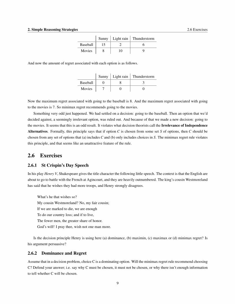
2. Simple Reasoning Strategies 2.6 Exercises


Baseball 15 2 6

Movies 8 10 9

And now the amount of regret associated with each option is as follows.


Baseball 0 8 3

Movies 7 0 0

Now the maximum regret associated with going to the baseball is 8. And the maximum regret associated with going

to the movies is 7. So minimax regret recommends going to the movies.

Something very odd just happened. We had settled on a decision: going to the baseball. Then an option that we’d

decided against, a seemingly irrelevant option, was ruled out. And because of that we made a new decision: going to

the movies. It seems that this is an odd result. It violates what decision theorists call the Irrelevance of IndependenceAlternatives. Formally, this principle says that if option C is chosen from some set S of options, then C should be

chosen from any set of options that (a) includes C and (b) only includes choices in S. The minimax regret rule violates

this principle, and that seems like an unattractive feature of the rule.

2.6 Exercises

2.6.1 St Crispin’s Day Speech

In his play Henry V, Shakespeare gives the title character the following little speech. The context is that the English are

about to go to battle with the French at Agincourt, and they are heavily outnumbered. The king’s cousin Westmoreland

has said that he wishes they had more troops, and Henry strongly disagrees.

What’s he that wishes so?

My cousin Westmoreland? No, my fair cousin;

If we are marked to die, we are enough

To do our country loss; and if to live,

The fewer men, the greater share of honor.

God’s will! I pray thee, wish not one man more.

Is the decision principle Henry is using here (a) dominance, (b) maximin, (c) maximax or (d) minimax regret? Is

his argument persuasive?

2.6.2 Dominance and Regret

Assume that in a decision problem, choice C is a dominating option. Will the minimax regret rule recommend choosing

C? Defend your answer; i.e. say why C must be chosen, it must not be chosen, or why there isn’t enough information

to tell whether C will be chosen.

9

2.6 Exercises 2. Simple Reasoning Strategies

2.6.3 Irrelevance of Independent Alternatives

Sam always chooses by the maximax rule. Will Sam’s choices satisfy the irrelevance of independent alternatives

condition? Say why or why not.

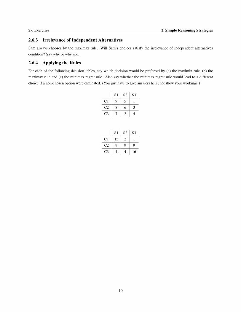
2.6.4 Applying the Rules

For each of the following decision tables, say which decision would be preferred by (a) the maximin rule, (b) the

maximax rule and (c) the minimax regret rule. Also say whether the minimax regret rule would lead to a different

choice if a non-chosen option were elminated. (You just have to give answers here, not show your workings.)

S1 S2 S3

C1 9 5 1

C2 8 6 3

C3 7 2 4

S1 S2 S3

C1 15 2 1

C2 9 9 9

C3 4 4 16

10

Chapter 3 Uncertainty

3.1 Likely OutcomesEarlier we considered the a decision problem, basically deciding what to do with a Sunday afternoon, that had the

following table.


Picnic 20 5 0

Baseball 15 2 6

Movies 8 10 9

We looked at how a few different decision rules would treat this decision. The maximin rule would recommend going

to the movies, the maximax rule going to the picnic, and the minimax regret rule going to the baseball.

But if we were faced with that kind of decision in real life, we wouldn’t sit down to start thinking about which of

those three rules were correct, and using the answer to that philosophical question to determine what to do. Rather,

we’d consult a weather forecast. If it looked like it was going to be sunny, we’d go on a picnic. If it looked like it was

going to rain, we’d go to the movie. What’s relevant is how likely each of the three states of the world are. That’s

something none of our decision rules to date have considered, and it seems like a large omission.

In general, how likely various states are plays a major role in deciding what to do. Consider the following broad

kind of decision problem. There is a particular disease that, if you catch it and don’t have any drugs to treat it with, is

likely fatal. Buying the drugs in question will cost $500. Do you buy the drugs?

Well, that probably depends on how likely it is that you’ll catch the disease in the first place. The case isn’t entirely

hypothetical. You or I could, at this moment, be stockpiling drugs that treat anthrax poisoning, or avian flu. I’m not

buying drugs to defend against either thing. If it looked more likely that there would be more terrorist attacks using

anthrax, or an avian flu epidemic, then it would be sensible to spend $500, and perhaps a lot more, defending against

them. As it stands, that doesn’t seem particularly sensible. (I have no idea exactly how much buying the relevant drugs

would cost; the $500 figure was somewhat made up. I suspect it would be a rolling cost because the drugs would go

‘stale’.)

We’ll start off today looking at various decision rules that might be employed taking account of the likelihood

of various outcomes. Then we’ll look at what we might mean by likelihoods. This will start us down the track to

discussions of probability, a subject that we’ll be interested in for most of the rest of the course.

3.2 Do What’s Likely to WorkThe following decision rule doesn’t have a catchy name, but I’ll call it Do What’s Likely to Work. The idea is that we

should look at the various states that could come about, and decide which of them is most likely to actually happen.

11

3.2 Do What’s Likely to Work 3. Uncertainty

This is more or less what we would do in the decision above about what to do with a Sunday afternoon. The rule says

then we should make the choice that will result in the best outcome in that most likely of states.

The rule has two nice advantages. First, it doesn’t require a very sophisticated theory of likelihoods. It just requires

us to be able to rank the various states in terms of how likely they are. Using some language from the previous section,

we rely on a ordinarl rather than a cardinal theory of likelihoods. Second, it matches up well enough with a lot of our

everyday decisions. In real life cases like the above example, we really do decide what state is likely to be actual (i.e.

decide what the weather is likely to be) then decide what would be best to do in that circumstance.

But the rule also leads to implausible recommendations in other real life cases. Indeed, in some cases it is so

implausible that it seems that it must at some level be deeply mistaken. Here is a simple example of such a case.

You have been exposed to a deadly virus. About 13 of people who are exposed to the virus are infected by it, and

all those infected by it die unless they receive a vaccine. By the time any symptoms of the virus show up, it is too late

for the vaccine to work. You are offered a vaccine for $500. Do you take it or not?

Well, the most likely state of the world is that you don’t have the virus. After all, only 13 of people who are exposed

catch the virus. The other 23 do not, and the odds are that you are in that group. And if you don’t have the virus, it isn’t

worth paying $500 for a vaccine against a virus you haven’t caught. So by “Do What’s Likely to Work”, you should

decline the vaccine.

But that’s crazy! It seems as clear as anything that you should pay for the vaccine. You’re in serious danger of

dying here, and getting rid of that risk for $500 seems like a good deal. So “Do What’s Likely to Work” gives you the

wrong result. There’s a reason for this. You stand to lose a lot if you die. And while $500 is a lot of money, it’s a lot

less of a loss than dying. Whenever the downside is very different depending on which choice you make, sometimes

you should avoid the bigger loss, rather than doing the thing that is most likely to lead to the right result.

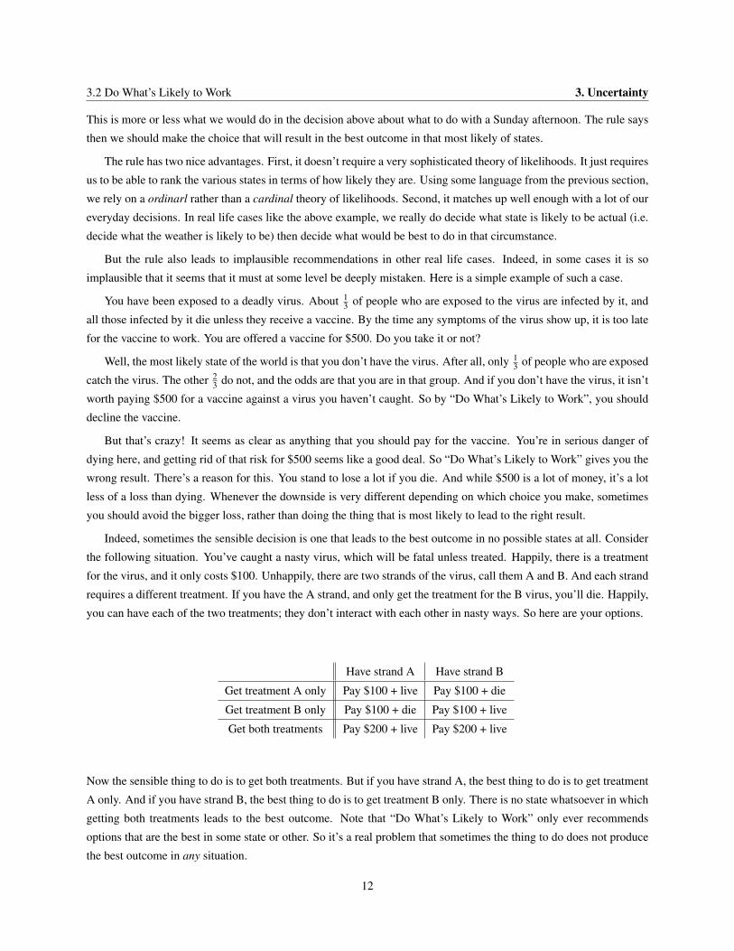
Indeed, sometimes the sensible decision is one that leads to the best outcome in no possible states at all. Consider

the following situation. You’ve caught a nasty virus, which will be fatal unless treated. Happily, there is a treatment

for the virus, and it only costs $100. Unhappily, there are two strands of the virus, call them A and B. And each strand

requires a different treatment. If you have the A strand, and only get the treatment for the B virus, you’ll die. Happily,

you can have each of the two treatments; they don’t interact with each other in nasty ways. So here are your options.

Have strand A Have strand B

Get treatment A only Pay $100 + live Pay $100 + die

Get treatment B only Pay $100 + die Pay $100 + live

Get both treatments Pay $200 + live Pay $200 + live

Now the sensible thing to do is to get both treatments. But if you have strand A, the best thing to do is to get treatment

A only. And if you have strand B, the best thing to do is to get treatment B only. There is no state whatsoever in which

getting both treatments leads to the best outcome. Note that “Do What’s Likely to Work” only ever recommends

options that are the best in some state or other. So it’s a real problem that sometimes the thing to do does not produce

the best outcome in any situation.

12

3. Uncertainty 3.3 Probability and Uncertainty

3.3 Probability and UncertaintyAs I mentioned above, none of the rules we’d looked at before today took into account the likelihood of the various

states of the world. Some authors have been tempted to see this as a feature not a bug. To see why, we need to look at

a common three-fold distinction between states.

There are lots of things we know, even that we’re certain about. If we are certain which state of the world will be

actual, call the decision we face a decision under certainty.

Some times we don’t know which state will be actual. But we can state precisely what the probability is that each

of the states in question will be actual. For instance, if we’re trying to decide whether to bet on a roulette wheel, then

the relevant states will be the 37 or 38 slots in which the ball can land. We can’t know which of those will happen,

but we do know the probability of each possible state. In cases where we can state the relevant probabilities, call the

decision we face a decision under risk.

In other cases, we can’t even state any probabilities. Imagine the following (not entirely unrealistic) case. You

have an option to invest in a speculative mining venture. The people doing the projections for the investment say that

it will be a profitable investment, over its lifetime, if private cars running primarily on fossil fuel products are still the

dominant form of transportation in 20 years time. Maybe that will happen, maybe it won’t. It depends a lot on how

non fossil-fuel energy projects go, and I gather that that’s very hard to predict. Call such a decision, one where we

can’t even assign probabilities to states, a Decision under uncertainty.

It is sometimes proposed that rules like maximin, and minimax regret, while they are clearly bad rules to use for

decisions under risk, might be good rules for decisions under uncertainty. I suspect that isn’t correct, largely because

I suspect the distinction between decisions under risk and decisions under uncertainty is not as sharp as the above

tripartite distinction suggests. Here is a famous passage from John Maynard Keynes, written in 1937, describing the

distinction between risk and uncertainty.

By “uncertain” knowledge, let me explain, I do not mean merely to distinguish what is known for certain

from what is only probable. The game of roulette is not subject, in this sense, to uncertainty; nor is the

prospect of a Victory bond being drawn. Or, again, the expectation of life is only slightly uncertain. Even

the weather is only moderately uncertain. The sense in which I am using the term is that in which the

prospect of a European war is uncertain, or the price of copper and the rate of interest twenty years hence,

or the obsolescence of a new invention, or the position of private wealth owners in the social system

in 1970. About these matters there is no scientific basis on which to form any calculable probability

whatever. We simply do not know. Nevertheless, the necessity for action and for decision compels us as

practical men to do our best to overlook this awkward fact and to behave exactly as we should if we had

behind us a good Benthamite calculation of a series of prospective advantages and disadvantages, each

multiplied by its appropriate probability, waiting to be summed.

There’s something very important about how Keynes sets up the distinction between risk and uncertainty here. He

says that it is a matter of degree. Some things are very uncertain, such as the position of wealth holders in the social

system a generation hence. Some things are a little uncertain, such as the weather in a week’s time. We need a way of

thinking about risk and uncertainty that allows that in many cases, we can’t say exactly what the relevant probabilities

are, but we can say something about the comparative likelihoods.

13

3.3 Probability and Uncertainty 3. Uncertainty

Let’s look more closely at the case of the weather. In particular, think about decisions that you have to make which

turn on what the weather will be like in 7 to 10 days time. These are a particularly tricky range of cases to think about.

If your decision turns on what the weather will be like in the distant future, you can look at historical data. That

data might not tell you much about the particular day you’re interested in, but it will be reasonably helpful in setting

probabilities. For instance, if it has historically rained on 17% of August days in your hometown, then it isn’t utterly

crazy to think the probability it will rain on August 19 in 3 years time is about 0.17.

If your decision turns on what the weather will be like in the near future, such as the next few hours or days, you

have a lot of information ready to hand on which to base a decision. Looking out the window is a decent guide to what

the weather will be like for the next hour, and looking up a professional weather service is a decent guide to what it

will be for days after that.

But in between those two it is hard. What do you think if historically it rarely rains at this time of year, but the

forecasters think there’s a chance a storm is brewing out west that could arrive in 7 to 10 days? It’s hard even to assign

probabilities to whether it will rain.

But this doesn’t mean that we should throw out all information we have about relative likelihoods. I don’t know

what the weather will be like in 10 days time, and I can’t even sensibly assign probabilities to outcomes, but I’m not in

a state of complete uncertainty. I have a little information, and that information is useful in making decisions. Imagine

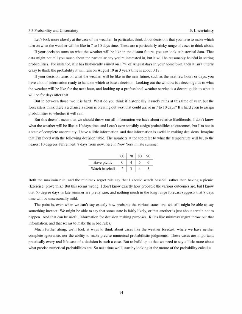
that I’m faced with the following decision table. The numbers at the top refer to what the temperature will be, to the

nearest 10 degrees Fahrenheit, 8 days from now, here in New York in late summer.

60 70 80 90

Have picnic 0 4 5 6

Watch baseball 2 3 4 5

Both the maximin rule, and the minimax regret rule say that I should watch baseball rather than having a picnic.

(Exercise: prove this.) But this seems wrong. I don’t know exactly how probable the various outcomes are, but I know

that 60 degree days in late summer are pretty rare, and nothing much in the long range forecast suggests that 8 days

time will be unseasonally mild.

The point is, even when we can’t say exactly how probable the various states are, we still might be able to say

something inexact. We might be able to say that some state is fairly likely, or that another is just about certain not to

happen. And that can be useful information for decision making purposes. Rules like minimax regret throw out that

information, and that seems to make them bad rules.

Much further along, we’ll look at ways to think about cases like the weather forecast, where we have neither

complete ignorance, nor the ability to make precise numerical probabilistic judgments. These cases are important;

practically every real-life case of a decision is such a case. But to build up to that we need to say a little more about

what precise numerical probabilities are. So next time we’ll start by looking at the nature of the probability calculus.

14

Chapter 4 Measures

4.1 Probability DefinedWe talk informally about probabilities all the time. We might say that it is more probable than not that such-and-such

team will make the playoffs. Or we might say that it’s very probable that a particular defendant will be convicted at

his trial. Or that it isn’t very probable that the next card will be the one we need to complete this royal flush.

We also talk formally about probability in mathematical contexts. Formally, a probability function is a normalised

measure over a possibility space. Below we’ll be saying a fair bit about what each of those terms mean. We’ll start with

measure, then say what a normalised measure is, and finally (over the next two days) say something about possibility

spaces.

There is a very important philosophical question about the connection between our informal talk and our formal

talk. In particular, it is a very deep question whether this particular kind of formal model is the right model to

represent our informal, intuitive concept. The vast majority of philosophers, statisticians, economists and others who

work on these topics think it is, though as always there are dissenters. We’ll be spending a fair bit of time later in this

course on this philosophical question. But before we can even answer that question we need to understand what the

mathematicians are talking about when they talk about probabilities. And that requires starting with the notion of a

measure.

4.2 MeasuresA measure is a function from ‘regions’ of some space to non-negative numbers with the following property. If A is a

region that divides exactly into regions B and C, then the measure of A is the sum of the measures of B and C. And

more generally, if A divides exactly into regions B1, B2, ..., Bn, then the measure of A will be the sum of the measures

of B1, B2, ... and Bn.

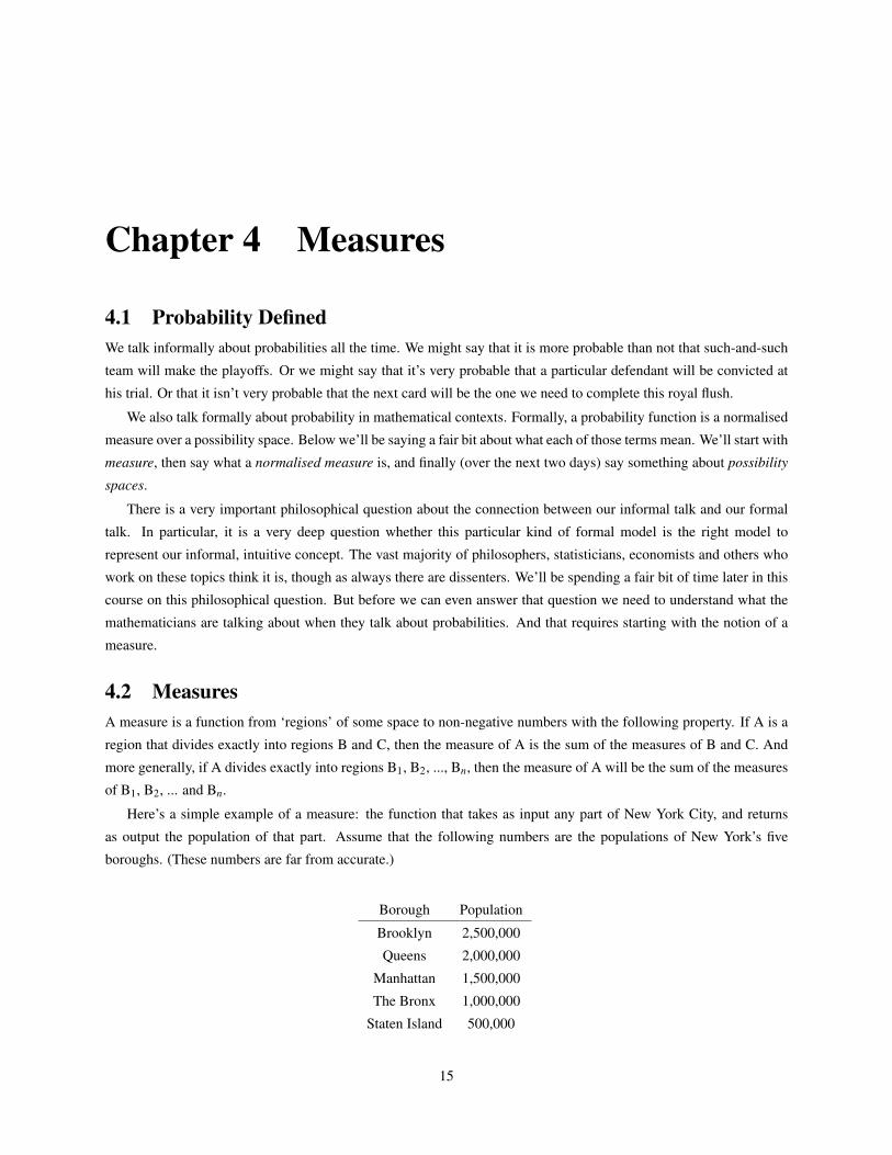
Here’s a simple example of a measure: the function that takes as input any part of New York City, and returns

as output the population of that part. Assume that the following numbers are the populations of New York’s five

boroughs. (These numbers are far from accurate.)

Borough Population

Brooklyn 2,500,000

Queens 2,000,000

Manhattan 1,500,000

The Bronx 1,000,000

Staten Island 500,000

15

4.2 Measures 4. Measures

We can already think of this as a function, with the left hand column giving the inputs, and the right hand column

the values. Now if this function is a measure, it should be additive in the sense described above. So consider the part

of New York City that’s on Long Island. That’s just Brooklyn plus Queens. If the population function is a measure,

the value of that function, as applied to the Long Island part of New York, should be 2,500,000 plus 2,000,000, i.e.

4,500,000. And that makes sense: the population of Brooklyn plus Queens just is the population of Brooklyn plus the

population of Queens.

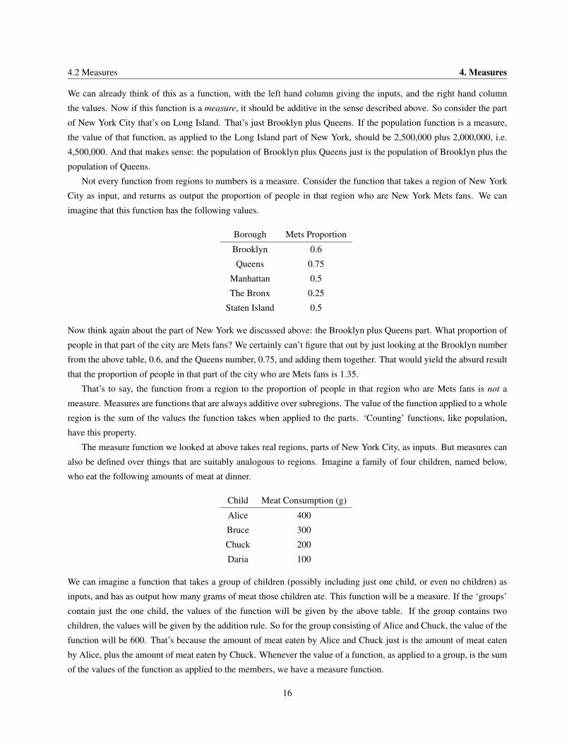
Not every function from regions to numbers is a measure. Consider the function that takes a region of New York

City as input, and returns as output the proportion of people in that region who are New York Mets fans. We can

imagine that this function has the following values.

Borough Mets Proportion

Brooklyn 0.6

Queens 0.75

Manhattan 0.5

The Bronx 0.25

Staten Island 0.5

Now think again about the part of New York we discussed above: the Brooklyn plus Queens part. What proportion of

people in that part of the city are Mets fans? We certainly can’t figure that out by just looking at the Brooklyn number

from the above table, 0.6, and the Queens number, 0.75, and adding them together. That would yield the absurd result

that the proportion of people in that part of the city who are Mets fans is 1.35.

That’s to say, the function from a region to the proportion of people in that region who are Mets fans is not a

measure. Measures are functions that are always additive over subregions. The value of the function applied to a whole

region is the sum of the values the function takes when applied to the parts. ‘Counting’ functions, like population,

have this property.

The measure function we looked at above takes real regions, parts of New York City, as inputs. But measures can

also be defined over things that are suitably analogous to regions. Imagine a family of four children, named below,

who eat the following amounts of meat at dinner.

Child Meat Consumption (g)

Alice 400

Bruce 300

Chuck 200

Daria 100

We can imagine a function that takes a group of children (possibly including just one child, or even no children) as

inputs, and has as output how many grams of meat those children ate. This function will be a measure. If the ‘groups’

contain just the one child, the values of the function will be given by the above table. If the group contains two

children, the values will be given by the addition rule. So for the group consisting of Alice and Chuck, the value of the

function will be 600. That’s because the amount of meat eaten by Alice and Chuck just is the amount of meat eaten

by Alice, plus the amount of meat eaten by Chuck. Whenever the value of a function, as applied to a group, is the sum

of the values of the function as applied to the members, we have a measure function.

16

4. Measures 4.3 Normalised Measures

4.3 Normalised MeasuresA measure function is defined over some regions. Usually one of those regions will be the ‘universe’ of the function;

that is, the region made up of all those regions the function is defined over. In the case where the regions are regions

of physical space, as in our New York example, that will just be the physical space consisting of all the smaller regions

that are inputs to the function. In our New York example, the universe is just New York City. In cases where the

regions are somewhat more metaphorical, as in the case of the children’s meat-eating, the universe will also be defined

somewhat more metaphorically. In that case, it is just the group consisting of the four children.

However the universe is defined, a normalised measure is simply a measure function where the value the function

gives to the universe is 1. So for every sub-region of the universe, its measure can be understood as a proportion of the

universe.

We can ‘normalise’ any measure by simply dividing each value through by the value of the universe. If we wanted

to normalise our New York City population measure, we would simply divide all values by 7,500,000. The values we

would then end up with are as follows.

Borough Population

Brooklyn 13

Queens 415

Manhattan 15

The Bronx 215

Staten Island 13

Some measures may not have a well-defined universe, and in those cases we cannot normalise the measure. But

generally normalisation is a simple matter of dividing everything by the value the function takes when applied to the

whole universe. And the benefit of doing this is that it gives us a simple way of representing proportions.

4.4 FormalitiesSo far I’ve given a fairly informal description of what measures are, and what normalised measures are. In this section

we’re going to go over the details more formally. If you understand the concepts well enough already, or if you aren’t

familiar enough with set theory to follow this section entirely, you should feel free to skip forward to the next section.

Note that this is a slightly simplified, and hence slightly inaccurate, presentation; we aren’t focussing on issues to do

with infinity. Those will be covered later in the course.

A measure is a function m satisfying the following conditions.

1. The domain D is a set of sets.

2. The domain is closed under union, intersection and complementation with respect to the relevant universe U.

That is, if A ∈ D and B ∈ D, then (A∪B) ∈ D and (A∪B) ∈ D and U \A ∈ D

3. The range is a set of non-negative real numbers

4. The function is additive in the following sense: If A∩B = /0, then m(A∪B) = m(A)+m(B)

We can prove some important general results about measures using just these properties. Note that we the following

results follow more or less immediately from additivity.

17

4.5 Possibility Space 4. Measures

1. m(A) = m(A∩B)+m(A∩ (U \B))

2. m(B) = m(A∩B)+m(B∩ (U \A))

3. m(A∪B) = m(A∩B)+m(A∩ (U \B))+m(B∩ (U \A))

The first says that the measure of A is the measure of A’s intersection with B, plus the measure of A’s intersection

with the complement of B. The first says that the measure of B is the measure of A’s intersection with B, plus the

measure of B’s intersection with the complement of A. In each case the point is that a set is just made up of its

intersection with some other set, plus its intersection with the complement of that set. The final line relies on the fact

that the union of A and B is made up of (i) their intersection, (ii) the part of A that overlaps B’s complement and (iii)

the part of B that overlaps A’s complement. So the measure of A∪B should be the sum of the measure of those three

sets.

Note that if we add up the LHS and RHS of lines 1 and 2 above, we get

m(A)+m(B) = m(A∩B)+m(A∩ (U \B))+m(A∩B)+m(A∩ (U \B))

And subtracting m(A∩B) from each side, we get

m(A)+m(B)−m(A∩B) = m(A∩B)+m(A∩ (U \B))+m(A∩ (U \B))

But that equation, plus line 3 above, entails that

m(A)+m(B)−m(A∩B) = m(A∪B)

And that identity holds whether or not A∩B is empty. If A∩B is empty, the result is just equivalent to the addition

postulate, but in general it is a stronger result, and one we’ll be using a fair bit in what follows.

4.5 Possibility SpaceImagine you’re watching a baseball game. There are lots of ways we could get to the final result, but there are just

two ways the game could win. The home team could win, call this possibility H, or the away team could win, call this

possibility A.

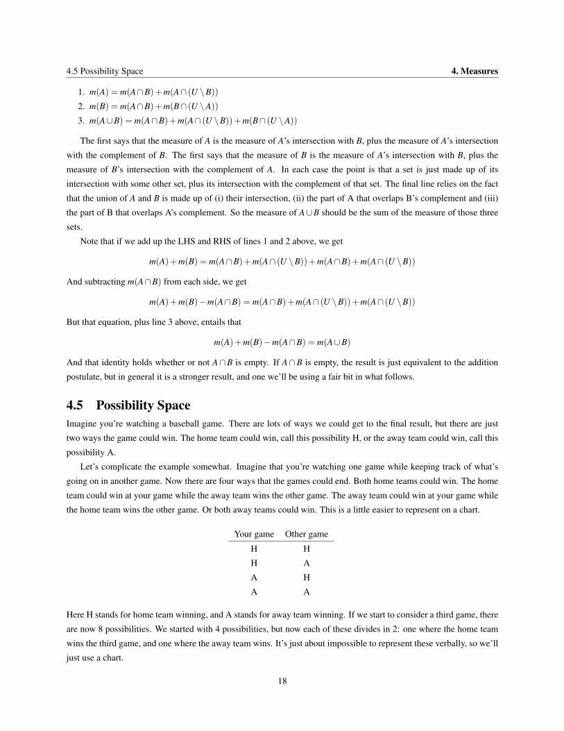
Let’s complicate the example somewhat. Imagine that you’re watching one game while keeping track of what’s

going on in another game. Now there are four ways that the games could end. Both home teams could win. The home

team could win at your game while the away team wins the other game. The away team could win at your game while

the home team wins the other game. Or both away teams could win. This is a little easier to represent on a chart.

Your game Other game

H H

H A

A H

A A

Here H stands for home team winning, and A stands for away team winning. If we start to consider a third game, there

are now 8 possibilities. We started with 4 possibilities, but now each of these divides in 2: one where the home team

wins the third game, and one where the away team wins. It’s just about impossible to represent these verbally, so we’ll

just use a chart.

18

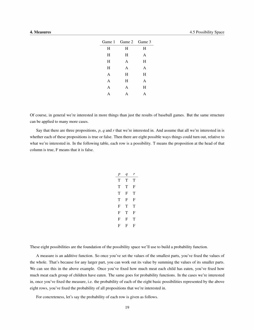
4. Measures 4.5 Possibility Space

Game 1 Game 2 Game 3

H H H

H H A

H A H

H A A

A H H

A H A

A A H

A A A

Of course, in general we’re interested in more things than just the results of baseball games. But the same structure

can be applied to many more cases.

Say that there are three propositions, p, q and r that we’re interested in. And assume that all we’re interested in is

whether each of these propositions is true or false. Then there are eight possible ways things could turn out, relative to

what we’re interested in. In the following table, each row is a possibility. T means the proposition at the head of that

column is true, F means that it is false.

p q r

T T T

T T F

T F T

T F F

F T T

F T F

F F T

F F F

These eight possibilities are the foundation of the possibility space we’ll use to build a probability function.

A measure is an additive function. So once you’ve set the values of the smallest parts, you’ve fixed the values of

the whole. That’s because for any larger part, you can work out its value by summing the values of its smaller parts.

We can see this in the above example. Once you’ve fixed how much meat each child has eaten, you’ve fixed how

much meat each group of children have eaten. The same goes for probability functions. In the cases we’re interested

in, once you’ve fixed the measure, i.e. the probability of each of the eight basic possibilities represented by the above

eight rows, you’ve fixed the probability of all propositions that we’re interested in.

For concreteness, let’s say the probability of each row is given as follows.

19

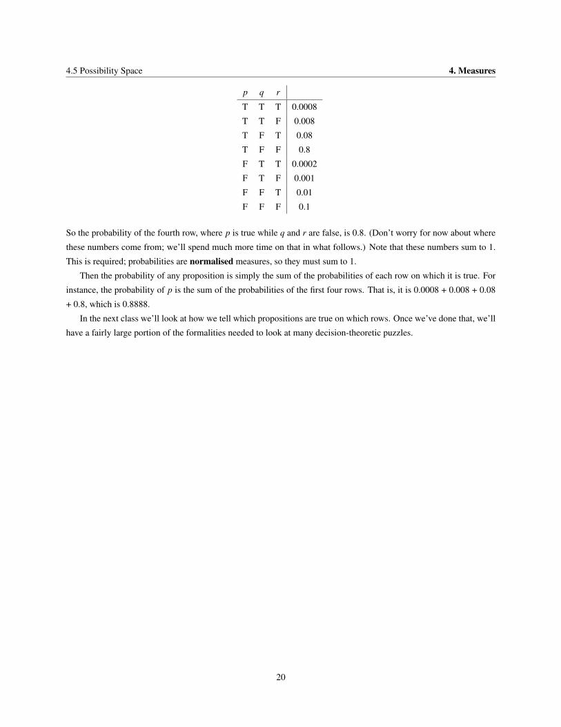
4.5 Possibility Space 4. Measures

p q r

T T T 0.0008

T T F 0.008

T F T 0.08

T F F 0.8

F T T 0.0002

F T F 0.001

F F T 0.01

F F F 0.1

So the probability of the fourth row, where p is true while q and r are false, is 0.8. (Don’t worry for now about where

these numbers come from; we’ll spend much more time on that in what follows.) Note that these numbers sum to 1.

This is required; probabilities are normalised measures, so they must sum to 1.

Then the probability of any proposition is simply the sum of the probabilities of each row on which it is true. For

instance, the probability of p is the sum of the probabilities of the first four rows. That is, it is 0.0008 + 0.008 + 0.08

+ 0.8, which is 0.8888.

In the next class we’ll look at how we tell which propositions are true on which rows. Once we’ve done that, we’ll

have a fairly large portion of the formalities needed to look at many decision-theoretic puzzles.

20

Chapter 5 Truth Tables

5.1 Compound SentencesSome sentences have other sentences as parts. We’re going to be especially interested in sentences that have the

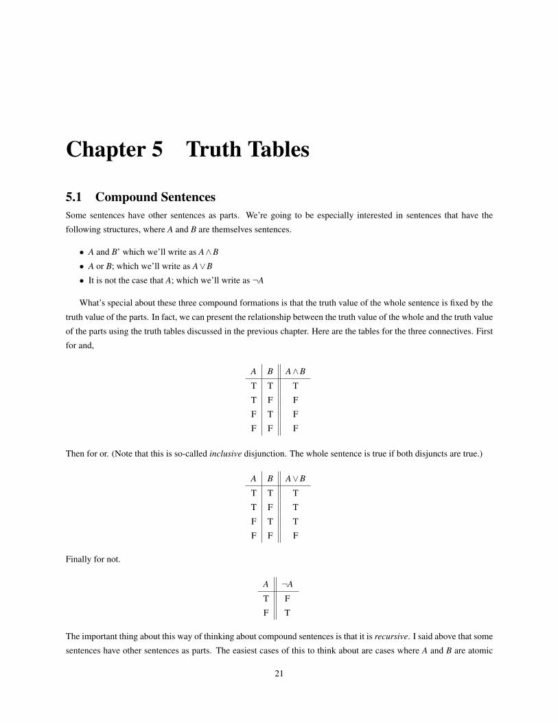
following structures, where A and B are themselves sentences.

• A and B’ which we’ll write as A∧B

• A or B; which we’ll write as A∨B

• It is not the case that A; which we’ll write as ¬A

What’s special about these three compound formations is that the truth value of the whole sentence is fixed by the

truth value of the parts. In fact, we can present the relationship between the truth value of the whole and the truth value

of the parts using the truth tables discussed in the previous chapter. Here are the tables for the three connectives. First

for and,

A B A∧B

T T T

T F F

F T F

F F F

Then for or. (Note that this is so-called inclusive disjunction. The whole sentence is true if both disjuncts are true.)

A B A∨B

T T T

T F T

F T T

F F F

Finally for not.

A ¬A

T F

F T

The important thing about this way of thinking about compound sentences is that it is recursive. I said above that some

sentences have other sentences as parts. The easiest cases of this to think about are cases where A and B are atomic

21

5.1 Compound Sentences 5. Truth Tables

sentences, i.e. sentences that don’t themselves have other sentences as parts. But nothing in the definitions we gave,

or in the truth tables, requires that. A and B themselves could also be compound. And when they are, we can use truth

tables to figure out how the truth value of the whole sentence relates to the truth value of its smallest constituents.

It will be easiest to see this if we work through an example. So let’s spend some time considering the following

sentence.

(p∧q)∨¬r

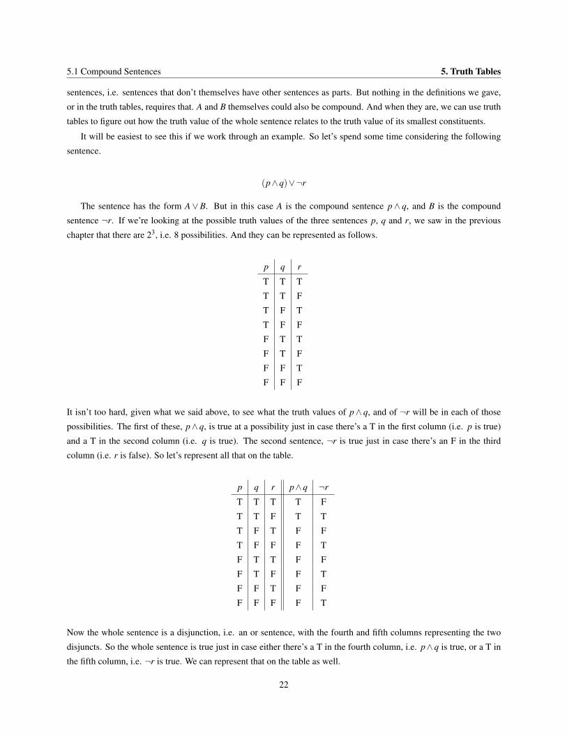
The sentence has the form A∨B. But in this case A is the compound sentence p∧ q, and B is the compound

sentence ¬r. If we’re looking at the possible truth values of the three sentences p, q and r, we saw in the previous

chapter that there are 23, i.e. 8 possibilities. And they can be represented as follows.

p q r

T T T

T T F

T F T

T F F

F T T

F T F

F F T

F F F

It isn’t too hard, given what we said above, to see what the truth values of p∧ q, and of ¬r will be in each of those

possibilities. The first of these, p∧q, is true at a possibility just in case there’s a T in the first column (i.e. p is true)

and a T in the second column (i.e. q is true). The second sentence, ¬r is true just in case there’s an F in the third

column (i.e. r is false). So let’s represent all that on the table.

p q r p∧q ¬r

T T T T F

T T F T T

T F T F F

T F F F T

F T T F F

F T F F T

F F T F F

F F F F T

Now the whole sentence is a disjunction, i.e. an or sentence, with the fourth and fifth columns representing the two

disjuncts. So the whole sentence is true just in case either there’s a T in the fourth column, i.e. p∧q is true, or a T in

the fifth column, i.e. ¬r is true. We can represent that on the table as well.

22

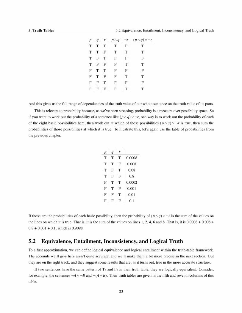
5. Truth Tables 5.2 Equivalence, Entailment, Inconsistency, and Logical Truth

p q r p∧q ¬r (p∧q)∨¬r

T T T T F T

T T F T T T

T F T F F F

T F F F T T

F T T F F F

F T F F T T

F F T F F F

F F F F T T

And this gives us the full range of dependencies of the truth value of our whole sentence on the truth value of its parts.

This is relevant to probability because, as we’ve been stressing, probability is a measure over possibility space. So

if you want to work out the probability of a sentence like (p∧q)∨¬r, one way is to work out the probability of each

of the eight basic possibilities here, then work out at which of those possibilities (p∧ q)∨¬r is true, then sum the

probabilities of those possibilities at which it is true. To illustrate this, let’s again use the table of probabilities from

the previous chapter.

p q r

T T T 0.0008

T T F 0.008

T F T 0.08

T F F 0.8

F T T 0.0002

F T F 0.001

F F T 0.01

F F F 0.1

If those are the probabilities of each basic possibility, then the probability of (p∧q)∨¬r is the sum of the values on

the lines on which it is true. That is, it is the sum of the values on lines 1, 2, 4, 6 and 8. That is, it is 0.0008 + 0.008 +

0.8 + 0.001 + 0.1, which is 0.9098.

5.2 Equivalence, Entailment, Inconsistency, and Logical TruthTo a first approximation, we can define logical equivalence and logical entailment within the truth-table framework.

The accounts we’ll give here aren’t quite accurate, and we’ll make them a bit more precise in the next section. But

they are on the right track, and they suggest some results that are, as it turns out, true in the more accurate structure.

If two sentences have the same pattern of Ts and Fs in their truth table, they are logically equivalent. Consider,

for example, the sentences ¬A∨¬B and ¬(A∧B). Their truth tables are given in the fifth and seventh columns of this

table.

23

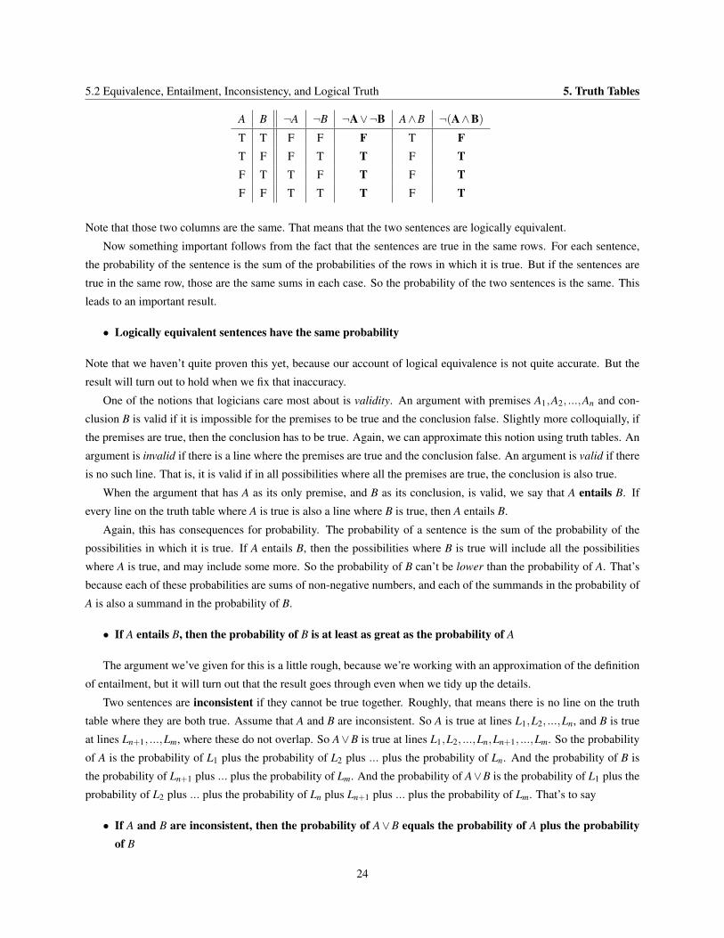
5.2 Equivalence, Entailment, Inconsistency, and Logical Truth 5. Truth Tables

A B ¬A ¬B ¬A∨¬B A∧B ¬(A∧B)

T T F F F T FT F F T T F TF T T F T F TF F T T T F T

Note that those two columns are the same. That means that the two sentences are logically equivalent.

Now something important follows from the fact that the sentences are true in the same rows. For each sentence,

the probability of the sentence is the sum of the probabilities of the rows in which it is true. But if the sentences are

true in the same row, those are the same sums in each case. So the probability of the two sentences is the same. This

leads to an important result.

• Logically equivalent sentences have the same probability

Note that we haven’t quite proven this yet, because our account of logical equivalence is not quite accurate. But the

result will turn out to hold when we fix that inaccuracy.

One of the notions that logicians care most about is validity. An argument with premises A1,A2, ...,An and con-

clusion B is valid if it is impossible for the premises to be true and the conclusion false. Slightly more colloquially, if

the premises are true, then the conclusion has to be true. Again, we can approximate this notion using truth tables. An

argument is invalid if there is a line where the premises are true and the conclusion false. An argument is valid if there

is no such line. That is, it is valid if in all possibilities where all the premises are true, the conclusion is also true.

When the argument that has A as its only premise, and B as its conclusion, is valid, we say that A entails B. If

every line on the truth table where A is true is also a line where B is true, then A entails B.

Again, this has consequences for probability. The probability of a sentence is the sum of the probability of the

possibilities in which it is true. If A entails B, then the possibilities where B is true will include all the possibilities

where A is true, and may include some more. So the probability of B can’t be lower than the probability of A. That’s

because each of these probabilities are sums of non-negative numbers, and each of the summands in the probability of

A is also a summand in the probability of B.

• If A entails B, then the probability of B is at least as great as the probability of A

The argument we’ve given for this is a little rough, because we’re working with an approximation of the definition

of entailment, but it will turn out that the result goes through even when we tidy up the details.

Two sentences are inconsistent if they cannot be true together. Roughly, that means there is no line on the truth

table where they are both true. Assume that A and B are inconsistent. So A is true at lines L1,L2, ...,Ln, and B is true

at lines Ln+1, ...,Lm, where these do not overlap. So A∨B is true at lines L1,L2, ...,Ln,Ln+1, ...,Lm. So the probability

of A is the probability of L1 plus the probability of L2 plus ... plus the probability of Ln. And the probability of B is

the probability of Ln+1 plus ... plus the probability of Lm. And the probability of A∨B is the probability of L1 plus the

probability of L2 plus ... plus the probability of Ln plus Ln+1 plus ... plus the probability of Lm. That’s to say

• If A and B are inconsistent, then the probability of A∨B equals the probability of A plus the probabilityof B

24

5. Truth Tables 5.3 Two Important Results

This is just the addition rule for measures transposed to probabilities. And it is a crucial rule, one that we will

use all the time. (Indeed, it is sometimes taken to be the characteristic axiom of probability theory. We will look at

axiomatic approaches to probability in the next chapter.)

Finally, a logical truth is something that is true in virtue of logic alone. It is true in all possibilities, since what

logic is does not change. A logical truth is entailed by any sentence. And a logical truth only entails other sentences.

Any sentence that is true in all possibilities must have probability 1. That’s because probability is a normalised

measure, and in a normalised measure, the measure of the universe is 1. And a logical truth is true at every point in

the ‘universe’ of logical space.

• Any logical truth has probability 1

5.3 Two Important ResultsNone of the three connectives is particularly hard to process, but the rule for negation may well be the easiest of the

lot. The truth value of ¬A is just the opposite of the truth value of A. So if A is true at a line, then ¬A is false. And if

A is false at a line, then ¬A is true. So exactly one of A and ¬A is true at each line. So the sum of the probabilities of

those propositions must be 1.

We can get to this result another way. It is easy to see that A∨¬A is a logical truth by simply looking at its truth

table.

A ¬A A∨¬A

T F T

F T T

The sentence A∨¬A is true on each line, so it is a logical truth. And logical truths have probability 1. Now A and

¬A are clearly inconsistent. So the probability of their disjunction equals the sum of their probabilities. That’s to say,

Pr(A∨¬A) = Pr(A)+Pr(¬A). But Pr(A∨¬A) = 1. So,

Pr(A)+Pr(¬A) = 1

One important consequence of this is that the probabilities of A and ¬A can’t vary independently. Knowing how

probable A is settles how probable ¬A is.

The next result is slightly more complicated, but only a little. Consider the following table of truth values and

probabilities.

Pr A B A∧B A∨B

x1 T T T T

x2 T F F T

x3 F T F T

x4 F F F F

The variables in the first column represent the probability of each row. We can see from the table that the following

results all hold.

25

5.3 Two Important Results 5. Truth Tables

1. Pr(A) = x1 + x2, since A is true on the first and second lines

2. Pr(B) = x1 + x3, since B is true on the first and third lines

3. Pr(A∧B) = x1, since A∧B is true on the first line

4. Pr(A∨B) = x1 + x2 + x3, since A∨B is true on the first, second and third lines

Adding the first and second lines together, we get

Pr(A)+Pr(B) = x1 + x2 + x1 + x3

And adding the third and fourth lines together, we get

Pr(A∧B)+Pr(A∨B) = x1 + x1 + x2 + x3

And simply rearranging the variables a little reveals that

Pr(A)+Pr(B) = Pr(A∧B)+Pr(A∨B)

Again, this is a result that we will use a lot in what follows.

26

Chapter 6 Axioms for Probability

6.1 Axioms of ProbabilityWe’ve introduced probability so far through the truth tables. If you are concerned with some finite number, say n

of sentences, you can make up a truth table with 2n rows representing all the possible combinations of truth values

for those sentences. And then a probability function is simply a measure defined over sets of those rows, i.e. sets of

possibilities.

But we can also introduce probability more directly. A probability function is a function that takes sentences as

inputs, has outputs in [0, 1], and satisfies the following constraints.

• If A is a logical truth, then Pr(A) = 1

• If A and B are logically equivalent, then Pr(A) = Pr(B)

• If A and B are logically disjoint, i.e. ¬(A∧B) is a logical truth, then Pr(A)+Pr(B) = Pr(A∨B)

To get a feel for how these axioms operate, I’ll run through a few proofs using the axioms. The results we prove

will be familiar from the previous chapter, but the interest here is in seeing how the axioms interact with the definitions

of logical truth, logical equivalence and logical disjointedness to derive familiar results.

• Pr(A)+Pr(¬A) = 1

Proof: It is a logical truth that A∨¬A. This can be easily seen on a truth table. So by axiom 1, Pr(A∨¬A) = 1. The

truth tables can also be used to show that ¬(A∧A) is a logical truth, so A and ¬A are disjoint. So Pr(A)+Pr(¬A) =

Pr(A∨¬A). But since Pr(A∨¬A) = 1, it follows that Pr(A)+Pr(¬A) = 1.

• If A is a logical falsehood, i.e. ¬A is a logical truth, then Pr(A) = 0

Proof: If ¬A is a logical truth, then by axiom 1, Pr(¬A) = 1. We just proved that Pr(A)+ Pr(¬A) = 1. From this it

follows that Pr(A) = 0.

• Pr(A)+Pr(B) = Pr(A∨B)+Pr(A∧B)

Proof: First, note that A is logically equivalent to (A∧B)∨ (A∧¬B), and that (A∧B) and (A∧¬B) are logically

disjoint. We can see both these facts in the following truth table.

A B ¬B (A∧B) (A∧¬B) (A∧B)∨ (A∧¬B)

T T F T F T

T F T F T T

F T F F F F

F F T F F F

27

6.2 Truth Tables and Possibilities 6. Axioms for Probability

The first and sixth columns are identical, so A and (A∧B)∨ (A∧¬B). By axiom 2, that means that Pr(A) = Pr((A∧B)∨ (A∧¬B)).

The fourth and fifth column never have a T on the same row, so (A∧B) and (A∧¬B) are disjoint. That means that

Pr((A∧B)∨ (A∧¬B) = Pr((A∧B)+Pr(A∧¬B). Putting the two results together, we get that Pr(A) = Pr((A∧B)+

Pr(A∧¬B).

The next truth table is designed to get us two results. First, that A∨B is equivalent to B∨ (A∧¬B). And second

that B and (A∧¬B) are disjoint.

A B A∨B ¬B A∧¬B B∨ (A∧¬B)

T T T F F T

T F T T T T

F T T F F T

F F F T F F

Note that the third column, A∨B, and the sixth column, B∨ (A∧¬B), are identical. So those two propositions are

equivalent. So Pr(A∨B) = Pr(B∨ (A∧¬B)).

Note also that the second column, B and the fifth column, A∧¬B, have no Ts in common. So they are disjoint. So

Pr(B∨ (A∧¬B)) = Pr(B)+Pr(A∧¬B). Putting the last two results together, we get that Pr(A∨B) = Pr(B)+Pr(A∧¬B).

If we add Pr(A∧B) to both sides of that last equation, we get Pr(A∨B)+Pr(A∧B) = Pr(B)+Pr(A∧¬B)+Pr(A∧B). But note that we already proved that Pr(A∧¬B)+Pr(A∧B) = Pr(A). So we can rewrite Pr(A∨B)+Pr(A∧B) =

Pr(B)+ Pr(A∧¬B)+ Pr(A∧B) as Pr(A∨B)+ Pr(A∧B) = Pr(B)+ Pr(A). And simply rearranging terms around

gives us Pr(A)+Pr(B) = Pr(A∨B)+Pr(A∧B), which is what we set out to prove.

6.2 Truth Tables and PossibilitiesSo far we’ve been assuming that whenever we are interested in n sentences, there are 2n possibilities. But this isn’t

always the case. Sometimes a combination of truth values doesn’t express a real possibility. Consider, for example,

the case where A = Many people enjoyed the play, and B = Some people enjoyed the play. Now we might start trying

to draw up a truth table as follows.

A B

T T

T F

F T

F F

But there’s something deeply wrong with this table. The second line doesn’t represent a real possibility. It isn’t

possible that it’s true that many people enjoyed the play, but false that some people enjoyed the play. In fact there are

only three real possibilities here. First, many people (and hence some people) enjoyed the play. Second, some people,

but not many people, enjoyed the play. Third, no one enjoyed the play. That’s all the possibilities that there are. There

isn’t a fourth possibility.

28

6. Axioms for Probability 6.2 Truth Tables and Possibilities

In this case, A entails B, which is why there is no possibility where A is true and B is false. In other cases there

might be more complicated interrelations between sentences that account for some of the lines not representing real

possibilities. Consider, for instance, the following case.

• A = Alice is taller than Betty

• B = Betty is taller than Carla

• C = Carla is taller than Alice

Again, we might try and have a regular, 8 line, truth table for these, as below.

A B C

T T T

T T F

T F T

T F F

F T T

F T F

F F T

F F F

But here the first line is not a genuine possibility. If Alice is taller than Betty, and Betty is taller than Carla, then Carla

can’t be taller than Alice. So there are, at most, 7 real possibilities here. (We’ll leave the question of whether there are

fewer than 7 possibilities as an exercise.) Again, one of the apparent possibilities is not real.

The chance that there are lines on the truth tables that don’t represent real possibilities means that we have to

modify several of the definitions we offered above. More carefully, we should say.

• Two sentences are A and B are logically equivalent if (and only if) they have the same truth value at every line

on the truth table that represents a real possibility.

• Some sentences A1, ...,An entail a sentence B if (and only if) at every line which (a) represents a real possibility

and (b) each of A1, ...,An is true, B is true. Another way of putting this is that the argument from A1, ...,An to B

is valid.

• Two sentences A and B are logically disjoint if (and only if) there is no line which (a) represents a real possibility

and (b) they are both true at that line

Surprisingly perhaps, we don’t have to change the definition of a probability function all that much. We started off

by saying that you got a probability function, defined over A1,An by starting with the truth table for those sentences,

all 2n rows of it, and assigning numbers to each row in a way that they added up to 1. The probability of any sentence

was then the sum of the numbers assigned to each row at which it is true.

This needs to be changed a little. If something does not represent a real possibility, then its negation is a logical

truth. And all logical truths have to get probability 1. So we have to assign 0 to every row that does not represent a

real possibility.

29

6.3 Propositions and Possibilities 6. Axioms for Probability

But that’s the only change we have to make. Still, any way of assigning numbers to rows such that the numbers

sum to 1, and any row that does not represent a real possibility is assigned 0, will be a probability function. And, as

long as we are only interested in sentences with A1,An as parts, any probability function can be generated this way.

So in fact all of the proofs in the previous handout will still go through. There we generated a lot of results from

the assumption that any probability function is a measure over the possibility space generated by a truth table. And

that assumption is, strictly speaking, true. Any probability function is a measure over the possibility space generated

by a truth table. It’s true that some such measures are not probability functions because they assign positive values to

lines that don’t represent real possibilities. But that doesn’t matter for the proofs we were making there.

The upshot is that we can, for the purposes of decision theory, continue to think about probability functions using

truth tables. Occasionally we will have to be a little more careful, but for the most part, just assigning numbers to rows

gives us all the basic probability theory we will need.

6.3 Propositions and PossibilitiesThere are many things we can be uncertain about. Some of these concern matters of fact, especially facts about the

future. We can be uncertain about horseraces, or elections, or the weather. And some of them concern matters to do

with mathematics or logic. We might be uncertain about whether two propositions are logically equivalent. Or we

might be uncertain whether a particular mathematical conjecture is true or false.

Sometimes our uncertainty about a subject matter relates to both things. I’m writing this in the middle of hurricane

season, and we’re frequently uncertain about what the hurricanes will do. There are computer models to predict them,

but the models are very complicated, and take hours to produce results even once all the data is in. So we might also

be uncertain about a purely mathematical fact, namely what this model will predict given these inputs.

One of the consequences of the axioms for probability theory we gave above is that any logical truth, and for current

purposes at least mathematical truths count as logical truths, get probability 1. This might seem counterintuitive.

Surely we can sensibly say that such and such a mathematical claim is likely to be true, or probable to be true. Or

we can say that someone’s logical conjecture is probably false. How could it be that the axioms of probability say

otherwise?

Well, the important thing to remember here is that what we’re developing is a formal, mathematical notion. It

remains an open question, indeed a deep philosophical question, whether that mathematical notion is useful in making

sense of our intuitive, informal notion of what’s more or less likely, or more or less probable. It is natural to think

at this point that probability theory, the mathematical version, will not be of much help in modelling our uncertainty

about logic or mathematics.

At one level this should not be too surprising. In order to use a logical/mathematical model, we have to use logic

and mathematics. And to use logic and mathematics, we have to presuppose that they are given and available to use.

But that’s very close already to presupposing that they aren’t at all uncertain. Now this little argument isn’t very

formal, and it certainly isn’t meant to be a conclusive proof that there couldn’t be a mathematical model of uncertainty

about mathematics. But it’s a reason to think that such a model would have to solve some tricky conceptual questions

that a model of uncertainty about the facts does not have to solve.

And not only should this not be surprising, it should not necessarily be too worrying. In decision theory, what we’re

usually concerned with is uncertainty about the facts. It’s possible that probability theory can be the foundation for

an excellent model for uncertainty about the facts even if such a model is a terrible tool for understanding uncertainty

30

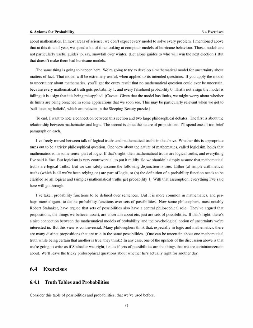
6. Axioms for Probability 6.4 Exercises

about mathematics. In most areas of science, we don’t expect every model to solve every problem. I mentioned above

that at this time of year, we spend a lot of time looking at computer models of hurricane behaviour. Those models are

not particularly useful guides to, say, snowfall over winter. (Let alone guides to who will win the next election.) But

that doesn’t make them bad hurricane models.

The same thing is going to happen here. We’re going to try to develop a mathematical model for uncertainty about

matters of fact. That model will be extremely useful, when applied to its intended questions. If you apply the model

to uncertainty about mathematics, you’ll get the crazy result that no mathematical question could ever be uncertain,

because every mathematical truth gets probability 1, and every falsehood probability 0. That’s not a sign the model is

failing; it is a sign that it is being misapplied. (Caveat: Given that the model has limits, we might worry about whether

its limits are being breached in some applications that we soon see. This may be particularly relevant when we get to

‘self-locating beliefs’, which are relevant in the Sleeping Beauty puzzle.)

To end, I want to note a connection between this section and two large philosophical debates. The first is about the

relationship between mathematics and logic. The second is about the nature of propositions. I’ll spend one all-too-brief

paragraph on each.

I’ve freely moved between talk of logical truths and mathematical truths in the above. Whether this is appropriate

turns out to be a tricky philosophical question. One view about the nature of mathematics, called logicisim, holds that

mathematics is, in some sense, part of logic. If that’s right, then mathematical truths are logical truths, and everything

I’ve said is fine. But logicism is very controversial, to put it mildly. So we shouldn’t simply assume that mathematical

truths are logical truths. But we can safely assume the following disjunction is true. Either (a) simple arithmetical

truths (which is all we’ve been relying on) are part of logic, or (b) the definition of a probability function needs to be

clarified so all logical and (simple) mathematical truths get probability 1. With that assumption, everything I’ve said

here will go through.

I’ve taken probability functions to be defined over sentences. But it is more common in mathematics, and per-

haps more elegant, to define probability functions over sets of possibilities. Now some philosophers, most notably

Robert Stalnaker, have argued that sets of possibilities also have a central philosophical role. They’ve argued that

propositions, the things we believe, assert, are uncertain about etc, just are sets of possibilities. If that’s right, there’s

a nice connection between the mathematical models of probability, and the psychological notion of uncertainty we’re

interested in. But this view is controversial. Many philosophers think that, especially in logic and mathematics, there

are many distinct propositions that are true in the same possibilities. (One can be uncertain about one mathematical

truth while being certain that another is true, they think.) In any case, one of the upshots of the discussion above is that

we’re going to write as if Stalnaker was right, i.e. as if sets of possibilities are the things that we are certain/uncertain

about. We’ll leave the tricky philosophical questions about whether he’s actually right for another day.

6.4 Exercises

6.4.1 Truth Tables and Probabilities

Consider this table of possibilities and probabilities, that we’ve used before.

31

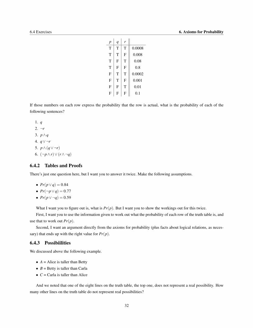
6.4 Exercises 6. Axioms for Probability

p q r

T T T 0.0008

T T F 0.008

T F T 0.08

T F F 0.8

F T T 0.0002

F T F 0.001

F F T 0.01

F F F 0.1

If those numbers on each row express the probability that the row is actual, what is the probability of each of the

following sentences?

1. q

2. ¬r

3. p∧q

4. q∨¬r

5. p∧ (q∨¬r)

6. (¬p∧ r)∨ (r∧¬q)

6.4.2 Tables and Proofs

There’s just one question here, but I want you to answer it twice. Make the following assumptions.

• Pr(p∨q) = 0.84

• Pr(¬p∨q) = 0.77

• Pr(p∨¬q) = 0.59

What I want you to figure out is, what is Pr(p). But I want you to show the workings out for this twice.

First, I want you to use the information given to work out what the probability of each row of the truth table is, and

use that to work out Pr(p).

Second, I want an argument directly from the axioms for probability (plus facts about logical relations, as neces-

sary) that ends up with the right value for Pr(p).

6.4.3 Possibiilities

We discussed above the following example.

• A = Alice is taller than Betty

• B = Betty is taller than Carla

• C = Carla is taller than Alice

And we noted that one of the eight lines on the truth table, the top one, does not represent a real possibility. How

many other lines on the truth table do not represent real possibilities?

32

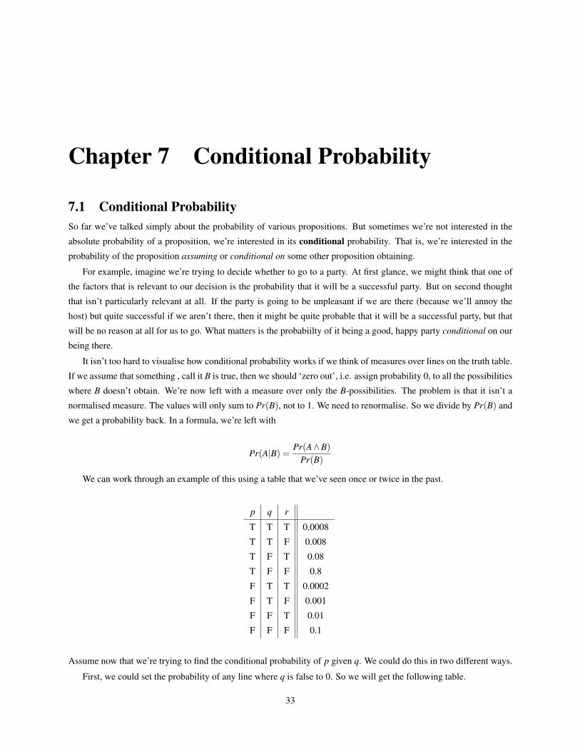
Chapter 7 Conditional Probability

7.1 Conditional ProbabilitySo far we’ve talked simply about the probability of various propositions. But sometimes we’re not interested in the

absolute probability of a proposition, we’re interested in its conditional probability. That is, we’re interested in the

probability of the proposition assuming or conditional on some other proposition obtaining.

For example, imagine we’re trying to decide whether to go to a party. At first glance, we might think that one of

the factors that is relevant to our decision is the probability that it will be a successful party. But on second thought

that isn’t particularly relevant at all. If the party is going to be unpleasant if we are there (because we’ll annoy the

host) but quite successful if we aren’t there, then it might be quite probable that it will be a successful party, but that

will be no reason at all for us to go. What matters is the probabiilty of it being a good, happy party conditional on our

being there.

It isn’t too hard to visualise how conditional probability works if we think of measures over lines on the truth table.

If we assume that something , call it B is true, then we should ‘zero out’, i.e. assign probability 0, to all the possibilities

where B doesn’t obtain. We’re now left with a measure over only the B-possibilities. The problem is that it isn’t a

normalised measure. The values will only sum to Pr(B), not to 1. We need to renormalise. So we divide by Pr(B) and

we get a probability back. In a formula, we’re left with

Pr(A|B) =Pr(A∧B)

Pr(B)

We can work through an example of this using a table that we’ve seen once or twice in the past.

p q r

T T T 0.0008

T T F 0.008

T F T 0.08

T F F 0.8

F T T 0.0002

F T F 0.001

F F T 0.01

F F F 0.1

Assume now that we’re trying to find the conditional probability of p given q. We could do this in two different ways.

First, we could set the probability of any line where q is false to 0. So we will get the following table.

33

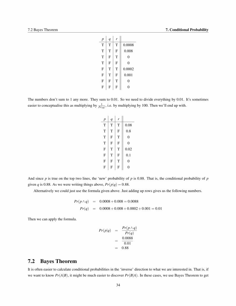
7.2 Bayes Theorem 7. Conditional Probability

p q r

T T T 0.0008

T T F 0.008

T F T 0

T F F 0

F T T 0.0002

F T F 0.001

F F T 0

F F F 0

The numbers don’t sum to 1 any more. They sum to 0.01. So we need to divide everything by 0.01. It’s sometimes

easier to conceptualise this as multiplying by 1Pr(q) , i.e. by multiplying by 100. Then we’ll end up with.

p q r

T T T 0.08

T T F 0.8

T F T 0

T F F 0

F T T 0.02

F T F 0.1

F F T 0

F F F 0

And since p is true on the top two lines, the ‘new’ probability of p is 0.88. That is, the conditional probability of p

given q is 0.88. As we were writing things above, Pr(p|q) = 0.88.

Alternatively we could just use the formula given above. Just adding up rows gives us the following numbers.

Pr(p∧q) = 0.0008+0.008 = 0.0088

Pr(q) = 0.0008+0.008+0.0002+0.001 = 0.01

Then we can apply the formula.

Pr(p|q) =Pr(p∧q)

Pr(q)

=0.0088

0.01= 0.88

7.2 Bayes TheoremIt is often easier to calculate conditional probabilities in the ‘inverse’ direction to what we are interested in. That is, if

we want to know Pr(A|B), it might be much easier to discover Pr(B|A). In these cases, we use Bayes Theorem to get

34

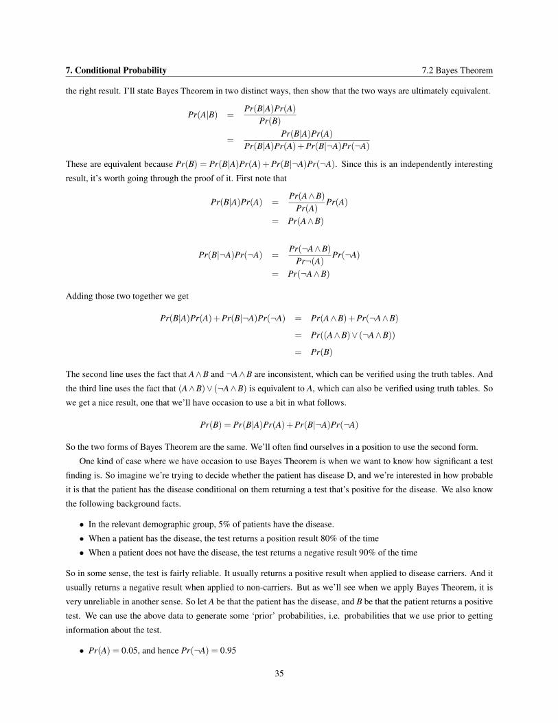
7. Conditional Probability 7.2 Bayes Theorem

the right result. I’ll state Bayes Theorem in two distinct ways, then show that the two ways are ultimately equivalent.

Pr(A|B) =Pr(B|A)Pr(A)

Pr(B)

=Pr(B|A)Pr(A)

Pr(B|A)Pr(A)+Pr(B|¬A)Pr(¬A)

These are equivalent because Pr(B) = Pr(B|A)Pr(A)+ Pr(B|¬A)Pr(¬A). Since this is an independently interesting

result, it’s worth going through the proof of it. First note that

Pr(B|A)Pr(A) =Pr(A∧B)

Pr(A)Pr(A)

= Pr(A∧B)

Pr(B|¬A)Pr(¬A) =Pr(¬A∧B)

Pr¬(A)Pr(¬A)

= Pr(¬A∧B)

Adding those two together we get

Pr(B|A)Pr(A)+Pr(B|¬A)Pr(¬A) = Pr(A∧B)+Pr(¬A∧B)

= Pr((A∧B)∨ (¬A∧B))

= Pr(B)

The second line uses the fact that A∧B and ¬A∧B are inconsistent, which can be verified using the truth tables. And

the third line uses the fact that (A∧B)∨ (¬A∧B) is equivalent to A, which can also be verified using truth tables. So

we get a nice result, one that we’ll have occasion to use a bit in what follows.

Pr(B) = Pr(B|A)Pr(A)+Pr(B|¬A)Pr(¬A)

So the two forms of Bayes Theorem are the same. We’ll often find ourselves in a position to use the second form.

One kind of case where we have occasion to use Bayes Theorem is when we want to know how significant a test

finding is. So imagine we’re trying to decide whether the patient has disease D, and we’re interested in how probable

it is that the patient has the disease conditional on them returning a test that’s positive for the disease. We also know

the following background facts.

• In the relevant demographic group, 5% of patients have the disease.

• When a patient has the disease, the test returns a position result 80% of the time

• When a patient does not have the disease, the test returns a negative result 90% of the time

So in some sense, the test is fairly reliable. It usually returns a positive result when applied to disease carriers. And it

usually returns a negative result when applied to non-carriers. But as we’ll see when we apply Bayes Theorem, it is

very unreliable in another sense. So let A be that the patient has the disease, and B be that the patient returns a positive

test. We can use the above data to generate some ‘prior’ probabilities, i.e. probabilities that we use prior to getting

information about the test.

• Pr(A) = 0.05, and hence Pr(¬A) = 0.95

35

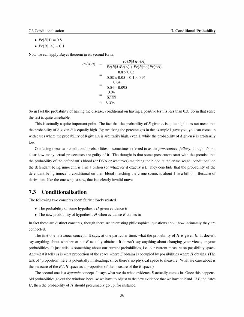
7.3 Conditionalisation 7. Conditional Probability

• Pr(B|A) = 0.8

• Pr(B|¬A) = 0.1

Now we can apply Bayes theorem in its second form.

Pr(A|B) =Pr(B|A)Pr(A)

Pr(B|A)Pr(A)+Pr(B|¬A)Pr(¬A)

=0.8×0.05

0.08×0.05+0.1×0.95

=0.04

0.04+0.095

=0.04

0.135≈ 0.296

So in fact the probability of having the disease, conditional on having a positive test, is less than 0.3. So in that sense

the test is quite unreliable.

This is actually a quite important point. The fact that the probability of B given A is quite high does not mean that

the probability of A given B is equally high. By tweaking the percentages in the example I gave you, you can come up

with cases where the probability of B given A is arbitrarily high, even 1, while the probability of A given B is arbitrarily

low.

Confusing these two conditional probabilities is sometimes referred to as the prosecutors’ fallacy, though it’s not

clear how many actual prosecutors are guilty of it! The thought is that some prosecutors start with the premise that

the probability of the defendant’s blood (or DNA or whatever) matching the blood at the crime scene, conditional on

the defendant being innocent, is 1 in a billion (or whatever it exactly is). They conclude that the probability of the

defendant being innocent, conditional on their blood matching the crime scene, is about 1 in a billion. Because of

derivations like the one we just saw, that is a clearly invalid move.

7.3 ConditionalisationThe following two concepts seem fairly closely related.

• The probability of some hypothesis H given evidence E

• The new probability of hypothesis H when evidence E comes in

In fact these are distinct concepts, though there are interesting philosophical questions about how intimately they are

connected.

The first one is a static concept. It says, at one particular time, what the probability of H is given E. It doesn’t

say anything about whether or not E actually obtains. It doesn’t say anything about changing your views, or your

probabilities. It just tells us something about our current probabilities, i.e. our current measure on possibility space.

And what it tells us is what proportion of the space where E obtains is occupied by possibilities where H obtains. (The

talk of ‘proportion’ here is potentially misleading, since there’s no physical space to measure. What we care about is

the measure of the E ∧H space as a proportion of the measure of the E space.)

The second one is a dynamic concept. It says what we do when evidence E actually comes in. Once this happens,

old probabilities go out the window, because we have to adjust to the new evidence that we have to hand. If E indicates

H, then the probability of H should presumably go up, for instance.

36

7. Conditional Probability 7.3 Conditionalisation

Because these are two distinct concepts, we’ll have two different symbols for them. We’ll use Pr(H|E) for the

static concept, and PrE(H) for the dynamic concept. So Pr(H|E) is what the current probability of H given E is, and

PrE(H) is what the probability of H will be when we get evidence E.

Many philosophers think that these two should go together. More precisely, they think that a rational agent always

updates by conditionalisation. That’s just to say that for any rational agent, Pr(H|E) = PrE(H). When we get evidence

E, we always replace the probability of H with the probability of H given E.

The conditionalisation thesis occupies a quirky place in contemporary philosophy. On the one hand it is almost

universally accepted, and an extremely interesting set of theoretical results have been built up using the assumption it

is true. (Pretty much everything in Bayesian philosophy of science relies in one way or another on the assumption that

conditionalisation is correct. And since Bayesian philosophy of science is a thriving research program, this is a non-

trivial fact.) On the other hand, there are remarkably few direct, and plausible, arguments in favor of conditionalisation.

In the absence of a direct argument we can say two things.

First, the fact that a lot of philosophers (and statisticians and economists etc) accept conditionalisation, and have

derived many important results using it, is a reason to take it seriously. The research programs that are based around

conditionalisation do not seem to be degenerating, or failing to produce new insights. Second, in a lot of everyday

applications, conditionalisation seems to yield sensible results. The simplest cases here are cases involving card games

or roulette wheels where we can specify the probabilities of various outcomes in advance.

Let’s work through a very simple example to see this. A deck of cards has 52 cards, of which 13 are hearts. Imagine

we’re about to draw 2 cards, without replacement, from that deck, which has been well-shuffled. The probability that

the first is a heart is 1352 , or, more simply, 1

4 . If we assume that a heart has been taken out, e.g. if we draw a heart with

the first card, the probability that we’ll draw another heart if 1251 . That is, conditional on the first card we draw being a

heart, the probability that the second is a heart if 1251 .

Now imagine that we do actually draw the first card, and it’s a heart. What should the probability be that the next

card will be a heart? It seems like it should be 1251 . Indeed, it is hard to see what else it could be. If A is The first card

drawn is a heart and B is The second card drawn is a heart, then it seems both Pr(A|B) and PrB(A) should be 1251 . And

examples like this could be multiplied endlessly.

The support here for conditionalisation is not just that we ended up with the same result. It’s that we seem to

be making the same calculations both times. In cases like this, when we’re trying to figure out Pr(A|B), we pretend

we’re trying to work out PrB(A), and then stop pretending when we’ve worked out the calculation. If that’s always the

right way to work out Pr(A|B), then Pr(A|B) should always turn out to be equal to PrB(A). Now this argument goes

by fairly quickly obviously, and we might want to look over more details later on, but it’s easy to see we might take

conditionalisation to be a plausible model for updating probabilities.

37

7.3 Conditionalisation 7. Conditional Probability

38

Chapter 8 About Conditional Probability

8.1 ConglomerabilityHere is a feature that we’d like an updating rule to have. If getting some evidence E will make a hypothesis H more

probable, then not getting E will not also make H more probable. Indeed, in standard cases, not getting evidence that

would have made H more probable should make H less probable. It would be very surprising if we could know, before

running a test, that however it turns out some hypothesis H will be more probable at the end of the test than at the

beginning of it. We might have to qualify this in odd cases where H is, e.g., that the test is completed. But in standard

cases if H will be likely whether some evidence comes in or doesn’t come in, then H should be already likely.

We’ll say that an update rule is conglomerable if it has this feature, and non-conglomerable otherwise. That is,

it is non-conglomerable iff there are H and E such that,

PrE(H) > Pr(H)andPr¬E(H) > Pr(H)

Now a happy result for conditionalisation, the rule that says PE(H) = Pr(H|E), is that it is conglomerable. This result

is worth going over in some detail. Assume that Pr(H|E) > Pr(H)andPr¬E(H) > Pr(H). Then we can derive a

contradicton as follows

Pr(H) = Pr((H ∧E)∨ (H ∧¬E)) since H = (H ∧E)∨ (H ∧¬E)

= Pr(H ∧E)+Pr(H ∧¬E) since (H ∧E) and (H ∧¬E) are disjoint

= Pr(H|E)Pr(E)+Pr(H|¬E)Pr(¬E) since Pr(H|E)Pr(E) = Pr(H ∧E)

> Pr(H)Pr(E)+Pr(H)Pr(¬E) since by assumption Pr(H|E) > Pr(H) and Pr(H|¬E) > Pr(H)

= Pr(H)(Pr(E)+Pr(¬E))

= Pr(H)Pr(E ∨¬E) since E and ¬E are disjoint

= Pr(H) since Pr(E ∨¬E) = 1

Conglomerability is related to dominance. The dominance rule of decision making says (among other things) that if C1

is preferable to C2 given E, and C1 is preferable to C2 given ¬E, then C1 is simply preferable to C2. Conglomerability

says (among other things) that if Pr(H) is greater than x given E, and it is greater than x given ¬E, then it is simply

greater than x.

Contemporary decision theory makes deep and essential use of principles of this form, i.e. that if something

holds given E, and given ¬E, then it simply holds. And one of the running themes of these notes will be sorting out

just which such principles hold, and which do not hold. The above proof shows that we get one nice result relating

conditional probability and simple probability which we can rely on.

39

8.2 Independence 8. About Conditional Probability

8.2 IndependenceThe probability of some propositions depends on other propositions. The probability that I’ll be happy on Monday

morning is not independent of whether I win the lottery on the weekend. On the other hand, the probability that

I win the lottery on the weekend is independent of whether it rains in Seattle next weekend. Formally, we define

probabilistic indepdendence as follows.

• Propositions A and B are independent iff Pr(A|B) = Pr(A).

There is something odd about this definition. We purported to define a relationship that holds between pairs of

propositions. It looked like it should be a symmetric relation: A is independent from B iff B is independent from A.

But the definition looks asymmetric: A and B play very different roles on the right-hand side of the definition. Happily,

this is just an appearance. Assuming that A and B both have positive probability, we can show that Pr(A|B) = Pr(A)

is equivalent to Pr(B|A) = Pr(B).

Pr(A|B) = Pr(A)

⇔ Pr(A∧B)Pr(B)

= Pr(A)

⇔ Pr(A∧B) = Pr(A)×Pr(B)

⇔ Pr(A∧B)Pr(A)

= Pr(B)

⇔ Pr(B|A) = Pr(B)

We’ve multiplied and divided by Pr(A) and Pr(B), so these equivalences don’t hold if Pr(A) or Pr(B) is 0. But in

other cases, it turns out that Pr(A|B) = Pr(A) is equivalent to Pr(B|A) = Pr(B). And each of these is equivalent to the

claim that Pr(A∧B) = Pr(A)Pr(B). This is an important result, and one that we’ll refer to a bit.

• For independent propositions, the probability of their conjunction is the product of their probabilities.

• That is, if A and B are independent, then Pr(A∧B) = Pr(A)Pr(B)

This rule doesn’t apply in cases where A and B are dependent. To take an extreme case, when A is equivalent to

B, then A∧B is equivalent to A. In that case, Pr(A∧B) = Pr(A), not Pr(A)2. So we have to be careful applying this

multiplication rule. But it is a powerful rule in those cases where it works.

8.3 Kinds of IndependenceThe formula Pr(A|B) = Pr(A) is, by definition, what probabilistic independence amounts to. It’s important to note

that probabilistic dependence is very different from causal dependence, and so we’ll spend a bit of time going over the

differences.

The phrase ‘causal dependence’ is a little ambiguous, but one natural way to use it is that A causally depends on B

just in case B causes A. If we use it that way, it is an asymmetric relation. If B causes A, then A doesn’t cause B. But

probabilistic dependence is symmetric. That’s what we proved in the previous section.

40

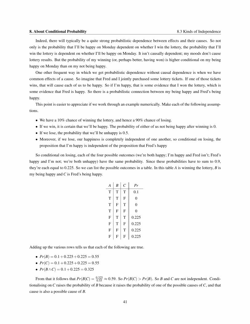
8. About Conditional Probability 8.3 Kinds of Independence

Indeed, there will typically be a quite strong probabilistic dependence between effects and their causes. So not

only is the probability that I’ll be happy on Monday dependent on whether I win the lottery, the probability that I’ll

win the lottery is dependent on whether I’ll be happy on Monday. It isn’t causally dependent; my moods don’t cause

lottery results. But the probability of my winning (or, perhaps better, having won) is higher conditional on my being

happy on Monday than on my not being happy.

One other frequent way in which we get probabilistic dependence without causal dependence is when we have

common effects of a cause. So imagine that Fred and I jointly purchased some lottery tickets. If one of those tickets

wins, that will cause each of us to be happy. So if I’m happy, that is some evidence that I won the lottery, which is

some evidence that Fred is happy. So there is a probabilistic connection between my being happy and Fred’s being

happy.

This point is easier to appreciate if we work through an example numerically. Make each of the following assump-

tions.

• We have a 10% chance of winning the lottery, and hence a 90% chance of losing.

• If we win, it is certain that we’ll be happy. The probability of either of us not being happy after winning is 0.

• If we lose, the probability that we’ll be unhappy is 0.5.

• Moreover, if we lose, our happiness is completely independent of one another, so conditional on losing, the

proposition that I’m happy is independent of the proposition that Fred’s happy

So conditional on losing, each of the four possible outcomes (we’re both happy; I’m happy and Fred isn’t; Fred’s

happy and I’m not; we’re both unhappy) have the same probability. Since these probabilities have to sum to 0.9,

they’re each equal to 0.225. So we can list the possible outcomes in a table. In this table A is winning the lottery, B is

my being happy and C is Fred’s being happy.

A B C Pr

T T T 0.1

T T F 0

T F T 0

T F F 0

F T T 0.225

F T F 0.225

F F T 0.225

F F F 0.225

Adding up the various rows tells us that each of the following are true.

• Pr(B) = 0.1+0.225+0.225 = 0.55

• Pr(C) = 0.1+0.225+0.225 = 0.55

• Pr(B∧C) = 0.1+0.225 = 0.325

From that it follows that Pr(B|C) = 0.3250.55 ≈ 0.59. So Pr(B|C) > Pr(B). So B and C are not independent. Condi-

tionalising on C raises the probability of B because it raises the probability of one of the possible causes of C, and that

cause is also a possible cause of B.

41

8.4 Gamblers’ Fallacy 8. About Conditional Probability

Often we know a lot more about probabilistic dependence than we know about causal connections and we have

work to do to figure out the causal connections. It’s very hard, especially in for example public health settings, to

figure out what is a cause-effect pair, and what is the result of a common cause. One of the most important research

programs in modern statistics is developing methods for solving just this problem. The details of those methods won’t

concern us here, but we’ll just note that there’s a big gap between probabilistic dependence and causal dependence.

On the other hand, it is usually safe to infer probabilistic dependence from causal dependence. If E is one of the

(possible) causes of H, then usually E will change the probabilities of H. We can perhaps dimly imagine exceptions

to this rule.

So imagine that a quarterback is trying to decide whether to run or pass on the final play of a football game. He

decides to pass, and the pass is successful, and his team wins. Now as it happens, had he decided to run, the team

would have had just as good a chance of winning, since their run game was exactly as likely to score as their pass

game. It’s not crazy to think in those circumstances that the decision to pass was among the causes of the win, but

the win was probabilistically independent of the decision to pass. In general we can imagine cases where some event

moves a process down one of two possible paths to success, and where the other path had just as good a chance of

success. (Imagine a doctor deciding to operate in a certain way, a politician campaigning in one area rather than

another, a storm moving a battle from one piece of land to another, or any number of such cases.) In these cases we

might have causal dependence (though whether we do is a contentious issue in the metaphysics of causation) without

probabilistic dependence.

But such cases are rare at best. It is a completely commonplace occurrence to have probabilistic dependence

without clear lines of causal dependence. We have to have very delicately balanced states of the world in order to

have causal dependence without probabilistic dependence, and in every day cases we can safely assume that such a

situation is impossible.ut of probabilistic connections

8.4 Gamblers’ FallacyIf some events are independent, then the probability of one is independent of the probability of the others. So knowing

the results of one event gives you no guidance, not even probabilistic guidance, into whether the other will happen.

These points may seem completely banal, but in fact they are very hard to fully incorporate into our dails lives.

In particular, they are very hard to completely incorporate in cases where we are dealing with successive outcomes of

a particular chance process, such as a dice roll or a coin flip. In those cases we know that the individual events are

independent of one another. But it’s very hard not to think that, after a long run of heads say, that the coin landing tails

is ‘due’.

This feeling is what is known as the Gamblers’ Fallacy. It is the fallacy of thinking that, when events A and B are

independent, that what happens in A can be a guide of some kind to event B.

One way of noting how hard a grip the Gamblers’ Fallacy has over our thoughts is to try to simulate a random

device such as a coin flip. As an exercise, imagine that you’re writing down the results of a series of 100 coin flips.

Don’t actually flip the coin, just write down a sequence of 100 Hs (for Heads) and Ts (for Tails) that look like what

you think a random series of coin flips will look like. I suspect that it won’t look a lot like what an actual sequence

does look like, in part because it is hard to avoid the Gamblers’ Fallacy.

Occasionally people will talk about the Inverse Gamblers’ Fallacy, but this is a much less clear notion. The worry

would be someone inferring from the fact that the coin has landed heads a lot that it will probably land heads next time.

42

8. About Conditional Probability 8.4 Gamblers’ Fallacy

Now sometimes, if we know that it is a fair coin for example, this will be just as fallacious as the Gamblers’ Fallacy

itself. But it isn’t always a fallacy. Sometimes the fact that the coin lands heads a few times in a row is evidence that

it isn’t really a fair coin.

It’s important to remember the gap between causal and probabilistic dependence here. In normal coin-tossing

situations, it is a mistake to think that the earlier throws have a causal impact on the later throws. But there are many

ways in which we can have probabilistic dependence without causal dependence. And in cases where the coin has been

landing heads a suspiciously large number of times, it might be reasonable to think that there is a common cause of it

landing heads in the past and in the future - namely that it’s a biased coin! And when there’s a common cause of two

causally independent events, they may be probabilistically dependent. That’s to say, the first event might change the

probabilities of the second event. In those cases, it doesn’t seem fallacious to think that various patterns will continue.

This does all depend on just how plausible it is that there is such a causal mechanism. It’s one thing to think,

because the coin has landed heads ten times in a row, that it might be biased. There are many causal mechanisms that

could explain that. It’s another thing to think, because the coin has alternated heads and tails for the last ten tosses that

it will continue to do so in the future. It’s very hard, in normal circumstances, to see what could explain that. And

thinking that patterns for which there’s no natural causal explanation will continue is probably a mistake.

43

8.4 Gamblers’ Fallacy 8. About Conditional Probability

44

Chapter 9 Expected Utility

9.1 Expected ValuesA random variable is simply a variable that takes different numerical values in different states. In other words, it is a

function from possibilities to numbers. Typically, random variables are denoted by capital letters. So we might have a

random variable X whose value is the age of the next President of the United States, and his or her inauguration. Or

we might have a random variable that is the number of children you will have in your lifetime. Basically any mapping

from possibilities to numbers can be a random variable.

It will be easier to work with a specific example, so let’s imagine the following case. You’ve asked each of your

friends who will win the big football game this weekend, and 9 said the home team will win, while 5 said the away

team will win. (Let’s assume draws are impossible to make the equations easier.) Then we can let X be a random

variable measuring the number of your friends who correctly predicted the result of the game. The value X takes is

X =

9, if the home team wins,

5, if the away team wins.

Given a random variable X and a probability function Pr, we can work out the expected value of that random variable

with respect to that probability function. Intuitively, the expected value of X is a weighted average of the possible

values of X , where the weights are given by the probability (according to Pr) of each value coming about. More

formally, we work out the expected value of X this way. For each case, we multiply the value of X in that case by the

probability of the case obtaining. Then we sum the numbers we’ve got, and the result is the expected value of X . We’ll

write the expected value of X as Exp(X). So if the probability that the home wins is 0.8, and the probability that the

away team wins is 0.2, then

Exp(X) = 9×0.8+5×0.2

= 7.2+1

= 8.2

There are a couple of things to note about this result. First, the expected value of X isn’t in any sense the value that

we expect X to take. Indeed, the expected value of X is not even a value that X could take. So we shouldn’t think

that “expected value” is a phrase we can understand by simply understanding the notion of expectation and of value.

Rather, we should think of the expected value as a kind of average.

Indeed, thinking of the expected value as an average lets us relate it back to the common notion of expectation. If

you repeated the situation here – where there’s an 0.8 chance that 9 of your friends will be correct, and an 0.2 chance

that 5 of your friends will be correct – very often, then you would expect that in the long run the number of friends

who were correct on each occasion would average about 8.2. That is, the expected value of a random variable X is

45

9.2 Maximise Expected Utility Rule 9. Expected Utility

what you’d expect the average value of X to be if (perhaps per impossible) the underlying situation was repeated many

many times.

9.2 Maximise Expected Utility RuleThe orthodox view in modern decision theory is that the right decision is the one that maximises the expected utility

of your choice. Let’s work through a few examples to see how this might work. Consider again the decision about

whether to take a cheap airline or a more reliable airline, where the cheap airline is cheaper, but it performs badly in

bad weather. In cases where the probability is that the plane won’t run into difficulties, and you have much to gain by

taking the cheaper ticket, and even if something goes wrong it won’t go badly wrong, it seems that you should take

the cheaper plane. Let’s set up that situation in a table.


Pr = 0.8 Pr = 0.2

Cheap Airline 10 0

Reliable Airline 6 5

We can work out the expected utility of each action fairly easily.

Exp(Cheap Airline) = 0.8×10+0.2×0

= 8+0

= 8

Exp(Reliable Airline) = 0.8×6+0.2×5

= 4.8+1

= 5.8

So the cheap airline has an expected utility of 8, the reliable airline has an expected utility of 5.8. The cheap airline

has a higher expected utility, so it is what you should take.

We’ll now look at three changes to the example. Each change should intuitively change the correct decision, and

we’ll see that the maximise expected utility rule does change in each case. First, change the downside of getting the

cheap airline so it is now more of a risk to take it.


Pr = 0.8 Pr = 0.2

Cheap Airline 10 -20


46

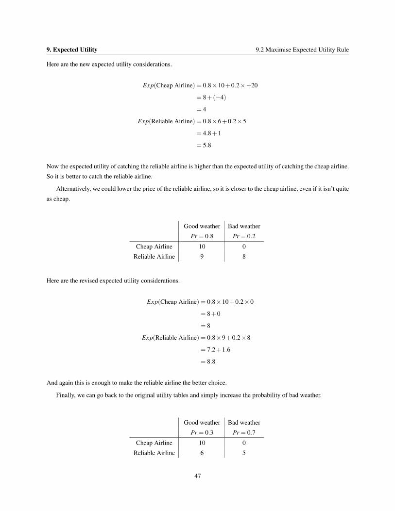
9. Expected Utility 9.2 Maximise Expected Utility Rule

Here are the new expected utility considerations.

Exp(Cheap Airline) = 0.8×10+0.2×−20

= 8+(−4)

= 4


= 4.8+1

= 5.8

Now the expected utility of catching the reliable airline is higher than the expected utility of catching the cheap airline.

So it is better to catch the reliable airline.

Alternatively, we could lower the price of the reliable airline, so it is closer to the cheap airline, even if it isn’t quite

as cheap.


Pr = 0.8 Pr = 0.2

Cheap Airline 10 0


Here are the revised expected utility considerations.


= 8+0

= 8


= 7.2+1.6

= 8.8

And again this is enough to make the reliable airline the better choice.

Finally, we can go back to the original utility tables and simply increase the probability of bad weather.


Pr = 0.3 Pr = 0.7

Cheap Airline 10 0


47

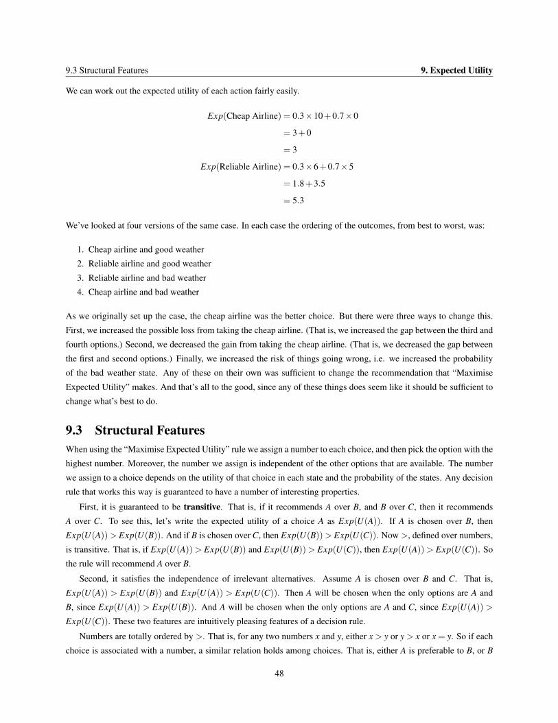
9.3 Structural Features 9. Expected Utility

We can work out the expected utility of each action fairly easily.


= 3+0

= 3


= 1.8+3.5

= 5.3

We’ve looked at four versions of the same case. In each case the ordering of the outcomes, from best to worst, was:

1. Cheap airline and good weather

2. Reliable airline and good weather

3. Reliable airline and bad weather

4. Cheap airline and bad weather

As we originally set up the case, the cheap airline was the better choice. But there were three ways to change this.

First, we increased the possible loss from taking the cheap airline. (That is, we increased the gap between the third and

fourth options.) Second, we decreased the gain from taking the cheap airline. (That is, we decreased the gap between

the first and second options.) Finally, we increased the risk of things going wrong, i.e. we increased the probability

of the bad weather state. Any of these on their own was sufficient to change the recommendation that “Maximise

Expected Utility” makes. And that’s all to the good, since any of these things does seem like it should be sufficient to

change what’s best to do.

9.3 Structural FeaturesWhen using the “Maximise Expected Utility” rule we assign a number to each choice, and then pick the option with the

highest number. Moreover, the number we assign is independent of the other options that are available. The number

we assign to a choice depends on the utility of that choice in each state and the probability of the states. Any decision

rule that works this way is guaranteed to have a number of interesting properties.

First, it is guaranteed to be transitive. That is, if it recommends A over B, and B over C, then it recommends

A over C. To see this, let’s write the expected utility of a choice A as Exp(U(A)). If A is chosen over B, then

Exp(U(A)) > Exp(U(B)). And if B is chosen over C, then Exp(U(B)) > Exp(U(C)). Now >, defined over numbers,

is transitive. That is, if Exp(U(A)) > Exp(U(B)) and Exp(U(B)) > Exp(U(C)), then Exp(U(A)) > Exp(U(C)). So

the rule will recommend A over B.

Second, it satisfies the independence of irrelevant alternatives. Assume A is chosen over B and C. That is,

Exp(U(A)) > Exp(U(B)) and Exp(U(A)) > Exp(U(C)). Then A will be chosen when the only options are A and

B, since Exp(U(A)) > Exp(U(B)). And A will be chosen when the only options are A and C, since Exp(U(A)) >

Exp(U(C)). These two features are intuitively pleasing features of a decision rule.

Numbers are totally ordered by >. That is, for any two numbers x and y, either x > y or y > x or x = y. So if each

choice is associated with a number, a similar relation holds among choices. That is, either A is preferable to B, or B

48

9. Expected Utility 9.3 Structural Features

is preferable to A, or they are equally preferable. We’ll come back in later chapters to the question of whether this is

plausible.

Expected utility maximisation never recommends choosing dominated options. Assume that A dominates B. For

each state Si, write utility of A in Si as U(A|Si). Then dominance means that for all i, U(A|Si) > U(B|Si). Now

Exp(U(A)) and Exp(U(B)) are given by the following formulae. (In what follows n is the number of possible states.)

Exp(A) = Pr(S1)U(A|S1)+Pr(S2)U(A|S2)+ ...+Pr(Sn)U(A|Sn)

Exp(B) = Pr(S1)U(B|S1)+Pr(S2)U(B|S2)+ ...+Pr(Sn)U(B|Sn)

Note that the two values are each the sum of n terms. Note also that, given dominance, each term on the top row is

at least as great as than the term immediately below it on the second row. (This follows from the fact that U(A|Si) >

U(B|Si) and the fact that Pr(Si) ≥ 0.) Moreover, at least one of the terms on the top row is greater than the term

immediately below it. (This follows from the fact that U(A|Si) >U(B|Si) and the fact that for at least one i, Pr(Si) > 0.

That in turn has to be true because if Pr(Si) = 0 for each i, then Pr(S1∨S2∨ ...∨Sn) = 0. But S1∨S2∨ ...∨Sn has to

be true.) So Exp(A) has to be greater than Exp(B). So if A dominates B, it has a higher expected utility.

49

9.3 Structural Features 9. Expected Utility

50

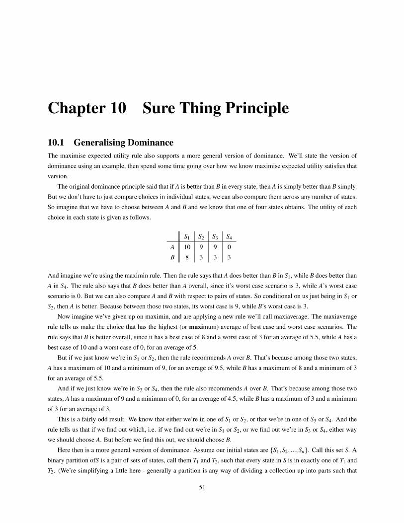
Chapter 10 Sure Thing Principle

10.1 Generalising DominanceThe maximise expected utility rule also supports a more general version of dominance. We’ll state the version of

dominance using an example, then spend some time going over how we know maximise expected utility satisfies that

version.

The original dominance principle said that if A is better than B in every state, then A is simply better than B simply.

But we don’t have to just compare choices in individual states, we can also compare them across any number of states.

So imagine that we have to choose between A and B and we know that one of four states obtains. The utility of each

choice in each state is given as follows.

S1 S2 S3 S4

A 10 9 9 0

B 8 3 3 3

And imagine we’re using the maximin rule. Then the rule says that A does better than B in S1, while B does better than

A in S4. The rule also says that B does better than A overall, since it’s worst case scenario is 3, while A’s worst case

scenario is 0. But we can also compare A and B with respect to pairs of states. So conditional on us just being in S1 or

S2, then A is better. Because between those two states, its worst case is 9, while B’s worst case is 3.

Now imagine we’ve given up on maximin, and are applying a new rule we’ll call maxiaverage. The maxiaverage

rule tells us make the choice that has the highest (or maximum) average of best case and worst case scenarios. The

rule says that B is better overall, since it has a best case of 8 and a worst case of 3 for an average of 5.5, while A has a

best case of 10 and a worst case of 0, for an average of 5.

But if we just know we’re in S1 or S2, then the rule recommends A over B. That’s because among those two states,

A has a maximum of 10 and a minimum of 9, for an average of 9.5, while B has a maximum of 8 and a minimum of 3

for an average of 5.5.

And if we just know we’re in S3 or S4, then the rule also recommends A over B. That’s because among those two

states, A has a maximum of 9 and a minimum of 0, for an average of 4.5, while B has a maximum of 3 and a minimum

of 3 for an average of 3.

This is a fairly odd result. We know that either we’re in one of S1 or S2, or that we’re in one of S3 or S4. And the

rule tells us that if we find out which, i.e. if we find out we’re in S1 or S2, or we find out we’re in S3 or S4, either way

we should choose A. But before we find this out, we should choose B.

Here then is a more general version of dominance. Assume our initial states are {S1,S2, ...,Sn}. Call this set S. A

binary partition ofS is a pair of sets of states, call them T1 and T2, such that every state in S is in exactly one of T1 and

T2. (We’re simplifying a little here - generally a partition is any way of dividing a collection up into parts such that

51

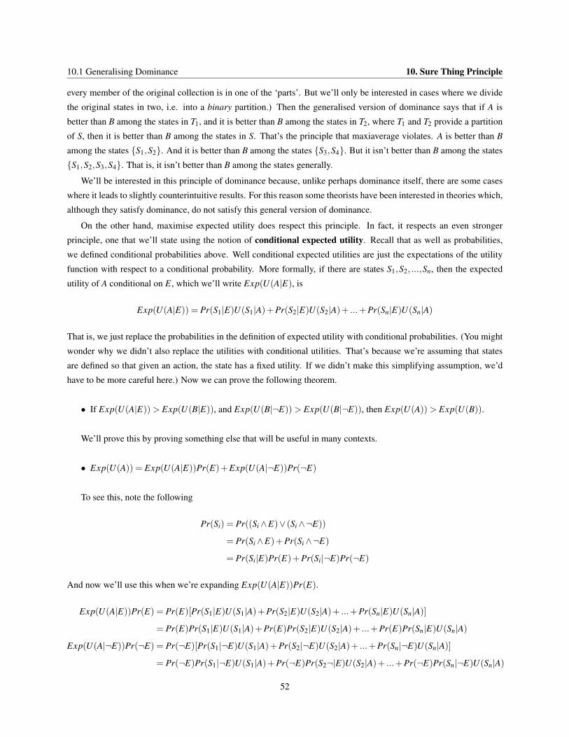
10.1 Generalising Dominance 10. Sure Thing Principle

every member of the original collection is in one of the ‘parts’. But we’ll only be interested in cases where we divide

the original states in two, i.e. into a binary partition.) Then the generalised version of dominance says that if A is

better than B among the states in T1, and it is better than B among the states in T2, where T1 and T2 provide a partition

of S, then it is better than B among the states in S. That’s the principle that maxiaverage violates. A is better than B

among the states {S1,S2}. And it is better than B among the states {S3,S4}. But it isn’t better than B among the states

{S1,S2,S3,S4}. That is, it isn’t better than B among the states generally.

We’ll be interested in this principle of dominance because, unlike perhaps dominance itself, there are some cases

where it leads to slightly counterintuitive results. For this reason some theorists have been interested in theories which,

although they satisfy dominance, do not satisfy this general version of dominance.

On the other hand, maximise expected utility does respect this principle. In fact, it respects an even stronger

principle, one that we’ll state using the notion of conditional expected utility. Recall that as well as probabilities,

we defined conditional probabilities above. Well conditional expected utilities are just the expectations of the utility

function with respect to a conditional probability. More formally, if there are states S1,S2, ...,Sn, then the expected

utility of A conditional on E, which we’ll write Exp(U(A|E), is

Exp(U(A|E)) = Pr(S1|E)U(S1|A)+Pr(S2|E)U(S2|A)+ ...+Pr(Sn|E)U(Sn|A)

That is, we just replace the probabilities in the definition of expected utility with conditional probabilities. (You might

wonder why we didn’t also replace the utilities with conditional utilities. That’s because we’re assuming that states

are defined so that given an action, the state has a fixed utility. If we didn’t make this simplifying assumption, we’d

have to be more careful here.) Now we can prove the following theorem.

• If Exp(U(A|E)) > Exp(U(B|E)), and Exp(U(B|¬E)) > Exp(U(B|¬E)), then Exp(U(A)) > Exp(U(B)).

We’ll prove this by proving something else that will be useful in many contexts.

• Exp(U(A)) = Exp(U(A|E))Pr(E)+Exp(U(A|¬E))Pr(¬E)

To see this, note the following

Pr(Si) = Pr((Si∧E)∨ (Si∧¬E))

= Pr(Si∧E)+Pr(Si∧¬E)

= Pr(Si|E)Pr(E)+Pr(Si|¬E)Pr(¬E)

And now we’ll use this when we’re expanding Exp(U(A|E))Pr(E).

Exp(U(A|E))Pr(E) = Pr(E)[Pr(S1|E)U(S1|A)+Pr(S2|E)U(S2|A)+ ...+Pr(Sn|E)U(Sn|A)]

= Pr(E)Pr(S1|E)U(S1|A)+Pr(E)Pr(S2|E)U(S2|A)+ ...+Pr(E)Pr(Sn|E)U(Sn|A)

Exp(U(A|¬E))Pr(¬E) = Pr(¬E)[Pr(S1|¬E)U(S1|A)+Pr(S2|¬E)U(S2|A)+ ...+Pr(Sn|¬E)U(Sn|A)]

= Pr(¬E)Pr(S1|¬E)U(S1|A)+Pr(¬E)Pr(S2¬|E)U(S2|A)+ ...+Pr(¬E)Pr(Sn|¬E)U(Sn|A)

52

10. Sure Thing Principle 10.2 Sure Thing Principle

Putting those two together, we get

Exp(U(A|E))Pr(E)+Exp(U(A|¬E))Pr(¬E)

= Pr(E)Pr(S1|E)U(S1|A)+ ...+Pr(E)Pr(Sn|E)U(Sn|A)+

+Pr(¬E)Pr(S1|¬E)U(S1|A)+ ...+Pr(¬E)Pr(Sn|¬E)U(Sn|A)

= (Pr(E)Pr(S1|E)+Pr(¬E)Pr(S1|¬E))U(S1|A)+ ...+(Pr(E)Pr(Sn|E)+Pr(¬E)Pr(Sn|¬E))U(Sn|A)

= Pr(S1)U(S1|A)+Pr(S2)U(S2|A)+ ...Pr(Sn)U(Sn|A)

= Exp(U(A))

Now if Exp(U(A|E)) > Exp(U(B|E)), and Exp(U(B|¬E)) > Exp(U(B|¬E)), then the following two inequalities

hold.

Exp(U(A|E))Pr(E)≥ Exp(U(B|E))Pr(E)

Exp(U(A|¬E))Pr(¬E)≥ Exp(U(B|¬E))Pr(¬E)

In each case we have equality only if the probability in question (Pr(E) in the first line, Pr(¬E) in the second) is zero.

Since not both Pr(E) and Pr(¬E) are zero, one of those is a strict inequality. (That is, the left hand side is greater

than, not merely greater than or equal to, the right hand side.) So adding up the two lines, and using the fact that in

one case we have a strict inequality, we get

Exp(U(A|E))Pr(E)+Exp(U(A|¬E))Pr(¬E)≥ Exp(U(B|E))Pr(E)+Exp(U(B|¬E))Pr(¬E)

i.e. Exp(U(A)) > Exp(U(B))

That is, if A is better than B conditional on E, and it is better than B conditional on ¬E, then it is simply better than B.

10.2 Sure Thing PrincipleThe result we just proved is very similar to a famous principle of decision theory, the Sure Thing Principle. The Sure

Thing Principle is usually stated in terms of one option being at least as good as another, rather than one option being

better than another, as follows.

Sure Thing Principle If AE � BE and A¬E � B¬E, then A� B.

The terminology there could use some spelling out. By A � B we mean that A is preferred to B. By A � B we mean

that A is regarded as at least as good as B. The relation between � and � is like the relation between ¿ and ≥. In each

case the line at the bottom means that we’re allowing equality between the values on either side.

The odd thing here is using AE � BE rather than something that’s explicitly conditional. We should read the terms

on each side of the inequality sign as conjunctions. It means that A and E is regarded as at least as good an outcome

as B and E. But that sounds like something that’s true just in case the agent prefers A to B conditional on E obtaining.

So we can use preferences over conjunctions like AE as proxy for conditional preferences.

So we can read the Sure Thing Principle as saying that if A is at least as good as B conditional on E, and conditional

on ¬E, then it really is at least as good as B. Again, this looks fairly plausible in the abstract, though we’ll soon see

some reasons to worry about it.

53

10.3 Allais Paradox 10. Sure Thing Principle

Expected Utility maximisation satisfies the Sure Thing Principle. I won’t go over the proof here because it’s really

just the same as the proof from the previous section with > replaced by ≥ in a lot of places. But if we regard the Sure

Thing Principle as a plausible principle of decision making, then it is a good feature of Expected Utility maximisation

that it satisfies it.

It is tempting to think of the Sure Thing Principle as a generalisation of a principle of logical implication we all

learned in propositional logic. The principle in question said that from X → Z, and Y → Z, and X ∨Y , we can infer C.

If we let Z be that A is better than B, let X be E, and Y be ¬E, it looks like we have all the premises, and the reasoning

looks intuitively right. But this analogy is misleading for two reasons.

First, for technical reasons we can’t get into in depth here, preferring A to B conditional on E isn’t the same as it

being true that if E is true you prefer A to B. To see some problems with this, think about cases where you don’t know

E is true, and A is something quite horrible that mitigates the effects of the unpleasant E. In this case you do prefer

AE to BE, and E is true, but you don’t prefer A to B. But we’ll set this question, which is largely a logical question

about the nature of conditionals, to one side.

The bigger problem is that the analogy with logic would suggest that the following generalisation of the Sure Thing

Principle will hold.

Disjunction Principle If AE1 � BE1 and AE2 � BE2, and Pr(E1∨E2) = 1 then A� B.

But this “Disjunction Principle” seems no good in cases like the following. I’m going to toss two coins. Let p be the

proposition that they will land differently, i.e. one heads and one tails. I offer you a bet that pays you $2 if p, and costs

you $3 if ¬p. This looks like a bad bet, since Pr(p) = 0.5, and losing $3 is worse than gaining $2. But consider the

following argument.

Let E1 be that at least one of the coins landing heads. It isn’t too hard to show that Pr(p|E1) = 23 . So conditional

on E1, the expected return of the bet is 23 ×2− 1

3 ×3 = 43 −1 = 1

3 . That’s a positive return. So if we let A be taking the

bet, and B be declining the bet, then conditional on E1, A is better than B, because the expected return is positive.

Let E2 be that at least one of the coins landing tails. It isn’t too hard to show that Pr(p|E1) = 23 . So conditional on

E2, the expected return of the bet is 23 ×2− 1

3 ×3 = 43 −1 = 1

3 . That’s a positive return. So if we let A be taking the

bet, and B be declining the bet, then conditional on E2, A is better than B, because the expected return is positive.

Now if E1 fails, then both of the coins lands tails. That means that at least one of the coins lands tails. That means

that E2 is true. So if E1 fails E2 is true. So one of E1 and E2 has to be true, i.e. Pr(E1∨E2) = 1. And AE1 � BE1 and

AE2 � BE2. Indeed AE1 � BE1 and AE2 � BE2. But B� A. So the disjunction principle isn’t in general true.

It’s a deep philosophical question how seriously we should worry about this. If the Sure Thing Principle isn’t any

more plausible intuitively than the Disjunction Principle, and the Disjunction Principle seems false, does that mean

we should be sceptical of the Sure Thing Principle? As I said, that’s a very hard question, and it’s one we’ll return to

a few times in what follows.

10.3 Allais ParadoxThe Sure Thing Principle is one of the more controversial principles in decision theory because there seem to be cases

where it gives the wrong answer. The most famous of these is the Allais paradox, first discovered by the French

economist (and Nobel Laureate) Maurice Allais. In this paradox, the subject is first offered the following choice

between A and B. The results of their choice will depend on the drawing of a coloured ball from an urn. The urn

54

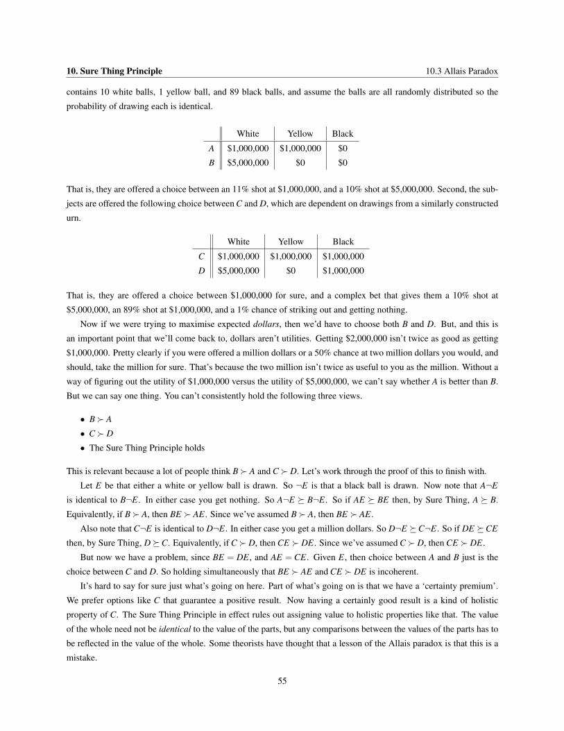
10. Sure Thing Principle 10.3 Allais Paradox

contains 10 white balls, 1 yellow ball, and 89 black balls, and assume the balls are all randomly distributed so the

probability of drawing each is identical.

White Yellow Black

A $1,000,000 $1,000,000 $0

B $5,000,000 $0 $0

That is, they are offered a choice between an 11% shot at $1,000,000, and a 10% shot at $5,000,000. Second, the sub-

jects are offered the following choice between C and D, which are dependent on drawings from a similarly constructed

urn.

White Yellow Black

C $1,000,000 $1,000,000 $1,000,000

D $5,000,000 $0 $1,000,000

That is, they are offered a choice between $1,000,000 for sure, and a complex bet that gives them a 10% shot at

$5,000,000, an 89% shot at $1,000,000, and a 1% chance of striking out and getting nothing.

Now if we were trying to maximise expected dollars, then we’d have to choose both B and D. But, and this is

an important point that we’ll come back to, dollars aren’t utilities. Getting $2,000,000 isn’t twice as good as getting

$1,000,000. Pretty clearly if you were offered a million dollars or a 50% chance at two million dollars you would, and

should, take the million for sure. That’s because the two million isn’t twice as useful to you as the million. Without a

way of figuring out the utility of $1,000,000 versus the utility of $5,000,000, we can’t say whether A is better than B.

But we can say one thing. You can’t consistently hold the following three views.

• B� A

• C � D

• The Sure Thing Principle holds

This is relevant because a lot of people think B� A and C � D. Let’s work through the proof of this to finish with.

Let E be that either a white or yellow ball is drawn. So ¬E is that a black ball is drawn. Now note that A¬E

is identical to B¬E. In either case you get nothing. So A¬E � B¬E. So if AE � BE then, by Sure Thing, A � B.

Equivalently, if B� A, then BE � AE. Since we’ve assumed B� A, then BE � AE.

Also note that C¬E is identical to D¬E. In either case you get a million dollars. So D¬E �C¬E. So if DE �CE

then, by Sure Thing, D�C. Equivalently, if C � D, then CE � DE. Since we’ve assumed C � D, then CE � DE.

But now we have a problem, since BE = DE, and AE = CE. Given E, then choice between A and B just is the

choice between C and D. So holding simultaneously that BE � AE and CE � DE is incoherent.

It’s hard to say for sure just what’s going on here. Part of what’s going on is that we have a ‘certainty premium’.

We prefer options like C that guarantee a positive result. Now having a certainly good result is a kind of holistic

property of C. The Sure Thing Principle in effect rules out assigning value to holistic properties like that. The value

of the whole need not be identical to the value of the parts, but any comparisons between the values of the parts has to

be reflected in the value of the whole. Some theorists have thought that a lesson of the Allais paradox is that this is a

mistake.

55

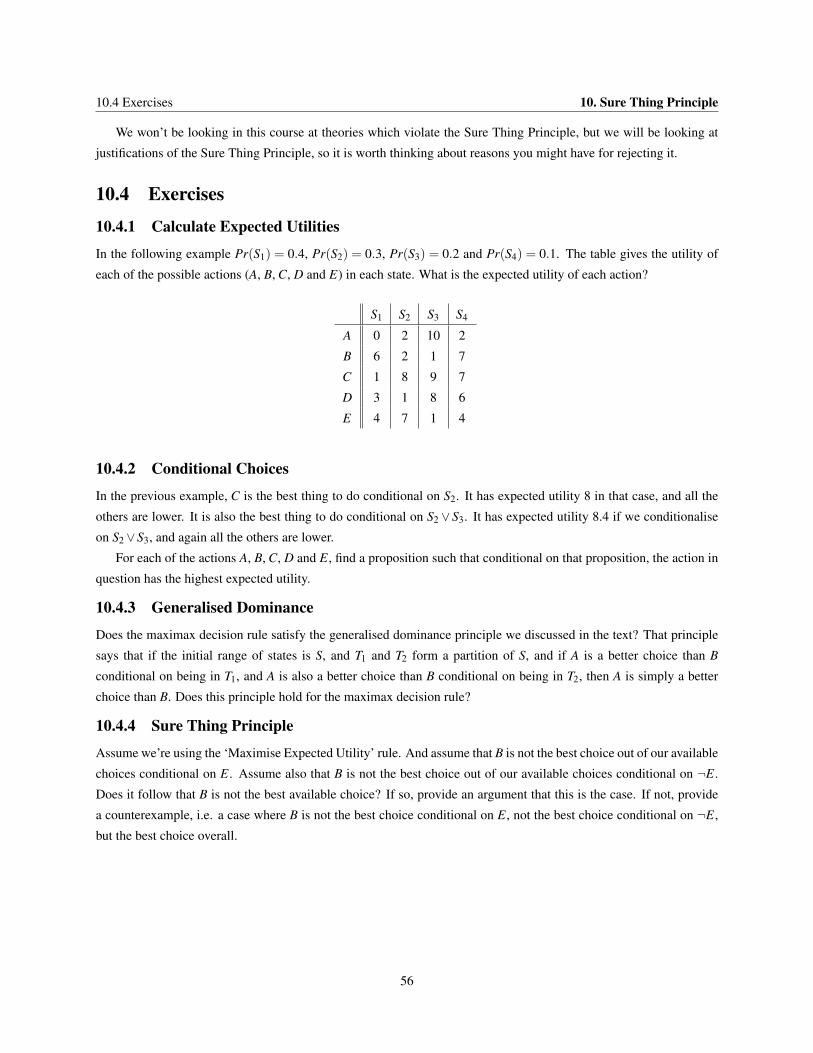
10.4 Exercises 10. Sure Thing Principle

We won’t be looking in this course at theories which violate the Sure Thing Principle, but we will be looking at

justifications of the Sure Thing Principle, so it is worth thinking about reasons you might have for rejecting it.

10.4 Exercises

10.4.1 Calculate Expected Utilities

In the following example Pr(S1) = 0.4, Pr(S2) = 0.3, Pr(S3) = 0.2 and Pr(S4) = 0.1. The table gives the utility of

each of the possible actions (A, B, C, D and E) in each state. What is the expected utility of each action?

S1 S2 S3 S4

A 0 2 10 2

B 6 2 1 7

C 1 8 9 7

D 3 1 8 6

E 4 7 1 4

10.4.2 Conditional Choices

In the previous example, C is the best thing to do conditional on S2. It has expected utility 8 in that case, and all the

others are lower. It is also the best thing to do conditional on S2 ∨ S3. It has expected utility 8.4 if we conditionalise

on S2∨S3, and again all the others are lower.

For each of the actions A, B, C, D and E, find a proposition such that conditional on that proposition, the action in

question has the highest expected utility.

10.4.3 Generalised Dominance

Does the maximax decision rule satisfy the generalised dominance principle we discussed in the text? That principle

says that if the initial range of states is S, and T1 and T2 form a partition of S, and if A is a better choice than B

conditional on being in T1, and A is also a better choice than B conditional on being in T2, then A is simply a better

choice than B. Does this principle hold for the maximax decision rule?

10.4.4 Sure Thing Principle

Assume we’re using the ‘Maximise Expected Utility’ rule. And assume that B is not the best choice out of our available

choices conditional on E. Assume also that B is not the best choice out of our available choices conditional on ¬E.

Does it follow that B is not the best available choice? If so, provide an argument that this is the case. If not, provide

a counterexample, i.e. a case where B is not the best choice conditional on E, not the best choice conditional on ¬E,

but the best choice overall.

56

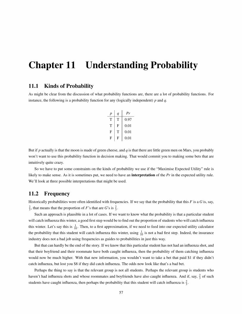
Chapter 11 Understanding Probability

11.1 Kinds of ProbabilityAs might be clear from the discussion of what probability functions are, there are a lot of probability functions. For

instance, the following is a probability function for any (logically independent) p and q.

p q Pr

T T 0.97

T F 0.01

F T 0.01

F F 0.01

But if p actually is that the moon is made of green cheese, and q is that there are little green men on Mars, you probably

won’t want to use this probability function in decision making. That would commit you to making some bets that are

intuitively quite crazy.

So we have to put some constraints on the kinds of probability we use if the “Maximise Expected Utility” rule is

likely to make sense. As it is sometimes put, we need to have an interpretation of the Pr in the expected utility rule.

We’ll look at three possible interpretations that might be used.

11.2 FrequencyHistorically probabilities were often identified with frequencies. If we say that the probability that this F is a G is, say,23 , that means that the proportion of F’s that are G’s is 2

3 .

Such an approach is plausible in a lot of cases. If we want to know what the probability is that a particular student

will catch influenza this winter, a good first step would be to find out the proportion of students who will catch influenza

this winter. Let’s say this is 110 . Then, to a first approximation, if we need to feed into our expected utility calculator

the probability that this student will catch influenza this winter, using 110 is not a bad first step. Indeed, the insurance

industry does not a bad job using frequencies as guides to probabilities in just this way.

But that can hardly be the end of the story. If we know that this particular student has not had an influenza shot, and

that their boyfriend and their roommate have both caught influenza, then the probability of them catching influenza

would now be much higher. With that new information, you wouldn’t want to take a bet that paid $1 if they didn’t

catch influenza, but lost you $8 if they did catch influenza. The odds now look like that’s a bad bet.

Perhaps the thing to say is that the relevant group is not all students. Perhaps the relevant group is students who

haven’t had influenza shots and whose roommates and boyfriends have also caught influenza. And if, say, 23 of such

students have caught influenza, then perhaps the probability that this student will catch influenza is 23 .

57

11.3 Degrees of Belief 11. Understanding Probability

You might be able to see where this story is going by now. We can always imagine more details that will make that

number look inappropriate as well. Perhaps the student in question is spending most of the winter doing field work in

South America, so they have little chance to catch influenza from their infected friends. And now the probability should

be lower. Or perhaps we can imagine that they have a genetic predisposition to catch influenza, so the probability

should be higher. There is always more information that could be relevant.

The problem for using frequencies as probabilities then is that there could always be more precise information that

is relevant to the probability. Every time we find that the person in question isn’t merely an F (a student, say), but is a

particular kind of F (a student who hasn’t had an influenza shot, whose close contacts are infected, who has a genetic

predisposition to influenza), we want to know the proportion not of F’s who are G’s, but the proportion of the more

narrowly defined class who are G’s. But eventually this will leave us with no useful probabilities at all, because we’ll

have found a way of describing the student in question such that they are the only person in history who satisfies this

description.

This is hardly a merely theoretical concern. If we are interested in the probability that a particular bank will

go bankrupt, or that a particular Presidential candidate will win election, it isn’t too hard to come up with a list of

characteristics of the bank or candidate in question in such a way that they are the only one in history to meet that

description. So the frequency that such banks will go bankrupt is either 1 (1 out of 1 go bankrupt) or 0 (0 out of 1 do).

But those aren’t particularly useful probabilities. So we should look elsewhere for an interpretation of the Pr that goes

into our definition of expected utility.

In the literature there are two objections to using frequencies as probabilities that seem related to the argument

we’re looking at here.

One of these is the Reference Class Problem. This is the problem that if we’re interested in the probability that a

particular person is G, then the frequency of G-hood amongst the different classes the person is in might differ.

The other is the Single Case Problem. This is the problem that we’re often interested in one-off events, like bank

failures, elections, wars etc, that don’t naturally fit into any natural broader category.

I think the reflections here support the idea that these are two sides of a serious problem for the view that prob-

abilities are frequencies. In general, there actually is a natural solution to the Reference Class Problem. We look

to the most narrowly drawn reference class we have available. So if we’re interested in whether a particular person

will survive for 30 years, and we know they are a 52 year old man who smokes, we want to look not to the survival

frequencies of people in general, or men in general, or 52 year old men in general, but 52 year old male smokers.

Perhaps by looking at cases like this, we can convince ourselves that there is a natural solution to the Reference

Class Problem. But the solution makes the Single Case Problem come about. Pretty much anything that we care about

is distinct in some way or another. That’s to say, if we look closely we’ll find that the most natural reference class for it

just contains that one thing. That’s to say, it’s a single case in some respect. And one-off events don’t have interesting

frequencies. So frequencies aren’t what we should be looking to as probabilities.

11.3 Degrees of BeliefIn response to these worries, a lot of philosophers and statisticians started thinking of probability in purely subjective

terms. The probability of a proposition p is just how confident the agent is that p will obtain. This level of confidence

is the agent’s degree of belief that p will obtain.

Now it isn’t altogether to measure degrees of belief. I might be fairly confident that my baseball team will win

58

11. Understanding Probability 11.3 Degrees of Belief

tonight, and more confident that they’ll win at least one of the next three games, and less confident that they’ll win all

of their next three games, but how could we measure numerically each of those strengths. Remember that probabilities

are numbers. So if we’re going to identify probabilities with degrees of belief, we have to have a way to convert

strengths of confidence to numbers.

The core idea about how to do this uses the very decision theory that we’re looking for input to. I’ll run through

a rough version of how the measurement works; we’ll be refining this quite a bit as the course goes on. Imagine you

have a chance to buy a ticket that pays $1 if p is true. How much, in dollars, is the most would you pay for this? Well,

it seems that how much you should pay for this is the probability of p. Let’s see why this is true. (Assume in what

follows that the utility of each action is given by how many dollars you get from the action; this is the simplifying

assumption we’re making.) If you pay $Pr(p) for the ticket, then you’ve performed some action (call it A) that has the

following payout structure.

U(A) =

1−Pr(p) if p,

−Pr(p) if ¬p.

So the expected value of U(A) is

Exp(U(A)) = Pr(p)U(Ap)+Pr(¬p)U(A¬p)

= Pr(p)(1−Pr(p))+Pr(¬p)U(A¬p)

= Pr(p)(1−Pr(p))+(1−Pr(p))(−Pr(p))

= Pr(p)(1−Pr(p))− (1−Pr(p))(Pr(p))

= 0

So if you pay $Pr(p) for the bet, your expected return is exactly 0. Obviously if you pay more, you’re worse off,

and if you pay less, you’re better off. $Pr(p) is the break even point, so that’s the fair price for the bet.

And that’s how we measure degrees of belief. We look at the agent’s ‘fair price’ for a bet that returns $1 if p.

(Alternatively, we look at the maximum they’ll pay for such a bet.) And that’s they’re degree of belief that p. If we’re

taking probabilities to be degrees of belief, if we are (as it is sometimes put) interpreting probability subjectively, then

that’s the probability of p.

This might look suspiciously circular. The expected utility rule was meant to give us guidance as to how we should

make decisions. But the rule needed a probability as an input. And now we’re taking that probability to not only be a

subjective state of the agent, but a subjective state that is revealed in virtue of the agent’s own decisions. Something

seems odd here.

Perhaps we can make it look even odder. Let p be some proposition that might be true and might be false, and

assume that the agent’s choice is to take or decline a bet on p that has some chance of winning and some chance of

losing. Then if the agent takes the bet, that’s a sign that their degree of belief in p was higher than the odds of the bet

on p, so therefore they are increasing their expected utility by taking the bet, so they are doing the right thing. On the

other hand, if they decline the bet, that’s a sign that their degree of belief in p was lower than the odds of the bet on

p, so therefore they are increasing their expected utility by taking the bet, so they are doing the right thing. So either

way, they do the right thing. But a rule that says they did the right thing whatever they do isn’t much of a rule.

59

11.3 Degrees of Belief 11. Understanding Probability

There are two important responses to this, which are related to one another. The first is that although the rule does

(more or less) put no restrictions at all on what you do when faced with a single choice, it can put quite firm constraints

on your sets of choices when you have to make multiple decisions. The second is that the rule should be thought of as

a procedural rather than substantive rule of rationality. We’ll look at these more closely.

If we take probabilities to be subjective probabilities, i.e. degrees of belief, then the maximise expected utility rule

turns out to be something like a consistency constraint. Compare it to a rule like Have Consistent Beliefs. As long as

we’re talking about logically contingent matters, this doesn’t put any constraint at all on what you do when faced with

a single question of whether to believe p or ¬p. But it does put constraints on what further beliefs you can have once

you believe p. For instance, you can’t now believe ¬p.

The maximise expected utility rule is like this. Indeed we already saw this in the Allais paradox. The rule, far from

being empty, rules out the pair of choices that many people intuitively think is best. So if the objection is that the rule

has no teeth, that objection can’t hold up.

We can see this too in simpler cases. Let’s say I offer the agent a ticket that pays $1 if p, and she pays 60c for it.

So her degree of belief in p must be at least 0.6. Then I offer her a ticket that pays $1 if ¬p, and she pays 60c for it

too. So her degree of belief in ¬p must be at least 0.6. But, and here’s the constraint, we think degrees of belief have

to be probabilities. And if Pr(p) > 0.6, then Pr(¬p) < 0.4. So if Pr(¬p) > 0.6, we have an inconsistency. That’s bad,

and it’s the kind of badness it is the job of the theory to rule out.

One way to think about the expected utility rule is to compare it to norms of means-end rationality. At times

when we’re thinking about what someone should do, we really focus on what the best means is to their preferred end.

So we might say If you want to go to Harlem, you should take the A train, without it even being a relevant question

whether they should, in the circumstances, want to go to Harlem.

The point being made here is quite striking when we consider people with manifestly crazy beliefs. If we’re just

focussing on means to an end, then we might look at someone who, say, wants to crawl from the southern tip of

Broadway to its northern tip. And we’ll say “You should get some kneepads so you don’t scrape your knees, and you

should take lots of water, and you should catch the 1 train down to near to where Broadway starts, etc.” But if we’re

not just offering procedural advice, but are taking a more substantive look at their position, we’ll say “You should

come up with a better idea about what to do, because that’s an absolutely crazy thing to want.”

As we’ll see, the combination of the maximise expected utility rule with the use of degrees of belief as probabilities

leads to a similar set of judgments. On the one hand, it is a very good guide to procedural questions. But it leaves

some substantive questions worryingly unanswered. Next time we’ll come back to this distinction, and see if there’s a

better way to think about probability.

60

Chapter 12 Objective Probabilities

12.1 Credences and NormsWe ended last time with looking at the idea that the probabilities in expected utility calculations should be subjective.

As it is sometimes put, they should be degrees of belief. Or, as it is also sometimes put, they should be credences. We

noted that under this interpretation, the maximise expected utility rule doesn’t put any constraints on certain simple

decisions. That’s because we use the rule to calculate what credences are, and then use the very same credences to

say what the rule requires. But the rule isn’t useless. It puts constraints, often sharp constraints, on sets of decisions.

In this respect it is more like the rule Have Consistent Beliefs than like the rule Believe What’s True, or Believe What

Your Evidence Supports. And we compared it to procedural, as opposed to substantive norms.

What’s left from all that are two large questions.

• Do we get the right procedural/consistency constraints from the expected utility rule? In particular (a) should

credences be probabilities, and (b) should we make complex decisions by the expected utility rule? We’ll look

a bit in what follows at each of these questions.

• Is a purely procedural constraint all we’re looking for in a decision theory?

And intuitively the answer to the second question is No. Let’s consider a particular case. Alex is very confident

that the Kansas City Royals will win baseball’s World Series next year. In fact, Alex’s credence in this is 0.9, very

close to 1. Unfortunately, there is little reason for this confidence. Kansas City has been one of the worst teams in

baseball for many years, the players they have next year will be largely the same as the players they had when doing

poorly this year, and many other teams have players who have performed much much better. Even if Kansas City were

a good team, there are 30 teams in baseball, and relatively random events play a big role in baseball, making it unwise

to be too confident that any one team will win.

Now, Alex is offered a bet that leads to a $1 win if Kansas City win the World Series, and a $1 loss if they do not.

The expected return of that bet, given Alex’s credences, is +80c. So should Alex make the bet?

Intuitively, Alex should not. It’s true that given Alex’s credences, the bet is a good one. But it’s also true that Alex

has crazy credences. Given more sensible credences, the bet has a negative expected return. So Alex should not make

the bet.

It’s worth stepping away from probabilities, expected values and the like to think about this in a simpler context.

Imagine a person has some crazy beliefs about what is an effective way to get some good end. And assume they, quite

properly, want that good end. In fact, however, acting on their crazy beliefs will be counterproductive; it will just make

things worse for everyone. And their evidence supports this. Should they act on their beliefs? Intuitively not. To be

sure, if they didn’t act on their beliefs, there would be some inconsistency between their beliefs and their actions. But

inconsistency isn’t the worst thing in the world. They should, instead, have different beliefs.

61

12.2 Evidential Probability 12. Objective Probabilities

Similarly Alex should have different credences in the case in question. The question, what should Alex do given

these credences, seems less interesting than the question, what should Alex do? And that’s what we’ll look at.

12.2 Evidential ProbabilityWe get a better sense of what an agent should do if we look not to what credences they have, but to what credences

they should have. Let’s try to formalise this as the credences they would have if they were perfectly rational.

Remember credences are still being measured by betting behaviour, but now it is betting behaviour under the

assumption of perfect rationality. So the probability of p is the highest price the agent would pay for a bet that pays $1

if p, if they were perfectly rational. The thing that should be done then is the thing that has the highest expected utility,

relative to this probability function. In the simple case where the choice is between taking and declining a bet, this

becomes a relatively boring theory - you should take the bet if you would take the bet if you were perfectly rational.

In the case of more complicated decisions, it becomes a much more substantive theory. (We’ll see examples of this in

later weeks.)

But actually we’ve said enough to give us two philosophical puzzles.

The first concerns whether there determinately is a thing that you would do if you were perfectly rational. Consider

a case where you have quite a bit of evidence for and against p. Different rational people will evaluate the evidence

in different ways. Some people will evaluate p as being more likely than not, and so take a bet at 50/50 odds on p.

Others will consider the evidence against p to be stronger, and hence decline a bet at 50/50 odds. It seems possible

that both sides in such a dispute could be perfectly rational.

The danger here is that if we define rational credences as the credences a perfectly rational person would have,

we might not have a precise definition. There may be many different credences that a perfectly rational person would

have. That’s bad news for a purported definition of rational credence.

The other concerns cases where p is about your own rationality. Let’s say p is the proposition that you are perfectly

rational. Then if you were perfectly rational, your credence in this would probably be quite high. But that’s not the

rational credence for you to have right now in p. You should be highly confident that you, like every other human

being on the planet, are susceptible to all kinds of failures of rationality. So it seems like a mistake in general to set

your credences to what they would be were you perfectly rational.

What seems better in general is to proportion your credences to the evidence. The rational credences are the ones

that best reflect the evidence you have in favour of various propositions. The idea here to to generate what’s usually

called an evidential probability. The probability of each proposition is a measure of how strongly it is supported by

the evidence.

That’s different from what a rational person would believe in two respects. For one thing, there is a fact about how

strongly the evidence supports p, even if different people might disagree about just how strongly that is. For another

thing, it isn’t true that the evidence supports that you are perfectly rational, even though you would believe that if you

were perfectly rational. So the two objections we just mentioned are not an issue here.

From now on then, when we talk about probability in the context of expected utility, we’ll talk about evidential

probabilities. There’s an issue, one we’ll return to later, about whether we can numerically measure strengths of

evidence. That is, there’s an issue about whether strengths of evidence are the right kind of thing to be put on a

numerical scale. Even if they are, there’s a tricky issue about how we can even guess what they are. I’m going to

cheat a little here. Despite the arguments above that evidential probabilities can’t be identified with betting odds of

62

12. Objective Probabilities 12.3 Objective Chances

perfectly rational agents, I’m going to assume that, unless we have reason to the contrary, those betting odds will be

our first approximation. So when we have to guess what the evidential probability of p is, we’ll start with what odds a

perfectly rational agent (with your evidence) would look for before betting on p.

12.3 Objective ChancesThere is another kind of probability that theorists are often interested in, one that plays a particularly important role

in modern physics. Classical physics was, or at least was thought to be, deterministic. Once the setup of the universe

at a time t was set, the laws of nature determined what would happen after t. Modern physics is not deterministic.

The laws don’t determine, say, how long it will take for an unstable particle to decay. Rather, all the laws say is that

the particle has such-and-such a chance of decaying in a certain time period. You might have heard references to the

half-life of different radioactive particles; this is the time in which the particle has a 12 probabiilty of decaying.

What are these probabilities that the scientists are talking about? Let’s call them ‘chances’ to give them a name.

So the question is, what is the status of chances. We know chances aren’t evidential probabilities. We know this for

three reasons.

One is that it is a tricky empirical question whether any event has any chance other than 0 or 1. It is now something

of a scientific consensus that some events are indeed chancy. But this relies on some careful scientific investigation. It

isn’t something we can tell from our armchairs. But we can tell from just thinking about decisions under uncertainty

that the evidential probability of some outcomes is between 0 and 1.

Another is that, as chances are often conceived, events taking place in the past do not, right now, have chances

other than 0 or 1. There might have been, at a point in the past, some intermediate chance of a particle decaying.

But if we’re now asking about whether a particle did decay or not in the last hour, then either it did decay, and its

chance is 0, or it did not decay, and its chance is 1. (I should note that not everyone thinks about chances in quite this

way, but it is a common way to think about them.) There are many events that took place in the past, however, whose

evidential probability is between 0 and 1. For instance, if we’re trying to meet up a friend, and hence trying to figure

out where the friend might have gone to, we’ll think about, and assign evidential probabilities to, various paths the

friend might have taken in the past. These thoughts won’t be thoughts about chances in the physicists’ sense; they’ll

be about evidential probabilities.

Finally, chances are objective. The evidential probability that p is true might be different for me than for you.

For instance, the evidence she has might make it quite likely for the juror that the suspect is guilty, even if he is not.

But the evidence the suspect has makes it extremely likely that he is innocent. Evidential probabilities differ between

different people. Chances do not. Someone might not know what the chance of a particular outcome is, but what they

are ignorant of is a matter of objective fact.

The upshot seems to be that chances are quite different things from evidential probabilities, and the best thing to

do is simply to take them to be distinct basic concepts.

12.4 The Principal Principle and Direct InferenceAlthough chances and evidential probabilities are distinct, it seems they stand in some close relation. If a trustworthy

physicist tells you that a particle has an 0.8 chance of decaying in the next hour, then it seems your credences should

be brought into line with what the physicists say. This idea has been dubbed the Principal Principle, because it is the

63

12.4 The Principal Principle and Direct Inference 12. Objective Probabilities

main principle linking chances and credences. If we use Pr for evidential probabilities, and Ch for objective chances

in the physicists’ sense, then the idea behind the principle is this.

Principal Principle Pr(p|Ch(p) = x) = x

That is, the probability of p, conditional on the chance of p being x, is x.

The Principal Principle may need to be qualified. If your evidence also includes that p, then even if the chance of

p is 0.8, perhaps your credence in p should be 1. After all, p is literally evident to you. But perhaps it is impossible

for p to be part of your evidence while its chance is less than 1. The examples given in the literature of how this could

come about are literally spectacular. Perhaps God tells you that p is true. Or perhaps a fortune teller with a crystal

ball sees that it is true. Or something equally bizarre happens. Any suggested exceptions to the principle have been

really outlandish. So whether the principle is true for all possible people in all possible worlds, it seems to hold for us

around here.

Chances, as the physicists think of them, are not frequencies. It might be possible to compute the theoretical

chance of a rare kind of particle not decaying over the course of an hour, even though the particle is so rare, and so

unstable, that no such particle has ever survived an hour. In that case the frequency of survival (i.e. the proportion of

all such particles that do actually survive an hour) is 0, but physical theory might tell us that the chance is greater than

0. Nevertheless chances are like frequencies in some respects.

One such respect is that chances are objective. Just as the chance of a particle decay is an objective fact, one that

we might or might not be aware of, the frequency of particle decay is also an objective fact that we might or might not

be aware of. Neither of these facts are in any way relative to the evidence of a particular agent, the way that evidential

probabilities are.

And just like chances, frequencies might seem to put a constraint on credences. Consider a case where the only

thing you know about a is that it is G. And you know that the frequency of F-hood among Gs is x. For instance, let a

be a person you’ve never met, G be the property of being a 74 year old male smoker, and F the property of surviving

10 more years. Then you might imagine knowing the survival statistics, but knowing nothing else about the person. In

that case, it’s very tempting to think the probability that a is F is x. In our example, we’d be identifying the probability

of this person surviving with the frequency of survival among people of the same type.

This inference from frequencies to probabilities is sometimes called “Direct Inference”. It is, at least on the

surface, a lot like the Principal Principle. But it is a fair bit more contentious. We’ll say a bit more about this once

we’ve looked about probabilities of events with infinite possibility spaces. But for now just note that it is really rather

rare that all we know about an individual can be summed up in one statistic like this. Even if the direct inference can

be philosophically justified (and I’m a little unsure that it can be) it will rarely be applicable. So it is less important

than the Principal Principle.

We’ll often invoke the Principal Principle tacitly in setting up problems. That is, when I want to set up a problem

where the probabilities of the various outcomes are given, I’ll often use objective chances to fix the probabilities of

various states. We’ll use the direct inference more sparingly, because it isn’t as clearly useful.

64

Chapter 13 Understanding Utility

13.1 Utility and WelfareSo far we’ve frequently talked about the utility of various outcomes. What we haven’t said a lot about is just what

it is that we’re measuring when we measure the utility of an outcomes. The intuitive idea is that utility is a measure

of welfare - having outcomes with higher utility if a matter of having a higher level of welfare. But this doesn’t

necessarily move the idea forward, because we’d like to know a bit more about what it is to have more welfare. There

are a number of ways we can frame the same question. We can talk about ‘well-being’ instead of welfare, or we can

talk about having a good life instead, or having a life that goes well. But the underlying philosophical question, what

makes it the case that a life has these features, remains more or less the same.

There are three primary kinds of theories of welfare in contemporary philosophy. These are

• Experience Based theories

• Objective List theories

• Preference Based theories

In decision theory, and indeed in economics, people usually focus on preference based theories. Indeed, the term

‘utility’ is sometimes used in such way that A has more utility than B just means that the agent prefers A to B. Indeed,

I’ve sometimes earlier moved back and forth previously between saying A has higher utility and saying A is preferred.

And the focus here (and in the next set of notes) will be on why people have moved to preference based accounts, and

technical challenges within those accounts. But we’ll start with the non-preference based accounts of welfare.

13.2 Experiences and WelfareOne tradition, tracing back at least to Jeremy Bentham, is to identify welfare with having good experiences. A person’s

welfare is high if they have lots of pleasures, and few pains. More generally, a person’s welfare is high if they have

good experiences.

Of course it is possible that a person might be increasing their welfare by having bad experiences at any one time.

They might be at work earning the money they need to finance activities that lead to good experiences later, or they

might just be looking for money to stave off bad experiences (starvation, lack of shelter) later. Or perhaps the bad

experiences, such as in strenuous exercise, are needed in order to be capable of later doing the things, e.g. engaging in

sporting activities, that produce good experiences. Either way, the point has to be that a person’s welfare is not simply

measured by what their experiences are like right now, but by what their experiences have been, are, and will be over

the course of their lives.

There is one well known objection to any such account - what Robert Nozick called the “experience machine”.

Imagine that a person is, in their sleep, kidnapped and wired up to a machine that produces in their brain the experiences

65

13.2 Experiences and Welfare 13. Understanding Utility

as of a fairly good life. The person still seems to be having good days filled with enjoyable experiences. And they

aren’t merely raw pleasurable sensations - the person is having experiences as of having rich fulfilling relationships

with the friends and family they have known and loved for years. But in fact the person is not in any contact with those

people, and for all the friends and family know, the person was kidnapped and killed. This continues for decades, until

the person has a peaceful death at an advanced age.

Has this person had a good life or a bad life? Many people think intuitively that they have had a bad life. Their

entire world has been based on an illusion. They haven’t really had fulfilling relationships, travelled to exciting places,

and so on. Instead they have been systematically deceived about the world. But on an experience based view of

welfare, they have had all of the goods you could want in life. Their experiences are just the experiences that a person

having a good life would have. So the experience based theorist is forced to say that they have had a good life, and

this seems mistaken.

Many philosophers find this a compelling objection to the experience based view of welfare. But many people are

not persuaded. So it’s worth thinking a little through some other puzzles for purely experience based views of welfare.

It’s easy enough to think about paradigmatic pains, or bad experiences. It isn’t too hard to come up with paradig-

matic good experiences, though perhaps there would be more disagreement about what experiences are paradigms of

the good than are paradigms of the bad. But many experiences are less easy to classify. Even simple experiences like

tickles might be good experiences for some, and bad experiences for others.

When we get to more complicated experiences, things are even more awkward for the experience based theorist.

Some people like listening to heavily distorted music, or watching horror movies, or drinking pineapple schnapps.

Other people, indeed most people, do not enjoy these things. The experience theory has a couple of choices here.

Either we can say that one group is wrong, and these things either do, or do not, raise one’s welfare. But this seems

implausible for all experiences. Perhaps at the fringes there are experiences people seek that nevertheless decrease

their welfare, but it seems strange to argue that the same experiences are good for everyone.

The other option is to say that there are really two experiences going on when you, say, listen to a kind of music

that some, but not all, people like. There is a ‘first-order’ experience of hearing the music. And there is a ‘second-

order’ experience, an experience of enjoying the experience of hearing the music. Perhaps this is right in some cases.

(Perhaps for horror movies, fans both feel horrified and have a pleasant reaction to being horrified, at least some of the

time.) But it seems wrong in general. If there is a food that I like and you dislike, that won’t usually be because I’ll

have a positive second-order experience, and you won’t have such a thing. Intuitively, the experience of, say, drinking

a good beer, isn’t like that, because it just isn’t that complicated. Rather, I just have a certain kind of experience, and I

like it, and you, perhaps, do not.

A similar problem arises when considering the choices people make about how to distribute pleasures over their

lifetime. Some people are prepared to undergo quite unpleasant experiences, e.g. working in painful conditions, in

exchange for pleasant experiences later (e.g. early retirement, higher pay, shorter hours). Other people are not. Perhaps

in some cases people are making a bad choice, and their welfare would be higher if they made different trade-offs. But

this doesn’t seem to be universally true - it just isn’t clear that there’s such a thing as the universally correct answer to

how to trade off current unpleasantness for future pleasantness.

Note that this intertemporal trade-off question actually conceals two distinct questions we have to answer. One

is how much we want to ‘discount’ the future. Economists think, with some empirical support, that people mentally

discount future goods. People value a dollar now more than they value a dollar ten years hence, or even an inflation

66

13. Understanding Utility 13.3 Objective List Theories

adjusted dollar ten years hence. The same is true for experiences: people value good experiences now more than

good experiences in the future. But it isn’t clear how much discount, if any, is consistent with maximising welfare.

The other question is how much we value high ‘peaks’ of experience versus avoiding low ‘troughs’. Some people are

prepared to put up with the bad to get the good, others are not. And the worry for the experience based theorist is that

neither need be making a mistake. Perhaps what is best for a person isn’t just a function of their experiences over time,

but on how much they value the kind of experiences that they get.

So we’ve ended up with three major kinds of objections to experience based accounts of welfare.

• The experience machine does not increase our welfare

• Different people get welfare from different experiences

• Different people get different amounts of welfare from the same sequences of experiences over time, even if

they agree about the welfare of each of the moment-to-moment experiences.

These seem like enough reasons to move to other theories of welfare.

13.3 Objective List TheoriesOne response to these problems with experience based accounts is to move to a theory based around desire satisfaction.

Since that’s the theory that’s most commonly used in decision theory, we’ll look at it last. Before that, we’ll look briefly

at so called objective list theories of welfare. These theories hold that there isn’t necessarily any one thing that makes

your life better. Welfare isn’t all about good experiences, or about having preferences that are satisfied. Rather, there

are many ways in which your welfare can be improved. The list of things that make your life better may include:

• Knowledge

• Engaging in rational activity

• Good health, adequate shelter, and more generally good physical well-being

• Being in loving relationships, and in sustained friendships

• Being virtuous

• Experiencing beauty

• Desiring the things that make life better, i.e. the things on this list

Some objective list theorists hold that the things that should go on the list do have something in common, but this isn’t

an essential part of the theory.

The main attraction of the objective list approach is negative. We’ve already seen some of the problems with

experience based theories of welfare. We’ll see later some of the problems with desire based theories. A natural

response to this is to think that welfare is heteroegenous, and that no simple theory of welfare can capture all that

makes human lives go well. That’s the response of the objective list theorist.

The first thing to note about these theories is that the lists in question always seem open to considerable debate. If

there was a clearer principle about what’s going on the lists and what is not, this would not be such a big deal. But in

the absence of a clear (or easy to apply) principle, there is a sense of arbitrariness about the process.

Indeed, the lists that are produced by Western academics seem notably aligned with the desires and values of

Western academics. It’s notable that the lists produced tend to give very little role to the family, to religion, to

community and to tradition. Of course all these things can come in indirectly. If being in loving relationships is a

67

13.3 Objective List Theories 13. Understanding Utility

good, and families promote loving relationships, then families are an indirect good. And the same thing can be said

religion, and community, and traditional practices. But still, many people might hold those things to be valuable in

their own right, not just because of the goods that they produce. Or they might hold some things on the canonical lists,

such as education and knowledge to be instrumental goods, rather than making them primary goods as philosophers

often do.

This can’t be an objection to objective list theories of welfare as such. Nothing in the theory rules out extending

the list to include families, or traditions, in the mix, for instance. (Indeed, these kinds of goods are included in some

versions of the theory.) But it is perhaps revealing that the lists hew so closely to the Western academic’s idea of the

good life. (Indeed the list I’ve got here is more universal than several proposed lists, since I’ve included health and

shelter, which is left off some.) It might well be thought that there isn’t one list of goods that make life good for any

person in any community at any time. There might well be a list of what makes for a good life in a community like

ours, and maybe even lists like the one above capture it, but claims to universality should be treated sceptically.

A more complicated question is how to generate comparative welfare judgments from the list. Utilities are meant

to be represented numerically, so we need to be able to say which of two outcomes is better, or that the outcomes are

exactly as good as one another. (Perhaps we need something more, some way of saying how much better one life is

than another. But we’ll set that question aside for now.) We already saw one hard aspect of this question above - how

do we turn facts about the welfare of a person at different times of their life into an overall welfare judgment? That

question is just as hard for the objective list theorist as for the experience theorist. (And again, part of why it is so hard

is that it is far from clear that there is a unique correct answer.)

But the objective list theorist has a challenge that the experience theorist does not have: how do we weigh up the

various goods involved? Let’s think about a very simple list - say the only things on the list are friendship and beauty.

Now in some cases, saying which of two outcomes is better will be easy. If outcome A will produce improve your

friendship, and let you experience beautiful things, more than outcome B will, then A is better than B. But not all

choices are like that. What if you are faced with a choice between seeing a beautiful art exhibit, that is closing today,

or keeping a promise to meet your friend for lunch? Which choice will maximise your welfare? The art gallery will

do better from a beauty standpoint, while the lunch will do better from a friendship standpoint. We need to know

something more to know how this tradeoff will be made.

There are actually three related objections here. One is that the theory is incomplete unless there is some way to

weigh up the various things on the list, and the list itself does not produce the means to do the weighting. A second is

that it isn’t obvious that there is a unique way to weigh up the things on the list. Perhaps one person is made better off

by focussing on friendship and the expense of beauty, and for another person it goes the other way. So perhaps there

is no natural weighing consistent with the spirit behind the objective list theories that works in all contexts. Finally, it

isn’t obvious that there is a fact of the matter in many cases, leaving us with many choices where there is no fact of

the matter about which will produce more utility. But that will be a problem for creating a numerical measure of value

that can be plugged into expected utility calculations.

Let’s sum up. There are really two core worries about objective list theories. These are:

• Different things are good for different people

• There’s no natural way to produce a utility measure out of the goodness of each ‘component’ of welfare

Next time we’ll look at desire based theories of utility, which are the standard in decision theory and in economics.

68

Chapter 14 Subjective Utility

14.1 Preference Based TheoriesSo far we’ve looked at two big theories of the nature of preferences. Both of them have thought that in some sense

people don’t get a say in what’s good for them. There is an impersonal fact about what is best for a person, and that

is good for you whether you like it or not. The experience theory says that it is the having of good experiences, and

the objective list theory says that it includes a larger number of features. Preference-based, or ‘subjective’ theories of

welfare start with the idea that what’s good for different people might be radically different. It also takes the idea that

people often are the best judge of what’s best for them very seriously.

What we end up with is the theory that A is better for an agent than B if and only if the agent prefers A to B.

We’ll look at some complications to this, but for now we’ll work with the simple picture that welfare is a matter of

preference satisfaction. This theory has a number of advantages over the more objective theories.

First, it easily deals with the idea that different things might be good for different people. That’s accommodated

by the simple fact that people have very different desires, so different things increase their welfare.

Second, it also deals easily with the issues about comparing bundles of goods, either bundles of different goods, or

bundles of goods at different times. An agent need not only have preferences about whether they, for instance, prefer

time with their family to material possessions. They also have more fine-grained preferences about various trade offs

between different goods, and trade offs about sequences of goods across time. So if one person has a strong preference

for getting goods now, and another person is prepared to wait for greater goods later, the theory can accommodate that

difference. Or if one person is prepared to put up with unpleasant events in order to have greater goods at other times,

the theory can accommodate that, as well as the person who prefers a more steady life. If they are both doing what

they want, then even though they are doing different things, they are both maximising their welfare.

But there are several serious problems concerning this approach to welfare. We’ll start with the intuitive idea that

people sometimes don’t know what is good for them.

We probably all can think about things in everyday life where we, or a friend of ours, has done things that quite

clearly are not in their own best interests. In many such cases, it won’t be that the person is doing what they don’t want

to do. Indeed, part of the reason that people acting against their own best interests is such a problem is that the actions

in question are ones they very much want to perform. Or so we might think antecedently. If a person’s interests are

just measured by their desires, then it is impossible to want what’s bad for you. That seems very odd.

It is particularly odd when you think about the effect of advertising and other forms of persuasion. The point of

advertising is to change your preferences, and presumably it works frequently enough to be worth spending a lot of

money on. But it is hard to believe that the effect of advertising is to change how good for you various products are.

Yet if your welfare is measured by how many of your desires are satisfied, then anything that changes your desires

changes what is good for you.

69

14.2 Interpersonal Comparisons 14. Subjective Utility

Note that sometimes we even have internalised the fact that we desire the wrong things. Sometimes we desire

something, while desiring that we don’t desire it. So we can say things like “I wish I didn’t want to smoke so much”.

In that case it seems that what would, on a strict subjective standpoint, have our best outcome be smoking and wanting

not to smoke, since then both our ‘first-order’ desire to smoke and our ‘second-order’ desire not to want to smoke

would be satisfied. But that sounds crazy.

Perhaps the best thing to do here would be to modify the subjective theory of welfare. Perhaps we could say that

our welfare is maximised by the satisfaction of those desires we wish we had. Or perhaps we could say that it is

maximised by the satisfaction of our ‘undefeated’ desires, i.e. desires that we don’t wish we didn’t have. There are

various options here for keeping the spirit of a subjective approach to welfare, while allowing that people sometimes

desire the bad.

14.2 Interpersonal ComparisonsI mentioned above that the subjective approach does better than the other approaches at converting the welfare someone

gets from the different parts of their life into a coherent whole. That’s because agent’s don’t only have preferences

over how the parts of their lives go, they also have preferences over different distributions of welfare over the different

parts of their lives, and preferences over bundles of goods they may receive. The downside of this is that a kind of

comparison that the objective theory might do well at, interpersonal comparisons, are very hard for the subjective

theorist to make.

Intuitively there are cases where the welfare of a group is improved or decreased by a change in events. But this

is hard, in general, to capture on a subjective theory of welfare. There is one kind of group comparison that we can

make. If some individuals prefer A to B, and none prefer B to A, then A is said to be a Pareto-improvement over

B. (The name comes from the Italian economist Wilfredo Pareto.) An outcome is Pareto-optimal if no outcome is a

Pareto-improvement over it.

But Pareto-improvements, and even Pareto-inefficiency, are rare. If I’m trying to decide who to give $1000 to, then

pretty much whatever choice I make will be Pareto-optimal. Assume I give the money to x. Then any other choice will

involve x not getting $1000, and hence not preferring that outcome. So not everyone will prefer the alternative.

But intuitively, there are cases which are not Pareto-improvements which make a group better off. Consider again

the fact that the marginal utility of money is declining. That suggests that if we took $1,000,000 from Bill Gates, and

gave $10,000 each to 100 people on the borderline of losing their houses, then we’d have increased the net welfare.

It might not be just to simply take money from Gates in this way, so many people will think it would be wrong to do

even if it wouldn’t increase welfare. But it would be odd to say that this didn’t increase welfare. It might be odder still

to say, as the subjective theory seems forced to say, that there’s no way to tell whether it increased welfare, or perhaps

that there is no fact of the matter about whether it increased net welfare, because welfare comparisons only make sense

for something that has desires, e.g. an agent, not something that does not, e.g. a group.

There have been various attempts to get around this problem. Most of them start with the idea that we can put

everyone’s preferences on a scale with some fixed points. Perhaps for each person we can say that utility of 0 is where

they have none of their desires satisfied, and utility of 1 is where they have all of their desires satisfied. The difficulty

with this approach is that it suggests that one way to become very very well off is to have few desires. The easily

satisfied do just as well as the super wealthy on such a model. So this doesn’t look like a promising way forward.

Since we’re only looking at decisions made by a single individual here, the difficulties that subjective theories of

70

14. Subjective Utility 14.3 Which Desires Count

welfare have with interpersonal comparisons might not be the biggest concern in the world. But it is an issue that

comes up whenever we try to apply subjective theories broadly.

14.3 Which Desires CountThere is another technical problem about using preferences as a foundation for utilities. Sometimes I’ll choose A over

B, not because A really will produce more welfare for me than B, but because I think that A will produce more utility.

In particular, if A is a gamble, then I might take the gamble even though the actual result of A will be be worse, by

anyone’s lights, including my own, than B.

Now the subjectivist about welfare does want to use preferences over gambles in the theory. In particular, it is

important for figuring out how much an agent prefers A to B to look at the agent’s preferences over gambles. In

particular, if the agent thinks that one gamble has a 50% chance of generating A, and a 50% chance of generating C,

and the agent is indifferent between that gamble and B, then the utility of B is exactly half-way between A’s utility and

C’s utility. That’s a very useful thing to be able to say. But it doesn’t help with the original problem - how much do

we value actual outcomes, not gambles over outcomes.

What we want is a way of separating instrumental from non-instrumental desires. Most of our desires are, at

least to some extent, instrumental. But that’s a problem for using them in generating welfare functions. If I have an

instrumental desire for A, that means I regard A as a gamble that will, under conditions I give a high probability of

obtaining, lead to some result C that I want. What we really want to do is to specify these non-instrumental desires.

A tempting thing to say here is to look at our desires under conditions of full knowledge. If I know that the train

and the car will take equally long to get to a destination I desire, and I still want to take the train, that’s a sign that I

have a genuine preference for catching the train. In normal circumstances, I might catch the train rather than take the

car not because I have such a preference, but because I could be stuck in arbitrarily long traffic jams when driving, and

I’d rather not take that risk.

But focussing on conditions of full knowledge won’t get us quite the results that we want. For one thing, there

are many things where full knowledge changes the relevant preferences. Right now I might like to watch a football

game, even though this is something of a gamble. I’d rather do other things conditional on my team losing, but I’d

rather watch conditional on them winning. But if I knew the result of the game, I wouldn’t watch - it’s a little boring to

watch games where you know the result. The same goes of course for books, movies etc. And if I had full knowledge

I wouldn’t want to learn so much, but I do prefer learning to not learning.

A better option is to look at desires over fully specific options. A fully specific option is an option where, no matter

how the further details are filled out, it doesn’t change how much you’d prefer it. So if we were making choices over

complete possible worlds, we’d be making choices over fully specific options. But even less detailed options might be

fully specific in this sense. Whether it rains in an uninhabited planet on the other side of the universe on a given day

doesn’t affect how much I like the world, for instance.

The nice thing about fully specific options is that preferences for one rather than the other can’t be just instrumental.

In the fully specific options, all the possible consequences are played out, so preferences for one rather than another

must be non-instrumental. The problem is that this is psychologically very unrealistic. We simply don’t have that

fine-grained a preference set. In some cases we have sufficient dispositions to say that we do prefer one fully specific

option to another, even if we hadn’t thought of them under those descriptions. But it isn’t clear that this will always be

the case.

71

14.3 Which Desires Count 14. Subjective Utility

To the extent that the subjective theory of welfare requires us to have preferences over options that are more

complex than we have the capacity to consider, it is something of an idealisation. It isn’t clear that this is necessarily

a bad thing, but it is worth noting that the theory is in this sense a little unrealistic.

72

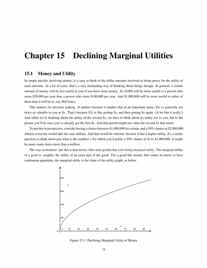
Chapter 15 Declining Marginal Utilities

15.1 Money and UtilityIn simple puzzles involving money, it is easy to think of the dollar amounts involved as being proxy for the utility of

each outcome. In a lot of cases, that’s a very misleading way of thinking about things though. In general, a certain

amount of money will be less useful to you if you have more money. So $1000 will be more useful to a person who

earns $20,000 per year than a person who earns $100,000 per year. And $1,000,000 will be more useful to either of

them than it will be to, say, Bill Gates.

This matters for decision making. It matters because it implies that in an important sense, $2x is generally not

twice as valuable to you as $x. That’s because $2x is like getting $x, and then getting $x again. (A lot like it really!)

And when we’re thinking about the utility of the second $x, we have to think about its utility not to you, but to the

person you’ll be once you’ve already got the first $x. And that person might not value the second $x that much.

To put this in perspective, consider having a choice between $1,000,000 for certain, and a 50% chance at $2,000,000.

Almost everyone would take the sure million. And that would be rational, because it has a higher utility. It’s a tricky

question to think about just what is the smallest x for which you’d prefer a 50% chance at $x to $1,000,000. It might

be many many times more than a million.

The way economists’ put this is that money (like most goods) has a declining marginal utility. The marginal utility

of a good is, roughly, the utility of an extra unit of the good. For a good like money that comes in (more or less)

continuous quantities, the marginal utility is the slope of the utility graph, as below.

0 10 20 30 40 50 60 70 80 90

80

160

240

320

Figure 15.1: Declining Marginal Utility of Money

73

15.2 Insurance 15. Declining Marginal Utilities

You should read the x-axis there are measuring possible incomes in thousands of dollars per year, and the y-axis as

measuring utility. The curve there is y = x12 . That isn’t necessarily a plausible account of how much utility each income

might give you, but it’s close enough for our purposes. Note that although more income gives you more utility, the

amount of extra utility you get from each extra bit of income goes down as you get more income. More precisely, the

slope of the income-utility graph keeps getting shallower and shallower as your income/utility rises. (More precisely

yet, a little calculus shows that the slope of the graph at any point is 12y , which is obviously always positive, but gets

less and less as your income/utility gets higher and higher.)

The fact that there is a declining marginal utility of money explains certain features of economic life. We’ll look at

models of two simple economic decisions, buying insurance and diversifying an investment portfolio. We’ll then use

what we said about diversified investments to explain some features of the actual insurance markets that we find.

15.2 InsuranceImagine the utility an agent gets from an income of x dollars is x

12 . And imagine that right now their income is $90,000.

But there is a 5% chance that something catastrophic will happen, and their income will be just $14,400. So their

expected income is 0.95×90,000+0.05×14,400 = 86220. But their expected utility is just 0.95×300+0.05×120 =

291, or the utility they would have with an income of $84,861.

Now imagine this person is offered insurance against the catastrophic scenario. They can pay, say, $4,736, and the

insurance company will restore the $75,600 that they will lose if the catastrophic event takes place. Their income is

now sure to be $85,264 (after the insurance is taken out), so they have a utility of 292. That’s higher than what their

utility was, so this is a good deal for them.

But note that it might also be a good deal for the insurance company. They receive in premiums $4,736. And

they have a 5% chance of paying out $75,600. So the expected outlay, in dollars, for them, is $3,780. So they turn an

expected profit on the deal. If they repeat this deal often enough, the probability that they will make a profit goes very

close to 1.

The point of the example is that people are trying to maximise expected utility, while insurance companies are

trying to maximise expected profits. Since there are cases where lowering your expected income can raise your

expected utility, there is a chance for a win-win trade. And this possibility, that expected income can go down while

expected utility can go up, is explained in virtue of the fact that there is a declining marginal utility of money.

15.3 DiversificationImagine that an agent has a starting wealth of 1, and the utility the agent gets from wealth x is x

12 . (We won’t specify

2 what, but take this to be some kind of substantial unit.) The agent has an opportunity to make an investment that has

a 50% chance of success and a 50% chance of failure. If the agent invests y in the scheme, the returns r will be

r =

4y, if success,

0, if failure.

The expected profit, in money, is y. That’s because there is a 50% chance of the profit being 3y, and a 50% chance of

it being −y. But in utility, the expected return of investing 1 unit is 0. The agent has a 50% chance of ending with a

wealth of 4, i.e. a utility of 2, and a 50% chance of ending with a wealth of 0, i.e. a utility of 0.

74

15. Declining Marginal Utilities 15.4 Selling Insurance

So making the investment doesn’t seem like a good idea. But now imagine that the agent could, instead of putting

all their money into this one venture, split the investment between two ventures that (a) have the same probability of

returns as this one, and (b) their success of failure is probabilistically independent. So the agent invests 12 in each deal.

The agent’s return will be

r =

4, if both succeed,

2, if one succeeds and the other fails,

0, if both fail.

The probability that both will succeed is 14 . The probability that one will succeed and the other fail is 1

2 . (Exercise:

why is this number greater?) The probability that both will fail is 14 . So the agent’s expected profit, in wealth, is 1.

That is, it is 4× 14 + 2× 1

2 + 0× 14 , i.e. 2, minus the 1 that is invested, so it is 2 minus 1, i.e. 1. So it’s the same as

before. Indeed, the expected profit on each investment is 12 . And the expected profits on a pair of investments is just

the sum of the expected profits on each of the investments.

But the expected utility of the ‘portfolio’ of two investments is considerably better than other portfolios with the

same expected profit. One such portfolio is investing all of the starting wealth in one 50/50 scheme. The expected

utility of the portfolio is 412 × 1

4 + 212 × 1

2 + 0× 14 , which is about 1.21. So it’s a much more valuable portfolio to the

agent than the portfolio which had just a single investment. Indeed, the diversified investment is worth making, while

the single investment was not worth making.

This is the general reason why it is good to have a diversified portfolio of investments. It isn’t because the expected

profits, measured in dollars, are higher this way. Indeed, diversification couldn’t possibly produce a higher expected

profit. That’s because the expected profit of a portfolio is just the sum of the expected profits of each investment in

the portfolio. What diversification can do is increase the expected utility of that return. Very roughly, the way it does

this is by decreasing the probability of the worst case scenarios, and of the best case scenarios. Because the worst case

scenario is more relevant to the expected utility calculation than the best case scenario, because in general it will be

further from the median outcome, the effect is to increase the expected utility overall.

One way of seeing how important diversification is is to consider what happens if the agent again makes two

investments like this, but the two investments are probabilistically linked. So if one investment succeeds, the other

has an 80% chance of success. Now the probability that both will succeed is 0.4, the probability that both will fail is

0.4, and the probability that one will succeed and the other fail is 0.2. The expected profit of the investments is still

1. (Each investment still has an expected profit of 12 , and expected profits are additive.) But the expected utility of

the portfolio is just 412 ×0.4+2

12 ×0.2+0×0.4, which is about 1.08. The return on investment, in utility terms, has

dropped by more than half.

The lesson is that for agents with declining marginal utilities for money, a diversified portfolio of investments can

be more valuable to them than any member of the portfolio on its own could be. But this fact turns on the investments

being probabilistically separated from one another.

15.4 Selling InsuranceIn the toy example about insurance, we assumed that the marginal utility of money for the insurance company was

flat. That isn’t really true. The insurance company is owned by people, and the utility of return to those people is

diminishing as the returns get higher. There is also the complication that the insurance company faces very different

75

15.4 Selling Insurance 15. Declining Marginal Utilities

kinds of returns when it is above and below the solvency line.

Nevertheless, the assumption that the marginal utility of money is constant for the insurance company is constant

is a useful fiction. And the reason that it is a useful fiction is that if the insurance company is well enough run, then

the assumption is close to being true. By ’well enough run’, I simply mean that their insurance portfolio is highly

diversified.

We won’t even try to prove this here, but there are various results in probability theory that suggest that as long

as there are a lot of different, and probabilistically independent, investments in a portfolio, then with a very high

probability, the actual returns will be close to the expected returns. In particular, if the expected returns are positive,

and the portfolio is large and diverse enough, then with a very high probability the actual returns will be positive. So,

at least in optimal cases, it isn’t a terrible simplification to treat the insurance company as if it was sure that it would

actually get its expected profits. And if that’s the case, the changing marginal utility of money is simply indifferent.

The mathematical results that are relevant here are what are sometimes called the ”Law of Large Numbers”. The

law says that if you sample independent and identically distributed random variables repeatedly, then for any positive

number e, the probability that the average output is within e of the expected output goes to 1 as the number of samples

goes to infinity. The approach can be quite quick in some cases. The following table lists the probability that the

number of heads on n flips of a random coin will be (strictly) between 0.4n and 0.6n for various values of n.

Number of flips Probabiilty of between 0.4n and 0.6n heads

1 0

10 0.246

20 0.497

50 0.797

100 0.943

200 0.994

500 > 0.99

This depends crucially on independence. If the coin flips were all perfectly dependent, then the probabilities would

not converge at all.

Note we’ve made two large assumptions about insurance companies. One is that the insurance company is large,

the other is that it is diversified. Arguably both of these assumptions are true of most real-world insurance companies.

There tend to be very few insurance companies in most economies. More importantly, those companies tend to be

fairly diversified. You can see this in a couple of different features of modern insurance companies.

One is that they work across multiple sectors. Most car insurance companies will also offer home insurance.

Compare this to other industries. It isn’t common for car sales agents to also be house sales agents. And it isn’t

common for car builders to also be house builders. The insurance industry tends to be special here. And that’s because

it’s very attractive for the insurance companies to have somewhat independent business wings, such as car insurance

and house insurance.

Another is that the products that are offered tend to be insurance on events that are somewhat probabilistically

independent. If I get in a car accident, this barely makes a difference to the probability that you’ll be in a car accident.

So offering car insurance is an attractive line of business. Other areas of life are a little trickier to insure. If I lose my

home to a hurricane, that does increase, perhaps substantially, the probability of you losing your house to a hurricane.

76

15. Declining Marginal Utilities 15.4 Selling Insurance

That’s because the probability of their being a hurricane, conditional on my losing my house to a hurricane, is 1. And

conditional on their being a hurricane, the probability of you losing your house to a hurricane rises substantially. So

offering hurricane insurance isn’t as attractive a line of business as car insurance. Finally, if I lose my home to an

invading army, the probability that the same will happen to you is very high indeed. In part for that reason, very few

companies ever offer ‘invasion insurance’.

It is very hard to say with certainty at this stage whether this is true, but it seems that a large part of the financial

crisis that is now ongoing is related to a similar problem. A lot of the financial institutions that failed were selling,

either explicitly or effectively, mortgage insurance. That is, they were insuring various banks against the possibility

of default. One problem with this is that mortgage defaults are not probabilistically independent. If I default on my

mortgage, that could be because I lost my job, or it could be because my house price collapsed and I have no interest

in sustaining my mortgage. Either way, the probability that you will also default goes up. (It goes up dramatically if

I defaulted for the second reason.) What may have been sensible insurance policies to write on their own turned into

massive losses because the insurers underestimated the probability of having to pay out on many policies all at once.

77

15.4 Selling Insurance 15. Declining Marginal Utilities

78

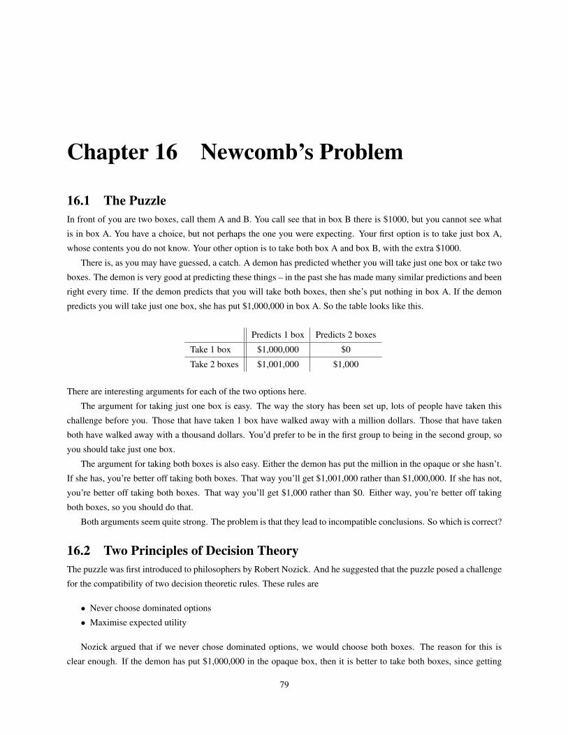
Chapter 16 Newcomb’s Problem

16.1 The PuzzleIn front of you are two boxes, call them A and B. You call see that in box B there is $1000, but you cannot see what

is in box A. You have a choice, but not perhaps the one you were expecting. Your first option is to take just box A,

whose contents you do not know. Your other option is to take both box A and box B, with the extra $1000.

There is, as you may have guessed, a catch. A demon has predicted whether you will take just one box or take two

boxes. The demon is very good at predicting these things – in the past she has made many similar predictions and been

right every time. If the demon predicts that you will take both boxes, then she’s put nothing in box A. If the demon

predicts you will take just one box, she has put $1,000,000 in box A. So the table looks like this.

Predicts 1 box Predicts 2 boxes

Take 1 box $1,000,000 $0

Take 2 boxes $1,001,000 $1,000

There are interesting arguments for each of the two options here.

The argument for taking just one box is easy. The way the story has been set up, lots of people have taken this

challenge before you. Those that have taken 1 box have walked away with a million dollars. Those that have taken

both have walked away with a thousand dollars. You’d prefer to be in the first group to being in the second group, so

you should take just one box.

The argument for taking both boxes is also easy. Either the demon has put the million in the opaque or she hasn’t.

If she has, you’re better off taking both boxes. That way you’ll get $1,001,000 rather than $1,000,000. If she has not,

you’re better off taking both boxes. That way you’ll get $1,000 rather than $0. Either way, you’re better off taking

both boxes, so you should do that.

Both arguments seem quite strong. The problem is that they lead to incompatible conclusions. So which is correct?

16.2 Two Principles of Decision TheoryThe puzzle was first introduced to philosophers by Robert Nozick. And he suggested that the puzzle posed a challenge

for the compatibility of two decision theoretic rules. These rules are

• Never choose dominated options

• Maximise expected utility

Nozick argued that if we never chose dominated options, we would choose both boxes. The reason for this is

clear enough. If the demon has put $1,000,000 in the opaque box, then it is better to take both boxes, since getting

79

16.3 Bringing Two Principles Together 16. Newcomb’s Problem

$1,001,000 is better than getting $1,000,000. And if the demon put nothing in the opaque box, then your choices are

$1,000 if you take both boxes, or $0 if you take just the empty box. Either way, you’re better off taking both boxes.

This is obviously just the standard argument for taking both boxes. But note that however plausible it is as an argument

for taking both boxes, it is compelling as an argument that taking both boxes is a dominating option.

To see why Nozick thought that maximising expected utility leads to taking one box, we need to see how he is

thinking of the expected utility formula. That formula takes as an input the probability of each state. Nozick’s way of

approaching things, which was the standard at the time, was to take the expected utility of an action A to be given by

the following sum

Exp(U(A)) = Pr(S1|A)U(AS1)+ ...+Pr(Sn|A)U(ASn)

Note in particular that we put into this formula the probability of each state given that A is chosen. We don’t take

the unconditional probability of being in that state. These numbers can come quite dramatically apart.

In Newcomb’s problem, it is actually quite hard to say what the probability of each state is. (The states here, of

course, are just that there is either $1,000,000 in the opaque box or that there is nothing in it.) But what’s easy to

say is the probability of each state given the choices you make. If you choose both boxes, the probability that there

is nothing in the opaque box is very high, and the probability that there is $1,000,000 in it is very low. Conversely, if

you choose just the one box, the probability that there is $1,000,000 in it is very high, and the probability that there is

nothing in it is very low. Simplifying just a little, we’ll say that this high probability is 1, and the low probabiilty is 0.

The expected utility of each choice then is

Exp(U(Take both boxes))

= Pr(Million in opaque box|Take both boxes)U(Take both boxes and million in opaque box)

+Pr(Nothing in opaque box|Take both boxes)U(Take both boxes and nothing in opaque box)

= 0×1,001,000+1×1,000

= 1,000

Exp(U(Take one box))

= Pr(Million in opaque box|Take one box)U(Take one box and million in opaque box)

+Pr(Nothing in opaque box|Take one box)U(Take one box and nothing in opaque box)

= 1×1,000,000+0×0

= 1,000,000

I’ve assumed here that the marginal utility of money is constant, so we can measure utility by the size of the

numerical prize. That’s an idealisation, but hopefully a harmless enough one.

16.3 Bringing Two Principles TogetherIn earlier chapters we argued that the expected utility rule never led to a conflict with the dominance principle. But

here it has led to a conflict. Something seems to have gone badly wrong.

80

16. Newcomb’s Problem 16.3 Bringing Two Principles Together

The problem was that we’ve used two distinct definitions of expected utility in the two arguments. In the version

we had used in previous chapters, we presupposed that the probability of the states was independent of the choices

that were made. So we didn’t talk about Pr(S1|A) or Pr(S1|B) or whatever. We simply talked about Pr(S1).

If you make that assumption, expected utility maximisation does indeed imply dominance. We won’t rerun the

entire proof here, but let’s see how it works in this particular case. Let’s say that the probability that there is $1,000,000

in the opaque box is x. It won’t matter at all what x is. And assume that the expected utility of a choice A is given by

this formula, where we use the unconditional probability of states as inputs.

Exp(U(A)) = Pr(S1)U(AS1)+ ...+Pr(Sn|A)U(ASn)

Applied to our particular case, that would give us the following calculations.

Exp(U(Take both boxes))

= Pr(Million in opaque box)U(Take both boxes and million in opaque box)

+Pr(Nothing in opaque box)U(Take both boxes and nothing in opaque box)

= x×1,001,000+(1− x)×1,000

= 1,000+1,000,000x

Exp(U(Take one box))

= Pr(Million in opaque box)U(Take one box and million in opaque box)

+Pr(Nothing in opaque box)U(Take one box and nothing in opaque box)

= x×1,000,000+(1− x)×0

= 1,000,000x

And clearly the expected value of taking both boxes is 1,000 higher than the expected utility of taking just one

box. So as long as we don’t conditionalise on the act we are performing, there isn’t a conflict between the dominance

principle and expected utility maximisation.

While that does resolve the mathematical puzzle, it hardly resolves the underlying philosophical problem. Why,

we might ask, shouldn’t we conditionalise on the actions we are performing? In general, it’s a bad idea to throw away

information, and the choice that we’re about to make is a piece of information. So we might think it should make a

difference to the probabilities that we are using.

The best response to this argument, I think, is that it leads to the wrong results in Newcomb’s problem, and related

problems. But this is a somewhat controversial clam. After all, some people think that taking one box is the right

result in Newcomb’s problem. And as we saw above, if we conditionalise on our action, then the expected utility

of taking one box is higher than the expected utility of taking both. So such theorists will not think that it gives the

wrong answer at all. To address this worry, we need to look more closely back at Newcomb’s original problem, and

its variants.

81

16.4 Well Meaning Friends 16. Newcomb’s Problem

16.4 Well Meaning FriendsThe next few sections are going to involve looking at arguments that we should take both boxes in Newcomb’s problem,

or to rejecting arguments that we should only take one box.

The simplest argument is just a dramatisation of the dominance argument. But still, it is a way to see the force of

that argument. Imagine that you have a friend who can see into the opaque box. Perhaps the box is clear from behind,

and your friend is standing behind the box. Or perhaps your friend has super-powers that let them see into opaque

boxes. If your friend was able to give you advice, and has your best interests at heart, they’ll tell you to take both

boxes. That’s true whether or not there is a million dollars in the opaque box. Either way, they’ll know that you’re

better off taking both boxes.

Of course, there are lots of cases where a friend with more knowledge than you and your interests at heart will

give you advice that is different to what you might intuitively think is correct. Imagine that I have just tossed a biased

coin that has an 80% chance of landing heads. The coin has landed, but neither of us can see how it has landed. I

offer you a choice between a bet that pays $1 if it landed heads, and a bet that pays $1 if it landed tails. Since heads is

more likely, it seems you should take the bet on heads. But if the coin has landed tails, then a well meaning and well

informed friend will tell you that you should bet on tails.

But that case is somewhat different to the friend in Newcomb’s problem. The point here is that you know what

the friend will tell you. And plausibly, whenever you know what advice a friend will give you, you should follow that

advice. Even in the coin-flip case, if you knew that your friend would tell you to bet on tails, it would be smart to

bet on tails. After all, knowing that your friend would give you that advice would be equivalent to knowing that the

coin landed tails. And if you knew the coin landed tails, then whatever arguments you could come up with concerning

chances of landing tails would be irrelevant. It did land tails, so that’s what you should bet on.

There is another way to dramatise the dominance argument. Imagine that after the boxes are opened, i.e. after you

know which state you are in, you are given a chance to revise your choice if you pay $500. If you take just one box,

then whatever is in the opaque box, this will be a worthwhile switch to make. It will either take you from $0 to $500,

or from $1,000,000 to $1,000,500. And once the box is open, there isn’t even an intuition that you should worry about

how the box got filled. So you should make the switch.

But it seems plausible in general that if right now you’ve got a chance to do X, and you know that if you don’t do

X now you’ll certainly pay good money to do X later, and you know that when you do that you’ll be acting perfectly

rationally, then you should simply do X. After all, you’ll get the same result whether you do X now or later, you’ll

simply not have to pay the ‘late fee’ for taking X any later. More relevantly to our case, if you would switch to X once

the facts were known, even if doing so required paying a fee, then it seems plausible that you should simply do X now.

It doesn’t seem that including the option of switching after the boxes are revealed changes anything about what you

should do before the boxes are revealed, after all.

Ultimately, I’m not sure that either of the arguments I gave here, either the well meaning friend argument or the

switching argument, are any more powerful than the dominance argument. Both of them are just ways of dramatising

the dominance argument. And someone who thinks that you should take just one box is, by definition, someone who

isn’t moved by the dominance argument. In the next set of notes we’ll look at other arguments for taking both boxes.

82

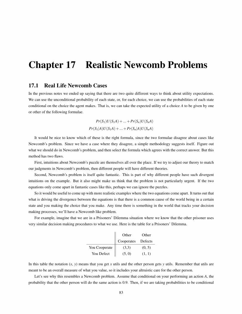
Chapter 17 Realistic Newcomb Problems

17.1 Real Life Newcomb CasesIn the previous notes we ended up saying that there are two quite different ways to think about utility expectations.

We can use the unconditional probability of each state, or, for each choice, we can use the probabilities of each state

conditional on the choice the agent makes. That is, we can take the expected utility of a choice A to be given by one

or other of the following formulae.

Pr(S1)U(S1A)+ ...+Pr(Sn)U(SnA)

Pr(S1|A)U(S1A)+ ...+Pr(Sn|A)U(SnA)

It would be nice to know which of these is the right formula, since the two formulae disagree about cases like

Newcomb’s problem. Since we have a case where they disagree, a simple methodology suggests itself. Figure out

what we should do in Newcomb’s problem, and then select the formula which agrees with the correct answer. But this

method has two flaws.

First, intuitions about Newcomb’s puzzle are themselves all over the place. If we try to adjust our theory to match

our judgments in Newcomb’s problem, then different people will have different theories.

Second, Newcomb’s problem is itself quite fantastic. This is part of why different people have such divergent

intuitions on the example. But it also might make us think that the problem is not particularly urgent. If the two

equations only come apart in fantastic cases like this, perhaps we can ignore the puzzles.

So it would be useful to come up with more realistic examples where the two equations come apart. It turns out that

what is driving the divergence between the equations is that there is a common cause of the world being in a certain

state and you making the choice that you make. Any time there is something in the world that tracks your decision

making processes, we’ll have a Newcomb like problem.

For example, imagine that we are in a Prisoners’ Dilemma situation where we know that the other prisoner uses

very similar decision making procedures to what we use. Here is the table for a Prisoners’ Dilemma.

Other Other

Cooperates Defects

You Cooperate (3,3) (0, 5)

You Defect (5, 0) (1, 1)

In this table the notation (x, y) means that you get x utils and the other person gets y utils. Remember that utils are

meant to be an overall measure of what you value, so it includes your altruistic care for the other person.

Let’s see why this resembles a Newcomb problem. Assume that conditional on your performing an action A, the

probability that the other person will do the same action is 0.9. Then, if we are taking probabilities to be conditional

83

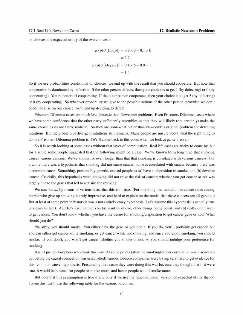
17.1 Real Life Newcomb Cases 17. Realistic Newcomb Problems

on choices, the expected utility of the two choices is

Exp(U(Coop)) = 0.9×3+0.1×0

= 2.7

Exp(U(De f ect)) = 0.1×5+0.9×1

= 1.4

So if we use probabilities conditional on choices, we end up with the result that you should cooperate. But note that

cooperation is dominated by defection. If the other person defects, then your choice is to get 1 (by defecting) or 0 (by

cooperating). You’re better off cooperating. If the other person cooperates, then your choice is to get 5 (by defecting)

or 0 (by cooperating). So whatever probability we give to the possible actions of the other person, provided we don’t

conditionalise on our choice, we’ll end up deciding to defect.

Prisoners Dilemma cases are much less fantastic than Newcomb problems. Even Prisoners Dilemma cases where

we have some confidence that the other party sufficiently resembles us that they will likely (not certainly) make the

same choice as us are fairly realistic. So they are somewhat better than Newcomb’s original problem for detecting

intuitions. But the problem of divergent intuitions still remains. Many people are unsure about what the right thing to

do in a Prisoners Dilemma problem is. (We’ll come back to this point when we look at game theory.)

So it is worth looking at some cases without that layer of complication. Real life cases are tricky to come by, but

for a while some people suggested that the following might be a case. We’ve known for a long time that smoking

causes various cancers. We’ve known for even longer than that that smoking is correlated with various cancers. For

a while there was a hypothesis that smoking did not cause cancer, but was correlated with cancer because there was

a common cause. Something, presumably genetic, caused people to (a) have a disposition to smoke, and (b) develop

cancer. Crucially, this hypothesis went, smoking did not raise the risk of cancer; whether you got cancer or not was

largely due to the genes that led to a desire for smoking.

We now know, by means of various tests, that this isn’t true. (For one thing, the reduction in cancer rates among

people who give up smoking is truly impressive, and hard to explain on the model that these cancers are all genetic.)

But at least at some point in history it was a not entirely crazy hypothesis. Let’s assume this hypothesis is actually true

(contrary to fact). And let’s assume that you (a) want to smoke, other things being equal, and (b) really don’t want

to get cancer. You don’t know whether you have the desire for smoking/disposition to get cancer gene or not? What

should you do?

Plausibly, you should smoke. You either have the gene or you don’t. If you do, you’ll probably get cancer, but

you can either get cancer while smoking, or get cancer while not smoking, and since you enjoy smoking, you should

smoke. If you don’t, you won’t get cancer whether you smoke or not, so you should indulge your preference for

smoking.

It isn’t just philosophers who think this way. At some points (after the smoking/cancer correlation was discovered

but before the causal connection was established) various tobacco companies were trying very hard to get evidence for

this ‘common cause’ hypothesis. Presumably the reason they were doing this was because they thought that if it were

true, it would be rational for people to smoke more, and hence people would smoke more.

But note that this presumption is true if and only if we use the ‘unconditional’ version of expected utility theory.

To see this, we’ll use the following table for the various outcomes.

84

17. Realistic Newcomb Problems 17.2 Tickle Defence

Get Cancer Don’t get Cancer

Smoke 1 6

Don’t Smoke 0 5

The assumption is that not getting cancer is worth 5 to you, while smoking is worth 1 to you. Now we know that

smoking is evidence that you have the cancer gene, and this raises dramatically the chance of you getting cancer.

So the (evidential) probability of getting cancer conditional on smoking is, we’ll assume, 0.8, while the (evidential)

probability of getting cancer conditional on not smoking is, we’ll assume, 0.2. And remember this isn’t because cancer

causes smoking in our example, but rather that there is a common cause of the two. Still, this is enough to make the

expected utilities work out as follows.

Exp(U(Smoke)) = 0.8×1+0.2×6

= 2

Exp(U(Don′tSmoke)) = 0.2×0+0.8×5

= 4

And the recommendation is not to smoke, even though smoking dominates. This seems very odd. As it is some-

times put, the recommendation here seems to be a matter of managing the ‘news’, not managing the outcome. What’s

bad about smoking is that if you smoke you get some evidence that something bad is going to happen to you. In

particular, you get evidence that you have this cancer gene, and that’s really bad news to get because dramatically

raises the probability of getting cancer. But not smoking doesn’t mean that you don’t have the gene, it just means that

you don’t find out that you have the gene. Not smoking looks like a policy of denying yourself good outcomes because

you don’t want to get bad news. And this doesn’t look rational.

So this case has convinced a lot of decision theorists that we shouldn’t use conditional probabilities of states when

working out the utility of various outcomes. Using conditional probabilities will be good if we want to learn the ‘news

value’ of some choices, but not if we want to learn how useful those choices will be to us.

17.2 Tickle DefenceNot everyone has been convinced by these ‘real-life’ examples. The counter-argument is that in any realistic case, the

gene that leads to smoking has to work by changing our dispositions. So there isn’t just a direct causal connection

between some genetic material and smoking. Rather, the gene causes a desire to smoke, and the desire to smoke cause

the smoking. As it is sometimes put, between the gene and the smoking there has to be something mental, a ‘tickle’

that leads to the smoking.

Now this is important because we might think that rational agents know their own mental states. Let’s assume that

for now. So if an agent has the smoking desire they know it, perhaps because this desire has a distinctive phenomenol-

ogy, a tickle of sorts. And if the agent knows this, then they won’t get any extra evidence that they have a desire to

smoke from their actual smoking. So the probability of getting cancer given smoking is not higher than the probability

of getting cancer given not smoking.

In the case we have in mind, the bad news is probably already here. Once the agent realises that their values

are given by the table above, they’ve already got the bad news. Someone who didn’t have the gene wouldn’t value

smoking more than not smoking. Once the person conditionalises on the fact that that is their value table, the evidence

85

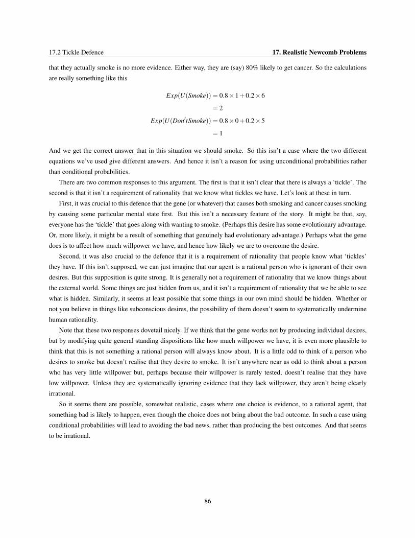
17.2 Tickle Defence 17. Realistic Newcomb Problems

that they actually smoke is no more evidence. Either way, they are (say) 80% likely to get cancer. So the calculations

are really something like this

Exp(U(Smoke)) = 0.8×1+0.2×6

= 2

Exp(U(Don′tSmoke)) = 0.8×0+0.2×5

= 1

And we get the correct answer that in this situation we should smoke. So this isn’t a case where the two different

equations we’ve used give different answers. And hence it isn’t a reason for using unconditional probabilities rather

than conditional probabilities.

There are two common responses to this argument. The first is that it isn’t clear that there is always a ‘tickle’. The

second is that it isn’t a requirement of rationality that we know what tickles we have. Let’s look at these in turn.

First, it was crucial to this defence that the gene (or whatever) that causes both smoking and cancer causes smoking

by causing some particular mental state first. But this isn’t a necessary feature of the story. It might be that, say,

everyone has the ‘tickle’ that goes along with wanting to smoke. (Perhaps this desire has some evolutionary advantage.

Or, more likely, it might be a result of something that genuinely had evolutionary advantage.) Perhaps what the gene

does is to affect how much willpower we have, and hence how likely we are to overcome the desire.

Second, it was also crucial to the defence that it is a requirement of rationality that people know what ‘tickles’

they have. If this isn’t supposed, we can just imagine that our agent is a rational person who is ignorant of their own

desires. But this supposition is quite strong. It is generally not a requirement of rationality that we know things about

the external world. Some things are just hidden from us, and it isn’t a requirement of rationality that we be able to see

what is hidden. Similarly, it seems at least possible that some things in our own mind should be hidden. Whether or

not you believe in things like subconscious desires, the possibility of them doesn’t seem to systematically undermine

human rationality.

Note that these two responses dovetail nicely. If we think that the gene works not by producing individual desires,

but by modifying quite general standing dispositions like how much willpower we have, it is even more plausible to

think that this is not something a rational person will always know about. It is a little odd to think of a person who

desires to smoke but doesn’t realise that they desire to smoke. It isn’t anywhere near as odd to think about a person

who has very little willpower but, perhaps because their willpower is rarely tested, doesn’t realise that they have

low willpower. Unless they are systematically ignoring evidence that they lack willpower, they aren’t being clearly

irrational.

So it seems there are possible, somewhat realistic, cases where one choice is evidence, to a rational agent, that

something bad is likely to happen, even though the choice does not bring about the bad outcome. In such a case using

conditional probabilities will lead to avoiding the bad news, rather than producing the best outcomes. And that seems

to be irrational.

86

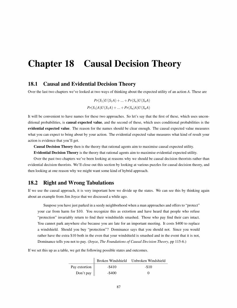
Chapter 18 Causal Decision Theory

18.1 Causal and Evidential Decision TheoryOver the last two chapters we’ve looked at two ways of thinking about the expected utility of an action A. These are

Pr(S1)U(S1A)+ ...+Pr(Sn)U(SnA)

Pr(S1|A)U(S1A)+ ...+Pr(Sn|A)U(SnA)

It will be convenient to have names for these two approaches. So let’s say that the first of these, which uses uncon-

ditional probabilities, is causal expected value, and the second of these, which uses conditional probabilities is the

evidential expected value. The reason for the names should be clear enough. The causal expected value measures

what you can expect to bring about by your action. The evidential expected value measures what kind of result your

action is evidence that you’ll get.

Causal Decision Theory then is the theory that rational agents aim to maximise causal expected utility.

Evidential Decision Theory is the theory that rational agents aim to maximise evidential expected utility.

Over the past two chapters we’ve been looking at reasons why we should be causal decision theorists rather than

evidential decision theorists. We’ll close out this section by looking at various puzzles for causal decision theory, and

then looking at one reason why we might want some kind of hybrid approach.

18.2 Right and Wrong TabulationsIf we use the causal approach, it is very important how we divide up the states. We can see this by thinking again

about an example from Jim Joyce that we discussed a while ago.

Suupose you have just parked in a seedy neighborhood when a man approaches and offers to “protect”

your car from harm for $10. You recognize this as extortion and have heard that people who refuse

“protection” invariably return to find their windshields smashed. Those who pay find their cars intact.

You cannot park anywhere else because you are late for an important meeting. It costs $400 to replace

a windshield. Should you buy “protection”? Dominance says that you should not. Since you would

rather have the extra $10 both in the even that your windshield is smashed and in the event that it is not,

Dominance tells you not to pay. (Joyce, The Foundations of Causal Decision Theory, pp 115-6.)

If we set this up as a table, we get the following possible states and outcomes.

Broken Windshield Unbroken Windshield

Pay extortion -$410 -$10

Don’t pay -$400 0

87

18.3 Why Ain’Cha Rich 18. Causal Decision Theory

Now if you look at the causal expected value of each action, the expected value of not paying will be higher. And this

will be so whatever probabilities you assign to broken windshield and unbroken windshield. Say that the probability

of the first is x and of the second is 1− x. Then we’ll have the following (assuming dollars equal utils)

Exp(U(Pay extortion)) =−410x−10(1− x)

=−400x−10

Exp(U(Don’t pay) =−400x−0(1− x)

=−400x

Whatever x is, the causal expected value of not paying is higher by 10. That’s obviously a bad result. Is it a

problem for causal decision theory though? No. As the name ‘causal’ suggests, it is crucial to causal decision theory

that we separate out what we have causal power over from what we don’t have causal power over. The states of the

world represent what we can’t control. If something can be causally affected by our actions, it can’t be a background

state.

So this is a complication in applying causal decision theory. Note that it is not a problem for evidential decision

theory. We can even use the very table that we have there. Let’s assume that the probability of broken windshield

given paying is 0, and the probability of unbroken windshield given paying is 0. Then the expected utilities will work

out as follows

Exp(U(Pay extortion)) =−410×0−10×1

=−10

Exp(U(Don’t pay) =−400×1−10×0

=−400

So we get the right result that we should pay up. It is a nice feature of evidential decision theory that we don’t have

to be so careful about what states are and aren’t under our control. Of course, if the only reason we don’t have to

worry about what is and isn’t under our control is that the theory systematically ignores such facts, even though they

are intuitively relevant to decision theory, this isn’t perhaps the best advertisement for evidential decision theory.

18.3 Why Ain’Cha RichThere is one other argument for evidential decision theory that we haven’t yet addressed. Causal decision theory

recommends taking two boxes in Newcomb’s problem; evidential decision theory recommends only taking one. People

who take both boxes tend, as a rule, to end up poorer than people who take just the one box. Since the aim here is to

get the best outcome, this might be thought to be embarrassing for causal decision theorists.

Causal decision theorists have a response to this argument. They say that Newcomb’s problem is a situation where

there is someone who is quite smart, and quite determined to reward irrationality. In such a case, they say, it isn’t too

surprising that irrational people, i.e. evidential decision theorists, get rewarded. Moreover, if a rational person like

them were to have taken just one box, they would have ended up with even less money, i.e., they would have ended up

with nothing.

One way that causal decision theorists would have liked to make this objection stronger would be to show that

there is a universal problem for decision theories - whenever there is someone whose aim is to reward people who

88

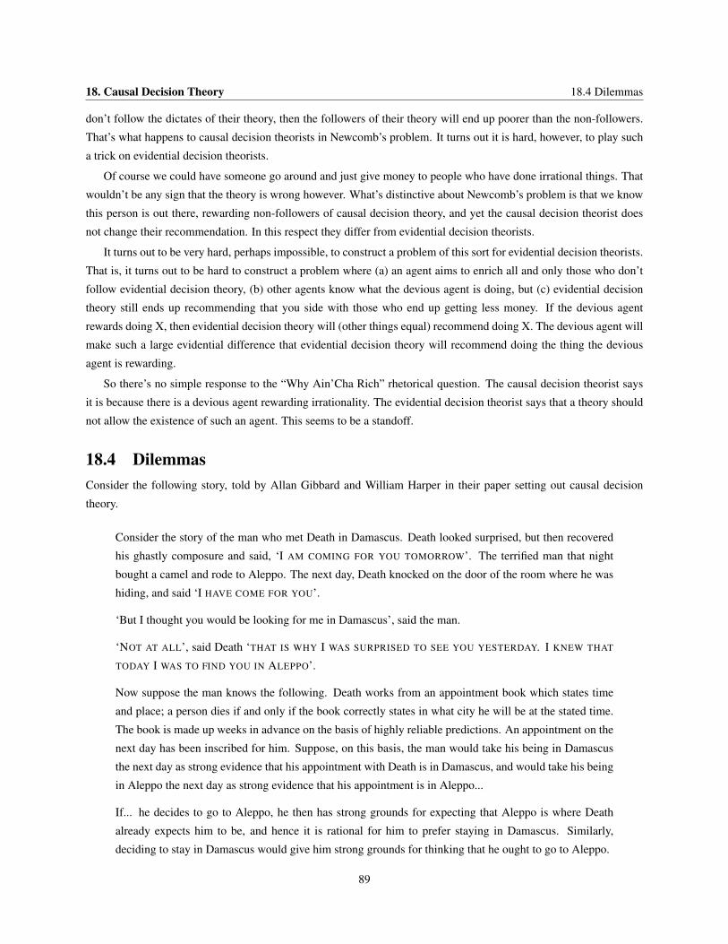
18. Causal Decision Theory 18.4 Dilemmas

don’t follow the dictates of their theory, then the followers of their theory will end up poorer than the non-followers.

That’s what happens to causal decision theorists in Newcomb’s problem. It turns out it is hard, however, to play such

a trick on evidential decision theorists.

Of course we could have someone go around and just give money to people who have done irrational things. That

wouldn’t be any sign that the theory is wrong however. What’s distinctive about Newcomb’s problem is that we know

this person is out there, rewarding non-followers of causal decision theory, and yet the causal decision theorist does

not change their recommendation. In this respect they differ from evidential decision theorists.

It turns out to be very hard, perhaps impossible, to construct a problem of this sort for evidential decision theorists.

That is, it turns out to be hard to construct a problem where (a) an agent aims to enrich all and only those who don’t

follow evidential decision theory, (b) other agents know what the devious agent is doing, but (c) evidential decision

theory still ends up recommending that you side with those who end up getting less money. If the devious agent

rewards doing X, then evidential decision theory will (other things equal) recommend doing X. The devious agent will

make such a large evidential difference that evidential decision theory will recommend doing the thing the devious

agent is rewarding.

So there’s no simple response to the “Why Ain’Cha Rich” rhetorical question. The causal decision theorist says

it is because there is a devious agent rewarding irrationality. The evidential decision theorist says that a theory should

not allow the existence of such an agent. This seems to be a standoff.

18.4 DilemmasConsider the following story, told by Allan Gibbard and William Harper in their paper setting out causal decision

theory.

Consider the story of the man who met Death in Damascus. Death looked surprised, but then recovered

his ghastly composure and said, ‘I AM COMING FOR YOU TOMORROW’. The terrified man that night

bought a camel and rode to Aleppo. The next day, Death knocked on the door of the room where he was

hiding, and said ‘I HAVE COME FOR YOU’.

‘But I thought you would be looking for me in Damascus’, said the man.

‘NOT AT ALL’, said Death ‘THAT IS WHY I WAS SURPRISED TO SEE YOU YESTERDAY. I KNEW THAT

TODAY I WAS TO FIND YOU IN ALEPPO’.

Now suppose the man knows the following. Death works from an appointment book which states time

and place; a person dies if and only if the book correctly states in what city he will be at the stated time.

The book is made up weeks in advance on the basis of highly reliable predictions. An appointment on the

next day has been inscribed for him. Suppose, on this basis, the man would take his being in Damascus

the next day as strong evidence that his appointment with Death is in Damascus, and would take his being

in Aleppo the next day as strong evidence that his appointment is in Aleppo...

If... he decides to go to Aleppo, he then has strong grounds for expecting that Aleppo is where Death

already expects him to be, and hence it is rational for him to prefer staying in Damascus. Similarly,

deciding to stay in Damascus would give him strong grounds for thinking that he ought to go to Aleppo.

89

18.5 Weak Newcomb Problems 18. Causal Decision Theory

In cases like this, the agent is in a real dilemma. Whatever he does, it seems that it will be the wrong thing. If he goes

to Aleppo, then Death will probably be there. And if he stays in Damascus, then Death will probably be there as well.

So it seems like he is stuck.

Of course in one sense, there is clearly a right thing to do, namely go wherever Death isn’t. But that isn’t the sense

of right decision we’re typically using in decision theory. Is there something that he can do that maximises expected

utility. In a sense the answer is “No”. Whatever he does, doing that will be some evidence that Death is elsewhere.

And what he should do is go wherever his evidence suggests Death isn’t. This turns out to be impossible, so the agent

is bound not to do the rational thing.

Is this a problem for causal decision theory? It is if you think that we should always have a rational option available

to us. If you think that ‘rational’ here is a kind of ‘ought’, and you think ‘ought’ implies ‘can’, then you might think

we have a problem, because in this case there’s a sense in which the man can’t do the right thing. (Though this is a bit

unclear; in the actual story, there’s a perfectly good sense in which he could have stayed in Aleppo, and the right thing

to do, given his evidence, would have been to stay in Aleppo. So in one sense he could have done the right thing.) But

both the premises of the little argument here are somewhat contentious. It isn’t clear that we should say you ought, in

any sense, maximise expected utility. And the principle that ought implies can is rather controversial. So perhaps this

isn’t a clear counterexample to causal decision theory.

18.5 Weak Newcomb ProblemsImagine a small change to the original Newcomb problem. Instead of there being $1000 in the clear box, there is

$800,000. Still, evidential decision theory recommends taking one box. The evidential expected value of taking both

boxes is now roughly $800,000, while the evidential expected value of taking just the one box is $1,000,000. Causal

decision theory recommends taking both boxes, as before.

So neither theory changes its recommendations when we increase the amount in the clear box. But I think many

people find the case for taking just the one box to be less compelling in this variant. Does that suggest we need a third

theory, other than just causal or evidential decision theory?

It turns out that we can come up with hybrid theories that recommend taking one box in the original case, but two

boxes in the original case. Remember that in principle anything can have a probability, including theories of decision.

So let’s pretend that given the (philosophical) evidence on the table, the probability of causal decision theory is, say,

0.8, while the probability of evidential decision theory is 0.2. (I’m not saying these numbers are right, this is just a

possibility to float.) And let’s say that we should do the thing that has the highest expected expected utility, where

we work out expected expected utilities by summing over the expectation of the action on different theories, times the

probability of each theory. (Again, I’m not endorsing this, just floating it.)

Now in the original Newcomb problem, evidential decision theory says taking one boxes is $999,000 better, while

causal decision theory say staking both boxes is $1,000 better. So the expected expected utility of taking one box

rather than both boxes is 0.2×999,000−0.8×1,000, which is 199,000. So taking one box is ‘better’ by 199,000

In the modified Newcomb problem, evidential decision theory says taking one boxes is $200,000 better, while

causal decision theory says taking both boxes is $800,000 better. So the expected expected utility of taking one box

rather than both boxes is 0.2×200,000−0.8×800,000, i.e., -600,000. So taking both boxes is ‘better’ by 600,000.

If you think that changing the amount in the clear box can change your decision in Newcomb’s problem, then

possibly you want a hybrid theory, perhaps like the one floated here.

90

Chapter 19 Introduction to Games

19.1 GamesA game is any decision problem where the outcome turns on the actions of two or more individuals. We’ll entirely be

concerned here with games where the outcome turns on the actions of just two agents, though that’s largely because

the larger cases are more mathematically complicated.

Given a definition that broad, pretty much any human interaction can be described as a game. And indeed game

theory, the study of games in this sense, is one of the most thriving areas of modern decision theory. Game theory is

routinely used in thinking about conflicts, such as warfare or elections. It is also used in thinking about all sorts of

economic interactions. Game theorists have played crucial (and lucrative) roles in recent years designing high-profile

auctions, for example. The philosopher and economist Ken Binmore, for example, led the team that used insights from

modern game theory to design the auction of the 3G wireless spectrum in Britain. That auction yielded the government

billions of pounds more than was anticipated.

When we think of the ordinary term ‘game’, we naturally think of games like football or chess, where there are

two players with conflicting goals. But these games are really quite special cases. What’s distinctive of football and

chess is that, to a first approximation, the players’ goals are completely in conflict. Whatever is good for the interests

of one player is bad for the interests of the other player. This isn’t what’s true of most human interaction. Most human

interaction is not, as we will put it here, zero sum. When we say that an interaction is zero sum, what we mean

(roughly) that the net outcome for the players is constant. (Such games may better be called ‘constant-sum’.)

We’ll generally represent games using tables like the following. Each row represents a possible move (or strategy)

for a player called Row, and each column represents a possible move (or strategy) for a player called Column. Each

cell represents the payoffs for the two players. The first number is the utility that Row receives for that outcome, and

the second number is the utility that Column receives for that outcome. Here is an example of a game. (It’s a version

of a game called the Stag Hunt.)

Team Solo

Team (4, 4) (1, 3)

Solo (3, 1) (3, 3)

Each player has a choice between two strategies, one called ‘Team’ and the other called ‘Solo’. (The model here is

whether players choose to hunt alone or as a team. A team produces better results for everyone; if it is large enough.)

Whoever plays Solo is guaranteed to get an outcome of 3. If someone plays Team, they get 4 if the other player plays

Team as well, and 1 if the other player plays solo.

A zero sum game is where the outcomes all sum to a constant. (For simplicity, we usually make this constant zero.)

So here is a representation of (a single game of) Rock-Paper-Scissors.

91

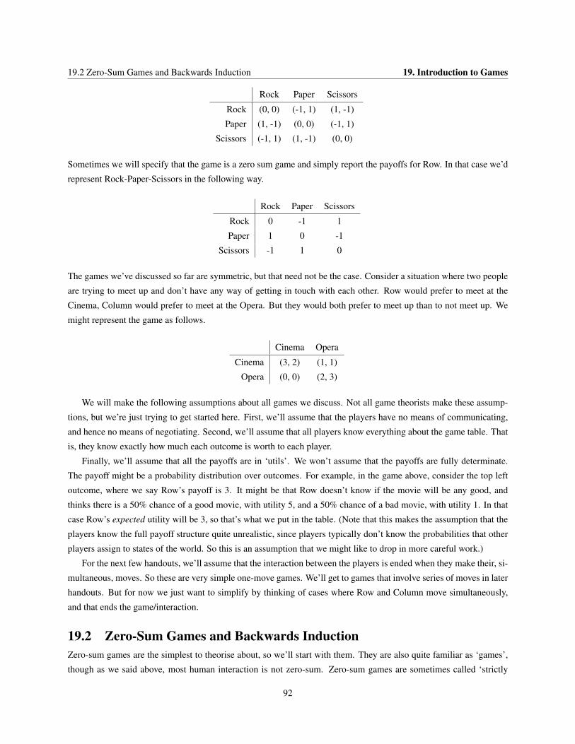
19.2 Zero-Sum Games and Backwards Induction 19. Introduction to Games

Rock Paper Scissors

Rock (0, 0) (-1, 1) (1, -1)

Paper (1, -1) (0, 0) (-1, 1)

Scissors (-1, 1) (1, -1) (0, 0)

Sometimes we will specify that the game is a zero sum game and simply report the payoffs for Row. In that case we’d

represent Rock-Paper-Scissors in the following way.

Rock Paper Scissors

Rock 0 -1 1

Paper 1 0 -1

Scissors -1 1 0

The games we’ve discussed so far are symmetric, but that need not be the case. Consider a situation where two people

are trying to meet up and don’t have any way of getting in touch with each other. Row would prefer to meet at the

Cinema, Column would prefer to meet at the Opera. But they would both prefer to meet up than to not meet up. We

might represent the game as follows.

Cinema Opera

Cinema (3, 2) (1, 1)

Opera (0, 0) (2, 3)

We will make the following assumptions about all games we discuss. Not all game theorists make these assump-

tions, but we’re just trying to get started here. First, we’ll assume that the players have no means of communicating,

and hence no means of negotiating. Second, we’ll assume that all players know everything about the game table. That

is, they know exactly how much each outcome is worth to each player.

Finally, we’ll assume that all the payoffs are in ‘utils’. We won’t assume that the payoffs are fully determinate.

The payoff might be a probability distribution over outcomes. For example, in the game above, consider the top left

outcome, where we say Row’s payoff is 3. It might be that Row doesn’t know if the movie will be any good, and

thinks there is a 50% chance of a good movie, with utility 5, and a 50% chance of a bad movie, with utility 1. In that

case Row’s expected utility will be 3, so that’s what we put in the table. (Note that this makes the assumption that the

players know the full payoff structure quite unrealistic, since players typically don’t know the probabilities that other

players assign to states of the world. So this is an assumption that we might like to drop in more careful work.)

For the next few handouts, we’ll assume that the interaction between the players is ended when they make their, si-

multaneous, moves. So these are very simple one-move games. We’ll get to games that involve series of moves in later

handouts. But for now we just want to simplify by thinking of cases where Row and Column move simultaneously,

and that ends the game/interaction.

19.2 Zero-Sum Games and Backwards InductionZero-sum games are the simplest to theorise about, so we’ll start with them. They are also quite familiar as ‘games’,

though as we said above, most human interaction is not zero-sum. Zero-sum games are sometimes called ‘strictly

92

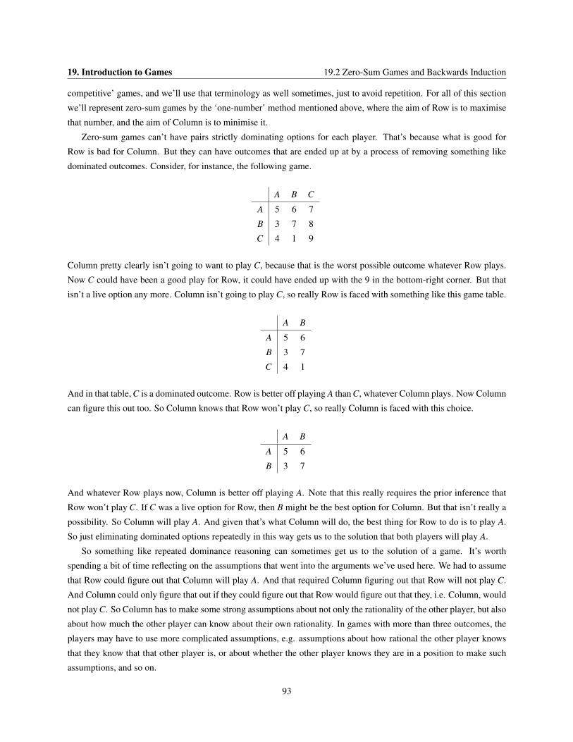
19. Introduction to Games 19.2 Zero-Sum Games and Backwards Induction

competitive’ games, and we’ll use that terminology as well sometimes, just to avoid repetition. For all of this section

we’ll represent zero-sum games by the ‘one-number’ method mentioned above, where the aim of Row is to maximise

that number, and the aim of Column is to minimise it.

Zero-sum games can’t have pairs strictly dominating options for each player. That’s because what is good for

Row is bad for Column. But they can have outcomes that are ended up at by a process of removing something like

dominated outcomes. Consider, for instance, the following game.

A B C

A 5 6 7

B 3 7 8

C 4 1 9

Column pretty clearly isn’t going to want to play C, because that is the worst possible outcome whatever Row plays.

Now C could have been a good play for Row, it could have ended up with the 9 in the bottom-right corner. But that

isn’t a live option any more. Column isn’t going to play C, so really Row is faced with something like this game table.

A B

A 5 6

B 3 7

C 4 1

And in that table, C is a dominated outcome. Row is better off playing A than C, whatever Column plays. Now Column

can figure this out too. So Column knows that Row won’t play C, so really Column is faced with this choice.

A B

A 5 6

B 3 7

And whatever Row plays now, Column is better off playing A. Note that this really requires the prior inference that

Row won’t play C. If C was a live option for Row, then B might be the best option for Column. But that isn’t really a

possibility. So Column will play A. And given that’s what Column will do, the best thing for Row to do is to play A.

So just eliminating dominated options repeatedly in this way gets us to the solution that both players will play A.

So something like repeated dominance reasoning can sometimes get us to the solution of a game. It’s worth

spending a bit of time reflecting on the assumptions that went into the arguments we’ve used here. We had to assume

that Row could figure out that Column will play A. And that required Column figuring out that Row will not play C.

And Column could only figure that out if they could figure out that Row would figure out that they, i.e. Column, would

not play C. So Column has to make some strong assumptions about not only the rationality of the other player, but also

about how much the other player can know about their own rationality. In games with more than three outcomes, the

players may have to use more complicated assumptions, e.g. assumptions about how rational the other player knows

that they know that that other player is, or about whether the other player knows they are in a position to make such

assumptions, and so on.

93

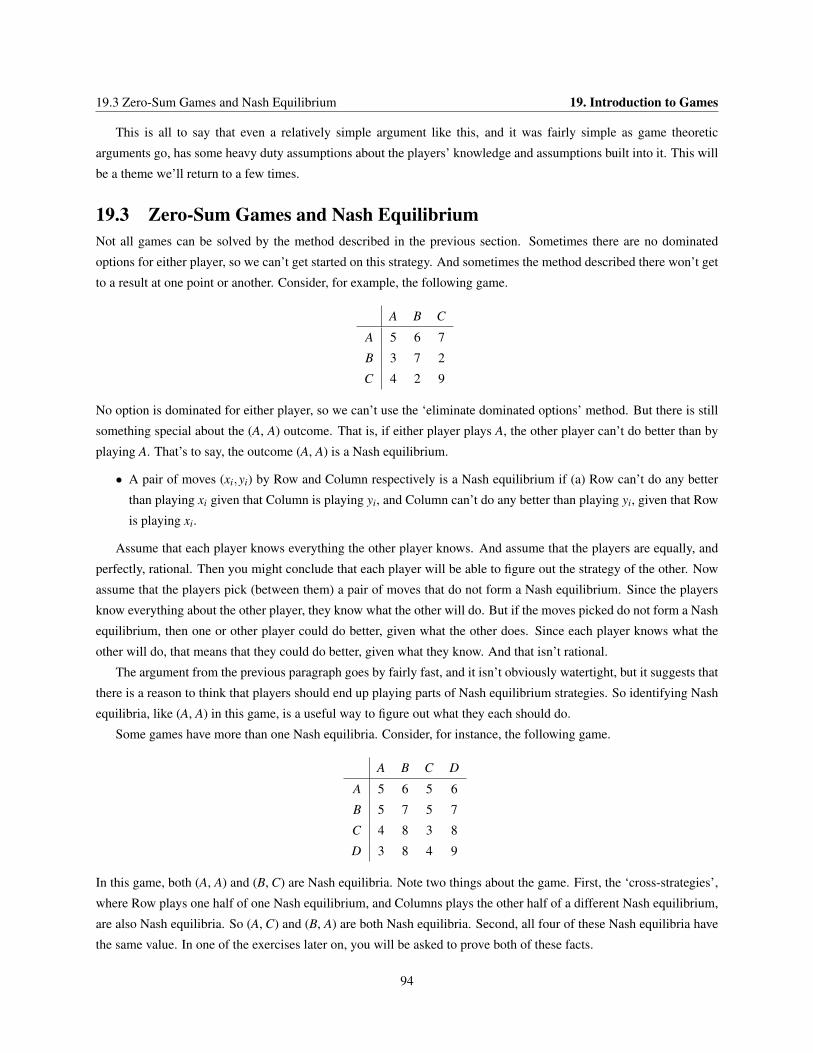
19.3 Zero-Sum Games and Nash Equilibrium 19. Introduction to Games

This is all to say that even a relatively simple argument like this, and it was fairly simple as game theoretic

arguments go, has some heavy duty assumptions about the players’ knowledge and assumptions built into it. This will

be a theme we’ll return to a few times.

19.3 Zero-Sum Games and Nash EquilibriumNot all games can be solved by the method described in the previous section. Sometimes there are no dominated

options for either player, so we can’t get started on this strategy. And sometimes the method described there won’t get

to a result at one point or another. Consider, for example, the following game.

A B C

A 5 6 7

B 3 7 2

C 4 2 9

No option is dominated for either player, so we can’t use the ‘eliminate dominated options’ method. But there is still

something special about the (A, A) outcome. That is, if either player plays A, the other player can’t do better than by

playing A. That’s to say, the outcome (A, A) is a Nash equilibrium.

• A pair of moves (xi,yi) by Row and Column respectively is a Nash equilibrium if (a) Row can’t do any better

than playing xi given that Column is playing yi, and Column can’t do any better than playing yi, given that Row

is playing xi.

Assume that each player knows everything the other player knows. And assume that the players are equally, and

perfectly, rational. Then you might conclude that each player will be able to figure out the strategy of the other. Now

assume that the players pick (between them) a pair of moves that do not form a Nash equilibrium. Since the players

know everything about the other player, they know what the other will do. But if the moves picked do not form a Nash

equilibrium, then one or other player could do better, given what the other does. Since each player knows what the

other will do, that means that they could do better, given what they know. And that isn’t rational.

The argument from the previous paragraph goes by fairly fast, and it isn’t obviously watertight, but it suggests that

there is a reason to think that players should end up playing parts of Nash equilibrium strategies. So identifying Nash

equilibria, like (A, A) in this game, is a useful way to figure out what they each should do.

Some games have more than one Nash equilibria. Consider, for instance, the following game.

A B C D

A 5 6 5 6

B 5 7 5 7

C 4 8 3 8

D 3 8 4 9

In this game, both (A, A) and (B, C) are Nash equilibria. Note two things about the game. First, the ‘cross-strategies’,

where Row plays one half of one Nash equilibrium, and Columns plays the other half of a different Nash equilibrium,

are also Nash equilibria. So (A, C) and (B, A) are both Nash equilibria. Second, all four of these Nash equilibria have

the same value. In one of the exercises later on, you will be asked to prove both of these facts.

94

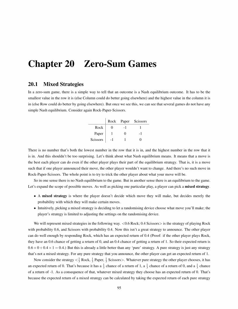
Chapter 20 Zero-Sum Games

20.1 Mixed StrategiesIn a zero-sum game, there is a simple way to tell that an outcome is a Nash equilibrium outcome. It has to be the

smallest value in the row it is (else Column could do better going elsewhere) and the highest value in the column it is

in (else Row could do better by going elsewhere). But once we see this, we can see that several games do not have any

simple Nash equilibrium. Consider again Rock-Paper-Scissors.

Rock Paper Scissors

Rock 0 -1 1

Paper 1 0 -1

Scissors -1 1 0

There is no number that’s both the lowest number in the row that it is in, and the highest number in the row that it

is in. And this shouldn’t be too surprising. Let’s think about what Nash equilibrium means. It means that a move is

the best each player can do even if the other player plays their part of the equilibrium strategy. That is, it is a move

such that if one player announced their move, the other player wouldn’t want to change. And there’s no such move in

Rock-Paper-Scissors. The whole point is to try to trick the other player about what your move will be.

So in one sense there is no Nash equilibrium to the game. But in another sense there is an equilibrium to the game.

Let’s expand the scope of possible moves. As well as picking one particular play, a player can pick a mixed strategy.

• A mixed strategy is where the player doesn’t decide which move they will make, but decides merely the

probability with which they will make certain moves.

• Intuitively, picking a mixed strategy is deciding to let a randomising device choose what move you’ll make; the

player’s strategy is limited to adjusting the settings on the randomising device.

We will represent mixed strategies in the following way. <0.6 Rock; 0.4 Scissors> is the strategy of playing Rock

with probability 0.6, and Scissors with probability 0.4. Now this isn’t a great strategy to announce. The other player

can do well enough by responding Rock, which has an expected return of 0.4 (Proof: if the other player plays Rock,

they have an 0.6 chance of getting a return of 0, and an 0.4 chance of getting a return of 1. So their expected return is

0.6×0+0.4×1 = 0.4.) But this is already a little better than any ‘pure’ strategy. A pure strategy is just any strategy

that’s not a mixed strategy. For any pure strategy that you announce, the other player can get an expected return of 1.

Now consider the strategy < 13 Rock, 1

3 Paper, 13 Scissors>. Whatever pure strategy the other player chooses, it has

an expected return of 0. That’s because it has a 13 chance of a return of 1, a 1

3 chance of a return of 0, and a 13 chance

of a return of -1. As a consequence of that, whatever mixed strategy they choose has an expected return of 0. That’s

because the expected return of a mixed strategy can be calculated by taking the expected return of each pure strategy

95

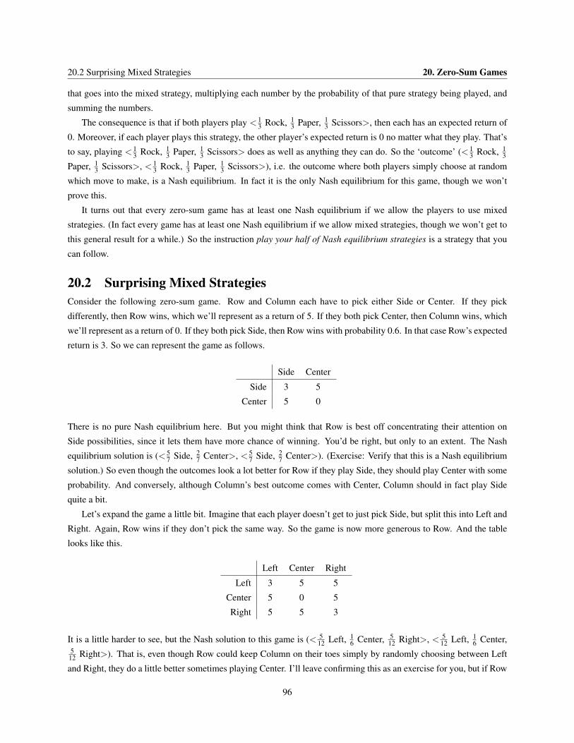
20.2 Surprising Mixed Strategies 20. Zero-Sum Games

that goes into the mixed strategy, multiplying each number by the probability of that pure strategy being played, and

summing the numbers.

The consequence is that if both players play < 13 Rock, 1

3 Paper, 13 Scissors>, then each has an expected return of

0. Moreover, if each player plays this strategy, the other player’s expected return is 0 no matter what they play. That’s

to say, playing < 13 Rock, 1

3 Paper, 13 Scissors> does as well as anything they can do. So the ‘outcome’ (< 1

3 Rock, 13

Paper, 13 Scissors>, < 1

3 Rock, 13 Paper, 1

3 Scissors>), i.e. the outcome where both players simply choose at random

which move to make, is a Nash equilibrium. In fact it is the only Nash equilibrium for this game, though we won’t

prove this.

It turns out that every zero-sum game has at least one Nash equilibrium if we allow the players to use mixed

strategies. (In fact every game has at least one Nash equilibrium if we allow mixed strategies, though we won’t get to

this general result for a while.) So the instruction play your half of Nash equilibrium strategies is a strategy that you

can follow.

20.2 Surprising Mixed StrategiesConsider the following zero-sum game. Row and Column each have to pick either Side or Center. If they pick

differently, then Row wins, which we’ll represent as a return of 5. If they both pick Center, then Column wins, which

we’ll represent as a return of 0. If they both pick Side, then Row wins with probability 0.6. In that case Row’s expected

return is 3. So we can represent the game as follows.

Side Center

Side 3 5

Center 5 0

There is no pure Nash equilibrium here. But you might think that Row is best off concentrating their attention on

Side possibilities, since it lets them have more chance of winning. You’d be right, but only to an extent. The Nash

equilibrium solution is (< 57 Side, 2

7 Center>, < 57 Side, 2

7 Center>). (Exercise: Verify that this is a Nash equilibrium

solution.) So even though the outcomes look a lot better for Row if they play Side, they should play Center with some

probability. And conversely, although Column’s best outcome comes with Center, Column should in fact play Side

quite a bit.

Let’s expand the game a little bit. Imagine that each player doesn’t get to just pick Side, but split this into Left and

Right. Again, Row wins if they don’t pick the same way. So the game is now more generous to Row. And the table

looks like this.

Left Center Right

Left 3 5 5

Center 5 0 5

Right 5 5 3

It is a little harder to see, but the Nash solution to this game is (< 512 Left, 1

6 Center, 512 Right>, < 5

12 Left, 16 Center,

512 Right>). That is, even though Row could keep Column on their toes simply by randomly choosing between Left

and Right, they do a little better sometimes playing Center. I’ll leave confirming this as an exercise for you, but if Row

96

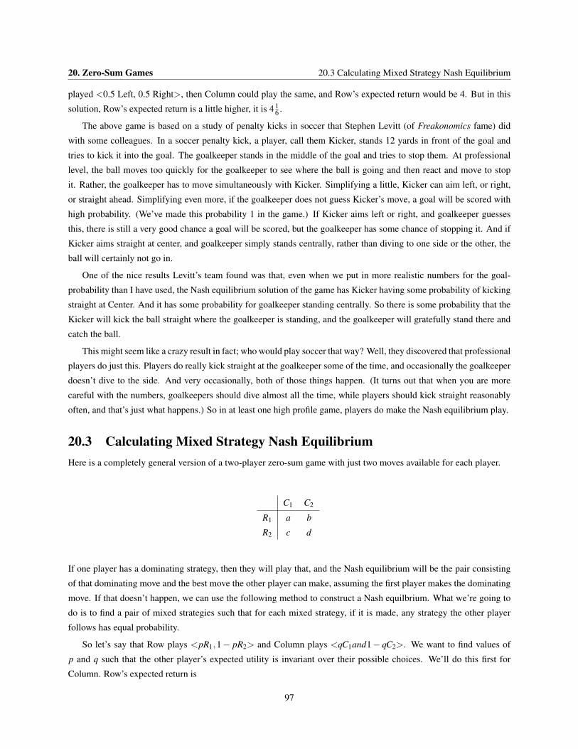
20. Zero-Sum Games 20.3 Calculating Mixed Strategy Nash Equilibrium

played <0.5 Left, 0.5 Right>, then Column could play the same, and Row’s expected return would be 4. But in this

solution, Row’s expected return is a little higher, it is 4 16 .

The above game is based on a study of penalty kicks in soccer that Stephen Levitt (of Freakonomics fame) did

with some colleagues. In a soccer penalty kick, a player, call them Kicker, stands 12 yards in front of the goal and

tries to kick it into the goal. The goalkeeper stands in the middle of the goal and tries to stop them. At professional

level, the ball moves too quickly for the goalkeeper to see where the ball is going and then react and move to stop

it. Rather, the goalkeeper has to move simultaneously with Kicker. Simplifying a little, Kicker can aim left, or right,

or straight ahead. Simplifying even more, if the goalkeeper does not guess Kicker’s move, a goal will be scored with

high probability. (We’ve made this probability 1 in the game.) If Kicker aims left or right, and goalkeeper guesses

this, there is still a very good chance a goal will be scored, but the goalkeeper has some chance of stopping it. And if

Kicker aims straight at center, and goalkeeper simply stands centrally, rather than diving to one side or the other, the

ball will certainly not go in.

One of the nice results Levitt’s team found was that, even when we put in more realistic numbers for the goal-

probability than I have used, the Nash equilibrium solution of the game has Kicker having some probability of kicking

straight at Center. And it has some probability for goalkeeper standing centrally. So there is some probability that the

Kicker will kick the ball straight where the goalkeeper is standing, and the goalkeeper will gratefully stand there and

catch the ball.

This might seem like a crazy result in fact; who would play soccer that way? Well, they discovered that professional

players do just this. Players do really kick straight at the goalkeeper some of the time, and occasionally the goalkeeper

doesn’t dive to the side. And very occasionally, both of those things happen. (It turns out that when you are more

careful with the numbers, goalkeepers should dive almost all the time, while players should kick straight reasonably

often, and that’s just what happens.) So in at least one high profile game, players do make the Nash equilibrium play.

20.3 Calculating Mixed Strategy Nash EquilibriumHere is a completely general version of a two-player zero-sum game with just two moves available for each player.

C1 C2

R1 a b

R2 c d

If one player has a dominating strategy, then they will play that, and the Nash equilibrium will be the pair consisting

of that dominating move and the best move the other player can make, assuming the first player makes the dominating

move. If that doesn’t happen, we can use the following method to construct a Nash equilbrium. What we’re going to

do is to find a pair of mixed strategies such that for each mixed strategy, if it is made, any strategy the other player

follows has equal probability.

So let’s say that Row plays <pR1,1− pR2> and Column plays <qC1and1− qC2>. We want to find values of

p and q such that the other player’s expected utility is invariant over their possible choices. We’ll do this first for

Column. Row’s expected return is

97

20.3 Calculating Mixed Strategy Nash Equilibrium 20. Zero-Sum Games

Pr(R1C1)U(R1C1)+Pr(R1C2)U(R1C2)+Pr(R2C1)U(R2C1)+Pr(R2C2)U(R2C2)

=pq×a+ p(1−q)×b+(1− p)q× c+(1− p)(1−q)×d

=pqa+ pb− pqb+qc− pqc+d− pd−qd + pqd

=p(qa+b−qb−qc−d +qd)+qc+d−qd

Now our aim is to make that value a constant when p varies. So we have to make qa+b−qb−qc−d +qd equal

0, and then Row’s expected return will be exactly qc+d−qd. So we have the following series of equations.

qa+b−qb−qc−d +qd = 0

qa+qd−qb−qc = d−b

q(a+d− (b+ c)) = d−b

q =d−b

a+d− (b+ c)

Let’s do the same thing for Row. Again, we’re assuming that there is no pure Nash equilibrium, and we’re trying

to find a mixed equilibrium. And in such a state, whatever Column does, it won’t change her expected return. Now

Column’s expected return is the negation of Row’s return. So her return is

Pr(R1C1)U(R1C1)+Pr(R1C2)U(R1C2)+Pr(R2C1)U(R2C1)+Pr(R2C2)U(R2C2)

=pq×−a+ p(1−q)×−b+(1− p)q×−c+(1− p)(1−q)×−d

=− pqa− pb+ pqb−qc+ pqc−d + pd +qd− pqd

=q(−pa+ pb− c+ pc+d− pd)− pb− c+d

Again, our aim is to make that value a constant when p varies. So we have to make −pa + pb− c + pc + d− pd

equal 0, and then Column’s expected return will be exactly qc+d−qd. So we have the following series of equations.

−pa+ pb− c+ pc+d− pd = 0

−pa+ pb+ pc− pd = c−d

p(b+ c− (a+d)) = c−d

p =c−d

b+ c− (a+d)

So if Row plays < c−db+c−(a+d)R1,

b−ab+c−(a+d)R2>, Column’s expected return is the same whatever she plays. And if

Column plays < d−ba+d−(b+c)C1and a−c

a+d−(b+c)C2>, Row’s expected return is the same whatever she plays. So that pair of

plays forms a Nash equilibrium.

98

Chapter 21 Nash Equilibrium

21.1 Illustrating Nash EquilibriumIn the previous notes, we worked out what the Nash equilibrium was for a general 2 × 2 zero-sum game with these

payoffs.

C1 C2

R1 a b

R2 c d

And we worked out that the Nash equilibrium is where Row and Column play the following strategies.

Row plays <c−d

b+ c− (a+d)R1,

b−ab+ c− (a+d)

R2 >

Column plays <d−b

a+d− (b+ c)C1,

a− ca+d− (b+ c)

C2 >

Let’s see how this works with a particular example. Our task is to find the Nash equilibrium for the following

game.

C1 C2

R1 1 6

R2 3 2

There is no Nash equilibrium here. Basically Column aims to play the same as what Row plays, though just how the

payouts go depends on just what they select.

Row’s part of the Nash equilibrium, according to the formula above, is < 3−26+3−(2+1)R1,

6−16+3−(2+1)R2>. That is, it

is < 16 R1,

56 R2>. Row’s part of the Nash equilibrium then is to usually play R2, and occasionally play R1, just to stop

Column from being sure what Row is playing.

Column’s part of the Nash equilibrium, according to the formula above, is < 2−62+1−(6+3)C1,

1−32+1−(6+3)C2>. That is,

it is < 23C1,

13C2>. Column’s part of the Nash equilibrium then is to frequently play C1, but often play C1.

The following example is more complicated. To find the Nash equilibrium, we first eliminate dominated options,

then apply our formulae for finding mixed strategy Nash equilibrium.

C1 C2 C3

R1 1 5 2

R2 3 2 4

R3 0 4 6

99

21.2 Why Play Equilibrium Moves? 21. Nash Equilibrium

Column is trying to minimise the relevant number. So whatever Row plays, it is better for Column to play C1 than C3.

Equivalently, C1 dominates C3. So Column won’t play C3. So effectively, we’re faced with the following game.

C1 C2

R1 1 5

R2 3 2

R3 0 4

In this game, R1 dominates R3 for Row. Whatever Column plays, Row gets a better return playing R1 than R3. So Row

won’t play R3. Effectively, then, we’re faced with this game.

C1 C2

R1 1 5

R2 3 2

And now we can apply the above formulae. When we do, we see that the Nash equilibrium for this game is with Row

playing < 15 R1,

45 R2>, and Column playing < 3

5C1,25C2>.

21.2 Why Play Equilibrium Moves?We’ve spent a lot of time so far on the mathematics of equilibrium solutions to games, but we haven’t said a lot about

the normative significance of these equilibrium solutions. We’ve occasionally talked as if playing your part of a Nash

equilibrium is what you should do. Yet this is far from obvious.

One reason it isn’t obvious is that often the only equilibrium solution to a game is a mixed strategy equilibrium.

So if you should only play equilibrium solutions, then sometimes you have to play a mixed strategy. So sometimes,

the only rational thing to do is to randomise your choices. This seems odd. In regular decision problems, we didn’t

have any situation where it was better to play a mixed strategy than any pure strategy.

Indeed, it is hard to conceptualise how a mixed strategy is better than any pure strategy. The expected return of a

mixed strategy is presumably a weighted average of the expected returns of the pure strategies of which it is made up.

That is, if you’re playing a mixed strategy of the form < 0.6A,0.4B >, then the expected utility of that strategy looks

like it should be 0.6×U(A)+ 0.4×U(B). And that can’t possibly be higher than both U(A) and U(B). So what’s

going on?

We can build up to an argument for playing Nash equilibrium by considering two cases where it seems to really be

the rational thing to do. These cases are

• Repeated plays of a zero-sum game

• When the other person can figure out your strategy

Let’s take these in turn. Consider again Rock-Paper-Scissors. It might be unclear why, in a one-shot game, it is

better to play the mixed strategy < 13 Rock, 1

3 Paper, 13 Scissors> than to play any pure strategy, such as say Rock. But

it is clear why the mixed strategy will be better over the long run than the pure strategy Rock. If you just play Rock

all the time, then the other player will eventually figure this out, and play Paper every time and win every time.

100

21. Nash Equilibrium 21.2 Why Play Equilibrium Moves?

In short, if you are playing repeatedly, then it is important to be unpredictable. And mixed strategies are ideal for

being unpredictable. In real-life, this is an excellent reason for using mixed strategies in zero-sum games. (The penalty

kicks study we referred to above is a study of one such game.) Indeed, we’ve often referred to mixed strategies in

ways that only make sense in long run cases. So we would talk about Row as usually, or frequently, or occasionally,

playing R1, and we’ve talked about how doing this avoids detection of Row’s strategy by Column. In a repeated game,

that talk makes sense. But Nash equilibrium is also meant to be relevant to one-off games. So we need another reason

to take mixed strategy equilibrium solutions seriously.

Another case where it seems to make sense to play a mixed strategy is where you have reason to believe that

the other player will figure out your strategy. Perhaps the other player has spies in your camp, spies who will figure

out what strategy you’ll play. If that’s so, then often a mixed strategy will be best. That’s because, in effect, the

other player’s move is not independent of what strategy you’ll pick. Crucially, it is neither evidentially nor causally

independent of what you do. If that’s so, then the mixed strategy could possibly produce different results to either

mixed strategy, because it will change the probability of the other player’s move.

Put more formally, the Nash equilibrium move is the best move you can make conditional on the assumption that

the other player will know your move before you make their move. Consider a simple game of ’matching pennies’,

where each player puts down a coin, and Row wins if they are facing the same way (either both Heads or both Tails),

and Column wins if they are facing opposite ways. The game table is

Heads Tails

Heads 1 -1

Tails -1 1

The equilibrium solution to this game is for each player to play < 0.5 Heads,0.5 Tails >. In other words, the equi-

librium thing to do with your coin is to flip it. And if the other player knows what you’ll do with your coin, that’s

clearly the right thing to do. If Row plays Heads, Column will play Tails and win. If Row plays Tails, Column will

play Heads and win. But if Row flips their coin, Column can’t guarantee a win.

Now in reality, most times you are playing a game, there isn’t any such spy around. But the other player may not

need a spy. They might simply be able to guess, or predict, what you’ll do. So if you play a pure strategy, there is

reason to suspect that the other player will figure out that you’ll play that strategy. And if you play a mixed strategy,

the other player will figure out this as well. Again, assuming the other player will make the optimal move in response

to your strategy, the mixed strategy may well be best.

Here’s why this is relevant to actual games. We typically assume in game theory that each player is rational, that

each player knows the other player is rational, and so on. So the other player can perfectly simulate what you do.

That’s because they, as a rational person, knows how a rational person thinks. So if it is rational you to pick strategy S,

the other player will predict that you’ll pick strategy S. And you’ll pick strategy S if and only if it is rational to do so.

Putting those last two conditionals together, we get the conclusion that the other player will predict whatever strategy

you play.

And with that comes the justification for playing Nash equilibrium moves. Given our assumptions about rationality,

we should assume that the other player will predict our strategy. And conditional on the other player playing the best

response to our strategy, whatever it is, the Nash equilibrium play has the highest expected utility. So we should make

Nash equilibrium plays.

101

21.3 Causal Decision Theory and Game Theory 21. Nash Equilibrium

21.3 Causal Decision Theory and Game TheoryIn the last section we gave what is essentially the orthodox argument for playing equilibrium plays. The other player

is as rational as you, so the other player can figure out the rational play, i.e. what you’ll play. So you should make the

play that returns the highest result conditional on the other player figuring out that you’ll play it.

This kind of reasoning might be familiar. It is the reasoning that leads to taking one-box in Newcomb’s problem.

If we think that we are perfectly rational players facing Newcomb’s problem, then we should think that the demon

can predict what we’ll do by simply applying her own rationality. So the demon will predict our play. So we should

make the move that has the highest expected utility conditional on it being predicted by the demon. And that’s to take

one-box. Conditional on the demon figuring out what we’ll do, taking one-box leads to $1,000,00 reward, and taking

both leads to a $1,000 reward. So we should take one-box.

But not everyone agrees with this conclusion. Some people are causal decision theorists, not evidential decision

theorists. They think that if the demon is merely predicting what we will do, then it is wrong to conditionalise on the

assumption that the demon will be correct. That’s because our actions could at best be evidence for what the demon

predicted; they couldn’t cause what the demon predicted. So the demon’s predictions are effectively states of the

world; they are causally independent of our choices. And then applying causal decision theory recommends taking

both boxes.

The causal decision theorist will think that the argument from the previous section contained an important, but

illegitimate, move. The story we told about the case where there was a spy in our ranks made sense. If there is a spy,

then what we do causes the moves of the other player. So the other player’s move isn’t an antecedently obtaining state

of the world in the relevant sense. But when we drop the spy, and assume that the other player is merely predicting

what we will do, then their choice really is a causally independent state of the world. So our selection of a pure strategy

doesn’t cause the other person’s moves to change, though they may well be evidence that the other person’s moves

will be different to what we thought they would be.

The core idea behind causal decision theory is that it is illegitimate to conditionalise on our actual choice when

working out the probability of various states of the world. We should work out the probability of the different states,

and take those as inputs to our expected utility calculations. But to give a high probability to the hypothesis that our

choice will be predicted, whatever it is, is to not use one probability for each possible state of the world. And that’s

what both the expected utility theorist does, and what the game theorist who offers the above defence of equilibrium

plays does.

There’s an interesting theoretical point here. The use of equilibrium reasoning is endemic in game theory. But

the standard justification of equiilbrium strategies relies on one of the two big theories of decision making, namely

evidential decision theory. And that’s not even the more popular of the two models of decision making. We’ll come

back to this point a little as we go along.

In practice this is a little different to in theory. Most games in real-life are repeat games, and in repeat games the

difference between causal and evidential decision theory is less than in one-shot games. If you were to play Newcomb’s

Problem many times, you may well be best off picking one-box on the early plays to get the demon to think you are a

one-box player. But to think through cases like this one more seriously we need to look at the distinctive features of

games involving more than one move, and that’s what we’ll do next.

102

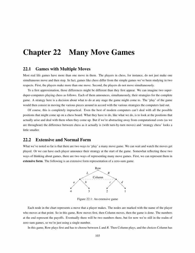
Chapter 22 Many Move Games

22.1 Games with Multiple MovesMost real life games have more than one move in them. The players in chess, for instance, do not just make one

simultaneous move and then stop. In fact, games like chess differ from the simple games we’ve been studying in two

respects. First, the players make more than one move. Second, the players do not move simultaneously.

To a first approximation, those differences might be different than they first appear. We can imagine two super-

duper-computers playing chess as follows. Each of them announces, simultaneously, their strategies for the complete

game. A strategy here is a decision about what to do at any stage the game might come to. The ‘play’ of the game

would then consist in moving the various pieces around in accord with the various strategies the computers laid out.

Of course, this is completely impractical. Even the best of modern computers can’t deal with all the possible

positions that might come up on a chess board. What they have to do, like what we do, is to look at the positions that

actually arise and deal with them when they come up. But if we’re abstracting away from computational costs (as we

are throughout) the difference between chess as it actually is (with turn-by-turn moves) and ‘strategy chess’ looks a

little smaller.

22.2 Extensive and Normal FormWhat we’ve noted so far is that there are two ways to ‘play’ a many move game. We can wait and watch the moves get

played. Or we can have each player announce their strategy at the start of the game. Somewhat reflecting these two

ways of thinking about games, there are two ways of representing many move games. First, we can represent them in

extensive form. The following is an extensive form representation of a zero-sum game.

b��

��

HHHHHH

Row

L Rr��

@@@

a br4

r3

r�

��

@@@

c dr2

r1

p p p p p p p p p p p p p p p p p p p pColumn

Figure 22.1: An extensive game

Each node in the chart represents a move that a player makes. The nodes are marked with the name of the player

who moves at that point. So in this game, Row moves first, then Column moves, then the game is done. The numbers

at the end represent the payoffs. Eventually there will be two numbers there, but for now we’re still in the realm of

zero-sum games, so we’re just using a single number.

In this game, Row plays first and has to choose between L and R. Then Column plays, and the choices Column has

103

22.3 Two Types of Equilibrium 22. Many Move Games

depend on what move Row made. If Row played L, then Column could choose between a and b. (And presumably

would choose b, since Column is trying to minimise the number.) If Row played R, then Column could choose between

c and d. (And presumably would choose d, since Column is trying to minimise the number.) If we assume Column

will make the rational play, then Row’s choice is really between getting 3, if she plays L, and 1, if she plays R, so she

should play L.

As well as this extensive form representation, we can also represent the game in normal form. A normal form

representation is where we set out each player’s possible strategies for the game. As above, a strategy is a decision

about what to do in every possibility that may arise. Since Row only has one move in this game, her strategy is just

a matter of that first move. But Column’s strategy has to specify two things: what to do if Row plays L, and what to

do if Row plays R. We’ll represent a strategy for Column with two letters, e.g., ac. That’s the strategy of playing a if

Row plays L and c if Row plays R. The normal form of this game is then

ac ad bc bd

L 4 4 3 3

R 2 1 2 1

22.3 Two Types of EquilibriumIn the game we’ve been looking at above, there are two Nash equilibrium outcomes. The first is < L,bc >, and the

second is < L,bd >. Both of these end up with a payoff of 3. But there is something odd about the first equilibrium. In

that equilibrium, Column has a strategy that embeds some odd dispositions. If Row (foolishly) plays R, then Column’s

strategy says to (equally foolishly) play c. But clearly the best play for Column in this circumstance is d, not c.

So in a sense, < L,bc > is not an equilibrium strategy. True, it is as good as any strategy that Column can follow

given Row’s other choices. But it isn’t an optimal strategy for Column to follow with respect to every decision that

Column has to make.

We’ll say a subgame perfect equilibrium is a pair of strategies for Row and Column such that for any given

node in the game, from that node on, neither can do better given the other’s strategy. A Nash equilibrium satisfies this

condition for the ‘initial’ node; subgame perfect equilibrium requires that it be satisfied for all nodes.

22.4 Normative Significance of Subgame Perfect EquilibriumSubgame perfect equilibrium is a very significant concept in modern game theory. Some writers take it to be an

important restriction on rational action that players play strategies which are part of subgame perfect equilibria. But it

is a rather odd concept for a few reasons. We’ll say more about this after we stop restricting our attention to zero-sum

games, but for now, consider the game in Figure 22.2. (I’ve used R and C for Row and Column to save space. Again,

it’s a zero-sum game. And the initial node in these games is always the open circle; the closed circles are nodes that

we may or may not get to.)

Note that Row’s strategy has to include two choices: what to do at the first node, and what to do at the third node.

But Column has (at most) one choice. Note also that the game ends as soon as any player plays d. The game continues

as long as players are playing r, until there are 3 plays of r.

104

22. Many Move Games 22.5 Cooperative Games

bRd

r

r3

rrCd

r

r2

rrRd

r

r4

r 1

Figure 22.2: Illustrating subgame perfect equilibrium

We can work out the subgame perfect equilibrium by backwards induction from the terminal nodes of the game.

At the final node, the dominating option for Row is d, so Row should play d. Given that Row is going to play d at

that final choice-point, and hence end the game with 4, Column is better off playing d at her one and only choice, and

ending the game with 2 rather than the 4 it would end with if Row was allowed to play last. And given that that’s what

Column is planning to do, Row is better off ending the game straight away by playing d at the very first opportunity,

and ending with 3. So the subgame perfect equilibrium is < dd,d >.

There are three oddities about this game.

First, if Row plays d straight away, then the game is over and it doesn’t matter what the rest of the strategies are. So

there are many Nash equilibria for this game. That implies that there are Nash equilibria that are not subgame perfect

equilibria. For instance, < dr,d > is a Nash equilibria, but isn’t subgame perfect. That’s not, however, something we

haven’t seen before.

Second, the reason that < dr,d > is not an equilibrium is that it is an irrational thing for Row to play if the game

were to get to the third node. But if Row plays that very strategy, then the game won’t get to that third node. Oddly,

Row is being criticised here for playing a strategy that could, in principle, have a bad outcome, but will only have a

bad outcome if she doesn’t play that very strategy. So it isn’t clear that her strategy is so bad.

Finally, let’s think again about Column’s option at the middle node. We worked out what Column should do by

working backwards. But the game is played forwards. And if we reach that second node, where Column is playing,

then Column knows that Row is not playing an equilibrium strategy. Given that Column knows this, perhaps it isn’t

altogether obvious that Column should hold onto the assumption that Row is perfectly rational. But without the

assumption that Row is perfectly rational, then it isn’t obvious that Column should play d. After all, that’s only the

best move on the assumption that Row is rational.

The philosophical points here are rather tricky, and we’ll come back to them when we’ve looked more closely at

non zero sum games.

22.5 Cooperative GamesAs we’ve stressed several times, most human interactions are not zero sum. Most of the time, there is some opportunity

for the players’ interests to be aligned. This is so even when we look at games involving one (simultaneous) move.

We won’t prove this, but it turns out that even when we drop the restriction to zero-sum games, every game has a

Nash equilibrium. Sometimes this will be a mixed strategy equilibrium, but often it will be a pure strategy. What is

surprising about non-zero sum games is that it is possible for there to be multiple Nash equilibria that are not equal in

their outcomes. For instance, consider the following game.

105

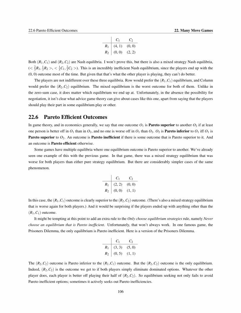
22.6 Pareto Efficient Outcomes 22. Many Move Games

C1 C2

R1 (4, 1) (0, 0)

R2 (0, 0) (2, 2)

Both (R1,C1) and (R2,C2) are Nash equilibria. I won’t prove this, but there is also a mixed strategy Nash equilibria,

(< 23 R1,

13 R2 >, < 1

3C1,23C2 >). This is an incredibly inefficient Nash equilibrium, since the players end up with the

(0, 0) outcome most of the time. But given that that’s what the other player is playing, they can’t do better.

The players are not indifferent over these three equilibria. Row would prefer the (R1,C1) equilibrium, and Column

would prefer the (R2,C2) equilibrium. The mixed equilibrium is the worst outcome for both of them. Unlike in

the zero-sum case, it does matter which equilibrium we end up at. Unfortunately, in the absence the possibility for

negotiation, it isn’t clear what advice game theory can give about cases like this one, apart from saying that the players

should play their part in some equilibrium play or other.

22.6 Pareto Efficient OutcomesIn game theory, and in economics generally, we say that one outcome O1 is Pareto superior to another O2 if at least

one person is better off in O1 than in O2, and no one is worse off in O1 than O2. O2 is Pareto inferior to O1 iff O1 is

Pareto superior to O2. An outcome is Pareto inefficient if there is some outcome that is Pareto superior to it. And

an outcome is Pareto efficient otherwise.

Some games have multiple equilibria where one equilibrium outcome is Pareto superior to another. We’ve already

seen one example of this with the previous game. In that game, there was a mixed strategy equilibrium that was

worse for both players than either pure strategy equilibrium. But there are considerably simpler cases of the same

phenomenon.

C1 C2

R1 (2, 2) (0, 0)

R2 (0, 0) (1, 1)

In this case, the (R1,C1) outcome is clearly superior to the (R2,C2) outcome. (There’s also a mixed strategy equilibrium

that is worse again for both players.) And it would be surprising if the players ended up with anything other than the

(R1,C1) outcome.

It might be tempting at this point to add an extra rule to the Only choose equilibrium strategies rule, namely Never

choose an equilibrium that is Pareto inefficient. Unfortunately, that won’t always work. In one famous game, the

Prisoners Dilemma, the only equilibrium is Pareto inefficient. Here is a version of the Prisoners Dilemma.

C1 C2

R1 (3, 3) (5, 0)

R2 (0, 5) (1, 1)

The (R2,C2) outcome is Pareto inferior to the (R1,C1) outcome. But the (R2,C2) outcome is the only equilibrium.

Indeed, (R2,C2) is the outcome we get to if both players simply eliminate dominated options. Whatever the other

player does, each player is better off playing their half of (R2,C2). So equilibrium seeking not only fails to avoid

Pareto inefficient options; sometimes it actively seeks out Pareto inefficiencies.

106

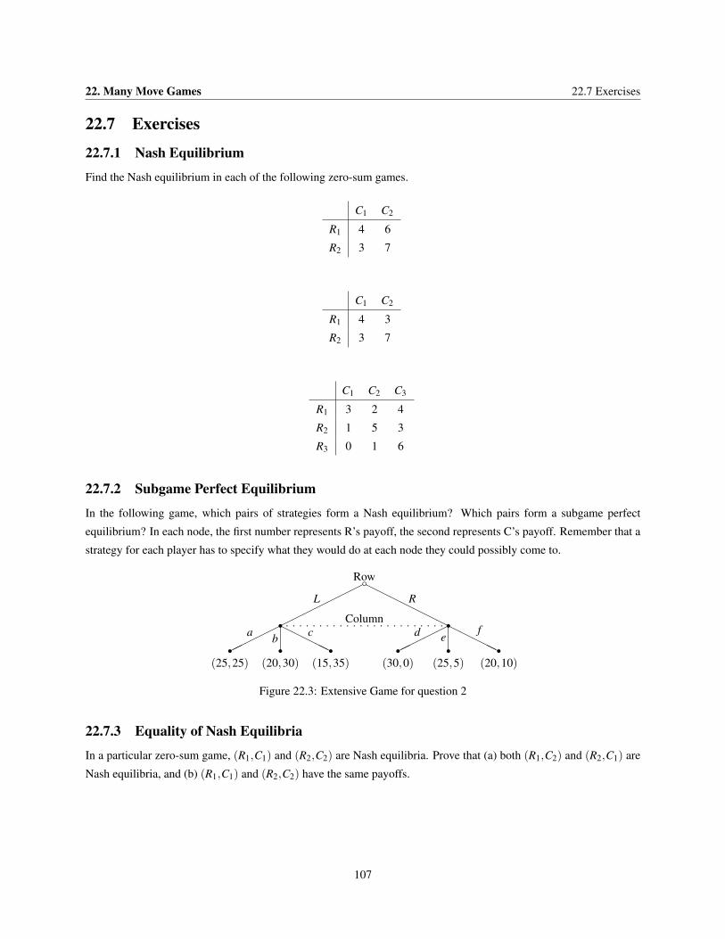
22. Many Move Games 22.7 Exercises

22.7 Exercises

22.7.1 Nash Equilibrium

Find the Nash equilibrium in each of the following zero-sum games.

C1 C2

R1 4 6

R2 3 7

C1 C2

R1 4 3

R2 3 7

C1 C2 C3

R1 3 2 4

R2 1 5 3

R3 0 1 6

22.7.2 Subgame Perfect Equilibrium

In the following game, which pairs of strategies form a Nash equilibrium? Which pairs form a subgame perfect

equilibrium? In each node, the first number represents R’s payoff, the second represents C’s payoff. Remember that a

strategy for each player has to specify what they would do at each node they could possibly come to.

b��

��

HHHH

HHH

Row

L Rr��

HHHHH

a b cr(25,25)

r(20,30)

r(15,35)

r��

HHHHH

d efr

(30,0)r

(25,5)r

(20,10)

p p p p p p p p p p p p p p p p p p p p p p p p pColumn

Figure 22.3: Extensive Game for question 2

22.7.3 Equality of Nash Equilibria

In a particular zero-sum game, (R1,C1) and (R2,C2) are Nash equilibria. Prove that (a) both (R1,C2) and (R2,C1) are

Nash equilibria, and (b) (R1,C1) and (R2,C2) have the same payoffs.

107

22.7 Exercises 22. Many Move Games

108

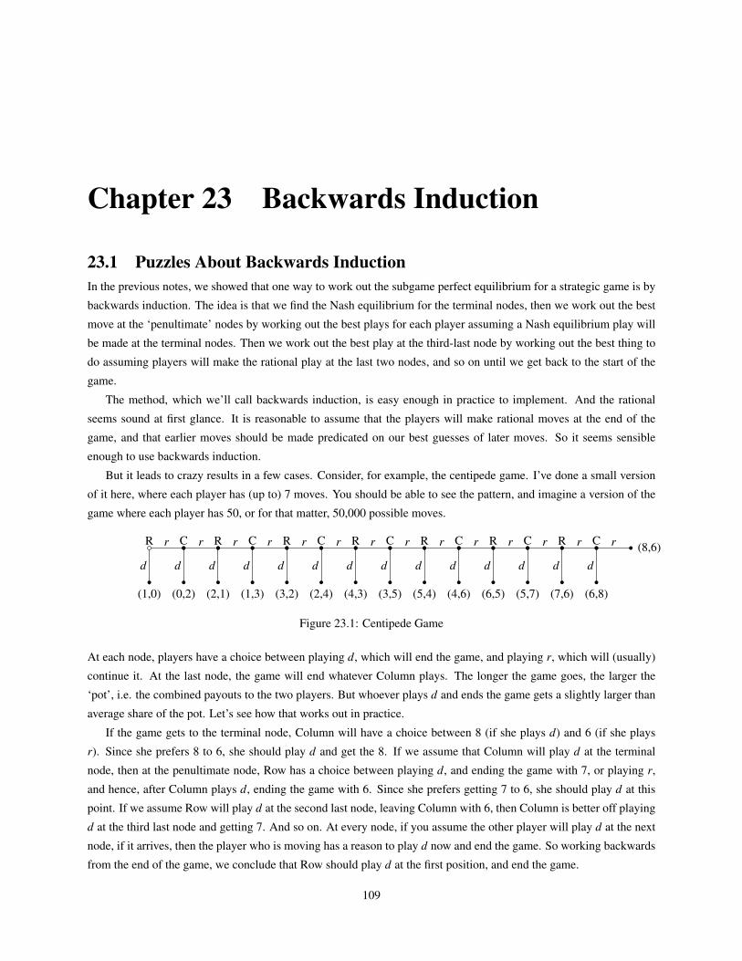
Chapter 23 Backwards Induction

23.1 Puzzles About Backwards InductionIn the previous notes, we showed that one way to work out the subgame perfect equilibrium for a strategic game is by

backwards induction. The idea is that we find the Nash equilibrium for the terminal nodes, then we work out the best

move at the ‘penultimate’ nodes by working out the best plays for each player assuming a Nash equilibrium play will

be made at the terminal nodes. Then we work out the best play at the third-last node by working out the best thing to

do assuming players will make the rational play at the last two nodes, and so on until we get back to the start of the

game.

The method, which we’ll call backwards induction, is easy enough in practice to implement. And the rational

seems sound at first glance. It is reasonable to assume that the players will make rational moves at the end of the

game, and that earlier moves should be made predicated on our best guesses of later moves. So it seems sensible

enough to use backwards induction.

But it leads to crazy results in a few cases. Consider, for example, the centipede game. I’ve done a small version

of it here, where each player has (up to) 7 moves. You should be able to see the pattern, and imagine a version of the

game where each player has 50, or for that matter, 50,000 possible moves.

bRd

r

r(1,0)

rrCd

r

r(0,2)

rrRd

r

r(2,1)

rrCd

r

r(1,3)

rrRd

r

r(3,2)

rrCd

r

r(2,4)

rrRd

r

r(4,3)

rrCd

r

r(3,5)

rrRd

r

r(5,4)

rrCd

r

r(4,6)

rrRd

r

r(6,5)

rrCd

r

r(5,7)

rrRd

r

r(7,6)

rrCd

r

r(6,8)

r (8,6)

Figure 23.1: Centipede Game

At each node, players have a choice between playing d, which will end the game, and playing r, which will (usually)

continue it. At the last node, the game will end whatever Column plays. The longer the game goes, the larger the

‘pot’, i.e. the combined payouts to the two players. But whoever plays d and ends the game gets a slightly larger than

average share of the pot. Let’s see how that works out in practice.

If the game gets to the terminal node, Column will have a choice between 8 (if she plays d) and 6 (if she plays

r). Since she prefers 8 to 6, she should play d and get the 8. If we assume that Column will play d at the terminal

node, then at the penultimate node, Row has a choice between playing d, and ending the game with 7, or playing r,

and hence, after Column plays d, ending the game with 6. Since she prefers getting 7 to 6, she should play d at this

point. If we assume Row will play d at the second last node, leaving Column with 6, then Column is better off playing

d at the third last node and getting 7. And so on. At every node, if you assume the other player will play d at the next

node, if it arrives, then the player who is moving has a reason to play d now and end the game. So working backwards

from the end of the game, we conclude that Row should play d at the first position, and end the game.

109

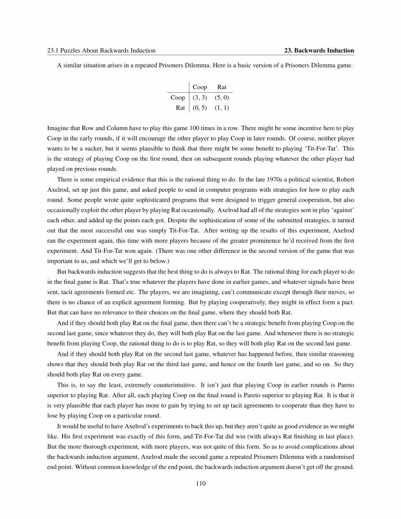
23.1 Puzzles About Backwards Induction 23. Backwards Induction

A similar situation arises in a repeated Prisoners Dilemma. Here is a basic version of a Prisoners Dilemma game.

Coop Rat

Coop (3, 3) (5, 0)

Rat (0, 5) (1, 1)

Imagine that Row and Column have to play this game 100 times in a row. There might be some incentive here to play

Coop in the early rounds, if it will encourage the other player to play Coop in later rounds. Of course, neither player

wants to be a sucker, but it seems plausible to think that there might be some benefit to playing ‘Tit-For-Tat’. This

is the strategy of playing Coop on the first round, then on subsequent rounds playing whatever the other player had

played on previous rounds.

There is some empirical evidence that this is the rational thing to do. In the late 1970s a political scientist, Robert

Axelrod, set up just this game, and asked people to send in computer programs with strategies for how to play each

round. Some people wrote quite sophisticated programs that were designed to trigger general cooperation, but also

occasionally exploit the other player by playing Rat occasionally. Axelrod had all of the strategies sent in play ‘against’

each other, and added up the points each got. Despite the sophistication of some of the submitted strategies, it turned

out that the most successful one was simply Tit-For-Tat. After writing up the results of this experiment, Axelrod

ran the experiment again, this time with more players because of the greater prominence he’d received from the first

experiment. And Tit-For-Tat won again. (There was one other difference in the second version of the game that was

important to us, and which we’ll get to below.)

But backwards induction suggests that the best thing to do is always to Rat. The rational thing for each player to do

in the final game is Rat. That’s true whatever the players have done in earlier games, and whatever signals have been

sent, tacit agreements formed etc. The players, we are imagining, can’t communicate except through their moves, so

there is no chance of an explicit agreement forming. But by playing cooperatively, they might in effect form a pact.

But that can have no relevance to their choices on the final game, where they should both Rat.

And if they should both play Rat on the final game, then there can’t be a strategic benefit from playing Coop on the

second last game, since whatever they do, they will both play Rat on the last game. And whenever there is no strategic

benefit from playing Coop, the rational thing to do is to play Rat, so they will both play Rat on the second last game.

And if they should both play Rat on the second last game, whatever has happened before, then similar reasoning

shows that they should both play Rat on the third last game, and hence on the fourth last game, and so on. So they

should both play Rat on every game.

This is, to say the least, extremely counterintuitive. It isn’t just that playing Coop in earlier rounds is Pareto

superior to playing Rat. After all, each playing Coop on the final round is Pareto superior to playing Rat. It is that it

is very plausible that each player has more to gain by trying to set up tacit agreements to cooperate than they have to

lose by playing Coop on a particular round.

It would be useful to have Axelrod’s experiments to back this up, but they aren’t quite as good evidence as we might

like. His first experiment was exactly of this form, and Tit-For-Tat did win (with always Rat finishing in last place).

But the more thorough experiment, with more players, was not quite of this form. So as to avoid complications about

the backwards induction argument, Axelrod made the second game a repeated Prisoners Dilemma with a randomised

end point. Without common knowledge of the end point, the backwards induction argument doesn’t get off the ground.

110

23. Backwards Induction 23.2 Pettit and Sugden

Still, it seems highly implausible that rationality requires us to play Rat at every stage, or to play d at every stage

in the Centipede game. In the next section we’ll look at an argument by Philip Pettit and Robert Sugden that suggests

this is not a requirement of rationality.

23.2 Pettit and SugdenThe backwards induction reasoning is, as the name suggests, from the back of the game to the front of it. But games

are played from front to back, and we should check how the reasoning looks from this perspective. For simplicity,

we’ll work with Centipede, though what we say should carry over to finitely iterated Prisoners Dilemma as well.

First, imagine that one of the players does not play the subgame perfect equilibrium solution to the game. So

imagine that Row plays r at the first move. Now Column has a choice to make at the second node. Column knows

that if Row plays the subgame perfect equilibrium at the third move, then the best thing for her to do now is to play d.

And Column presupposed, at the start of the game, that Row was rational. And we’re supposing, so far, that rational

players play subgame perfect equilibrium plays. So Column should play d right?

Not necessarily. At the start of the game, Column assumed that Row was a rational player. But Row has given her

evidence, irrefutable evidence given our assumption that rationality equals making subgame perfect equilibrium plays,

that she is not rational. And it isn’t at all clear that the right thing to do when playing with a less than rational player

is to play d. If there is even a small chance that they will keep playing r, then it is probably worthwhile to give them

the chance to do so.

That’s all to say, given the assumptions that we made, if Row plays r, Column might well reciprocate by playing

r. But if that’s true, then there is no reason for Row to play d at the start. The argument that Row should play d turned

on the assumption that if she played r, Column would play d. And given various assumptions we made at the start of

the game, Column would have played d. But, and here is the crucial point, if Column were in a position to make a

move at all, those assumptions would no longer still be operational. So perhaps it is rational for Row to play r.

None of this is to say that Row should play r on her last move. After all, whatever Column thinks about Row’s

rationality, Column will play d on the last move, so Row should play d if it gets to her last move. It isn’t even clear that

it gives Row or Column a reason to play r on their second last moves, since even then it isn’t clear there is a strategic

benefit to be had. But it might given them a reason to play r on earlier moves, as was intuitively plausible.

There is something that might seem odd about this whole line of reasoning. We started off saying that the uniquely

rational option was to play d everywhere. We then said that if Row played r, Column wouldn’t think that Row was

rational, so all bets were off with respect to backwards induction reasoning. So it might be sensible for Row to play r.

Now you might worry that if all that’s true, then when Row plays r, that won’t be a sign that Row is irrational. Indeed,

it will be a sign that Row is completely rational! So how can Pettit and Sugden argue that Column won’t play d at the

second node?

Well, if their reasoning is right that r is a rational move at the initial node, then it is also good reasoning that

Column can play r at the second node. Either playing r early in the game is rational or it isn’t. If it is, then both

players can play r for a while as a rational resolution of the game. If it isn’t, then Row can play r as a way of signaling

that she is irrational, and hence Column has some reason to play r. Either way, the players can keep on playing r.

The upshot of this is that backwards induction reasoning is less impressive than it looked at first.

111

23.2 Pettit and Sugden 23. Backwards Induction

112

Chapter 24 Group DecisionsSo far, we’ve been looking at the way that an individual may make a decision. In practice, we are just as often

concerned with group decisions as with individual decisions. These range from relatively trivial concerns (e.g. Which

movie shall we see tonight?) to some of the most important decisions we collectively make (e.g. Who shall be the

next President?). So methods for grouping individual judgments into a group decision seem important.

Unfortunately, it turns out that there are several challenges facing any attempt to merge preferences into a single

decision. In this chapter, we’ll look at various approaches that different groups take to form decisions, and how

these different methods may lead to different results. The different methods have different strengths and, importantly,

different weaknesses. We might hope that there would be a method with none of these weaknesses. Unfortunately,

this turns out to be impossible.

One of the most important results in modern decision theory is the Arrow Impossibility Theorem, named after

the economist Kenneth Arrow who discovered it. The Arrow Impossibility Theorem says that there is no method for

making group decisions that satisfies a certain, relatively small, list of desiderata. The next chapter will set out the

theorem, and explore a little what those constraints are.

Finally, we’ll look a bit at real world voting systems, and their different strengths and weaknesses. Different

democracies use quite different voting systems to determine the winner of an election. (Indeed, within the United

States there is an interesting range of systems used.) And some theorists have promoted the use of yet other systems

than are currently used. Choosing a voting system is not quite like choosing a method for making a group decision.

For the next two chapters, when we’re looking at ways to aggregate individual preferences into a group decision,

we’ll assume that we have clear access to the preferences of individual agents. A voting system is not meant to tally

preferences into a decision, it is meant to tally votes. And voters may have reasons (some induced by the system itself)

for voting in ways other than their preferences. For instance, many voters in American presidential elections vote for

their preferred candidate of the two major candidates, rather than ‘waste’ their vote on a third party candidate.

For now we’ll put those problems to one side, and assume that members of the group express themselves honestly

when voting. Still, it turns out there are complications that arise for even relatively simple decisions.

24.1 Making a DecisionSeven friends, who we’ll imaginatively name F1,F2, ...,F7 are trying to decide which restaurant to go to. They have

four options, which we’ll also imaginatively name R1,R2,R3,R4. The first thing they do is ask which restaurant each

person prefers. The results are as follows.

• F1,F2 and F3 all vote for R1, so it gets 3 votes

• F4 and F5 both vote for R2, so it gets 2 votes

• F6 votes for R3, so it gets 1 vote

113

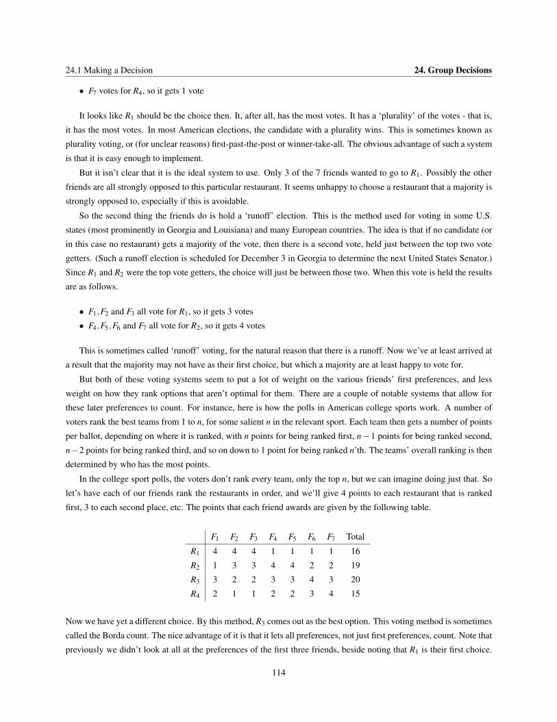
24.1 Making a Decision 24. Group Decisions

• F7 votes for R4, so it gets 1 vote

It looks like R1 should be the choice then. It, after all, has the most votes. It has a ‘plurality’ of the votes - that is,

it has the most votes. In most American elections, the candidate with a plurality wins. This is sometimes known as

plurality voting, or (for unclear reasons) first-past-the-post or winner-take-all. The obvious advantage of such a system

is that it is easy enough to implement.

But it isn’t clear that it is the ideal system to use. Only 3 of the 7 friends wanted to go to R1. Possibly the other

friends are all strongly opposed to this particular restaurant. It seems unhappy to choose a restaurant that a majority is

strongly opposed to, especially if this is avoidable.

So the second thing the friends do is hold a ‘runoff’ election. This is the method used for voting in some U.S.

states (most prominently in Georgia and Louisiana) and many European countries. The idea is that if no candidate (or

in this case no restaurant) gets a majority of the vote, then there is a second vote, held just between the top two vote

getters. (Such a runoff election is scheduled for December 3 in Georgia to determine the next United States Senator.)

Since R1 and R2 were the top vote getters, the choice will just be between those two. When this vote is held the results

are as follows.

• F1,F2 and F3 all vote for R1, so it gets 3 votes

• F4,F5,F6 and F7 all vote for R2, so it gets 4 votes

This is sometimes called ‘runoff’ voting, for the natural reason that there is a runoff. Now we’ve at least arrived at

a result that the majority may not have as their first choice, but which a majority are at least happy to vote for.

But both of these voting systems seem to put a lot of weight on the various friends’ first preferences, and less

weight on how they rank options that aren’t optimal for them. There are a couple of notable systems that allow for

these later preferences to count. For instance, here is how the polls in American college sports work. A number of

voters rank the best teams from 1 to n, for some salient n in the relevant sport. Each team then gets a number of points

per ballot, depending on where it is ranked, with n points for being ranked first, n−1 points for being ranked second,

n−2 points for being ranked third, and so on down to 1 point for being ranked n’th. The teams’ overall ranking is then

determined by who has the most points.

In the college sport polls, the voters don’t rank every team, only the top n, but we can imagine doing just that. So

let’s have each of our friends rank the restaurants in order, and we’ll give 4 points to each restaurant that is ranked

first, 3 to each second place, etc. The points that each friend awards are given by the following table.

F1 F2 F3 F4 F5 F6 F7 Total

R1 4 4 4 1 1 1 1 16

R2 1 3 3 4 4 2 2 19

R3 3 2 2 3 3 4 3 20

R4 2 1 1 2 2 3 4 15

Now we have yet a different choice. By this method, R3 comes out as the best option. This voting method is sometimes

called the Borda count. The nice advantage of it is that it lets all preferences, not just first preferences, count. Note that

previously we didn’t look at all at the preferences of the first three friends, beside noting that R1 is their first choice.

114

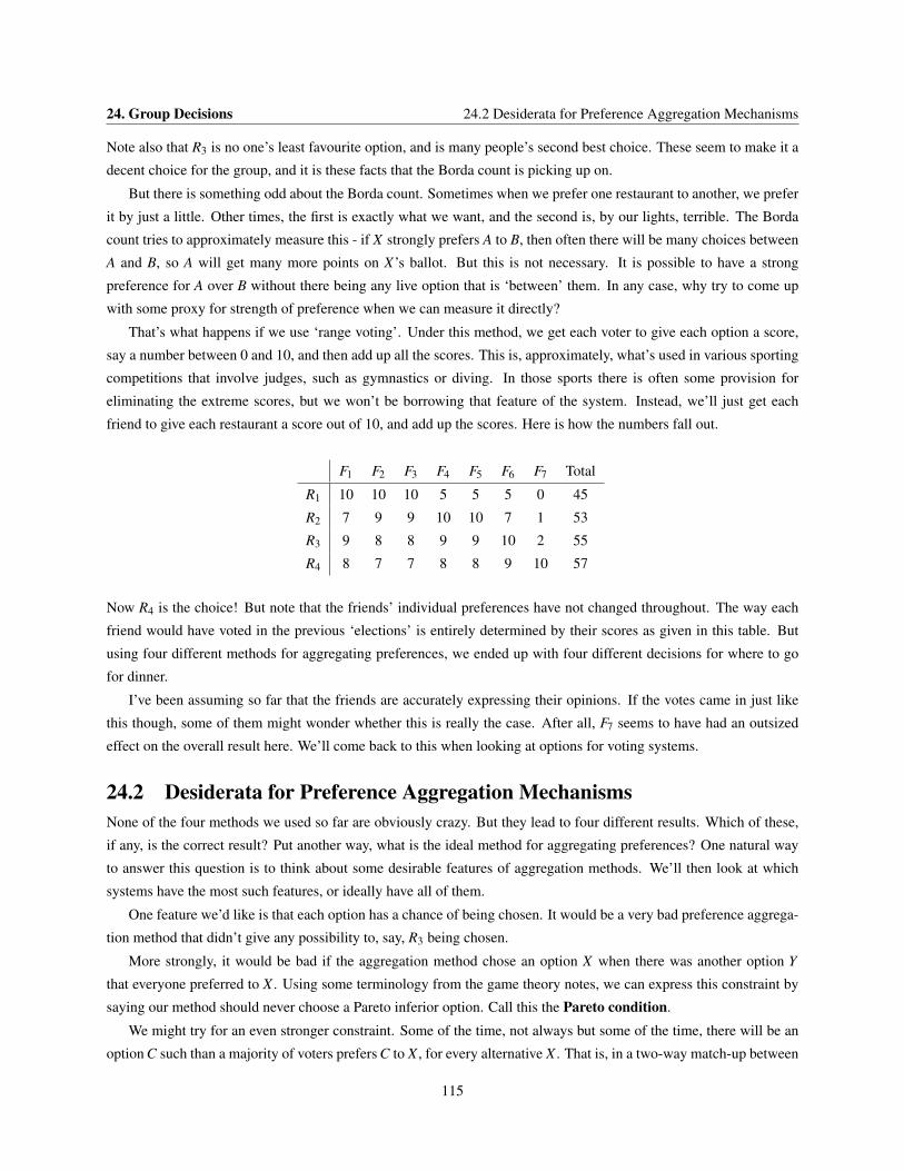
24. Group Decisions 24.2 Desiderata for Preference Aggregation Mechanisms

Note also that R3 is no one’s least favourite option, and is many people’s second best choice. These seem to make it a

decent choice for the group, and it is these facts that the Borda count is picking up on.

But there is something odd about the Borda count. Sometimes when we prefer one restaurant to another, we prefer

it by just a little. Other times, the first is exactly what we want, and the second is, by our lights, terrible. The Borda

count tries to approximately measure this - if X strongly prefers A to B, then often there will be many choices between

A and B, so A will get many more points on X’s ballot. But this is not necessary. It is possible to have a strong

preference for A over B without there being any live option that is ‘between’ them. In any case, why try to come up

with some proxy for strength of preference when we can measure it directly?

That’s what happens if we use ‘range voting’. Under this method, we get each voter to give each option a score,

say a number between 0 and 10, and then add up all the scores. This is, approximately, what’s used in various sporting

competitions that involve judges, such as gymnastics or diving. In those sports there is often some provision for

eliminating the extreme scores, but we won’t be borrowing that feature of the system. Instead, we’ll just get each

friend to give each restaurant a score out of 10, and add up the scores. Here is how the numbers fall out.

F1 F2 F3 F4 F5 F6 F7 Total

R1 10 10 10 5 5 5 0 45

R2 7 9 9 10 10 7 1 53

R3 9 8 8 9 9 10 2 55

R4 8 7 7 8 8 9 10 57

Now R4 is the choice! But note that the friends’ individual preferences have not changed throughout. The way each

friend would have voted in the previous ‘elections’ is entirely determined by their scores as given in this table. But

using four different methods for aggregating preferences, we ended up with four different decisions for where to go

for dinner.

I’ve been assuming so far that the friends are accurately expressing their opinions. If the votes came in just like

this though, some of them might wonder whether this is really the case. After all, F7 seems to have had an outsized

effect on the overall result here. We’ll come back to this when looking at options for voting systems.

24.2 Desiderata for Preference Aggregation MechanismsNone of the four methods we used so far are obviously crazy. But they lead to four different results. Which of these,

if any, is the correct result? Put another way, what is the ideal method for aggregating preferences? One natural way

to answer this question is to think about some desirable features of aggregation methods. We’ll then look at which

systems have the most such features, or ideally have all of them.

One feature we’d like is that each option has a chance of being chosen. It would be a very bad preference aggrega-

tion method that didn’t give any possibility to, say, R3 being chosen.

More strongly, it would be bad if the aggregation method chose an option X when there was another option Y

that everyone preferred to X . Using some terminology from the game theory notes, we can express this constraint by

saying our method should never choose a Pareto inferior option. Call this the Pareto condition.

We might try for an even stronger constraint. Some of the time, not always but some of the time, there will be an

option C such than a majority of voters prefers C to X , for every alternative X . That is, in a two-way match-up between

115

24.3 Assessing Plurality Voting 24. Group Decisions

C and any other option X , C will get more votes. Such an option is sometimes called a Condorcet option, after Marie

Jean Antoine Nicolas Caritat, the Marquis de Condorcet, who discussed such options. The Condorcet condition on

aggregation methods is that a Condorcet option always comes first, if such an option exists.

Moving away from these comparative norms, we might also want our preference aggregation system to be fair

to everyone. A method that said F2 is the dictator, and F2’s preferences are the group’s preferences, would deliver a

clear answer, but does not seem to be particularly fair to the group. There should be no dictators; for any person, it is

possible that the group’s decision does not match up with their preference.

More generally than that, we might restrict attention to preference aggregation systems that don’t pay attention to

who has various preferences, just to what preferences people have. Here’s one way of stating this formally. Assume

that two members of the group, v1 and v2, swap preferences, so v1’s new preference ordering is v2’s old preference

ordering and vice versa. This shouldn’t change what the group’s decision is, since from a group level, nothing has

changed. Call this the symmetry condition.

Finally, we might want to impose a condition that we said is a condition we imposed on independent agents: the

irrelevance of independent alternatives. If the group would choose A when the options are A and B, then they

wouldn’t choose B out of any larger set of options that also include A. More generally, adding options can change the

group’s choice, but only to one of the new options.

24.3 Assessing Plurality VotingIt is perhaps a little disturbing to think how few of those conditions are met by plurality voting, which is how Presidents

of the USA are elected. Plurality voting clearly satisfies the Pareto condition. If everyone prefers A to B, then B will

get no votes, and so won’t win. So far so good. And since any one person might be the only person who votes for their

preferred candidate, and since other candidates might get more than one vote, no one person can dictate who wins. So

it satisfies no dictators. Finally, since the system only looks at votes, and not at who cast them, it satisfies symmetry.

But it does not satisfy the Condorcet condition. Consider an election with three candidates. A gets 40% of the

vote, B gets 35% of the vote, and C gets 25% of the vote. A wins, and C doesn’t even finish second. But assume also

that everyone who didn’t vote for C has her as their second preference after either A or B. Something like this may

happen if, for instance, C is an independent moderate, and A and B are doctrinaire candidates from the major parties.

Then 60% prefer C to A, and 65% prefer C to B. So C is a Condorcet candidate, yet is not elected.

A similar example shows that the system does not satisfy the irrelevance of independent alternatives condition.

If B was not running, then presumably A would still have 40% of the vote, while C would have 60% of the vote,

and would win. One thing you might want to think about is how many elections in recent times would have had the

outcome changed by eliminating (or adding) unsuccessful candidates in this way.

116

Chapter 25 Arrow’s Theorem

25.1 Ranking FunctionsThe purpose of this chapter is to set out Arrow’s Theorem, and its implications for the construction of group preferences

from individual preferences. We’ll also say a little about the implications of the theorem for the design of voting

systems, though we’ll leave most of that to the next chapter.

The theorem is a mathematical result, and needs careful setup. We’ll assume that each agent has a complete and

transitive preference ordering over the options. If we say A >V B means that V prefers A to B, that A =V B means

that V is indifferent between A and B, and that A ≥V B means that A >V B∨A =V B, then these constraints can be

expressed as follows.

Completeness For any voter V and options A,B, either A≥V B or B≥V A

Transitivity For any voter V and options A,B, the following three conditions hold:

• If A >V B and B >V C then A >V C

• If A =V B and B =V C then A =V C

• If A≥V B and B≥V C then A≥V C

More generally, we assume the substitutivity of indifferent options. That is, if A =V B, then whatever is true of the

agent’s attitude towards A is also true of the agent’s attitude towards B. In particular, whatever comparison holds in

the agent’s mind between A and C holds between B and C. (The last two bullet points under transitivity follow from

this principle about indifference and the earlier bullet point.)

The effect of these assumptions is that we can represent the agent’s preferences by lining up the options from best

to worst, with the possibility that we’ll have to put two options in one ‘spot’ to represent the fact that the agent values

each of them equally.

A ranking function is a function from the preference orderings of the agent to a new preference ordering, which

we’ll call the preference ordering of the group. We’ll use the subscript G to note that it is the group’s ordering we are

designing. We’ll also assume that the group’s preference ordering is complete and transitive.

There are any number ranking functions that don’t look at all like the group’s preferences in any way. For instance,

if the function is meant to work out the results of an election, we could consider the function that takes any input

whatsoever, and returns a ranking that simply lists by age, with the oldest first, the second oldest second, etc. This

doesn’t seem like it is the group’s preferences in any way. Whatever any member of the group thinks, the oldest

candidate wins. What Arrow called the citizen sovereignty condition is that for any possible ranking, it should be

possible to have the group end up with that ranking.

117

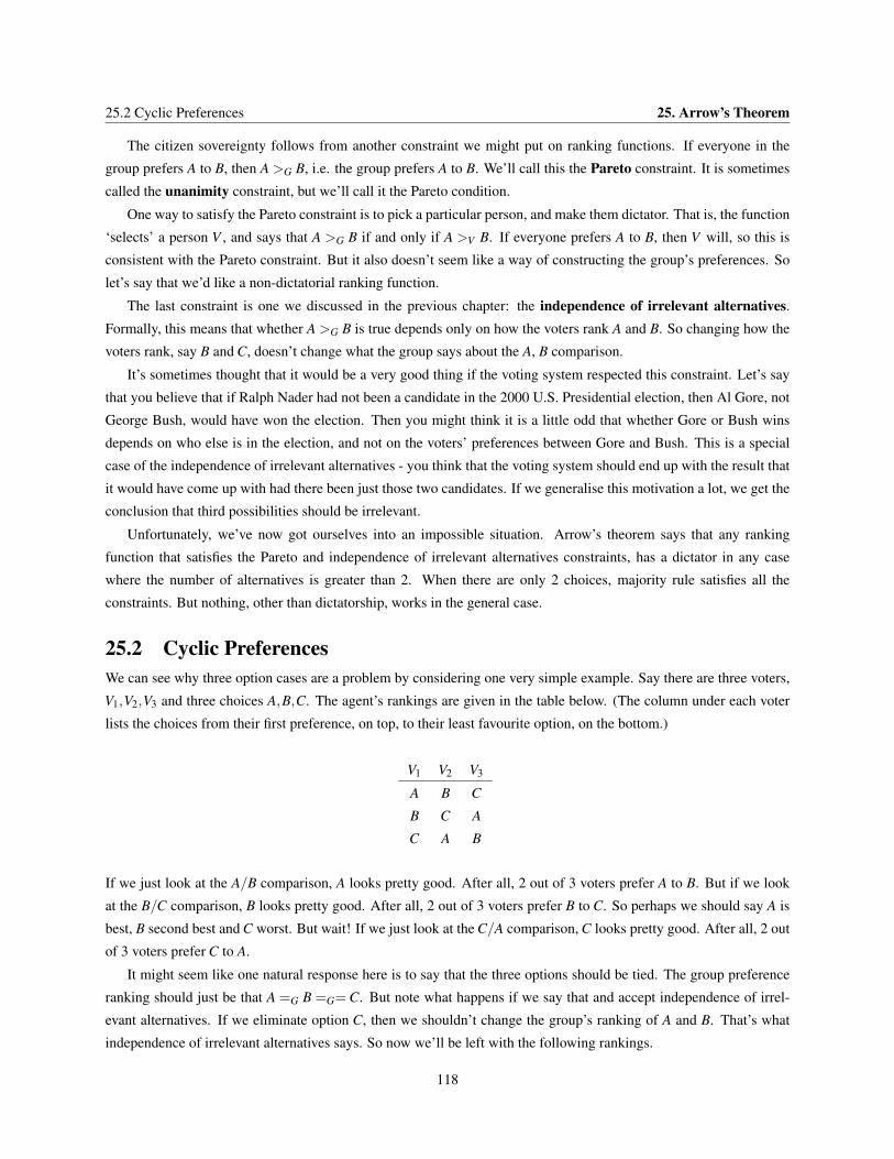
25.2 Cyclic Preferences 25. Arrow’s Theorem

The citizen sovereignty follows from another constraint we might put on ranking functions. If everyone in the

group prefers A to B, then A >G B, i.e. the group prefers A to B. We’ll call this the Pareto constraint. It is sometimes

called the unanimity constraint, but we’ll call it the Pareto condition.

One way to satisfy the Pareto constraint is to pick a particular person, and make them dictator. That is, the function

‘selects’ a person V , and says that A >G B if and only if A >V B. If everyone prefers A to B, then V will, so this is

consistent with the Pareto constraint. But it also doesn’t seem like a way of constructing the group’s preferences. So

let’s say that we’d like a non-dictatorial ranking function.

The last constraint is one we discussed in the previous chapter: the independence of irrelevant alternatives.

Formally, this means that whether A >G B is true depends only on how the voters rank A and B. So changing how the

voters rank, say B and C, doesn’t change what the group says about the A, B comparison.

It’s sometimes thought that it would be a very good thing if the voting system respected this constraint. Let’s say

that you believe that if Ralph Nader had not been a candidate in the 2000 U.S. Presidential election, then Al Gore, not

George Bush, would have won the election. Then you might think it is a little odd that whether Gore or Bush wins

depends on who else is in the election, and not on the voters’ preferences between Gore and Bush. This is a special

case of the independence of irrelevant alternatives - you think that the voting system should end up with the result that

it would have come up with had there been just those two candidates. If we generalise this motivation a lot, we get the

conclusion that third possibilities should be irrelevant.

Unfortunately, we’ve now got ourselves into an impossible situation. Arrow’s theorem says that any ranking

function that satisfies the Pareto and independence of irrelevant alternatives constraints, has a dictator in any case

where the number of alternatives is greater than 2. When there are only 2 choices, majority rule satisfies all the

constraints. But nothing, other than dictatorship, works in the general case.

25.2 Cyclic PreferencesWe can see why three option cases are a problem by considering one very simple example. Say there are three voters,

V1,V2,V3 and three choices A,B,C. The agent’s rankings are given in the table below. (The column under each voter

lists the choices from their first preference, on top, to their least favourite option, on the bottom.)

V1 V2 V3

A B C

B C A

C A B

If we just look at the A/B comparison, A looks pretty good. After all, 2 out of 3 voters prefer A to B. But if we look

at the B/C comparison, B looks pretty good. After all, 2 out of 3 voters prefer B to C. So perhaps we should say A is

best, B second best and C worst. But wait! If we just look at the C/A comparison, C looks pretty good. After all, 2 out

of 3 voters prefer C to A.

It might seem like one natural response here is to say that the three options should be tied. The group preference

ranking should just be that A =G B =G= C. But note what happens if we say that and accept independence of irrel-

evant alternatives. If we eliminate option C, then we shouldn’t change the group’s ranking of A and B. That’s what

independence of irrelevant alternatives says. So now we’ll be left with the following rankings.

118

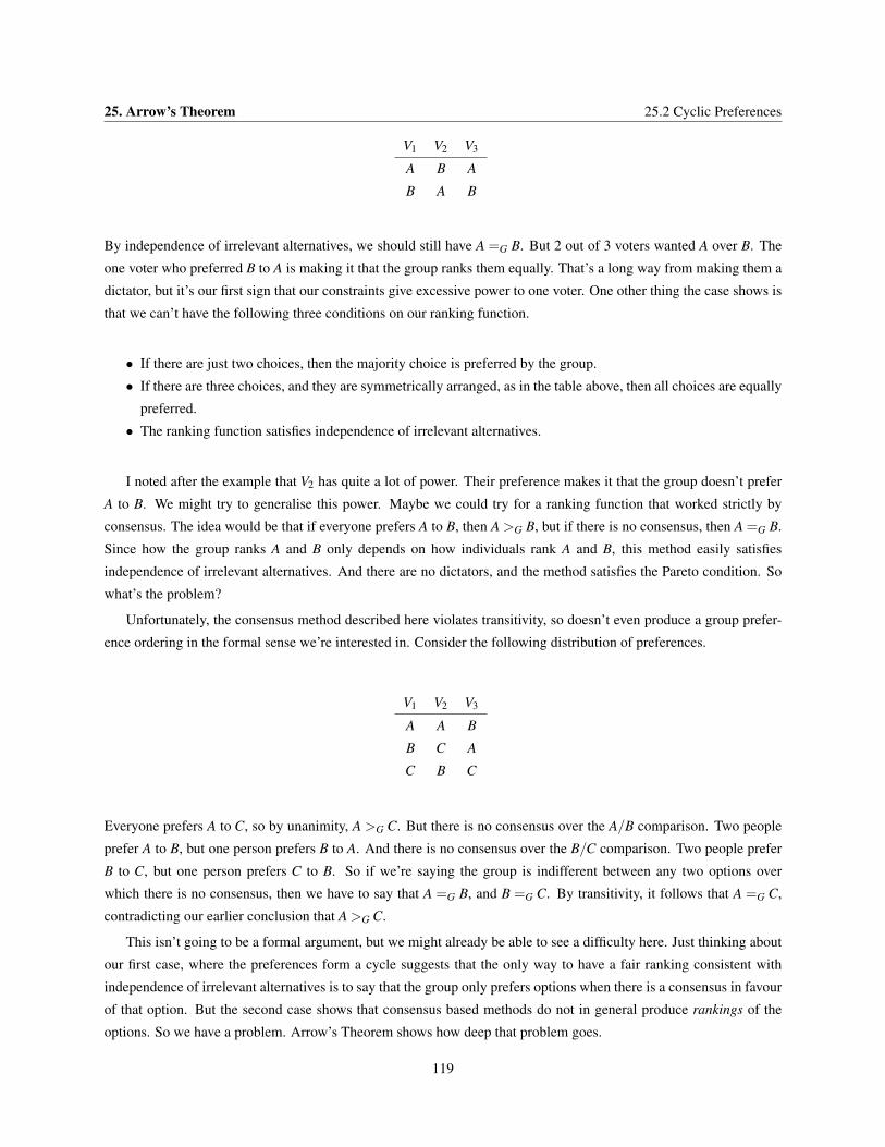
25. Arrow’s Theorem 25.2 Cyclic Preferences

V1 V2 V3

A B A

B A B

By independence of irrelevant alternatives, we should still have A =G B. But 2 out of 3 voters wanted A over B. The

one voter who preferred B to A is making it that the group ranks them equally. That’s a long way from making them a

dictator, but it’s our first sign that our constraints give excessive power to one voter. One other thing the case shows is

that we can’t have the following three conditions on our ranking function.

• If there are just two choices, then the majority choice is preferred by the group.

• If there are three choices, and they are symmetrically arranged, as in the table above, then all choices are equally

preferred.

• The ranking function satisfies independence of irrelevant alternatives.

I noted after the example that V2 has quite a lot of power. Their preference makes it that the group doesn’t prefer

A to B. We might try to generalise this power. Maybe we could try for a ranking function that worked strictly by

consensus. The idea would be that if everyone prefers A to B, then A >G B, but if there is no consensus, then A =G B.

Since how the group ranks A and B only depends on how individuals rank A and B, this method easily satisfies

independence of irrelevant alternatives. And there are no dictators, and the method satisfies the Pareto condition. So

what’s the problem?

Unfortunately, the consensus method described here violates transitivity, so doesn’t even produce a group prefer-

ence ordering in the formal sense we’re interested in. Consider the following distribution of preferences.

V1 V2 V3

A A B

B C A

C B C

Everyone prefers A to C, so by unanimity, A >G C. But there is no consensus over the A/B comparison. Two people

prefer A to B, but one person prefers B to A. And there is no consensus over the B/C comparison. Two people prefer

B to C, but one person prefers C to B. So if we’re saying the group is indifferent between any two options over

which there is no consensus, then we have to say that A =G B, and B =G C. By transitivity, it follows that A =G C,

contradicting our earlier conclusion that A >G C.

This isn’t going to be a formal argument, but we might already be able to see a difficulty here. Just thinking about

our first case, where the preferences form a cycle suggests that the only way to have a fair ranking consistent with

independence of irrelevant alternatives is to say that the group only prefers options when there is a consensus in favour

of that option. But the second case shows that consensus based methods do not in general produce rankings of the

options. So we have a problem. Arrow’s Theorem shows how deep that problem goes.

119

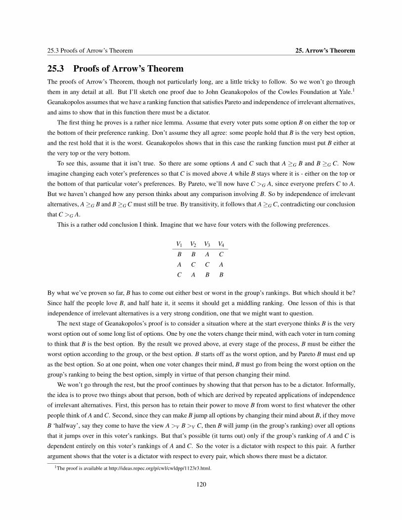
25.3 Proofs of Arrow’s Theorem 25. Arrow’s Theorem

25.3 Proofs of Arrow’s TheoremThe proofs of Arrow’s Theorem, though not particularly long, are a little tricky to follow. So we won’t go through

them in any detail at all. But I’ll sketch one proof due to John Geanakopolos of the Cowles Foundation at Yale.1

Geanakopolos assumes that we have a ranking function that satisfies Pareto and independence of irrelevant alternatives,

and aims to show that in this function there must be a dictator.

The first thing he proves is a rather nice lemma. Assume that every voter puts some option B on either the top or

the bottom of their preference ranking. Don’t assume they all agree: some people hold that B is the very best option,

and the rest hold that it is the worst. Geanakopolos shows that in this case the ranking function must put B either at

the very top or the very bottom.

To see this, assume that it isn’t true. So there are some options A and C such that A ≥G B and B ≥G C. Now

imagine changing each voter’s preferences so that C is moved above A while B stays where it is - either on the top or

the bottom of that particular voter’s preferences. By Pareto, we’ll now have C >G A, since everyone prefers C to A.

But we haven’t changed how any person thinks about any comparison involving B. So by independence of irrelevant

alternatives, A≥G B and B≥G C must still be true. By transitivity, it follows that A≥G C, contradicting our conclusion

that C >G A.

This is a rather odd conclusion I think. Imagine that we have four voters with the following preferences.

V1 V2 V3 V4

B B A C

A C C A

C A B B

By what we’ve proven so far, B has to come out either best or worst in the group’s rankings. But which should it be?

Since half the people love B, and half hate it, it seems it should get a middling ranking. One lesson of this is that

independence of irrelevant alternatives is a very strong condition, one that we might want to question.

The next stage of Geanakopolos’s proof is to consider a situation where at the start everyone thinks B is the very

worst option out of some long list of options. One by one the voters change their mind, with each voter in turn coming

to think that B is the best option. By the result we proved above, at every stage of the process, B must be either the

worst option according to the group, or the best option. B starts off as the worst option, and by Pareto B must end up

as the best option. So at one point, when one voter changes their mind, B must go from being the worst option on the

group’s ranking to being the best option, simply in virtue of that person changing their mind.

We won’t go through the rest, but the proof continues by showing that that person has to be a dictator. Informally,

the idea is to prove two things about that person, both of which are derived by repeated applications of independence

of irrelevant alternatives. First, this person has to retain their power to move B from worst to first whatever the other

people think of A and C. Second, since they can make B jump all options by changing their mind about B, if they move

B ‘halfway’, say they come to have the view A >V B >V C, then B will jump (in the group’s ranking) over all options

that it jumps over in this voter’s rankings. But that’s possible (it turns out) only if the group’s ranking of A and C is

dependent entirely on this voter’s rankings of A and C. So the voter is a dictator with respect to this pair. A further

argument shows that the voter is a dictator with respect to every pair, which shows there must be a dictator.1The proof is available at http://ideas.repec.org/p/cwl/cwldpp/1123r3.html.

120

Chapter 26 Voting SystemsThe Arrow Impossibility Theorem shows that we can’t have everything that we want in a voting system. In particular,

we can’t have a voting system that takes as inputs the preferences of each voter, and outputs a preference ordering of

the group that satisfies these three constraints.

1. Unanimity: If everyone prefers A to B, then the group prefers A to B.

2. Independence of Irrelevant Alternatives: If nobody changes their mind about the relative ordering of A and

B, then the group can’t change its mind about the relative ordering of A and B.

3. No Dictators: For each voter, it is possible that the group’s ranking will be different to their ranking

Any voting system either won’t be a function in the sense that we’re interested in for Arrow’s Theorem, or will

violate some of those constraints. (Or both.) But still there could be better or worse voting systems. Indeed, there are

many voting systems in use around the world, and serious debate about which is best. In these notes we’ll look at the

pros and cons of a few different voting systems.

The discussion here will be restricted in two respects. First, we’re only interested in systems for making political

decisions, indeed, in systems for electing representatives to political positions. We’re not interested in, for instance,

the systems that a group of friends might use to choose which movie to see, or that an academic department might

use to hire new faculty. Some of the constraints we’ll be looking at are characteristic of elections in particular, not of

choices in general.

Second, we’ll be looking only at elections to fill a single position. This is a fairly substantial constraint. Many

elections are to fill multiple positions. The way a lot of electoral systems work is that many candidates are elected at

once, with the number of representatives each party gets being (roughly) in proportion to the number of people who

vote for that party. This is how the parliament is elected in many countries around the world (including, for instance,

Mexico, Germany and Spain). Perhaps more importantly, it is basically the norm for new parliaments to have such kind

of multi-member constituencies. But the mathematical issues get a little complicated when we look at the mechanisms

for selecting multiple candidates, and we’ll restrict ourselves to looking at mechanisms for electing a single candidate.

26.1 Plurality votingBy far the most common method used in America, and throughout much of the rest of the world, is plurality voting.

Every voter selects one of the candidates, and the candidates with the most votes wins. As we’ve already noted, this is

called plurality, or first-past-the-post, voting.

Plurality voting clearly does not satisfy the independence of irrelevant alternatives condition. We can see this if we

imagine that the voting distribution starts off with the table on the left, and ends with the table on the right. (The three

candidates are A, B and C, with the numbers at the top of each column representing the percentage of voters who have

the preference ordering listed below it.)

121

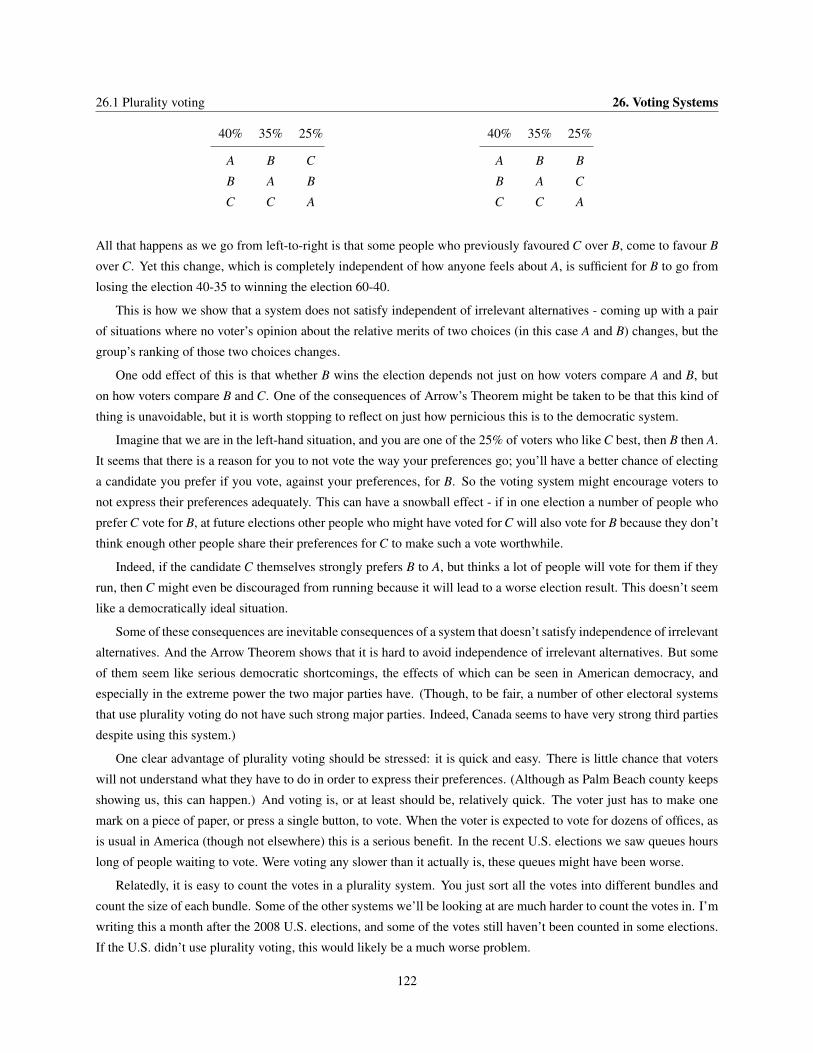
26.1 Plurality voting 26. Voting Systems

40% 35% 25% 40% 35% 25%

A B C A B B

B A B B A C

C C A C C A

All that happens as we go from left-to-right is that some people who previously favoured C over B, come to favour B

over C. Yet this change, which is completely independent of how anyone feels about A, is sufficient for B to go from

losing the election 40-35 to winning the election 60-40.

This is how we show that a system does not satisfy independent of irrelevant alternatives - coming up with a pair

of situations where no voter’s opinion about the relative merits of two choices (in this case A and B) changes, but the

group’s ranking of those two choices changes.

One odd effect of this is that whether B wins the election depends not just on how voters compare A and B, but

on how voters compare B and C. One of the consequences of Arrow’s Theorem might be taken to be that this kind of

thing is unavoidable, but it is worth stopping to reflect on just how pernicious this is to the democratic system.

Imagine that we are in the left-hand situation, and you are one of the 25% of voters who like C best, then B then A.

It seems that there is a reason for you to not vote the way your preferences go; you’ll have a better chance of electing

a candidate you prefer if you vote, against your preferences, for B. So the voting system might encourage voters to

not express their preferences adequately. This can have a snowball effect - if in one election a number of people who

prefer C vote for B, at future elections other people who might have voted for C will also vote for B because they don’t

think enough other people share their preferences for C to make such a vote worthwhile.

Indeed, if the candidate C themselves strongly prefers B to A, but thinks a lot of people will vote for them if they

run, then C might even be discouraged from running because it will lead to a worse election result. This doesn’t seem

like a democratically ideal situation.

Some of these consequences are inevitable consequences of a system that doesn’t satisfy independence of irrelevant

alternatives. And the Arrow Theorem shows that it is hard to avoid independence of irrelevant alternatives. But some

of them seem like serious democratic shortcomings, the effects of which can be seen in American democracy, and

especially in the extreme power the two major parties have. (Though, to be fair, a number of other electoral systems

that use plurality voting do not have such strong major parties. Indeed, Canada seems to have very strong third parties

despite using this system.)

One clear advantage of plurality voting should be stressed: it is quick and easy. There is little chance that voters

will not understand what they have to do in order to express their preferences. (Although as Palm Beach county keeps

showing us, this can happen.) And voting is, or at least should be, relatively quick. The voter just has to make one

mark on a piece of paper, or press a single button, to vote. When the voter is expected to vote for dozens of offices, as

is usual in America (though not elsewhere) this is a serious benefit. In the recent U.S. elections we saw queues hours

long of people waiting to vote. Were voting any slower than it actually is, these queues might have been worse.

Relatedly, it is easy to count the votes in a plurality system. You just sort all the votes into different bundles and

count the size of each bundle. Some of the other systems we’ll be looking at are much harder to count the votes in. I’m

writing this a month after the 2008 U.S. elections, and some of the votes still haven’t been counted in some elections.

If the U.S. didn’t use plurality voting, this would likely be a much worse problem.

122

26. Voting Systems 26.2 Runoff Voting

26.2 Runoff VotingOne solution to some of the problems with plurality voting is runoff voting, which is used in parts of America (notably

Georgia and Louisiana) and is very common throughout Europe and South America. The idea is that there are, in

general, two elections. At the first election, if one candidate has majority support, then they win. But otherwise the

top two candidates go into a runoff. In the runoff, voters get to vote for one of those two candidates, and the candidate

with the most votes wins.

This doesn’t entirely deal with the problem of a spoiler candidate having an outsized effect on the election, but it

makes such cases a little harder to produce. For instance, imagine that there are four candidates, and the arrangement

of votes is as follows.

35% 30% 20% 15%

A B C D

B D D C

C C B B

D A A A

In a plurality election, A will win with only 35% of the vote.1 In a runoff election, the runoff will be between A and

B, and presumably B will win, since 65% of the voters prefer B to A. But look what happens if D drops out of the

election, or all of D’s supporters decide to vote more strategically.

35% 30% 20% 15%

A B C C

B C B B

C A A A

Now the runoff is between C and A, and C will win. D being a candidate means that the candidate most like D, namely

C, loses a race they could have won.

In one respect this is much like what happens with plurality voting. On the other hand, it is somewhat harder to

find real life cases that show this pattern of votes. That’s in part because it is hard to find cases where there are (a)

four serious candidates, and (b) the third and fourth candidates are so close ideologically that they eat into each other’s

votes and (c) the top two candidates are so close that these third and fourth candidates combined could leapfrog over

each of them. Theoretically, the problem about spoiler candidates might look as severe, but it is much less of a problem

in practice.

The downside of runoff voting of course is that it requires people to go and vote twice. This can be a major

imposition on the time and energy of the voters. More seriously from a democratic perspective, it can lead to an

unrepresentative electorate. In American runoff elections, the runoff typically has a much lower turnout than the

initial election, so the election comes down to the true party loyalists. In Europe, the first round often has a very low

turnout, which has led on occasion to fringe candidates with a small but loyal supporter base making the final round.

1This isn’t actually that unusual in the overall scope of American elections. John McCain won several crucial Republican primary elections,

especially in Florida and Missouri, with under 35% of the vote. Without those wins, the Republican primary contest would have been much closer.

123

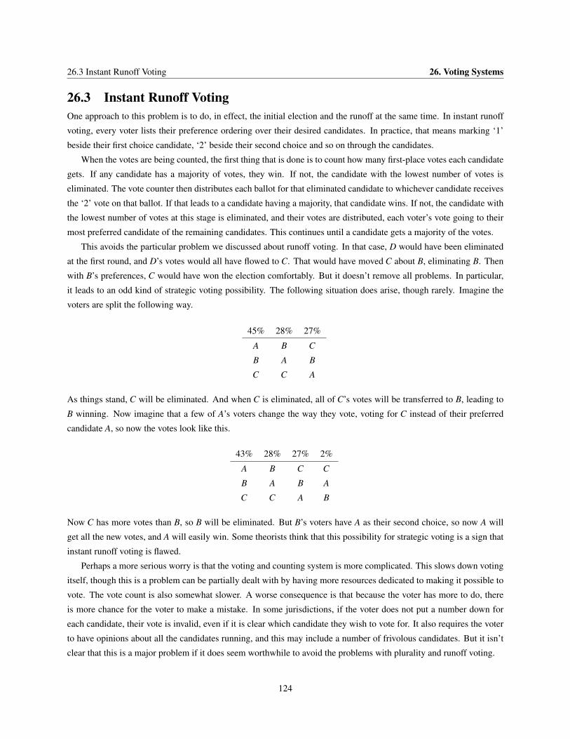
26.3 Instant Runoff Voting 26. Voting Systems

26.3 Instant Runoff VotingOne approach to this problem is to do, in effect, the initial election and the runoff at the same time. In instant runoff

voting, every voter lists their preference ordering over their desired candidates. In practice, that means marking ‘1’

beside their first choice candidate, ‘2’ beside their second choice and so on through the candidates.

When the votes are being counted, the first thing that is done is to count how many first-place votes each candidate

gets. If any candidate has a majority of votes, they win. If not, the candidate with the lowest number of votes is

eliminated. The vote counter then distributes each ballot for that eliminated candidate to whichever candidate receives

the ‘2’ vote on that ballot. If that leads to a candidate having a majority, that candidate wins. If not, the candidate with

the lowest number of votes at this stage is eliminated, and their votes are distributed, each voter’s vote going to their

most preferred candidate of the remaining candidates. This continues until a candidate gets a majority of the votes.

This avoids the particular problem we discussed about runoff voting. In that case, D would have been eliminated

at the first round, and D’s votes would all have flowed to C. That would have moved C about B, eliminating B. Then

with B’s preferences, C would have won the election comfortably. But it doesn’t remove all problems. In particular,

it leads to an odd kind of strategic voting possibility. The following situation does arise, though rarely. Imagine the

voters are split the following way.

45% 28% 27%

A B C

B A B

C C A

As things stand, C will be eliminated. And when C is eliminated, all of C’s votes will be transferred to B, leading to

B winning. Now imagine that a few of A’s voters change the way they vote, voting for C instead of their preferred

candidate A, so now the votes look like this.

43% 28% 27% 2%

A B C C

B A B A

C C A B

Now C has more votes than B, so B will be eliminated. But B’s voters have A as their second choice, so now A will

get all the new votes, and A will easily win. Some theorists think that this possibility for strategic voting is a sign that

instant runoff voting is flawed.

Perhaps a more serious worry is that the voting and counting system is more complicated. This slows down voting

itself, though this is a problem can be partially dealt with by having more resources dedicated to making it possible to

vote. The vote count is also somewhat slower. A worse consequence is that because the voter has more to do, there

is more chance for the voter to make a mistake. In some jurisdictions, if the voter does not put a number down for

each candidate, their vote is invalid, even if it is clear which candidate they wish to vote for. It also requires the voter

to have opinions about all the candidates running, and this may include a number of frivolous candidates. But it isn’t

clear that this is a major problem if it does seem worthwhile to avoid the problems with plurality and runoff voting.

124

Chapter 27 More Voting SystemsIn the previous chapter we looked at a number of voting systems that are in widespread use in various democracies.

Here we look at three voting systems that are not used for mass elections anywhere around the world, though all of

them have been used in various purposes for combining the views of groups. (For instance, they have been used for

elections in small groups.)

27.1 Borda CountIn a Borda Count election, each voter ranks each of the candidates, as in Instant Runoff Voting. Each candidate then

receives n points for each first place vote they receive (where n is the number of candidates), n− 1 points for each

second place vote, and so on through the last place candidate getting 1 point. The candidate with the most points wins.

One nice advantage of the Borda Count is that it eliminates the chance for the kind of strategic voting that exists in

Instant Runoff Voting, or for that matter any kind of Runoff Voting. It can never make it more likely that A will win by

someone changing their vote away from A. Indeed, this could only lead to A having fewer votes. This certainly seems

to be reasonable.

Another advantage is that many preferences beyond first place votes count. A candidate who is every single voter’s

second best choice will not do very well under any voting system that gives a special weight to first preferences. But

such a candidate may well be in a certain sense the best representative of the whole community.

And a third advantage is that the Borda Count includes a rough approximation of voter’s strength of preference. If

one voter ranks A a little above B, and another votes B many places above A, that’s arguably a sign that B is a better

representative of the two of them than A. Although only one of the two prefers B, one voter will be a little disappointed

that B wins, while the other would be very disappointed if B lost.

These are not trivial advantages. But there are also many disadvantages which explain why no major electoral

system has adopted Borda Count voting yet, despite its strong support from some theorists.

First, Borda Count is particularly complicated to implement. It is just as difficult for the voter to as in Instant

Runoff Voting; in each case they have to express a complete preference ordering. But it is much harder to count,

because the vote counter has to detect quite a bit of information from each ballot. Getting this information from

millions of ballots is not a trivial exercise.

Second, Borda Count has a serious problem with ‘clone candidates’. In plurality voting, a candidate suffers if

there is another candidate much like them on the ballot. In Borda Count, a candidate can seriously gain if such a

candidate is added. Consider the following situation. In a certain electorate, of say 100,000 voters, 60% of the voters

are Republicans, and 40% are Democrats. But there is only one Republican, call them R, on the ballot, and there are

2 Democrats, D1 and D2 on the ballot. Moreover, D2 is clearly a worse candidate than D1, but the Democrats still

prefer the Democrat to the Republican. Since the district is overwhelmingly Republican, intuitively the Republican

should win. But let’s work through what happens if 60,000 Republicans vote for R, then D1, then D2, and the 40,000

125

27.2 Approval Voting 27. More Voting Systems

Democrats vote D1 then D2 then R. In that case, R will get 60,000× 3 + 40,000× 1 = 220,000 points, D1 will get

60,000×2+40,000×3 = 240,000 points, and D2 will get 60,000×1 +40,000×2 = 140,000 points, and D1 will

win. Having a ‘clone’ on the ticket was enough to push D1 over the top.

On the one hand, this may look a lot like the mirror image of the ‘spoiler’ problem for plurality voting. But in

another respect it is much worse. It is hard to get someone who is a lot ideologically like your opponent to run in order

to improve your electoral chances. It is much easier to convince someone who already wants you to win to add their

name to the ballot in order to improve your chances. In practice, this would either lead to an arms race between the

two parties, each trying to get the most names onto the ballot, or very restrictive (and hence undemocratic) rules about

who was even allowed to be on the ballot, or, most likely, both.

The third problem comes from thinking through the previous problem from the point of view of a Republican

voter. If the Republican voters realise what is up, they might vote tactically for D2 over D1, putting R back on top. In

a case where the electorate is as partisan as in this case, this might just work. But this means that Borda Count is just

as susceptible to tactical voting as other systems; it is just that the tactical voting often occurs downticket. (There are

more complicated problems, that we won’t work through, about what happens if the voters mistakenly judge what is

likely to happen in the election, and tactical voting backfires.)

Finally, it’s worth thinking about whether the supposed major virtue of Borda Count, the fact that it considers all

preferences and not just first choices, is a real gain. The core idea behind Borda Count is that all preferences should

count equally. So the difference between first place and second place in a voter’s affections counts just as much as

the difference between third and fourth. But for many elections, this isn’t how the voters themselves feel. I suspect

many people reading this have strong feelings about who was the best candidate in the past Presidential election. I

suspect very few people had strong feelings about who was the third best versus fourth best candidate. This is hardly

a coincidence; people identify with a party that is their first choice. They say, “I’m a Democrat” or “I’m a Green” or

“I’m a Republican”. They don’t identify with their third versus fourth preference. Perhaps voting systems that give

primary weight to first place preferences are genuinely reflecting the desires of the voters.

27.2 Approval VotingIn plurality voting, every voter gets to vote for one candidate, and the candidate with the most votes wins. Approval

voting is similar, except that each voter is allowed to vote for as many candidates as they like. The votes are then

added up, and the candidate with the most votes wins. Of course, the voter has an interest in not voting for too many

candidates. If they vote for all of the candidates, this won’t advantage any candidate; they may as well have voted for

no candidates at all.

The voters who are best served by approval voting, at least compared to plurality voting, are those voters who wish

to vote for a non-major candidate, but who also have a preference between the two major candidates. Under approval

voting, they can vote for the minor candidate that they most favour, and also vote for the the major candidate who

they hope will win. Of course, runoff voting (and Instant Runoff Voting) also allow these voters to express a similar

preference. Indeed, the runoff systems allow the voters to express not only two preferences, but express the order in

which they hold those preferences. Under approval voting, the voter only gets to vote for more than one candidate,

they don’t get to express any ranking of those candidates.

But arguably approval voting is easier on the voter. The voter can use a ballot that looks just like the ballot used

in plurality voting. And they don’t have to learn about preference flows, or Borda Counts, to understand what is going

126

27. More Voting Systems 27.3 Range Voting

on in the voting. Currently there are many voters who vote for, or at least appear to try to vote for, multiple candidates.

This is presumably inadvertent, but approval voting would let these votes be counted, which would refranchise a

number of voters. Approval voting has never been used as a mass electoral tool, so it is hard to know how quick it

would be to count, but presumably it would not be incredibly difficult.

One striking thing about approval voting is that it is not a function from voter preferences to group preferences.

Hence it is not subject to the Arrow Impossibility Theorem. It isn’t such a function because the voters have to not

only rank the candidates, they have to decide where on their ranking they will ‘draw the line’ between candidates that

they will vote for, and candidates that they will not vote for. Consider the following two sets of voters. In each case

candidates are listed from first preference to last preference, with stars indicating which candidates the voters vote for.

40% 35% 25% 40% 35% 25%

∗A ∗B ∗C ∗A ∗B ∗CB A B B A ∗BC C A C C A

In the election on the left-hand-side, no voter takes advantage of approval voting to vote for more than one candidate.

So A wins with 40% of the vote. In the election on the right-hand-side, no one’s preferences change. But the 25% who

prefer C also decide to vote for B. So now B has 60% of the voters voting for them, as compared to 40% for A and

25% for C, so B wins.

This means that the voting system is not a function from voter preferences to group preferences. If it were a

function, fixing the group preferences would fix who wins. But in this case, without a single voter changing their

preference ordering of the candidates, a different candidate won. Since the Arrow Impossibility Theorem only applies

to functions from voter preferences to group preferences, it does not apply to Approval Voting.

27.3 Range VotingIn Range Voting, every voter gives each candidate a score. Let’s say that score is from 0 to 10. The name ‘Range’

comes from the range of options the voter has. In the vote count, the score that each candidate receives from each

voter is added up, and the candidate with the most points wins.

In principle, this is a way for voters to express very detailed opinions about each of the candidates. They don’t

merely rank the candidates, they measure how much better each candidate is than all the other candidates. And this

information is then used to form an overall ranking of the various candidates.

In practice, it isn’t so clear this would be effective. Imagine that a voter V thinks that candidate A would be

reasonably good, and candidate B would be merely OK, and that no other candidates have a serious chance of winning.

If V was genuinely expressing their opinions, they might think that A deserves an 8 out of 10, and B deserves a 5 out

of 10. But V wants A to win, since V thinks A is the better candidate. And V knows that what will make the biggest

improvement in A’s chances is if they score A a 10 out of 10, and B a 0 out of 10. That will give A a 10 point advantage,

whereas they may only get a 3 point advantage if the voter voted sincerely.

It isn’t unusual for a voter to find themselves in V ’s position. So we might suspect that although Range Voting will

give the voters quite a lot of flexibility, and give them the chance to express detailed opinions, it isn’t clear how often

it would be in a voter’s interests to use these options.

127

27.4 Exercises 27. More Voting Systems

And Range Voting is quite complex, both from the perspective of the voter and of the vote counter. There is a lot of

information to be gleaned from each ballot in Range Voting. This means the voter has to go to a lot of work to fill out

the ballot, and the vote counter has to do a lot of work to process all that information. This means that Range Voting

might be very slow, both in terms of voting and counting. And if voters have a tactical reason for not wanting to fill

in detailed ballots, this might mean it’s a lot of effort for not a lot of reward, and that we should stick to somewhat

simpler vote counting methods.

27.4 ExercisesFor each of the following voting systems, say (a) whether they are functions from expressed preferences of voters to a

preference ordering by the group, and, if so, (b) which of the Arrow constraints (unanimity, no dictators, independence

of irrelevant alternatives) they fail to satisfy.

1. Runoff Voting

2. Instant Runoff Voting

3. Borda Count

4. Range Voting

For each case where you say the voting system is not a function, or say that a constraint is not satisfied, you should

give a pair of examples (like the pairs on pages 122 and 127) to demonstrate this.

128

decision theory. Note - Brian Weatherson

Documents

Transcript of decision theory. Note - Brian Weatherson