Decision Support System for Adaptive Water Supply...

ta, andnt andof ahe DSSear andctives

tions. The

Decision Support System for Adaptive WaterSupply Management

Kirk S. Westphal, M.ASCE1; Richard M. Vogel, M.ASCE2; Paul Kirshen, M.ASCE3;and Steven C. Chapra, M.ASCE4

Abstract: Recent advances in computer technology and water resource modeling, availability of real-time hydroclimatic daimprovements in our ability to develop user-friendly graphical model interfaces have led to significant growth in the developmeapplication of decision support systems~DSSs! for water resource systems. This study provides an example of the developmentreal-time DSS for adaptive management of the reservoir system that provides drinking water to the Boston metropolitan region. Tuses a systems framework to link watershed models, reservoir hydraulic models, and a reservoir water quality model with linnonlinear optimization algorithms. The DSS offers the ability to optimize daily and weekly reservoir operations toward four objebased on short-term climate forecasts:~1! maximum water quality,~2! ideal flood control levels,~3! optimum reservoir balancing, and~4!maximum hydropower revenues. Case studies document the value of the DSS as an enhancement of current rule curve operastudy shows that simple tools, in this case, familiar spreadsheet software, can be used to improve system efficiencies.

DOI: 10.1061/~ASCE!0733-9496~2003!129:3~165!

CE Database subject headings: Decision support systems; Water supply; Boston; Massachusetts; Water management.

ont,stc-gdslltesoing

lie.is,nory

hlycli-g

tialand

hy-t a

nu-ndi-

od,. Itof-are

el-of

edual-e

h-ond-en-ter

lityear

op-or-

eets

e-

p-

r-

d

-

onsbygs-his

-

IntroductionFor many water supply systems, reservoir operations are basedheuristic approaches including rule curves, operator judgmeand other qualitative information. While often reliable and coeffective, such techniques often pertain only to individual objetives, and usually do not offer guidance for adaptively fine tunina system as real-time conditions change over short time perioThis study is an effort to quantify, organize, and process asources of information necessary to adaptively manage the wasupply system that services the Boston Metropolitan regionthat long-term plans can be adapted on a weekly basis to changconditions and time-varying objectives.

The Massachusetts Water Resources Authority~MWRA! oper-ates a two-reservoir system in central Massachusetts that suppdrinking and industrial water to the Boston Metropolitan regionHistorically, operational decisions were made on a monthly baswith the assistance of rule curves, and the system has beereliable source of water for many decades. Despite satisfact

1Water Resources Engineer, CDM, One Cambridge Place, 50 Hamshire St., Cambridge, MA 02139. E-mail: [email protected]

2Professor, Tufts Univ., Dept. of Civil and Environmental Engineeing, Medford, MA 02155. E-mail: [email protected]

3Research Associate Professor, Tufts Univ., Dept. of Civil anEnvironmental Engineering, Medford, MA 02155. E-mail:[email protected]

4Professor and Berger Chair, Tufts Univ., Dept. of Civil and Environmental Engineering, Medford, MA 02155.E-mail: [email protected]

Note. Discussion open until October 1, 2003. Separate discussimust be submitted for individual papers. To extend the closing dateone month, a written request must be filed with the ASCE ManaginEditor. The manuscript for this paper was submitted for review and posible publication on November 7, 2001; approved on June 17, 2002. Tpaper is part of theJournal of Water Resources Planning and Manage-ment, Vol. 129, No. 3, May 1, 2003. ©ASCE, ISSN 0733-9496/2003/3165–177/$18.00.

JOURNAL OF WATER RESOURC

n

.

r

s

a

yield, however, MWRA managers recognized that the monttimescale for operational decisions was not compatible withmate variability within each month in New England. Promotinthe highest possible water quality and preparing for potenfloods require adaptive management of the system as climatichydrologic events occur. With real-time climate forecasts anddrologic data readily available, MWRA managers decided thareal-time DSS could help improve operations with respect tomerous objectives based on expected hydroclimatological cotions.

A real-time DSS is developed for a seven-day planning periand its output is based on input of current climate forecastsallows planners to maximize or minimize, as applicable, anyfour objectives individually or in hierarchical multiobjective formulations, depending on circumstances. The four objectivesthe minimization of total organic carbon~TOC! in the down-stream reservoir, the minimization of deviations from targetevations, balancing the two reservoirs, and the maximizationrevenues from three hydropower facilities. It is normally assumthat the water supply system satisfies demand so that water qity and flood control are normally the primary objectives. ThMWRA has historically operated the hydropower facilities witout economic intent; hence power revenues are always a secary objective. Nevertheless, we document that hydropower befits may be increased while still achieving the primary waquality and/or flood control objectives.

The DSS combines hydrologic, hydraulic, and water quamodels into a system optimization model that uses both linprograms~LPs! and nonlinear programs~NLPs!. Since prospec-tive users of the DSS include engineers, managers, and fielderators, practicality and transportability were of paramount imptance. Hence, commonly usedWindows-based software wasselected. Model components were developed on spreadshusing MicrosoftExcelandVisual Basic for Applications~VBA !.Visual Basic for Applications provided a mechanism for the d

ES PLANNING AND MANAGEMENT © ASCE / MAY/JUNE 2003 / 165

aan

,

6

i

ma

ymy

ue-ra-

iver.owon-

from

.174

tghly

ge ofticutes-

n inift

ns-theire-

t into

elieseedsthed to

es-ThearebinBe-

rmitsthe

ur-ime.the

de-

ly

velopment of a functional graphical user interface as well asmechanism for model integration, data transfer, and numericsolutions. Optimization algorithms include those available withian enhanced version of the standardExcel SOLVER. The resultingDSS is a singleExcel workbook that can be easily understoodapplied, and modified by engineers and system operators.

System Description and Management Options

The water supply system supplies 46 communities~roughly 2.5million people! in eastern Massachusetts with an average of 0.9million m3 ~MCM! of water per day. It consists of two reservoirsin series as depicted in Figs. 1 and 2. The Quabbin Reservolocated 130 km west of Boston, has a 490 km2 watershed, and canstore up to 1,560 MCM of water~966 MCM active storage!. TheWachusett Reservoir, 40 km closer to Boston, has a 277 km2

watershed, and can store up to 246 MCM of water~36.7 MCMactive storage!. The Wachusett Reservoir also receives water frothe Quabbin Reservoir via the Quabbin Aqueduct, and servesthe final retention basin for the water before it is chemicalltreated. In between the two basins flows the Ware River. FroOctober 15 through June 14, water in excess of 0.32 MCM/da

Fig. 1. Massachusetts Water Resources Authority water suppsystem

166 / JOURNAL OF WATER RESOURCES PLANNING AND MANAGEMEN

l

r,

s

can be diverted to the Quabbin Reservoir via the Quabbin Aqduct. However, river diversions significantly restrict other opetional activity, and can cause operational conflicts.

The westernmost system component is the Connecticut RThe river does not supply the MWRA system with water, but flin the river, as measured at the USGS gauging station in Mtague, Mass., governs minimum daily downstream releasesthe Quabbin Reservoir to the Swift River~which eventually flowsinto the Connecticut River and is lost from the system!. The mini-mum daily release rate is 0.076 MCM, but this increases to 0MCM when Connecticut River flow drops below 139 m3/s, and to0.269 MCM when flow drops below 132 m3/s. Considering thathe estimated value of safe yield from the entire system is rou1.14 MCM/day ~Vogel and Hellstrom 1988!, these minimumdownstream release rates represent a significant percentaavailable water. The DSS predicts streamflow in the ConnecRiver in order to include this important constraint on weekly rervoir operations.

The system includes three hydropower stations, as showFig. 2, with a total capacity of 8 MW. Water released to the SwRiver flows through the turbines at Winsor Station. Water traferred from Quabbin to Wachusett can pass either throughturbines at Oakdale or through bypass pipes when flow requments exceed turbine ratings. Water released from Wachusetthe Cosgrove Tunnel passes through the Cosgrove turbines.

The Quabbin Aqueduct connects the two reservoirs, and ron gravity to accommodate the three separate operational ndepicted in Fig. 3. First, it can be used to divert water fromWare River into the Quabbin Reservoir. It can also be usetransfer water from the Quabbin Reservoir to the Wachusett Rervoir, through either a hydropower station or a bypass pipe.bypass valves are nonregulating valves, and when theyopened, the flow is governed only by the head in the QuabReservoir and the physical characteristics of the aqueduct.cause the turbines are flow limited, the bypass mechanism petransfer rates nearly twice as high as are possible throughturbines. Operationally, the single aqueduct fulfills three pposes, but only one operational mode is possible at a given t

Figs. 2 and 3 illustrate the management alternatives forsystem. For every 7-day planning period, the following dailycisions are needed: how much water, if any,~1! to divert from the

Fig. 2. Schematic of Massachusetts Water Resources Authority water supply system

T © ASCE / MAY/JUNE 2003

Fig. 3. Schematic of aqueduct transfers and diversions

a

tecon

itsuleelsndhe

rauto-or

ingouriodachns

e ofis-um

ongll-hs

iza-

t isam.Aor

ndtedere-is

er-

ayrag-of--inty

al.el

lish

tout

Ware River, ~2! to transfer from Quabbin to Wachusett viOakdale Station,~3! to transfer via the bypass pipes,~4! to releasefrom Quabbin downstream, and~5! to release from Wachusetdownstream. It is the purpose of this DSS to enable such dsions to be made in an objective, adaptive, and optimal fashi

Program Structure and Interface

Although the entire DSS is contained within a single PC file,components were designed in a modular framework. The modare interconnected as illustrated in Fig. 4. The hydrologic modare run as soon as the user inputs climate forecasts, initial cotions, and the constraints that may vary from week to week. Toutput of the watershed models is then transferred to the hydlic and optimization modules. The hydraulic models adjust aumatically during optimization, and continually update the LPNLP with values of system variables and constraints.

Fig. 4. Block diagram of decision support system


i-.

s

i-

-

Output is transferred to the user interface three times durthe running of the DSS. First, as soon as the hydrology of the fbasins is simulated, the predicted flows for the planning perare presented along with 12-month historic hydrographs of ebasin. This output allows the users to evaluate runoff predictioin the context of recent trends, and to evaluate the performancthe rainfall-runoff models. The second set of output data is dplayed once the optimization module has determined an optimoperating schedule for the chosen objective~s!. The 7-day sched-ule of daily releases, transfers, and diversions is displayed alwith predictions of surface levels, 7-day basin yield, total spiage, and hydropower revenues. Finally, water quality grapbased on the optimized schedule are provided after the optimtion is complete.

Users interact with the DSS through a control screen thastructured as a flowchart for easy navigation through the progrEach ‘‘button’’ on the control screen, when clicked, calls a VBsubroutine that either displays a dialogue box for data entrytriggers the various modules within the DSS, including LPs aNLPs. From this control screen, optimization can be repeawith different objectives or combinations of objectives. Also, thcontrol screen offers options to evaluate water quality and focast sensitivity. In this way, all decision-support informationaccessible from a single control screen. See Westphal~2001! forthe graphics of all interface screens.

Modeling Techniques

Hydrologic Modeling

The hydrologic models predict watershed runoff into both resvoirs and streamflow in the Ware and Connecticut Rivers~systemconstraints!. Streamflow predictions are based on real-time 7-dforecasts of precipitation and temperature ranges. Weekly aveing is used since the operating objectives focus only on end-week conditions~not on the day-to-day variability of system conditions!, and since this technique avoids unnecessary uncertain daily hydrologic responses of the large watersheds.~Opera-tional flows are accounted for on adaily basis to allow aqueductflow in two directions during any given week, yet only the totweekly flows are important in computing the objective functions!The flow predictions are used in the reservoir optimization modto constrain the natural inflows to the system and to estabmandated constraints on diversions and releases.

Critical to the success of any real-time DSS is its abilityaccurately predict watershed runoff using a minimum of inp


Fig. 5. Weekly yield model performance

dn

-edcu

s-

rors

do

ns

dee-

,l.

e,

i-orors-

sey

tgeeel-ge

i-

ilyg

data~Loucks 1995!. Four independent watershed models areveloped to predict the watershed yield for the Quabbin aWachusett Reservoirs and flow in the Ware and Connecticut Rers. Reservoir yieldY is defined as

Yti5Qti1Pti2Eti1Gti (1)

where Q5streamflow; P5precipitation onto the reservoir surface; E5free-surface evaporation; andG5groundwater seepagfor planning periodt at site i. Streamflow, evaporation, angroundwater seepage are determined using independentlybrated models based on expected precipitation and temperat

Streamflow is predicted using a modified version of theabcdwater balance model introduced by Thomas~1981!. This modeluses four physically based parameters~a, b, c, andd! to computeinflows and outflows from two storage variables; near-surfacemoisture and groundwater~aquifer! storage, according to the following equations:

Available water: Wt5Pt1St21 (2)

Evapotranspiration opportunity:

Yt5FWt1b

2a2A@~Wt1b!/2a#22bWt /aG (3)

Soil moisture storage: St5Yt expS 2PEt

b D (4)

Groundwater storage: Gt5c~Wt2Yt!1Gt21

11d(5)

Actual evapotranspiration: Et5Yt2St (6)

Streamflow: Qt5@~12c!~Wt2Yt!1dGt# (7)

For each timestep, the model computesavailable water(Wt) asthe sum of previous soil moisture (St21) and current precipitation(Pt). Evapotranspiration opportunity(Yt) is defined as the watethat will eventually leave the basin through evapotranspiratiand is used to help define how much of the available watermains in the basin during each timestep. Potential evapotranration (PEt) is estimated using the Hargreaves method~Har-greaves and Samani 1982!; among all temperature-based methoof potential evapotranspiration, the Hargreaves method is theone recommended by Shuttleworth and Maidment~1993!. Theequations distribute available water between runoff, percolatiogroundwater, change in soil moisture storage, and evapotran

168 / JOURNAL OF WATER RESOURCES PLANNING AND MANAGEME

e-d

iv-

ali-re.

oil

n,e-pi-

snly

topi-

ration (Et). Groundwater storage (Gt) and soil moisture (St) aresimulated as separate storage reservoirs. Streamflow (Qt) is sim-ply the sum of baseflow and runoff, where baseflow is estimateas a linear function of groundwater storage. Modifications weradded to account for snow accumulation and melting, and threduction in evapotranspiration caused by subfreezing air temperatures. Theabcd model is an attractive watershed model forthis DSS because~1! its parameters are physically based~seeFernandez et al. 2000!, ~2! it is a parsimonious model having onlyfive parameters with the addition of the snowmelt modificationsthereby conforming to recommendations by Hornberger et a~1985!, Hooper et al.~1988!, Beven ~1989!, and Jakeman andHornberger~1993!, ~3! it requires only precipitation and tempera-ture as input,~4! it provides estimates of internal watershed statevariables including groundwater storage, soil moisture storagand actual evapotranspiration, and~5! it compares favorably withother commonly used water balance models~see Alley 1984;Vanderwiele et al. 1992!.

Ideally, free-surface evaporation would be estimated from ether pan evaporation data or the Penman-Montieth approach festimating potential evaporation. Since data are unavailable feither approach, the following temperature-based approach to etimating reservoir evaporation was employed:

SEti5ati PEtiAti (8)

whereSEti5free-surface evaporation for weekt and reservoiri;ati5calibrated coefficient;PEti5potential evapotranspirationcomputed using the Hargreaves method; andAti5reservoir sur-face area. The calibration parameters in Eq.~8! were obtained bycomparing regional regression equations developed by Fennesand Vogel~1996! for estimating monthly mean potential evapora-tion ~PE! from very limited data. Fennessey and Vogel show thatheir regression equations reproduce long-term monthly averavalues of PE based on the widely used but data-intensivPenman-Monteith approach. Finally, a seepage model was devoped for each reservoir based on modeled groundwater storalevels and time of year~Westphal 2001!. The models of eachhydrologic contributor are combined for each reservoir to estmate reservoir yield using Eq.~1!. The results shown in Fig. 5indicate that the reservoir yield models reproduce average dayield for 7-day periods with reasonable accuracy, explaininroughly 75–80% of the weekly variations in overall yield. Addi-

NT © ASCE / MAY/JUNE 2003

w

Table 1. Controlled Reservoir Releases

Release from Release to Medium Method of determining flo

Quabbin Swift River~min! Winsor Power Station Connecticut River modelSwift River ~extra! Winsor Power Station Optimization programSpringfield suburbs Chicopee Valley Aqueduct User input

Wachusett Nashua River~min! Fountain at Dam User inputNashua River~extra! ‘‘Waste Gates’’ Optimization program

Lancaster Mills Fountain at Dam User inputTown of Clinton Pipeline User input

Town of Leominster Pipeline User inputMetro West Towns Wachusett Aqueduct User input

Boston Metro Cosgrove Power Station, Cosgrove Tunnel User input

wm

t

ek

iomt

edelre

setivta

puiaba

ed

yd

.

r-y

al

ch

d

rte

s-a-yl-,, is

ofm

tionally, the Connecticut River model predicts the correct floregime 92% of the time, and the Ware River model exhibits silar accuracy.

Hydraulic Reservoir Models

Reservoir operations for each reservoir are modeled usingcontinuity equation

St5St211(j

Inflowj2(k

Outflowk (9)

whereSt5storage volume at the end of weekt. The inflows andoutflows to each reservoir can be disaggregated for any weperiod using

( Inflowsj5Drainage1Precipsurf

1(i 51

7

Transferi in1(i 51

7

Divi (10a)

( Outflowsk5Evaporation1Seepage17(n

RELn

1(i 51

7

Transferi out1Spill (10b)

where each value ofRELn represents one ofn possible controlleddaily releases from the reservoir, andi is a daily index.

The hydrologic terms are discussed in the previous sectTransfers occur in the Quabbin Aqueduct, and since the systeentirely gravity fed water can only be transferred from QuabbinWachusett~Figs. 2 and 3!. Regulated transfer flow can be passthrough turbines at the Oakdale hydropower station. Alternativflow in excess of the maximum turbine rating can be transferinto Wachusett by bypassing the turbines via nonregulating~full-flow! valves. In such cases, flow is determined not by valvetings but by the physical features of the aqueduct and relahead levels in the reservoirs. Diversions represent flow thadiverted from the Ware River into the Quabbin Reservoir, andexpressed by the daily decision variablesDivi . Controlled re-leases represent reservoir withdrawals for downstream flowMWRA water users. Release values are determined via user inresults of hydrologic modeling, or system optimization, as olined in Table 1. Spills from Quabbin are estimated from initelevation, and spills from Wachusett are estimated from massance estimates~assuming that all excess water in Wachusett cspill within one week!.

JOURNAL OF WATER RESOUR

i-

he

ly

n.is

o

y,d

t-eisre

orut,t-lal-n

Because only one aqueduct fulfills three purposes, only onoperational mode is possible at a given time, and the simulateaqueduct is limited to only one function per day. Eqs.~11a! and~11b! combine continuous and binary variables to define dailflow in the aqueduct with linear equations, based on physical anoperational limitations

Transferi5Qmin~CheckTrani !1Trani1Limitbypass~CheckBypi !(11a)

Divi5 f ~CheckDivi ,Constraints! (11b)

where Qmin5minimum rated turbine flow; Trani5transferthrough turbines in excess ofQmin on dayi ~continuously variablefrom zero to an upper bound!; and Limitbypass5hydraulic limitcomputed for the bypass circuit as a function of differential headCheckTrani , CheckBypi , andCheckDivi are all binary variablesthat are set equal to 1 if their corresponding function is detemined to be optimum, or 0 if not, and the sum of the three for andaily value ofi is constrained to 1.Trani is also constrained to 0if CheckTrani is 0. The upper bound ofTrani is estimated eachweek as a constant from historical records based on relative initihead levels, and the value ofLimitbypassis determined each weekas a constant using the energy equation and the Darcy-Weisbaequation with calibrated friction factors. The values ofDivi areoptimized, and vary from 0 to an upper limit computed fromhydrologic simulation and numerous hydraulic, operational, anlegislated constraints~presented later!. They are constrained to 0if CheckDivi is equal to 0. This technique converts nonlinearfunctions and discontinuities into a simple, mixed-integer lineaformat, by segmenting the equations into continuous and discreblocks: Transferi is either the sum of a discrete minimum valueand the continuous variableTrani , or it is equal to the discretevalue of the maximum bypass flow.

Other important hydraulic relationships are those between reervoir volume, surface elevation, and surface area. Surface elevtion is a measurable quantity, and is used by MWRA as a primarguide in operational decision making. Unfortunately, surface eevation is a nonlinear function of reservoir volume, and the DSSas designed, uses LPs for greatest efficiency. Storage, howevera linear function of inflows and outflows@Eqs. ~9!–~10b!#, andthis linearity permits fully linear simulation of the reservoir hy-draulics. User input and DSS output are expressed in termssurface elevation, since this is the familiar standard. The prograsimply converts elevation to volume prior to, and following, theoptimization algorithm. The MWRA has developed the followingregression relationships between volume and elevation (R2

.0.99):

CES PLANNING AND MANAGEMENT © ASCE / MAY/JUNE 2003 / 169

tra-

in--edontesor-

Cbledel
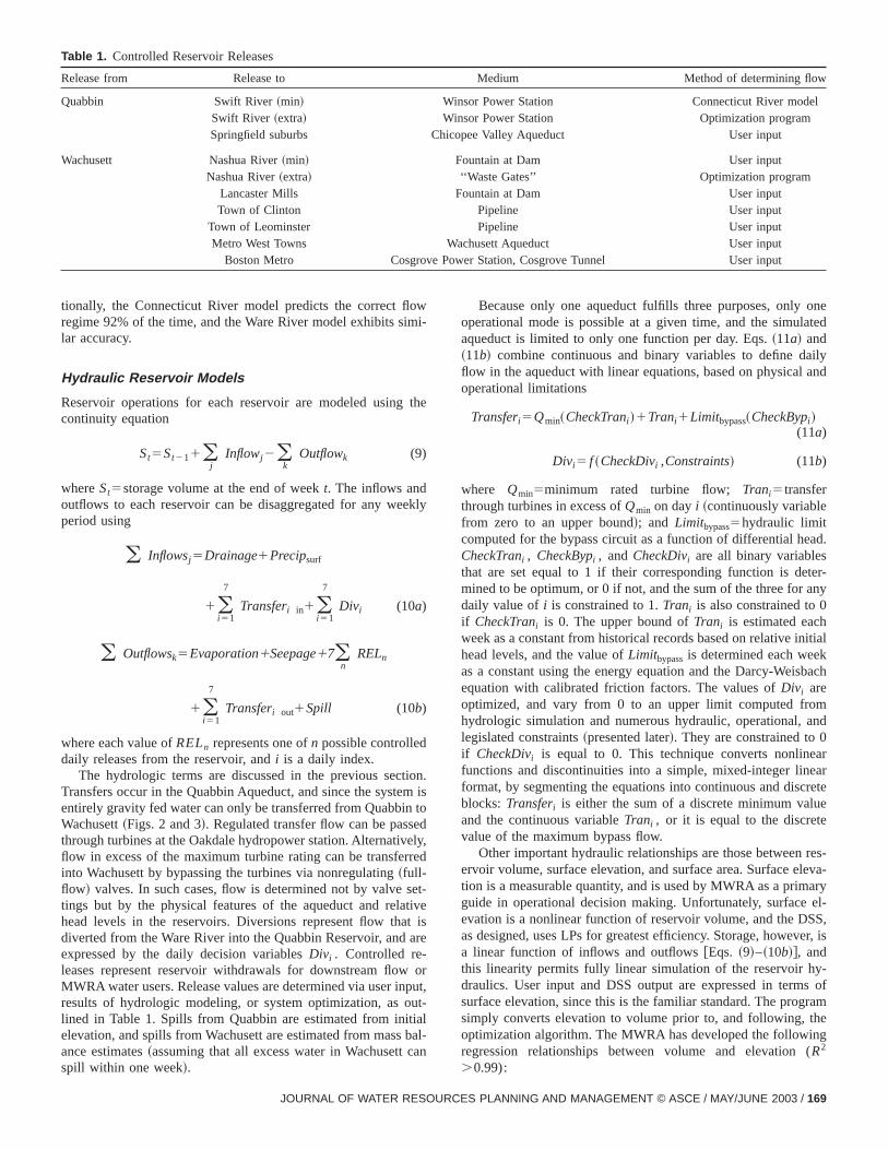
Fig. 6. Segmentation of Wachusett Reservoir in water quality mo
s

ac

a

ionpewch

esdgtot

cy

onizeoinaiswtoheinn

r,toeaing

ific.silyslers

theratee

ls,vea-ndncere

hisoni-res-

the

ewol of

etto-

hem-rend

re-d-oirfor4

et-sonthe


h

-

r--

-

al

-

dr.l

-

-

-

much easier to obtain. The MWRA uses the absorbance of ulviolet light at a wavelength of 254 nm~UV-254 absorbance! toindicate required chlorination levels and expected levels of disfection byproducts~DBPs!. From a modeling perspective, predicting rates of light absorbance is difficult, but TOC can be modelby considering the advection, diffusion, settling, and productiof organic material throughout the reservoir. Our model simulaTOC and the results are correlated to levels of UV-254 absbance using

UV-25450.4456~TOC!20.5918 (14)

where UV-254 is in units of absorbance in a 10 cm cell, and TOis expressed in mg/L. This correlation is based on 29 availadata points, and the model exhibits anR2 value of 0.73. It isheavily influenced by four outliers~without which theR2 valueincreases to 0.85!. MacCraith et al.~1993! and MatscheandStumwohrer ~1996! confirm that UV-254 and TOC are well cor-related, although the relationships are known to be site specAs more data become available, the correlation model can eabe refined. As it is, the numerical water quality model provideMWRA with an estimate of the effects of any optimized scheduon the TOC in the reservoir, and the correlation relationship offea reasonable estimate of the resulting level of UV-254 neartreatment plant intake. The authors are developing a sepamanuscript that will describe the water quality model and thcorrelation between UV-254 and TOC in greater detail.

While data pertaining to TOC concentrations, reservoir leveand inflows were readily available, other data that would habeen useful in the development and calibration of a fully mechnistic model were not. Algal biomass, phosphorus, nitrogen, atemperature data were either sparse or unavailable, and hestratification and the occurrence of spring algae blooms webased on historical trends. In a real-time model, however, tposes no problem, since users can use available real-time mtoring data to answer yes/no questions about the state of theervoir each week~such as, ‘‘Is the reservoir fully stratified?’’!.Their answers are converted to binary variables that simulatestate of the reservoir mathematically.

Stratification is particularly important in this model, since ththermal structure of the stored water affects the flow paths of tmajor source rivers and the water transferred from Quabbin, alwhich enter at the western end of the reservoir~see Fig. 6!. Thereservoir is typically stratified from mid-May through mid-October. Quabbin water is usually much colder than Wachuswater, and we might expect that it would plunge downward tward the hypolimnion. However, when Thomas Basin~section 1in Fig. 6! receives water from both the aqueduct and rivers, tmixing effect tends to equalize the temperature of all the incoing water. The result is that the well-mixed inflow temperatufalls somewhere between the warm epilimnion temperature athe colder hypolimnion temperature. The incoming water thefore flows along the very narrow metalimnion of the stratifiereservoir downstream of Thomas Basin. This ‘‘interflow’’ provides a direct conduit for the water from one end of the reservto the other, and its effect is a reduction of the residence timemost of the incoming water from 6–7 months to roughly 2–weeks~Camp Dresser & McKee 1996!. The depth of the intakegates at the Cosgrove Intake coincides with the depth of the malimnion during periods of stratification, so the water flowstraight through and out of the reservoir very quickly. Basedmeasured historic temperature profiles, the model simulatesreservoir in either the stratified~three-layer! or nonstratified~one-layer! configuration ~see Fig. 7!. During periods of complete

SQuab57,958,351236,561.5~EQuab!142.1227~EQuab!2

(12a)

SWach5829,121.40225,237.9906~EWach!18.36311946~EWach!2

(12b)whereS andE represent reservoir volume in millions of gallonand elevation in feet above Boston City Base~MWRA’s units!.The surface area is assumed to be relatively constant for eweek, and is computed using similar relationships.

The hydropower stations were simulated with nonlinear equtions ~head and head loss are nonlinearly related to flow!. Analternate linear approach would be to optimize a set of decisvariables representing time periods of operation at discrete oating points with predetermined head loss, head, and flow. Hoever, the lack of reliable turbine efficiency curves rendered suincremental analysis unreliable. Turbine efficiency was simplytimated at 80%, although actual efficiency will vary with flow anhead. This value is consistent with MWRA long-term planninmodels, and has proven to be a reasonable estimator. Therevenue generated in a 1-week period is modeled as

REVENUE5(i 51

3

(t51

7

Qit~Hi2hLi)rghPi (13)

whereQit5flow at stationi on day t; Hi5average head over aweekly period;hLi5head loss in penstocki; r5density of water;g5gravitational acceleration;h5overall efficiency; and Pi

5price per kilowatthour at stationi, with appropriate conversionfactors. The head loss terms are estimated with the DarWeisbach equation using calibrated friction factors.

Water Quality Modeling

A two-dimensional mass balance model for total organic carbwas developed as a way to assess the impacts of any optimoperations schedule on water quality in the Wachusett ReservThis downstream reservoir was analyzed because it is the fipoint of storage before the water is chemically treated and dcharged to the distribution system. Hydrologic inflow and outflopredictions and optimized transfer and discharge flow are aumatically input to the model to simulate the water balance. Treservoir is divided into five longitudinal elements as shownFig. 6. Differential equations for TOC concentration are thesolved for each segment of the discretized reservoir.

Measuring organic content in water can be difficult. Howeveorganic material absorbs light, while inorganic material tendsscatter light. Measurements of light absorbance tend to offer rsonable estimates of organic content in the water, while be


ts;

Fig. 7. Structure of total organic carbon model

ndt

diuntdo

thanbl

elityntththonsinnsw

lteOC

ri-thesinhmi-is-thle

-ated.lim-

ionllly,

ichm-

eleg-

ti-lity

ion,lly

forizeto

rbi-ive

s.jec-iveteraryal-on-ual-

Ps,nd

Hz


he

-lds.7fede

ees

e

r.

.,

er

where V5volume; A5cross-sectional area between segmenAs5settling area; Q5flow; M5mass; c5concentration; E5diffusion coefficient; Dx5horizontal mixing length; vs5settling rate; andkg5areal growth rate.

For the stratified reservoir

dMmit

dt5Qini

tci 21t 2Qini 11

t cit1

Ei 21Ami 21

Dxi 21~ci 21

t 2cit!

1EiAmi

Dxi~ci 11

t 2cit!1

Ev iAmei

Lmei~cei

t2cit!

1Ev iAmhi

Lmhi~chi

t2cit!2vsiAsici

t1kgiAsi (18)

Mmit115Mmi

t1dMmi

t

dt~ timestep! (19)

cit115

Mmit11

Vmit11 (20)

where Am, Vm, and Mm are, respectively, the vertical crosssectional diffusion area, volume, and organic mass associwith the metalimnion.Ev i are the vertical diffusion coefficientsAmei are the areas of the horizontal planes separating the epinion and metalimnion in each section, andAmhi are the areas ofthe horizontal planes separating the hypolimnion and metalimnin each section. Likewise,Lmei andLmhi represent the verticamixing lengths characterizing mixing across each section. Finaci represents concentrations in the metalimnion, whilecei andchi

represent the concentrations in the other two layers, both of whare calculated similarly, but without an advective transport coponent.

Fig. 8 illustrates the results of model calibration. The modoutput in the weekly DSS illustrates the response of each sment, including the receiving basin~C1!, which responds imme-diately to operational activity and can provide meaningful esmates of the effects of operational plans on eventual water quadownstream. The calibration parameters were settling, diffusand production rates, all of which were bounded by physicaplausible limits for northeastern U.S. lakes~Westphal 2001!.

Optimization Objectives

Operators can select from among four operating objectivesany given week, as conditions warrant: minimize TOC, optimflood control operations, balance overall system vulnerabilityfloods, or maximize hydropower revenues~always a secondaryobjective!. These objectives may be optimized individually fotradeoff studies, or sequentially in certain multiobjective comnations. The constraint method is employed for multiobjectformulations, as recommended by Cohon and Marks~1975! forreservoir optimization problems with fewer than four objectiveReservoir target elevations can be optimized as a primary obtive with any other objective optimized as a secondary objectsimply by constraining upper and lower reservoir bounds. Waquality can also be optimized with hydropower as a secondobjective. The program is run twice, first to optimize water quity, and then to optimize hydropower production based on cstrained flow rates and surface elevations for optimum water qity.

The first three objectives are formulated as mixed-integer Land solutions can be obtained with the simplex algorithm abranch and bound programming in 10–15 s with a 600 M

stratification, all flow is routed through the thin metalimnion, athe resultant decrease in segment volume greatly increasesadvective transport rate.

The five longitudinal segments were chosen using naturalvisions in reservoir bathymetry, and so that each segment cobe associated with historical temperature profile measuremeSegment volumes for the five segments shown in Figs. 6 anwere computed from bathymetric maps and historic recordstemperature variation with depth. The TOC model reproduces6–7 month transport time when each segment is well mixed,the 2–4 week stratified transport time, both with very reasonaaccuracy.

The transport times make it difficult to use the TOC moddirectly with the optimization program, since operational activduring any week will not impact water quality near the treatmeplant for at least 2 weeks, and usually much longer. Hence,TOC model is used to predict TOC concentrations in each offive segments shown in Fig. 7, although the effects of operatiare usually observed immediately only in the receiving ba~segment 1!. Operators can make decisions based on this respowith the understanding that the remaining segments will follothis signal, with a response analogous to that of a low-pass fi

Fig. 7 illustrates the structure and mechanisms of the Tmodel. The model simulates advection, diffusion~horizontal andvertical!, settling, and production during certain springtime peods. The four input flows represent the two source rivers,transfer aqueduct, and local hydrology at the receiving baFlow in each segment is computed using a nested loop algoritin which the spatial segments~either 5 or 13, depending on stratfication! are simulated for each step within a temporal loop, dcretized with a timestep of 0.1 day. The general equations forTOC concentrations are solved numerically using the Eumethod~first order, explicit!, where the superscriptt is the tem-poral index, and the subscripti is the spatial index.

For the unstratified reservoir

dMit

dt5Qini

tci 21t 2Qini 11

t cit1

Ei 21Ai 21

Dxi 21~ci 21

t 2cit!

1EiAi

Dxi~ci 11

t 2cit!2vsiAsici

t1kgiAsi (15)

Mit115Mi

t1dMi

t

dt~ timestep! (16)

cit115

Mit11

Vit11 (17)


Fig. 8. Total organic carbon model calibration results

ohomc

iau

typiuivswtrae

a

n

salolintteeota

g

e

-on

hu-n,ra-v-od

c-by

es-ere

ec-pe-

s0%ogell

ser-ect

e

nt,are

od-the

Pentium III processor. The fourth objective, hydropower optimzation, is nonlinear, and optimum operating schedules aretained with the generalized reduced gradient algorithm in roug1–5 min with the same processing hardware. To avoid the prlem of local maxima, users are encouraged to iterate several tiwith different initial conditions to check for apparent convergentoward a true optimum. Typically, though, the decision spacetightly constrained, especially since hydropower production wbe maximized only as a secondary hierarchical objective,local maxima have not proven to be particularly troublesome ding initial tests.

Water Quality ObjectiveLinking the water quality objective directly to the water qualimodel was problematic because the TOC concentration ofmary interest~at the downstream end of Wachusett Reservo!does not depend on reservoir operations within the 7-day simtion period. Alternatively, the TOC model for the upstream receing basin could have been linked to the LP, since receiving baconcentration responds very quickly to operational inputs. Hoever, no data existed with which to calibrate the TOC concention anywhere but at the downstream intake to the treatment plIn this initial study we employ the TOC model as an assessmtool and an alternative objective function is developed for qutifying reservoir water quality.

The water quality objective is based on the total weekly trafer of water to Wachusett and the water surface elevationWachusett. Each of these variables is linked to improvementwater quality. Quabbin water is generally much cleaner thWachusett water, due to much lower levels of watershed devement and a much higher residence time that allows for settand natural purification. Transferring water from QuabbinWachusett promotes dilution of impurities in Wachusett wayear round. High water surface elevations in Wachusett implight penetration and subsequent plant growth, and also discage gull roosting in the shallow areas. Thus, to optimize waquality, the transfers and surface elevation of Wachusett are mmized. To maintain linearity, the LP maximizes reservoir volumin lieu of elevation. Thus, the objective function for optimizinwater quality can be expressed as follows:

MAXFSWach1(i 51

7

Transferi G (21)

whereSWach5ending storage in the Wachusett reservoir definby Eqs. ~9!–~10b!; and Transferi5total daily transfer from theQuabbin to the Wachusett Reservoir, defined by Eq.~11a!.


i-b-lyb-es

eisllndr-

ri-rla--in-

a-nt.nt

n-

s-ininnp-g

or

deur-erxi-e

d

Flood Control ObjectiveFor flood control, the objective is simply to minimize the difference between the ending volume and a target volume baseddesired flood storage capacity input by the user. Only the Wacsett Reservoir is considered in the objective function formulatiosince its smaller size makes its volume more sensitive to opetional flow levels. Desired storage levels in the Quabbin are goerned by upper and lower constraints input by the user. The flocontrol objective is expressed as

MINuScomputed2StargetuWach (22)

To enable a linear formulation of the absolute value in this objetive function, dummy variables are introduced as suggestedRevelle et al.~1997!.

Reservoir Balancing ObjectiveReservoir balancing can be selected as the objective if both rervoirs are above their normal elevations. Normal elevations wdetermined by the MWRA and Vogel and Hellstrom~1988! basedon historical reservoir operations. The reservoir balancing objtive attempts to ensure that both reservoirs end the planningriod with the same percentage of excess storage available~abovenormal!. For example, if Quabbin begins a week with 20% of itexcess storage utilized and Wachusett begins the week with 9of its excess storage utilized, the LP will ‘‘balance’’ the system sthat they might both end the week with 30% of excess storautilized. This objective balances the vulnerability of the overasystem to downstream flood damage by ensuring that both revoirs have approximately equal absorption capacity with respto their basin areas. The objective is expressed using

MINu%ExcessQuab2%ExcessWachu (23a)

where

%Excessi5FScomputed2Snormal

Smax2SnormalG

i

3100 (23b)

Hydropower ObjectiveThe objective for hydropower revenue maximization is simply thmaximization of hydropower revenues given in Eq.~13!. Becausethe MWRA does not operate the system with economic intehydropower revenues are considered a residual benefit, andmaximized only as a secondary objective to water quality or flocontrol. Flow for Winsor Station is the sum of minimum downstream releases and the extra release, which is a fraction ofdecision variable (REL1) proportional to the Quabbin drainage


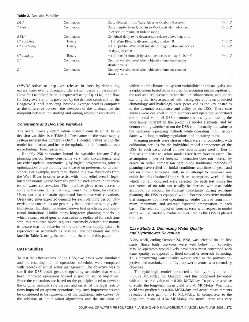
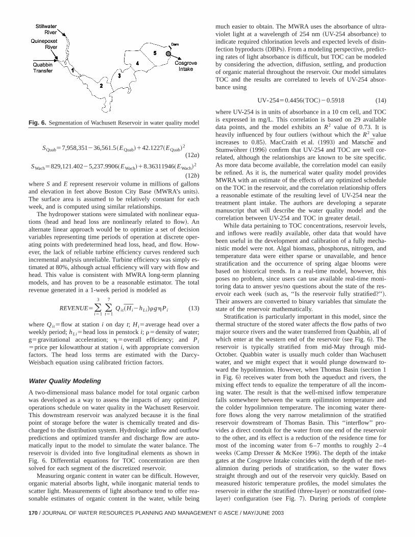
Table 2. Decision Variables

DIVi Continuous Daily diversion from Ware River to Quabbin Reservoir i 51–7TRANi Continuous Daily transfer from Quabbin to Wachusett via hydroplant

in excess of minimum turbine ratingi 51–7

REL1 Continuous Combined daily extra downstream release above req. min.CheckDiv i Binary 51 if Ware River is diverted on dayi, else50 i 51–7CheckTrani Binary 51 if Quabbin-Wachusett transfer through hydroplant occurs

on dayi, else50i 51–7

CheckBypi Binary 51 if transfer through bypass pipe occurs on dayi, else50 i 51–7Z1 Continuous Dummy variable used when objective function contains

absolute valueZ2 Continuous Dummy variable used when objective function contains

absolute value

gre

th

th.

8

a

ayntomo-r-

dnt

icr

nt

b

teretusl-

ca

f

ofder-tedesseandheyto

r-

theofeilyofdyngheleeleni-cheled

st,hg.b-ary

fy

ttntsey

~MWRA strives to keep extra releases in check by distributinexcess water evenly throughout the system, based on basin a!.Flow for Oakdale Station is expressed using Eq.~11a!, and flowfor Cosgrove Station is governed by the demand constraint forCosgrove Tunnel~servicing Boston!. Average head is computedas the difference between the elevation of the turbines andmidpoint between the starting and ending reservoir elevations

Constraints and Decision Variables

The overall weekly optimization problem consists of 36 to 3decision variables~see Table 2!. The nature of the water supplysystem necessitates numerousON/OFF control values within themodel formulation, and hence the optimization is formulated asmixed-integer linear program.

Roughly 250 constraints bound the variables for any 7-dplanning period. Some constraints vary with circumstance, aare either updated automatically by logical programming prioroptimization, or are input by users based on preference or circustance. For example, users may choose to allow diversions frthe Ware River in order to assist with flood relief even if legislated constraints would normally prohibit such action in the inteest of water conservation. The interface gives users accesssome of the constraints that may, from time to time, be relaxeUsers can also constrain upper and lower reservoir elevatioUsers also enter expected demand for each planning period. Oerwise, the constraints are generally fixed, and represent physlimitations, legislated mandates, known best practices, and opetional limitations. Unlike many long-term planning models, inwhich a small set of general constraints is replicated for each timstep, this real-time model requires extremely detailed constraito ensure that the behavior of the entire water supply systemreproduced as accurately as possible. The constraints are talated in Table 3, using the notation at the end of this paper.

Case Studies

To test the effectiveness of the DSS, two cases were simulaand the resulting optimal operations schedules were compawith records of actual water management. The objective wassee if the DSS could generate operating schedules that wohave improved operations toward a specific set of objectiveSince the constraints are based on the principles used to devethe original monthly rule curves, and on all of the legal restrictions imposed on system operations, any such improvementsbe considered to berefinementsof the traditional rule curves~bythe addition of optimization algorithms and the inclusion o


a

e

e

d

-m

to.s.h-ala-

esisu-

dd

old.op

n

within-month climate and system variabilities in the analysis!, nota replacement based on new rules. Overcoming misperceptionsthe tool as a replacement rather than an enhancement, and unstanding the risks associated with basing operations on predicclimatology and hydrology, were perceived as the key obstaclto the eventual acceptance and utility of the DSS. These castudies were designed to help planners and operators understthe potential value of DSS recommendations by addressing tuncertainty inherent in the predictive model elements, and bdemonstrating whether or not the DSS could actually add valuethe traditional operating methods while operating in full accodance with long-standing regulations and operating rules.

Planning periods were chosen which were not coincident wicalibration periods for the individual model components of thDSS. In each case, actual climate records were used in lieuforecasts in order to isolate model error from forecast error. Thassumption of perfect forecast information does not necessarcreate an unfair comparison here, since traditional methodsplanning have relied on initial conditions and time of year, annot on climate forecasts. Still, in an attempt to minimize anunfair benefits obtained from such an assumption, weeks duriwhich no rain occurred were selected for each test, since toccurrence of no rain can usually be forecast with reasonabaccuracy. To account for forecast uncertainty during real-timplanning, the DSS is equipped with a forecast sensitivity moduthat compares optimized operating schedules derived from mimum, maximum, and average expected precipitation in eabasin. The relative impact of forecast error with respect to moderrors will be carefully evaluated over time as the DSS is phasinto use.

Case Study 1: Optimizing Water Qualityand Hydropower Revenues

A dry week, ending October 24, 1998, was selected for the firstudy. Since both reservoirs were well below full capacityMWRA operators would likely have been most concerned witwater quality, as opposed to flood control or reservoir balancinThus maximizing water quality was selected as the primary ojective, and maximization of hydropower revenues as a secondobjective.

The hydrologic models predicted a net hydrologic loss o20.072 MCM/day for Quabbin, and this compared favorablwith a measured value of20.064 MCM/day. To provide a senseof scale, the long-term mean yield is 0.78 MCM/day. Wachuseyield was predicted as 0.064 MCM/day, and actual measuremerevealed a true gain of 0.10 MCM/day. In comparison to thlong-term mean of 0.54 MCM/day, the model error was ver


0

e

by

er

Table 3. Model Constraints

Type Constraint Notes

Capacity Sk.Sk-min

Hydraulic Qix9 ,Qx-max

Flooding FSk2Sk-max

7 G1RDS2k1RELk1<FCk

Term in brackets represents daily spill

Water quality CheckTrani 1CheckBypi5@1,—# Force transfer from 5/1 to 10/30

CheckTrani 1CheckBypi5@1,—# Force transfer if water in Quabbin Aqueduct is stagnant for 3days

Legislated DIVi 5@0,—# Diversions are not allowed from 6/15 to 10/14

DIVi<QWare20.32MCM/day Can only divert Ware flow in excess of 85 mgd~minimuminstream flow!

[email protected],0.17,0.27#8 MCM/day Minimum release to Swift River is governed by predicted flow inConnecticut River

Operational DIVi 5@0,—# Cannot divert Ware River if Quabbin is aboveNORM

REL15@0,—# Can only release extra water if both res. aboveNORM

DIVi , TRANi , REL1, Z1, Z2>0 Continuous decision variables cannot be negative

Binary CheckDivi , CheckTrani , CheckByp5@0,1# Definition of binary decision variables

CheckDivi 1CheckTrani1CheckByp<1 Quabbin Aqueduct can only be used for one purpose at a tim

DIVi 2CheckDivi>20.999 If DIVi50, this forcesCheckDiv i50

1000* CheckDivi2DIV>0 If DIVi.0, this forcesCheckDiv i51

TRANi2CheckTrani>20.999 If TRANi50, this forcesCheckTrani50

1000* CheckTrani2TRANi>0 If TRANi.0, this forcesCheckTrani51

Hydrology Qi5Qi8 Hydrology constrained by model predictionsEk5Ek8

SPk5SPk8 @see Eqs.~2!–~7!#

Demand Ry5Ry

Water balanceSkt5Skt211(

i(j,x

Inflowj,x2(i(x,y

Outflowx,y

Reference Eqs.~9!–~10b!

Hydropower Pz5Qz9(Hz2hz2)rg Reference Eq.~7!

Unusual operations CheckBypi5@0,—# Can force any transfers through the hydrostation at Oakdaledisallowing bypass flow

DIVi5@MIN(MAX constraints* ),—# Can force Ware diversions if necessary to reduce Ware Rivflooding*Not all max constraints apply, as this option overridesminimum instream flow and Quabbin volume constraints

DIVi5@MIN(MAX constraints),—# If Ware River diversions are allowable, divert the maximumallowable amount

Absolute values SWach2Target2Z11Z250 DefinesZ1 andZ2 when optimizing Wachusett volume towarda target

@(SQuab2SNORM-Q)/SNORM-Q#2@(SWach2SNORM-W)/SNORM-W#2Z11Z250

DefinesZ1 andZ2 when balancing reservoirs

daeee

nns

d-

ues

to

e

small. These yield prediction errors are orders of magnitusmaller than typical operational flows, and were thereforesumed to have very little influence on the results. The modpredicted the correct hydrologic regime for the Connecticut Rivand hence minimum downstream releases from Quabbin waccurately constrained.

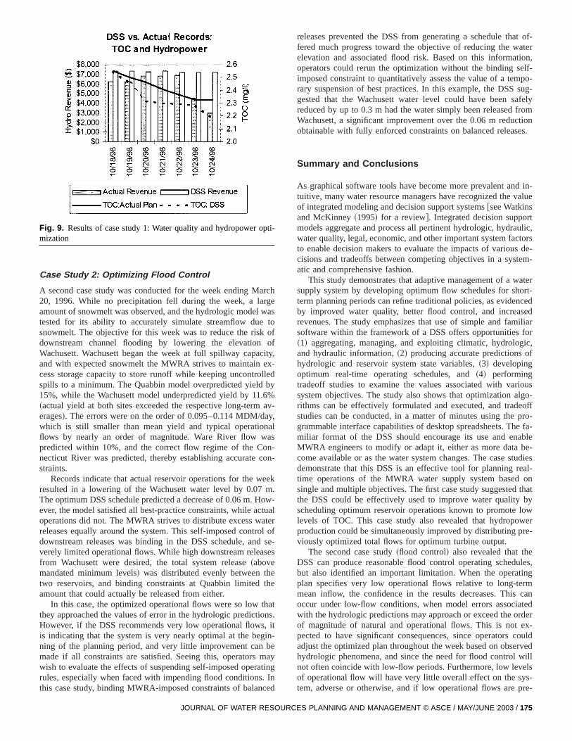
Fig. 9 illustrates the effectiveness of the DSS in optimiziboth objectives with hierarchical prioritization. Actual operatioreduced TOC concentration in the receiving basin of Wachu


es-lsr,re

gsett

by roughly 8%, while optimized operations could have reduceTOC concentration by 14%. At the same time, by optimally distributing the total transfers~optimized for water quality! over 7days, the DSS schedule increased simulated hydropower revenby roughly 20%, or $10,000 for the week~actual revenues werecorrected based on the assumed efficiency of 80% in ordercompare identical systems!. Hydropower could have been in-creased further, but the optimized flows for water quality werbinding constraints in this secondary optimization.


of-tern,

lf-po-ug-felyomons.

in-lue

lic,rs

ti-
Fig. 9. Results of case study 1: Water quality and hydropower opmization
arcgewatooof

cityex-lleby

.6%a

ay,nalas

on-con

eemowtu

ateol od sses

ethe

thaons, itinbematin

. Inced

de-m-

terrt-edd

iliarr

c,

uso-

offro-fa-

blee-diesl-n

hatywer

e-

les,g

caneder

x-uld

vedills-e-


h

s

f

,

d

v-

-

k.

-alrfe-

t.

-

yg

releases prevented the DSS from generating a schedule thatfered much progress toward the objective of reducing the waelevation and associated flood risk. Based on this informatiooperators could rerun the optimization without the binding seimposed constraint to quantitatively assess the value of a temrary suspension of best practices. In this example, the DSS sgested that the Wachusett water level could have been sareduced by up to 0.3 m had the water simply been released frWachusett, a significant improvement over the 0.06 m reductiobtainable with fully enforced constraints on balanced release

Summary and Conclusions

As graphical software tools have become more prevalent andtuitive, many water resource managers have recognized the vaof integrated modeling and decision support systems@see Watkinsand McKinney~1995! for a review#. Integrated decision supportmodels aggregate and process all pertinent hydrologic, hydrauwater quality, legal, economic, and other important system factoto enable decision makers to evaluate the impacts of variouscisions and tradeoffs between competing objectives in a systeatic and comprehensive fashion.

This study demonstrates that adaptive management of a wasupply system by developing optimum flow schedules for shoterm planning periods can refine traditional policies, as evidencby improved water quality, better flood control, and increaserevenues. The study emphasizes that use of simple and famsoftware within the framework of a DSS offers opportunities fo~1! aggregating, managing, and exploiting climatic, hydrologiand hydraulic information,~2! producing accurate predictions ofhydrologic and reservoir system state variables,~3! developingoptimum real-time operating schedules, and~4! performingtradeoff studies to examine the values associated with variosystem objectives. The study also shows that optimization algrithms can be effectively formulated and executed, and tradestudies can be conducted, in a matter of minutes using the pgrammable interface capabilities of desktop spreadsheets. Themiliar format of the DSS should encourage its use and enaMWRA engineers to modify or adapt it, either as more data bcome available or as the water system changes. The case studemonstrate that this DSS is an effective tool for planning reatime operations of the MWRA water supply system based osingle and multiple objectives. The first case study suggested tthe DSS could be effectively used to improve water quality bscheduling optimum reservoir operations known to promote lolevels of TOC. This case study also revealed that hydropowproduction could be simultaneously improved by distributing prviously optimized total flows for optimum turbine output.

The second case study~flood control! also revealed that theDSS can produce reasonable flood control operating schedubut also identified an important limitation. When the operatinplan specifies very low operational flows relative to long-termmean inflow, the confidence in the results decreases. Thisoccur under low-flow conditions, when model errors associatwith the hydrologic predictions may approach or exceed the ordof magnitude of natural and operational flows. This is not epected to have significant consequences, since operators coadjust the optimized plan throughout the week based on obserhydrologic phenomena, and since the need for flood control wnot often coincide with low-flow periods. Furthermore, low levelof operational flow will have very little overall effect on the system, adverse or otherwise, and if low operational flows are pr

Case Study 2: Optimizing Flood Control

A second case study was conducted for the week ending M20, 1996. While no precipitation fell during the week, a laramount of snowmelt was observed, and the hydrologic modeltested for its ability to accurately simulate streamflow duesnowmelt. The objective for this week was to reduce the riskdownstream channel flooding by lowering the elevationWachusett. Wachusett began the week at full spillway capaand with expected snowmelt the MWRA strives to maintaincess storage capacity to store runoff while keeping uncontrospills to a minimum. The Quabbin model overpredicted yield15%, while the Wachusett model underpredicted yield by 11~actual yield at both sites exceeded the respective long-termerages!. The errors were on the order of 0.095–0.114 MDM/dwhich is still smaller than mean yield and typical operatioflows by nearly an order of magnitude. Ware River flow wpredicted within 10%, and the correct flow regime of the Cnecticut River was predicted, thereby establishing accuratestraints.

Records indicate that actual reservoir operations for the wresulted in a lowering of the Wachusett water level by 0.07The optimum DSS schedule predicted a decrease of 0.06 m. Hever, the model satisfied all best-practice constraints, while acoperations did not. The MWRA strives to distribute excess wreleases equally around the system. This self-imposed contrdownstream releases was binding in the DSS schedule, anverely limited operational flows. While high downstream releafrom Wachusett were desired, the total system release~abovemandated minimum levels! was distributed evenly between thtwo reservoirs, and binding constraints at Quabbin limitedamount that could actually be released from either.

In this case, the optimized operational flows were so lowthey approached the values of error in the hydrologic predictiHowever, if the DSS recommends very low operational flowsis indicating that the system is very nearly optimal at the begning of the planning period, and very little improvement canmade if all constraints are satisfied. Seeing this, operatorswish to evaluate the effects of suspending self-imposed operarules, especially when faced with impending flood conditionsthis case study, binding MWRA-imposed constraints of balan


t th

ultsot toea-

nceea-g,

f thehichtestctiveded

plantheccuplan

eduThe

usendaedlti-thethe

oodsup

t-

dadcon

ac-e o

li-npu

liabs a

n-hapto

ortes-andandtfulual-

i-

s-od-

f

-s in

east

ip, H.on

. E.hy-for-

rt

scribed, the system can be considered to be nearly optimal astart of the period.

Still, a DSS solves only part of the decision problem. Resfrom a DSS are intended to guide and support decisions, nmake them, and in such a role, the true utility of a DSS is msured in part by the comfort level of those who use it. Oaccepted by the users, its reliability can then only be fully msured with actual use over time. At the time of this writinMWRA personnel have been testing the predictive strength ohydrologic model elements against very recent records, wwere unavailable during the development of the tool. Thesehave been designed to build confidence in the model’s prediaccuracy, so that its ultimate output, in the form of recommenoperating schedules, can be considered to be reliable.

The DSS has been used occasionally to support generalning decisions, but its full implementation is not planned untilhydrologic models have demonstrated enough predictive aracy, based on recent records, to satisfy both operators andners. Recent world events, unfortunately, set the testing schback, as the MWRA refocused its attention on security issues.current plan is to complete the hydrologic verification, thenthe model in a hypothetical mode by comparing its recommetions against actual operations~additional case studies, conductin real time! for a period of several weeks or months, and umately to make the tool available to those who will makedaily and weekly operational decisions. We believe thatMWRA’s approach to the implementation of the model is a gexample for others considering the development of decisionport tools.1. The MWRA will build confidence in the model by conduc

ing additional verification tests on key model elements;2. The MWRA will compare results from the fully integrate

model against traditional operations as decisions are mand results measured, further evaluating accuracy andsistency;

3. Any required refinements or recalibration can be easilycomplished by MWRA engineers and planners becausthe familiarity of the software;

4. The MWRA is identifying reliable sources of real-time cmate data and forecasts so that weekly collection and iof data can become nearly automatic;

5. Once the model has demonstrated its robustness and reity, it will become available to planners and operators atool for refining traditional rule-curve decisions. It is itended for guidance only, and not as a mandate. Permore clearly, it is intended by the authors and by MWRAsupplement operator judgment, not to replace it.

Acknowledgments

The writers wish to thank the following people from MWRA ftheir advice and technical support of this work: Steven EsSmargiassi, Daniel Nvule, Marcis Kempe, Windsor Sung,Guy Foss. We also thank Charles Howard for his inspiration,two anonymous reviewers for their perceptive and thoughcomments, the inclusion of which helped improve both the qity and focus of this work.

Constraint Notation

Indicesi 5 daily index (i 51 – 7);


e

s

-

--

le

-

-

e-

f

t

il-

s

j 5 basin index~Quabbin, Wachusett, Ware, Connecti-cut!;

k 5 reservoir index~Quabbin, Wachusett!;t 5 weekly index;x 5 operational flow index~transfers, diversions, extra

releases!;y 5 demand index~Cosgrove Aqueduct, Wachusett

Aqueduct, Chicopee Valley Aqueduct, etc.!; andz 5 hydropower station index.

AbbreviationsDS 5 downstream;

E 5 daily surface evaporation;FC 5 flood capacity;

H 5 head;h2 5 head loss;

NORM5 normal volume;P 5 power;Q 5 natural streamflow~daily!;

Q9 5 operational flow~daily!;R 5 daily release;S 5 final storage; and

SP 5 daily seepage.

Other@a,b# 5 different values apply at different times or are cond

tional on logical comparisons;ValueI 5 user input;

— 5 no constraint; and8 5 model prediction.

References

Alley, W. M. ~1984!. ‘‘On the treatment of evapotranspiration, soil moiture accounting, and aquifer recharge in monthly water balance mels.’’ Water Resour. Res.,20~8!, 1137–1149.

Beven, K. ~1989!. ‘‘Changing ideas in hydrology—The case ophysically-based models.’’J. Hydrol.,105, 159.

Camp Dresser & McKee, Inc.~1996!. ‘‘Wachusett Reservoir water treatment plan EIR/conceptual design: Understanding algal dynamicWachusett Reservoir to manage taste and odor.’’Rep. Prepared forMassachusetts Water Resources Authority, Boston.

Cohon, J. L., and Marks, D. H.~1975!. ‘‘A review and evaluation ofmultiobjective programming techniques.’’Water Resour. Res.,11~2!,208–220.

Fennessey, N. M., and Vogel, R. M.~1996!. ‘‘Regional models of poten-tial evaporation and reference evapotranspiration for the northUSA.’’ J. Hydrol.,184, 337–354.

Fernandez, W., Vogel, R. M., and Sankarasubramanian, A.~2000!. ‘‘Re-gional calibration of a watershed model.’’Hydrol. Sci. J.,45~5!, 689–707.

Hargreaves, G. H., and Samani, Z. A.~1982!. ‘‘Estimating potentialevapotranspiration.’’J. Irrig. Drain Eng., 108~3!, 225–230.

Hooper, R. P., Stone, A., Christophersen, N., de Grosbois, E., and SeM. ~1988!. ‘‘Assessing the Birkenes model of stream acidificatiusing a multisignal calibration methodology.’’Water Resour. Res.,24,1308–1316.

Hornberger, G. M., Beven, K. J., Cosby, B. J., and Sappington, D~1985!. ‘‘Shenandoa watershed study: Calibration of a topograpbased, variable contributing area hydrological model to a smallested catchment.’’Water Resour. Res.,21, 1841–1859.

Jakeman, A. J., and Hornberger, G. M.~1993!. ‘‘How much complexity iswarranted in a rainfall-runoff model.’’Water Resour. Res.,29~8!,2637–2649.

Loucks, D. P.~1995!. ‘‘Developing and implementing decision supposystems: A critique and a challenge.’’Water Resour. Bull.,31~4!, 571–582.


J.e-

l,

,

s-l,

m,

t-ufts

MacCraith, B., Grattan, K. T. V., Connolly, D., Briggs, R., Boyle, W.O., and Avis, M. ~1993!. ‘‘Cross comparison of techniques for thmonitoring of total organic carbon~TOC! in water sources and supplies.’’ Water Sci. Technol.,28~11-12!, 457–463.

Matsche, N., and Stumwo¨hrer, K. ~1996!. ‘‘UV absorption as controparameter for biological treatment plants.’’Water Sci. Technol.33~12!, 211–218.

Revelle, C. S., Whitlatch, E. E., and Wright, J. R.~1997!. Civil andenvironmental systems engineering, Prentice-Hall, Englewood CliffsN.J., Chap. 10.

Shuttleworth, W. J., and Maidment, D. R., eds.~1993!. ‘‘Chapter 4:Evaporation.’’ Handbook of hydrology, McGraw-Hill, New York,4.18, 4.31.


Thomas, H. A.~1981!. ‘‘Improved methods for national water assesment.’’ Rep., Contract WR 15249270, U.S. Water Resources CounciWashington, D.C.

Vanderwiele, G. L., Xu, C.-Y., and Yang, J.-C.~1992!. ‘‘Methodology andcomparative study of monthly water balance models in BelgiuChina and Burma.’’J. Hydrol.,134, 315–347.

Vogel, R. M., and Hellstrom, D. I.~1988!. ‘‘Long range surface watersupply planning.’’Civ. Eng. Pract., BSCES,3~1!, 7–26.

Watkins, D. W., Jr., and McKinney, D. C.~1995!. ‘‘Recent developmentsassociated with decision support systems in water resources.’’Rev.Geophys.,33, supplement, 941–948.

Westphal, K. S.~2001!. ‘‘A real-time decision support model for operaing the eastern Massachusetts water supply system.’’ MS thesis, TUniv., Medford, Mass.


Decision Support System for Adaptive Water Supply...

Documents

Transcript of Decision Support System for Adaptive Water Supply...