DECISION MODELING WITH DECISION MODELING WITH MICROSOFT EXCELMICROSOFT EXCEL

Copyright 2001Prentice Hall

DECISIONDECISION

Chapter 8Chapter 8

ANALYSISANALYSISPart 1Part 1

DECISION ANALYSISDECISION ANALYSISIntroductionIntroductionDecision analysis provides a framework for analyzing a wide variety of management models. The framework establishes

1. A system of classifying decision models based on the amount of information about the model that is available 2. A decision criterion (a measure of the

“goodness” of fit). Decision analysis treats decisions against nature (outcomes over which you have no control) and the returns accrue only to the decision maker.

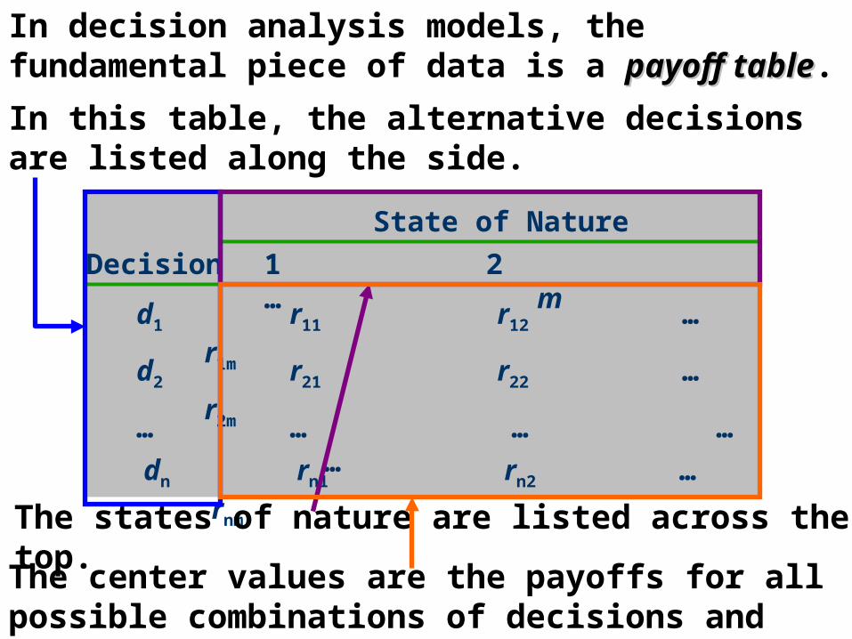
In decision analysis models, the fundamental piece of data is a payoff tablepayoff table.

State of Nature

1 2 … m

Decision

d1 r11 r12 … r1m

d2 r21 r22 … r2m

dn rn1 rn2 … rnm

… … … … …

In this table, the alternative decisions are listed along the side.

The states of nature are listed across the top.The center values are the payoffs for all possible combinations of decisions and states of nature.

The decision process is as follows:

1. Select one of the alternative decisions (di). 2. After your decision is made, a state of nature occurs that is beyond your control. 3. The associated return can then be determined from the payoff table (rij).

The decision that we select depends on our belief concerning what nature will do (i.e., which state of nature will occur).

To help us make the decision, several assumptions about nature’s behavior will be made. Each assumption leads to a different criterioncriterion for selecting the “best” decision.

DECISION ANALYSISDECISION ANALYSISThree Classes of Decision ModelsThree Classes of Decision ModelsThe three classes are

Decisions Under Risk

Decisions Under Uncertainty

Decisions Under Certainty

DECISIONS UNDER CERTAINTYDECISIONS UNDER CERTAINTY

A decision under certaintydecision under certainty is one in which you know (with certainty) which state of nature will occur.

For example, in the morning you are deciding whether to take your umbrella to work and you know for sure that it will be raining when you leave work in the afternoon.The payoff table for this model is:

RainTake Umbrella 0Do Not -7.00

It costs $7.00 to have your suit cleaned if you get caught in the rain.

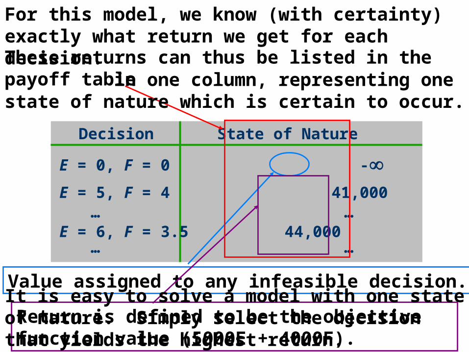
All LP, ILP and NLP models as well as other deterministic models such as the EOQ model can be thought of as decisions against nature in which there is only one state of nature.For example, consider the following LP model: Max 5000E + 4000F

s.t. 10E + 15F < 150

20E + 10F < 160

30E + 10F > 135

E – 3F < 0

E + F > 5

E, F > 5

State of NatureDecision

E = 0, F = 0 -E = 5, F = 4 41,000

E = 6, F = 3.5 44,000… …

… …

Value assigned to any infeasible decision.

Return is defined to be the objective function value (5000E + 4000F).

For this model, we know (with certainty) exactly what return we get for each decision.These returns can thus be listed in the payoff table in one column, representing one state of nature which is certain to occur.

It is easy to solve a model with one state of nature. Simply select the decision that yields the highest return.

DECISIONS UNDER RISKDECISIONS UNDER RISK

In most models, there is a lack of certainty about future events. In quantitative modeling, the lack of certainty can be dealt with in various ways. Definition of Risk: Definition of Risk: RiskRisk refers to a class of decision models for which there is more than one state of nature.

In addition, we assume that there is a probability estimate for the occurrence of each of the various states of nature.

The probability of state of nature j occurring is generally estimated using historical frequencies. Otherwise, subjective estimates are made.

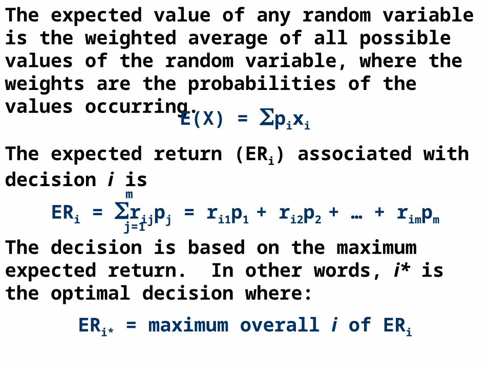
The expected value of any random variable is the weighted average of all possible values of the random variable, where the weights are the probabilities of the values occurring.

The expected return (ERi) associated with decision i is

E(X) = pixi

The decision is based on the maximum expected return. In other words, i* is the optimal decision where:

ERi* = maximum overall i of ERi

ERi = rijpj = ri1p1 + ri2p2 + … + rimpmj=1

m

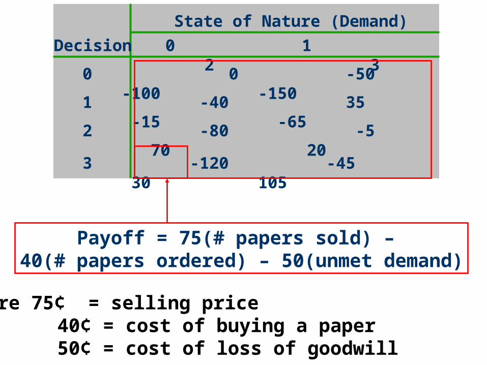
The Newsvendor Model: The Newsvendor Model: A newsvendor can buy the Wall Street Journal newspapers for 40 cents each and sell them for 75 cents.

However, he must buy the papers before he knows how many he can actually sell. If he buys more papers than he can sell, he disposes of the excess at no additional cost. If he does not buy enough papers, he loses potential sales now and possibly in the future.Suppose that the loss of future sales is captured by a loss of goodwill cost of 50 cents per unsatisfied customer.

The demand distribution is as follows:

P0 = Prob{demand = 0} = 0.1

P1 = Prob{demand = 1} = 0.3

P2 = Prob{demand = 2} = 0.4

P3 = Prob{demand = 3} = 0.2

Each of these four values represent the states of nature. The number of papers ordered is the decision. The returns or payoffs are as follows:

State of Nature (Demand)

0 1 2 3

Decision

0 0 -50 -100 -1501 -40 35 -15 -652 -80 -5 70 203 -120 -45 30 105

Payoff = 75(# papers sold) – 40(# papers ordered) – 50(unmet demand)

Where 75¢ = selling price 40¢ = cost of buying a paper 50¢ = cost of loss of goodwill

Now, the ER is calculated for each decision i :

State of Nature (Demand)

0 1 2 3

Decision

0 0 -50 -100 -150 -85 1 -40 35 -15 -65 -12.52 -80 -5 70 20 22.53 -120 -45 30 105 7.5

ER

Prob. 0.1 0.3 0.4 0.2

ER1 = -40(0.1) + 35(0.3) – 15(0.4) – 65(0.2) = -12.5

ER2 = -80(0.1) – 5(0.3) + 70(0.4) + 20(0.2) = 22.5

ER3 = -120(0.1) – 45(0.3) + 30(0.4) – 105(0.2) = 7.5

ER0 = 0(0.1) – 50(0.3) – 100(0.4) – 150(0.2) = -85

Of these four ER’s, choose the maximum,and order 2 papers

Another way to compare the decisions is to look at a graph of their risk profiles:

The risk profilerisk profile shows all the possible outcomes with their associated probabilities for a given decision and graphically aids in decision making.

The Cost of Lost Goodwill: The Cost of Lost Goodwill: A Spreadsheet Sensitivity Analysis A Spreadsheet Sensitivity Analysis This decision is based on the cost of lost goodwill, whose value is much less certain than selling price and purchase cost.

Now, perform a sensitivity analysis to determine what would happen to the optimal decision if the cost of lost goodwill were different.An Excel spreadsheet is highly suitable to calculate the payoff matrix and expected returns.

Here is the spreadsheet model for the decision table:

=$B$1*MIN($A7,B$6)-$B$2*$A7- $B$3*MAX(B$6-$A7,0)

=SUMPRODUCT(B7:E7,$B$12:$E$12)

Using the Data Table command, a table of expected returns can easily be generated for a range of Goodwill Costs.

After copying the entire

“Base Case” into a new

worksheet, enter 0 in cell

A16, then click on Edit – Fill –

Series – Series in Columns with a step value of

5.

=F7=F8=F9=F10

Click on Data – Table and enter $B$3 as the column input cell.

Now, graph the result of the Data Table to help sort out all the numbers.

Highlight the range of data (A16:E46) and click on the Chart Wizard icon. In the resulting dialog, choose the Line graph and click Next. In the next dialog, click on the Series tab and indicate that the Category (X) axis labels are found in A16:A46.

Click Next and enter titles or labels for the graph.Click Finish when done to display the graph.

Here is the resulting graph.

-300

-250

-200

-150

-100

-50

0

50

0 10 20 30 40 50 60 70 80 90 100

110

120

130

140

150

Goodwill Cost (cents)

Exp

ect

ed

Re

turn

(ce

nts

)

Order 0

Order 1

Order 2

Order 3

For a Goodwill Cost less than 125 cents, the optimal decision is to order 2 papers.For a Goodwill Cost of 125 cents, alternative optima exists: order 2 or 3 papers.

DECISIONS UNDER UNCERTAINTYDECISIONS UNDER UNCERTAINTY

In decisions under uncertaintydecisions under uncertainty, there is more than one possible state of nature. However, now the decision maker is unwilling or unable to specify the probabilities that the various states of nature will occur. In this case, there are several approaches.Laplace Criterion: Laplace Criterion: The Laplace criterion approach interprets the condition of “uncertainty” as equivalent to assuming that all states of nature are equally likely to all states of nature are equally likely to occuroccur. For example, in the newsvendor model, assuming all states are equally likely means that since there are four states, each state occurs with probability 0.25.

Using the Laplace (equally likely) criterion, here are the resulting returns:

Each state of nature has equal probability of occurring =

0.25

Choosethe max.return

Then, the decision that yields the maxmaximum value of the minminimum returns (maximin) is selected.

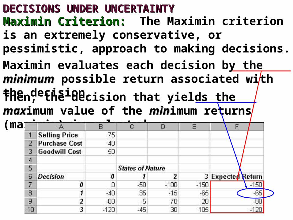
DECISIONS UNDER UNCERTAINTYDECISIONS UNDER UNCERTAINTYMaximin Criterion: Maximin Criterion: The Maximin criterion is an extremely conservative, or pessimistic, approach to making decisions.

Maximin evaluates each decision by the minimumminimum possible return associated with the decision.

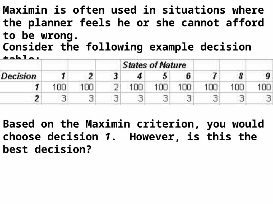
Maximin is often used in situations where the planner feels he or she cannot afford to be wrong.Consider the following example decision table:

Based on the Maximin criterion, you would choose decision 1. However, is this the best decision?

The decision that yields the maxmaximum of these maxmaximum returns (maximax) is then selected.

This method evaluates each decision by the maximummaximum possible return associated with that decision.

DECISIONS UNDER UNCERTAINTYDECISIONS UNDER UNCERTAINTYMaximax Criterion: Maximax Criterion: The Maximax criterion is an optimistic decision making criterion.

Consider the following example decision table:

Based on the Maximax criterion, you would choose decision 2. However, is this the best decision?

DECISIONS UNDER UNCERTAINTYDECISIONS UNDER UNCERTAINTYRegret and Minimax Regret: Regret and Minimax Regret: Regret measures the desirability of an outcome. The decision is made on the least regret for making that choice.So far, all the decision criteria have been used on a payoff table of dollar returns as measured by net cash flows.

The following table shows the regret for each combination of decision and state of nature.

The calculated regret indicates how much better we can do as far as making a choice. “Regret” is synonymous with the “opportunity cost” of not making the best decision for a given state of nature.

State of Nature

0 1 2 3

Decision

0

1

2

3

0 - = 0

0 – ( ) = 40

0 – ( ) = 80

0 – ( ) = 120

To build the Regret table, first choose the maximum value in columncolumn 1:

0

-40

-80

-120

Now, subtract every value in that column from this value:The resulting values are the regrets for the associated decision and state of nature.

Repeat these steps for the remaining columns.

85

0

40

80

170

85

0

40

255

170

85

0

State of Nature (Demand)

0 1 2 3

Decision

0 0 85 170 255 1 40 0 85 1702 80 40 0 853 120 80 40 0

Max. Regret

Once the Regret table is built, choose the maximum value in each row:

255

170

85

120

Then, of these maximum values, choose the smallest [i.e., the decision that minminimizes the maxmaximum regret (minimax criterion)].

DECISIONS UNDER UNCERTAINTYDECISIONS UNDER UNCERTAINTYSo, using the 3 criteria under uncertainty, we made the following decisions regarding the newsvendor data:

CriteriaCriteria Decision Decision

Maximin Cash Flow Order 1 paper

Note that when making decisions without probabilities, the three criteria listed above can result in different “optimal” solutions.

Maximax Cash Flow Order 3 papers

Minimax Regret Order 2 papers

DECISION ANALYSISDECISION ANALYSISThe Expected Value of Perfect The Expected Value of Perfect Information: Newsvendor Model Information: Newsvendor Model Under RiskUnder RiskLet’s return to the newsvendor model under risk (with the known probability distribution on demand) in order to introduce the concept of the expected value of perfect information.The newsvendor, without knowing the actualactual demand, orders the newspapers based on the distribution of demand. At the end of the day, the demand is revealed to the newsvendor and an actualactual return can be determined by his order-size decision and the demand.

What if, the newsvendor can purchase “perfect information” on the demand for his newspapers which would enable him to make better decisions?

The question that we need to answer is: What is the largest fee the newsvendor should be willing to pay for this perfect information? This fee is called the expected value of expected value of perfect information perfect information (EVPI):

EVPI = (expected return with new deal) – (expected return with current sequence of

events)The EVPI gives an upper bound on the amount that you should be willing to pay for the “perfect information.”

To calculate the expected return with the new deal, choose the maximum value for each outcome (column) and multiply it by its respective probability. Then, add the resulting products.

With perfect information, the newsvendor will always order the number of papers that will give him the maximum return for the state of nature that will occur.

However, the payment for this information must be made before the newsvendor learns what the demand will be.

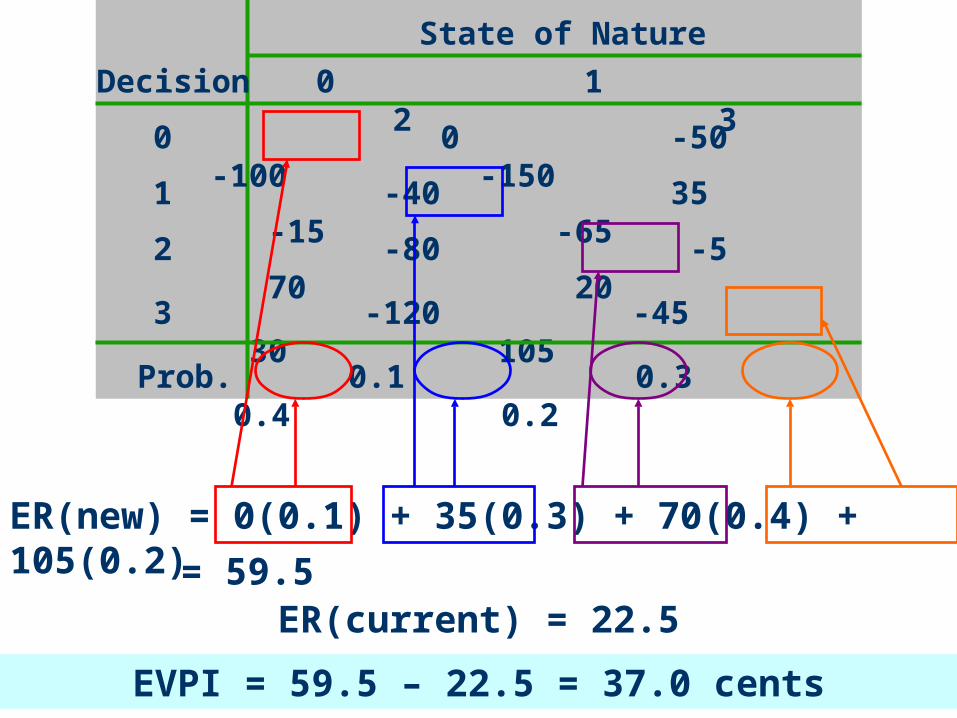
ER(new) = 0(0.1) + 35(0.3) + 70(0.4) + 105(0.2)

State of Nature

0 1 2 3

Decision

0 0 -50 -100 -1501 -40 35 -15 -652 -80 -5 70 203 -120 -45 30 105

Prob. 0.1 0.3 0.4 0.2

= 59.5ER(current) = 22.5

EVPI = 59.5 – 22.5 = 37.0 cents

DECISION ANALYSISDECISION ANALYSISUtilities and Decisions under RiskUtilities and Decisions under RiskUtilityUtility is an alternative way of measuring the attractiveness of the result of a decision. It is an alternative way of finding the values to fill in a payoff table.

Previously, we used net dollar return (net cash flow) and regret as two measures of the “goodness” of a particular combination of a decision and state of nature.

Utility suggests another type of measure.

Consider the following game in which an urn contains 99 white balls and 1 black ball. A single ball is drawn from the urn. Each ball is equally likely to be drawn.

THE RATIONALE FOR UTILITYTHE RATIONALE FOR UTILITY

If a white ball is drawn, you must pay $10,000. If the black ball is drawn, you receive $1,000,000. You must decide whether to play.

PlayDo Not Play

DECISIONSTATE OF NATURE

White Ball Black Ball

-10,000 1,000,000 0 0

The payoff table is:

The probability of a white and a black ball are 0.99 and 0.01, respectively. The expected returns are:ER(play) = -10,000(0.99) + 1,000,000(0.01) = -9900 + 10,000 = 100

ER(do not play) = 0(0.99) + 0(0.01) = 0

Since ER(play) > ER(do not play), you should play if the criterion of maximizing the expected net cash flow is applied.

So, will you play this game?

This simple example shows that you need to take care in selecting an appropriate criterion.

Most people are risk-averserisk-averse, which means they would feel that the loss of a certain amount of money would be more painful than the gain of the same amount of money. Utility function Utility function in decision analysis measures the “attractiveness” of money. UtilityUtility can be thought of as a measure of “satisfaction.” Two characteristics are:

1. It is nondecreasing, since more money is always at least as attractive as less money.2. It is concave (the marginal utility of money is nonincreasing).

To illustrate, first suppose you have $100 and someone gives you an additional $100. Note that your utility increases by

U(200) – U(100) = 0.680 – 0.524 = 0.156

Now suppose you start with $400 and someone gives you an additional $100. Now your utility increases by

U(500) – U(400) = 0.910 – 0.850 = 0.060

This illustrates that an additional $100 is less attractive if you have $400 on hand than it is if you start with $100.

The gain of a specified number of dollars increases utility less than the loss of the same number of dollars decreases utility.

Utility

1.00.9100.8500.775

0.680

0.524

100 200 300 400 500 600 Dollars

Typical risk-averse utility function:

Go from $400 to $500 results

in

A gain in

utility of

0.06

Go from $400 to $300 results

in

A loss in

utility of

0.075

Utility

1.0

0.590

0.260

0.075

100 200 300 400 Dollars

Risk-seeking (convex) function:

A gain of a specified amount of dollars increases the utility more than a loss of the same amount of dollars decreases the utility.

Go from $200 to $300 results

in

A gain in

utility of

0.330

Go from $200 to $100 results

in

A loss in

utility of

0.185

Utility

1.0 0.90

0.60

0.30 100 200 300 400 Dollars

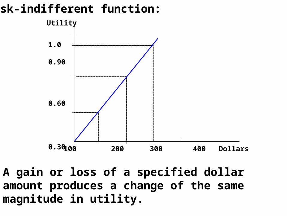
Risk-indifferent function:

A gain or loss of a specified dollar amount produces a change of the same magnitude in utility.

To begin, arbitrarily select the endpoints of the utility function.

CREATING AND USING A UTILITY FUNCTIONCREATING AND USING A UTILITY FUNCTION

For convenience, set the utility of the smallest net dollar return equal to 0 and the utility of the largest net return equal to 1.

In the newsvendor example, the smallest return is –150 and the largest is +105. Therefore U(-150) = 0

U(+105) = 1

Now, assume that the decision maker starts with these values and wants to find the utility of 10 [U(10)].

Select an unbiased probability p for the following two alternatives:

1. Receive a payment of 10 for sure.

2. Participate in a lottery in which a payment of 105 will be received with probability p or a payment of –150 with probability 1-p.

If p = 1, then alternative 22 is preferred (a payment of 105 is better than a payment of 10).If p = 0, then alternative 11 is preferred (a payment of 10 is better than a loss of 150).

Somewhere between 0 and 1, there is a value for p such that the decision maker is indifferent between the two alternatives.

This value for p will vary from person to person depending on how attractive the various alternatives are to them. This value of p is called the utility for 10.

For example, choose p = 0.6, the expected value of the lottery is:

0.6(105) + 0.4(-150) = 3

In this case, the manager is seeking risk since a sure payment of 10 (larger than the expected return of 3) is required to compensate her for the loss of the possibility of making more than the expected return.

Now, choose p = 0.8, the expected value of the lottery is:

0.8(105) + 0.2(-150) = 54.0In this case, the manager is adverse to risk

since an expected value larger than the sure payment of 10 is required to compensate for the riskiness of the lottery.

The larger the value of p, the more risk-adverse the manager is, because she requires a larger expected value of the lottery to compensate her for its riskiness.

By solving the equation

p(105) + (1-p)(-150) = 10

255p – 150 = 10

p = 160/255 = 0.6275

We find the value of p for which the expected value of the lottery is equal to the sure payment of 10. So,

p > 0.6275 adverse to risk

p = 0.6275 indifferent to risk p < 0.6275 seeking riskTo completely assess the entire utility function, repeat this procedure for all other possible dollar returns.

Another (and more popular) way to assess utility functions is to use an exponential utility function. This function has a predetermined shape (i.e., it’s concave, risk averse) and requires the assessment of only one parameter.

The function has the following form:

U(x) = 1 - e-x/r

Where x is the dollar amount that will be converted to utility. r is a constant that measures the degree of risk aversion (the larger the value of r, the less risk-averse, the smaller the value of r, the more risk-averse the company or person is).

One way to determine r, is to first determine the dollar amount r such that the manager is indifferent between the following two choices:1. A 50-50 gamble where the payoffs

are a gain of r dollars or a loss of r/2 dollars 2. A payoff of zero

Now, suppose the newsvendor is indifferent between a bet where he wins $100 or loses $50 with equal probability and not betting at all. In this case, his r is $100.

The second way to determine r is based on empirical evidence from many corporations net income, equity, and net sales to the degree of risk aversion, r.

This evidence shows that r is approximately equal to 124% of net income, 15.7% of equity, and 6.4% of net sales.

For example, a large company with net income of $1 billion would have an r of 1.24 billion, whereas a smaller company with net sales of $5 million would have an r of 320,000.

Return to the newsvendor example:

Because the newsvendor owns a very small business, he opts for using the predetermined exponential utility function approach.In addition, he uses the 50-50 gamble approach to determine his r value ($100).

In this payoff table, the entries are the utility of the net cash flow associated with each combination of a decision and a state of nature (i.e., the utility of the net cash flow is substituted for the respective cash flow.

Using Excel, develop a spreadsheet model of the utility of all the dollar payoffs.

=1-EXP(-’Base Case’!B7/$B$14)

=SUMPRODUCT(B7:E7,$B$12:$E$12)

Enter –150 in the first cell, thenclick on Edit – Fill – Series and enter the following parameters:

=1-EXP(-A17/$B$14)

Here is a graph of the utility function:

Utility(x)

-4.00

-3.00

-2.00

-1.00

0.00

1.00

-15

0

-13

0

-11

0

-90

-70

-50

-30

-10

10

30

50

70

90

X

Uti

lity

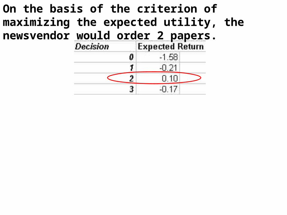
On the basis of the criterion of maximizing the expected utility, the newsvendor would order 2 papers.

Consider the following auto insurance example:Ten years after graduating from Standford’s Graduate School of Business, Carol Lane purchased a Lexus. The annual premium from her insurance company for collision insurance would be $1000 with $250 deductible. There is only a 0.5% chance she will cause a collision in the next year. In this case, she can expect about $50,000 worth of damage. Since she owns the Lexus outright, she is not required to purchase collision insurance. Should she buy the insurance or not?

=B2 + B1=B6

=B1

=SUMPRODUCT(E3:F3,$E$6:$F$6)

Here is the spreadsheet model:

The Expected Returns indicate that it would be less expensive for her, on average, to not buy the insurance.

Based on the expected utility analysis, Carol feels it is worth buying the insurance to have peace of mind that she won’t have to pay $50,000 if she causes a collision.

However, to be sure, she performs an utility analysis. She decides that she is risk-averse, and estimates her r value to be $10,000.

=1-EXP(E3/$F$8)

End of Part 1Please continue to Part 2