Decision Making Under Uncertainty: Capturing

Dynamic Brand Choice Processes in Turbulent

Consumer Goods Market.

Tulin Erdem and Michael Keane.

1

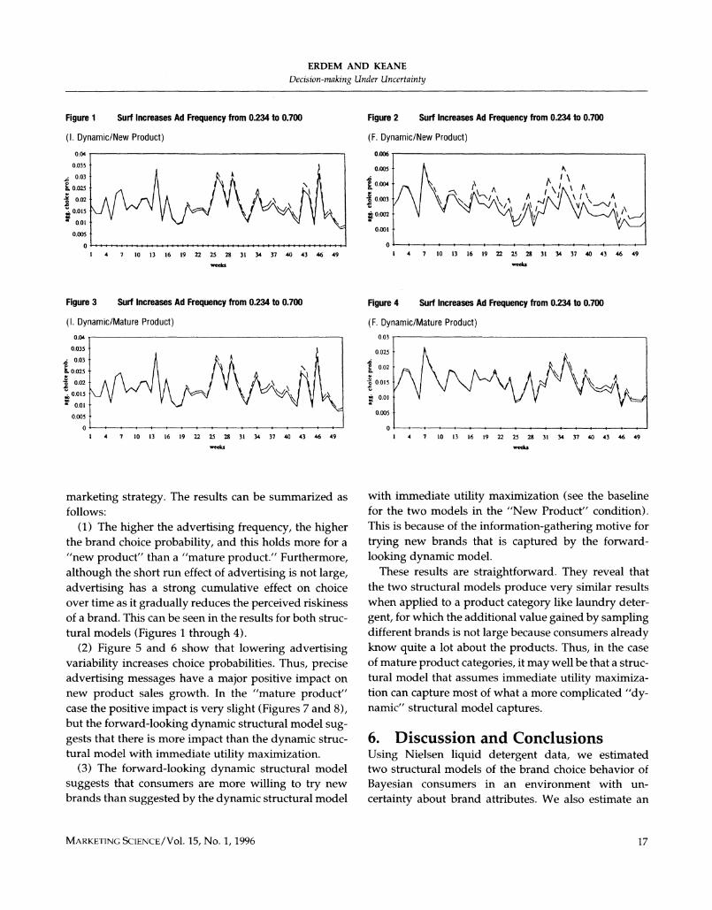
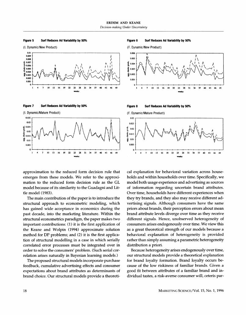
• In forward looking dynamic structural models, con-sumers may sample different brands exclusively togather information about them.

• After some sampling, consumers may settle into abrand.

• Changes, due to the introduction of new brands,brand repositioning, price cuts of other brands mayinduce consumers to resample.

• Structural models of consumer choice and learningfit the data better than the standard reduced formmodels.

2

• Obtain deeper understanding of the consumer learn-

ing process, which is the source of state depen-

dence. Policy experiments can be done.

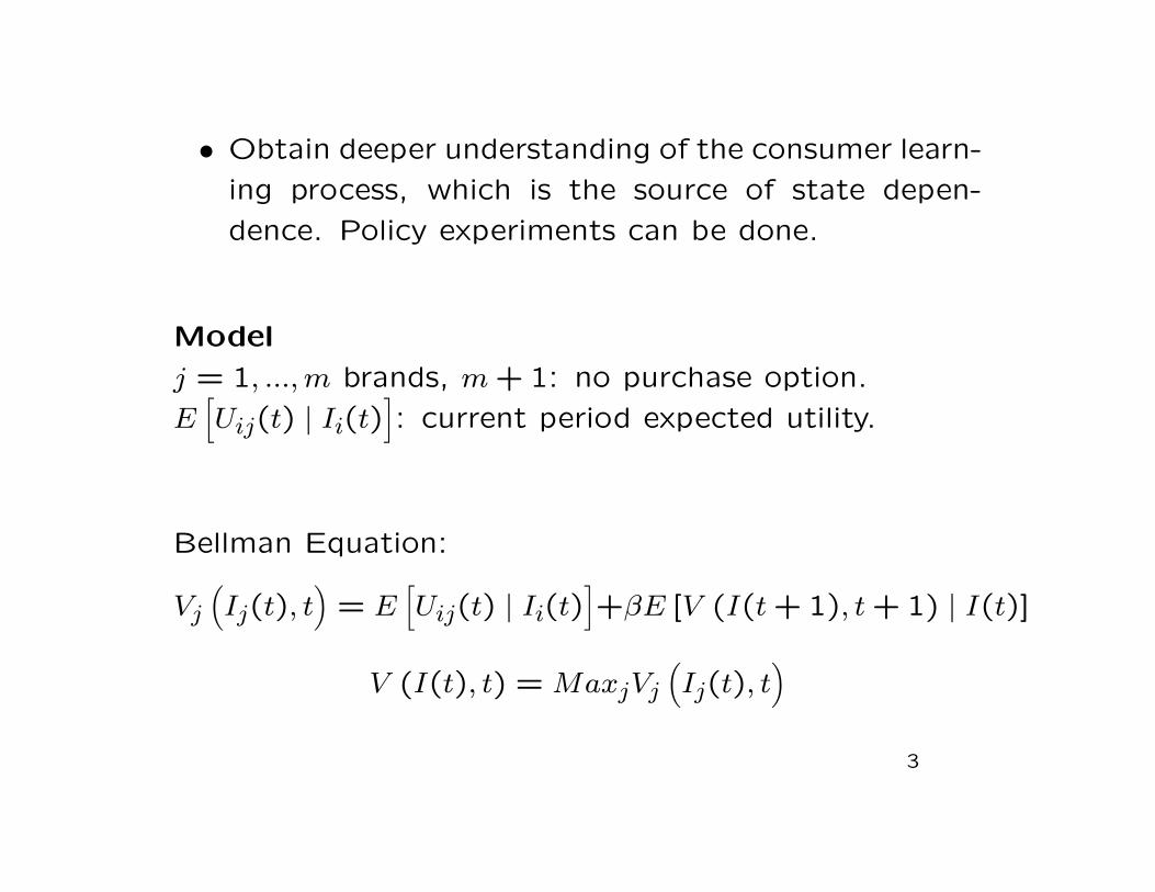
Model

j = 1, ...,m brands, m+ 1: no purchase option.

E[Uij(t) | Ii(t)

]: current period expected utility.

Bellman Equation:

Vj(Ij(t), t

)= E

[Uij(t) | Ii(t)

]+βE [V (I(t+ 1), t+ 1) | I(t)]

V (I(t), t) = MaxjVj(Ij(t), t

)3

Consumer Expected Utility

AEijt : consumer i’s experience of a brand’s attribute.

Utility of consumer i purchasing a brand j:

Uijt = −wjPijt + wAAEijt − wArA2Eijt + eijt

r: consumer risk component.

r > 0 risk averse

r = 0 risk neutral

r < 0 risk loving

4

E[Uijt | Ii(t)

]= −wjPijt + wAE

[AEijt | Ii(t)

]− wArE

[AEijt | Ii(t)

]2−wArE

[AEijt − E

[A2Eijt | Ii(t)

]]2+ eijt

r: consumer risk component.

Other small brands:

E [UiOt] = UiOt = ΦO + ΦOt + eiOt

No purchase option:

E [UiNPt] = UiNPt = ΦNP + ΦNPt + eiNPt

5

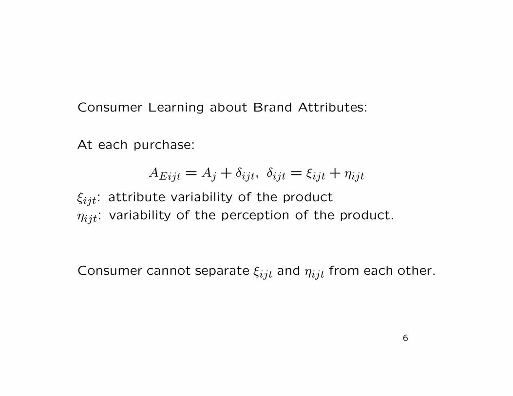
Consumer Learning about Brand Attributes:

At each purchase:

AEijt = Aj + δijt, δijt = ξijt + ηijt

ξijt: attribute variability of the product

ηijt: variability of the perception of the product.

Consumer cannot separate ξijt and ηijt from each other.

6

At the introduction of the brand (no past learning)

δijt ∼ N(0, σ2δ ), Aj ∼ N(A, σ2

A(0))

Advertising signal:

Sijt = Aj + ςijt, ςijt ∼ N(0, σ2ς )

Consumer update:

E[AEijt+1 | Ii(t)

]= E

[AEijt | Ii(t− 1)

]+D1ijtβ1ij(t)

[AEijt − E

[AEijt | Ii(t− 1)

]]+D2ijtβ2ij(t)

[SEijt − E

[SEjt | Ii(t− 1)

]]D1ijt: dummy of whether consumer purchases brand j

or not.D2ijt: dummy of whether consumer receives an adver-tising signal of brand j or not.

7

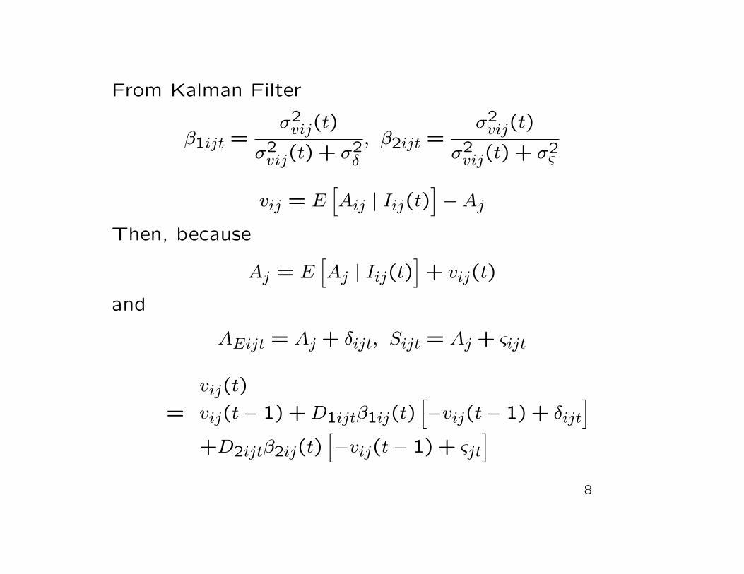
From Kalman Filter

β1ijt =σ2vij(t)

σ2vij(t) + σ2

δ

, β2ijt =σ2vij(t)

σ2vij(t) + σ2

ς

vij = E[Aij | Iij(t)

]−Aj

Then, because

Aj = E[Aj | Iij(t)

]+ vij(t)

and

AEijt = Aj + δijt, Sijt = Aj + ςijt

vij(t)

= vij(t− 1) +D1ijtβ1ij(t)[−vij(t− 1) + δijt

]+D2ijtβ2ij(t)

[−vij(t− 1) + ςjt

]8

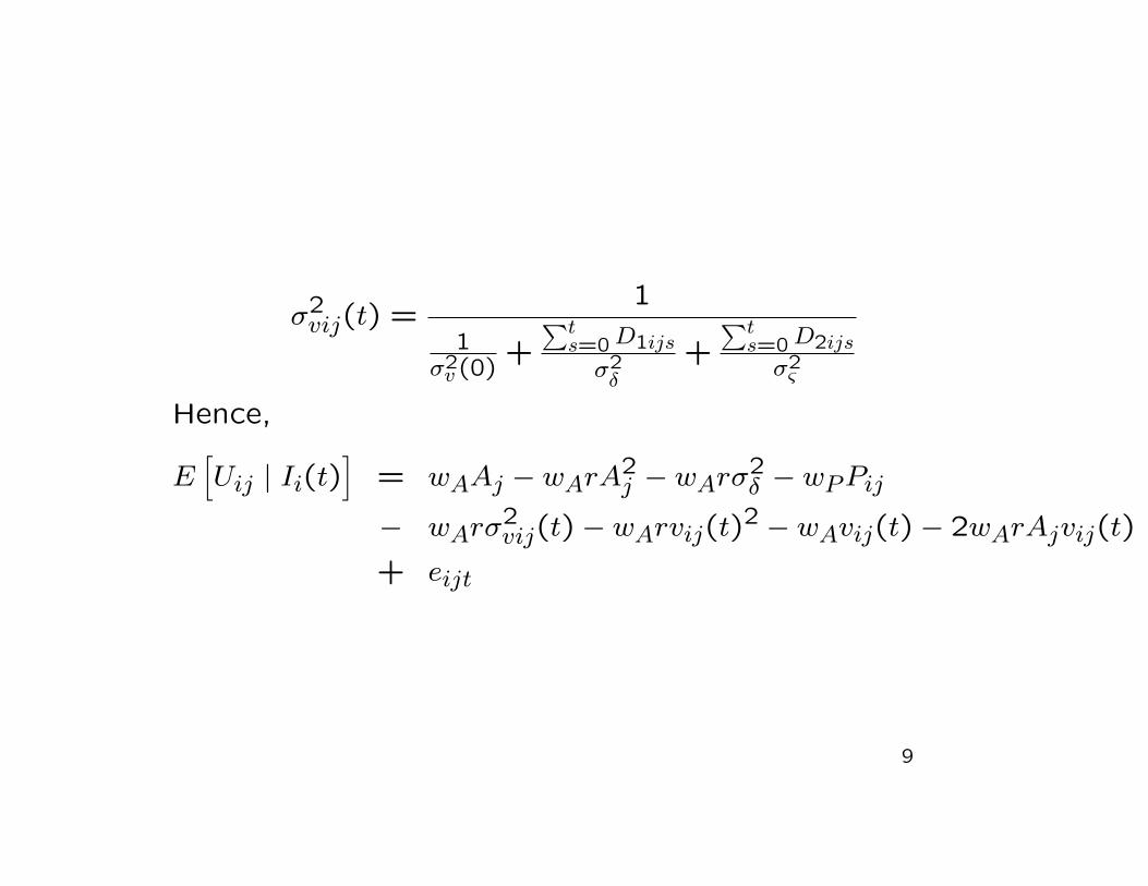
σ2vij(t) =

1

1σ2v (0)

+∑ts=0D1ijs

σ2δ

+∑ts=0D2ijs

σ2ς

Hence,

E[Uij | Ii(t)

]= wAAj − wArA2

j − wArσ2δ − wPPij

− wArσ2vij(t)− wArvij(t)

2 − wAvij(t)− 2wArAjvij(t)

+ eijt

9

Static brand choice probability:

Pi(Ii(t), t) =∫ exp

{E[Uij | Ii(t)

]}∑k exp {E [Uik | Ii(t)]}

f(v)dv

Dynamic brand choice probability:

Pi(Ii(t), t) =∫ exp

{E[Vij | Ii(t)

]}∑k exp {E [Vik | Ii(t)]}

f(v)dv

where

E[Vij | Ii(t)

]= E

[Uij | Ii(t)

]+βE

[Vij | Ii(t+ 1) | dijt = 1, Ii(t)

]

10

Data:

• Scanner panel data for laundry detergent, 3,000

households from year 1986 to 1988.

• New brands were introduced

• Firms heavily advertise

• Low in variety seeking.

• Only liquid detergents.

11

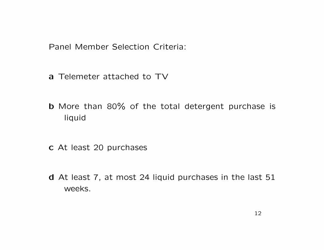
Panel Member Selection Criteria:

a Telemeter attached to TV

b More than 80% of the total detergent purchase is

liquid

c At least 20 purchases

d At least 7, at most 24 liquid purchases in the last 51

weeks.

12

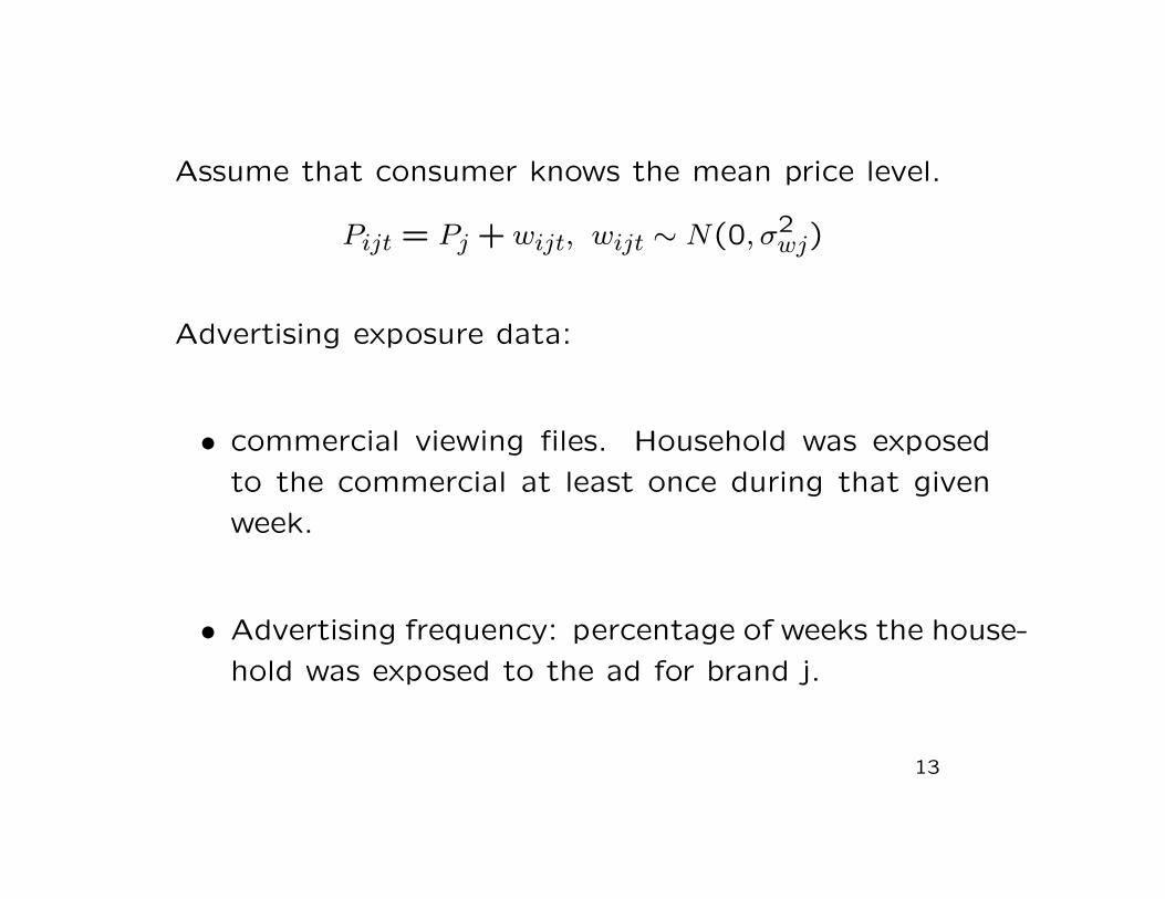
Assume that consumer knows the mean price level.

Pijt = Pj + wijt, wijt ∼ N(0, σ2wj)

Advertising exposure data:

• commercial viewing files. Household was exposed

to the commercial at least once during that given

week.

• Advertising frequency: percentage of weeks the house-

hold was exposed to the ad for brand j.

13

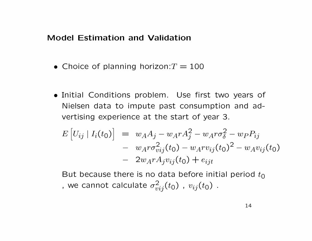
Model Estimation and Validation

• Choice of planning horizon:T = 100

• Initial Conditions problem. Use first two years of

Nielsen data to impute past consumption and ad-

vertising experience at the start of year 3.

E[Uij | Ii(t0)

]= wAAj − wArA2

j − wArσ2δ − wPPij

− wArσ2vij(t0)− wArvij(t0)2 − wAvij(t0)

− 2wArAjvij(t0) + eijt

But because there is no data before initial period t0, we cannot calculate σ2

vij(t0) , vij(t0) .

14

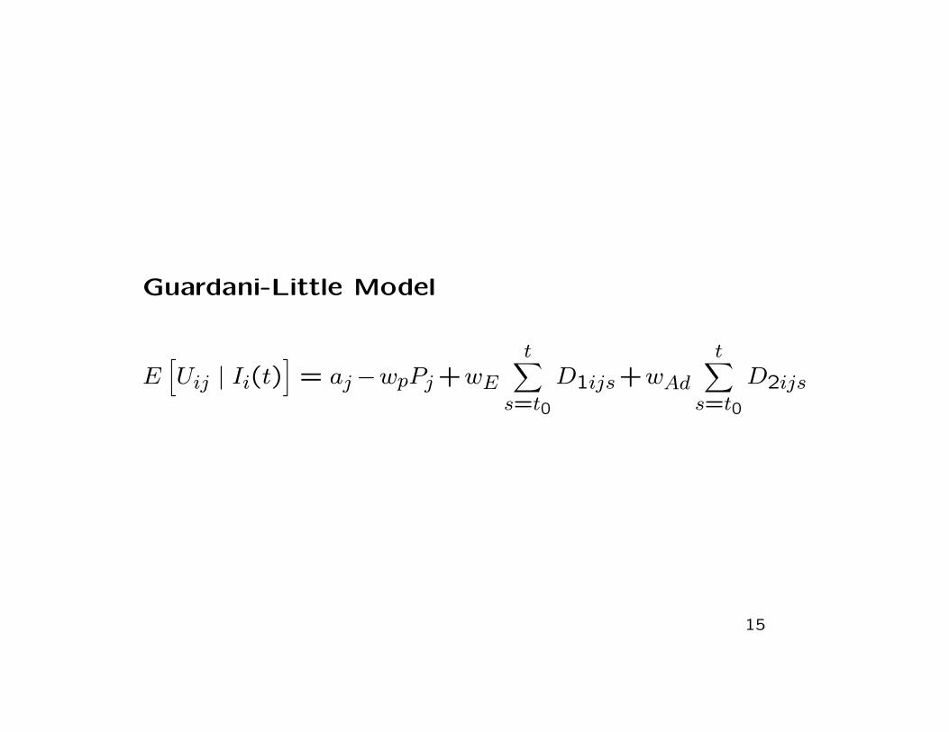
Guardani-Little Model

E[Uij | Ii(t)

]= aj−wpPj+wE

t∑s=t0

D1ijs+wAd

t∑s=t0

D2ijs

15

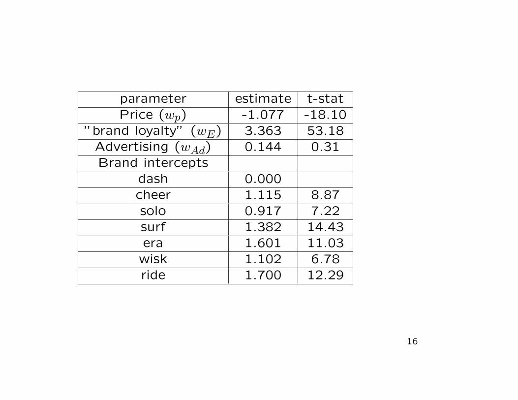
parameter estimate t-statPrice (wp) -1.077 -18.10

”brand loyalty” (wE) 3.363 53.18Advertising (wAd) 0.144 0.31Brand intercepts

dash 0.000cheer 1.115 8.87solo 0.917 7.22surf 1.382 14.43era 1.601 11.03

wisk 1.102 6.78ride 1.700 12.29

16

parameter estimate t-statOther brands intercept -0.633 -2.98

Other brands trend 0.011 4.87No purchase intercept 1.636 8.02

No purchase trend 0.005 1.35Brand loyalty smoothing 0.770 50.62Advertising smoothing 0.788 2.95

Advertising coefficient has positive sign but not signif-

icant.

Smoothing: total past purchases or advertising?

17

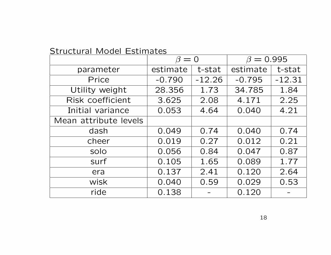
Structural Model Estimatesβ = 0 β = 0.995

parameter estimate t-stat estimate t-statPrice -0.790 -12.26 -0.795 -12.31

Utility weight 28.356 1.73 34.785 1.84Risk coefficient 3.625 2.08 4.171 2.25Initial variance 0.053 4.64 0.040 4.21

Mean attribute levelsdash 0.049 0.74 0.040 0.74cheer 0.019 0.27 0.012 0.21solo 0.056 0.84 0.047 0.87surf 0.105 1.65 0.089 1.77era 0.137 2.41 0.120 2.64

wisk 0.040 0.59 0.029 0.53ride 0.138 - 0.120 -

18

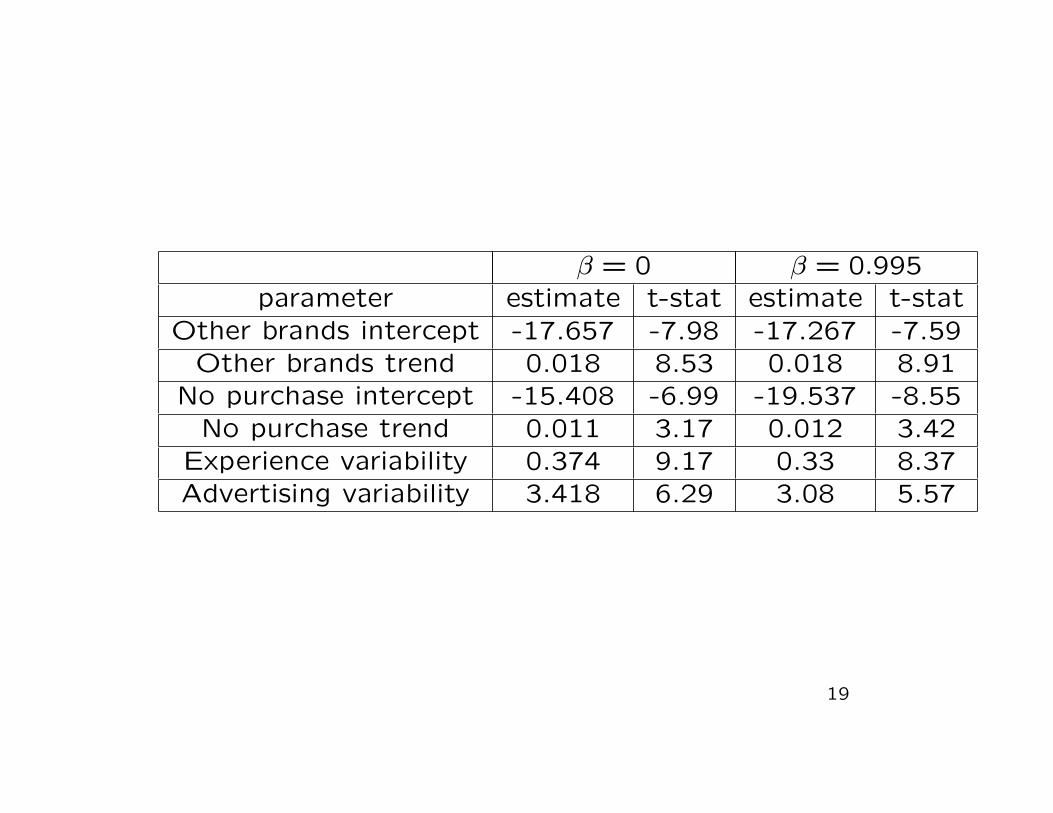
β = 0 β = 0.995parameter estimate t-stat estimate t-stat

Other brands intercept -17.657 -7.98 -17.267 -7.59Other brands trend 0.018 8.53 0.018 8.91

No purchase intercept -15.408 -6.99 -19.537 -8.55No purchase trend 0.011 3.17 0.012 3.42

Experience variability 0.374 9.17 0.33 8.37Advertising variability 3.418 6.29 3.08 5.57

19

• Fixed one attribute level (tide) to a value such that

the utility is increasing in the attribute level.

• Parameter estimates of the two models are similar.

• Price coefficients are negative and significant

• High utility weight on latent attribute: cleansing

power.

• Attribute levels are not significant, but the differ-

ences are.

20

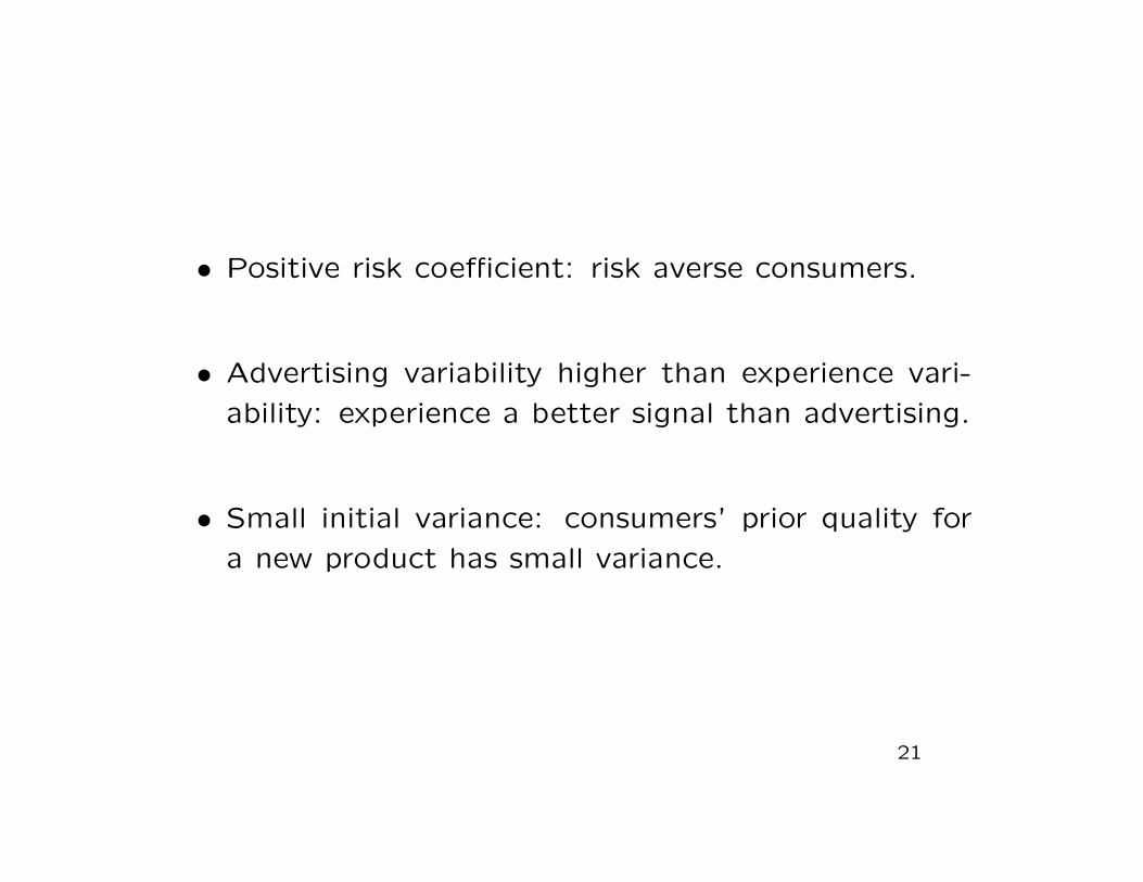
• Positive risk coefficient: risk averse consumers.

• Advertising variability higher than experience vari-

ability: experience a better signal than advertising.

• Small initial variance: consumers’ prior quality for

a new product has small variance.

21

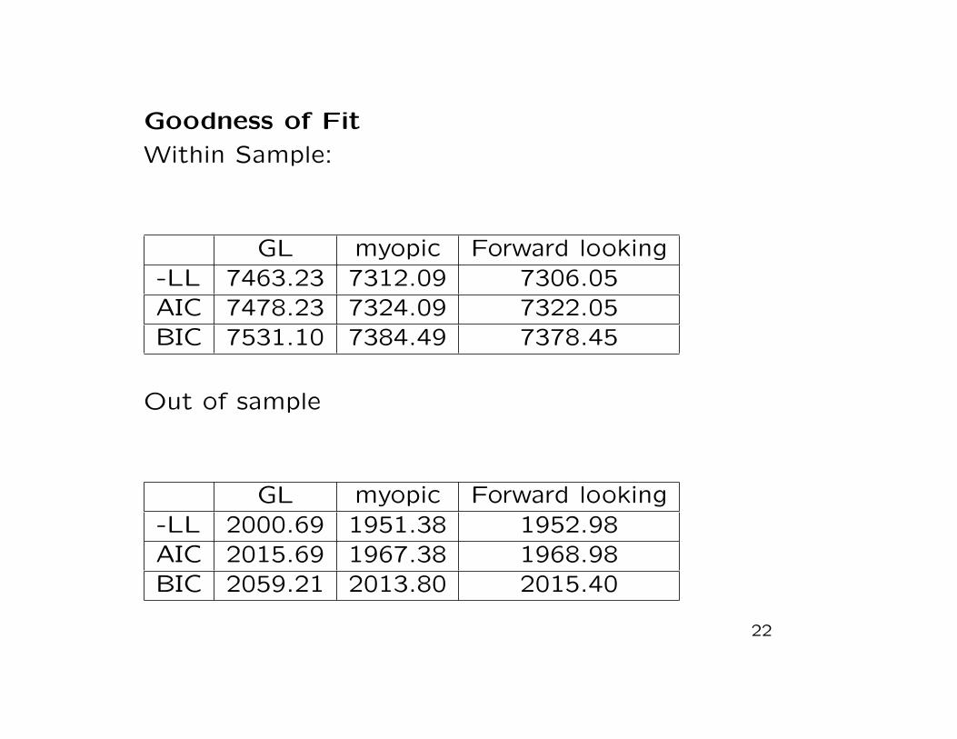
Goodness of Fit

Within Sample:

GL myopic Forward looking-LL 7463.23 7312.09 7306.05AIC 7478.23 7324.09 7322.05BIC 7531.10 7384.49 7378.45

Out of sample

GL myopic Forward looking-LL 2000.69 1951.38 1952.98AIC 2015.69 1967.38 1968.98BIC 2059.21 2013.80 2015.40

22