Decentralizing Corruption? Irrigation Reform in...

Motivation Context and data Estimation strategies Results Conclusions

Decentralizing Corruption? Irrigation Reform inPakistan’s Indus Basin

Freeha Fatima Hanan G. Jacoby Ghazala MansuriWorld Bank

ABCDEWashington DC

June 20-21, 2016


Centralization vs. Decentralization

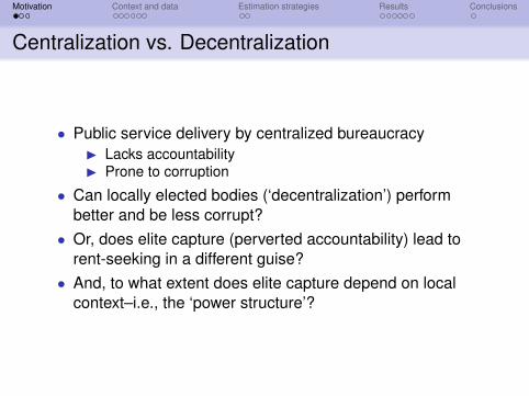
• Public service delivery by centralized bureaucracyI Lacks accountabilityI Prone to corruption

• Can locally elected bodies (‘decentralization’) performbetter and be less corrupt?• Or, does elite capture (perverted accountability) lead to

rent-seeking in a different guise?• And, to what extent does elite capture depend on local

context–i.e., the ‘power structure’?


Empirical Questions

• Decentralization empirics have been hampered byI Lack of objective measure of rent-seekingI Lack of large-scale ‘experiment’ in decentralization

• RCTs (Alatas et al. 2013, Beath et al. 2013)I Provide evidence on how elite capture varies with

(experimentally induced) institutions of local governmentI But not on the broader question of how local governance

compares to centralized bureaucracy.


Irrigation Reform Experiment in the Indus Basin

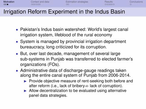
• Pakistan’s Indus basin watershed: World’s largest canalirrigation system, lifeblood of the rural economy• System is managed by provincial irrigation department

bureaucracy, long criticized for its corruption.• But, over last decade, management of several large

sub-systems in Punjab was transferred to elected farmer’sorganizations (FOs).• Administrative data of discharge-gauge readings taken

along the entire canal system of Punjab from 2006-2014.I Provide objective measure of rent-seeking both before and

after reform (i.e., lack of bribery; lack of corruption).I Allow decentralization to be evaluated using alternative

panel data strategies.


Status Quo Ante

• Each outlet along a channel supplies a watercourse alongwhich several dozen farmers take turns irrigating.• In theory, outlet dimensions are calculated to deliver a

specific discharge proportional to command area ofwatercourse.• In reality, farmers, especially those at the head of the

channel, illicitly enlarge their outlets or even break into thechannel itself to increase their water allocation. outlet tampering

• Typically, farmers bribe irrigation officials to avoid takingaction or prosecuting the offense.


The Reform

• Punjab irrigation system divided into 17 Circles, eachmeant to establish an Area Water Board (AWB).• Five AWBs initially sanctioned to form FOs (FO Circles);

reform subsequently stalled leaving 12 non-FO circles.• FOs tasked with maintaining channels, monitoring

rotational system to ensure equitable allocation, mediatingdisputes, and collecting water taxes.• Distributary-level FO is run by 9-member management

committee (MC) elected from among outlet-level chairmen.• MC tenure is 3 yrs. (again, in theory!) reform timeline


Canal Discharge Data

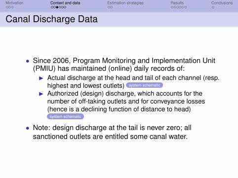
• Since 2006, Program Monitoring and Implementation Unit(PMIU) has maintained (online) daily records of:I Actual discharge at the head and tail of each channel (resp.

highest and lowest outlets) system schematic

I Authorized (design) discharge, which accounts for thenumber of off-taking outlets and for conveyance losses(hence is a declining function of distance to head)

system schematic

• Note: design discharge at the tail is never zero; allsanctioned outlets are entitled some canal water.


Metrics

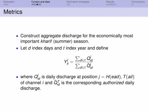
• Construct aggregate discharge for the economically mostimportant kharif (summer) season.• Let d index days and t index year and define

Y jit =

∑d∈t Qj

id∑d∈t Q̄j

id

• where Qjid is daily discharge at position j = H(ead),T (ail)

of channel i and Q̄Tid is the corresponding authorized daily

discharge.


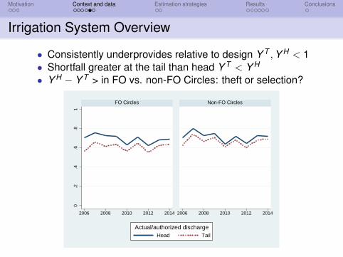
Irrigation System Overview

• Consistently underprovides relative to design Y T ,Y H < 1• Shortfall greater at the tail than head Y T < Y H

• Y H − Y T > in FO vs. non-FO Circles: theft or selection?0

.2.4

.6.8

1

2006 2008 2010 2012 2014 2006 2008 2010 2012 2014

FO Circles Non-FO Circles

Head TailActual/authorized discharge


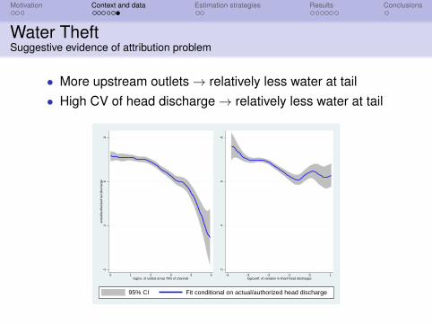
Water TheftSuggestive evidence of attribution problem

• More upstream outlets→ relatively less water at tail• High CV of head discharge→ relatively less water at tail

.2.4

.6.8

actu

al/a

utho

rized

tail

disc

harg

e

0 1 2 3 4 5log(no. of outlets at top 75% of channel)

.2.4

.6.8

-4 -3 -2 -1 0 1log(coeff. of variation in kharif head discharge)

95% CI Fit conditional on actual/authorized head discharge


Pipeline Strategy

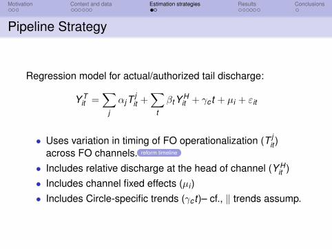
Regression model for actual/authorized tail discharge:

Y Tit =

∑j

αjTjit +

∑t

βtY Hit + γc t + µi + εit

• Uses variation in timing of FO operationalization (T jit )

across FO channels. reform timeline

• Includes relative discharge at the head of channel (Y Hit )

• Includes channel fixed effects (µi )• Includes Circle-specific trends (γc t)– cf., ‖ trends assump.


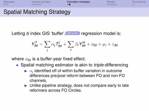
Spatial Matching Strategy

Letting b index GIS ‘buffer’, GIS buffer regression model is:

Y Tibt =

∑j

αjTjibt +

∑t

βtY Hibt + φbt + µi + εibt

where φbt is a buffer-year fixed effect.• Spatial matching estimator is akin to triple-differencing

I αj identified off of within buffer variation in outcomedifferences pre/post reform between FO and non-FOchannels.

I Unlike pipeline strategy, does not compare early to latereformers across FO Circles.


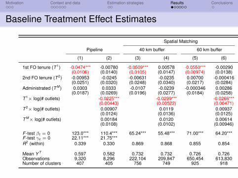
Baseline Treatment Effect Estimates

Spatial Matching

Pipeline 40 km buffer 60 km buffer

(1) (2) (3) (4) (5) (6)

1st FO tenure (T 1) -0.0474*** -0.00780 -0.0509*** 0.00578 -0.0550*** -0.00290(0.0106) (0.0140) (0.0105) (0.0147) (0.00974) (0.0138)

2nd FO tenure (T 2) -0.00953 -0.0245 -0.00631 -0.0235 0.00700 -0.000416(0.0251) (0.0320) (0.0248) (0.0340) (0.0217) (0.0284)

Administrated (T M ) 0.0303 0.0333 -0.0107 -0.0239 -0.000346 0.00286(0.0187) (0.0269) (0.0196) (0.0277) (0.0184) (0.0258)

T 1× log(# outlets) -0.0225*** -0.0299*** -0.0266***(0.00443) (0.00522) (0.00471)

T 2× log(# outlets) 0.00907 0.0119 0.00937(0.0124) (0.0136) (0.0125)

T M× log(# outlets) 0.00184 0.0120 0.00614(0.0108) (0.0102) (0.00946)

F -test βt = 0 123.0*** 110.4*** 65.24*** 55.48*** 71.00*** 64.20***F -test γc = 0 22.11*** 21.75***R2 (within) 0.339 0.330 0.869 0.868 0.855 0.854

Mean Y T 0.597 0.582 0.732 0.732 0.726 0.726Observations 9,320 8,296 222,104 209,847 650,454 613,830Number of clusters 407 405 756 749 925 918


Accountability of FOs

• Summary: Water theft increases after canal managementis transferred from Irrigation Dept. to FOs (in first tenure).• ⇒ Rent-seeking is more restrained under bureaucracy

than under local governance (perhaps bureaucrats havecareer concerns and thus cannot be too profligate).• Are some FOs more accountable to tail-enders than

others?I Narrowly: consider variation in tail representation on MCI Broadly: consider variation in land inequality along channel


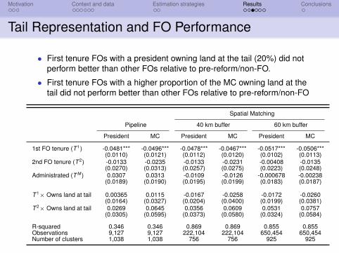
Tail Representation and FO Performance

• First tenure FOs with a president owning land at the tail (20%) did notperform better than other FOs relative to pre-reform/non-FO.

• First tenure FOs with a higher proportion of the MC owning land at thetail did not perform better than other FOs relative to pre-reform/non-FO

Spatial Matching

Pipeline 40 km buffer 60 km buffer

President MC President MC President MC

1st FO tenure (T 1) -0.0481*** -0.0496*** -0.0478*** -0.0467*** -0.0517*** -0.0506***(0.0110) (0.0121) (0.0112) (0.0120) (0.0102) (0.0113)

2nd FO tenure (T 2) -0.0133 -0.0235 -0.0133 -0.0231 -0.00408 -0.0135(0.0270) (0.0313) (0.0257) (0.0275) (0.0223) (0.0248)

Administrated (T M ) 0.0307 0.0313 -0.0109 -0.0126 -0.000678 -0.00238(0.0189) (0.0190) (0.0195) (0.0199) (0.0183) (0.0187)

T 1× Owns land at tail 0.00365 0.0115 -0.0167 -0.0258 -0.0172 -0.0260(0.0164) (0.0327) (0.0204) (0.0400) (0.0199) (0.0381)

T 2× Owns land at tail 0.0269 0.0645 0.0356 0.0609 0.0531 0.0757(0.0305) (0.0595) (0.0373) (0.0580) (0.0324) (0.0584)

R-squared 0.346 0.346 0.869 0.869 0.855 0.855Observations 9,127 9,127 222,104 222,104 650,454 650,454Number of clusters 1,038 1,038 756 756 925 925


Power Structure

• FOs perform equally poorly whether or not they nominallyrepresent tail-enders⇒‘voice’ is window dressing.• Is there a deeper determinant of FO performance?• Literature (e.g., Mansuri and Rao, 2013) suggests that

where inequality is higher, local government is more likelyto serve interests of wealthy and powerful.• How to measure inequality in this setting?

I Of what asset? Land (available in Ag. censuses)I Over what population? {Cultivators} ∪ {Landowners}I With what statistic? Top shares (to get at concentration)


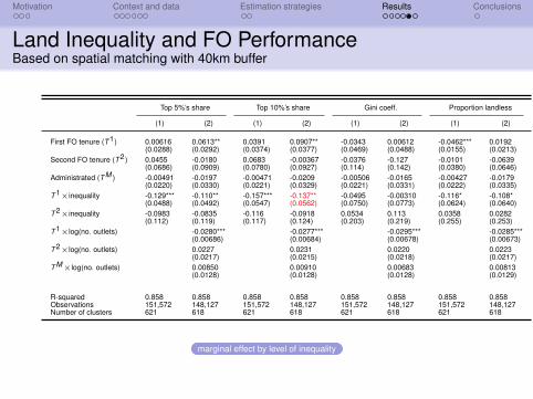
Land Inequality and FO PerformanceBased on spatial matching with 40km buffer

Top 5%’s share Top 10%’s share Gini coeff. Proportion landless

(1) (2) (1) (2) (1) (2) (1) (2)

First FO tenure (T 1) 0.00616 0.0613** 0.0391 0.0907** -0.0343 0.00612 -0.0462*** 0.0192(0.0288) (0.0292) (0.0374) (0.0377) (0.0469) (0.0488) (0.0155) (0.0213)

Second FO tenure (T2) 0.0455 -0.0180 0.0683 -0.00367 -0.0376 -0.127 -0.0101 -0.0639(0.0686) (0.0909) (0.0780) (0.0927) (0.114) (0.142) (0.0380) (0.0646)

Administrated (T M ) -0.00491 -0.0197 -0.00471 -0.0209 -0.00506 -0.0165 -0.00427 -0.0179(0.0220) (0.0330) (0.0221) (0.0329) (0.0221) (0.0331) (0.0222) (0.0335)

T 1×inequality -0.129*** -0.110** -0.157*** -0.137** -0.0495 -0.00310 -0.116* -0.108*(0.0488) (0.0492) (0.0547) (0.0562) (0.0750) (0.0773) (0.0624) (0.0640)

T 2×inequality -0.0983 -0.0835 -0.116 -0.0918 0.0534 0.113 0.0358 0.0282(0.112) (0.119) (0.117) (0.124) (0.203) (0.219) (0.255) (0.253)

T 1×log(no. outlets) -0.0280*** -0.0277*** -0.0295*** -0.0285***(0.00686) (0.00684) (0.00678) (0.00673)

T 2×log(no. outlets) 0.0227 0.0231 0.0220 0.0223(0.0217) (0.0215) (0.0218) (0.0217)

T M×log(no. outlets) 0.00850 0.00910 0.00683 0.00813(0.0128) (0.0128) (0.0128) (0.0129)

R-squared 0.858 0.858 0.858 0.858 0.858 0.858 0.858 0.858Observations 151,572 148,127 151,572 148,127 151,572 148,127 151,572 148,127Number of clusters 621 618 621 618 621 618 621 618

marginal effect by level of inequality


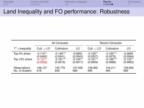
Land Inequality and FO performance: Robustness

All Censuses Recent Censuses

T 1×inequality Cult. ∪ LO Cultivators LO Cult. ∪ LO Cultivators LO

Top 5% share -0.110** -0.148*** -0.0855 -0.126** -0.165*** -0.0909(0.0492) (0.0541) (0.0543) (0.0527) (0.0579) (0.0564)

Top 10% share -0.137** -0.181*** -0.130** -0.161** -0.195*** -0.132**(0.0562) (0.0619) (0.0617) (0.0626) (0.0686) (0.0662)

Observations 148,127 145,778 137,006 139,365 134,211 129,856No. of clusters 618 609 588 595 584 569


Summary and Implications

• Transferring canal management from irrigation departmentbureaucrats to FOs increased water theft⇒ elite captureis a real concern (contra Atalas et al. 2013).• Indeed, local institutions perform worse precisely where

there are strong elites (i.e., concentrated landholdings).• While decentralization in the Indus basin did not deliver on

its promise of a more equitable canal water distribution, itmay be premature to entirely foresake irrigation reform.• Designing representative institutions that mitigate elite

capture could tip the balance in favor of local control.

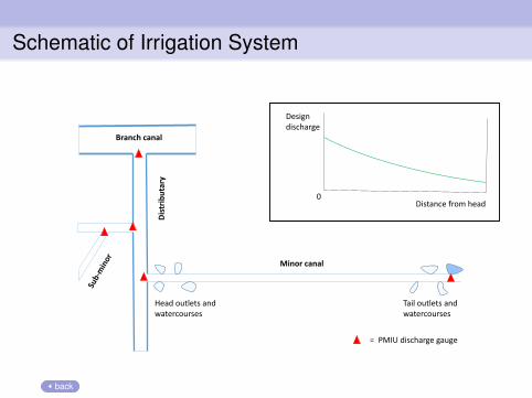
Schematic of Irrigation System

Head outlets and watercourses

Tail outlets and watercourses

Dis

trib

uta

ry

Minor canal

Design discharge

Distance from head0

= PMIU discharge gauge

Branch canal

back

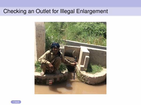
Checking an Outlet for Illegal Enlargement

back

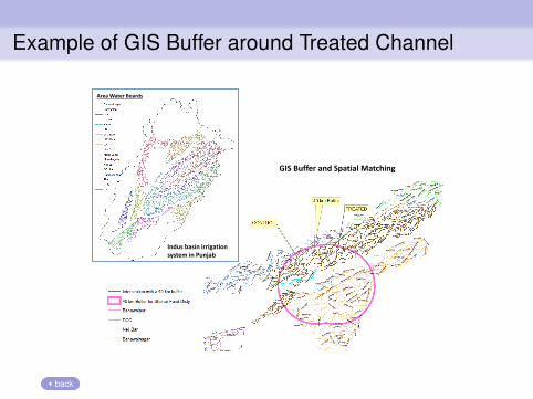
Example of GIS Buffer around Treated Channel

Area Water Boards

Indus basin irrigation system in Punjab

GIS Buffer and Spatial Matching

back

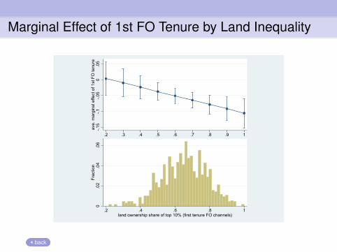
Marginal Effect of 1st FO Tenure by Land Inequality

-.15

-.1-.0

50

.05

ave.

mar

gina

l effe

ct o

f 1st

FO

tenu

re

.2 .3 .4 .5 .6 .7 .8 .9 1

0.0

2.0

4.0

6Fr

actio

n

.2 .4 .6 .8 1land ownership share of top 10% (first tenure FO channels)

back

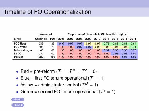
Timeline of FO Operationalization

Number of Proportion of channels in Circle within regime

Circle Channels FOs 2006 2007 2008 2009 2010 2011 2012 2013 2014

LCC East 235 85 0.97 0.97 0.97 0.97 0.97 0.73 0.85 0.86 0.91LCC West 198 73 1.00 1.00 0.97 0.97 0.98 0.98 0.98 0.98 0.74Bahawalnagar 146 69 1.00 1.00 1.00 1.00 1.00 0.97 0.97 0.97 0.57LBDC 237 60 1.00 1.00 1.00 1.00 1.00 1.00 0.98 0.98 1.00Derajat 222 120 1.00 1.00 1.00 1.00 1.00 1.00 1.00 1.00 1.00

• Red = pre-reform (T 1 = T M = T 2 = 0)• Blue = first FO tenure operational (T 1 = 1)• Yellow = administrator control (T M = 1)• Green = second FO tenure operational (T 2 = 1)

back 1

back 2

Decentralizing Corruption? Irrigation Reform in...

Documents

Transcript of Decentralizing Corruption? Irrigation Reform in...