Debt Overhang, Monetary Policy, and EconomicRecoveries After Large Recessions∗

Christian Bustamante†

Bank of Canada

First version: November 1, 2018This version: February 13, 2020

Abstract

This paper explores why conventional monetary policy was insufficient in mitigating the severityof the 2007 U.S. recession and unsuccessful thereafter in stimulating the economic recovery. Usinga quantitative model alongside firm-level data, I show that accounting for individual firms’ debtstructures is crucial in explaining why business investment fell so dramatically through the recessionand remained low for several years despite the Federal Reserve repeatedly cutting its target interestrate until conventional policy tools were exhausted. Using a sample of publicly traded firms, Iestablish that firms with greater long-term debt exposure experienced larger contractions and slowerrecoveries in their investment. Next, I show that debt overhang episodes were unusually prevalentand doubled in severity over the years following the onset of the recession, and particularly so amongfirms relying more heavily on long-maturing debt.

I develop a New Keynesian model where heterogeneous firms finance investment using default-able long-term nominal debt, and a central bank faces an explicit zero lower bound constraint onthe short-term nominal interest rate, to understand these microeconomic observations and their im-plications for aggregate fluctuations. In the model, the greater a firm’s leverage, the higher its like-lihood of experiencing a debt overhang episode following a large aggregate shock. The incidenceof debt overhang episodes reduces investment in 6 percentage points in the stationary equilibriumand contributes by itself an additional 3.5 percentage points in further slowing the pace at whichinvestment recovers following a financial shock that resembles the Great Recession. Furthermore,these debt overhang problems compound with (1) debt deflation, and (2) the monetary authority’sinability to restore inflation once nominal interest rates reach the zero lower bound. Together, firms’long-maturity debt positions and the binding zero lower bound are critical in transmitting the conse-quences of a deep recession into a remarkably anemic recovery in aggregate investment.

Keywords: debt overhang, firm investment, long-term debt, monetary policy, ZLB.JEL Codes: E22, E32, E52.

∗I am extremely grateful to Julia Thomas and Aubhik Khan for guidance and support. I am also indebted toKyle Dempsey for his many insights and suggestions. I thank Manuel Amador, Ariel Burnstein, Anmol Bhandari,Nicolas Crouzet, Martin Eichenbaum, Nobu Kiyotaki, Indrajit Mitra, Venky Venkateswaran, and Michael Waugh,as well as Vanessa Ordoñez for helpful comments and suggestions.†E-mail: mail@cbustamante.co. Website: http://cbustamante.co. The views expressed in this paper are my

own and do not necessarily reflect the official views of the Bank of Canada.

1

1 Introduction

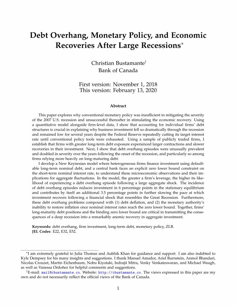
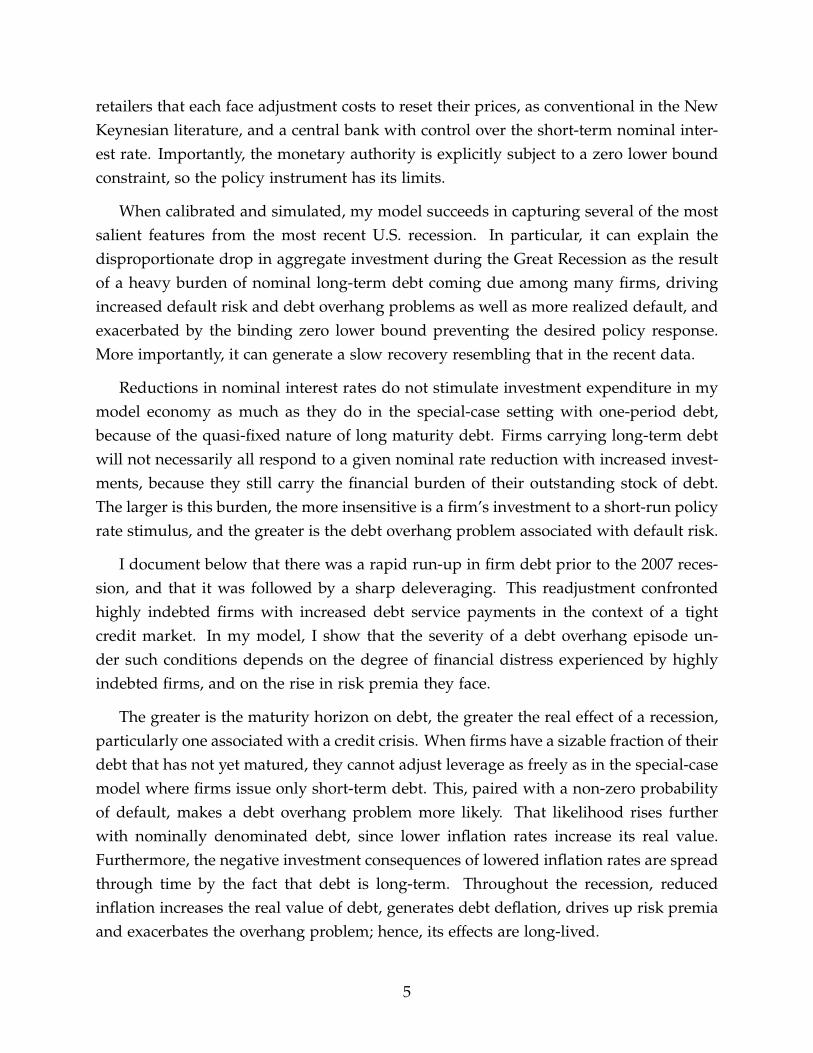
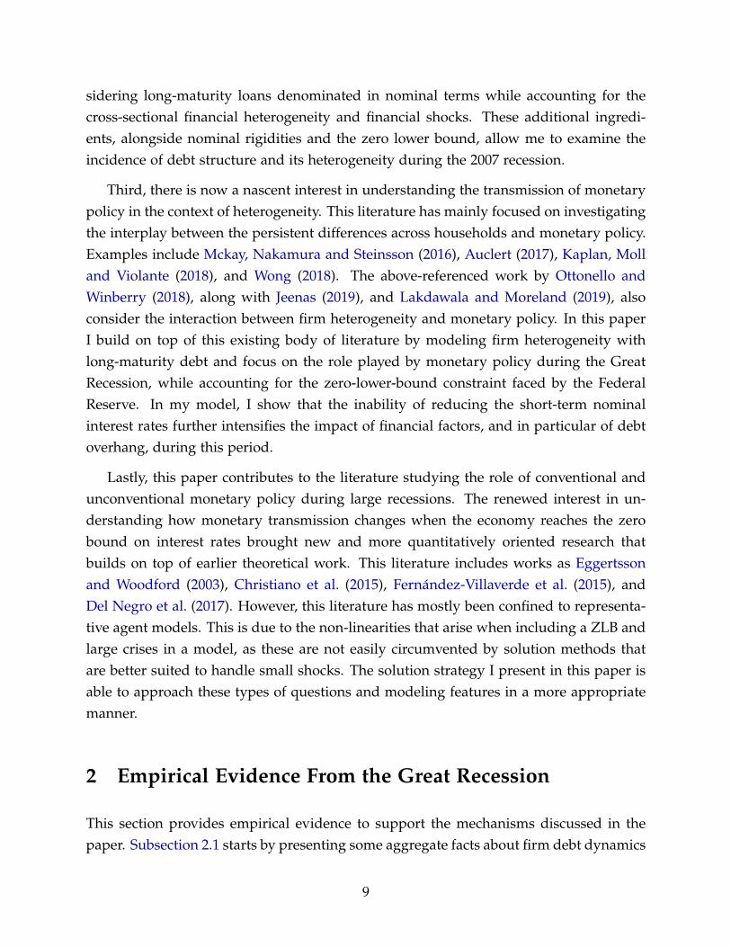
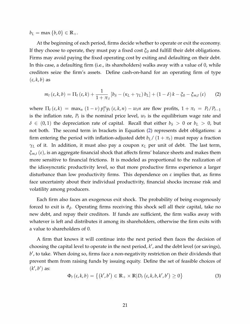
The U.S. economy experienced historically severe drops in firm investment during theGreat Recession, and these large declines persisted over several years. Figure 1(a) dis-plays detrended GDP, consumption, private investment, and business investment, re-porting each series as deviations relative to 2007Q4 levels. In the first two years of thecrisis, private investment and business investment experienced contractions of around20 percent. More importantly, investment recovered very slowly in the aftermath ofthe recession; four years after the onset of the financial crisis, private investment andbusiness investment were still well below their pre-crisis levels, by 7.5 and 9.9 percent,respectively. A similar pattern appears when we measure these series as shares of GDP(Figure 1(b)). This evidence suggests that residential investment was not alone in drivingthe unusual depth and persistence of the 2007 recession, but that firm investment alsocontributed significantly.

The Federal Reserve responded to the downturn with a sequence of rapid reductionsin nominal interest rates, taking the short-term policy rate from 5.25 percent in July 2007to almost zero by December 2008. Thereafter, on reaching the zero-lower bound, theFederal Reserve resorted to unconventional policy measures aimed at increasing liquid-ity in interbank markets, in an effort to fuel the credit supply and stimulate aggregateconsumption and investment (see Bernanke, 2012). Despite these strong policy interven-tions, investment recovered uncharacteristically gradually by comparison to the norm ofprevious postwar recessions.

This paper shows, both empirically and in the context of a quantitative general equi-librium model, that the interaction between heterogeneous firms’ long-term debt posi-tions and the monetary policy ramifications of the zero lower bound is crucial to under-standing the persistent dynamics of investment during a large recession and in its after-math. Long-term debt financing is prevalent in both the corporate and non-corporatesectors in the U.S., allowing firms a flexible means of smoothing their costs of invest-ment over time. This type of external finance leaves firms more exposed to rolloverrisk, however, and makes rapid adjustments in their debt positions difficult given ac-cumulated stocks. In such times of financial distress, firm investment activities maysuffer. A second, debt overhang, channel associated with firm ownership and defaultrisk compounds the problem. A firm is said to experience debt overhang when it hasthe opportunity to engage in positive net present value investment projects that wouldraise its expected value, but it decides not to undertake them due to balance sheet con-

2

Figure 1: The Great Recession

(a) Detrended Components of GDP

07-Q4 08-Q2 08-Q4 09-Q2 09-Q4 10-Q2 10-Q4 11-Q2 11-Q4

Date

-25

-20

-15

-10

-5

0

Percentagedev.from

2007Q4(detrended)

GDPConsumptionPrivate investmentBusiness investment

(b) Investment as Share of GDP

07-Q4 08-Q2 08-Q4 09-Q2 09-Q4 10-Q2 10-Q4 11-Q2 11-Q4

Date

-4

-3

-2

-1

0

Per

cent

poin

tsdev

.from

2007Q

4

Share private investmentShare business investment

Notes: Data from the U.S. Bureau of Economic Analysis, retrieved from FRED - St. LouisFed. Consumption is non-durable goods and services; business investment is non-residentialinvestment; and private investment is business fixed investment, residential investment, andconsumer durables. In panel (a), the log of each variable is detrended using an HP filter withweight 1600 and with data from 1947Q1 to 2017Q4. These series are plotted as percent devi-ations from their 2007Q4 values. Panel (b) reports the absolute percentage point deviationsin GDP shares with respect to the shares in 2007Q4.

siderations (Myers, 1977). During a debt overhang episode, investment decisions aredistorted, and firms choose sub-optimally low levels of capital. These episodes tendto occur in firms that are highly indebted and facing default risk, because cash flowsaccrue first to creditors in the event of default, not to shareholders. This misalignmentof incentives makes new investment projects less attractive for firms’ owners, loweringtheir investment rates.

Rollover risk and debt overhang arising from firms’ long-term debt positions werelarge impediments to investment activity during the Great Recession, because this reces-sion coincided with a severe contraction in the supply of credit to which firms could notrapidly re-accommodate. The consequences were particularly severe and long-lasting,because the zero lower bound prevented monetary policy from pushing inflation up,which otherwise would have eased the financial burden of affected firms. This conflatedthe problems posed by the stickiness in debt structures, setting the scene for a longanemic recovery in aggregate investment.

I evaluate the interaction and relative contribution of these channels in driving a slug-gish economic recovery, following a deep recession, in three ways. First, I examine andquantify the role of financial factors in explaining the slow aggregate investment recov-

3

ery over the post-2009Q2 U.S by means of an empirical analysis that uses firm-level datafrom Compustat. Second, I empirically establish that the effect of previously contractedlong-term financing on firm investment is more prevalent during large recessions. Third,I explore the extent to which monetary policy interacts with these financial factors in theface of a zero lower bound on nominal interest rates. To do so, I construct a generalequilibrium New Keynesian model with the essential ingredients necessary to explorethe extent to which the factors listed above explain what we observed during the reces-sion. There, I include a distribution of firms that vary in their need for external finance.These firms issue nominal long-term debt to finance their investment activities subjectto competitive lending terms responsive to their individual productivity, leverage, anddefault risk. Alongside them, there is a monetary authority confined by a zero lowerbound restriction.

My empirical results show a heterogeneous response in firm investment during theGreat Recession. Using firm-level data from Compustat, I first provide evidence thatlong-term debt is an important influence on firm investment decisions, and next doc-ument its prevalence at the onset of the 2007 crisis. My main empirical findings areas follow. First, firms with higher fractions of long-term debt maturing at the onsetof the recession experienced larger contractions in investment. Second, controlling forfirm-level variables highly correlated with investment choices does not eliminate the re-lationship; a large fraction of debt requiring rollover still predicts a strong decline inthe investment rate. Third, leverage does not completely summarize the relevance of afirm’s debt position as a determinant of investment, as it does not capture the timing atwhich that debt matures. Fourth, during the Great Recession, the adverse incidence oflong-term debt exposure doubled not only relative to normal times, but also relative toother crisis episodes.

As mentioned above, I conduct my theoretical investigation using a general equilib-rium New Keynesian model generalized to include defaultable long-term nominal debtand the investment and finance decisions among a rich distribution of firms. Firms facepersistent idiosyncratic productivity risk and are heterogeneous in their capital stocksand outstanding debt or financial savings. They produce a homogeneous good usingtheir own capital stocks together with labor they hire from a representative household.When their investment needs exceed their available cash, firms can finance the additionalexpenditure externally by issuing a defaultable nominal long-term bond purchased by aperfectly competitive financial intermediary. Alongside these distinctive new elementsin the model, I embed a Phillips curve by including a set of monopolistically competitive

4

retailers that each face adjustment costs to reset their prices, as conventional in the NewKeynesian literature, and a central bank with control over the short-term nominal inter-est rate. Importantly, the monetary authority is explicitly subject to a zero lower boundconstraint, so the policy instrument has its limits.

When calibrated and simulated, my model succeeds in capturing several of the mostsalient features from the most recent U.S. recession. In particular, it can explain thedisproportionate drop in aggregate investment during the Great Recession as the resultof a heavy burden of nominal long-term debt coming due among many firms, drivingincreased default risk and debt overhang problems as well as more realized default, andexacerbated by the binding zero lower bound preventing the desired policy response.More importantly, it can generate a slow recovery resembling that in the recent data.

Reductions in nominal interest rates do not stimulate investment expenditure in mymodel economy as much as they do in the special-case setting with one-period debt,because of the quasi-fixed nature of long maturity debt. Firms carrying long-term debtwill not necessarily all respond to a given nominal rate reduction with increased invest-ments, because they still carry the financial burden of their outstanding stock of debt.The larger is this burden, the more insensitive is a firm’s investment to a short-run policyrate stimulus, and the greater is the debt overhang problem associated with default risk.

I document below that there was a rapid run-up in firm debt prior to the 2007 reces-sion, and that it was followed by a sharp deleveraging. This readjustment confrontedhighly indebted firms with increased debt service payments in the context of a tightcredit market. In my model, I show that the severity of a debt overhang episode un-der such conditions depends on the degree of financial distress experienced by highlyindebted firms, and on the rise in risk premia they face.

The greater is the maturity horizon on debt, the greater the real effect of a recession,particularly one associated with a credit crisis. When firms have a sizable fraction of theirdebt that has not yet matured, they cannot adjust leverage as freely as in the special-casemodel where firms issue only short-term debt. This, paired with a non-zero probabilityof default, makes a debt overhang problem more likely. That likelihood rises furtherwith nominally denominated debt, since lower inflation rates increase its real value.Furthermore, the negative investment consequences of lowered inflation rates are spreadthrough time by the fact that debt is long-term. Throughout the recession, reducedinflation increases the real value of debt, generates debt deflation, drives up risk premiaand exacerbates the overhang problem; hence, its effects are long-lived.

5

My extension of the traditional New Keynesian model to interact a rich distribution offirms with long-term financing arrangements delivers interesting asymmetries and state-dependent responses of investment to monetary policy interventions. These nonlineardynamics in firm investment are a novel aspect of this paper and offer a few key insights.At the onset of a recession, we typically observe rising default rates. Firms issuingnew debt at such times face higher risk premia, which makes them more susceptible toexperiencing large distortions in their investment decisions due to debt overhang. Thisis especially true in times of large negative aggregate shocks and the recovery episodesthereafter. In those times, we observe sharp declines in aggregate investment that persist,because firms that are more prone to debt overhang problems are medium-sized firmswith growth opportunities and large fractions of long-term debt. By contrast, financialfrictions have more muted effects on investment in times of relatively small negativeshocks to the economy as these shocks do not raise default probabilities to the sameextent that large negative shocks do.

I find that the presence of debt finance with maturity structures resembling thosein the data matters particularly for macroeconomic fluctuations over large recessionsthat are financial in nature. The average maturity of debt is five years in my calibratedbaseline economy. There, a financial shock causes a recession with a recovery that isthree times the half-life than in a setting with one-year expected debt maturity. This isin part due to the persistent consequences of sharper rises in exit rates, and in part dueto a persistently greater worsening in the allocation of capital among incumbent firms.Each of these stems from a larger and more protracted increase in default risk underlonger maturity financing, which in turn generates a greater debt overhang burden.Moreover, by comparing the investment decisions of the firms in my model (equity-maximizing) with the ones of total-value-maximizing firms, I show that debt overhangproblems reduce aggregate investment in roughly 6 percentage points in the stationaryequilibrium. More importantly, following a negative financial shock, debt overhangfurther lowers aggregate investment in an additional 3.5 percentage points.

My model furthermore predicts that a debt deflation amplifies the effect of a financialshock, both in amplitude and persistence. Output falls an extra 1.5 percentage points andthe recovery is even more gradual when lower than expected inflation rates accompany afinancial recession. When considering changes in prices and interest rates, debt maturitydoes not have such a large impact on the size of the recession, but it still generates a morepersistent recovery. The half-life of the recovery is between two and three times largerin the five-year maturity model when compared to a two-year expected maturity case.

6

While the non-government channels discussed above go some distance toward ex-plaining the movements in aggregate business investment during and after the GreatRecession, I find that monetary policy still plays a critical and complementary role. Aswith the U.S. Federal Reserve, the central bank in my model economy is powerless togenerate inflationary pressures when it reaches the zero lower bound on nominal inter-est rates. This intensifies the debt deflation mechanism and exacerbates the overhangproblem, making it both more severe and more persistent. It is the combination of theseelements, the effective removal of the central bank’s policy instrument together withthe balance sheet factors raised above, that allows my model to explain a sizable por-tion of the sharp declines in U.S. investment during the 2007 U.S. recession and, moreimportantly, the confounding sluggishness in its recovery over four years beyond.

The rest of the paper is structured as follows. Section 2 describes the data andpresents suggestive evidence about the role of long-term financing during the 2007 crisis.Section 3 presents the model economy and discusses its primary mechanisms. Section 4and Section 5 describe the calibration and discuss the role of default risk and debt over-hang in the stationary equilibrium. The model dynamics are then presented in Section6. There, I use a series of comparisons between nested reference models (a version of themodel with one-period debt, one with frictionless financing, and one with no zero lowerbound restriction), both under fixed prices and in general equilibrium. This section an-alyzes the respective role of each principal model ingredient in driving aspects of thedownturn, and the gradualism of subsequent recovery, in response to real and financialshocks. Section 7 offers concluding remarks and proposes some ideas for continuingresearch.

Related Literature

I contribute to four strands of the literature. First, this paper adds to the literature thatstudies the relationship between firm-level financial variables and investment decisions.There is a large body of research in both structural and empirical corporate finance thataddresses this topic. This literature has shown that financial frictions can affect neg-atively investment decisions. Starting with the theoretical work in Lucas and Prescott(1971) and Hayashi (1982), the q theory of investment has claimed that q, the shadowvalue of capital, is a sufficient statistic for investment. Initial tests of this theory werenot successful, as documented by Fazzari, Hubbard and Petersen (1988), where the au-thors find that investment responds more strongly to internal funds than to empirical

7

measures of q. Other papers like Erickson and Whited (2000), Gomes (2001), Hennessy(2004), Hennessy, Levy and Whited (2007), and Moyen (2007) incorporate the effect of fi-nancial constraints into a neoclassical model of investment, showing supportive evidencefor both the q theory and the impact of frictions in determining investment decisions.In particular, these works document the relevance of debt overhang in dragging downinvestment rates.

Kalemli-Ozcan et al. (2018) explore the role of debt overhang in explaining the slug-gish recovery of investment in Europe after the concurrent 2007 recession. By matchingfirms with their banks, they show that during the crisis, the relationship between lever-age and investment in Europe was amplified by the increased debt service and by com-mercial banks being exposed to sovereign risk. Almeida et al. (2011) show that firms withhigher fractions of long-term debt maturing during the 2007 recession contracted theirinvestment by more compared to otherwise similar firms not facing such a situation.Furthermore, their empirical results suggest that this amplification occurred predomi-nantly through firms with a substantial amount of long-term debt, but not necessarilythrough highly leveraged firms. Hence, their empirical evidence suggest the importanceof including long-term debt as an essential model ingredient. In this paper, I take theseresults and go further to study the interaction of long-term debt with other firm-levelcharacteristics and macroeconomic conditions. I also find that the prevalence of debtoverhang problems across firms increased significantly during the Great Recession.

Second, the model I propose in this paper is closely related to the literature study-ing financial frictions in contexts of heterogeneity. This includes works such as Khanand Thomas (2013), Khan, Senga and Thomas (2016), Zetlin-Jones and Shourideh (2017)and Arellano et al. (2018) which, using models of one-period debt contracts in economieswithout nominal rigidities, stress the importance of accounting for differences at the firmlevel when considering the role of financial frictions. Ottonello and Winberry (2018) ex-tend the model in Khan, Senga and Thomas (2016) by introducing sticky prices andanalyzing the response to monetary policy shocks. Poeschl (2018), Crouzet (2017), andJungherr and Schott (2020) study the optimal maturity decision. Gomes, Jermann andSchmid (2016) propose a New Keynesian model, in which firms can issue nominal long-term defaultable debt. Nonetheless, their model does not exhibit persistent heterogene-ity across firms, so they are unable to quantify the importance of the debt overhangproblem for the cross-section of firms. Jungherr and Schott (2019) explore to what extentthe slow dynamics of corporate debt can be explained by a real model with long-termdebt and total factor productivity shocks. My model builds on this literature by con-

8

sidering long-maturity loans denominated in nominal terms while accounting for thecross-sectional financial heterogeneity and financial shocks. These additional ingredi-ents, alongside nominal rigidities and the zero lower bound, allow me to examine theincidence of debt structure and its heterogeneity during the 2007 recession.

Third, there is now a nascent interest in understanding the transmission of monetarypolicy in the context of heterogeneity. This literature has mainly focused on investigatingthe interplay between the persistent differences across households and monetary policy.Examples include Mckay, Nakamura and Steinsson (2016), Auclert (2017), Kaplan, Molland Violante (2018), and Wong (2018). The above-referenced work by Ottonello andWinberry (2018), along with Jeenas (2019), and Lakdawala and Moreland (2019), alsoconsider the interaction between firm heterogeneity and monetary policy. In this paperI build on top of this existing body of literature by modeling firm heterogeneity withlong-maturity debt and focus on the role played by monetary policy during the GreatRecession, while accounting for the zero-lower-bound constraint faced by the FederalReserve. In my model, I show that the inability of reducing the short-term nominalinterest rates further intensifies the impact of financial factors, and in particular of debtoverhang, during this period.

Lastly, this paper contributes to the literature studying the role of conventional andunconventional monetary policy during large recessions. The renewed interest in un-derstanding how monetary transmission changes when the economy reaches the zerobound on interest rates brought new and more quantitatively oriented research thatbuilds on top of earlier theoretical work. This literature includes works as Eggertssonand Woodford (2003), Christiano et al. (2015), Fernández-Villaverde et al. (2015), andDel Negro et al. (2017). However, this literature has mostly been confined to representa-tive agent models. This is due to the non-linearities that arise when including a ZLB andlarge crises in a model, as these are not easily circumvented by solution methods thatare better suited to handle small shocks. The solution strategy I present in this paper isable to approach these types of questions and modeling features in a more appropriatemanner.

2 Empirical Evidence From the Great Recession

This section provides empirical evidence to support the mechanisms discussed in thepaper. Subsection 2.1 starts by presenting some aggregate facts about firm debt dynamics

9

during the recession. Subsection 2.2 describes the micro-level data, and Subsection 2.3studies the investment dynamics for firms with different debt structure during the GreatRecession. Subsection 2.4 then provides suggestive evidence of the average impact ofdebt overhang and, specially, its incidence during the 2007 crisis.

2.1 Aggregates

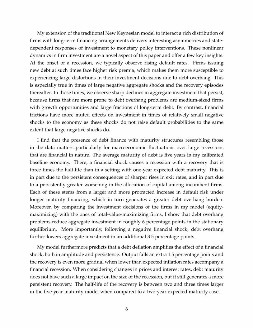
I start by delving into firm debt dynamics during the 2007 recession. I use time-seriesdata from the Financial Accounts of the United States (Flow of Funds). This datasetincludes flow of funds and balance sheet macro-level data at a quarterly frequency for1951Q4 - 2017Q3.1 All the nominal variables are deflated using the consumer price indexfor all urban consumers.

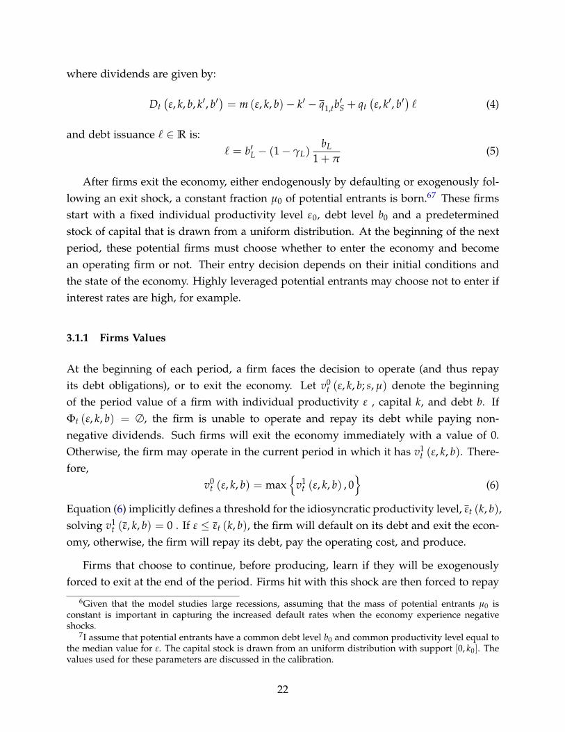
Figure 2(a) shows the build-up of debt in the corporate sector preceding the GreatRecession. The detrended total real debt increased sharply right from the onset of therecession. Figure 2(b) shows that this increased borrowing was accompanied by higherleverage, and was followed by a strong adjustment starting in 2009. Importantly, a largefraction of that adjustment came from long-term debt. Figure 2(c) shows that, afterthe recession ended, long-term borrowing fell and remained below trend for severalyears. Nevertheless, the sharp adjustment in total debt following the crisis increased therelevance of long-term debt, as seen in the increased long-term debt ratios in Figure 2(d).

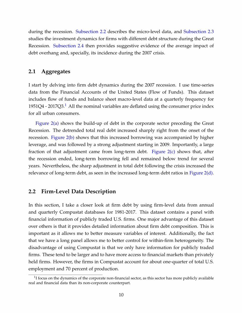
2.2 Firm-Level Data Description

In this section, I take a closer look at firm debt by using firm-level data from annualand quarterly Compustat databases for 1981-2017. This dataset contains a panel withfinancial information of publicly traded U.S. firms. One major advantage of this datasetover others is that it provides detailed information about firm debt composition. This isimportant as it allows me to better measure variables of interest. Additionally, the factthat we have a long panel allows me to better control for within-firm heterogeneity. Thedisadvantage of using Compustat is that we only have information for publicly tradedfirms. These tend to be larger and to have more access to financial markets than privatelyheld firms. However, the firms in Compustat account for about one-quarter of total U.S.employment and 70 percent of production.

1I focus on the dynamics of the corporate non-financial sector, as this sector has more publicly availablereal and financial data than its non-corporate counterpart.

10

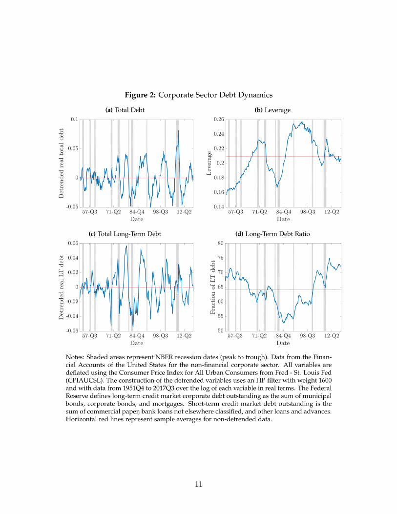
Figure 2: Corporate Sector Debt Dynamics

(a) Total Debt

57-Q3 71-Q2 84-Q4 98-Q3 12-Q2

Date

-0.05

0

0.05

0.1

Det

rended

realto

taldeb

t

(b) Leverage

57-Q3 71-Q2 84-Q4 98-Q3 12-Q2

Date

0.14

0.16

0.18

0.2

0.22

0.24

0.26

Lev

erage

(c) Total Long-Term Debt

57-Q3 71-Q2 84-Q4 98-Q3 12-Q2

Date

-0.06

-0.04

-0.02

0

0.02

0.04

0.06

Det

rended

realLT

deb

t

(d) Long-Term Debt Ratio

57-Q3 71-Q2 84-Q4 98-Q3 12-Q2

Date

50

55

60

65

70

75

80

Fra

ctio

nofLT

deb

t

Notes: Shaded areas represent NBER recession dates (peak to trough). Data from the Finan-cial Accounts of the United States for the non-financial corporate sector. All variables aredeflated using the Consumer Price Index for All Urban Consumers from Fred - St. Louis Fed(CPIAUCSL). The construction of the detrended variables uses an HP filter with weight 1600and with data from 1951Q4 to 2017Q3 over the log of each variable in real terms. The FederalReserve defines long-term credit market corporate debt outstanding as the sum of municipalbonds, corporate bonds, and mortgages. Short-term credit market debt outstanding is thesum of commercial paper, bank loans not elsewhere classified, and other loans and advances.Horizontal red lines represent sample averages for non-detrended data.

11

I delete observations of regulated, financial, and public service firms, as well as offoreign governments. I also eliminate observations with missing or negative values fortotal assets, capital expenditures, property, plant and equipment, cash holding or sales.Firms for which total assets are lower than cash holding, capital expenditures or prop-erty plant and equipment are not considered. I also drop firms for which the value oftotal assets is less than $0.5 million, as well as firms with asset growth or sales growth ex-ceeding 100%. Finally, I also delete firms for which the value of long-term debt exceedsthe value of total assets or the value of total debt. Finally, I only consider firms withat least 5 years (20 quarters) of investment spells. The resulting annual sample containsdata for 3,527 distinct firms across 34 years, for a total of 31,064 firm-year observations.Appendix A provides a more detailed description of the data construction.

My main measure for investment is the log change in net capital stock, ∆ log ki,t+1,where ki,t+1 is the capital stock of firm i at the end of period t. Alternatively, I also use(xi,t/ki,t), where xi,t is the gross change in the capital stock, to measure gross investmentrates. To characterize firm debt structure, I use measures related to both the fraction ofdebt that could generate rollover risk, as well as firm reliance on long-term financing,which, as is traditional in the literature, is defined as all debt issued with a maturityequal or longer than one year. For the latter, I use the ratio of total long-term debt tototal debt. For the former, this is, debt obligations that may not be rolled over, I breakthis down further into two variables: (1) the fraction of total debt that matures withina year and (2) the fraction of long-term debt maturing within the year. The advantageof using this second measure is the fact that it uses the fraction of long-term debt thatis due. This means that it can account for debt that has been issued prior to the currentperiod, and hence may be less susceptible to the choice of current investment.

Table 1 reports summary statistics for the sample used in the analysis below. Asseen there, the mean annual capital growth rate is about 7.1% with a standard deviationof 14.4%. The mean long-term debt ratio is 90%, but more than half of the firm-yearobservations in the sample have a unitary long-term debt ratio, thus highlighting theimportance of long-term financing. Within that long-term debt, on average, around12.3% matures within the next year, and 20.7% of all debt must also be paid within thenext year.

12

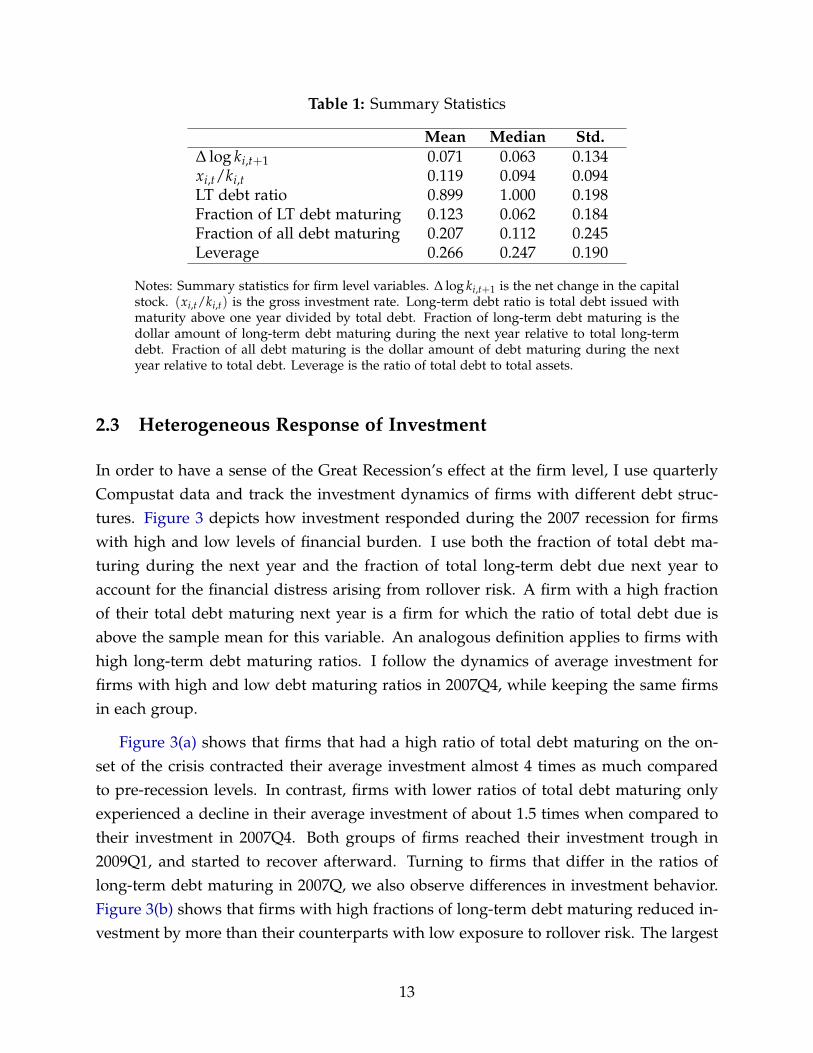
Table 1: Summary Statistics

Mean Median Std.∆ log ki,t+1 0.071 0.063 0.134xi,t/ki,t 0.119 0.094 0.094LT debt ratio 0.899 1.000 0.198Fraction of LT debt maturing 0.123 0.062 0.184Fraction of all debt maturing 0.207 0.112 0.245Leverage 0.266 0.247 0.190

Notes: Summary statistics for firm level variables. ∆ log ki,t+1 is the net change in the capitalstock. (xi,t/ki,t) is the gross investment rate. Long-term debt ratio is total debt issued withmaturity above one year divided by total debt. Fraction of long-term debt maturing is thedollar amount of long-term debt maturing during the next year relative to total long-termdebt. Fraction of all debt maturing is the dollar amount of debt maturing during the nextyear relative to total debt. Leverage is the ratio of total debt to total assets.

2.3 Heterogeneous Response of Investment

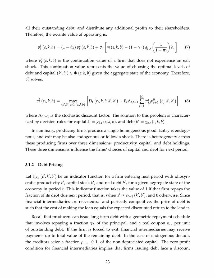
In order to have a sense of the Great Recession’s effect at the firm level, I use quarterlyCompustat data and track the investment dynamics of firms with different debt struc-tures. Figure 3 depicts how investment responded during the 2007 recession for firmswith high and low levels of financial burden. I use both the fraction of total debt ma-turing during the next year and the fraction of total long-term debt due next year toaccount for the financial distress arising from rollover risk. A firm with a high fractionof their total debt maturing next year is a firm for which the ratio of total debt due isabove the sample mean for this variable. An analogous definition applies to firms withhigh long-term debt maturing ratios. I follow the dynamics of average investment forfirms with high and low debt maturing ratios in 2007Q4, while keeping the same firmsin each group.

Figure 3(a) shows that firms that had a high ratio of total debt maturing on the on-set of the crisis contracted their average investment almost 4 times as much comparedto pre-recession levels. In contrast, firms with lower ratios of total debt maturing onlyexperienced a decline in their average investment of about 1.5 times when compared totheir investment in 2007Q4. Both groups of firms reached their investment trough in2009Q1, and started to recover afterward. Turning to firms that differ in the ratios oflong-term debt maturing in 2007Q, we also observe differences in investment behavior.Figure 3(b) shows that firms with high fractions of long-term debt maturing reduced in-vestment by more than their counterparts with low exposure to rollover risk. The largest

13

Figure 3: Firm Investment and Debt Structure During the Great Recession

(a) By Fraction of Total Debt Maturing

08Q3 09Q2 10Q1 10Q4 11Q3

Date

-4

-3

-2

-1

0

1

2

3

Deviationsof"logkt+

1from

2007Q4

Low total debt maturingHigh total debt maturing

(b) By Fraction of Long-Term Debt Maturing

08Q3 09Q2 10Q1 10Q4 11Q3

Date

-2.5

-2

-1.5

-1

-0.5

0

0.5

Deviationsof"logkt+

1from

2007Q4

Low LT debt maturingHigh LT debt maturing

Notes: Shaded areas represent NBER recession dates for the Great Recession (peak to trough).Fraction of all debt maturing is the dollar amount of debt maturing during the next yearrelative to total debt. Fraction of long-term debt maturing is the dollar amount of long-term debt maturing during the next year relative to total long-term debt. For both panels,the threshold between the two groups comes from the sample mean of each variable. Theaverage investment for each group is normalized with respect to their respective values in2007Q4.

contraction for high long-term debt maturing firms (2009Q3) was about 1.5 times thelargest contraction for the low long-term debt maturing firms (2009Q1). Although theseresults do not control by other firm characteristics, they provide suggestive evidenceabout the role of debt structure for investment dynamics.

2.4 Debt Overhang at the Firm Level

Leverage and the financial burden that arises from debt repayments are critical in under-standing the relevance of debt overhang on firm investment decisions. On the one hand,leverage provides an overall measure if firm indebtedness. On the other hand, firmswith a larger relative size of debt obligations are more likely to experience rollover risk.Together, these two variables are useful in gauging to what extent a firm is financiallyconstrained and how likely it is to default.

Leverage is a financial variable that has been found to be closely related to the cost ofexternal finance. Whited and Wu (2006), for example, document that highly leveragedfirms tend to be more financially constrained. Ottonello and Winberry (2018) find thatleverage is a major determinant of the response of firm investment to monetary policy

14

Table 2: Investment by Groups of Leverage and Debt Maturing

High leverage Low leverageMean Median Std Mean Median Std

High total debt maturing 0.050 0.049 0.155 0.073 0.067 0.131Low total debt maturing 0.070 0.060 0.140 0.078 0.068 0.122High LT debt maturing 0.041 0.042 0.157 0.070 0.064 0.133Low LT debt maturing 0.071 0.062 0.140 0.079 0.070 0.121

Notes: Investment is ∆ log ki,t+1. High leverage is leverage above the sample mean. Highfraction of total debt maturing is having this value above its sample mean. High fraction oflong-term debt maturing is having this value above its sample mean. Fraction of all debtmaturing is the dollar amount of debt maturing during the next year relative to total debt.Fraction of long-term debt maturing is the dollar amount of long-term debt maturing duringthe next year relative to total long-term debt. Leverage is the ratio of total debt to total assets.

shocks. Thus, can differences in investment rates, across groups of debt, be explained bydifferences in leverage? Table 2 presents the average, median and standard deviation ofannual investment rates for firms with high and low leverage, across groups organizedby fractions maturing debt. A firm-year is classified as high leverage if leverage for thatyear is above the sample mean for this variable. The groups across fractions of debtmaturing, for total debt and long-term debt, are computed as before.

As shown in the Table, highly leveraged firms exhibit significant differences in theiraverage and median investment rates when grouped by their fractions of debt maturing.These differences are irrespective of using total debt or long-term debt. For example,the average investment rate for firms with high leverage and high total debt maturingis 5 percent, while its counterpart for a highly leveraged firm with lower rollover riskis 7.3 percent. Further, although these same differences are smaller for firms with lowleverage levels, they are still sizable: for instance, the average investment rate is 0.5percent points larger for a firm with above-average ratios of total debt maturing thanfor firms with lower-than-average debt maturing. These results suggest that, while it isnecessary to account for differences in leverage across firms, we also need to look closelyat their debt structure when studying the determinants of firm investment.2

To control for other firm level variables while taking into account the effect of highlevels of leverage and, more importantly, of the financial burden associated to debt re-

2Figure C1 in Appendix C shows an scatter plot for investment, leverage and the ratio of long-termdebt maturing within the next year, using 2007 data as an example. The idea is similar: there is a greatdeal of dispersion in investment rates that cannot be captured by focusing on leverage only.

15

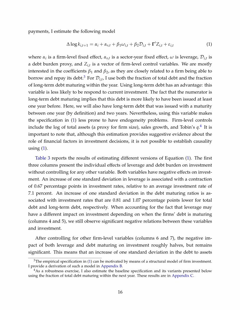
payments, I estimate the following model

∆ log ki,t+1 = αi + αs,t + β1ωi,t + β2Di,t + Γ′Zi,t + εi,t (1)

where αi is a firm-level fixed effect, αs,t is a sector-year fixed effect, ω is leverage, Di,t isa debt burden proxy, and Zi,t is a vector of firm-level control variables. We are mostlyinterested in the coefficients β1 and β2, as they are closely related to a firm being able toborrow and repay its debt.3 For Di,t, I use both the fraction of total debt and the fractionof long-term debt maturing within the year. Using long-term debt has an advantage: thisvariable is less likely to be respond to current investment. The fact that the numerator islong-term debt maturing implies that this debt is more likely to have been issued at leastone year before. Here, we will also have long-term debt that was issued with a maturitybetween one year (by definition) and two years. Nevertheless, using this variable makesthe specification in (1) less prone to have endogeneity problems. Firm-level controlsinclude the log of total assets (a proxy for firm size), sales growth, and Tobin’s q.4 It isimportant to note that, although this estimation provides suggestive evidence about therole of financial factors in investment decisions, it is not possible to establish causalityusing (1).

Table 3 reports the results of estimating different versions of Equation (1). The firstthree columns present the individual effects of leverage and debt burden on investmentwithout controlling for any other variable. Both variables have negative effects on invest-ment. An increase of one standard deviation in leverage is associated with a contractionof 0.67 percentage points in investment rates, relative to an average investment rate of7.1 percent. An increase of one standard deviation in the debt maturing ratios is as-sociated with investment rates that are 0.81 and 1.07 percentage points lower for totaldebt and long-term debt, respectively. When accounting for the fact that leverage mayhave a different impact on investment depending on when the firms’ debt is maturing(columns 4 and 5), we still observe significant negative relations between these variablesand investment.

After controlling for other firm-level variables (columns 6 and 7), the negative im-pact of both leverage and debt maturing on investment roughly halves, but remainssignificant. This means that an increase of one standard deviation in the debt to assets

3The empirical specification in (1) can be motivated by means of a structural model of firm investment.I provide a derivation of such a model in Appendix B.

4As a robustness exercise, I also estimate the baseline specification and its variants presented belowusing the fraction of total debt maturing within the next year. These results are in Appendix C.

16

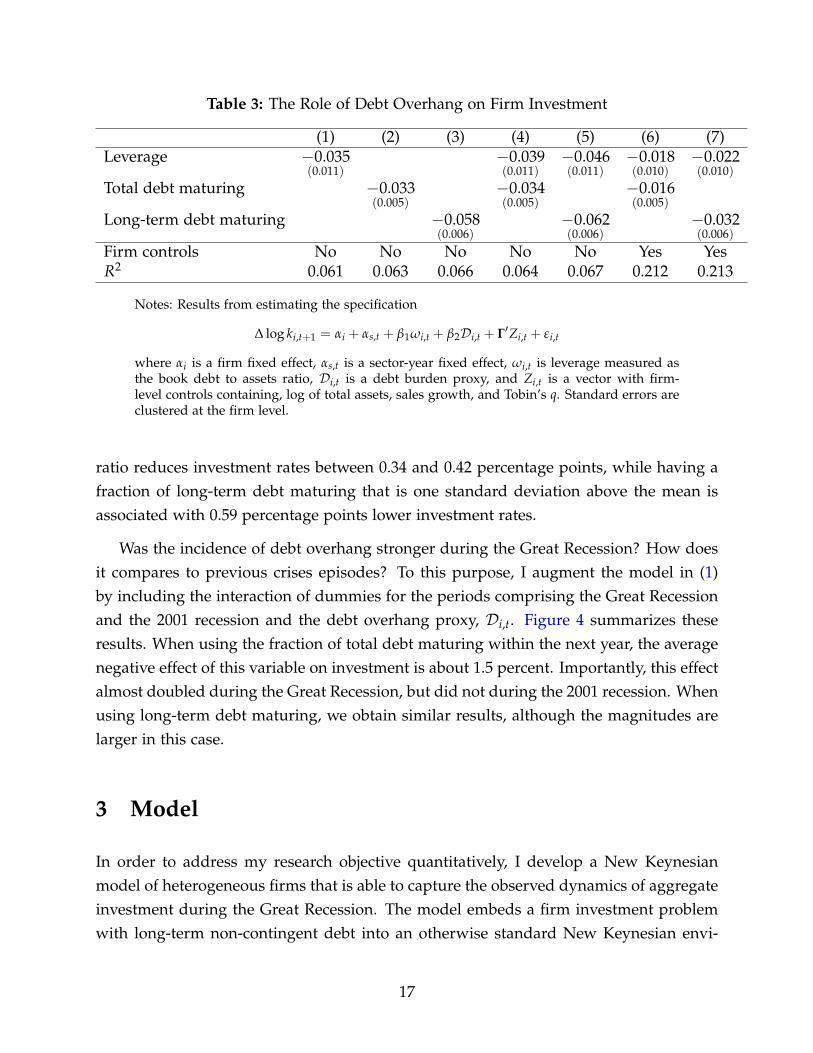
Table 3: The Role of Debt Overhang on Firm Investment

(1) (2) (3) (4) (5) (6) (7)Leverage −0.035

(0.011)−0.039(0.011)

−0.046(0.011)

−0.018(0.010)

−0.022(0.010)

Total debt maturing −0.033(0.005)

−0.034(0.005)

−0.016(0.005)

Long-term debt maturing −0.058(0.006)

−0.062(0.006)

−0.032(0.006)

Firm controls No No No No No Yes YesR2 0.061 0.063 0.066 0.064 0.067 0.212 0.213

Notes: Results from estimating the specification

∆ log ki,t+1 = αi + αs,t + β1ωi,t + β2Di,t + Γ′Zi,t + εi,t

where αi is a firm fixed effect, αs,t is a sector-year fixed effect, ωi,t is leverage measured asthe book debt to assets ratio, Di,t is a debt burden proxy, and Zi,t is a vector with firm-level controls containing, log of total assets, sales growth, and Tobin’s q. Standard errors areclustered at the firm level.

ratio reduces investment rates between 0.34 and 0.42 percentage points, while having afraction of long-term debt maturing that is one standard deviation above the mean isassociated with 0.59 percentage points lower investment rates.

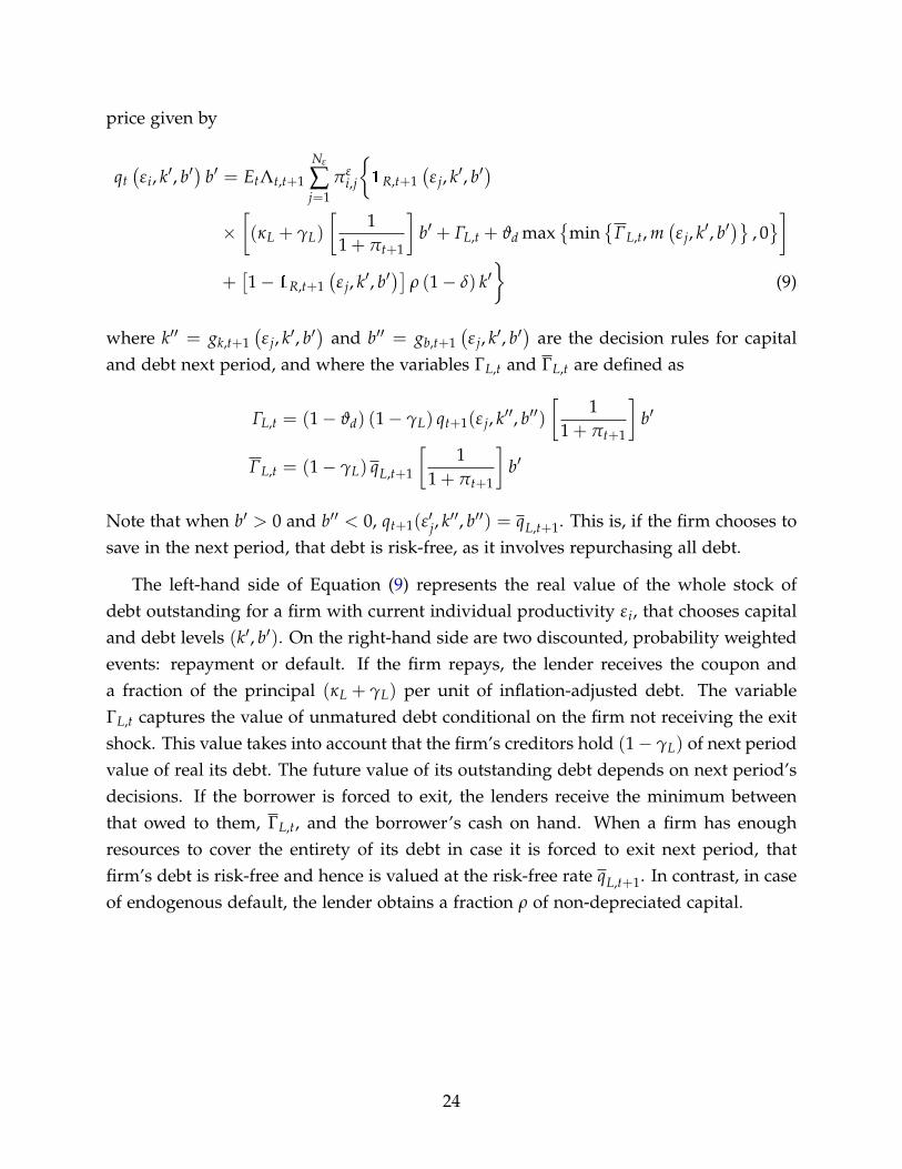
Was the incidence of debt overhang stronger during the Great Recession? How doesit compares to previous crises episodes? To this purpose, I augment the model in (1)by including the interaction of dummies for the periods comprising the Great Recessionand the 2001 recession and the debt overhang proxy, Di,t. Figure 4 summarizes theseresults. When using the fraction of total debt maturing within the next year, the averagenegative effect of this variable on investment is about 1.5 percent. Importantly, this effectalmost doubled during the Great Recession, but did not during the 2001 recession. Whenusing long-term debt maturing, we obtain similar results, although the magnitudes arelarger in this case.

3 Model

In order to address my research objective quantitatively, I develop a New Keynesianmodel of heterogeneous firms that is able to capture the observed dynamics of aggregateinvestment during the Great Recession. The model embeds a firm investment problemwith long-term non-contingent debt into an otherwise standard New Keynesian envi-

17

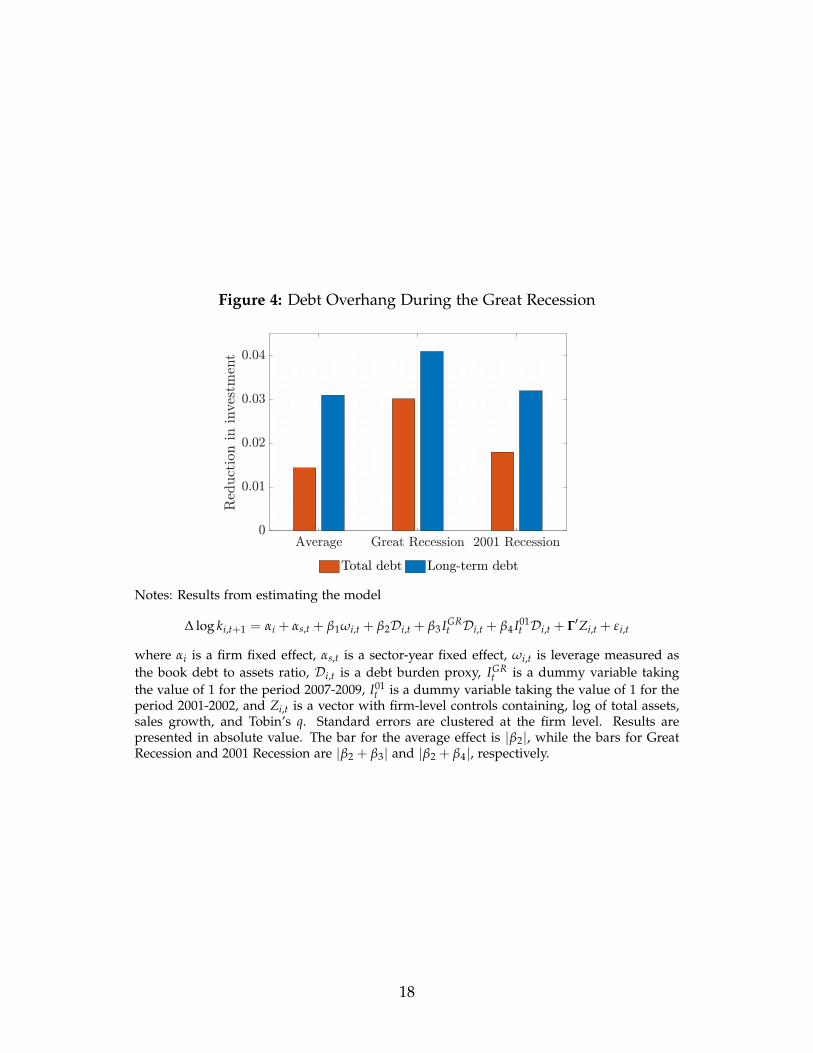
Figure 4: Debt Overhang During the Great Recession

Average Great Recession 2001 Recession0

0.01

0.02

0.03

0.04

Red

uct

ion

inin

ves

tmen

t

Total debt Long-term debt

Notes: Results from estimating the model

∆ log ki,t+1 = αi + αs,t + β1ωi,t + β2Di,t + β3 IGRt Di,t + β4 I01

t Di,t + Γ′Zi,t + εi,t

where αi is a firm fixed effect, αs,t is a sector-year fixed effect, ωi,t is leverage measured asthe book debt to assets ratio, Di,t is a debt burden proxy, IGR

t is a dummy variable takingthe value of 1 for the period 2007-2009, I01

t is a dummy variable taking the value of 1 for theperiod 2001-2002, and Zi,t is a vector with firm-level controls containing, log of total assets,sales growth, and Tobin’s q. Standard errors are clustered at the firm level. Results arepresented in absolute value. The bar for the average effect is |β2|, while the bars for GreatRecession and 2001 Recession are |β2 + β3| and |β2 + β4|, respectively.

18

ronment. I build on the work of Khan, Senga and Thomas (2016) and Ottonello andWinberry (2018), extended in three important dimensions. First, compared to Khan,Senga and Thomas (2016), I introduce nominal rigidities. Second, in contrast to bothKhan, Senga and Thomas (2016) and Ottonello and Winberry (2018), I incorporate long-term financing in order to study the effect of debt overhang on investment decisions,and allow for the possibility of having a binding zero-lower-bound constraint. Theseare important dimensions for understanding the role of financial frictions in the GreatRecession. Third, the model accounts for the possibility of having a binding zero-lower-bound constraint for the conduct of monetary policy, which was an important dimensionof the Great Recession.

Time is discrete and infinite. The economy is inhabited by six types of agents: (1)a continuum of identical households, (2) a representative final goods producer, (3) acontinuum of monopolistically competitive retailers, (4) infinitely-many perfectly com-petitive producers that are heterogeneous in their individual productivity, capital anddebt positions, (5) a continuum of risk-neutral financial intermediaries operating in per-fect competition, and (6) a central bank. The model considers three sources of aggregatefluctuations in a perfect foresight environment: TFP shocks, monetary shocks, and fi-nancial shocks.

Households own the firms and optimally choose their labor supply, consumption,and savings. To choose their level of savings, they buy a risk-free asset offered by thefinancial sector. Producers decide their optimal scale of production by choosing theirdemand for labor and capital to produce a single homogeneous good. These firms arealso able to issue defaultable nominal long-term debt that is purchased by financialintermediaries.

Retailers buy the homogeneous good from producers and differentiate it. Since theyare monopolistically-competitive, they choose the nominal price for the retail good theyproduce. However, in doing so, retailers are subject to price adjustment costs. Finalgoods producers combine all these differentiated retail goods by using a constant returnto scale production function. These firms sell their homogeneous good to householdsand firms, as consumption and investment goods, respectively. Finally, the central bankfollows a Taylor rule to determine the policy interest rate while, at the same time, beingsubject to a zero-lower-bound constraint. I present a detailed description of the modelbelow.

19

3.1 Producers

Producers differ in their capital, k, real debt outstanding, b, and individual productivity,ε, and produce a homogeneous good by combining capital and labor, n, according to adecreasing returns-to-scale technology; y = zεkαnν, where α, ν ∈ (0, 1) and α + ν < 1.Here, z represents aggregate total factor productivity, while ε denotes an idiosyncraticproductivity shock. I assume that the firm-specific shock ε ∈ E = {ε1, ε2, . . . , εNε} followsa Markov chain with transition probability Pr(ε′ = ε j| ε = εi) = πε

i,j ≥ 0 and ∑Nεj=1 πε

i,j = 1for every i = 1, 2, . . . , Nε. These firms sell their output to retail firms at price pw

t .

At the beginning of every period, a firm is identified by its capital stock, k ∈ K ∈R+, outstanding debt, b ∈ B ∈ R, and individual productivity, ε ∈ E. Therefore, wehave a distribution of firms µt (k, b, ε) over the support determined by the product spaceK×B×E. This implies that the aggregate state will be a combination of this distributionas well as the aggregate shocks to the economy. For notational simplicity, I subsume theaggregate state composed by the distribution of production firms, the aggregate nominalprice level, and the three aggregate disturbances in the time subscript.

Firms must choose their demand for labor and next’s period capital (investment). Iassume no capital adjustment frictions. To finance their investment expenditure, firmscan issue nominal long-term, non-contingent defaultable bonds at the price qt (ε, k′, b′).I assume that these bonds last forever (this means they are consols) and follow a repay-ment schedule that declines geometrically, so that, in each period any particular firmrepays a fraction γL of its principal. Hence, for a given γL, the average debt maturityis 1/γL. Note that, despite γL being common across firms, they will generally differ inthe amount of debt that is maturing at any given period. In addition to the amortizationof the principal, the firm also pays a fixed coupon κL per unit of outstanding debt. If,given the characteristics of the issuing firm, its debt is risk-free, its price is the risk-freediscount factor qL,t. Importantly, while firms are operated by their shareholders, credi-tors are first in the pecking order when a firm defaults. This arrangement is at the heartof the debt overhang problem. In addition to issuing debt, firms can also accumulatesavings. They do so using a one-period risk-free bond with price q1,t.

5 However, due tothe cost associated with long-term bonds, firms never choose to hold both savings anddebt at the same time. Therefore, we can denote negative values of debt as financialsavings, bS = −min {b, 0} ∈ R+, and similarly, outstanding debt can be denoted by

5The prices of the one-period bond used to save, q1,t, and the long-maturity debt, qL,t, are in generaldifferent, as the latter include the expected discounted sum of future payoffs associated to the coupon andprincipal.

20

bL = max {b, 0} ∈ R+.

At the beginning of each period, firms decide whether to operate or exit the economy.If they choose to operate, they must pay a fixed cost ξ0 and fulfill their debt obligations.Firms may avoid paying the fixed operating cost by exiting and defaulting on their debt.In this case, a defaulting firm (i.e., its shareholders) walks away with a value of 0, whilecreditors seize the firm’s assets. Define cash-on-hand for an operating firm of type(ε, k, b) as

mt (ε, k, b) = Πt (ε, k) +1

1 + π t[bS − (κL + γL) bL] + (1− δ) k− ξ0 − ξm,t (ε) (2)

where Πt (ε, k) = maxn (1− ν) pwt yt (ε, k, n) − wtn are flow profits, 1 + πt = Pt/Pt−1

is the inflation rate, Pt is the nominal price level, wt is the equilibrium wage rate andδ ∈ (0, 1) the depreciation rate of capital. Recall that either bS > 0 or bL > 0, butnot both. The second term in brackets in Equation (2) represents debt obligations: afirm entering the period with inflation-adjusted debt bL/ (1 + πt) must repay a fractionγL of it. In addition, it must also pay a coupon κL per unit of debt. The last term,ξm,t (ε), is an aggregate financial shock that affects firms’ balance sheets and makes themmore sensitive to financial frictions. It is modeled as proportional to the realization ofthe idiosyncratic productivity level, so that more productive firms experience a largerdisturbance than low productivity firms. This dependence on ε implies that, as firmsface uncertainty about their individual productivity, financial shocks increase risk andvolatility among producers.

Each firm also faces an exogenous exit shock. The probability of being exogenouslyforced to exit is ϑd. Operating firms receiving this shock sell all their capital, take nonew debt, and repay their creditors. If funds are sufficient, the firm walks away withwhatever is left and distributes it among its shareholders, otherwise the firm exits witha value to shareholders of 0.

A firm that knows it will continue into the next period then faces the decision ofchoosing the capital level to operate in the next period, k′, and the debt level (or savings),b′, to take. When doing so, firms face a non-negativity restriction on their dividends thatprevent them from raising funds by issuing equity. Define the set of feasible choices of(k′, b′) as:

Φt (ε, k, b) ={(

k′, b′)∈ R+ ×R|Dt

(ε, k, b, k′, b′

)≥ 0

}(3)

21

where dividends are given by:

Dt(ε, k, b, k′, b′

)= m (ε, k, b)− k′ − q1,tb

′S + qt

(ε, k′, b′

)` (4)

and debt issuance ` ∈ R is:` = b′L − (1− γL)

bL

1 + π(5)

After firms exit the economy, either endogenously by defaulting or exogenously fol-lowing an exit shock, a constant fraction µ0 of potential entrants is born.67 These firmsstart with a fixed individual productivity level ε0, debt level b0 and a predeterminedstock of capital that is drawn from a uniform distribution. At the beginning of the nextperiod, these potential firms must choose whether to enter the economy and becomean operating firm or not. Their entry decision depends on their initial conditions andthe state of the economy. Highly leveraged potential entrants may choose not to enter ifinterest rates are high, for example.

3.1.1 Firms Values

At the beginning of each period, a firm faces the decision to operate (and thus repayits debt obligations), or to exit the economy. Let v0

t (ε, k, b; s, µ) denote the beginningof the period value of a firm with individual productivity ε , capital k, and debt b. IfΦt (ε, k, b) = ∅, the firm is unable to operate and repay its debt while paying non-negative dividends. Such firms will exit the economy immediately with a value of 0.Otherwise, the firm may operate in the current period in which it has v1

t (ε, k, b). There-fore,

v0t (ε, k, b) = max

{v1

t (ε, k, b) , 0}

(6)

Equation (6) implicitly defines a threshold for the idiosyncratic productivity level, εt (k, b),solving v1

t (ε, k, b) = 0 . If ε ≤ εt (k, b), the firm will default on its debt and exit the econ-omy, otherwise, the firm will repay its debt, pay the operating cost, and produce.

Firms that choose to continue, before producing, learn if they will be exogenouslyforced to exit at the end of the period. Firms hit with this shock are then forced to repay

6Given that the model studies large recessions, assuming that the mass of potential entrants µ0 isconstant is important in capturing the increased default rates when the economy experience negativeshocks.

7I assume that potential entrants have a common debt level b0 and common productivity level equal tothe median value for ε. The capital stock is drawn from an uniform distribution with support [0, k0]. Thevalues used for these parameters are discussed in the calibration.

22

all their outstanding debt, and distribute any additional profits to their shareholders.Therefore, the ex-ante value of operating is:

v1t (ε, k, b) = (1− ϑd) v2

t (ε, k, b) + ϑd

[m (ε, k, b)− (1− γL) qL,t

(1

1 + πt

)bL

](7)

where v2t (ε, k, b) is the continuation value of a firm that does not experience an exit

shock. This continuation value represents the value of choosing the optimal levels ofdebt and capital (k′, b′) ∈ Φ (ε, k, b) given the aggregate state of the economy. Therefore,v2

t solves:

v2t (εi, k, b) = max

(k′,b′)∈Φt(εi,k,b)

[Dt(εi, k, b, k′, b′

)+ EtΛt,t+1

Nε

∑j=1

πεi,jv

0t+1(ε j, k′, b′

)](8)

where Λt,t+1 is the stochastic discount factor. The solution to this problem is character-ized by decision rules for capital k′ = gk,t (ε, k, b), and debt b′ = gb,t (ε, k, b).

In summary, producing firms produce a single homogeneous good. Entry is endoge-nous, and exit may be also endogenous or follow a shock. There is heterogeneity acrossthese producing firms over three dimensions: productivity, capital, and debt holdings.These three dimensions influence the firms’ choices of capital and debt for next period.

3.1.2 Debt Pricing

Let 1R,t (ε′, k′, b′) be an indicator function for a firm entering next period with idiosyn-

cratic productivity ε′, capital stock k′, and real debt b′, for a given aggregate state of theeconomy in period t. This indicator function takes the value of 1 if that firm repays thefraction of its debt due next period, that is, when ε′ ≥ εt+1 (k′, b′), and 0 otherwise. Sincefinancial intermediaries are risk-neutral and perfectly competitive, the price of debt issuch that the cost of making the loan equals the expected discounted return to the lender.

Recall that producers can issue long-term debt with a geometric repayment schedulethat involves repaying a fraction γL of the principal, and a real coupon κL, per unitof outstanding debt. If the firm is forced to exit, financial intermediaries may receivepayments up to total value of the remaining debt. In the case of endogenous default,the creditors seize a fraction ρ ∈ [0, 1] of the non-depreciated capital. The zero-profitcondition for financial intermediaries implies that firms issuing debt face a discount

23

price given by

qt(εi, k′, b′

)b′ = EtΛt,t+1

Nε

∑j=1

πεi,j

{1R,t+1

(ε j, k′, b′

)×[(κL + γL)

[1

1 + πt+1

]b′ + ΓL,t + ϑd max

{min

{ΓL,t, m

(ε j, k′, b′

)}, 0}]

+[1− 1R,t+1

(ε j, k′, b′

)]ρ (1− δ) k′

}(9)

where k′′ = gk,t+1(ε j, k′, b′

)and b′′ = gb,t+1

(ε j, k′, b′

)are the decision rules for capital

and debt next period, and where the variables ΓL,t and ΓL,t are defined as

ΓL,t = (1− ϑd) (1− γL) qt+1(ε j, k′′, b′′)[

11 + πt+1

]b′

ΓL,t = (1− γL) qL,t+1

[1

1 + πt+1

]b′

Note that when b′ > 0 and b′′ < 0, qt+1(ε′j, k′′, b′′) = qL,t+1. This is, if the firm chooses to

save in the next period, that debt is risk-free, as it involves repurchasing all debt.

The left-hand side of Equation (9) represents the real value of the whole stock ofdebt outstanding for a firm with current individual productivity εi, that chooses capitaland debt levels (k′, b′). On the right-hand side are two discounted, probability weightedevents: repayment or default. If the firm repays, the lender receives the coupon anda fraction of the principal (κL + γL) per unit of inflation-adjusted debt. The variableΓL,t captures the value of unmatured debt conditional on the firm not receiving the exitshock. This value takes into account that the firm’s creditors hold (1− γL) of next periodvalue of real its debt. The future value of its outstanding debt depends on next period’sdecisions. If the borrower is forced to exit, the lenders receive the minimum betweenthat owed to them, ΓL,t, and the borrower’s cash on hand. When a firm has enoughresources to cover the entirety of its debt in case it is forced to exit next period, thatfirm’s debt is risk-free and hence is valued at the risk-free rate qL,t+1. In contrast, in caseof endogenous default, the lender obtains a fraction ρ of non-depreciated capital.

24

3.2 Retailers

There is a continuum of mass 1 of ex-ante identical retailers indexed by i.8 Each retailerproduces the differentiated variety yi,t using the linear production function yi,t = yi,t,where yi,t is a wholesale good purchased from the production firms by retailer i at pricepw

t . These firms operate in a monopolistically competitive market, so they set the priceof their variety, Pi,t, subject to its demand curve (from final goods producers). Whenchoosing their optimal price, these firms are subject to quadratic adjustment costs:

ψp

2

(Pi,t

Pi,t−1− 1)2

Yt (10)

3.3 Final Goods Producers

The representative firm producing final goods combines the continuum of differenti-ated goods produced by retailers and then sells a homogeneous good in a perfectlycompetitive market at price Pt to households (as consumption) and producing firms (asinvestment). Its production technology is:

Yt =

[∫ 1

0y

θ−1θ

i,t di] θ

θ−1

(11)

where θ is the elasticity of substitution over varieties of the retail good. These firmsmaximize profits subject to (11).

3.4 Households

There is a continuum of identical households that consume, c, and supply labor to pro-ducers, n. They discount the future at the rate β ∈ (0, 1) and save by means of a nominalrisk-free bond that pays the interest rate it−1. Let a denote real holdings of the risk-freeasset. Households also own all firms in the economy. More specifically, they hold shares,s, of each production firm. These shares have a real price m0,t, which includes the value

8Including these retail firms implies that there is an extra layer in how we model production in thiseconomy when compared to New Keynesian models without production heterogeneity. As discussed in?, including retail firms allows us to incorporate price rigidities in a tractable manner. In presence ofheterogeneity and financial frictions, this set up lets us separate the production-investment problem andthe price-setting problem in a simple way.

25

of dividends, and an ex-dividend real price m1,t. As households also own the retailers,they also receive their profits, denoted by Πr

t , which are paid in a lump-sum fashion.

Their preferences are summarized by the period utility function U (c, 1− n) and solvethe following problem

Wt (s, a) = maxc,n,s′,a′

{U (c, 1− n) + βEtWt+1

(s′, a′

)}(12)

subject to their budget constraint, which in real terms is given by:

c + a′ +∫

m1,t(ε′, k′, b′

)s′(d[ε′, k′, b′

])≤ wtn +

(1 + it−1

1 + πt

)a +

∫m0,t (ε, k, b) s (d [ε, k, b]) + Πr

t (13)

3.5 Central Bank

The central bank of this economy sets the short-term nominal interest rate following aTaylor rule and is subject to a zero-lower-bound constraint:

1 + it = max

{1,(1 + i

) (1 + πt

1 + π

)φπ(

yt

y

)φy

exp(

εit

)}(14)

Here, it is the nominal policy rate, i is its stationary value, π is the inflation target, y isthe steady state level of output, and εi

t is an i.i.d. shock to the nominal interest rate thatsatisfies εi

t ∼ N(0, σ2

i). The parameters φπ and φy measure the response of monetary

policy to deviations in inflation with respect to its targeted value, and deviations inoutput with respect to its stationary value, respectively.

3.6 Equilibrium

Definition 1. The competitive equilibrium of this model is a set of functions for valuesv0

t (ε, k, b), v1t (ε, k, b), v2

t (ε, k, b), decision rules k′ = gk,t (ε, k, b), b′ = gb,t (ε, k, b), εt (k, b),n (ε, k, b), allocations Yt, Xt, Ξt, Πr

t , prices pwt , wt, q1,t, qL,t, πt, qt (ε, k′, b′), and a distribu-

tion µt (ε, k, b), such that, given the aggregate shocks(zt, ξm,t, εi

t):

1. The values v0t (ε, k, b), v1

t (ε, k, b), and v2t (ε, k, b), and the decision rules k′ = gk,t (ε, k, b),

b′ = gb,t (ε, k, b), εt (k, b), and n (ε, k, b) solve the production firm problem described

26

by (2) - (8), given prices pwt , wt, q1,t, qL,t, πt, and qt (ε, k′, b′).

2. Financial intermediaries price debt priced according to Equation (9).

3. Retailers solve their price optimization problem and final goods producers deter-mine the optimal demand for varieties of the retail good, taking prices as given.

4. Households solve their problem in (12) and (13).

5. The central bank sets nominal short-term interest rates according to (14).

6. The distribution of firms is consistent with the production firms’ and potentialentrants’ decision rules:

µt+1(ε′, k′, b′

)= (1− ϑd)

Nε

∑i=1

∫{(gk,t(εi,k,b),gb,t(εi,k,b))=(k′,b′)}

1 {εi ≥ εt (k, b)} µ ([dk× db])

+∫{(k0,b0)=(k′,b′)}

1 {ε0 ≥ εt (k, b)} µ0 ([dk0 × db0]) (15)

where gb,t (ε, k, b) = gb,t (ε, k, b) / (1 + πt+1).

7. Markets clear: markets for goods, labor and assets clear. Denoting aggregate in-vestment by Xt, and total operating costs for production firms by Ξt, the aggregateresource constraint holds:

Yt = Ct + Xt + Ξt +ψp

2π2

t Yt (16)

Households and Risk-Free Rates

Imposing market clearing, households’ labor-leisure condition and the Euler equationfor bonds pin down the equilibrium wage and the stochastic discount factor:

λt = D1U (C, 1− N) (17)

wt = D2U (C, 1− N) /λt (18)

Λt,t+1 = βλt+1/λt (19)

The Euler equation for bonds also implies that the risk-less discount factor for the one-period bond is q1,t = EtΛt,t+1/ (1 + πt+1). Finally, considering a risk-less bond on the

27

debt pricing equation (9) yields the following risk-free discount factor for long-term debt:

qL,t = EtΛt,t+1

(1

1 + πt+1

) [(κL + γL) + (1− γL) qL,t+1

](20)

This means that the current price of risk-less long-term debt is equal to the the expecteddiscounted sum of payments next period (coupon and a fraction of principal) and thenext period price of the remaining outstanding fraction of the bond.

Retailers and Final Goods Producers

The solution to the final good producers’ problem is a demand function for each varietyi ∈ [0, 1]:

yi,t =

(Pi,t

Pt

)−θ

Yt (21)

where Pi,t is the price of variety i, and

Pt =

(∫ 1

0P1−θ

i,t di) 1

1−θ

(22)

is the price index. Note that the price index of the retail goods is equal to the price ofthe final good, as final goods producers set their price equal to their marginal cost.

Taking the demand function in (21) as given, and noting that retailers are symmetric,the solution to their problem yields the following New Keynesian Phillips curve:

πt (1 + πt) =1

ψp[θpw

t − (θ − 1)] + EtΛt,t+1πt+1 (1 + πt+1)Yt+1

Yt(23)

Producers

We can divide the population of firms in the economy in three groups: unconstrained,partially constrained and risky. An unconstrained firm has accumulated enough as-sets so that is able to finance its efficient level of capital9 while remaining permanentlyunconstrained. These firms, not being sensitive to financial conditions, and having out-grown financial frictions, have a marginal valuation of internal funds that is equal to λ,

9The efficient or frictionless level of capital, k∗t (ε), solves

28

and hence are indifferent between financial savings and dividends. To resolve this inde-terminacy, I assume that these firms implement a minimum savings policy that insuresthat they will remain financially unconstrained under any possible sequence of futureshocks. This debt policy (minimum savings policy) solves:

b∗t (εi) = min

{min

(ε j,zt)|πεi,jπ

zt >0

bt+1(k∗t (εi) , ε j

), 0

}(24)

where

bt (k, ε) = (1 + πt) [Πt (ε, k) + (1− δ) k− ξ0 − ξm,t (ε)]

+ (1 + πt)min{[−k∗ (ε) + q1,tb

∗t (ε)

], 0}

(25)

Since firms issue long-term debt, the presence of exogenous default risk implies thatall firms with positive outstanding debt are risky and, hence, not permanently uncon-strained. Hence, it is important to constraint b∗t (ε) ≤ 0. By construction, unconstrainedfirms are therefore able to pay positive dividends while implementing their frictionlesslevel of capital and the minimum savings policy.

Partially constrained firms do not face an immediate default risk, but have not yetaccumulated enough assets to guarantee that that will be the case in any possible future.As they have not outgrown financial constraints permanently, their valuation of retainedearnings exceeds the marginal utility of consumption, λ. Therefore, for these firms itis optimal to implement a zero-dividend policy while setting k′ = k∗ (ε) and b′ = b′ asimplied by their budget constraint and that can be either positive or negative. Naturally,that choice of (k′, b′) must be such that the probability of default next period is 0. Thismeans that if b′ > 0, it must be the case that

m′t+1(ε j, k∗, b′ (k∗; εi, k, b)

)≥ (1− γL) qL,t+1b′ (k∗; εi, k, b) (26)

for all j such that πεi,j > 0.

Finally, risky firms face positive risk premium as their immediate default risk is alsopositive. This implies that they borrow at qt (ε, k′, b′) < qL,t. Such firms, having a highershadow value of internal funds, do not pay dividends. Risky firms must solve (6) - (8)

k∗t (ε i) = argmaxk′

{−k′ + Λt,t+1

Nε

∑j=1

πεi,j[Πt+1

(ε j, k′

)+ (1− δ) k′

]}

29

subject to (9) and, in general, will not adopt the frictionless capital stock.

4 Calibration

In the model economy, one period represents a year. The calibration is such that thestationary equilibrium of the model replicates some aggregate and firm-level momentswhen the the economy is absent of aggregate uncertainty. The real interest rate is setto 4 percent and the annual inflation rate is fixed to 2 percent. The depreciation rate isset to 7.68 percent, consistent with the average between 1947 and 2016 for current-costdepreciation in the Fixed Asset Tables from NIPA. The parametersprs of the productionfunction, α and ν are set to obtain a capital to output ratio of 2.3 and a labor share ofoutput of 0.6. The scale parameter that measure the preference for leisure, ϕ is used toreplicate that households work one-third of their unit of available time.

The stochastic process for idiosyncratic productivity is obtained after approximatingthe following autoregressive process for ε: log ε′ = ρε log ε + η′ε, where ηε is i.i.d. dis-tributed N

(0, σ2

ε

). The approximation uses the Tauchen method for Nε = 9 grid points.

The characteristics of potential entrants are fixed so that they have individual produc-tivity ε = ε7 and initial debt b = 0.08, while their capital is drawn from a uniformdistribution with support on

[0, k]. The calibration also targets the average debt to book

asset ratio. Using a panel constructed with the micro data from the Quarterly FinancialReports, Crouzet and Mehrotra (2018) document that the average gross leverage at thefirm-level is 0.35. Dinlersoz et al. (2018), using a dataset that matches firm-level datafrom the LBD database with balance sheet data for privately held and publicly listedfirms, find that the average firm-level gross leverage is 0.46 and 0.56 for private andpublic firms, respectively. These estimates of leverage for U.S. firms are higher than thevalue of 0.27 reported in Table 1. I chose to target this latter value despite it may under-estimate the effect of financial frictions and long-term debt, so that the other momentsof the model can be directly comparable to the sample used in Section 2.

Annual Compustat data, despite having information about debt maturity structure,lumps all debt with maturity longer than, or equal to, five years together. Guedes andOpler (1996), using a database with corporate debt issues between 1982 and 1993, docu-ment that the average and median maturity are 12 and 10 years, respectively. They alsofind that the average Macaulay duration (computed by weighting the average maturityof cashflows) of corporate debt issues is 6 years. Using data from the Mergent Fixed In-

30

come Securities Database (FISD), a database that reports issue details on corporate debtissues (among others), I find that the mean and median maturity of corporate debt at theoffering date for the period 1984-2018 is 10.1 and 8.2 years, respectively.10 I therefore setthe value for the parameter γL to 0.2, which implies an average maturity of 5 years. Thisvalue is conservative in measuring the incidence of long-term financing, but it is con-sistent with the fact that, on average, firms have 20 percent of their debt maturing eachyear, as reported in Section 2. It also accounts for the fact that the durations obtainedfrom Guedes and Opler (1996) and the FISD database are computed for public corporatedebt issues, which tend to have longer maturity. The coupon rate, κL, is chosen to implya price of risk-free debt equal to 1 in steady state, as in Gomes et al. (2016). The capitalrecovery rate is set to 45.7 percent, according to what the Moody’s Default Risk Servicereports to be the average of recovery rate for the period 1978-2010.

The parameters(

ξ0, ρε, σε, ϑd, k)

are jointly set to replicate (i) a default rate of 2%, (ii)an exit rate of 10%, (iii) a debt to capital ratio of 0.266, (iv) an average employment ofentrants relative to incumbents of 10%, (v) an average investment rate across continuingfirms of 0.122, (vi) a standard deviation is those investment rate of 0.337, (vii) an averagespread of 2.35 as documented by Gilchrist and Zakrajšek (2012). The elasticity of substi-tution between varieties of the retail good is set to 11, so that the steady state markup is10 percent. As in Kaplan et al. (2018), the adjustment cost parameter, ψp, is fixed to 100to imply a slope of 0.1 in the Phillips curve. Finally, the response of monetary policy todeviations in the inflation rate, φπ, is set to 1.5.

5 Stationary Equilibrium

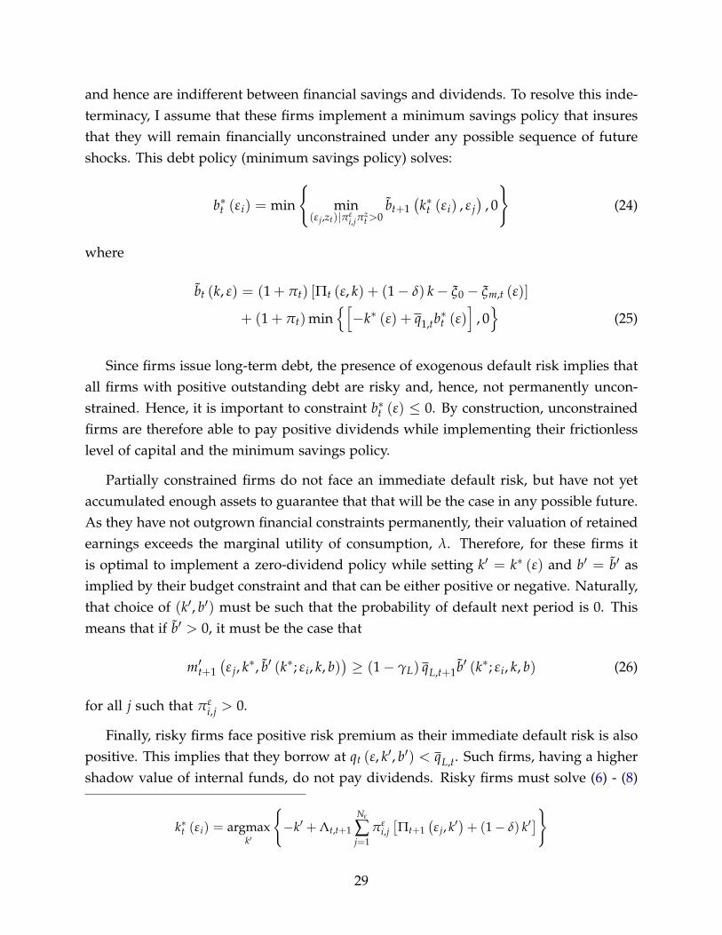
Figure 5 presents the distribution of production firms over capital and leverage as firmsenter any given period in the stationary equilibrium. Capital increases from left to right,and leverage raises front to back along the left axis. Negative levels of leverage representsavings relative to capital. Safe firms are directly identifiable. They are along each oneof the 9 (one per realization of ε) lines in which capital remains constant. Each one ofthese lines contains firms that are implementing the efficient level of capital associatedto their idiosyncratic productivity. Among those safe firms there is sizable heterogeneity,

10I use the Mergent FISD data from 1984 to 2018 and apply the same filters used with Compustat datain Section 2. This means that utilities, financial institutions, public administration entities and foreign gov-ernments are excluded from the sample. I also exclude issues not denominated in U.S. dollars, convertiblebonds, asset-backed bonds and preferred bonds, as well as issues of firms that are not incorporated in theU.S.

31

Table 4: Targeted Moments

Target Model DataDefault rate 1.51 2.0Exit rate 9.51 10.0Entry rate 9.39 10.0Average leverage 0.37 0.266Standard deviation leverage 0.31 0.364Mean n of entrants (r/ incumbents) 0.07 0.10Mean investment rate 0.15 0.122Standard deviation of investment rates 0.39 0.337Capital to output ratio 2.06 2.3Mean credit spread 1.14 2.35Recovery rate - 0.457Average maturity - {5, 9.8}

as we have move from safe borrowers in the regions with higher concentration, to firmswith large amounts of savings. Right behind each one of these lines there are firms thatare transitioning from facing a positive default premia to safe borrowing. Those firms,however, cannot yet implement their frictionless level of capital.

Near the right side of the figure, we have a concentration of firms that can be dividedinto two groups. The first group is comprised by entrants and by asset poor firmsholding low levels of capital and high levels of debt, with leverage levels between 1 and3. These firms, despite being in a very vulnerable position and facing high credit spreads(see Figure 6), are not guaranteed to exit this period or the next as the long maturity offinancing eases their financial burden compared to a one-period debt model in whichall debt is due. The second group of firms are also capital poor, but their leveragelevels are so high that they will exit without producing. They arrived in to this regionafter implementing a risky strategy in which they were betting on a small probability ofdrawing a high level of productivity, while holding previously issued debt.

The endogenous determination of an schedule for the price of debt is at the core ofthe model. In Equation (9), the price of debt increases in capital and idiosyncratic pro-ductivity, and decreases in debt. Equivalently, the more leverage (because of increaseddebt or reduced capital) the lower the price of debt. Figure 6 depicts this result. Fig-ure 6(a) considers the case of high productivity and a low productivity firms for whichthe choice of capital, k′, is fixed. The price of debt for these firms (at which all theirdebt is valued, including new issues) falls as b′ increases to account for the increaseddefault risk. However, having higher productivity counteracts, at least partially, part

32

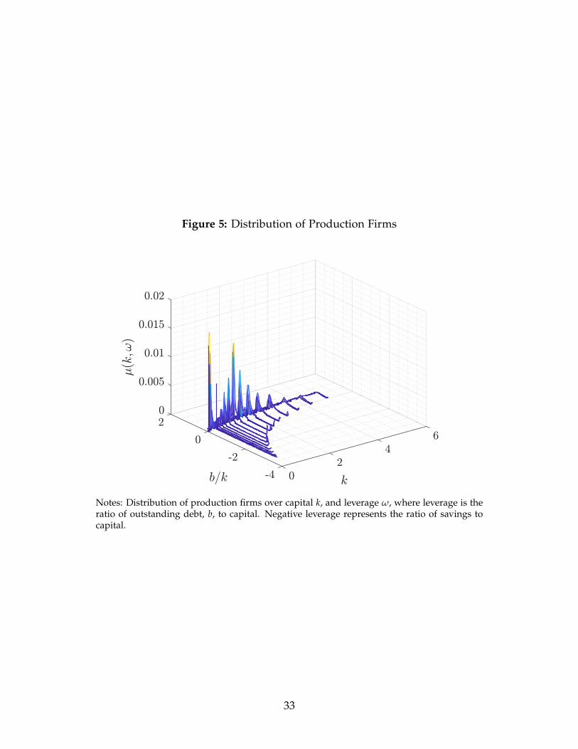
Figure 5: Distribution of Production Firms

Notes: Distribution of production firms over capital k, and leverage ω, where leverage is theratio of outstanding debt, b, to capital. Negative leverage represents the ratio of savings tocapital.

33

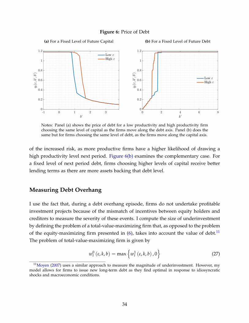
Figure 6: Price of Debt

(a) For a Fixed Level of Future Capital (b) For a Fixed Level of Future Debt

Notes: Panel (a) shows the price of debt for a low productivity and high productivity firmchoosing the same level of capital as the firms move along the debt axis. Panel (b) does thesame but for firms choosing the same level of debt, as the firms move along the capital axis.

of the increased risk, as more productive firms have a higher likelihood of drawing ahigh productivity level next period. Figure 6(b) examines the complementary case. Fora fixed level of next period debt, firms choosing higher levels of capital receive betterlending terms as there are more assets backing that debt level.

Measuring Debt Overhang

I use the fact that, during a debt overhang episode, firms do not undertake profitableinvestment projects because of the mismatch of incentives between equity holders andcreditors to measure the severity of these events. I compute the size of underinvestmentby defining the problem of a total-value-maximizing firm that, as opposed to the problemof the equity-maximizing firm presented in (6), takes into account the value of debt.11

The problem of total-value-maximizing firm is given by

w0t (ε, k, b) = max

{w1

t (ε, k, b) , 0}

(27)

11Moyen (2007) uses a similar approach to measure the magnitude of underinvestment. However, mymodel allows for firms to issue new long-term debt as they find optimal in response to idiosyncraticshocks and macroeconomic conditions.

34

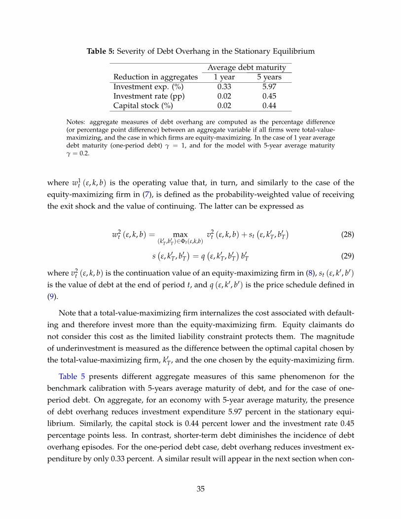
Table 5: Severity of Debt Overhang in the Stationary Equilibrium

Average debt maturityReduction in aggregates 1 year 5 yearsInvestment exp. (%) 0.33 5.97Investment rate (pp) 0.02 0.45Capital stock (%) 0.02 0.44

Notes: aggregate measures of debt overhang are computed as the percentage difference(or percentage point difference) between an aggregate variable if all firms were total-value-maximizing, and the case in which firms are equity-maximizing. In the case of 1 year averagedebt maturity (one-period debt) γ = 1, and for the model with 5-year average maturityγ = 0.2.

where w1t (ε, k, b) is the operating value that, in turn, and similarly to the case of the

equity-maximizing firm in (7), is defined as the probability-weighted value of receivingthe exit shock and the value of continuing. The latter can be expressed as

w2t (ε, k, b) = max

(k′T ,b′T)∈Φt(ε,k,b)v2

t (ε, k, b) + st(ε, k′T, b′T

)(28)

s(ε, k′T, b′T

)= q

(ε, k′T, b′T

)b′T (29)

where v2t (ε, k, b) is the continuation value of an equity-maximizing firm in (8), st (ε, k′, b′)

is the value of debt at the end of period t, and q (ε, k′, b′) is the price schedule defined in(9).

Note that a total-value-maximizing firm internalizes the cost associated with default-ing and therefore invest more than the equity-maximizing firm. Equity claimants donot consider this cost as the limited liability constraint protects them. The magnitudeof underinvestment is measured as the difference between the optimal capital chosen bythe total-value-maximizing firm, k′T, and the one chosen by the equity-maximizing firm.

Table 5 presents different aggregate measures of this same phenomenon for thebenchmark calibration with 5-years average maturity of debt, and for the case of one-period debt. On aggregate, for an economy with 5-year average maturity, the presenceof debt overhang reduces investment expenditure 5.97 percent in the stationary equi-librium. Similarly, the capital stock is 0.44 percent lower and the investment rate 0.45percentage points less. In contrast, shorter-term debt diminishes the incidence of debtoverhang episodes. For the one-period debt case, debt overhang reduces investment ex-penditure by only 0.33 percent. A similar result will appear in the next section when con-

35

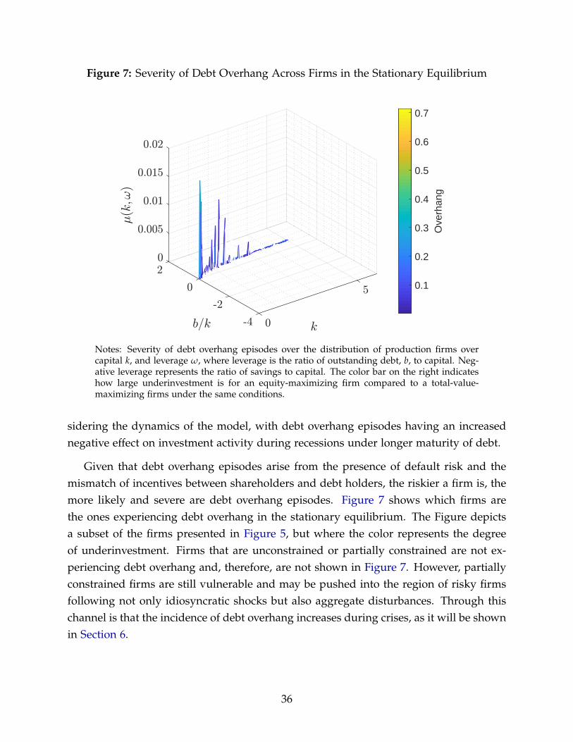
Figure 7: Severity of Debt Overhang Across Firms in the Stationary Equilibrium

0.1

0.2

0.3

0.4

0.5

0.6

0.7

Ove

rhan

g

Notes: Severity of debt overhang episodes over the distribution of production firms overcapital k, and leverage ω, where leverage is the ratio of outstanding debt, b, to capital. Neg-ative leverage represents the ratio of savings to capital. The color bar on the right indicateshow large underinvestment is for an equity-maximizing firm compared to a total-value-maximizing firms under the same conditions.

sidering the dynamics of the model, with debt overhang episodes having an increasednegative effect on investment activity during recessions under longer maturity of debt.

Given that debt overhang episodes arise from the presence of default risk and themismatch of incentives between shareholders and debt holders, the riskier a firm is, themore likely and severe are debt overhang episodes. Figure 7 shows which firms arethe ones experiencing debt overhang in the stationary equilibrium. The Figure depictsa subset of the firms presented in Figure 5, but where the color represents the degreeof underinvestment. Firms that are unconstrained or partially constrained are not ex-periencing debt overhang and, therefore, are not shown in Figure 7. However, partiallyconstrained firms are still vulnerable and may be pushed into the region of risky firmsfollowing not only idiosyncratic shocks but also aggregate disturbances. Through thischannel is that the incidence of debt overhang increases during crises, as it will be shownin Section 6.

36

6 Understanding the Great Recession

I now analyze the importance of each one of the model mechanisms to explain thedynamics of investment during the Great Recession. Focusing on perfect foresight re-sponses, in Subsection 6.1 I first show the implications arising from having long-termfinancing and nominal debt in a partial equilibrium context. Then, Subsection 6.2 con-siders the price effects in the transmission of real and financial shocks, and evaluates inwhat extent the model captures the unusual investment dynamics observed during the2007 episode.

6.1 Dynamics Under Fixed Prices

To have a first approximation to the relevance of accounting for firms’ long-term debt po-sitions, I simulate a large panel of firms using the solution of the model presented aboveat the stationary equilibrium. Table 6 presents the correlation of several model variablesfor two different values of average debt maturity: five years, as in the benchmark calibra-tion and one year, as in a model with short-term debt. The importance of idiosyncraticproductivity and capital in determining firms’ choices falls when including multi-periodfinancing. For example, the correlation between individual productivity and investmentrates falls from 0.43 to 0.35 when moving from a model of short-term debt to one oflong-term debt. Conversely, the incidence of debt is larger with multi-period debt. Thecorrelation of leverage and output is 0.22 in the model with long-term debt and nearlyhalf for the case short-term debt. The relationship between investment rates and lever-age is also stronger, with a correlation 3.5 points higher (in absolute value) in the modelwith multi-period debt.

What does this result imply for the transmission of real and financial shocks? Tostart addressing this question, I begin with a series of fixed prices experiments designedto gauge the relevance of accounting for long-maturity debt to explain the Great Re-cession. Figures 8 and 9 summarize the perfect foresight partial equilibrium responseof the multi-period-debt economy to a persistent shock to the total factor productivityand a persistent negative financial shock. For each shock, I consider two different casesof average debt maturity. The financial shock increases the financial costs of operation,ξm,t (ε), in 0.75 percent of the value of the efficient level of output.12 These responses as-

12The efficient output level, y∗ (ε), is obtained by a firm that is not subject to financial frictions and that,hence, can implement the frictionless level of capital, k∗ (ε).

37

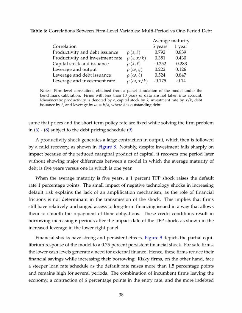
Table 6: Correlations Between Firm-Level Variables: Multi-Period vs One-Period Debt

Average maturityCorrelation 5 years 1 yearProductivity and debt issuance ρ (ε, `) 0.792 0.839Productivity and investment rate ρ (ε, x/k) 0.351 0.430Capital stock and issuance ρ (k, `) -0.252 -0.283Leverage and output ρ (ω, y) 0.222 0.126Leverage and debt issuance ρ (ω, `) 0.524 0.847Leverage and investment rate ρ (ω, x/k) -0.175 -0.14

Notes: Firm-level correlations obtained from a panel simulation of the model under thebenchmark calibration. Firms with less than 10 years of data are not taken into account.Idiosyncratic productivity is denoted by ε, capital stock by k, investment rate by x/k, debtissuance by `, and leverage by ω = b/k, where b is outstanding debt.

sume that prices and the short-term policy rate are fixed while solving the firm problemin (6) - (8) subject to the debt pricing schedule (9).

A productivity shock generates a large contraction in output, which then is followedby a mild recovery, as shown in Figure 8. Notably, despite investment falls sharply onimpact because of the reduced marginal product of capital, it recovers one period laterwithout showing major differences between a model in which the average maturity ofdebt is five years versus one in which is one year.

When the average maturity is five years, a 1 percent TFP shock raises the defaultrate 1 percentage points. The small impact of negative technology shocks in increasingdefault risk explains the lack of an amplification mechanism, as the role of financialfrictions is not determinant in the transmission of the shock. This implies that firmsstill have relatively unchanged access to long-term financing issued in a way that allowsthem to smooth the repayment of their obligations. These credit conditions result inborrowing increasing 6 periods after the impact date of the TFP shock, as shown in theincreased leverage in the lower right panel.

Financial shocks have strong and persistent effects. Figure 9 depicts the partial equi-librium response of the model to a 0.75-percent persistent financial shock. For safe firms,the lower cash levels generate a need for external finance. Hence, these firms reduce theirfinancial savings while increasing their borrowing. Risky firms, on the other hand, facea steeper loan rate schedule as the default rate raises more than 1.5 percentage pointsand remains high for several periods. The combination of incumbent firms leaving theeconomy, a contraction of 6 percentage points in the entry rate, and the more indebted

38

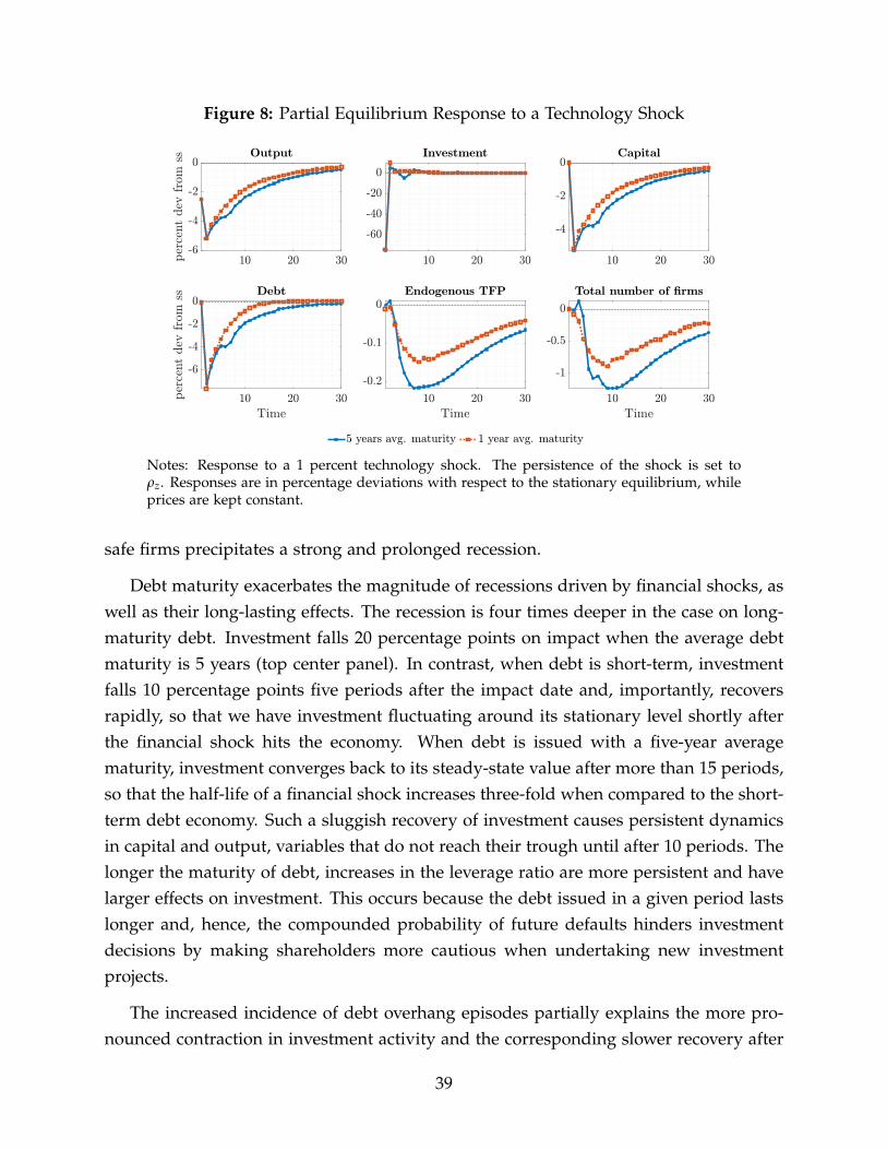
Figure 8: Partial Equilibrium Response to a Technology Shock

Notes: Response to a 1 percent technology shock. The persistence of the shock is set toρz. Responses are in percentage deviations with respect to the stationary equilibrium, whileprices are kept constant.

safe firms precipitates a strong and prolonged recession.

Debt maturity exacerbates the magnitude of recessions driven by financial shocks, aswell as their long-lasting effects. The recession is four times deeper in the case on long-maturity debt. Investment falls 20 percentage points on impact when the average debtmaturity is 5 years (top center panel). In contrast, when debt is short-term, investmentfalls 10 percentage points five periods after the impact date and, importantly, recoversrapidly, so that we have investment fluctuating around its stationary level shortly afterthe financial shock hits the economy. When debt is issued with a five-year averagematurity, investment converges back to its steady-state value after more than 15 periods,so that the half-life of a financial shock increases three-fold when compared to the short-term debt economy. Such a sluggish recovery of investment causes persistent dynamicsin capital and output, variables that do not reach their trough until after 10 periods. Thelonger the maturity of debt, increases in the leverage ratio are more persistent and havelarger effects on investment. This occurs because the debt issued in a given period lastslonger and, hence, the compounded probability of future defaults hinders investmentdecisions by making shareholders more cautious when undertaking new investmentprojects.

The increased incidence of debt overhang episodes partially explains the more pro-nounced contraction in investment activity and the corresponding slower recovery after

39

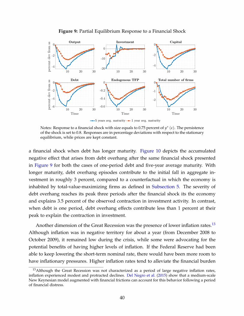
Figure 9: Partial Equilibrium Response to a Financial Shock

Notes: Response to a financial shock with size equals to 0.75 percent of y∗ (ε). The persistenceof the shock is set to 0.8. Responses are in percentage deviations with respect to the stationaryequilibrium, while prices are kept constant.

a financial shock when debt has longer maturity. Figure 10 depicts the accumulatednegative effect that arises from debt overhang after the same financial shock presentedin Figure 9 for both the cases of one-period debt and five-year average maturity. Withlonger maturity, debt overhang episodes contribute to the initial fall in aggregate in-vestment in roughly 3 percent, compared to a counterfactual in which the economy isinhabited by total-value-maximizing firms as defined in Subsection 5. The severity ofdebt overhang reaches its peak three periods after the financial shock its the economyand explains 3.5 percent of the observed contraction in investment activity. In contrast,when debt is one period, debt overhang effects contribute less than 1 percent at theirpeak to explain the contraction in investment.

Another dimension of the Great Recession was the presence of lower inflation rates.13

Although inflation was in negative territory for about a year (from December 2008 toOctober 2009), it remained low during the crisis, while some were advocating for thepotential benefits of having higher levels of inflation. If the Federal Reserve had beenable to keep lowering the short-term nominal rate, there would have been more room tohave inflationary pressures. Higher inflation rates tend to alleviate the financial burden

13Although the Great Recession was not characterized as a period of large negative inflation rates,inflation experienced modest and protracted declines. Del Negro et al. (2015) show that a medium-scaleNew Keynesian model augmented with financial frictions can account for this behavior following a periodof financial distress.

40

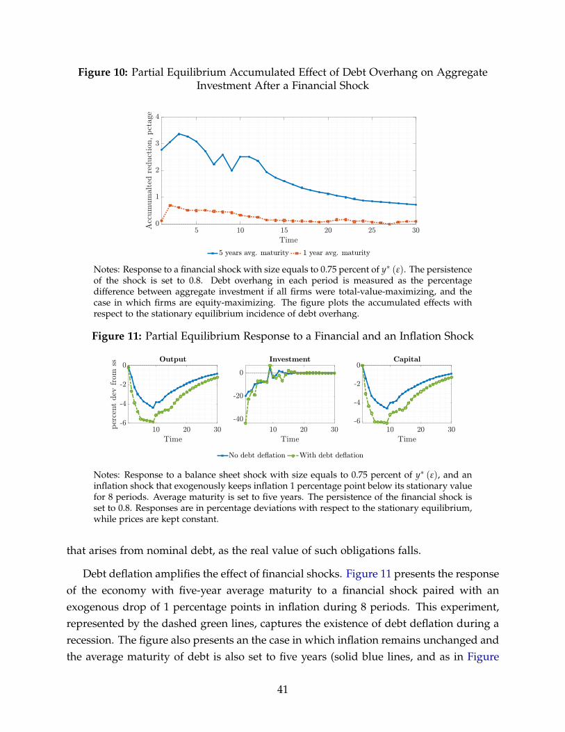
Figure 10: Partial Equilibrium Accumulated Effect of Debt Overhang on AggregateInvestment After a Financial Shock

Notes: Response to a financial shock with size equals to 0.75 percent of y∗ (ε). The persistenceof the shock is set to 0.8. Debt overhang in each period is measured as the percentagedifference between aggregate investment if all firms were total-value-maximizing, and thecase in which firms are equity-maximizing. The figure plots the accumulated effects withrespect to the stationary equilibrium incidence of debt overhang.

Figure 11: Partial Equilibrium Response to a Financial and an Inflation Shock

Notes: Response to a balance sheet shock with size equals to 0.75 percent of y∗ (ε), and aninflation shock that exogenously keeps inflation 1 percentage point below its stationary valuefor 8 periods. Average maturity is set to five years. The persistence of the financial shock isset to 0.8. Responses are in percentage deviations with respect to the stationary equilibrium,while prices are kept constant.

that arises from nominal debt, as the real value of such obligations falls.

Debt deflation amplifies the effect of financial shocks. Figure 11 presents the responseof the economy with five-year average maturity to a financial shock paired with anexogenous drop of 1 percentage points in inflation during 8 periods. This experiment,represented by the dashed green lines, captures the existence of debt deflation during arecession. The figure also presents an the case in which inflation remains unchanged andthe average maturity of debt is also set to five years (solid blue lines, and as in Figure

41

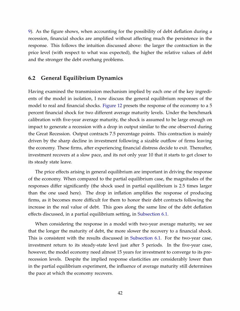
9). As the figure shows, when accounting for the possibility of debt deflation during arecession, financial shocks are amplified without affecting much the persistence in theresponse. This follows the intuition discussed above: the larger the contraction in theprice level (with respect to what was expected), the higher the relative values of debtand the stronger the debt overhang problems.

6.2 General Equilibrium Dynamics

Having examined the transmission mechanism implied by each one of the key ingredi-ents of the model in isolation, I now discuss the general equilibrium responses of themodel to real and financial shocks. Figure 12 presets the response of the economy to a 5percent financial shock for two different average maturity levels. Under the benchmarkcalibration with five-year average maturity, the shock is assumed to be large enough onimpact to generate a recession with a drop in output similar to the one observed duringthe Great Recession. Output contracts 7.5 percentage points. This contraction is mainlydriven by the sharp decline in investment following a sizable outflow of firms leavingthe economy. These firms, after experiencing financial distress decide to exit. Thereafter,investment recovers at a slow pace, and its not only year 10 that it starts to get closer toits steady state leave.

The price effects arising in general equilibrium are important in driving the responseof the economy. When compared to the partial equilibrium case, the magnitudes of theresponses differ significantly (the shock used in partial equilibrium is 2.5 times largerthan the one used here). The drop in inflation amplifies the response of producingfirms, as it becomes more difficult for them to honor their debt contracts following theincrease in the real value of debt. This goes along the same line of the debt deflationeffects discussed, in a partial equilibrium setting, in Subsection 6.1.

When considering the response in a model with two-year average maturity, we seethat the longer the maturity of debt, the more slower the recovery to a financial shock.This is consistent with the results discussed in Subsection 6.1. For the two-year case,investment return to its steady-state level just after 5 periods. In the five-year case,however, the model economy need almost 15 years for investment to converge to its pre-recession levels. Despite the implied response elasticities are considerably lower thanin the partial equilibrium experiment, the influence of average maturity still determinesthe pace at which the economy recovers.

42

Figu

re12

:Gen

eral

Equi

libri

umR

espo

nse

toa

Fina

ncia

lSho

ck

510

1520

Tim

e

-0.2

-0.1

5

-0.1

-0.0

50

Percentchange

Outp

ut

5ye

arsav

g.m

aturity

1ye

arav

g.m

aturity

510

1520

Tim

e

-0.4

-0.3

-0.2

-0.10

Percentchange

Consu

mpti

on

510

1520

Tim

e

-1.5-1

-0.50

0.5

Percentchange

Invest

ment

510

1520

Tim

e

-0.4

-0.3

-0.2

-0.10

0.1

Percentchange

Capit

al

510

1520

Tim

e

-0.2

-0.10

0.1

0.2

Percentchange

Labor

510

1520

Tim

e

-0.2

5

-0.2

-0.1

5

-0.1

-0.0

50

Percentchange

Endogenous

TF

P

510

1520

Tim

e

-5051015

Percentchange

Debt

510

1520

Tim

e

01234

Percentagept.change

Gro

ssle

vera

ge

510

1520

Tim

e

0

0.050.1

0.150.2

Percentagept.change

In.ati

on

510

1520

Tim

e

-0.3

-0.2

-0.10

0.1

0.2

Percentchange

Marg

inalcost

s

510

1520

Tim

e

6.2

6.256.3

6.356.4

6.45

Percentage

Nom

inalin

tere

stra

te

510

1520

Tim

e

-0.8

-0.6

-0.4

-0.20

Percentagept.change

Ris

kfr

ee

long-t

erm

Not

es:

Res

pons

eto

afin

anci

alsh

ock

wit

hsi

zeeq

uals

to5

perc

ent

ofy∗

(ε).

The

pers

iste

nce

ofth

esh

ock

isse

tto

0.9,

and

its

size

isch

osen

toge

nera

tea

cont

ract

ion

ofar

ound

4pe

rcen

tin

outp

ut.R

espo

nses

are

inpe

rcen

tage

devi

atio

nsw

ith

resp

ectt

oth

est

atio

nary

equi

libri

um.

43

7 Concluding Remarks

In this paper, I explored the reasons behind the unusually slow recovery of investmentfollowing the Great Recession. I presented empirical evidence suggesting that firmswith large financial burden arising from previously issued debt experience larger con-tractions in their investment expenditure. Importantly, this form of financial distresswas more prevalent during the 2007 recession. I then presented a quantitative stochasticgeneral equilibrium model to examine the mechanisms underlying the empirical results.Critically, the quantitative framework stresses the importance of accounting for the inter-action between the debt maturity structure across heterogeneous firms and the bindingzero constraint for monetary policy. To obtain these results, the model incorporates newelements, namely, nominal and defaultable long-term financing in an New Keynesianmodel with heterogeneous firms, and a quantitative strategy that allows me to considerlarge shocks and the zero lower bound simultaneously. I used this framework to showthat firms with large debt positions at the onset of large recession are more likely to expe-rience debt overhang episodes. Using the model, I showed that debt overhang episodesnot only lower investment during normal times, but also make more severe the con-traction in investment expenditure following a financial shock, and slower the recovery.Importantly, the severity of these episodes increases when accounting for debt deflationeffects. .

References

Almeida, Heitor, Murillo Campello, Bruno Laranjeira, and Scott Weisbenner, “Cor-porate Debt Maturity and the Real Effects of the 2007 Credit Crisis,” Critical FinanceReview, 2011, 1, 3–58.

Arellano, Cristina, Yan Bai, and Patrick J. Kehoe, “Financial Frictions and Fluctuationsin Volatility,” 2018. Manuscript.

Auclert, Adrien, “Monetary Policy and the Redistribution Channel,” 2017. Manuscript,Stanford University.

Bernanke, Ben S., “Opening Remarks: Monetary Policy Since the Onset of the Crisis,”in “Proceedings: Economic Policy Symposium Jackson Hole” 2012.

44

Christiano, Lawrence J., Martin S. Eichenbaum, and Mathias Trabandt, “Understand-ing the Great Recession,” American Economic Journal: Macroeconomics, 2015, 7 (1), 110–167.

Crouzet, Nicolas, “Default, Debt Maturity and Investment Dynamics,” 2017.Manuscript, Kellogg School of Management, Northwestern University.

and Neil R. Mehrotra, “Small and Large Firms Over the Business Cycle,” 2018.Manuscript, Kellogg School of Management, Northwestern University.

Del Negro, Marco, Marc P. Giannoni, and Frank Schorfheide, “Inflation in the GreatRecession and New Keynesian Models,” American Economic Journal: Macroeconomics,2015, 7 (1), 168–196.

Dinlersoz, Emin, Sebnem Kalemli-Ozcan, Henry Hyatt, and Veronika Penciakova,“Leverage Over the Life Cycle and Implications for Firm Growth and Shock Respon-siveness,” Technical Report 25226, NBER Working Paper 2018.

Eggertsson, Gauti and Michael Woodford, “The Zero Bound on Interest Rates and Op-timal Monetary Policy,” Brookings Papers on Economic Activity, 2003, (1).

Erickson, Timothy and Toni M. Whited, “Measurement Error and the Relationshipbetween Investment and q,” Journal of Political Economy, 2000, 108 (5), 1027–1057.

Fazzari, Steven M., R. Glenn Hubbard, and Bruce C. Petersen, “Financing Constraintsand Corporate Investment,” Brookings Papers on Economic Activity, 1988, 1988 (1), 141–206.

Fernández-Villaverde, Jesús, Grey Gordon, Pablo Guerrón-Quintana, and Juan F.Rubio-Ramírez, “Nonlinear Adventures at the Zero Lower Bound,” Journal of Eco-nomic Dynamics and Control, 2015, 57, 182–204.

Gilchrist, Simon and Egon Zakrajšek, “Credit Spreads and Business Cycle Fluctua-tions,” American Economic Review, 2012, 102 (4), 1692–1720.

Gomes, Joao F., “Financing Investment,” American Economic Review, 2001, 91 (5), 1263–1285.

, Urban Jermann, and Lukas Schmid, “Sticky Leverage,” American Economic Review,2016, 106 (12), 3800–3828.

45

Guedes, Jose and Tim Opler, “The Determinants of the Maturity of Corporate DebtIssues,” Journal of Finance, 1996, 51 (5), 1809–1833.

Hayashi, Fumio, “Tobin’s Marginal q and Average q: A Neoclassical Interpretation,”Econometrica, 1982, 50 (1), 213–224.

Hennessy, Christopher A., “Tobin’s Q, Debt Overhang, and Investment,” Journal of Fi-nance, 2004, 59 (4), 1717–1742.

, Amnon Levy, and Toni M. Whited, “Testing Q Theory with Financing Frictions,”Journal of Financial Economics, 2007, 83 (3), 691–717.

Jeenas, Priit, “Firm Balance Sheet Liquidity, Monetary Policy Shocks, and InvestmentDynamics,” 2019. Manuscript.

Jungherr, Joachim and Immo Schott, “Slow Debt , Deep Recessions,” 2019. Manuscript.

and , “Optimal Debt Maturity and Firm Investment,” 2020. Manuscript.

Kalemli-Ozcan, Sebnem, Luc Laeven, and David Moreno, “Debt Overhang, RolloverRisk, and Corporate Investment: Evidence from the European Crisis,” Technical Re-port 24555, NBER Working Paper 2018.

Kaplan, Greg, Benjamin Moll, and Giovanni L. Violante, “Monetary Policy Accordingto HANK,” American Economic Review, 2018, 108 (3), 697–743.

Khan, Aubhik and Julia K. Thomas, “Credit Shocks and Aggregate Fluctuations in anEconomy with Production Heterogeneity,” Journal of Political Economy, 2013, 121 (6),1055–1107.

, Tatsuro Senga, and Julia K. Thomas, “Default Risk and Aggregate Fluctuations in anEconomy with Production Heterogeneity,” 2016. Manuscript, Ohio State University.

Lakdawala, Aeimit and Timothy Moreland, “Monetary Policy and Firm Heterogeneity:The Role of Leverage Since the Financial Crisis,” 2019. Manuscript, Michigan StateUniversity.

Lucas, Robert E. Jr. and Edward C. Prescott, “Investment Under Uncertainty,” Econo-metrica, 1971, 39 (5), 659–681.

Mckay, Alisdair, Emi Nakamura, and Jón Steinsson, “The Power of Forward GuidanceRevisited,” American Economic Review, 2016, 106 (10), 3133–3158.

46

Moyen, Nathalie, “How Big is the Debt Overhang Problem?,” Journal of Economic Dy-namics and Control, 2007, 31 (2), 433–472.

Myers, Stewart, “Determinants of Corporate Borrowing,” Journal of Financial Economics,1977, 5, 147–175.

Negro, Marco Del, Gauti Eggertsson, Andrea Ferrero, and Nobuhiro Kiyotaki, “TheGreat Escape? A Quantitative Evaluation of the Fed’s Liquidity Facilities,” AmericanEconomic Review, 2017, 107 (3), 824–857.

Ottonello, Pablo and Thomas Winberry, “Financial Heterogeneity and the InvestmentChannel of Monetary Policy,” 2018. Manuscript, University of Chicago Booth Schoolof Business.

Poeschl, Johannes, “Corporate Debt Maturity and Investment over the Business Cycle,”2018. Working Paper No. 125, Danmarks Nationalbank.

Whited, Toni M. and Guojun Wu, “Financial Constraints Risk,” Review of Financial Stud-ies, 2006, 19 (2), 531–559.

Wong, Arlene, “Population Aging and the Transmission of Monetary Policy to Con-sumption and Population Aging,” 2018. Manuscript, Princeton Univeristy.

Zetlin-Jones, Ariel and Ali Shourideh, “External Financing and the Role of FinancialFrictions Over the Business Cycle: Measurement and Theory,” Journal of MonetaryEconomics, 2017, 92, 1–15.

47

A Data

A.1 Flow of Funds

The Statistical Release Z.1, Financial Accounts of the United States, is published bythe Federal Reserve Board. It includes flow of funds, balance sheet, and integratedmacroeconomic account data. It reports data on transaction and levels of financial assetsand liabilities for, among others, nonfinancial corporate and noncorporate businesses,by sector and financial instrument. This data is at a quarterly frequency and comprisesthe period 1951Q4 - 2017Q3.

I use quarterly data seasonally adjusted annual rates covering nonfinancial corporatebusiness. Total debt (Table B.103) is defined as the sum of debt in securities (FL104122005.Q)and loans (FL104123005.Q). Leverage (Table B.103) is total debt divided by total assets(FL102000005.Q). Total long-term debt (Table L.103) is computed as the sum of munic-ipal securities (FL103162000.Q), corporate bonds (FL103163003.Q), and total mortgages(FL103165005.Q). Total short-term debt is total debt minus total long-term debt. LT debtratio is (Table L.103) constructed as: 100 minus short-term debt as a percentage of totaldebt (FL104140006.Q). I deflate all nominal variables using the Consumer Price Index forAll Urban Consumers from Fred (CPIAUCSL).

A.2 Compustat

The empirical analysis uses firm-level data from the Fundamentals Quarterly datasetfrom Compustat for the period 1984Q1 to 2017Q4. The construction of the variablesfollows standard practices in the literature of firm investment and corporate finance.

Starting with Compustat Fundamentals Annual, I apply several filters to this data.First, I drop observations for utilities (SIC codes between 4900 and 4999), financial in-stitutions (SICS codes 6000 to 6799), public administrations (SIC codes 9100 to 9799),ADRs (SIC code 8880), and foreign governments (SIC code 8888). I also delete firms notincorporated in the U.S. (fic code different from USA). Regarding financial variables, Ieliminate firm-year observations with acquisitions (aqc) larger than 5% percent of as-sets (at); firms with missing or negative values for total assets (at), capital expenditures(capx), property, plant, and equipment (ppegt), cash holdings (che), or sales (sale); firmsfor which cash holdings (che), capital expenditures (capx) or property, plant and equip-

48

ment (ppent) are larger than total assets (at); firms for which the value of total assets (at)is less than $0.5 million; and firms displaying asset growth or sales growth exceeding100%.

When using annual data, the main measure of investment used int the paper ∆ log ki,t+1

is constructed as the log difference between property, plant and equipment (ppegt) andits lagged value. The alternative measure used for robustness exercises, (xi,t/ki,t), is com-puted as the ratio of capital expenditures (capx) to the lagged value of property plantand equipment (ppegt). For quarterly data, given that the gross value of property, plantand equipment (ppentq) is so sparsely populated, I follow Ottonello and Winberry (2018)and construct ki,t by adding the changes in net property, plant and equipment (ppentq)on top of the firms observation for each firm with non missing value for ppentq.

As is standard in the literature, all debt issued with maturity above one year is con-sidered long-term. In the annual database, dollar amounts of long-term debt maturingin between 1 and five or more years after the annual report are denoted by dd1 to dd5.Debt maturing in more than one year is denoted by dltt. Consequently, I drop firmswith total long-term debt (dd1+dltt) greater than total assets (at), and firms for whichdebt maturing in more than one year (dltt) is lower than the sum of debt maturingin two, three, four, and five years (dd2+dd3+dd4+dd5). Finally, I keep observations withnon-missing values in all variables used and winsorize at the 0.1% to eliminate outliers.

Total debt is the sum of debt in current liabilities (dlc) and total long-term debtmaturing in more than 1 year (dltt). Firm leverage is computed as the ratio of total debtto total assets (at). The long-term debt ratio is total long-term debt (dd1+dltt) dividedby total debt. The fraction of total debt maturing within the next year is computed asdebt in current liabilities (dlc) divided by total debt. The fraction of long-term debtmaturing within the next year is computed as dd1 divided by total long-term debt.

As for control variables, cash flow is defined as the ratio of net income (ib) plusdepreciation and amortization (dp) to the lag of quarterly property, plant and equipment(ppegt). Tobin’s q is the ratio of total assets (at) plus market capitalization (prcc×csho)minus common equity (ceq) minus deferred taxes and investment tax credit (txditc), tototal assets (at). Size is proxied by the log of total asset (at).

Finally, sectors are defined as follows: Agriculture, forestry and fishing (SIC code0100-0999), Mining (1000-1499), Construction (1500-1799), Manufacturing (2000-3999),Transportation, communications, electric, gas and sanitary services (4000-4999), Whole-sale trade (5000-5199) Retail trade (5200-5999), and Services (7000-8999).

49

B Reduced-Form Model of Firm Investment

Consider the decision-theoretic problem of a firm that optimally chooses investment andhow to finance that expenditure with debt. Time is discrete and infinite. The firm carriesout production using a decreasing return to scale technology: y = εkα, where ε is aproductivity shock that follows a Markov process and k is the capital stock owned bythe firm and α (0, 1). When adjusting their capital stock, the firm is subject to adjustmentcosts Ψ (k, k′). The adjustment cost function satisfies Ψ2 > 0 and Ψ22 > 0.

To finance investment expenditure, the firm can issue a long-term defaultable bondb ∈ [0, ∞). Each period, each bond is amortized at the rate γ, and pays a coupon κ.p (ε, k′, b′) denotes the price of firm debt. I assume that pk′ ≥ 0 and pb′ ≤ 0. Theseassumptions are a useful form of capturing the effects of default risk on interest rates inan reduce form manner. Implicitly, they mean that, as the firm increases it capital stock,the expected output next period will be higher; and as the firm has less debt, the morelikely is for it to be able to repay. Finally, I further assume that the firm cannot save. Thefirm maximizes its value:

v (ε, k, b) = maxk,b

[D(ε, k, b, k′, b′

)+ βEv

(ε′k′, b′

)](30)

where dividends are given by

D(ε, k, b, k′, b′

)= εkα − (κ + γ) b + (1− δ) k− k′ −Ψ

(k, k′

)+ p

(k′, b′

)` (31)

and where debt issuance ` is` = b′ − (1− γ) b (32)

The optimality condition for capital is given by

1 + Ψ2(k, k′

)= pk′

[b′ − (1− γ) b

]+ βED1v

(ε′, k′, b′

)(33)

The left-hand side of the condition captures the marginal cost of investment, whichincludes the price per unit of k′ and the associated adjustment costs. On the right-handside, we have the marginal benefit of investment, which is the sum of the marginalrevenue for a fixed level of debt issuance and the marginal shadow value of capital.From the envelope condition, this shadow value is the marginal return on capital, next

50

of adjustment costD1v (ε, k, b) = αεkα−1 + (1− δ)−Ψ1

(k, k′

)(34)

The optimality condition for debt is

pb′[b′ − (1− γ) b

]+ p = −βD2Ev

(ε′k′, b′

)(35)

In this condition, the left-hand side is the marginal revenue from issuing more debt. Ittakes into account change in p (negative), and the extra resources p per unit of `. On theright-hand side we have the marginal cost of increasing debt, noting that D2v (ε, k, b) < 0as the envelope condition for debt is

D2 (ε, k, b) = − (κ + γ)− p (1− γ) (36)

Then, the marginal cost of increasing debt is the sum of payments in coupon and thefraction γ of the principal, plus the cost of debt (valued at p) that has not yet matured.Combining (33) and (35) yields14

1 + Ψ2(k, k′

)= pk′

1pb′{β [(κ + γ) + p (1− γ)]− p}

+ βE[αε′(k′)α−1

+ (1− δ)−Ψ1(k′, k′′

)](37)

Now, I derive an investment equation that will be used to motivate the empiricalspecification in Section 2. Define the shadow value of capital as

q (ε, k, b) = βED1v(ε′, k′, b′

)(38)

Therefore, equation (37) can be rewritten as

1 + Ψ2(k, k′

)= pk′

1pb′{β [(κ + γ) + p (1− γ)]− p}+ q (ε, k, b)

Since the first partials derivatives of Ψ are homogeneous of degree 0, and as Ψ2 is

14Note that, in absence of default risk, the price of debt is p = β (κ + γ) / [1− β (1− γ)] and, hence, thecondition (37) becomes

1 + Ψ2(k, k′

)= βE

[αε′(k′)α−1

+ (1− δ)−Ψ1(k′, k′′

)]This is the frictionless optimality condition for capital in a neoclassical model of investment.

51

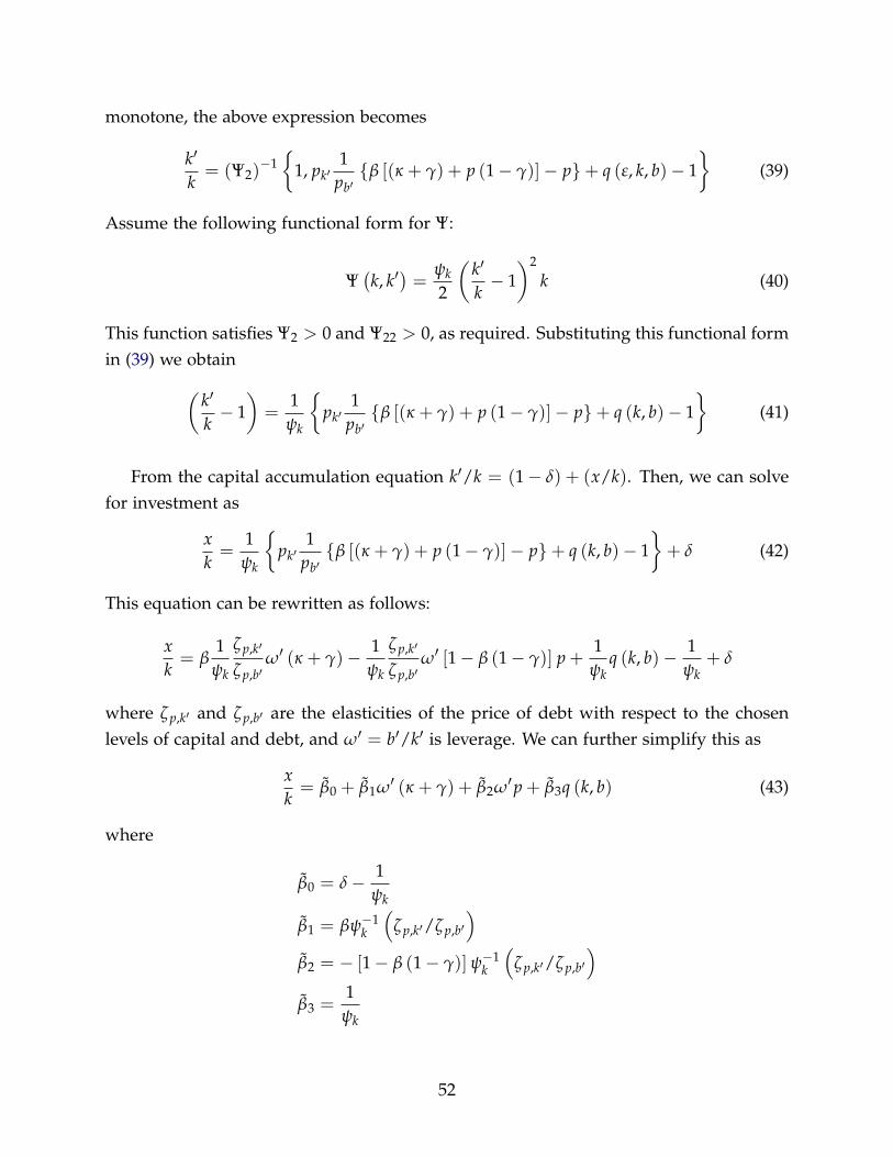
monotone, the above expression becomes

k′

k= (Ψ2)

−1{

1, pk′1

pb′{β [(κ + γ) + p (1− γ)]− p}+ q (ε, k, b)− 1

}(39)

Assume the following functional form for Ψ:

Ψ(k, k′

)=

ψk2

(k′

k− 1)2

k (40)

This function satisfies Ψ2 > 0 and Ψ22 > 0, as required. Substituting this functional formin (39) we obtain(

k′

k− 1)=

1ψk

{pk′

1pb′{β [(κ + γ) + p (1− γ)]− p}+ q (k, b)− 1

}(41)

From the capital accumulation equation k′/k = (1− δ) + (x/k). Then, we can solvefor investment as

xk=

1ψk

{pk′

1pb′{β [(κ + γ) + p (1− γ)]− p}+ q (k, b)− 1

}+ δ (42)

This equation can be rewritten as follows:

xk= β

1ψk

ζp,k′

ζp,b′ω′ (κ + γ)− 1

ψk

ζp,k′

ζp,b′ω′ [1− β (1− γ)] p +

1ψk

q (k, b)− 1ψk

+ δ

where ζp,k′ and ζp,b′ are the elasticities of the price of debt with respect to the chosenlevels of capital and debt, and ω′ = b′/k′ is leverage. We can further simplify this as

xk= β0 + β1ω′ (κ + γ) + β2ω′p + β3q (k, b) (43)

where

β0 = δ− 1ψk

β1 = βψ−1k

(ζp,k′/ζp,b′

)β2 = − [1− β (1− γ)]ψ−1

k

(ζp,k′/ζp,b′

)β3 =

1ψk

52

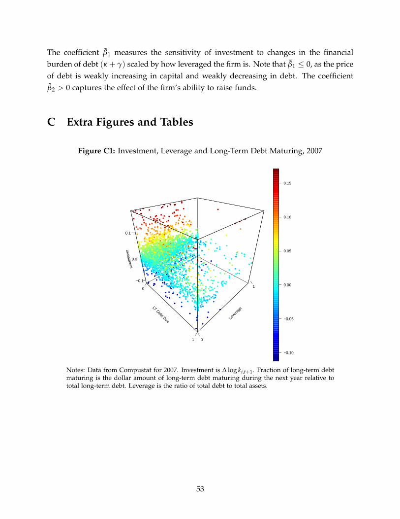
The coefficient β1 measures the sensitivity of investment to changes in the financialburden of debt (κ + γ) scaled by how leveraged the firm is. Note that β1 ≤ 0, as the priceof debt is weakly increasing in capital and weakly decreasing in debt. The coefficientβ2 > 0 captures the effect of the firm’s ability to raise funds.

C Extra Figures and Tables

Figure C1: Investment, Leverage and Long-Term Debt Maturing, 2007

LT Debt Due

0

1

Leve

rage

0

1

Investment

−0.1

0.0

0.1

●●

●●●●●

●●

●

●●

●

●●

●

●

●●

●●

● ●

●●●●

●

●

●

●

●

●●

●●●

●●

●

●

●

●

●

●

●

●

●●

●●

●●

●

●● ●

●

●

●●●

●

●

●

●

●

●

●

●

●

●

●

●

●

●●

●

●

●

●

●

●

●

●

●

●

●●

●

●●

●

●

●

● ●

●

●

●●

●

● ●

●

●●

●

●

●

●

●

●

●●

●●

●

●

●

●

●

●

●

●

●

●

●

●

●

●●

●●

●

●

●

●

●

●●

●

●

●

●

●

●

●●

●

●

● ●

●

●●

●●

●

●

●

●●

●

●

●

●

●

●

●●

●

●

●

●●●

●

●

●

●

●●

●

●●

●

●

●

●●

●

●

●

●

●

●

●●●

●

●

●

●

●

●

●

●

●

●

●

●

●

●

●

●

●

●

●

●

●

●

●

●

●

●

●

●●

●

●

●

●

●

●●

●

●

●●

●

●

●

●

●

●

●●

●

●

●

●

●

●

●

●

●●

●

●

●

●

●

●

●

●

●

●

●

●

●

●

●

●

●

●

●

●

●

●

●●

●

●●

●

●

● ●

●●

●

●

●

●●●●

●●

●

●

● ●

●

●

●

●

●

●●

●●

●●

●

●

●

●

●

●

●

●

●

●

●

●

●

●

●

●●●

●

●

●

●

●

●

●

●

●

●●● ●●

●

●

●●

●

●

●

●

●

●

●

●

●

●●

●

●

●●

●

●

●

●

●

●●

●

●

●

●

●

●

●

●

●

●●

●

●

●

●

●

●

●

●

●

●

●

●

●

●

●

●

●

●

●

●

●●

●

●

●

●

●

●

●

●

●●

●

● ●

●

●

●

●

●

●●

●●

●

●

●

●

●

●●

● ●

●●

●

●

●

●

●

●

●

●●

●

●

●

●

●

●

●

●

●

●

●

●

●

●

●

●

●

●

●

●●

●

●

●

●

●

● ●

●

●

●

●

●●

●

●

●

●

●

●

●

●

●

●

●

●

●●

●

●

●

●

●

●

●

●

●

●

●

●

●

●

●

●●●

●

●

●

●

●

●

●

●

●●

●●

●●

●

●

●

●

●●

●

●

●

●

●

● ●

●

●●

●

●

●

●

●

●

●

●

●

●

●

●●

●●

●

●

●

●●

●

●

●

●

●

●

●

●

● ●●●

●

●

●

●●

●

●

●●

●

●

●

●

●●

●

●

●

●

●

●

●

●

●

●

●

●

●

●

●

●

●

●

●

●●

●

●

●

●

●●

●●

●

●

●●

●

●

●

●

●

●

●

●

●●

●●

●

●

●

●

●

●

●

●

●●

●

●

●

●

●

●

● ●

●

●

●●

●

●

●

●●●

●

●●

●

●

●

●

●

●

●

●●

●

●

●

●●

●

●

●

●

●●

●

●

●

●●

●

●●

●

●●

●●

●

●●

●

●

●

●

●

●

●

●

●

●

●

●

●

●

●

●

●

●

●●

●

●● ●

●●●

●

●

●●

●

●

●

●

●

●

● ●

●

●

●

●

●

●

●

●

●

●

●

●

●

●

● ●

●

●

●

●

●

●

●

●

●

●

●●

●●

●

●

●

●

●

●

●

●●

●

●

●

●

● ●

●

●

●

●

●

●

●●

●

●●

●

●

●

●

●

●

●

●

●

●

●

●

●

●●

●

●

●

●

●

●

●

●

●●

●

●

●

● ●

●

●

●

●

●

●●

●

●

●

●

●●

●

●

●

●●

●

●

●●●●

●

●

●●

●

●

●●

●●●●

●

●

●

●●

●●

●

●

●

●

●

●

●●

●

●

●

●

●

●

●

●

●

●

●●

●

●

●

●

●

●

●

●

●

●

●

●

●

●●

●

●

●

●

● ●●

●

●

●

●

●●

● ●

●

●

●

●

●●

●●

●

●

●

●●

●●

●

●

●

●

●

● ●

●

●●

●

●

●

●

●

●

●

●

●

●

●

●

●

●

●

● ●

●●

●●

●

●

●

●

●

●● ●

●●

●

●●

●

●

●

●

●

●

●

●

●

●

●

●

●

●

●

●

●

●

●

●●●

●●●

●

●

●●●

●

●

●

●

●

●

●

●

●●

●●

●●●

●

●

●

●●

●

●

●

●

●

●

●

●

●

●

●

●

●

●

●

●

●

●

●

●

●

●

●

●

●

●

●

●●

● ●

●

●

●

●

●

●

●

● ●

●

●

●

●

●

●

●

●

●

●●

●

●

●●

●

●

●

●

●

●●

●

●●

●

●

●

●

●

●

●

●

●

●

●

●

●

●

●

●

●

●

●

●

●

●

●

●

● ●●

●

●●

●

●

●

●

●

●

●

●

●

●

●

●

●

●

●

●

●●

●

●

● ●

●

●

●●

●

●

●

●

●●

●

●

●

●●

● ●

●

●

●●

●

●

●

●●

●

●

●

●

●

●

●

●

●

●

●

●

●

●

●

●

●

●

●

●

●

●

●

●

●

●

●

●

●

●

●

●

●

●

●

●●

●

●

●

●

●

●

●

●

●

●

●

●

●

●

●

●●

●

●

●

●

●

●

●

●●

●

●●

●

●

●

●●

●

●

●

●

●

●

●

●

●●

●●●●

●

●

●

●

●

●

●●

●

●

●

●

●

●

●●

●●●

●●

●●

● ●●

●● ●

●

●

●

●

●●

●

●

●

●●

●

●●●

●

●

●

●●

●●

●

●●

●

●

●●●

●

●

●●

●

●

●●

●

●

●●●●

●

●●

●

●

●

●

●

●●●

●

●●

●

●

●

●

●

●

●

●

●

●

●● ●

●

●

●

●

●

●

●

●

●

●

●

●

●

●

●

●●●●

●

●

●●

●

●

●

●

●

●

● ●

●

●

●

●

●

●●

●

●

●●

●

●

●

●

●

●

●

●

●

●

●

●

●

●

●●

●

● ●●

●

●

●

●

●

●

●

●

●

●

●

●

●

●

●●

●

●

●

●

●

●●

● ●

●●

●

●

●

●●

●●

●

● ●

●●

●

●

●

●

●

●

●

●

●

●

●

●●

●

●

●●

●

●

●

●

●

●

●

●

●●

●

●

●

●

●

●

●

●

●

●

●●

●

●●●

●

●

●

●

●

●

●

●

●

●

●

●

●

●

●

●

●

●●

●

●

●

●

●

● ●

●

●

●

●

●

●

●

●

●

●

● ●

●

●

●

●

●

●

●

●

●

●

●

●

●

●

●

●

●

●

●●

●

●

●

●

●

●

●

●

● ●

●

●

●

●●

●

●

●●

●

●

●

●

●

●

●

●

●

●

●

●

●

●●

●

●●

●

●

● ●●

●●●

●

●

●

●●

●

●

●●

●

●

●

●

●

●

●

●

●

●

●

●

●

●

●

●●

●

● ●

●●

●

●

●

●

●

●

●

●

●●

●

●

●

●

●

●

●

●

●●

●

●

●

●

●

● ●

●

●

●

● ●

●

●

●

●

●

●

●

●

●

●

●

●

●

●

●

●●●

● ●

●

●

●

●

●

●●

●

●

●

●

●

●

●●

●

●

●

●●

●

●●

●

●

●

●●

●

●

●

●

●

●

●

●

●●

●

●

●●

●●

●

●

●

●

●●

●

●

●

●

●

●

●

●

●

●

●

●

●

●● ●

●

●

●●

●●

●●

●

●

●

●●

●●●

●

●

●

●

●●

●

●

●

●●

●●●

●

●

●

●

● ●●

●

●

●

●

●

●

●

● ●

●

●

●

●

●

●●●

●

●

●

●●

●

●

●

●

●

●

●

●●

●

●

●

●

●

●●

●

●

●

●

●

●

●

●

●

●

●●

●

●

●

●

●

●

●

●

●

●

●

●

●

●

●

●

●

●

●

●

●●

●

●

●

●

● ●●

●

●

●

●

●

●

●●

●

●

●

●●

●●

●

●

●

●

●●

●●

●

●

●

●

●

●

●

●

●

●

●

●

●

●

●

●

●

●

●

●

●

●

●

●

●

●

●

●

●

●

●

●

●

●●

●

●

●

●

●

●●

●

●

●●

●

● ●

●

●

●

●

●

●

●

●

●

●

●

●

●

●

●

●● ●●

●

●

●●

●

●

●●

●

●●●

●

● ●

●

●

●

●

●

●

● ●

●

●

●●

●

●

●

●●

●

●

●

●

●●

●●

●

●

●

●

●

●

●

●

●

●●

●

●

●●

●

●

●

●

●

●

● ●

●

●

●

●

●

●

●

●

●

●

●

●●

●

●●

●●

●

●

●

●

●

●

●●

●

●●

●

●

●

●

●

●

●

●

●

●

●●

●

●●

●

●

●

●

●

●

●

●●

●

●

●

●

●

●

●

●

●●

●

●●

●

●

●

●

●

●

●

●

●

●

●●

●

●

●

●

●

●

●●●

●

●●

●

●

●

●●

●

●

●

●

●

●

●

●

●

●

●

●● ●

●

●

●●● ●

●

●

●●●

●

●

●

●

●●

●

●

●

●

●

●

●

●● ●

●●

●

●

●

●

●

●

●

●

●

●●

●

●

●

● ●

●

●

●

●

●●

●

●

●

●●●

●

●

●

●

●

●

●

●

●

●

●

●

●

●

●

●

●

●

●

●●

●

●

●

●

●

●

●

●●

●●

●

●

●●●

●

●

●

●

●

●●

●

●

●

●

●

●

●●

●

●●

●

●

●

●●

●

●

●●●

●

●

●

●

●

●

●● ●●

●

●

●

●

●

●

●

●

●●

●

●

●

● ●

●

●

●

●

●

●

●●

●●

●

● ●

●

●

●

●

●

●

●

●●

●

●

●

●

●

●

● ●●

●

●

●●

●

●

●

●

●

●

●●

●●

●

● ●

●

●●

●

●

●

●

●

●

●

●

●

●

●

●

●

●

●

●

●●

●●

●

●

●

●

●

●

●

●

●

●

●

●

●

●

●

●

●

●

●

●

●

●●

●

●●

●

●

●●

●

●●

●

●

●●

●

●

●

●

●

●

●●

●

●

●●

●

●

●

●

●

●

●

●

●

●

●

●

●

●

●

●

●

●

●

●●●●

●

●

●

●

●●

●

●

●

●

●

●

●

●●

●

●●

●

●●

●

●

●

●●

●

●

●

●

●

●

●

●

●

●

●

●

●

●●

●

●

●

●

●

●

●●

●

●

●

●●

● ●●

●

●

●

●

●

●

●

●

●

●

●

●

●

●

●●

●

●

●

●●

●

●

●

●

●

●

●●●

●

●

●

●

●

●

●

●

●

●

●

●

●

●

●

●

●

●

●●●●

●

●

●

●

●

●

●

●

●

●

●

●●

●

●●

●

●

●

●

●

●●

●

●

●

●

●

●

●

●

●

●●

●

●

●

●

●

●

●

●

●

●

●

●

●

●

●

●

●

●

●

●

●

●

●

●

●

●

●

● ●

●●

●

● ●●

●

●●

●

●

●

●●

●

●

●

●

●

●

●

●

●

●

●

●

●

● ●

●●●

●

●

●

●

●

●

●

●

●

●

●

●

●

●

●

●

●

●

●

●

●●●

●

●

●

●

●

●

●●

●

●

●

●

●

●

●

●

●

●

●●

●

●

●

●

●

●

●

●

●

●●

●

●

●●

●

●

●

●

●

●●

●

●

●

●

●

●●

●●

●●

●

●

●

●

●

●

●

●

●

●

●

●

●

●

●

●

●

●

●

●●

●

●

●

●

●

●

●

●

● ●

●

● ●

●

●

●

●●

●

●

●●

●

●

●

●

●

●

●

●

●

●

●

●

●

●

●

●

●

●

●

●●

●

●

●

●

●●

●

●

●

●

●

●

●

●

● ●

●

●

●

●

●●

●●●●

●

●

●

●

●

●

●

●●

●

●

●

●

●

●

●

●●

●

●● ●

●

●

●

●

●●

●

●

●

●

●

●

●

●●

●

●

●

● ●●

●

●

●

●

●

●

●●●

●

●●●●

●

●

●●

●

●●

●

●

●

●

●

●

●

●

●

●

●●

●

●

●●

●

●

●

●●

●

●

●

●

● ●

●

●

●

●

●

●

●

●

●

●

●●●

●

●

●

●

●●

●

●

●

●

●●

●

●

●

●

●●

●

●

●

●

●●

●

●

●

●

●

●

●

●

●

●

●

●

●

●

●

●●

●●

● ●

●●

●

●●

●

●

●

●

●●

●

● ●●

●

●●

●

● ●●

●

●

●

●

●

●

●

●

●● ●

●

●

●●

●

●

●

●

●

●

●

●

●

●

●

●

●

●●

●

●

●

●●

●

●

●

●

●

●

●

●

●

●●

●

●

●●

●

●

●

●

●

●

●

●

●

●

●

●

●

●●

●

●

●

●●

●

●

●

●●

●●

●

●

●

●●

●

●

●

●

●

●

●

●

●

●

●

●●

●●

●

●

●

●

●

●●

●

●

●●●

●

●

●

●

●

●●

●

●

●

●

●

●

●

●

●

●

●

●

●●

●

●

●

●

●

●

●

●●

●

●●

●

●

●

●●

●●

●

●

●

●

●

●

●

●

●

●

●

●●

●

●

●

●

●

●

●

●

●

●

●

●

●

●●

●

●

●

●

●●

●

●

●

●

●

●

●

●

●●

●●

●

●

●

●

●

●●

●●

●

●●

●

●

●

●

●

●●●●●

●

●

●

●

●● ●

●

●●

●

●

●

●

●

●●

●

●

●

●

●

●

●

●●

●

●

●

●

●

●

●

●●

●

●

●

●

●

●

●

●

●

●

●

●

●

●

●

●

●●

●

●

●

●

●●

●

●

●●

●

●●

●

●

●

●

●

●

●

●

●

●

●

●

●●

●

●

●

●

●

●

●

●

●

●

●

●

●

●

●● ●

●

●

●

●

●

●

●

●

●

●

●

●

●

●

●

●

●

●

●

●●

● ●●

●

●

●●

●

●

●

● ●

●●

●

●●

●

●●●

●

●

●

●

●

●

●

●

●

●

●

●

●

●

●

●

●

●

●

●●

●

●

●

●

●

●

●

●

●

●

●●

●●

●

●

●

●

●

●

●

●

●

●

●

●

●

●

●

●

●

●

●

●

●

●●

●

●

●

●

●

●

●

●

●●●

●

●

● ●

●

●

●

●

●●

●

●

●

●

●

●●

●

●●

●

●

●●

●

●

●

●

●

●● ●

●

●

●

●

●

●●●

●

●

●

●● ●

●

●

●

●●

●

●

●

●

●

●●

●

●

●

●

●●

●

●

● ●

●

●

●

●

●

●

●

●

●

●

●

●

●

●

● ●

●

●

●

●

●●

●

●

●

●

●

●

●

●

●●

●

●

●

●

●

●

●

●

●

●

●

●

●

●

●

●

●

●

●

●

●

●

●

●

●

●●

●

●

●

● ●

●●

●

●

●

●●

●

●

●

●

●

● ●

●●

●●

●

●

●

●

●

●

●

●

●

●●

●

●

●

●

●

●

●

●●

●

●

●

●

●

●

●

●

●●

●●

●

●

●

●

●●

●

●

●

●

●

●

●

●

●

●

●

●

● ●●

●

●

●

●

●

●

●

●

●

●

●

●

●

●

●

●

●

●

●●

●

●

●

●

●

●

●

●

●

●

●

●

●

●

●

●

● ●

●

●●

●

●

●

●

●

●●

●

●

●

●

●

●●

●

●

●

●●

●

●

●● ●

●

●

●

●

●

●

●

●

●

●

●

●

●

●

●

●

●

●

●

●

●

●

●

●

●

●

●

●

●

●

●●

●

●

●

●

●

●

● ●

●

●

●

●

●

●

●

●

●

●

●

●● ●●●

●

●

●

●●

●

●

●

●

●

●

●● ●

●

●

●

●

●

●

●

●

●

●

●

●

●

●

●

●

●

●

●●

●

●

●●●●

●

●

●

●

●

●●

●

●

●

●

●

●●

●

●

●

●

●

●

●

●

●

●

●●

●

●

●

●

●●

●

●

●

●

●

●

●

●

●

●

●

●

●

●

●

●

●

●

●

●

●

●

●●

●●

●

●

●

●

●●

●

●

●

●

●

●

●

●

●

●

●●●●

●

●

●

●●

●

●●

●

●

●

●

●

●

●

●

●

●

●

●●

●

●

●

●

●

●

●

●

●

●

●●

●

●

●

●

●

●

●

●●

●

●● ●

●

●●

●● ●

●●

●●

●

●

●●●

●

●

●●

●

●

●●

●

●

●

●

●

●

●

●

●

●

●

●

●

●

●

●●

●

●

●

●

●

●

●

●●

●

●

●

●

●

●

●●

●

●

●

● ●

●

●

●

●●

●

●

●

●

●

●

●

●

●

●

●

●

●

●

●

●

●

●

● ●

●● ●

●

●

●

●

●

●

●

●

●

●

●

●

●

●

●

●●

●●

● ●

●

●●

●

●

●

●

●

●

●

●

●

●

●

●

●

●●

●

●

●●

●●

●

●

●●

●

●

●

●

●

●

●

●

●

●

●

●

●

●

●

●

●

●

●

●

●

●

●

●

●

●

●

●

●

●

●

● ●

●

●

●

●

●

●

●

●

●

●

●

●

●

●

●

●

●

●

●

●●

●

●

●

●

●

●

●

●

●

●

●●

●

●

●

●

●

●

●

●

●

●●●

●●

●●

●

●

●

●●

●

●●

●●

●

●●●

●

●

●

●

●

●

●

●●●

●●

●●

●●

●

●

●●

●

●

●

●

●

●

●

●

●

●

●

●

●

−0.10

−0.05

0.00

0.05

0.10

0.15

Notes: Data from Compustat for 2007. Investment is ∆ log ki,t+1. Fraction of long-term debtmaturing is the dollar amount of long-term debt maturing during the next year relative tototal long-term debt. Leverage is the ratio of total debt to total assets.

53

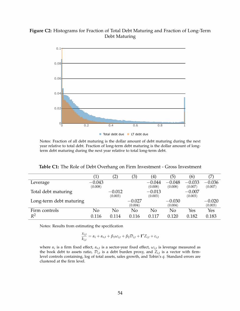
Figure C2: Histograms for Fraction of Total Debt Maturing and Fraction of Long-TermDebt Maturing

0 0.2 0.4 0.6 0.8 10

0.02

0.04

0.06

0.08

0.1

Total debt due LT debt due

Notes: Fraction of all debt maturing is the dollar amount of debt maturing during the nextyear relative to total debt. Fraction of long-term debt maturing is the dollar amount of long-term debt maturing during the next year relative to total long-term debt.

Table C1: The Role of Debt Overhang on Firm Investment - Gross Investment

(1) (2) (3) (4) (5) (6) (7)Leverage −0.043

(0.008)−0.044(0.008)

−0.048(0.008)

−0.033(0.007)

−0.036(0.007)

Total debt maturing −0.012(0.003)

−0.013(0.003)

−0.007(0.003)

Long-term debt maturing −0.027(0.004)

−0.030(0.004)

−0.020(0.003)

Firm controls No No No No No Yes YesR2 0.116 0.114 0.116 0.117 0.120 0.182 0.183

Notes: Results from estimating the specification

xi,t

ki,t= αi + αs,t + β1ωi,t + β2Di,t + Γ′Zi,t + εi,t

where αi is a firm fixed effect, αs,t is a sector-year fixed effect, ωi,t is leverage measured asthe book debt to assets ratio, Di,t is a debt burden proxy, and Zi,t is a vector with firm-level controls containing, log of total assets, sales growth, and Tobin’s q. Standard errors areclustered at the firm level.

54

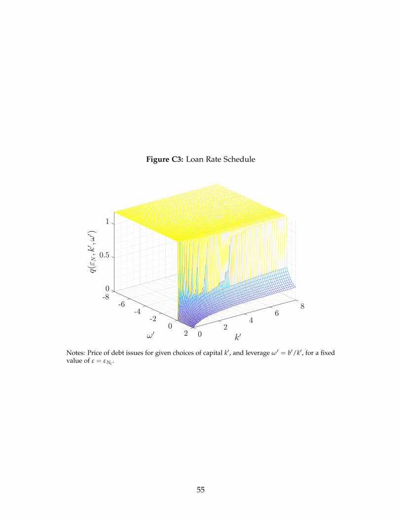
Figure C3: Loan Rate Schedule

Notes: Price of debt issues for given choices of capital k′, and leverage ω′ = b′/k′, for a fixedvalue of ε = εNε .

55

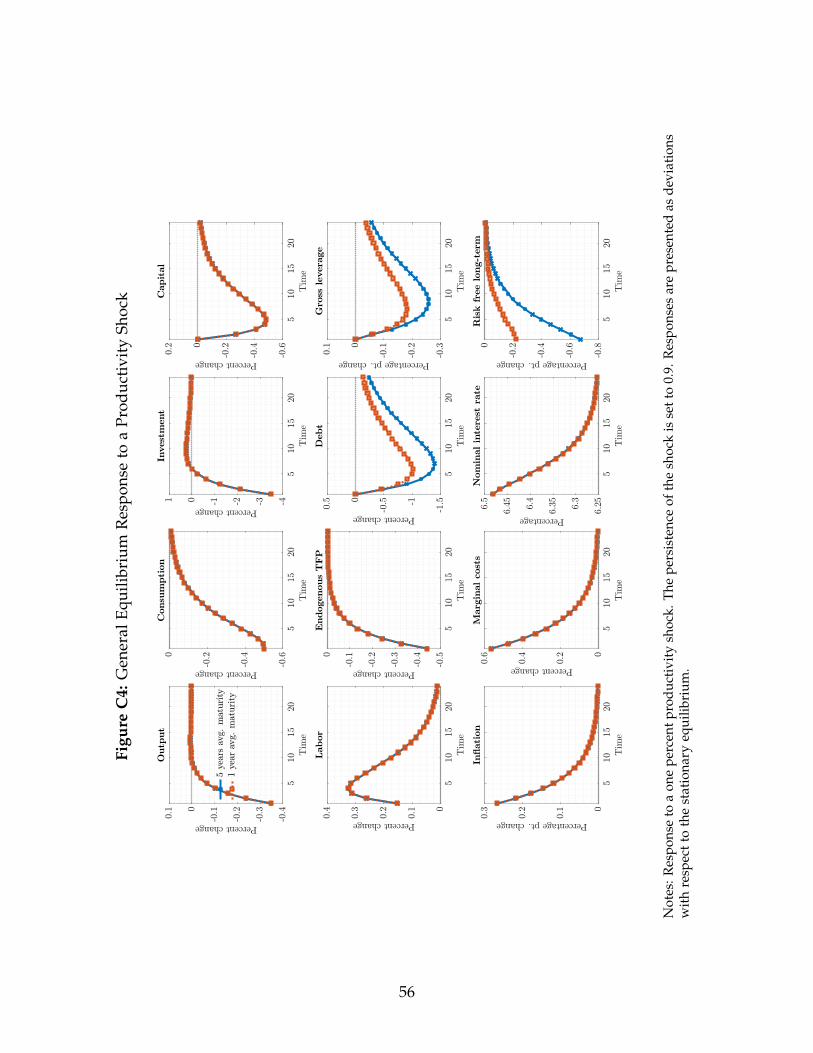
Figu

reC

4:G

ener

alEq

uilib

rium

Res

pons

eto

aPr

oduc

tivi

tySh

ock

510

1520

Tim

e

-0.4

-0.3

-0.2

-0.10

0.1

Percentchange

Outp

ut

5ye

arsav

g.m

aturity

1ye

arav

g.m

aturity

510

1520

Tim

e

-0.6

-0.4

-0.20

Percentchange

Consu

mpti

on

510

1520

Tim

e

-4-3-2-101

Percentchange

Invest

ment

510

1520

Tim

e

-0.6

-0.4

-0.20

0.2

Percentchange

Capit

al

510

1520

Tim

e

0

0.1

0.2

0.3

0.4

Percentchange

Labor

510

1520

Tim

e

-0.5

-0.4

-0.3

-0.2

-0.10

Percentchange

Endogenous

TF

P

510

1520

Tim

e

-1.5-1

-0.50

0.5

Percentchange

Debt

510

1520

Tim

e

-0.3

-0.2

-0.10

0.1

Percentagept.change

Gro

ssle

vera

ge

510

1520

Tim

e

0

0.1

0.2

0.3

Percentagept.change

In.ati

on

510

1520

Tim

e

0

0.2

0.4

0.6

Percentchange

Marg

inalcost

s

510

1520

Tim

e

6.256.3

6.356.4

6.456.5

Percentage

Nom

inalin

tere

stra

te

510

1520

Tim

e

-0.8

-0.6

-0.4

-0.20

Percentagept.change

Ris

kfr

ee

long-t

erm

Not

es:R

espo

nse

toa

one

perc

entp

rodu

ctiv

ity

shoc

k.Th

epe

rsis

tenc

eof

the

shoc

kis

sett

o0.

9.R

espo

nses

are

pres

ente

das

devi

atio

nsw

ith

resp

ect

toth

est

atio

nary

equi

libri

um.

56

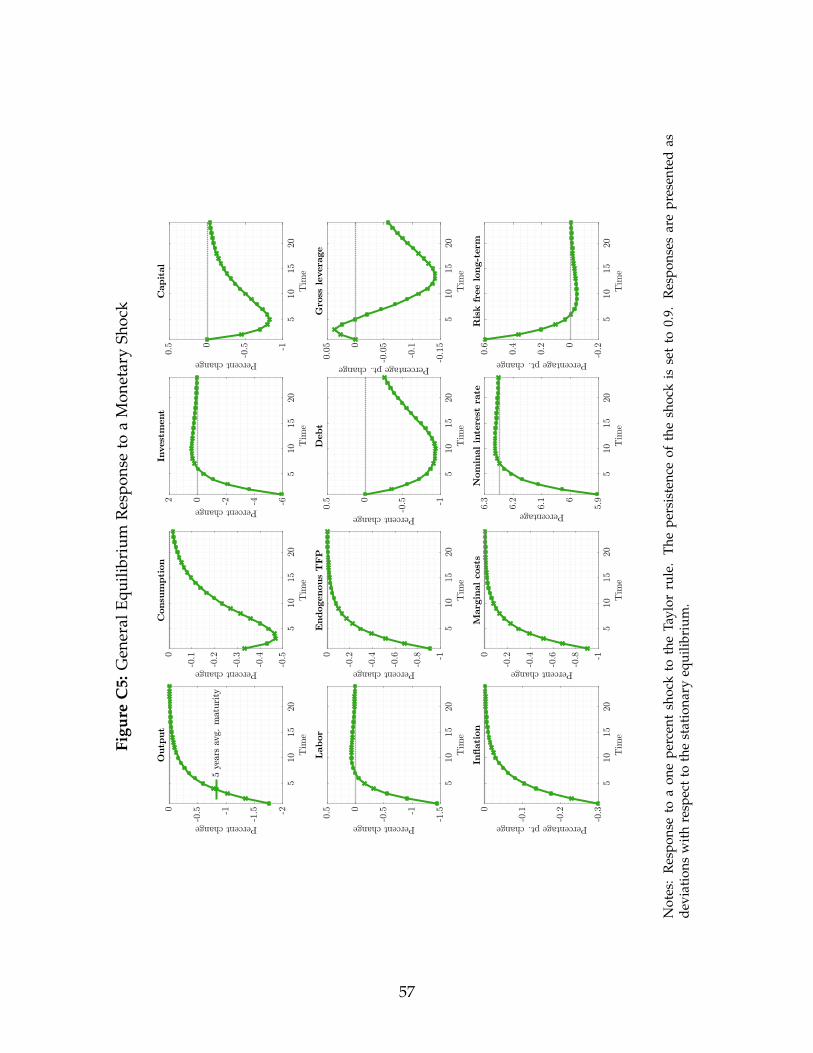
Figu

reC

5:G

ener

alEq

uilib

rium

Res

pons

eto

aM

onet

ary

Shoc

k

510

1520

Tim

e

-2

-1.5-1

-0.50

Percentchange

Outp

ut

5ye

arsav

g.m

aturity

510

1520

Tim

e

-0.5

-0.4

-0.3

-0.2

-0.10

Percentchange

Consu

mpti

on

510

1520

Tim

e

-6-4-202

Percentchange

Invest

ment

510

1520

Tim

e

-1

-0.50

0.5

Percentchange

Capit

al

510

1520

Tim

e

-1.5-1

-0.50

0.5

Percentchange

Labor

510

1520

Tim

e

-1

-0.8

-0.6

-0.4

-0.20

Percentchange

Endogenous

TF

P

510

1520

Tim

e

-1

-0.50

0.5

Percentchange

Debt

510

1520

Tim

e

-0.1

5

-0.1

-0.0

50

0.05

Percentagept.change

Gro

ssle

vera

ge

510

1520

Tim

e

-0.3

-0.2

-0.10

Percentagept.change

In.ati

on

510

1520

Tim

e

-1

-0.8

-0.6

-0.4

-0.20

Percentchange

Marg

inalcost

s

510

1520

Tim

e

5.96

6.1

6.2

6.3

Percentage

Nom

inalin

tere

stra

te

510

1520

Tim

e

-0.20

0.2

0.4

0.6

Percentagept.change

Ris

kfr

ee

long-t

erm

Not

es:

Res

pons

eto

aon

epe

rcen

tsh

ock

toth

eTa

ylor

rule

.Th

epe

rsis

tenc

eof

the

shoc

kis

set

to0.

9.R

espo

nses

are

pres

ente

das

devi

atio

nsw

ith

resp

ect

toth

est

atio

nary

equi

libri

um.

57