Debauchery and Original Sin:

The Currency Composition of Sovereign Debt 

Preliminary

Charles Engel1  JungJae Park2  

Abstract

This paper quantitatively investigates the currency composition of sovereign debt

in the presence of two types of limited enforcement frictions arising from a

government’s monetary and debt policy: strategic currency debasement and

default on sovereign debt. Local currency debt has better state contingency than

foreign currency debt in the sense that its real value can be changed by a

government’s monetary policy, thus acting as a better consumption hedge against

income shocks. However, this higher degree of state contingency for local

currency debt provides a government with more temptation to deviate from

disciplined monetary policy, thus restricting borrowing in local currency more

than in foreign currency. The two financial frictions related to the two limited

enforcement problems combine to generate an endogenous debt frontier for local

and foreign currency debts. Our model predicts that a less disciplined country in

terms of monetary policy borrows mainly in foreign currency, as the country faces

a much tighter borrowing limit for local currency debt than for the foreign

currency debt. Our model accounts for the surge in local currency borrowings by

emerging economies in the recent decade and “Mystery of Original Sin” by

Eichengreen, Haussman, Panizza (2002). (JEL: E32, E44, F34)

1 University of Wisconsin-Madison. Email: cengel@ssc.wisc.edu

2 National University of Singapore. Email: ecspj@nus.edu.sg

1

1 Introduction

“Original Sin” in the international finance literature refers to a situation in which most emerging

economies are not able to borrow abroad in their own currency. This concept, first introduced by

Eichengreen and Hausmann (1999), is still a prevailing phenomenon for a number of emerging economies,

even though the recent studies by (Du & Schreger, 2013), (Du, Pflueger, & Schreger, 2015), find that the

ability of emerging markets to borrow abroad in their own currency has been much improved in the last

decade. They find that the cross-country mean of the share of external government debt in local currency

has increased to around 60% for a sample of 14 developing countries3.

In this paper, we study the currency composition of sovereign debt in the presence of two types of

limited enforcement frictions arising from a government’s monetary and debt policy: strategic currency

debasement and default on sovereign debt. We build a dynamic general equilibrium model of a small open

economy to quantitatively investigate the implications of these two different enforcement frictions for a

government’s debt portfolio choice. In particular, we focus on how these two frictions combine to constrain

borrowing limits for local and foreign currency debt.

The temptation to debase or “debauch” the currency leads markets to restrict lending to local-

currency debt for some sovereign borrowers. This temptation has been understood by economists for many

years, though the literature lacks a full model of the dynamic contracting problem in a setting of debasement

and default. Indeed, (Keynes, 1919) asserted that “Lenin is said to have declared that the best way to destroy

the capitalist system is to debauch the currency." Keynes made this point in the context of the debate over

debt forgiveness after the First World War – countries could effectively renege on debt by debauching the

currency. (See (White & Schule, 2009) for a discussion of the context of Keynes’s famous statement.)

Our setting is a standard small open economy model with stochastic endowment shocks, extended

to allow a benevolent sovereign government to borrow in both local and foreign currency. Due to lack of

enforcement of a government’s monetary and debt policy, the government has the option to breach debt

contracts by: (1) debasing its currency to inflate away local currency debt, and (2) defaulting on both local

and foreign currency debts. Strategic debasement is punished by an “Original Sin” regime in which the

country is restricted to borrow only in foreign currency, and default is punished by permanent autarky. Risk

3 The countries in the sample are Brazil, Colombia, Hungary, Indonesia, Israel, South Korea, Malaysia, Mexico, Peru, Poland, Russia, South

Africa, Thailand and Turkey.

2

neutral foreign investors in international financial markets are willing to lend to the sovereign government

any amount, whether in local or foreign currency, as long as they are guaranteed an expected return of the

gross risk-free rate R* prevailing in the international financial markets. Since the real value of repayment

for local currency debt can change depending on the inflation rate (currency depreciation rate), the foreign

investors who lend in local currency offer a contract which specifies an inflation rate at each state of the

world. We consider an optimal self-enforcing contract which maximizes utility of the representative

household in the small open economy and which prevents the government from breaching the contract (i.e.,

satisfying the enforcement constraints).

Our model predicts that the optimal contract for local currency debt allows the government to inflate

away a certain fraction of local currency debt in times of bad income shocks but asks for currency

appreciation in times of good shocks as a compensation for the bad times. Hence, local currency debt in

our model smooths consumption of the economy better than foreign currency debt, acting like a state-

contingent asset. However, due to the limited enforcement constraint arising from a government’s

temptation to inflate away local currency debt, the borrowing limit for local currency is endogenously

constrained, thus restricting the degree of consumption smoothing function of local currency debt. On the

other hand, the enforcement constraint arising from the option to fully default on its debt mainly determines

the endogenous borrowing limit for foreign currency debt. With the interaction of two enforcement frictions,

our model generates a debt frontier for local and foreign currency debt, inside of which the equilibrium is

supported without violating the enforcement constraints.

Quantitative results show that the country with more disciplined monetary policy can borrow more

in both foreign and local currency, and that the country borrows mainly in local currency as it provides a

better consumption hedge. The country with less disciplined monetary policy wants to borrow more in local

currency, but is restricted to borrow mainly in foreign currency due to the enforcement constraints. Thus,

our model can account for both “Original Sin” phenomenon for the emerging economies with less

disciplined monetary policy and a recent surge in local currency borrowing by those with more disciplined

monetary policy.

The term “original sin” has been applied in the literature to countries that are unable to borrow in

their own currency, because empirically there seems to be very little link between the share of external debt

denominated in local currency and variables such as the volatility of inflation or the size of the country’s

total external liabilities that perhaps should determine how much the country can borrow in local currency.

We make the point that the relationship between these endogenous variables and the currency composition

of debt on the other hand is not straightforward. When there is lack of commitment to repay, there is a

tension between the wishes of the borrowers – who, for example, may wish to have high levels of local-

currency debt as a channel for smoothing consumption – and lenders who may be reluctant to lend a

3

portfolio heavily weighted toward local-currency debt to those borrowers that most desire such a portfolio.

For example, as the overall external debt of a country increases, the borrower may prefer a portfolio more

weighted toward local-currency debt, because the borrower can use inflation to make debt repayment more

state-contingent. But the lender may be less likely to offer a portfolio with a large amount of local-currency

debt in such a scenario because the temptation to deviate from the terms of the debt contract may be too

high. The currency composition of debt and variables such as the volatility of inflation or the total debt/GDP

ratio are all endogenous. They depend on parameters such as the patience and degree of risk aversion of

borrowers, the cost of default and the borrower’s cost of inflation. The model shows that there is no simple

monotonic relationship among these variables, so it is perhaps not surprising that empirically there is no

clear-cut link between the currency composition of the external portfolio and endogenous macroeconomic

variables.

1.1. Related Literature

Our work builds on the intuition from the classical argument which attributes the predominance of

foreign currency debt in international financial markets to a lack of monetary credibility. A government’s

strategic debasement to inflate away the real value of debt can pose a significant obstacle to issuing local

currency debt ( (Calvo, 1978) (Bohn, 1990) (Kydland & Prescott, 1977)). (Jeanne, 2003) presents models

in which, in the face of unpredictable monetary policy, private firms choose to borrow in foreign currency

so as to minimize their probability of default.

In contemporaneous work, Ottonello and Perez (2016) study the currency composition of sovereign

debt in the dynamic general equilibrium model of a small open economy with a government with limited

commitment to monetary and debt policy. Du et al (2014) also study the currency composition of sovereign

debt and finds that a country with higher monetary credibility borrows more in local currency. They present

a simple two period New-Keynesian model to show how credibility of monetary policy affects the currency

composition of sovereign debt. Our work is closely related to their work, but is different in that our model

builds on the literature of the optimal contract arrangements between lenders and borrowers, and

investigates how the optimal debt contract denominated in two currencies is constrained due to the two

types of commitment problems. Our model features a government’s endogenous default and debasement

decisions, which their work takes as exogenous.

We find that the interaction of the two types of a government’s strategic decisions can have

significant effects on the currency composition of sovereign debt. Our work thus contributes to a literature

which studies the optimal contract in the presence of commitment problems such as Atkeson (1991), Kehoe

and Levine (1991), Alvarez and Jermann (2000), and Bai and Zhang (2010). These studies show that

4

constrained borrowing limits arising from the limited enforcement problems can cause significant

distortions to allocations of an economy.

1.2 “Mystery of Original Sin” Revisited

Eichengreen, Hausmann, and Panizza (2002), and Haussman and Panizza (2003) find weak

empirical support for the idea that the level of development, institutional quality, or monetary credibility is

correlated with Original Sin. These studies find that only the absolute size of the economy proxied by its

GDP is robustly correlated with Original Sin. They call their finding the mystery of original sin and claim

that the original sin problem of emerging market economies is exogenous to a country’s economic

fundamentals; it is rather related to the structure of international financial system.

In this subsection, we replicate the findings of Eichengreen, Hausmann, and Panizza (2002) on an

updated data set. They run a Tobit regression in which the dependent variable is , defined as

1

, which measures the degree of Original Sin for country i. he

main explanatory variables are the GDP per capita as a proxy for the level of development of country i;

average inflation as a proxy for monetary credibility; GDP for the size of a country; and a country group

dummy variable that indicates whether country i belongs to the financial center or Europe or not. Both

and ′ are period averages of country i. They find that after controlling for country grouping, only

country size proxied by GDP is robustly correlated with a country’s ability to borrow in local currency,

refuting hypotheses that the emerging economies’ weak financial system or lack of monetary credibility

account for the Original Sin phenomenon.

We re-examine the Eichengreen, Haussman, and Panizza (2002)’s finding with updated data from

Arslanalp and Tsuda (2014), which provides a data set for external sovereign debt denominated in local

currency for 23 emerging economies4 from 2004Q1 to 2015Q4. We use the share of external local currency

debt in the total external debt as a dependent variable (LC Share) but use the same explanatory variables5

(GDP per capita, average inflation, GDP, and a dummy for European countries) as in Eichengreen,

Haussman, and Panizza (2002).

4 The countries in the sample are Argentina, Brazil, Bulgaria, Chile, China, Colombia, Egypt, Hungary, India, Indonesia, Latvia, Lithuania, Malaysia, Mexico, Peru, Philippines, Poland, Romania, Russia, South Africa, Thailand, Turkey, Ukraine. 5 The data source for these variables is World bank.

5

Table 1: LC Share and GDP LC Share

Log_GDP_PC -.098 (-1.18) -.039 (-0.45) -.043 (-0.54) Log_GDP .081 (2.02)* Europe -.179 (-1.59) -.118 (-1.09) Constant 1.25 (1.70) .801 (1.07) -1.35 (-1.07)

Absolute value of t statistics in parentheses. * Significant at 10% Eichengreen, Haussman, and Panizza (2002) use GDP per capita as a proxy for the level of

development of a country as the quality of institutions is considered to be highly correlated with GDP per

capita. They find that GDP per capita alone is highly positively correlated with the degree of Original Sin,

but after controlling for country grouping and country size, the estimated coefficient is not statistically

significant even at the 5 percent level. Table 1 reports our regression on the updated data. It is a double

censored (from 0 to 1) Tobit regression with explanatory variables of GDP per capita (measured in logs and

denoted by Log_GDP_PC in the table), GDP, and a dummy for European countries. Consistent with

Eichengreen, Haussman, and Panizza (2002), only the size of a country proxied by GDP is statistically

significant.

Table2: LC Share and Inflation

LC Share

Average Inflation -.014 (-0.78) -.008 (-0.50)

Std Inflation -.051(-1.41) -.028 (-0.74)

Max Inflation -.009 (-1.53) -.006 (-0.97)

Europe -.191(-1.85)* -.167 (-1.51) -.164 (-1.53)

Constant .465 (4.07) .509(4.66)*** .513 (4.94)*** .521 (5.25)*** .490*** (5.77) .517*** (6.25)

Absolute value of t statistics in parentheses. * Significant at 10% ** Significant at 5% *** Significant at 1%

Eichengreen, Haussman, and Panizza (2002) also investigates the cross-country correlation

between Original Sin and monetary credibility by regressing on inflation-related variables. In our

regression, we use three different proxies of monetary credibility: the average of inflation, the standard

deviation of inflation, and the maximum inflation rate for the sample period (2004-2015). Table 2 reports

the result. Even though coefficients on all three different proxies for monetary credibility are negative, all

of them are statistically insignificant, thus consistent with their findings that the inflation does not explain

6

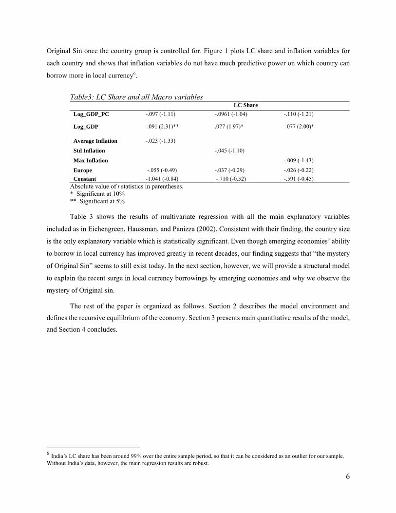
Original Sin once the country group is controlled for. Figure 1 plots LC share and inflation variables for

each country and shows that inflation variables do not have much predictive power on which country can

borrow more in local currency6.

Table3: LC Share and all Macro variables

LC Share

Log_GDP_PC -.097 (-1.11) -.0961 (-1.04) -.110 (-1.21)

Log_GDP

.091 (2.31)** .077 (1.97)* .077 (2.00)*

Average Inflation -.023 (-1.33)

Std Inflation -.045 (-1.10)

Max Inflation -.009 (-1.43)

Europe -.055 (-0.49) -.037 (-0.29) -.026 (-0.22)

Constant -1.041 (-0.84) -.710 (-0.52) -.591 (-0.45) Absolute value of t statistics in parentheses. * Significant at 10% ** Significant at 5%

Table 3 shows the results of multivariate regression with all the main explanatory variables

included as in Eichengreen, Haussman, and Panizza (2002). Consistent with their finding, the country size

is the only explanatory variable which is statistically significant. Even though emerging economies’ ability

to borrow in local currency has improved greatly in recent decades, our finding suggests that “the mystery

of Original Sin” seems to still exist today. In the next section, however, we will provide a structural model

to explain the recent surge in local currency borrowings by emerging economies and why we observe the

mystery of Original sin.

The rest of the paper is organized as follows. Section 2 describes the model environment and

defines the recursive equilibrium of the economy. Section 3 presents main quantitative results of the model,

and Section 4 concludes.

6 India’s LC share has been around 99% over the entire sample period, so that it can be considered as an outlier for our sample. Without India’s data, however, the main regression results are robust.

7

Figure 1: LC Share and Inflation

8

2. The Model Economy

We consider a standard small open economy model, extended to allow a government to borrow in

both local and foreign currency from foreign lenders in international financial markets. The representative

household receives stochastic endowment shocks every period and has preferences given by

00

[ ( ) ( )]tt t

t

E u c C

(1.1)

, where denotes the time discount factor, tc consumption, t a gross inflation rate at period t (i.e.,

(1

PtPt

), and a target inflation rate of the country. The period utility function (.)u is strictly increasing

and strictly concave, and satisfies the standard Inada conditions. Following Barro and Gordon (1983), we

introduce the cost of inflation in the form of utility loss ( )tC , which is assumed to be symmetric

around the target inflation rate ; any deviation in inflation rates from the target inflation rate incurs utility

loss. The sovereign government is benevolent and makes borrowing, default, and debasement decisions so

as to maximize social welfare of this economy.

There is one tradable consumption good, denoted by ty , in this economy. The income shock ty has

a compact support and follows a Markov process with a transition function 1Pr |t ty y . The history of

the income shock is denoted by ts . Let tP and *tP be the price of the consumption good in Home (i.e., the

small open economy) and Foreign country, respectively. We assume that the law of one price holds and the

foreign price *tP is normalized to be one, so that *

t t t tP P S S . Then the budget constraint for the

economy, conditional that the sovereign government is rolling over its debt by following the terms of

contract, is given by

* 11 1

locfor loc for t t

t t t t tt

i bc b b y R b

(1.2)

, where fortb is foreign currency debt, loc

tb local currency debt, 1ti an interest rate on local currency

debt, *R a constant gross risk-free rate prevailing in the international financial market. That is, when the

government does not breach the contract, it solves a portfolio problem between local and foreign currency

9

debt to maximize social welfare of the economy. fortb and loc

tb are non-contingent bonds in nominal terms,

but depending on the inflation rate πt, the real value of the local currency debt / tloctb can be state-

contingent.

The government can breach the debt contract in the following two ways: First, the government can

fully default on its debt denominated in both local and foreign currency simultaneously7. Second, the

government can debase its currency more than required in the contract for the local currency debt, the terms

of which will be specified in detail later. Thus our model features two types of enforcement (commitment)

frictions arising from a government’s monetary and debt policy: strategic default and debasement. This is

a novel feature of our model and we quantitatively study how these two frictions affect the currency

composition of sovereign debt.

When the government fully defaults on its debts, the economy enters permanent autarky during

which it loses access to international financial markets and suffers from a drop in income. When the

government breaches the contract by debasing its currency, the country is restricted to borrow only in

foreign currency, thus entering the “Original Sin” regime. When the government in this regime defaults

on its foreign currency debt, the economy also enters permanent autarky. Figure 2 summarizes the two

different types of breaches of the debt contract and their consequences.

7 Selective default on a certain type of debt is not allowed in our model, consistent with practices in sovereign debt markets. See Broner et al.

(2010) for theoretical study on this problem.

10

Local Currency Debt Contract

Foreign lenders in the international financial markets are risk-neutral and have deep pockets. They

are willing to lend to the sovereign government any amount, whether in local or foreign currency, as long

as they are guaranteed an expected return of the gross risk-free rate R* prevailing in the international

financial markets. Even if the local currency debt is non-contingent in nominal terms with a gross interest

rate 1ti , depending on the government’s choice on the inflation rate 1t (or equivalently depreciation

rate), the real value of repayment 11

1

loctt

t

i b

can differ. We consider the following recursive contract for the

local currency debt, which consists of two components: a nominal gross interest rate 1ti and state

contingent inflation rates in the next period 1t .

Figure 2: Two Types of Breaches of Contract

11

1 1 1( , , )for loc

t t t tb b yi (1.3)

1 1 1 1( , , , )for loc

t t t t tb b y y (1.4)

When the sovereign government borrows 1

fortb and 1

loctb in foreign and local currency in period t, the

contract charges a nominal gross interest rate 1ti on the local currency debt 1loctb . Moreover, the contract

asks for a certain inflation (depreciation) rate depending on the realization of 1ty in period t + 1.

Since the foreign investors who lend in local currency must be guaranteed an expected return of a

gross risk-free rate R* for the local currency debt, we have the following zero-profit condition on the

contract:

1

* 11

1 1 1 1

( | )( , , , )

t

tt t for loc

y t t t t t

R Pr y yb b y

i

y

(1.5)

Note that there is ty as well as 1ty in because of the persistent income shock process

1Pr |t ty y in eq (1.5).

On the other hand, the foreign lenders charge the gross risk-free rate R* on the foreign currency debt

as typical of a standard small open economy model featuring a non-contingent debt. From now on, ts

denotes the vector of state variables at period t, which consists of ( 1, ,,for loct t t tb b y y ).

Value of Debasement

Due to the limited commitment (enforcement) of monetary policy, the sovereign government can

debase its currency at any time by choosing a higher inflation rate than ( )t ts in the contract to inflate

away a certain fraction of local currency debt. When the government breaches the contract by debasing its

currency, the country is restricted to borrowing only in foreign currency thereafter as a punishment. That is,

12

the country enters the regime of “Original Sin” or foreign currency borrowing. Note that the foreign

investors who lend in foreign currency do not

incur any losses even when the government inflates away the local currency debt; they continue to lend to

the government in foreign currency after the debasement.

The value of debasement is given by

1

1 1 1( ),( , , , ) max [ ( ) ( )] ( , )for

t t t t

debase for loc for fort t t t t t t t ts b

V b b y y u c C E V b y

(1.6)

subject to the budget constraint:

*1

locfor for t t

t t t tt

i bc b y R b

forV denotes the value of borrowing in foreign currency after the debasement.

Value of Foreign Currency Borrowing (Original Sin Regime)

The value of foreign currency borrowing is given by

11 1( , ) max ( ) ( , )for

t

for for for fort t t t t tb

V b y u c E V b y

(1.7)

subject to the following constraints:

for

1for

t t t tc b y Rb

1 1 1 1( , ) ( )for for def

t t t tV b y V y for all y (1.8)

13

Equation (1.8) is the enforcement constraint related to the government’s default decision and

requires that the continuation value of foreign currency borrowing be equal to or higher than the value of

default in any possible future contingencies. Note that this enforcement constraint determines an

endogenous debt limit for the foreign currency borrowing that can be supported in equilibrium for the

Original Sin regime. 1( )deftV y denotes the value of default when the government chooses to default on

its debt, whether in local or (and ) foreign currency.

Value of Default

Upon default, the economy enters permanent autarky during which the economy loses access to the

international financial market, and the economy suffers a drop in income. The value of default is given by

1( ) ( ) ( )def deft t t tV y u c E V y (1.9)

t tc h y (1.10)

,where t th y y . th y represents a decrease in income associated with default, which is consistent

with empirical findings in the sovereign debt literature.

Original Problem under the Optimal Contract

The contract is optimal in the sense that it maximizes utility of the representative household in the small

open economy. Moreover, the contract is self-enforcing in the sense that the government under this

contract does not have any incentive to breach the contract. The original problem under the optimal self-

enforcing contract is given by:

1 1 010{ , , , }

0

max [ ( ( )) ( ( ) )]for loct t t tt

t t tt tc b b

t

E u c s C s

(1.11)

subject to (1) the budget constraint, (2) the enforcement constraint, (3) the expected zero profit

condition for the lenders.

14

* 11 1( ) ( ) ( ) ( ) ( ) ( )

( )

( )tt for t loc t t for t loc t t

t t t t t t tt

ic s b s b s y s R b s b s

s

s

(1.12)

1[ ( ) ( )] max{ ( ), ( , , , )}s t for loct s s def t debase

stt t t t

t

E u c C V y V b b y y for any y

(1.13)

1

* 11

1 1 1 1

( | )( , , , )

t

tt t for loc

y t t t t t

R Pr y yb b y

i

y

(1.14)

Then, an equilibrium in this model is a sequence of inflation rates and interest rates on local

currency debt ts and ( )tti s in the contract and allocations { , , }t for t loc t

t tc s b s b s such that the

contract and the allocations solves the maximization problem subject to the budget constraint (equation

(1.12)), the enforcement constraint (equation (1.13)), and the lender’s expected return condition (equation

(1.14)).

Note that the enforcement constraint eq (1.13) has two value functions on the right hand side: the values

of debasement and default. These enforcement constraints come from two different types of limited

commitment problems regarding the government’s monetary and debt policy. These two enforcement

constraints combine to generate an endogenous debt frontier for local and foreign currency debt, thus

determining the currency composition of sovereign debt.

Recursive Formulation of the Original Problem

Since the enforcement constraint equation (1.13) has expected values of future variables, we cannot

use the standard recursive Bellman equation, as pointed out first by the classical paper by Kyland and

Prescott (1977). This is a common problem shared with the economic models dealing with time-inconsistent

government policy. However, our original problem can be recast recursively following Atkeson (1991),

which uses the solution techniques of Abreu et al (1990) and is extended by Bai and Zhang (2010).

Before the income shock is realized at period t, the optimal contract chooses a nominal interest rate

ti and an inflation rate πt (i.e., currency depreciation rate) for each state for the period t that maximizes

the expected sum of value functions Vcs.

15

1 ( ) 1 1( , , ) max ( | ) ( , , , ; ( ))t

t

for loc c for loct t t y t t t t t t t

y

W b b y Pr y y V b b y y s (1.15)

subject to the lender’s expected zero profit condition:

1

*1

1

( | )( , , , )

t

tt t for loc

y t t t t t

R Pr y yb y

i

b y

After the income shock is realized at period t, taking ts as given, the government solves the

following value function:

111 1 1,

( , , , ; ( )) max [ ( ) ( )] ( , , )for loctt

C for loc for loct t t t t t t t t tb b

V b b y y s u c C W b b y

(1.16)

*1 1 ( )

locfor loc for t t

t t t t tt

i bc b b y R b

s (1.17)

'

1 1 1 1 1 1 1 1 1( , , , ; ( )) max{ ( , , , ), ( )}C for loc debase for loc def st t t t t t t t t t tV b b y y s V b b y y V y for all y

(1.18)

Following Atkeson (1991) and Bai and Zhang (2010), we solve the above problem iteratively starting

with sufficiently high initial values 0W and 0V , where the subscript denotes the number of iterations. At

each iteration, the domain 0D of 0W and 0V is updated such that it solves the maximization problems of

equations ((1.15), (1.16)) subject to the budget and the enforcement constraints eq ((1.17), (1.18)). The

sequences of {Wn} ,{Vn}, and {Dn} are decreasing, finally converging to W,V, and D, respectively. Then,

we have combinations of ( locb ,  forb ) in D that satisfy the budget and the enforcement constraint.

For the interior solutions of t and ti , we have the following first order conditions.

2 2[ ( )] : '( , ) '( )) ) '( , ) '( ))( ( )( (i i i loc i i loct t t t t t t t t t t t

j jt

j jss u s y i b C u s y i b C for is js s

(1.19)

1[ ] : Pr( | ) '( )( ) ) 0(it

i i it t ttt

yti y y C s s (1.20)

, where i denotes an income shock iy , and i jy y for i j .

16

At optimum, the first term on the left hand side is the benefit of a marginal increase in an inflation

rate: an increase in inflation rates leads to a decrease in the real value of local currency debt, thus increasing

consumption at the state of ( , )i it ts y . Note that the first term on the left hand side has loc

tb ; the more local

currency debt the economy holds at period t, the higher the marginal benefit of an increase in inflation rates

is. The second term on the left hand side is the marginal cost of the increase in inflation rates. If there is an

increase in inflation rates (i.e., depreciation) at the state ( , )i it ts y , the zero profit condition for the foreign

lenders (eq ((1.21) ) requires a decrease in inflation rates (i.e., appreciation) at other states ( , )jt t

js y to

compensate for the loss incurred to the lenders at state ( , )i it ts y . The right hand side is the marginal cost

associated with the appreciation of the currency. That is, the optimal contract equates the marginal benefit

and cost across states.

The first order condition with respect to ti shows that at optimum, the nominal interest rate ti on

the local currency debt is chosen to minimize the expected sum of costs of inflation across states. Note that

with a symmetric cost of inflation around the target inflation rate , the marginal cost at t is negative.

The following proposition and corollary characterize the state-contingent nature of local currency

debt in our model.

Proposition 1: Suppose that there is no enforcement constraint (eq(1.18)) and that there is no cost

of inflation (i.e., tC = 0 for all t ). Then the optimal contract for the interior solutions is such

that

( , ) ( , ) .i i j j

t t t tc s y c s y for any i j (1.22)

Proof: See the Appendix

This proposition shows that local currency debt has characteristics similar to the Arrow-securities in the

complete markets model. Without any financial frictions and cost of inflation, the local currency debt

smoothes consumption of the representative household across states.

17

Corollary 1: Suppose that i jt ty y . Then, under the same conditions as the proposition 1, t on

the optimal contract is such that

( , )) ( , )i i j j

t t t ts y s y (1.23)

The corollary shows that without any frictions, the optimal contract for the local currency debt

allows the government to depreciate its currency in times of bad income shocks but asks for currency

appreciation in times of good income shocks as a compensation to the investors for the bad times. Thus,

compared to the foreign currency debt, local currency debt under the optimal contract is a better instrument

for consumption hedging against the income shock.

Debt Frontier

Let locb be the maximum debt amount for local currency debt supported in equilibrium, which is

given by

1 1 1 1{ : (0, , , ) max{ (0, , , ), ( )} ( , )loc loc c loc debase loc def

t t t t t t tb min b V b y y V b y y V y for all y y s

(1.24)

That is, locb is the maximum borrowing limit for local currency debt without any borrowing in

foreign currency (i.e., forb = 0) that can be supported in equilibrium without violating the enforcement

constraints. Note that b denotes bond holdings, not debt.

Then the debt frontier, which is a function of bloc, is defined as the following:

1 1 1

1

( ) { : ( , , , ) max{ ( , , , ), ( )}}

0 ( , ),

for loc for c for loc debase for loc deft t t t t

loc loct t

b b min b V b b y y V b b y y V y

for b and all y yb s

(1.25)

That is, ( )for locb b is the maximum amount of borrowing in foreign currency, given that the economy

chooses to borrow bloc in local currency. Any more borrowing than ( )for locb b violates the enforcement

constraints, thus not supported in equilibrium.

18

Proposition 2: Suppose that the cost of the inflation C(π t;ξ) is differentiable and strictly increasing in t , and that ( ; )tC is strictly increasing and convex in for any t . Then

, , loc H loc L H Lforb b .

That is, a country with a higher cost of inflation has a more relaxed debt limit for local currency debt.

Proof: See the Appendix

Proposition 2 shows that the degree of monetary credibility represented by the cost of inflation

parameter determines the borrowing limit for local currency debt. This is consistent with the recent

empirical findings by Du et al (2014) which show that in the recent decades, even developing countries

with more disciplined monetary policy have managed to borrow more in local currency, which departs from

the trend of “Original Sin” in the 70’s and 80’s.

Proposition 3: Under the same conditions in the proposition 2, If then 1tt s .

Moreover, the currency composition between foreign and local currency debts is indeterminate.

When the cost of inflation is infinite, the foreign currency debt becomes the same as the local currency debt,

so the currency composition between two types of debts is indeterminate.

19

3 Quantitative Results

3.1 Parameters and Functional Forms

In this section, we solve the model numerically and simulate it to investigate quantitative

implications of the two limited commitment frictions for the currency composition of sovereign debt.

Table 4 reports the parameters used for the benchmark calibration. A period is a year. We use the

standard CRRA utility function 1 1

1

c

and set to be 2, which is standard in the literature. The time

discount factor is set to be 0.96.

The income shock takes on two values, Hy and Ly , where and . is the

mean income and the standard deviation of the income shock. The mean income is normalized

to be one, and is set to be 4%. As a benchmark case, we assume that shocks are i.i.d for the

benchmark calibration.

We use the quadratic cost of inflation given by

2( ) ( 1)C (1.26)

20

, which implies that the target inflation rate is normalized to be one.

The cost of default during autarky is in the form of a drop in income: ( ) (1 )t th y y (1.27)

As with other studies in the sovereign debt literature, we assume that the economy suffers from a

drop in income during autarky. As a benchmark value, we set to be 0.03 from Benjamin and Wright

(2009).

3.2 Model Moments

Table 5: Model Moments

. .

locb (% of GDP) 31.2% 50.1%

Average Total Debt (% of GDP) 63.65% 62.70%

Average LC Debt (% of GDP) 13.77% 34.47%

Average LC Share (%) 22.92% 58.45%

Corr (GDP, Total Debt) -0.41 -0.43

Corr (GDP, LC Share) 0.22 0.40

Corr (GDP, inflation rate) -0.85 -0.84

Std (inflation rate) 13.57% 2.287%

Table 5 compares the model moments regarding debt and inflation for the cases of low ( . and

high ( . ) cost of inflation. To get the statistics in Table 5, we simulate the model 5000 times and

the first 1000 simulated data points are removed to rule out any effects of initial conditions.

21

For the high cost of inflation ( . , the maximum local currency debt limit is 0.312,

whereas for the low cost of inflation ( . , the maximum local currency debt limit is 0.501. That

is, a high cost of inflation is associated with a more relaxed borrowing limit for the local currency debt. The

total debt-the sum of local and foreign currency debts- is on average not much different between the two

cases. However, the average local currency debt and local currency share in total debt shows a significant

difference between the two cases: the economy with a high cost of inflation borrows on average more (34.47%

of its GDP) than that with a low cost of inflation (13.77% of its GDP). Moreover, the local currency debt

shares for the high and low cost inflation cases are 58.45% and 22.92, respectively. As the local currency

debt limit with a high cost of inflation is more relaxed than that with a low cost of inflation, the economy

with a high cost of inflation tends to borrow more in local currency.

For both cases, the correlation between GDP and inflation is negative at around -0.85, consistent

with the Corollary 1; the optimal contract asks for depreciation in bad income times but asks for

appreciation in good income times. However, the economy with a low cost of inflation uses monetary policy

more actively to use the local currency debt as a consumption-hedging device. The last row of the table

reports volatilities of inflation for the two cases.

22

3.3. Debt Frontiers for Different Costs of Inflation

Figure 3: Debt Frontiers with Different Costs of Inflation ( . .

Figure 3 plots two debt frontiers for two different values of cost of inflation ( .

. . The debt frontier shows the maximum debt limits for both types of debts supported in equilibrium

without violating the enforcement constraints. For the case of the high cost of inflation, the debt frontier is

a dashed black line, and for the case of the low cost of inflation, the debt frontier is a red line. The region

under the frontier is feasible combinations of local and foreign currency debts that the government can

choose without violating the enforcement constraints. Note that the region for the high cost of inflation is

strictly larger and covers that for the low cost of inflation. That is, the country with more disciplined

monetary policy is able to borrow more in both local and foreign currency debts. However, the debt frontier

for the low cost of inflation is more restricted along the dimension of local currency debt.

23

3.4. Debt Frontiers for Different Costs of Default

Figure 4: Debt Frontiers with Different Costs of Default ( . .

Figure 4 plots two debt frontiers for two different values of cost of default ( . .

with . and other benchmark parameters. For the low cost of default, the borrowing limits for

local can foreign currency debt (solid red line) are much tighter than those for the high cost of default.

24

3.5 Further Numerical Results

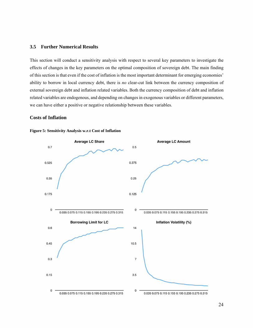
This section will conduct a sensitivity analysis with respect to several key parameters to investigate the

effects of changes in the key parameters on the optimal composition of sovereign debt. The main finding

of this section is that even if the cost of inflation is the most important determinant for emerging economies’

ability to borrow in local currency debt, there is no clear-cut link between the currency composition of

external sovereign debt and inflation related variables. Both the currency composition of debt and inflation

related variables are endogenous, and depending on changes in exogenous variables or different parameters,

we can have either a positive or negative relationship between these variables.

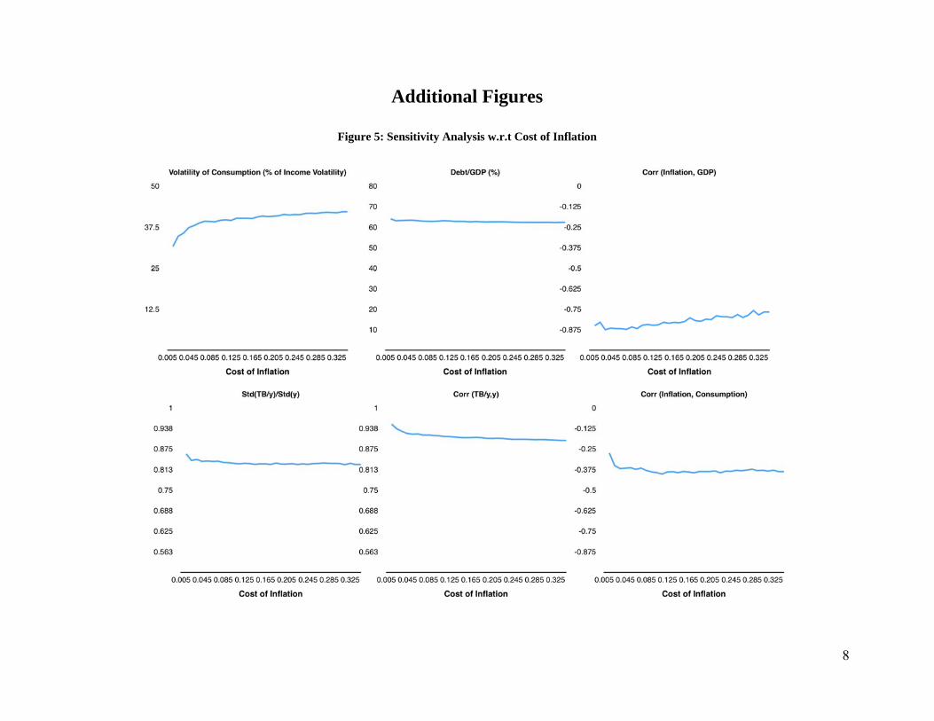
Costs of Inflation

Figure 5: Sensitivity Analysis w.r.t Cost of Inflation

25

Figure 5 plots average share of local currency debt, average local currency debt amounts, borrowing limits

for the local currency debt, and volatilities of inflation for different values of from 0.005 through 0.335.

As the cost of inflation increases, the economy can borrow more in local currency as shown in the increase

in the borrowing limit for local currency debt (the left panel in the bottom). Accordingly, the average LC

share and local currency debt amount increase. Moreover, the volatility of inflation decreases as the cost of

inflation increases.

The predictions of the model are consistent with two empirical facts regarding “Original Sin”

phenomenon: First, the emerging economies which suffered high inflation volatility during the 80s and 90s

borrowed mostly in foreign currency. Second, the emerging economies which have gotten increasingly

more disciplined in monetary policy are more likely to borrow in local currency during the last decade. That

is, our model can predict both “Original Sin” phenomenon for the emerging economies in the 80s and 90s

and a recent surge in local currency borrowings for the emerging economies with more disciplined monetary

policy.

26

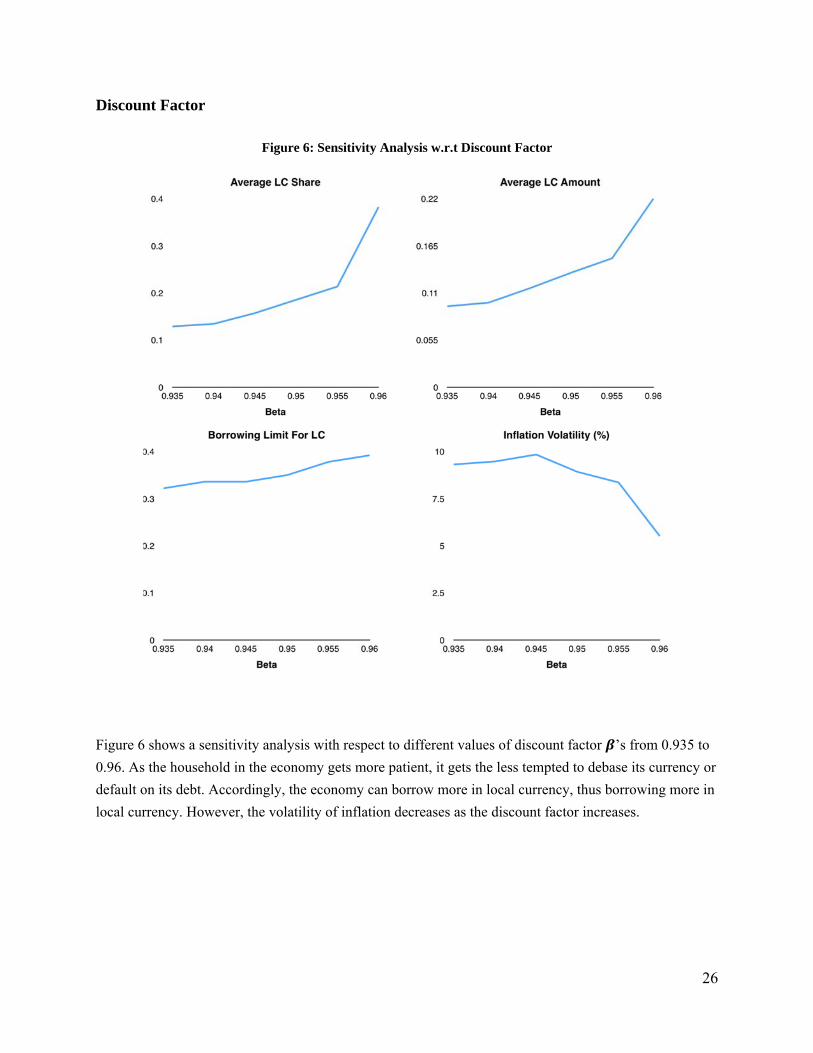
Discount Factor

Figure 6: Sensitivity Analysis w.r.t Discount Factor

Figure 6 shows a sensitivity analysis with respect to different values of discount factor ’s from 0.935 to

0.96. As the household in the economy gets more patient, it gets the less tempted to debase its currency or

default on its debt. Accordingly, the economy can borrow more in local currency, thus borrowing more in

local currency. However, the volatility of inflation decreases as the discount factor increases.

27

Risk Aversion

Figure 7: Sensitivity Analysis w.r.t Gamma

Figure 7 shows a sensitivity analysis with respect to different values of ′ . As the household gets more

risk averse, they value more on consumption smoothing, thus prefer local currency debt. Hence, the

borrowing limit for the local currency debt increases with . Even though the local currency share of debt

increases, the inflation volatility increases, which is different from the predictions for the cases of increasing

. As the household gets more risk-averse, the economy borrows more in local currency and actively

conducts monetary policy to smooth consumption, taking advantage of state-contingent nature of local

currency debt.

28

Output Cost of Default

Figure 8: Sensitivity Analysis w.r.t Output Cost of Default

Figure 8 shows a sensitivity analysis with respect to different output cost parameter of ′ . As the cost of

output for default increases, the borrowing limit for local currency increases, and the economy borrows

more in local currency. However, the average local currency share decreases with . The debt frontier gets

enlarged as the output cost of default increases; however as shown in the figure 2, compared to the local

currency debt, the borrowing limit for foreign currency debt gets more relaxed; the economy tends to

borrow more in foreign currency than in local currency, even if the absolute amount of local currency debt

increases with .

29

Persistence of Income Shock

Figure 9: Sensitivity Analysis w.r.t Persistence of Income Shock

Figure 9 shows a sensitivity analysis with respect to different degrees of persistence of the income shock

process. As the income shock gets more persistence, the value of debasement/default increases; when a

good income shock hits the economy, the good income shock is expected to persist for a long period of

time, thus increasing the value of breaching the contract. This is reflected in the decrease in the borrowing

limit for the local currency debt with an increase in the degree of persistence. However, the average local

currency share and amount of local currency debt shows a non-monotonic shape in the degrees of

persistence.

30

Income Variance

Figure 10: Sensitivity Analysis w.r.t Income Variance

Figure 10 shows a sensitivity analysis with respect to different income variances. As the income

variance increases, the value of breaching the contract decreases; the value of debasement and default

decrease because the economy has less efficient consumption smoothing vehicle in the “Original Sin”

regime and permanent autarky. As the income variance increase, the borrowing limit for local currency debt

increases. The average local currency share and amount of local currency debt shows a U-shape in the

income variance. The inflation volatility follows the shape of the average local currency share as the income

variance increases.

31

3.6 Why Still We Have Mystery of Original Sin ?

In the section 1.2, we find that “mystery of original sin” still exists today from the regression result

that there are no meaningful economic regressors except for the absolute size of a country to account for

Original Sin of emerging economies. However, the findings in the previous sensitivity analysis show why

we have weak empirical support for the hypothesis that monetary credibility and weak institution of

emerging economies are the main cause of Original Sin.

Table 6: Correlation between LC share and Inflation Volatility

Parameters Correlation (LC share, Inflation Volatility)

Cost of Inflation negative

Discount Factor negative

Risk Aversion positive

Output Cost of Default non-monotonic

Persistence of Income Shock positive

Volatility of Income Shock positive

Table 6 summarizes the correlations between LC share and inflation volatility in simulation with

respect to changes in key parameters in our model. With respect to the change in parameters for cost of

inflation and the discount factor, the LC share and inflation volatility move in the same direction. On the

other hand, with respect to the change in parameters for the degree of risk-aversion, and persistence and

volatility of income shock, the LC share and inflation volatility move in the opposite direction. With respect

to the change in the parameter for the output cost of default, we don’t see any monotonic relationship

between the two variables.

Figure 10 shows two scatterplots of LC share and volatility of inflation and illustrates this point

more clearly. The red lines in the left panel of Figure 9 show movements in (LC share and volatility of

inflation) pairs for two different costs of inflation as the income variance increases, fixing other parameters

at the benchmark values. The pair moves toward northeast as the income variance increases. The blue

dashed line shows movements in (LC share and volatility of inflation) pairs as the cost of inflation parameter

increases, fixing other parameters at the benchmark values. The pair moves toward northwest as the cost

of inflation increases. The red line in the right panel of Figure 10 tracks movements in (LC share and

volatility of inflation) pairs as the degree of risk-aversion increases. The pair in red line moves toward

northwest as the degree of risk-aversion increases. The blue dashed line in the right panel is the same as

that in the left panel.

32

Figure 10: Scatterplots of Volatility of Inflation and LC Share

The figure 10 shows that even though emerging economies have been able to borrow more in local

currency due to more disciplined monetary policy in the last decade8, we can still have weak empirical

support for the hypothesis that lack of monetary credibility is the root cause of Original Sin.

Our model predicts that the monetary credibility associated with the cost of inflation is the most

important determinant for emerging economies’ ability to borrow in local currency debt, but both inflation

and the local currency share of external sovereign debt are endogenous variables, so that for countries with

different characteristics (e.g., different degree of patience, risk-averseness, etc.) we can observe a non-

monotonic relationship between inflation and LC share in the data as shown in the Figure 1.

8 See Ebeke and Fouejieu (IMF Working Paper 2015)

33

4 Conclusions

This paper quantitatively investigates the currency composition of sovereign debt in the presence of two

types of limited enforcement problems arising from a government’s monetary and debt policy: strategic

currency debasement and default on sovereign debt. Local currency debt has better state contingency than

foreign currency debt in the sense that its real value can be changed by a government’s monetary policy,

thus acting as a better consumption hedge against income shocks. However, this higher degree of state

contingency for local currency debt provides a government with more temptation to deviate from

disciplined monetary policy, thus restricting borrowing in local currency more than in foreign currency.

The two financial frictions related to the two limited enforcement problems combine to generate an

endogenous debt frontier for local and foreign currency debt. Our model predicts that a less disciplined

country in terms of monetary policy borrows mainly in foreign currency, as the country faces a much tighter

borrowing limit for the local currency debt than for the foreign currency debt. The prediction of our model

is consistent with the “Original Sin” phenomenon and can also account for a surge in local currency

borrowing by emerging economies in the recent decades.

34

Appendix 1 : Proof of the Propositions

Proposition 1: Suppose that there is no enforcement constraint (eq(1.18)) and that there is no cost

of inflation (i.e., tC = 0 for all t ). Assume that the optimal debt levels and inflation rates

( )tt s on the contract are interior. Then the optimal contract is such that

( ( , )) ( ( , )) .i i j j

t t t tu c s y u c s y for any i j (2.1)

Proof] The Envelope condition for Vc with respect to π(s) is given by

2( ( ))

( )

locc t ti b

V u c s for all ss

The Lagrangean for the equation (1.15) is given by

*( ) 1 1 1max ( | ) ( , , , ; ( )) { ( | ) }

( )s s

c for loc ts s t t t t t t s t

y y s

L Pr y y V b b y y y Pr y yi

Ry

The first order condition w.r.t π(si) is given by

1 1 2

1( | ) ( ) ( | ) 0

( )c

si t i si tsi

Pr y y V s Pr y yy

2 2( ) ( ) ( ) ( )i

c ci s j jV s y V s s

Combining the first order conditions and the envelope condition, we have:

( ( )) ( ( ))loc loci t t j t tu c s i b u c s i b

Since btloc ≠ 0, we have the following:

( ( , )) ( ( , ))i i j jt t t tu c s y u c s y for any i j

35

Proposition 2: Suppose that the cost of the inflation C(π t;ξ) is differentiable and strictly increasing in t , and that ( ; )tC is strictly increasing and convex in for any t . Then

, , loc H loc L H Lforb b .

Proof: The Envelope conditions for the values of debasement and contract w.r.t ξ are identical with

-Cξ(πt), where (.)C denotes a partial derivative w.r.t . However, the inflation rate for the case

of debasement debase must be higher than that of the contract, as the government does not follows

the inflation rate in the contract πt*. Thus, we have that

Vξdebase(0, bloc, yt, yt  + 1) =  − Cξ(πt

debase) <  − Cξ(πt*) = Vξ

con(0, bloc, yt, yt  + 1) for all bloc, yt, yt  + 1.

That is, an increase in ξ leads to a decrease in both value functions Vdebase and Vcon , but Vdebase

decreases more than Vcon. Recall that ,loc Lb is defined as follows:

, , ,

1 1 1 1{ : (0, , , ) max{ (0, , , ), ( )}} ( , )loc L loc con loc L debase loc L defL t t L t t t t tb min b V b y y V b y y V y for all y y

(2.2)

,where subscript L denotes the value function associated with the cost of inflation C(πt;ξL). If we

increase ξ at ξL, the difference between the right and left hand side

1,

1max{ 0, , , , }locon debase defL L t t

c LtV V b y y V y is increasing or stays the same. Since both Vcon

and Vdebase are strictly increasing in locb , there exists locb ≤ ,loc Lb that satisfies the inequality ((2.2))

for H > L .

36

Bibliography

Abreu, D., Pearce, D., & Stacchetti, E. (1990). Toward a theory of discounted repeated games with imperfect monitoring. Econometrica, 1041-1063.

Aiyagari, S. R. (1994). Uninsured idiosyncratic risk and aggregate saving. The Quarterly Journal

of Economics, 659-684. Alvarez, F., & Jermann, U. J. (2000). Efficiency, equilibrium, and asset pricing with risk of default.

Econometrica, 775-797. Arslanalp, Mr Serkan, and Mr Takahiro Tsuda. Tracking global demand for emerging market sovereign debt. No. 14-39. International Monetary Fund, 2014. Atkeson, A. (1991). International lending with moral hazard and risk of repudiation. Econometrica,

1069-1089. Bai, Y. B., & Zhang, J. (2010). Solving the Feldstein—Horioka puzzle with financial frictions.

Econometrica, 603-632. Barro, R. J., & Gordon, D. B. (1983). Rules, discretion and reputation in a model of monetary

policy. Journal of monetary economics, 101-121. Bohn, H. (1990). A positive theory of foreign currency debt. Journal of International Economics,

273-292. Broner, F., Martin, A., & Ventura, J. (2010). Sovereign risk and secondary markets. 1523-1555. Calvo, G. A. (1978). On the time consistency of optimal policy in a monetary economy.

Econometrica, 1411-1428. Du, W., & Schreger, J. (2013). Local currency sovereign risk. FRB International Finance

Discussion Paper. Du, W., Pflueger, C. E., & Schreger, J. (2015). Sovereign Debt Portfolios, Bond Risks, and the

Credibility of Monetary Policy. Working Paper. Du, W., Schreger, J., & al, e. (2014). Sovereign Risk, Currency Risk, and Corporate Balance Sheets.

Working Paper. Ebeke, Christian, and Armand Fouejieu. "Inflation Targeting and Exchange Rate Regimes in Emerging Markets." (2015). Eichengreen, B., & Hausmann, R. (1999). Exchange rates and financial fragility. NBER Working

Paper.

37

Eichengreen, B., Hausmann, R., and Panizza, U., (2002). "Original Sin: The Pain, the Mystery and the Road to Redemption", paper presented at a conference on Currency and Maturity Matchmaking: Redeeming Debt from Original Sin, Inter-American Development Bank Jeanne, O. (2003). Why do emerging economies borrow in foreign currency? IMF Economic

Review. Kehoe, T. J., & Levine, D. K. (2007). Debt-Constrained Asset Markets. The Review of Economic

Studies, 865-888. Keynes, J. M. (1919). The economic consequences of the peace. Kocherlakota, N. (1996). Implications of Efficient Risk Sharing without Commitment. The Review

of Economic Studies , 63, 595-609. Kydland, F. E., & Prescott, E. C. (1977). Rules rather than discretion: The inconsistency of optimal

plans. The journal of political Economy, 473-491. Hausmann, Ricardo, and Ugo Panizza. "On the determinants of Original Sin: an empirical investigation." Journal of international Money and Finance 22.7 (2003): 957-990. Tauchen, G. (1986). Finite state markov-chain approximations to univariate and vector

autoregressions. Economics Letters, 177-181. White, M., & Schule, K. (2009). Retrospectives: Who Said Debauch the Currency: Keynes or

Lenin? The Journal of Economic Perspectives, 213-222.

38

8

Additional Figures

Figure 5: Sensitivity Analysis w.r.t Cost of Inflation

9

Figure 6: Sensitivity Analysis w.r.t Discount Factor

10

Figure 7: Sensitivity Analysis w.r.t Risk-Averseness

11

Figure 8: Sensitivity Analysis w.r.t Output Cost of Default

12

Figure 9: Sensitivity Analysis w.r.t Persistence of Income Shock

13

Figure 10: Sensitivity Analysis w.r.t Variance of Income Shock