Dealing with hurricane surge flooding in a changing ...

ORIGINAL PAPER

Dealing with hurricane surge flooding in a changing environment:part I. Risk assessment considering storm climatology change,sea level rise, and coastal development

Ning Lin1 • Eric Shullman1

Published online: 21 February 2017

� The Author(s) 2017. This article is published with open access at Springerlink.com

Abstract Coastal flood risk will likely increase in the

future due to urban development, sea-level rise, and

potential change of storm surge climatology, but the latter

has seldom been considered in flood risk analysis. We

propose an integrated dynamic risk analysis for flooding

task (iDraft) framework to assess coastal flood risk at

regional scales, considering integrated dynamic effects of

storm climatology change, sea-level rise, and coastal

development. The framework is composed of two compo-

nents: a modeling scheme to collect and combine necessary

physical information and a formal, Poisson-based theoret-

ical scheme to derive various risk measures of interest.

Time-varying risk metrics such as the return period of

various damage levels and the mean and variance of annual

damage are derived analytically. The mean of the present

value of future losses (PVL) is also obtained analytically in

three ways. Monte Carlo (MC) methods are then developed

to estimate these risk metrics and also the probability dis-

tribution of PVL. The analytical and MC methods are

theoretically and numerically consistent. A case study is

performed for New York City (NYC). It is found that the

impact of population growth and coastal development on

future flood risk is relatively small for NYC, sea-level rise

will significantly increase the damage risk, and storm cli-

matology change can also increase the risk and uncertainty.

The joint effect of all three dynamic factors is possibly a

dramatic increase of the risk over the twenty-first century

and a significant shift of the probability distribution of the

PVL towards high values. In a companion paper (Part II),

we extend the iDraft to perform probabilistic benefit-cost

analysis for various flood mitigation strategies proposed for

NYC to avert the potential impact of climate change.

Keywords Coastal flood risk � Climate change �Hurricanes � Storm surge � Sea-level rise

1 Introduction

Tropical cyclones (TCs; aka hurricanes) have induced

devastating storm surge flooding worldwide (e.g., Hurri-

canes Katrina of 2005 and Sandy of 2012 in the U.S.,

Cyclone Nargis of 2008 in Myanmar, and Typhoon Haiyan

of 2013 in Philippines). The impacts of these storms may

worsen in the coming decades because of rapid coastal

development (Curtis and Schneider 2011) coupled with

sea-level rise (Nicholls and Cazenave 2010) and possibly

increasing TC activity due to climate change (Bender et al.

2010; Knutson et al. 2010; Emanuel 2013). Major advances

in coastal flood risk management are urgently needed

(NRC 2014; Rosenzweig and Solecki 2014). Given the

inherent uncertainties in the future climate and social/

economic systems, such risk management should be

strongly informed by probabilistic risk assessment (Lin

2015).

Various methods of ‘‘catastrophe loss modeling’’ have

been developed over the past decades to assess coastal

flood risk (Grossi et al. 2005; Wood et al. 2005; Cza-

jkowski et al. 2013, among others). These approaches

combine modeling of the hazards (i.e., storm surges

induced by tropical and/or extratropical cyclones) and

information about the exposure and vulnerability to quan-

tify potential losses and risk. Most of these methods,

however, model the hazards primarily based on historical

& Ning Lin

[email protected]

1 Department of Civil and Environmental Engineering,

Princeton University, Princeton, NJ, USA

123

Stoch Environ Res Risk Assess (2017) 31:2379–2400

DOI 10.1007/s00477-016-1377-5

http://orcid.org/0000-0002-5571-1606

http://crossmark.crossref.org/dialog/?doi=10.1007/s00477-016-1377-5&domain=pdf

http://crossmark.crossref.org/dialog/?doi=10.1007/s00477-016-1377-5&domain=pdf

records with ‘‘stationary’’ assumptions and thus are not

readily applicable to estimate risk in a changing or ‘‘non-

stationary’’ climate. The effect of climate change may be

accounted for with pre-assumed factors for sensitivity

analyses (Ou-Yang and Kunreuther 2013). To obtain more

objective projection of future risk, the catastrophe loss

modeling is better coupled with state-of-the-art climate

modeling (Hall et al. 2005; Hallegatte et al. 2010). How-

ever, only a few studies have translated model-projected

climate change to social/economic impacts (Tol 2002a, b;

Mendelsohn et al. 2012), and analytical frameworks for

projecting future damage risk, especially those related to

extreme weather events, are still sparse (Bouwer 2013).

To build a comprehensive framework for projecting

future storm surge flood risk, it is necessary to consider

climate-model projected change in the relative sea level

(RSL; including the effect of land subsidence) and storm

surge climatology (i.e., surge frequency and magnitudes)

and economic/social-model projected change in the expo-

sure and vulnerability. Various studies have incorporated

RSL projections in estimating future flood hazards (Gornitz

et al. 2001; Tebaldi et al. 2012; Hunter et al. 2013; Orton

et al. 2015; Wu et al. 2016, among others) and flood

damage risk (Wu et al. 2002; Kleinosky et al. 2006;

Nicholls and Tol 2006; Hallegatte et al. 2011; Hoffman

et al. 2011; Hinkel et al. 2014, among others), where

projected change in exposure and vulnerability (Jain et al.

2005) have also often been considered. While most of these

studies have considered RSL scenarios and/or ranges

(Houston 2013), more recently, Kopp et al. (2014) devel-

oped probabilistic projections of RSL for various coastal

sites globally. Such probabilistic projections of local RSL

have been used to estimate future flood hazard probabilities

(Buchanan et al. 2015), and they can be further applied to

quantify flood damage risk (Lickley et al. 2014).

Potential change in storm surge climatology, on the

other hand, has seldom been considered in estimating

future flood hazard and damage risk. One reason is that

relatively large uncertainties still exist regarding how cli-

mate change will affect TCs (Knutson et al. 2010; Emanuel

2013). Another reason is that TCs (unlike extratropical

cyclones) cannot be well resolved in typical climate models

due to TCs’ relatively small scales (except perhaps in a

recently-developed high-resolution climate model, Mur-

akami et al. 2015). Dynamic downscaling methods can be

used to better resolve TCs in climate-model projections

(Knutson et al. 2013, 2015), but most of these methods are

computationally too expensive to be directly applied to risk

analysis. Statistical models have been developed to gen-

erate synthetic TCs that can vary with influential climate

variables such as sea surface temperature (Vickery et al.

2009; Hall and Yonekura 2013; Mudd et al. 2014; Elling-

wood and Lee 2016). The statistical-deterministic model

developed by Emanuel et al. (2006, 2008), however, is

currently the primary method that can generate large

numbers of synthetic TCs with physically correlated

characteristics (i.e., frequency, track, intensity, size) driven

by comprehensive (observed or projected) climate condi-

tions involving the environmental wind and humidity,

thermodynamic state of the atmosphere, and thermal

stratification of the ocean. This probabilistic TC model has

been integrated with hydrodynamic surge models (Wes-

terink et al. 2008; Jelesnianski et al. 1992) into a clima-

tological-hydrodynamic method (Lin et al.

2010, 2012, 2014; Lin and Emanuel 2016) to generate large

samples (*104) of synthetic storm surge events and assess

the surge hazard probabilities. This method has been

applied to investigate storm surge hazards under observed

and/or projected climate conditions for various coastal

cities, including New York City (NYC; Lin et al.

2010, 2012; Reed et al. 2015); Miami (Klima et al. 2012)

and Tampa (Lin and Emanuel 2016) in Florida; Galveston

in Texas (Lickley et al. 2014); Cairns in Australia (Lin and

Emanuel 2016); and Dubai in the Persian Gulf (Lin and

Emanuel 2016).

Such city-scale storm surge hazard estimations can be

applied to flood damage risk assessment. First, the gener-

ated synthetic surge events under observed/current climate

conditions can be conveniently translated to synthetic city-

or regional-scale damage/loss events to quantify the current

risk (Aerts et al. 2013), overcoming the challenge of using

limited historical surge events based on sparse tidal gauge

observations. Then, the projected change in storm surge

climatology in the future climate can be translated to the

projected change in the risk. Aerts et al. (2014) have

applied such an approach using Lin et al.’s (2012) surge

climatology projection to estimate the future damage risk

for NYC and evaluate risk mitigation strategies, consider-

ing also RSL scenarios and population growth projection.

Lickley et al. (2014) have combined the surge climatology

projection with the probabilistic RSL projection of Kopp

et al. (2014) to estimate the damage risk for an energy

facility in Galveston and develop risk mitigation measures.

These studies, however, have focused on assessing and

managing the mean risk based on the expected annual

damage (EAD). A significant extension is a full proba-

bilistic risk analysis approach that considers not only the

mean but also the extreme damages, induced by extreme

storm surges, extreme RSL, or both. Such an approach

cannot be conveniently developed by incorporating the

surge climatology projection into existing risk assessment

frameworks that focus on the impact of RSL, considering

that the two stochastic quantities are analytically different:

RSL has been considered as a continuous process while the

occurrence of surge events is viewed as discrete. A new,

coherent framework is needed to first combine probabilistic

2380 Stoch Environ Res Risk Assess (2017) 31:2379–2400

123

projections of surges and RSL into probabilistic projection

of floods (Lin et al. 2016) and then translate it to proba-

bilistic projection of the flood damage risk.

We propose an integrated dynamic risk analysis for

flooding task (iDraft) framework to assess coastal flood risk

at regional scales with the following merits: (1) integrating

climate projections of both storm climatology change and

RSL with social/economic projections of future exposure/

vulnerability; (2) examining the dynamic evolution of the

risk resulted from the dynamic evolution of the climate

hazards and exposure/vulnerability; and (3) conducting

probabilistic risk analysis within a formal, coherent (sta-

tionary and non-stationary) Poisson-process framework.

Neglecting dynamic forcing (i.e., stationary case), consid-

ering deterministic scenarios (e.g., 90th percentile of the

projected RSL), focusing on only the mean risk (e.g.,

EAD), or considering a specific site (e.g., for a building or

facility) are special cases that can also be investigated

within the iDraft framework.

Various risk measures can be estimated within the iDraft

framework. In the context of coastal flooding, ‘‘risk’’ has

been conventionally defined as the EAD (Hall et al. 2005) or

the mean of present value of future/lifetime losses (PVL;

Hall and Solomatine 2008; Aerts et al. 2014). Here we

consider ‘‘risk’’ as the probability distribution, including the

mean and the tail, of the event, annual, and lifetime losses.

We examine the time-evolution of the return period of var-

ious damage levels including extremes as well as the time-

evolution of the mean and variance of annual damage, under

projected climate change and coastal population growth.

Then we study PVL as a temporal integration of discounted

losses over a certain time period (e.g., the lifetime of a project

or the twenty-first century). We derive the mean of PVL, as

well as all other above-mentioned risk metrics, analytically.

We also develop a Monte-Carlo method that can be used to

estimate all risk measures, including the probability distri-

bution of PVL,whichmay be difficult or impossible to derive

analytically. The MC and analytical methods, grounded in

the same Poisson-process framework, verify each other in

estimating the riskmeasures; such verification is particularly

useful when considering complex, non-stationary systems as

in this flood risk analysis task.

To demonstrate the application of the iDraft framework,

we perform a case study to assess the flood risk for NYC.

We apply the synthetic surge events in Lin et al. (2012) and

FEMA depth-damage models (FEMA 2009) to estimate the

current flood hazards and damage risk for all buildings in

NYC based on the building stock data from the Applied

Research Association (ARA 2007). Then we combine the

projection of storm surge climatology in Lin et al. (2012),

RSL in Kopp et al. (2014), and building stock growth in

Aerts et al. (2014) to estimate how the hazard and damage

risk for NYC will evolve over the twenty-first century. In

particular, we examine the relative contributions to the

change of the risk from the various dynamic factors (i.e.,

changes in storm climatology, RSL, and building stock). In

a companion paper (Part II), we extend the iDraft to carry

out probabilistic benefit-cost analysis for various proposed

risk mitigation strategies for NYC. In these studies, we

focus on hurricanes/tropical cyclones. Extratropical

cyclones can also induce coastal flooding for the US

Northeast Coast including NYC (Colle et al. 2015), but

surge floods induced by extratropical cyclones are less

severe and contribute less significantly to the overall and

extreme damage risks for the US Northeast Coast. Never-

theless, the iDraft framework will be extended in the future

to account for the contribution of extratropical cyclones to

the flood hazard and damage risk. Also, here we focus on

exposure and vulnerability of the built/physical environ-

ment; future extension may consider also social vulnera-

bility (Cutter et al. 2000; Wu et al. 2002; Kleinosky et al.

2006; Ge et al. 2013).

2 Integrated dynamic risk analysis for floodingtask (iDraft)

The iDraft framework consists of two main components

(Fig. 1). The first is a modeling scheme to collect necessary

physical information for risk analysis, specifically data on

flood hazards and coastal exposure/vulnerability, and

combine them into the estimates of potential consequences

and likelihoods. The second is a theoretical scheme to

derive various risk measures of interest and quantify them

based on the physical information. The theoretical

assumption is that the surge events affecting the coastal

area of interest are conditionally independent, given the

climate environment; i.e., the arrival of surge events is

assumed to be Poisson. Analytical derivations are obtained

for risk measures that vary over time with the changing

climate and built environments, such as the return period of

extreme damages and the mean and variance of annual

damage. The mean of the present value of future losses

(PVL) is also obtained analytically in three ways. An MC

simulation method is then developed that can be used to

estimate all risk measures including the probability distri-

bution of PVL. The analytical and MC methods are theo-

retically consistent and shown in the case study to generate

similar numerical results.

2.1 Information based on physical modeling

2.1.1 Hazards

The flood hazards can be characterized by the probabilities

of the storm tide and RSL (the storm tide above the mean

Stoch Environ Res Risk Assess (2017) 31:2379–2400 2381

123

sea level is composed of the storm surge and astronomical

tide). When applied for a region, it is convenient to con-

sider these probabilities/levels and the ways they change

with the climate at a reference location. However, to esti-

mate the probabilities of the cumulated damage for the

region, it is still necessary to consider the spatial variation

of the storm surge based on a set of synthetic events under

the observed, current climate. The effects of astronomical

tide and changes of storm tide and RSL probabilities due to

climate change can then be accounted for by manipulating

the estimated surge damage probabilities. Thus, the hazards

information in the iDraft framework includes (1) maps of a

set of synthetic storm surge events (with estimated fre-

quency) representing the storm surge climatology under the

current climate; (2) estimated current and projected future

storm tide climatology (frequency and magnitudes) at the

reference point; and (3) projected future (preferably prob-

abilistic) RSL at the reference point (Fig. 1). Information

on synthetic surge events and storm tide climatology pro-

jected over the twenty-first century is available in, e.g., Lin

et al. (2012) for NYC and Lin and Emanuel (2016) for

Tampa. Probabilistic projection of RSL over the twenty-

first century and beyond is available in Kopp et al. (2014)

for various coastal sites.

First, we consider the synthetic storms in the current

climate, with an estimated annual frequency of k. Let H* be

the induced (peak) storm surge at the reference location. Lin

et al. (2010, 2012) found that the cumulative probability

distribution (CDF) of the storm surge (conditioned on storm

arrival), denoted by FH� hð Þ ¼ P H� � hf g; is characterizedby a long tail; thus they applied a Peaks-Over-Threshold

(POT) method to model this tail with a Generalized Pareto

Distribution (GPD) and the rest of the distribution with non-

parametric density estimation. The storm tide is denoted by

H (peak storm tide at the reference point). The CDF of the

storm tide (conditioned on storm arrival), FH hð Þ ¼P H � hf g; can be obtained from the CDF of the storm

surge, distribution of astronomical tide (from observation or

simulation), and, possibly, estimated nonlinear effects

between the surge and tide (Lin et al. 2012).

Second, we consider the effect of climate change on the

storm frequency and storm tide distribution (due to the

change in storm intensity and other characteristics). Lin

et al. (2012) applied various climate models to project

Projections of futurestorm tide

Current and futureprojections of

building stock data

Vulnerability/fragility models

Mitigation strategy considered

Calculation of damagefrom each storm

Estimation of climatechange impact on loss

distribution

Monte CarloSimulation

Current and futurestorm frequency

Probabilistic benefit-costanalysis

HAZARD RISK VULNERABILITY

AnalyticalAnalysis

Loss distributions for currentand future conditions

Synthetic storm surgeevents under current

climate

Projections of futuresea level rise

Statistical estimation ofloss distribution

Mean benefit-costanalysis

Creation of inundationmap for each storm Elevation data

Effects ofastronomical tide

Fig. 1 Diagram of iDraft framework. Hexagons represent data, and rectangles represent analyses performed on data


123

future storm frequency and storm tide distribution for

NYC. A complexity in applying these climate model pro-

jections is that the climate models may be biased, and the

projections should first be bias-corrected (Lin et al. 2016).

The bias information is available in Lin et al. (2012), where

the storm frequency and storm tide CDF are estimated

based on both observed and modeled climates for the same

‘‘current’’ climate period. Thus, by comparing the esti-

mates based on the observed and modeled climates for the

current period, we can bias-correct the modeled future

storm frequency and storm tide CDF, assuming the model

bias does not change over the projection period.

In addition to bias-correcting the climate model pro-

jections, one may create a single, ‘‘mean’’ climate projec-

tion, which is often in demand for decision-making. Due to

the high computational demands to generate numerous

storm and surge events to capture the tail of the distribu-

tions, projections are often limited to a relatively small

number of climate models [e.g., Lin et al. (2012) applied

four models while Lin and Emanuel (2016) applied six

models]. Given also different model accuracies, an arith-

metic mean is not very meaningful. Thus, we create a

composite projection as a weighted average of the available

climate model projections. The weights are determined

based on how relatively accurate the climate-model esti-

mates for the current period are compared to the estimates

based on observed climate. The obtained composite pro-

jection may be considered as the expected or ‘‘best’’ surge

climatology projection, while the range of the projections

based on the various climate models indicates the uncer-

tainty in the climate modeling.

To project future risk continuously over a time horizon,

moreover, one needs time-varying storm frequency and

storm tide distribution. However, the future storm fre-

quency and storm tide are usually not projected continu-

ously. Due to high computational demands, such analyses

are often performed for certain time periods, e.g., the end

of the twentieth century and the end of the twenty-first

century (Lin et al. 2012) or the end of the twentieth century

and the beginning, middle, and end of the twenty-first

century (Lin and Emanuel 2016). Thus, we apply linear

interpolation to obtain time-varying yearly storm frequency

and storm tide CDF, now denoted as k(t) and FH tð Þ hð Þ ¼P H tð Þ � hf g; respectively, for each of the (bias-corrected)

climate-model projections and the composite projection.

The linear assumption is made due to the lack of further

information from physical modeling; in reality, the storm

surge climatology may not be changing linearly. Future

physical modeling with higher temporal resolution can

improve the accuracy.

Third, we consider the effect of sea-level rise in the

future. Let S be the relative sea level (RSL; relative to the

current/baseline mean sea level). We define the sum of the

storm tide and RSL to be the flood height (denoted by Hf;

for the baseline current climate, the flood height is also the

storm tide). Lin et al. (2012) showed that the nonlinearity

between the storm tide and RSL is relatively small for

coastal areas in the NY region. Then, if this nonlinearity is

neglected, the CDF of the flood height in year t, FHf tð Þ hð Þ ¼P Hf tð Þ � h� �

; can be calculated by shifting the CDF of

the storm tide in year t by the projected RSL in year t. To

account for the uncertainty in the RSL projection, the shift

can be weighted by the probability density function (PDF)

of RSL through a convolution operation (Lin et al.

2012, 2016). Formally,

P Hf tð Þ�

� hg ¼ P H tð Þ þ S tð Þ �f hg

¼Z 1

�1P H tð Þ � h� sf gfS tð Þ sð Þds ð1Þ

where the PDF of RSL, fS(t) (s), can be estimated from

probabilistic projections of RSL. Kopp et al. (2014) pro-

vide large numbers of probabilistic samples of decadal time

series of projected RSL over the twenty-first century (and

beyond). Thus, a nonparametric density estimation or a

POT model with a GPD tail may be applied to fit the RSL

samples for each decade and interpolate to each year to

obtain fS(t) (s). Equation (1) is applied in analytical analy-

sis; in the MC analysis described in Sect. 2.2.4, the prob-

abilistic samples of RSL time series are directly combined

with the probabilistic samples of storm tide time series.

We note that Kopp et al.’s (2014) RSL projection is a

composite based on a number of climate model projections.

Ideally, the flood height distribution should be estimated

using the storm tide and RSL distributions projected by the

same climate model, as the change in storm climatology

and RSL are correlated as they are both affected by the

large-scale climate environment (Little et al. 2015). How-

ever, as probabilistic RSL projection for individual climate

model is currently not available, the composite RSL dis-

tribution is used to combine with the storm tide distribution

(and associated storm frequency) projected by individual

climate models. We also combine the composite RSL

distribution with the composite storm tide distribution (and

associated storm frequency), which avoids the correlation

issue.

2.1.2 Vulnerability

We consider exposure a component of vulnerability. As

displayed in Fig. 1, the vulnerability information includes

the topography/elevation data describing how susceptible

the study area is to surge flooding, the building stock (or

generally the exposed assets) within the area, and the fra-

gility of the buildings described by vulnerability models


123

such as FEMA’s depth-damage curves (describing the

percentage loss of a specific type of buildings as a function

of the water depth). The growth of population and thus

building stock in the future is considered to increase the

vulnerability of the area, while applying risk mitigation

strategies will reduce the vulnerability. For example,

applying strengthened building code can reduce the fragi-

lity of structures and building a barrier can reduce the

overall exposure (Part II). The hazards and vulnerability

information can be combined to estimate the consequences

and quantify the risk.

2.1.3 Consequences

The consequences may be described by the damage or

economic loss and its probability distribution. As Fig. 1

shows, to estimate the economic losses for the current

climate, the maps of synthetic surge events are combined

with the topography/elevation data to produce maps of

flood inundation, through static mapping (Aerts et al. 2013)

or dynamic modeling (Ramirez et al. 2016; Yin et al.

2016). The inundation maps can also consider any risk

mitigation strategy that reduces the inundation area (e.g.,

storm surge barriers; discussed in Part II). The building

stock data for the region and vulnerability models are used

to calculate the damage for each geographic unit of a given

inundation map, and damages are summed over all geo-

graphic units to obtain the total loss from a given storm.

The damages may be reduced if building-level mitigation

measures are applied (e.g., elevating houses to reduce the

relative water depth; Part II). In this way, we obtain a large

set of synthetic damage events for the study area, and

statistical analysis can be performed on the modeled syn-

thetic losses to estimate the probability distribution of the

loss. This distribution of loss induced by the storm surge

(denoted by L*; conditioned on storm arrival), FL� lð Þ ¼P L� � lgf ; is shown to have a long tail (due to the similar

property of the surge); thus, we model it with the POT

method with a GPD fit to the upper tail.

We consider the effect of astronomical tide by manip-

ulating the loss distribution for the storm surge to obtain

the loss distribution for the storm tide. That is, we shift the

loss CDF for the storm surge, FL� lð Þ; according to the

difference of the storm surge CDF, FH� hð Þ; and storm tide

CDF, FH hð Þ: Specifically, let the CDF of the loss induced

by the storm tide (denoted by L; conditioned on storm

arrival) be FL lð Þ ¼ P L � lgf ; and it is estimated as

FL lð Þ ¼ FH F�1H� FL� ðlÞð Þ

� �: ð2Þ

The loss distribution for the future depends on the future

storm tide, RSL, and building stock, as well as mitigation

measures. We discuss the effects of mitigation measures in

Part II. Here we estimate the loss distribution that varies

over time due to the other factors. First, accounting for the

building stock change requires new damage calculations

and statistical analyses to derive new loss distributions.

These calculations and analyses are performed as described

above for the current climate, but with projected future

building stock data for various points in the future. We can

then obtain several loss distributions for various time

points and interpolate to each year to obtain the surge

damage distribution that varies over time due to building

stock change, denoted by FL� tð Þ lð Þ ¼ P L� tð Þ � lgf ; for a

future year t.

Then, let FL(t) (l) be the flood loss distribution for a

future year t (conditioned on storm arrival), accounting for

both building growth and the joint effects of astronomical

tide and change of storm climatology and RSL. It can be

estimated by shifting the surge damage distribution of year

t that accounts for building growth, FL� tð Þ lð Þ; according to

the change of the flood height distribution of year t relative

to the current surge distribution. As in the case of Eq. (2),

we obtain,

FL tð Þ lð Þ ¼ FHf tð Þ F�1H� FL� tð Þ lð Þ� ��

ð3Þ

where FHf tð Þ hð Þ is the flood height CDF obtained in Eq. (1)

and FH� hð Þ is the current storm surge CDF. This time-

varying flood loss distribution describes the consequences

given the flood hazards and vulnerability for the study

region. This distribution and the time-varying storm fre-

quency describing the likelihoods together provide the

physical input required for analytical risk assessment dis-

cussed in the next section.

As an additional note, we argue that it is reasonable to

manipulate the loss distribution as in Eqs. (2) and (3) to

account for the effect of astronomical tide, surge clima-

tology change, and RLS. Theoretically, the loss can be

considered as a monotonically increasing function of the

water level, e.g., l ¼ g hð Þ: Then, FL� lð Þ ¼ FH� g�11 lð Þ

� �and

FL lð Þ ¼ FH g�11 lð Þ

� �; resulting in Eq. (2); FL� tð Þ lð Þ ¼ FH�

g�12 lð Þ

� �and FL tð Þ lð Þ ¼ FHf ðtÞ g�1

2 lð Þ� �

; resulting in Eq. (3).

In practice, however, the loss may be considered a constant

of zero when the water level is below a threshold, e.g., the

lowest water level that can cause any damage or the height

of the natural or built flood defense. In such a case, Eqs. (2)

and (3) are applied to only the damage values above the

lower damage threshold that are considered increasing with

the water level; from zero to the damage threshold, the loss

CDF is always set to be constant (the loss PDF to be zero

except at the zero loss). There is also an upper bound of the

loss (i.e., the maximum value the region can loss), beyond

which the loss CDF is 1, but in practice this upper bound is

far from being reached. It should also be noted that because

the manipulation of the loss distribution for the study area

is based on the effects of astronomical tide, surge


123

climatology change, and RSL at a reference point, the

variation of these effects over the area is neglected. Thus,

the study area should be relatively small compared to the

spatial variation of these effects. Finally, rather than

applying the analytical manipulations discussed above, one

may attempt to apply numerical modeling to calculate all

possible flood losses under various scenarios and directly

estimate the flood loss distributions. Such a numerical

approach, however, may be computationally prohibitive,

considering the very large number of scenarios involved

for different levels of astronomical tide, possible changes

in the storm surge and RSL under various climate condi-

tions, and their combinations.

2.2 Risk assessment in a Poisson framework

Considering a time horizon y (e.g., 100 years), we identify

each storm happening within y with an index i and denote

its arrival time by Ti, the storm tide it induces by Hi, and

the loss it induces by Li. Ti, Hi, and Li are random variables

(whose distributions can vary with time when accounting

for the changes in the climate and built environments), as is

the total number of arrivals within y, denoted by N (i = 1,

2, …, N, TN � y). Storm arrivals in a given climate envi-

ronment may be assumed to be conditionally independent

of each other, as physical interactions among storms are

relatively small and have yet to be understood scientifi-

cally. Given this setting, it is reasonable to model the storm

arrival with a Poisson process (Elsner and Bossak 2001;

Lin et al. 2012; Onof et al. 2000; Vanem 2011). In the case

where environmental changes are neglected, the arrival

process is assumed to be a stationary Poisson process.

Otherwise, it is assumed to be a non-stationary Poisson

process.

2.2.1 Stationary Poisson processes

In a stationary Poisson process with arrival rate k (storm

annual frequency in this case), the number of arrivals in

time interval [s, s ? s] ðs; s � 0Þ, Ns, has a Poisson

distribution:

PfNs ¼ ng ¼ ðksÞne�ks

n!; n ¼ 0; 1; 2; . . .1 ð4Þ

and the mean and variance of Ns are both ks. The first

arrival time, W1, as well as the jth inter-arrival time Wj

(j = 1, 2, …, N), has an exponential distribution with

parameter k,

fWjðwÞ ¼ ke�kw; w � 0 ð5Þ

The ith arrival time Ti is

Ti ¼Xi

j¼1

Wj ð6Þ

and Ti has a Gamma distribution with shape parameter i

and scale parameter k,

fTi sð Þ ¼ ksð Þi�1

i� 1ð Þ! ke�ks; s � 0: ð7Þ

Next, we consider a marked Poisson process. Each

arrival i is associated with a mark, the storm tide, Hi,

induced by the arrival storm with arrival rate of k. {Hi,

i[ 0} are independent and identically distributed with the

specified probability distribution, FH hð Þ ¼ P H � hgf ; and

they are independent of {Ti, i[ 0}. Then, the arrival of

storm tide events that exceed a level h is also a Poisson

process, with the annual rate of k 1� P H � hf gð Þ; and the

exceedance probability of the annual maximum storm tide

(denoted by Hmax) is (using Eq. 4)

P Hmax [f hg ¼ 1� P Hmax �f hg ¼ 1� e�k 1�P H � hf gð Þ

ð8Þ

The reciprocal of this annual exceedance probability is the

mean recurrence interval, or (mean) return period, denoted

by TH hð Þ;

TH hð Þ ¼ 1

1� e�k 1�P H � hf gð Þ ð9Þ

We note that the return period calculated in Eq. (9) is

the average waiting time for the arrival of a year with the

maximum surge exceeding level h. One may also define the

return period as 1k 1�P H � hf gð Þ ; which is the average waiting

time for the arrival of an event with the surge exceeding

level h (Lin et al. 2016). Numerically, for large values of

h (i.e., low probability extremes), the two return periods are

very close; for small values of h, the return period esti-

mated in Eq. (9) is longer, as the probability of two or more

exceedance events happening in the same year is not

negligible. In this study, we use the definition of return

period as in Eq. (9).

If we account for the effect of climate change in a

specific, stationary future climate, the Poisson storm arrival

is associated with the flood height as its mark. Then, the

arrival of floods that exceed a level h is also a Poisson

process, with the annual rate of k 1� P Hf � h� ��

; where

FHf hð Þ ¼ P Hf � hg�

is the flood height distribution for

the specific climate. The exceedance probability of the

annual maximum flood height (denoted by Hmaxf ) is

P Hfmax [

�hg ¼ 1� e�k 1�P Hf � hf gð Þ ð10Þ


123

The return period of the flood height, denoted by THf hð Þ, is

THf hð Þ ¼ 1

1� e�k 1�P Hf � hf gð Þ : ð11Þ

Similarly, we can consider a Poisson process of storm

arrivals associated with marks as their induced losses. The

loss Li is induced by the storm i; {Li, i[ 0} are indepen-

dent and identically distributed with the specified proba-

bility distribution, FL lð Þ ¼ P L � lgf ; and they are

independent of {Ti, i[ 0}. Then, the arrival of damages

that exceed a level l is also a Poisson process, with the

annual rate of k 1� P L � lf gð Þ; and the exceedance

probability of the annual maximum loss (denoted by Lmax)

is

P Lmax [f lg ¼ 1� e�k 1�P L � lf gð Þ: ð12Þ

The return period of the loss, denoted by TL lð Þ, is

TL lð Þ ¼ 1

1� e�k 1�P L � lf gð Þ : ð13Þ

Another risk metric of particular interest is the expected

annual damage/loss (EAD). Note that we account for the

possibility of having multiple storms in a year, so the sum

of losses induced by all storms that occur within the first

year is

A1 ¼XN1

i¼1

Li ð14Þ

where N1 is the number of storms that arrive in the first

year, and it has a Poisson distribution with mean k (Eq. 4).

Applying the Poisson properties to Eq. (14), it can be

shown that the expectation of the first-year loss, and thus of

the annual loss in a stationary process, denoted by A, is the

product of the storm arrival rate k and the expectation of

the loss,

E A½ � ¼ kE L½ � ð15Þ

Moreover, the variance of the annual loss can also be

obtained as the product of the storm arrival rate and the

second moment of the loss distribution,

Var A½ � ¼ kE L2� �

: ð16Þ

2.2.2 ‘‘Quasi-stationary’’ assumption

The above (stationary) analysis can be applied to a specific

time period when the climate and built environment is

considered stationary. To account for the effect of envi-

ronmental changes, we can apply a ‘‘quasi-stationary’’

approximation. That is, we divide the time horizon into

small intervals; within each interval (practically, a year) the

process is assumed stationary (i.e., the interval is

considered a part of a stationary process that continuous

indefinitely). Applying the yearly storm frequency and the

CDF of storm tide, flood height, and economic loss, i.e.,

k(t), FH(t)(h), FHf tð Þ hð Þ, and FL(t)(l) (t = 1, 2, …, y), we can

calculate analytically the return period of the storm tide,

flood height, and damage loss, TH tð Þ hð Þ; THf tð Þ hð Þ, and

TL tð Þ lð Þ; as well as the mean and variance of the annual

loss, E[At] and Var[At], for each year as the stationary case

discussed above. Such a discrete approach is taken as it is

physically reasonable and practically convenient to assume

that the climate is stationary within a small time-interval

such as a year. As shown in the case study, the time-

varying risk measures estimated analytically based on the

‘‘quasi-stationary’’ assumption with yearly intervals are

very close to those estimated numerically based on MC

simulations for the continuous non-stationary process.

2.2.3 Present value of future losses (PVL)

In addition to the yearly-varying risk measures as discussed

above, temporally integrated quantities such as the PVL are

often of great interest, especially for risk management

analysis. Let R be the present value of all future losses in

the time horizon y (e.g., 100 years), then,

R ¼XN

i¼1

Li

1þ rð ÞTi; TN � y ð17Þ

where r is the discount rate. Here we consider a constant

discount rate (e.g., 3%), but a time-varying discount rate,

e.g., a decreasing function of time (Lee and Ellingwood

2015), can be similarly applied [by replacing r with r (Ti)]

in the analytical and MC methods discussed below. As

R (PVL) combines the information of the hazards and

vulnerability over the time horizon, we may consider it an

overall measure of the risk, especially when we quantify its

probability distribution. This probability distribution is

difficult or impossible to derive analytically. Thus, we

statistically estimate this distribution based on MC simu-

lations as discussed in the next section. In this section we

discuss three analytical methods to derive the mean of this

distribution.

Calculation with continuous discounting For analytical

convenience, R in Eq (17) can also be written as

R ¼X1

i¼1

Li

1þ rð ÞTi1 Ti � yf g ð18Þ

where 1 Ti � yf g; the indicator function, equals 1 when

Ti � y or 0 otherwise. First, assume that the storms arrive

as a stationary Poisson process with rate k and Li = L. Tihas a Gamma distribution with shape parameter i and scale

parameter k, as in Eq. (7), and L and Ti are independent.


123

Then the expectation of R can be obtained by taking

expectations on both sides of Eq. (18),

E½R� ¼ E½L�X1

i¼1

E1

ð1þ rÞTi1fTi � yg

" #

¼ E½L�X1

i¼1

Z y

0

1

ð1þ rÞske�ksðksÞði� 1Þ!

i�1

ds

¼ kE½L�Z y

0

1

ð1þ rÞs ds ¼ kE½L� ð1þ rÞy � 1

ð1þ rÞy lnð1þ rÞ:

ð19Þ

Note that the calculation in Eq. (19) requires that L and

k be stationary over the entire time horizon. Now, non-

stationary behavior can be approximated with the ‘‘quasi-

stationary’’ assumption, by breaking up the time horizon y

into discrete stationary time periods (t = 1, 2, …, y), and

then

E R½ � ¼Xy

t¼1

k tð ÞE L tð Þ½ �1þ rð Þt�1

Z 1

0

1

1þ rð Þs ds

¼Xy

t¼1

k tð ÞE L tð Þ½ �1þ rð Þt

r

ln 1þ rð Þ : ð20Þ

Calculation with discrete discounting The calculation on

R can be simplified if we apply discrete discounting; i.e.,

we ignore the specific arrival time of events within each

year and discount the total losses from the discrete annual

intervals to the present. We define the sum of all losses in

year t to be At (t = 1, 2, …, y). Then, if At is assumed to

occur at the end of each year, the PVL (R) can be defined in

terms of At:

R ¼Xy

t¼1

At

1þ rð Þtð21Þ

The expectation of R can be simply derived as

E R½ � ¼Xy

t¼1

E At½ �1þ rð Þt

ð22Þ

where, similar to the stationary case in Eq. (15), E At½ � ¼k tð ÞE L tð Þ½ �: If At is assumed to occur at the beginning of

each year,

E R½ � ¼Xy

t¼1

E At½ �1þ rð Þt�1

ð23Þ

Note that, as we also have Var At½ � ¼ k tð ÞE L2 tð Þ½ �; similar

to the stationary case in Eq. (16), one may attempt to also

calculate the variance of R from the sum of the yearly

variances; however, this is not correct in the non-stationary

or ‘‘quasi-stationary’’ case as the annual damages are cor-

related due to the natural correlation of the RSL over time.

We account for this correlation in the MC analysis in the

next section.

Note that this calculation of the mean of R is necessarily

discretized: all losses that occur within the entire year t are

lumped together into At and discounted as if they all occur

at the same time. Theoretically such a discretized calcu-

lation is less accurate than the calculation with continuous

discounting (by accounting for storm arrival time) pre-

sented in Eqs. (19, 20). However, we also point out that, as

the Poisson rate is a yearly rate (storm annual frequency),

we have neglected the seasonal variation of the storm

arrival in our specific application problem. As hurricanes

often happen in later summer and fall in the Northern

Hemisphere, assuming At happening at the beginning of the

year (which overestimates the risk) is less accurate than

assuming it happening at the end of the year (which slightly

underestimates the risk). Applying the continuous dis-

counting, which neglects the seasonality, slightly overes-

timates the risk in this case. However, this seasonality

effect is relatively small; as we will show in the case study,

estimations using these various methods give similar

results.

Calculation based on annual exceedance probability

The EAD can be calculated as

E At½ � ¼ k tð ÞE L tð Þ½ � ¼Z 1

0

k tð ÞPfL tð Þ[ lgdl ð24Þ

as L is a positive random variable. Since k tð ÞPfL tð Þ[ lg is

the rate of the Poisson arrivals that induce losses greater

than l, k tð ÞPfL tð Þ[ lg can also be calculated from Lmax(t),

the maximum damage in year t: as in Eq. (12),

PfLmax tð Þ[ lg ¼ 1� e�k tð ÞPfL tð Þ[ lg: Then EAD can be

expressed in terms of Lmax tð Þ:

E At½ � ¼Z 1

0

�ln 1� PfLmax tð Þ[ lð Þdl ð25Þ

This means that since PfLmax tð Þ[ lg, the annual excee-

dance probability for the loss, contains information on both

L(t) and k tð Þ, when it is available, Eq. (25) can be directly

applied to calculate EAD. The expectation of R can then be

calculated in a discretizedmanner by using Eqs. (22) or (23).

We discuss this method especially considering that EAD

has been often calculated as:

E At½ � �Z 1

0

P Lmax tð Þ[ lf gdl ð26Þ

or the area under the curve of the annual exceedance

probability for the loss (e.g., Wood et al. 2005; Aerts et al.

2013). This method is based on the assumption that

PfLmax tð Þ [ lg � k tð ÞPfL tð Þ [ lg; which is a good

approximation when k tð ÞPfL tð Þ [ lg is small, as for the


123

rare and extreme events that risk analysis often focuses on.

However, Eq. (26) may underestimate the EAD, since it

actually calculates the expectation of Lmax(t), the annual

maximum damage, to approximate the EAD, the expecta-

tion of the annual total damage. In years where more than

one storm occurs, although rare, only the largest loss is

counted in this method (Eq. 26), as opposed to the sum of

all losses. As a result, Eq. (25) is more accurate. We also

point out that we do not consider the correlation of damage

events given the hazard events; i.e., we assume the damage

will be recovered after each hazard event. In reality, if two

identical extreme hazard events happen within a short

period of time such as a year, the second event may induce

less damage, as the losses from the first event may have not

been recovered, but that is rare. On the other hand, if two

identical relatively small hazard events happen within a

year, the second event may induce the same or even larger

damage, as the first has weakened the built environment.

2.2.4 MC simulations of stationary and non-stationary

Poisson processes

In addition to the analytical methods discussed above, we

can apply MC methods to generate random samples of time

series of storm arrivals and damages, from which various

distributions and risk measures can be estimated statisti-

cally. This approach is particularly useful for estimating

the distribution for more complex metrics, the analytics of

which may be difficult or impossible to derive, such as the

present value of future losses discussed above as well as

present value of future benefits of mitigation strategies

discussed in Part II.

First, it is simple to apply MC simulations for a sta-

tionary Poisson process. In the stationary case with arrival

rate k, arrival times are simulated by first drawing inter-

arrival ‘‘waiting times,’’ Wi, from the exponential distri-

bution with parameter k (Eq. 5). Each arrival time Ti(Ti B y) is then calculated as the sum of the inter-arrival

times (Eq. 6). The loss induced by each arrival storm is

then sampled from the obtained loss distribution FL lð Þ.In the non-stationary case, the simulation of the arrival

times with a non-stationary Poisson rate k tð Þ can be

accomplished by the ‘‘thinning’’ method [k tð Þ is now made

continuous assuming linearity between yearly time points].

First, storm arrivals are generated with a stationary rate

kmax ¼ max k tð Þ; 0 � t � yð Þ: Then, each arrival, at time

Ti, is evaluated and accepted with probability

P Ti is acceptedf g ¼ k Tið Þkmax

ð27Þ

The accepted arrivals are then reindexed (i = 1, 2, …, N).

The simulation of the losses in a non-stationary process

needs further discussion. We cannot simply sample the loss

from the (marginal) loss distribution FL tð Þ lð Þ; because the

losses are temporally correlated due the temporal correla-

tion of RSL. Thus, we use the original probabilistic RSL

time series of Kopp et al. (2014). For each trial of the

simulated storm arrivals, one RSL time series is sampled,

and each storm arrival i at Ti in the trial is assigned the RSL

value of the time series at Ti (linearly interpolated between

yearly points), denoted by Si. The method of adjusting

cumulative probabilities is then used to calculate the loss

for each storm. Specifically, for storm i, a storm tide Hi is

first sampled from the storm tide CDF that accounts for the

storm climatology change, FH Tið Þ hð Þ. The cumulative

probability corresponding to the flood height, Hi ? Si, is

then found from the surge CDF curve for the current cli-

mate, FH� hð Þ: The loss value corresponding to this cumu-

lative probability on the surge loss CDF that accounts for

the building change, FL� Tið Þ lð Þ; is taken as the loss associ-

ated with the storm, denoted by Li. Formally,

Li ¼ F�1L� Tið Þ FH� Hi þ Sið Þð Þ ð28Þ

This formulation is derived, again, based on the assumption

that the loss is a monotonically increasing function of the

water level.

With a large number of sampled time series of arrival

times and losses from either the stationary or non-station-

ary MC simulations, various risk metrics can be estimated

statistically. For example, the mean and variance of annual

damage are calculated as the statistical mean and variance

of the sum of the damages simulated for each year over all

samples. The return level of damages can be found from

the samples of the maximum damage for each year; e.g., if

105 MC simulations are applied, the 2000-year damage for

a year is the 50th largest of the 105 simulated maximum

damages for the year. Obviously, it is necessary to have a

large number of simulations for accurately estimating the

extremes. The value of R can be calculated directly from

Eq. (17) for each sample, and the mean, variance, as well

as the full probability distribution of R can be estimated

from the samples. As demonstrated in the case study, the

MC simulated samples can be used to estimate very closely

all of the risk measures obtained by analytical methods for

both stationary and non-stationary cases, assuring one that

the same samples can be used to estimate the (analytically

intractable) probability distribution of R (PVL).

3 Case study: New York City

To demonstrate how the proposed iDraft framework can be

applied to a specific region, we analyze the flood risk

(without any implemented risk mitigation strategies) to

NYC, with specific attention paid to how environmental


123

changes, including building stock growth, sea-level rise,

and storm climatology change, are expected to influence

this risk over the twenty-first century. Then, we perform a

probabilistic benefit-cost analysis on several flood mitiga-

tion strategies proposed for NYC in Part II. Both risk

assessment and benefit-cost analysis have been performed

by Aerts et al. (2014) for NYC by using an EAD frame-

work and considering scenarios of environmental changes

at future time points (years 2040 and 2080). This case study

builds upon Aerts et al. (2014) to fully consider the

dynamics of the integrated environmental changes and

better account for the aleatory and epidemic uncertainties

within the iDraft framework.

This case study considers the entire NYC (including its

five boroughs: Brooklyn, Queens, Manhattan, The Bronx,

and Staten Island). The Battery tide gauge near lower

Manhattan (where NYC’s economic values are most con-

centrated) is used as the reference point for manipulating

the loss distribution to account for the effects of astro-

nomical tide, storm climatology change, and sea-level rise.

Although the storm climatology change and sea-level rise

for the city may be represented well at the reference point,

the astronomical tide may vary significantly over the city

scale (e.g., the high/low tide is about 0.35 m higher/lower

at the Kings Point station and 0.25 m lower/higher at the

Montauk station compared to that at the Battery). However,

this tidal variation has a reduced impact on the overall risk

estimation, given that the storm surge has equal probabil-

ities to hit the high and low tides. Also, the impact of this

tidal variation is expected to be small compared to the

overall impact of the reference astronomical tide, storm

climatology change, and sea-level rise. It is theoretically

more accurate to apply the methodology to smaller regions,

e.g., to each borough of NYC. In that case, however, if the

objective is to assess the overall risk for the larger city area,

e.g., for developing risk mitigation strategy at the city

scale, further analysis will be required to integrate the

estimated sub-regional risks, considering their correlation.

3.1 Input data

A set of 549 low-probability synthetic surge events gen-

erated by Lin et al. (2012) for NYC for the ‘‘current’’ cli-

mate (end of the twentieth century, based on the NCEP

reanalysis) is used to estimate the storm surge damage

distribution. For each of these storms, the inundation level

for every census block in NYC was calculated by static

mapping using high-resolution DEM by Aerts et al. (2014).

These inundation maps represent the spatial distribution of

surge hazards within the city and are used to calculate

surge damages in this study. It is noted that although static

mapping is in general less accurate than dynamic modeling

in estimating the flood extend and inundation depth, they

generate similar results for NYC given its relatively

incomplex topography near the coast (Yin et al. 2016;

Ramirez et al. 2016). The 549 surge events were selected

from a larger set of 5000 events generated for NYC; only

events with storm surge levels at the Battery greater than

0.9 m above the mean sea level were selected. Thus, the

risk analysis assumes that relatively high-probability

storms that generate surges lower than 0.9 m at the Battery

cause no damage. Neglecting insignificant damages sig-

nificantly reduces computational burden in the efforts of

estimating extremes and overall risk. Setting a low damage

threshold is also realistic, considering that coastal cities

may be protected to some extent by natural barriers and sea

walls of certain heights. For parts of NYC, the height of the

sea wall is around 1.5 m (Colle et al. 2010), and thus a

surge lower than 0.9 m, even on a high tide of *0.5 m,

may not cause much inundation. However, more formal

ways of setting the damage threshold should be explored in

future research; possible solutions are to apply dynamic

flood modeling that incorporates the flood defense (Yin

et al. 2016) or directly model the performance of the flood

defense (Wood et al. 2005).

Lin et al. (2012) also developed the storm tide distri-

bution at the Battery by combining the storm surge distri-

bution with the tidal distribution and accounting for surge-

tide nonlinearity. To describe the current storm tide cli-

matology, we use the storm tide distribution obtained from

the ‘‘current’’ storm surge distribution based on the NCEP

reanalysis. To describe the storm tide climatology change,

we use the storm tide distributions at the Battery developed

by Lin et al. (2012) for both the ‘‘current’’ (end of the

twentieth century) and future (end of the twenty-first cen-

tury) climates using four global climate models (GCMs),

under the IPCC SRES A1B emission scenario. The four

GCMs are CNRM (CNRM-CM3; Centre National de

Recherches Meteorologiques, Meteo-France), GFDL

(GFDL-CM2.0; NOAA/Geophysical Fluid Dynamics

Laboratory), ECHAM (ECHAM5; Max Planck Institute),

and MIROC (MIROC3.2, Model for Interdisciplinary

Research on Climate; CCSR/NIES/FRCGC, Japan). Lin

et al. (2012) also reported estimated storm frequencies for

each case, which are used in this study.

To consider the effect of sea-level rise for NYC, we

employ the probabilistic projections of RSL at the Battery

over the twenty-first century generated by Kopp et al.

(2014). The dataset consists of 10,000 MC samples of

projected RSL time-series for years 2000–2100, discretized

by decade, for each of three representative concentration

pathways (RCPs): RCP 2.6, RCP 4.5, and RCP 8.5. RCP

8.5 corresponds to high-end business-as-usual emissions,

RCP 4.5 corresponds to a moderate mitigation policy

scenario, and RCP 2.6 requires a combination of intensive

greenhouse gas mitigation and at least modest active


123

carbon dioxide removal (Meinshausen et al. 2011; Kopp

et al. 2014). Among these three scenarios, RCP 4.5 is

relatively close to the A1B scenario, and thus it is used as

the main RSL scenario to be combined with the storm tide

projections. The other two RCP scenarios are also used for

sensitivity analysis.

For the damage calculations, we consider only the NYC

building stock (including the structure and contents of each

building), while in Part II, infrastructure (e.g., bridges and

tunnels) and indirect losses (e.g., economic losses due to

interruption of business) are also accounted for in evalu-

ating overall risk and risk mitigation strategies. NYC

building stock data prepared for the New York City Office

of Emergency Management by Applied Research Associ-

ates (ARA 2007) are used. The data include a current count

of buildings in each census block of NYC, organized by

building type (e.g., single-family dwelling, multi-family

dwelling, retail, schools, government). Using geographic

population projections from NYC Department of City

Planning (NYC-DCP), Aerts et al. (2014) created a pro-

jected count of buildings by census block and building type

for year 2040, which is used. Aerts et al. (2014) argued that

the population in NYC will become relatively stable after

2040, so here we also assume the building stock will

remain the same after 2040.

3.2 Analyses and results

We consider a time horizon of 100 years, over the twenty-

first century. We set year 2000 to be the ‘‘current’’ time, or

the baseline (with zero RSL). To apply Lin et al.’s (2012)

storm tide climatology estimation, we assume that their

NCEP-estimated storm tide climatology for the end of the

twentieth century represents that for year 2000 and their

GCM-projected storm tide climatology for the end of the

twenty-first century represents that for year 2100. The

GCM-projected storm frequency for 2100 has already been

bias-corrected by Lin et al. (2012) by multiplying it with a

corrective factor, which is the ratio of the NCEP-estimated

frequency and the GCM-estimated frequency for 2000. We

bias-correct the GCM-projected storm tide CDF for 2100.

Specifically, for each storm tide level, we found the dif-

ference in the cumulative probability estimated based on

the NCEP reanalysis and the GCM model for 2000, and we

add this difference to the cumulative probability estimated

by the GCM model for 2100 (bounded above by one). We

note that these bias-correction methods are not unique; for

example, Lin et al. (2016) applied the quantile–quantile

mapping method (Boe et al. 2007) to correct the storm

surge CDF. Future research is needed to compare these and

other GCM bias-correction methods and evaluate their

application to storm tide projection.

We also create a composite storm tide climatology for

year 2100 as a weighted average of the four bias-corrected

GCM projections for year 2100. To obtain the composite

storm frequency, we assign each GCM-projected 2100

frequency a weight that is proportional to the inverse of the

absolute difference in the storm frequency estimated based

on the NCEP reanalysis and the GCM for 2000. To obtain

the composite storm tide CDF, for each storm tide level, we

calculate the weighted average of the cumulative proba-

bilities from the four GCM-projected storm tide CDFs for

2100, with the weight proportional to the inverse of the

absolute difference in the cumulative probability estimated

based on the NCEP reanalysis and the GCM for 2000

(consistent with the bias-correction method). Then, we

estimate the return periods for storm tide levels ranging

from 0 to 6 m for the bias-corrected and composite GCM

projections, assuming the storms arrive as a stationary

Poisson process in each climate scenario (Eq. 9).

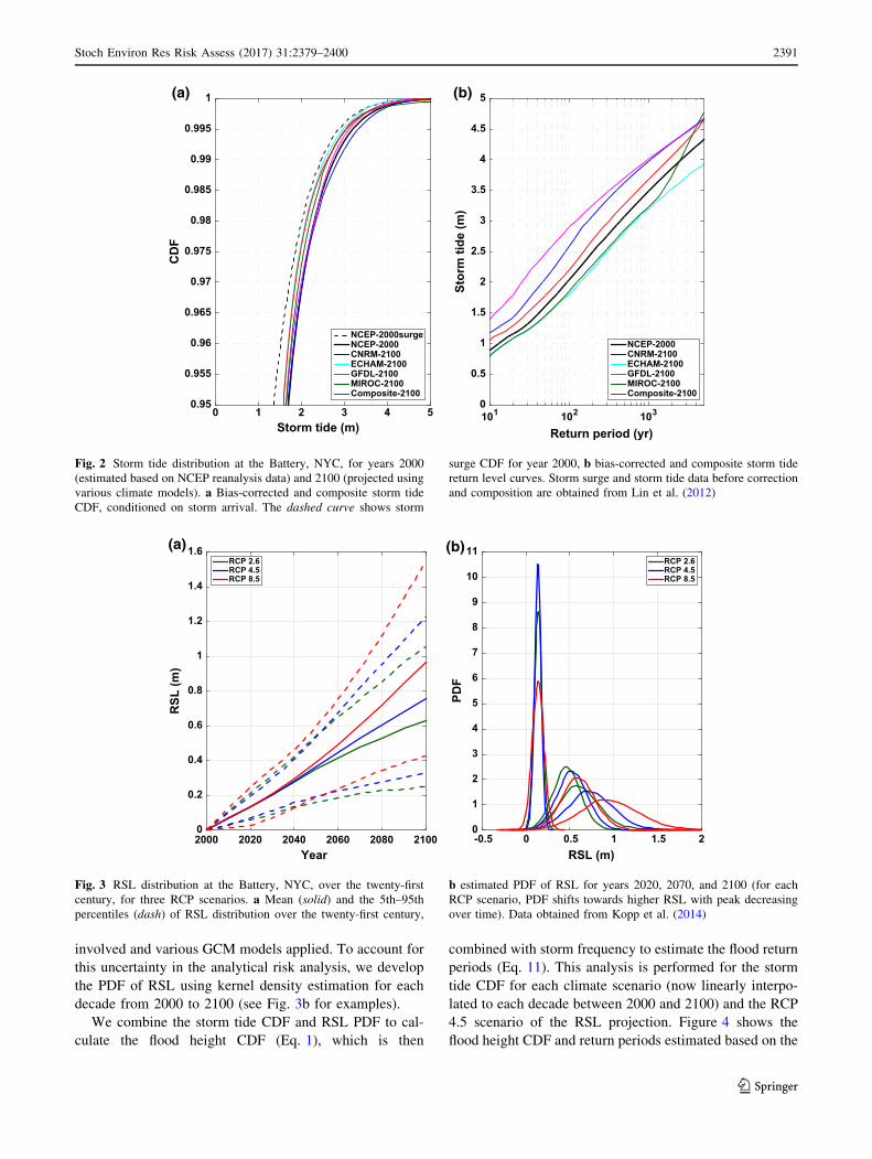
Figure 2 shows the obtained storm tide climatology

estimates at the reference location for NYC, the Battery,

for years 2000 and 2100. As it is the storm surge events

that are used for damage calculations, the storm surge CDF

for year 2000 is also shown for comparison. The difference

between the storm surge CDF and storm tide CDF for 2000

is relatively large, which indicates that the effects of

astronomical tide should not be neglected in risk analysis.

The changes of storm tide CDF between 2000 and 2100 are

relatively small for the four GCM-projections and thus for

the composite projection. However, storm tide return levels

of two out of four GCM projections for 2100 are signifi-

cantly higher than those of the NCEP 2000 reanalysis

because these two GCMs projected significant increase in

storm frequency. The other two GCMs projected slightly

lower storm frequency and also lower storm tide return

levels for 2100 compared to the NCEP 2000 reanalysis.

This comparison indicates that relatively large uncertainty

exists in climate modeling and should be accounted for in

risk assessment. While the uncertainty in storm tide esti-

mation under each climate projection is considered aleatory

as described by its probability distribution, we consider the

uncertainty in the climate projections epistemic and apply

all four available GCM projections to estimate the uncer-

tainty range around the ‘‘mean’’ composite projection.

Figure 3 shows the RSL projection at the Battery based

on Kopp et al. (2014). Over the twenty-first century, the

RSL is projected to significantly increase, by 0.63–0.97 m

for the mean, depending on the RCP scenarios (Fig. 3a).

The uncertainty of the projection, however, is large, with a

90% confidence interval of about 0.8–1.12 m around the

mean. Such a large uncertainty in RSL projection should be

accounted for in risk analysis. This uncertainty may be

considered both aleatory and epistemic as it includes

uncertainties in both the complex natural processes


123

involved and various GCM models applied. To account for

this uncertainty in the analytical risk analysis, we develop

the PDF of RSL using kernel density estimation for each

decade from 2000 to 2100 (see Fig. 3b for examples).

We combine the storm tide CDF and RSL PDF to cal-

culate the flood height CDF (Eq. 1), which is then

combined with storm frequency to estimate the flood return

periods (Eq. 11). This analysis is performed for the storm

tide CDF for each climate scenario (now linearly interpo-

lated to each decade between 2000 and 2100) and the RCP

4.5 scenario of the RSL projection. Figure 4 shows the

flood height CDF and return periods estimated based on the

Storm tide (m)0 1 2 3 4 5

CD

F

0.95

0.955

0.96

0.965

0.97

0.975

0.98

0.985

0.99

0.995

1

NCEP-2000surgeNCEP-2000CNRM-2100ECHAM-2100GFDL-2100MIROC-2100Composite-2100

Return period (yr)101 102 103

Stor

mtid

e(m

)

0

0.5

1

1.5

2

2.5

3

3.5

4

4.5

5

NCEP-2000CNRM-2100ECHAM-2100GFDL-2100MIROC-2100Composite-2100

(a) (b)

Fig. 2 Storm tide distribution at the Battery, NYC, for years 2000

(estimated based on NCEP reanalysis data) and 2100 (projected using

various climate models). a Bias-corrected and composite storm tide

CDF, conditioned on storm arrival. The dashed curve shows storm

surge CDF for year 2000, b bias-corrected and composite storm tide

return level curves. Storm surge and storm tide data before correction

and composition are obtained from Lin et al. (2012)

Year2000 2020 2040 2060 2080 2100

RSL

(m)

0

0.2

0.4

0.6

0.8

1

1.2

1.4

1.6RCP 2.6RCP 4.5RCP 8.5

RSL (m)-0.5 0 0.5 1 1.5 2

PDF

0

1

2

3

4

5

6

7

8

9

10

11RCP 2.6RCP 4.5RCP 8.5

(a) (b)

Fig. 3 RSL distribution at the Battery, NYC, over the twenty-first

century, for three RCP scenarios. a Mean (solid) and the 5th–95th

percentiles (dash) of RSL distribution over the twenty-first century,

b estimated PDF of RSL for years 2020, 2070, and 2100 (for each

RCP scenario, PDF shifts towards higher RSL with peak decreasing

over time). Data obtained from Kopp et al. (2014)


123

composite storm tide climatology. The flood hazard is

projected to increase continuously and significantly over

the twenty-first century, due to the combined effects of sea-

level rise and storm climatology change. These decadal

projections are further interpolated to yearly projections

(t = 1, 2, …, y; y = 100).

Then, we combine the hazards and vulnerability infor-

mation to estimate the damage risk for NYC. We first apply

damage analysis to both the 2000 building stock and 2040

building stock to obtain the surge damage CDF curves,

which are linearly interpolated to each year to obtain the

yearly surge damage CDF. This yearly surge damage CDF

is manipulated, according to the yearly flood height CDF

and the current surge CDF, to obtain the yearly flood

damage CDF (Eqs. 2, 3), which is combined with the storm

frequency to obtain yearly flood damage return periods

(Eq. 13). The obtained yearly flood damage CDF and

return periods, under the effects of building growth, RCP

4.5 RSL, and composite storm climatology, are shown in

Fig. 5 for each decade over the twenty-first century. The

damage return levels are projected to increase dramatically

from 2000 to 2100, due to the combined effects of all three

dynamic factors.

To better illustrate how the extreme damage levels will

increase, Fig. 6 displays the time series over the twenty-

first century of the 100-, 500-, 1000-, and 4000-year

damage levels under various combinations of the dynamic

effects, in comparison with those under the stationary

environment of year 2000 (black) (the results under certain

and various combinations of the dynamic effects are

obtained by neglecting other dynamic effects). Due to only

the building stock growth, the 100-year damage increases

slightly; however, more extreme damage levels increase

substantially, as most of the future building development is

projected by NYC-DCP to happen beyond the 100-year

flood plain. The increase of the RSL (RCP 4.5), on top of

the building growth effect, will dramatically increase the

damage at all extreme levels. The change of storm clima-

tology (composite model in this case) further increases the

extreme damage levels.

With the obtained flood damage distribution, we calcu-

late the expectation and variance of the annual damage

(Eqs. 15, 16) for each year. Under the stationary environ-

ment of year 2000, the estimated EAD is $78 million for

NYC and the estimated standard deviation of the annual

damage is much larger, at $745.3 million. Our estimation

of the EAD is higher than that obtained in Aerts et al.

(2014) of about $66.6 million (for buildings), due to three

improvements in our methodology. First, we apply statis-

tical analysis on the calculated damages to estimate the

surge damage distribution, while Aerts et al. (2014) derived

this surge damage distribution directly from the storm

surge distribution at the reference location (Battery), which

partially neglected the effect of spatial variation of the

surge. Second, we consider the effect of astronomical tide

on the damage at every surge level (Eq. 2), while Aerts

et al. (2014) approximated this effect by shifting the entire

surge distribution according to the tidal effect at a single

Flood height (m)0 1 2 3 4 5 6

CD

F

0.5

0.55

0.6

0.65

0.7

0.75

0.8

0.85

0.9

0.95

1

20002010202020302040205020602070208020902100

Return period (yr)101 102 103

Floo

dhe

ight

( m)

0

1

2

3

4

5

6

20002010202020302040205020602070208020902100

(a) (b)

Fig. 4 Flood height distribution at the Battery, NYC, years 2000–2100, based on projected RCP 4.5 RSL scenario and composite storm tide

climatology. a Flood height CDF, conditioned on storm arrival, b flood height return level curves. Results obtained from analytical analysis


123

Damage (million) ×1040 1 2 3 4 5

CD

F

0.9

0.91

0.92

0.93

0.94

0.95

0.96

0.97

0.98

0.99

1

20002010202020302040205020602070208020902100

Return period (yr)102 103

Dam

age

(mill

ion

)

×104

0

0.5

1

1.5

2

2.5

3

3.5

4

4.5

5

20002010202020302040205020602070208020902100

(a) (b)

Fig. 5 Damage distribution for NYC, years 2000–2100, based on projected building stock growth, RCP 4.5 RSL scenario, and composite storm

tide climatology. a Damage CDF, conditioned on storm arrival, b damage return level curves. Results obtained from analytical analysis

Year2000 2020 2040 2060 2080 2100

100-

yr d

amag

e (m

illio

n)

0

2000

4000

6000

8000

10000

Year2000 2020 2040 2060 2080 2100

500-

yr d

amag

e (m

illio

n)

×104

0.5

1

1.5

2

2.5

Year2000 2020 2040 2060 2080 2100

1000

-yr

dam

age

(mill

ion

)

×104

1

1.5

2

2.5

3

Year2000 2020 2040 2060 2080 2100

4000

-yr

dam

age

(mill

ion

)

×104

1.5

2

2.5

3

3.5

4

4.5

5

5.5StationaryBuildingBuilding+RSLBuilding+RSL+Composite

(a) (b)

(c) (d)

Fig. 6 Time series of various extreme damage levels for NYC, years

2000–2100, under stationary environment of year 2000 (black), non-

stationary built environment (green), non-stationary build environ-

ment and RCP 4.5 RSL (blue), and non-stationary built environment,

RCP 4.5 RSL, and composite storm tide climatology (red). a 100-yeardamage, b 500-year damage, c 1000-year damage, d 4000-year

damage. Results obtained from both analytical analysis (solid curves)

and MC simulations (dots)


123

surge level. Third, we calculate the expected total annual

damage (Eqs. 24 or 25), while Aerts et al. (2014) calcu-

lated the expected maximum annual damage (Eq. 26).

The time-varying EAD over the twenty-first century

under each and combined dynamic effects, compared to the

stationary case (black), is shown in Fig. 7. The effect of

NYC-DCP projected building stock growth is relatively

small (Fig. 7a), as expected given previous results related to

the extremes (Fig. 6). To investigate the sensitivity of the

damage risk to different RCP scenarios of the RSL, we

applied all three available RCP scenarios. As Fig. 7b shows,

although RSL is the dominant dynamic factor, the effects of

the various RCP scenarios are significantly different only in

the later decades of the twenty-first century. The EAD is

very sensitive to the variation in the storm climatology

projection, as shown in Fig. 7c, with the GFDL projection

being a case of dramatic increase of the risk (comparable to

RCP4.5 RSL) and two out of four climate-model projec-

tions (ECHAM and MIROC) being cases of slight decrease

of the risk, relative to the stationary case. The composite

storm climatology projection induces a moderate increase

in the risk, significantly lower than that of RSL but higher

than that of the building growth. Finally, under the

compound effects of all these dynamic factors (with RCP

4.5 RSL, Fig. 7d), EAD will increase nonlinearly and dra-

matically, with a large variation range due to the epistemic

uncertainty in the climate modeling of the storm climatol-

ogy. The standard deviation of the annual damage, dis-

played in Fig. 8, is also projected to increase dramatically

over the twenty-first century. The evolution pattern of the

standard deviation of the annual damage is similar to that of

the EAD, except that although ECHAM and MIROC model

projections are similar in the mean, they differ in the stan-

dard deviation of the annual damage. Also, the impact of

building growth is more substantial on the standard devia-

tion than on the mean of the annual damage.

With the obtained flood damage distribution, we also

calculate the mean of the present value of future losses

(PVL) for NYC over the twenty-first century, using the

three analytical methods discussed in Sect. 2.2.3, as shown

in Table 1. In this case study we use a discount rate of 3%

(using a higher or lower discount rate will result in a lower

or higher estimate of discounted impact of future climate

change and coastal development). Using the continuous

discounting method (Eqs. 19, 20), the mean of PVL is

about $2503 million under the stationary environment of

Year2000 2020 2040 2060 2080 2100

E[A

](m

illio

n)

0

100

200

300

400

500StationaryBuilding Growth

Year2000 2020 2040 2060 2080 2100

E[A

](m

illio

n )

0

100

200

300

400

500StationaryRCP2.6RCP4.5RCP8.5

Year2000 2020 2040 2060 2080 2100

E[A

](m

illio

n)

0

100

200

300

400

500StationaryCompositeCNRMGFDLECHAMMIROC

Year2000 2020 2040 2060 2080 2100

E[A

](m

illio

n )

0

200

400

600

800

1000

1200


(a) (b)

(c) (d)

Fig. 7 Time series of expected annual damage (EAD) for NYC,

years 2000–2100, under stationary environment of 2000 (black) and

various environmental changes. a Built environment change, b RSL

change (for three RCP scenarios), c storm climatology change (for

four GCMs and composite), d combined changes in a–c (with RCP

4.5 scenario). Results obtained from both analytical analysis (solid

curves) and MC simulations (dots; nearly indistinguishable from

analytical curves in all cases)


123

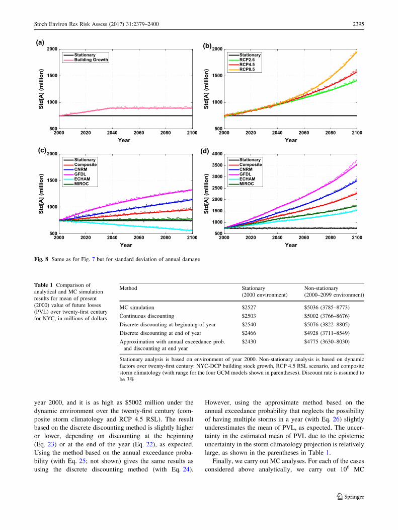
year 2000, and it is as high as $5002 million under the

dynamic environment over the twenty-first century (com-

posite storm climatology and RCP 4.5 RSL). The result

based on the discrete discounting method is slightly higher

or lower, depending on discounting at the beginning

(Eq. 23) or at the end of the year (Eq. 22), as expected.

Using the method based on the annual exceedance proba-

bility (with Eq. 25; not shown) gives the same results as

using the discrete discounting method (with Eq. 24).

However, using the approximate method based on the

annual exceedance probability that neglects the possibility

of having multiple storms in a year (with Eq. 26) slightly

underestimates the mean of PVL, as expected. The uncer-

tainty in the estimated mean of PVL due to the epistemic

uncertainty in the storm climatology projection is relatively

large, as shown in the parentheses in Table 1.

Finally, we carry out MC analyses. For each of the cases

considered above analytically, we carry out 106 MC

Table 1 Comparison of

analytical and MC simulation

results for mean of present

(2000) value of future losses

(PVL) over twenty-first century

for NYC, in millions of dollars

Method Stationary

(2000 environment)

Non-stationary

(2000–2099 environment)

MC simulation $2527 $5036 (3785–8773)

Continuous discounting $2503 $5002 (3766–8676)

Discrete discounting at beginning of year $2540 $5076 (3822–8805)

Discrete discounting at end of year $2466 $4928 (3711–8549)

Approximation with annual exceedance prob.

and discounting at end year

$2430 $4775 (3630–8030)

Stationary analysis is based on environment of year 2000. Non-stationary analysis is based on dynamic

factors over twenty-first century: NYC-DCP building stock growth, RCP 4.5 RSL scenario, and composite

storm climatology (with range for the four GCM models shown in parentheses). Discount rate is assumed to

be 3%

Year2000 2020 2040 2060 2080 2100

Std[

A](

mill

ion)

500

1000

1500


Year2000 2020 2040 2060 2080 2100

Std[

A](

mill

ion)

500

1000

1500

2000StationaryRCP2.6RCP4.5RCP8.5

Year2000 2020 2040 2060 2080 2100

Std[

A](

mill

ion)

500

1000

1500


Year2000 2020 2040 2060 2080 2100

Std[

A](

mill

ion)

500

1000

1500

2000

2500

3000

3500


(a) (b)

(c) (d)

Fig. 8 Same as for Fig. 7 but for standard deviation of annual damage


123

simulations. For the stationary environment of year 2000,

the storm arrivals are simulated as a stationary Poisson

process (Eqs. 5, 6) and the damage values are sampled

from the storm tide damage distribution for year 2000; the

MC-estimated EAD and standard deviation of the annual

damage are $78.8 and $748 million, respectively, very

close to those obtained analytically. For the dynamic

environment, the storms arrive as a non-stationary Poisson

process (Eq. 27), and the damage values are sampled from

the surge loss distribution based on the sampled arrival

time, storm tide level, and RSL (Eq. 28). As for the ana-

lytical analysis, the cases of certain and combinations of

the dynamic effects are obtained by neglecting other

dynamic effects. The obtained MC estimation of the time-

varying mean and standard deviation of the annual damage

are very close to the analytical results for all cases (Figs. 7,

8), except that the MC-estimated standard deviation of the

annual damage is slightly higher than the analytical values

for the very extremes (Fig. 8d), perhaps due to slight

different numerical approximations applied towards the

limit of the available data. The MC-estimated extreme

damage levels compare also very closely with the analyt-

ical results (Fig. 6); the fluctuations of MC estimations

around the analytical estimations indicate that an extremely

large number of simulations would be needed to achieve

convergence in the estimation for the very end of the tail of

the damage risk. In addition, the MC-estimated mean val-

ues of PVL (calculated using Eq. 17) come very close to

the analytical results (Table 1), especially those calculated

with the continuous discounting method as the MC method

considers the storm arrival time within the year.

Analytical methods are simpler and more efficient and

thus should be used whenever possible, as explored in this

study. MC simulations, after being validated with the

analytical results, can be applied to estimate more complex

risk measures. We use the MC samples that are validated

for both the mean and extreme damage measures (Figs. 6,

7, 8; Table 1) to estimate the probability distribution of

PVL (million)

0 5000 10000 15000

PD

F×10-4

0

1

2

3

4

5


PVL (million)0 5000 10000 15000

PD

F

×10-4

0

1

2

3

4

5

6StationaryRCP 2.6RCP 4.5RCP 8.5

PVL (million)

0 5000 10000 15000

PD

F

×10-4

0

1

2

3

4

5


PVL (million)0 5000 10000 15000

PD

F

×10-4

0

1

2

3

4

5


(a) (b)

(c) (d)

Fig. 9 PDF of present (2000) value of future losses (PVL) over the

twenty-first century for NYC, under stationary environment of 2000

(black) and various environmental changes. a Built environment

change, b RSL change (for three RCP scenarios), c storm climatology

change (for four GCMs and composite), d combined changes in a–c (with RCP 4.5 scenario). Discount rate is assumed to be 3%. Results

obtained from MC simulations


123

PVL. The obtained PDF of PVL (using the nonparametric

density method) is displayed in Fig. 9, with representative

statistics shown in Table 2.

For the stationary case, the standard deviation of PVL is

about 1.2 times the mean, the median is about 0.6 times the

mean, and the 95th percentile is about 3.3 times the mean.

The effects of the dynamic factors on the overall, tempo-

rally integrated damage risk is indicated by the widening

and shifting of the PDF of PVL to larger damage values. As

expected, the effect of building stock growth is relatively

small. The effect of RSL is dominant but is not very sen-

sitive to the RCP emission scenarios, because the difference

of the RCPs is largely shown in the later decades (Figs. 7,

8), when the discounting is larger. The effect of storm cli-

matology change shows a small to moderate effect when

measured by the composite climate, while large variations

exist among the GCM projections even for the same

emission scenario (A1B). In the extreme case (GFDL), the

effect of storm climatology is larger than the effect of RSL

on all PVL levels (see Table 2). Finally, the compound

effects of the three dynamic factors would greatly shift the

PDF of the PVL. Compared to the stationary case, if all

three non-stationary effects are considered with the com-

posite storm climate and RCP 4.5 RSL (the four GCM storm

climates and RCP 4.5 RSL), the mean of PVL is estimated

to increase by 2.0 (1.5–3.5) times, the standard deviation

increase by 1.3 (1.2–1.7) times, the median increase by 2.7

(1.8–5.3) times, and the 95th percentile increase by 1.6

(1.3–2.2) times. Thus, the change in the dynamic risk is

apparent not only in the mean but also in the entire distri-

bution of the PVL. Considering the PDF of PVL rather than

only the mean is a more comprehensive approach to eval-

uate the overall flood damage risk as well as the benefit of

risk mitigation strategies (Part II).

4 Summary

We have proposed an integrated dynamic risk analysis for

flooding task (iDraft) framework for estimating the storm

surge flood damage risk at regional scales, considering

integrated dynamic effects of storm climatology change,

sea-level rise, and coastal development, in a formal,

coherent Poisson-process framework. It is shown that

various time-varying risk metrics of interest, such as the

return period of various damage levels and the mean and

variance of annual damage, can be derived analytically, as

well as the mean of the present value of future losses

(PVL). However, risk measures that involve temporal

integration of the stochastic process, such as the probability

distribution of PVL, may be difficult or impossible to

derive analytically. MC methods are thus developed to

estimate such risk measures. The analytical and MCTable

2Mean;standarddeviation;median;and75th,95th,and99th

percentilesofpresent(2000)valueoffuture

losses

(PVL)over

twenty-firstcentury

forNYC,in

millionsofdollars,based

onMC

simulations(asin

Fig.9)

Effects

Mean

SD

Median

75th

95th

99th

Stationary(Fig.9)

$2527

$3073

$1430

$2968

$8323

$15,238

Building(Fig.9a)

$2764

$3315

$1559

$3315

$9096

$16,356

RSL(Fig.9b)

$3791(3685–4046)

$3502(3501–3600)

$2675(2548–2935)

$4683(4555–5041)

$10,466(10,359–10,897)

$17,505(17,449–17,985)

Storm

(Fig.9c)

$2891(2307–4549)

$3241(2961–3686)

$1754(1252–3429)

$3457(2627–5636)

$8993(7839–11,587)

$16,090(14,704–18,723)

Combined

(Fig.9d)

$5036(3785–8773)

$4130(3646–5203)

$3793(2578–7557)

$6318(4677–10,979)

$12,903(10,752–18,510)

$20,814(18,198–26,742)

Discountrateisassumed

tobe3%.ConsistentwithFig.9,forRSLanalysis,reported

values

areforRCP4.5

scenario,withvalues

inparentheses

showingrangeforRCP2.6

and8.5

scenarios.

Forstorm

clim

atologychangeanalysis,reported

values

areforcomposite

clim

ateprojection,withvalues

inparentheses

showingrangeforthefourclim

atemodel

projections.Foranalysisof

combined

dynam

iceffects,

reported

values

areforcomposite

storm

clim

atologyprojection(w

ithRCP4.5

scenario),withvalues

inparentheses

showingrangeforthefourclim

atemodel

projectionsofstorm

clim

atology(w

ithRCP4.5

scenario)


123

methods are theoretically consistent and validate each other

in the complex flood risk analysis task. The iDraft frame-

work should be extended to consider extratropical cyclone

surge hazards in addition to tropical cyclone surge hazards

and social vulnerability in addition to physical vulnera-

bility of coastal cities.

Although the discrete storm surge events can be rea-

sonably considered as conditionally independent, the con-

tinuous RSL is temporally correlated. Future analysis on

the correlation of RSL is useful, e.g., for analytically

estimating the variance of PVL and perhaps the probability

distribution of PVL. When applying climate-model pro-

jected storm surge/tide climatology to flood hazard and

damage risk analysis, the climate-model bias may be rel-

atively large and should be first corrected. Also, multiple

model projections may be combined to obtain a weighted

average or ‘‘best’’ climate projection. However, the specific

methods of climate-model bias correction and model

combination needs to be further developed. Given the

estimated flood as a combination of RSL and storm tide,

inundation over land can be better modeled with dynamic

modeling than static mapping, especially for areas with

complex topography. The effect of natural and built flood

defense is grossly approximated here; it warrants better

consideration in future studies. Vulnerability models that

account for effects of not only still water inundation but

also dynamic wave impact can more realistically represent

damage mechanisms and thus should be developed and

applied in the future. These modeling improvements may

significantly reduce the epistemic uncertainties in flood risk

assessment. In addition, PVL can be very sensitive to the

discount rate applied, which should be considered carefully

in risk management applications.

The case study for NYC shows that the impact of pop-

ulation growth and coastal development on future damage

risk is likely to be small compared to climate change fac-

tors, because the city is already heavily built especially at

the coastal front. Sea-level rise will significantly increase

the damage risk even under the most stringent emission

scenario. Storm surges will likely intensify and/or become

more frequent, further increasing the flood risk and espe-

cially associated uncertainty. The joint effect of coastal

development, sea-level rise, and storm climatology change

is possibly a dramatic increase of the risk over the twenty-

first century and a significant shift of the temporally inte-

grated losses towards high values. Part II of this study will

evaluate the cost-effectiveness of various flood mitigation

strategies proposed for NYC to avert the potential impact

of climate change.

Acknowledgements We acknowledge the support of National Sci-

ence Foundation Grant EAR-1520683. We thank Hans de Moel of

VU University, Netherlands, for providing us with inundation maps

and building stock data. We thank Robert Kopp of Rutgers Univer-

sity, USA, for kindly making the RSL projection available. We also

thank two anonymous reviewers for their valuable comments.

Open Access This article is distributed under the terms of the Creative

Commons Attribution 4.0 International License (http://creative

commons.org/licenses/by/4.0/), which permits unrestricted use, dis-

tribution, and reproduction in any medium, provided you give

appropriate credit to the original author(s) and the source, provide a link

to the Creative Commons license, and indicate if changes were made.

References

Aerts JCJH, Lin N, Botzen W, Emanuel K, de Moel H (2013) Low-

probability flood risk modeling for New York City. Risk Anal

33(5):772–788. doi:10.1111/risa.12008

Aerts JCJH, Botzen WJW, Emanuel K, Lin N, de Moel H, Michel-

Kerjan EO (2014) Evaluating flood resilience strategies for

coastal megacities. Science 344(6183):473–475. doi:10.1126/

science.1248222

Applied Research Associates (ARA) (2007) Level 2 exposure data

compilation for New York City office of emergency manage-

ment. Prepared for National Institute of Building Sciences. ARA,

Albuquerque, NM

Bender MA, Knutson TR, Tuleya RE, Sirutis JJ, Vecchi GA, Garner

ST, Held IM (2010) Modeled impact of anthropogenic warming

on the frequency of intense Atlantic hurricanes. Science

327(5964):454–458. doi:10.1126/science.1180568

Bouwer LM (2013) Projections of future extreme weather losses

under changes in climate and exposure. Risk Anal

33(5):915–930. doi:10.1111/j.1539-6924.2012.01880.x

Buchanan MK, Kopp RE, Oppenheimer M, Tebaldi C (2015)

Allowances for evolving coastal flood risk under uncertain local

sea-level rise. Clim Change 137(3–4):347–362. doi:10.1007/

s10584-016-1664-7

Colle BA, Buonaiuto F, Bowman MJ, Wilson RE, Flood R, Hunter R,

Mintz A, Hill D (2010) New York City’s vulnerability to coastal

flooding. Bull Am Meteorol Soc 89(6):829–841. doi:10.1175/

2007BAMS2401.1

Colle BA, Booth JF, Chang EKM (2015) A review of historical and

future changes of extratropical cyclones and associated impacts

along the US east coast. Curr Clim Change Rep 1(3):125–143.

doi:10.1007/s40641-015-0013-7

Curtis KJ, Schneider A (2011) Understanding the demographic

implications of climate change: estimates of localized population

predictions under future scenarios of sea-level rise. Popul

Environ 33(1):28–54. doi:10.1007/s11111-011-0136-2

Cutter SL, Mitchell JT, Scott MS (2000) Revealing the vulnerability

of people and places: a case study of Georgetown County, South

Carolina. Ann Assoc Am Geogr 90(4):713–737. doi:10.1111/

0004-5608.00219

Czajkowski J, Kunreuther H, Michel-Kerjan E (2013) Quantifying

riverine and storm-surge flood risk by single-family residence:

application to Texas. Risk Anal 33(12):2092–2110. doi:10.1111/

risa.12068

Ellingwood BR, Lee JY (2016) Managing risks to civil infrastructure

due to natural hazards: communicating long-term risks due to

climate change. In: Risk analysis of natural hazards. Springer,

Berlin, pp 97–112

Elsner JB, Bossak BH (2001) Bayesian analysis of U.S. hurricane

climate. J Clim 14:4341–4350. doi:10.1175/1520-

0442(2001)014\4341:BAOUSH[2.0.CO;2

Emanuel KA (2013) Downscaling CMIP5 climate models shows

increased tropical cyclone activity over the 21st century. Proc


123

http://creativecommons.org/licenses/by/4.0/

http://creativecommons.org/licenses/by/4.0/

http://dx.doi.org/10.1111/risa.12008

http://dx.doi.org/10.1126/science.1248222



http://dx.doi.org/10.1111/j.1539-6924.2012.01880.x

http://dx.doi.org/10.1007/s10584-016-1664-7

http://dx.doi.org/10.1007/s10584-016-1664-7

http://dx.doi.org/10.1175/2007BAMS2401.1

http://dx.doi.org/10.1175/2007BAMS2401.1

http://dx.doi.org/10.1007/s40641-015-0013-7

http://dx.doi.org/10.1007/s11111-011-0136-2

http://dx.doi.org/10.1111/0004-5608.00219

http://dx.doi.org/10.1111/0004-5608.00219



http://dx.doi.org/10.1175/1520-0442(2001)014%3c4341:BAOUSH%3e2.0.CO;2

http://dx.doi.org/10.1175/1520-0442(2001)014%3c4341:BAOUSH%3e2.0.CO;2

Natl Acad Sci 110(30):12219–12224. doi:10.1073/pnas.

1301293110

Emanuel K, Ravela S, Vivant E, Risi C (2006) A statistical

deterministic approach to Hurricane risk assessment. Bull Am

Meteorol Soc 87(3):299–314. doi:10.1175/BAMS-87-3-299

Emanuel K, Sundararajan R, Williams J (2008) Hurricanes and global

warming: results from downscaling IPCC AR4 simulations. Bull

Am Meteorol Soc 89(3):347–367. doi:10.1175/BAMS-89-3-347

FEMA (2009) Federal Emergency Management Agency, ‘‘HAZUS-

MH MR4 flood model technical manual’’. FEMA, Washington.

https://www.fema.gov/media-library/assets/documents/24609

Ge Y, Dou W, Gu Z, Qian X, Wang J, Xu W, Shi P, Ming X, Zhou X,

Chen Y (2013) Assessment of social vulnerability to natural

hazards in the Yangtze River Delta, China. Stoch Environ Res

Risk Assess 27(8):1899–1908. doi:10.1007/s00477-013-0725-y

Gornitz V, Couch S, Hartig EK (2001) Impacts of sea level rise in the

New York City metropolitan area. Glob Planet Change

32(1):61–88. doi:10.1016/S0921-8181(01)00150-3

Grossi P, Kunreuther H, Windeler D (2005) An introduction to

catastrophe models and insurance. In: Catastrophe modeling: a

new approach to managing risk. Springer, New York, pp 23–42

Hall J, Solomatine D (2008) A framework for uncertainty analysis in

flood risk management decisions. Int J River Basin Manag

6(2):85–98. doi:10.1080/15715124.2008.9635339

Hall T, Yonekura E (2013) North American tropical cyclone landfall

and SST: a statistical model study. J Clim. doi:10.1175/JCLI-D-

12-00756.1

Hall JW, Sayers PB, Dawson RJ (2005) National-scale assessment of

current and future flood risk in England and Wales. Nat Hazards

36(1–2):147–164. doi:10.1007/s11069-004-4546-7

Hallegatte S, Henriet F, Corfee-Morlot J (2010) The economics of

climate change impacts and policy benefits at city scale: a

conceptual framework. Clim Change 104(1):51–87. doi:10.1007/

s10584-010-9976-5

Hallegatte S, Ranger N, Mestre O, Dumas P (2011) Assessing climate

change impacts, sea level rise and storm surge risk in port cities:

a case study on Copenhagen. Clim Change 104(1):113–137.

doi:10.1007/s10584-010-9978-3

Hinkel J, Lincke D, Vafeidis AT, Perrette M, Nicholls RJ, Tol RSJ,

Marzeion B, Fettweis X, Ionescu C, Levermann A (2014)

Coastal flood damage and adaptation costs under 21st century

sea-level rise. Proc Natl Acad Sci 111(9):3292–3297. doi:10.

1073/pnas.1222469111

Hoffman RN, Dailey P, Hopsch S, Ponte RM, Quinn K, Hill EM,

Zachry B (2011) An estimate of increases in storm surge risk to

property from sea level rise in the first half of the twenty-first

century. Weather Clim Soc 2(4):271–293. doi:10.1175/

2010WCAS1050.1

Houston JR (2013) Methodology for combining coastal design-flood

levels and sea-level rise projections. J Waterw Port Coast Ocean

Eng 139(5):341–345. doi:10.1061/(ASCE)WW.1943-5460.

0000194

Hunter JR, Church JA, White NJ, Zhang X (2013) Towards a global

regionally varying allowance for sea-level rise. Ocean Eng

71(October):17–27. doi:10.1016/j.oceaneng.2012.12.041

Jain VK, Davidson R, Rosowsky D (2005) Modeling changes in

hurricane risk over time. Nat Hazards Rev 6(2):88–96. doi:10.

1061/(ASCE)1527-6988(2005)6:2(88)

Jelesnianski CP, Chen J, Shaffer WA (1992), SLOSH: sea, lake, and

overland surges from hurricanes, NOAA Technical Report.

NWS 48, NOAA/AOML Library, Miami

Kleinosky LR, Yarnal B, Fisher A (2006) Vulnerability of Hampton

Roads, Virginia to storm-surge flooding and sea-level rise. Nat

Hazards 40(1):43–70. doi:10.1007/s11069-006-0004-z

Klima K, Lin N, Emanuel K, Morgan MG, Grossmann I (2012)

Hurricane modification and adaptation in Miami-Dade county,

Florida. Environ Sci Technol 46(2):636–642. doi:10.1021/

es202640p

Knutson TR, McBride JL, Chan J, Emanuel K, Holland G, Landsea C,

Held I, Kossin JP, Srivastava AK, Sugi M (2010) Tropical

cyclones and climate change. Nat Geosci 3(3):157–163. doi:10.

1038/ngeo779

Knutson TR, Sirutis JJ, Vecchi GA, Garner S, Zhao M, Kim H-S,

Bender M, Tuleya RE, Held IM, Villarini G (2013) Dynamical

downscaling projections of twenty-first-century Atlantic hurri-

cane activity: CMIP3 and CMIP5 model-based scenarios. J Clim

26(17):6591–6617. doi:10.1175/JCLI-D-12-00539.1

Knutson TR, Sirutis JJ, Zhao M, Tuleya RE, Bender M, Vecchi GA,

Villarini G, Chavas D (2015) Global projections of intense

tropical cyclone activity for the late twenty-first century from

dynamical downscaling of CMIP5/RCP4.5 scenarios. J Clim

28(18):7203–7224. doi:10.1175/JCLI-D-15-0129.1

Kopp RE, Horton RM, Little CM, Mitrovica JX, Oppenheimer M,

Rasmussen DJ, Strauss BH, Tebaldi C (2014) Probabilistic 21st

and 22nd century sea-level projections at a global network of

tide-gauge sites. Earths Future 2(8):383–406. doi:10.1002/

2014EF000239

Lee JY, Ellingwood BR (2015) Ethical discounting for civil

infrastructure decisions extending over multiple generations.

Struct Saf 57:43–52. doi:10.1016/j.strusafe.2015.06.001

Lickley MJ, Lin N, Jacoby HD (2014) Analysis of coastal protection

under rising flood risk. Clim Risk Manag 6:18–26. doi:10.1016/j.

crm.2015.01.001

Lin N (2015) An integrated approach to assess and manage hurricane

risk in a changing climate. The Bridge, no. Winter 2015,

pp 45–51

Lin N, Emanuel K (2016) Grey swan tropical cyclones. Nat Clim

Change 6(1):106–111. doi:10.1038/nclimate2777

Lin N, Emanuel KA, Smith JA, Vanmarcke E (2010) Risk assessment

of hurricane storm surge for New York City. J Geophys Res

115(D18):D18121. doi:10.1029/2009JD013630

Lin N, Emanuel K, Oppenheimer M, Vanmarcke E (2012) Physically

based assessment of hurricane surge threat under climate change.

Nat Clim Change 2(6):462–467. doi:10.1038/nclimate1389

Lin N, Lane P, Emanuel KA, Sullivan RM, Donnelly JP (2014)

Heightened hurricane surge risk in northwest Florida revealed

from climatological-hydrodynamic modeling and paleorecord

reconstruction. J Geophys Res Atmos 119(14):8606–8623.

doi:10.1002/2014JD021584

Lin N, Kopp RE, Horton BP, Donnelly JP (2016) Hurricane Sandy’s

flood frequency increasing from year 1800 to 2100. Proc Natl

Acad Sci. doi:10.1073/pnas.1604386113

Little CM, Horton RM, Kopp RE, Oppenheimer M, Vecchi GA,

Villarini G (2015) Joint projections of US East Coast sea level

and storm surge. Nat Clim Change 5(12):1114–1120. doi:10.

1038/nclimate2801

Meinshausen M, Smith SJ, Calvin K, Daniel JS, Kainuma MLT,

Lamarque J-F, Matsumoto K et al (2011) The RCP greenhouse

gas concentrations and their extensions from 1765 to 2300. Clim

Change 109(1–2):213–241. doi:10.1007/s10584-011-0156-z

Mendelsohn R, Emanuel K, Chonabayashi S, Bakkensen L (2012) The

impact of climate change on global tropical cyclone damage. Nat

Clim Change 2(3):205–209. doi:10.1038/nclimate1357

Mudd L, Wang Y, Letchford C, Rosowsky D (2014) Hurricane wind

hazard assessment for a rapidly warming climate scenario.

J Wind Eng Ind Aerodyn 133(October):242–249. doi:10.1016/j.

jweia.2014.07.005

Murakami H, Vecchi GA, Underwood S, Delworth TL, Wittenberg

AT, Anderson WG, Chen J-H et al (2015) Simulation and

prediction of category 4 and 5 hurricanes in the high-resolution

GFDL HiFLOR coupled climate model*. J Clim

28(23):9058–9079. doi:10.1175/JCLI-D-15-0216.1


123

http://dx.doi.org/10.1073/pnas.1301293110


http://dx.doi.org/10.1175/BAMS-87-3-299

http://dx.doi.org/10.1175/BAMS-89-3-347

https://www.fema.gov/media-library/assets/documents/24609

http://dx.doi.org/10.1007/s00477-013-0725-y

http://dx.doi.org/10.1016/S0921-8181(01)00150-3

http://dx.doi.org/10.1080/15715124.2008.9635339

http://dx.doi.org/10.1175/JCLI-D-12-00756.1


http://dx.doi.org/10.1007/s11069-004-4546-7

http://dx.doi.org/10.1007/s10584-010-9976-5

http://dx.doi.org/10.1007/s10584-010-9976-5

http://dx.doi.org/10.1007/s10584-010-9978-3



http://dx.doi.org/10.1175/2010WCAS1050.1

http://dx.doi.org/10.1175/2010WCAS1050.1

http://dx.doi.org/10.1061/(ASCE)WW.1943-5460.0000194

http://dx.doi.org/10.1061/(ASCE)WW.1943-5460.0000194

http://dx.doi.org/10.1016/j.oceaneng.2012.12.041

http://dx.doi.org/10.1061/(ASCE)1527-6988(2005)6:2(88)


http://dx.doi.org/10.1007/s11069-006-0004-z

http://dx.doi.org/10.1021/es202640p

http://dx.doi.org/10.1021/es202640p

http://dx.doi.org/10.1038/ngeo779

http://dx.doi.org/10.1038/ngeo779



http://dx.doi.org/10.1002/2014EF000239

http://dx.doi.org/10.1002/2014EF000239

http://dx.doi.org/10.1016/j.strusafe.2015.06.001

http://dx.doi.org/10.1016/j.crm.2015.01.001

http://dx.doi.org/10.1016/j.crm.2015.01.001

http://dx.doi.org/10.1038/nclimate2777

http://dx.doi.org/10.1029/2009JD013630


http://dx.doi.org/10.1002/2014JD021584




http://dx.doi.org/10.1007/s10584-011-0156-z


http://dx.doi.org/10.1016/j.jweia.2014.07.005

http://dx.doi.org/10.1016/j.jweia.2014.07.005


National Research Council (NRC) (2014) Reducing coastal risk on

the East and Gulf Coasts. The National Academies Press,

Washington, D.C. http://citeseerx.ist.psu.edu/viewdoc/down

load?doi=10.1.1.694.6940&rep=rep1&type=pdf

Nicholls RJ, Cazenave A (2010) Sea-level rise and its impact on

coastal zones. Science 328(5985):1517–1520. doi:10.1126/

science.1185782

Nicholls RJ, Tol RSJ (2006) Impacts and responses to sea-level rise: a

global analysis of the SRES scenarios over the twenty-first

century. Philos Trans R Soc Lond A Math Phys Eng Sci

364(1841):1073–1095. doi:10.1098/rsta.2006.1754

Onof C, Chandler RE, Kakou A, Northrop P, Wheater HS, Isham V

(2000) Rainfall modelling using Poisson-cluster processes: a

review of developments. Stoch Environ Res Risk Assess

14(6):384–411. doi:10.1007/s004770000043

Orton P, Vinogradov S, Georgas N, Blumberg A, Lin N, Gornitz V,

Little C, Jacob K, Horton R (2015) New York City panel on

climate change 2015 report chapter 4: dynamic coastal flood

modeling. Ann N Y Acad Sci 1336(1):56–66. doi:10.1111/nyas.

12589

Ou-Yang C, Kunreuther H (2013) An economic analysis of climate

adaptations to hurricane risk in St. Lucia. Geneva Pap Risk Insur

Issues Pract 38(3):521–546. doi:10.1057/gpp.2013.18

Ramirez JA, Lichter M, Coulthard TJ, Skinner C (2016) Hyper-

resolution mapping of regional storm surge and tide flooding:

comparison of static and dynamic models. Nat Hazards

82(1):571–590. doi:10.1007/s11069-016-2198-z

Reed AJ, Mann ME, Emanuel KA, Lin N, Horton BP, Kemp AC,

Donnelly JP (2015) Increased threat of tropical cyclones and

coastal flooding to New York City during the anthropogenic era.

Proc Natl Acad Sci 112(41):12610–12615. doi:10.1073/pnas.

1513127112

Rosenzweig C, Solecki W (2014) Hurricane Sandy and adaptation

pathways in New York: lessons from a first-responder city. Glob

Environ Change 28(September):395–408. doi:10.1016/j.gloenv

cha.2014.05.003

Tebaldi C, Strauss BH, Zervas CE (2012) Modelling sea level rise

impacts on storm surges along US coasts. Environ Res Lett

7(1):014032. doi:10.1088/1748-9326/7/1/014032

Tol RSJ (2002a) Estimates of the damage costs of climate change.

Part 1: benchmark estimates. Environ Resour Econ 21(1):47–73.

doi:10.1023/A:1014500930521

Tol RSJ (2002b) Estimates of the damage costs of climate change,

part II. Dynamic estimates. Environ Resour Econ 21(2):135–160.

doi:10.1023/A:1014539414591

Vanem E (2011) Long-term time-dependent stochastic modelling of

extreme waves. Stoch Environ Res Risk Assess 25(2):185–209.

doi:10.1007/s00477-010-0431-y

Vickery PJ, Wadhera D, Twisdale LA Jr., Lavelle FM (2009) U.S.

hurricane wind speed risk and uncertainty. J Struct Eng

135(3):301–320. doi:10.1061/(ASCE)0733-9445(2009)135:

3(301)

Westerink JJ, Luettich RA, Feyen JC, Atkinson JH, Dawson C,

Roberts HJ, Powell MD, Dunion JP, Kubatko EJ, Pourtaheri H

(2008) A basin- to channel-scale unstructured grid hurricane

storm surge model applied to southern Louisiana. Mon Weather

Rev 136(3):833–864. doi:10.1175/2007MWR1946.1

Wood RM, Drayton M, Berger A, Burgess P, Wright T (2005)

Catastrophe loss modelling of storm-surge flood risk in eastern

England. Philos Trans R Soci Lond A Math Phys Eng Sci

363(1831):1407–1422. doi:10.1098/rsta.2005.1575

Wu SY, Yarnal B, Fisher A (2002) Vulnerability of coastal

communities to sea-level rise: a case study of Cape May County,

New Jersey, USA. Clim Res 22:255–270. doi:10.3354/cr022255

Wu S, Feng A, Gao J, Chen M, Li Y, Wang L (2016) Shortening the

recurrence periods of extreme water levels under future sea-level

rise. Stoch Environ Res Risk Assess 1–12. doi:10.1007/s00477-

016-1327-2

Yin J, Lin N, Yu D (2016) Coupled modeling of storm surge and

coastal inundation: a case study in New York City during

Hurricane Sandy. Water Resour Res 52:8685–8699. doi:10.1002/

2016WR019102


123

http://citeseerx.ist.psu.edu/viewdoc/download%3fdoi=10.1.1.694.6940%26rep=rep1%26type=pdf

http://citeseerx.ist.psu.edu/viewdoc/download%3fdoi=10.1.1.694.6940%26rep=rep1%26type=pdf



http://dx.doi.org/10.1098/rsta.2006.1754

http://dx.doi.org/10.1007/s004770000043

http://dx.doi.org/10.1111/nyas.12589

http://dx.doi.org/10.1111/nyas.12589

http://dx.doi.org/10.1057/gpp.2013.18

http://dx.doi.org/10.1007/s11069-016-2198-z



http://dx.doi.org/10.1016/j.gloenvcha.2014.05.003

http://dx.doi.org/10.1016/j.gloenvcha.2014.05.003

http://dx.doi.org/10.1088/1748-9326/7/1/014032

http://dx.doi.org/10.1023/A:1014500930521

http://dx.doi.org/10.1023/A:1014539414591

http://dx.doi.org/10.1007/s00477-010-0431-y



http://dx.doi.org/10.1175/2007MWR1946.1

http://dx.doi.org/10.1098/rsta.2005.1575

http://dx.doi.org/10.3354/cr022255

http://dx.doi.org/10.1007/s00477-016-1327-2

http://dx.doi.org/10.1007/s00477-016-1327-2

http://dx.doi.org/10.1002/2016WR019102

http://dx.doi.org/10.1002/2016WR019102

Dealing with hurricane surge flooding in a changing ...

Documents

Transcript of Dealing with hurricane surge flooding in a changing ...