De-embedding and other SDLA – Serial Data Link …€“ the fixture with dip can be used ...

De-embedding and other SDLA – Serial Data Link Analysis for High Speed Serial StandardsOptional segment on 10/25/40 Gb/s Optical Ethernet

2

Agenda

De-embedding Primer

the Electrical SERDES measurement challengean example at 25 Gb/s

Fast Optical Signals – new developments

SDLA Beyond de-embedding

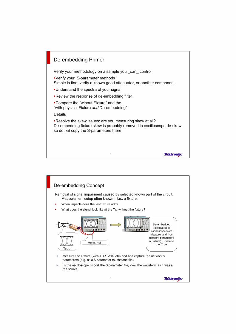
De-embedding Primer

Verify your methodology on a sample you _can_ control

Verify your S-parameter methods Simple is fine: verify a known good attenuator, or another component

Understand the spectra of your signal

Review the response of de-embedding filter

Compare the “wihout Fixture” and the“with physical Fixture and De-embedding”

Details

Resolve the skew issues: are you measuring skew at all?De-embedding fixture skew is probably removed in oscilloscope de-skew, so do not copy the S-parameters there

3

44

De-embedding Concept

Removal of signal impairment caused by selected known part of the circuit. Measurement setup often known – i.e., a fixture.

When impacts does the test fixture add?

What does the signal look like at the Tx, without the fixture?

Measure the Fixture (with TDR, VNA, etc) and and capture the network’s parameters (e.g. as a S parameter touchstone file)

► In the oscilloscope Import the S parameter file, view the waveform as it was at the source.

+

-

+

- Fixture

Measured

De-embedded (calculated in

oscilloscope from ‘Measure’ and from network parameters of fixture)… close to

the ‘True’

True

De-embedding defined

We can calculate at the waveform at Desired plane:

+

-

+

-

+

-P

re-E

mp

has

is

+

-

+

- Fixture

DesiredPlane, S(s)

AcquisitionPlane, R(s)

Transfer,H(s)

)(

)()(

sH

sRsS

We can measure at the Acquisition plane.

We want to see at theDesired Plane, S(s) …

(or, de-convolve in time-domain)

Looks simple?

It is not as simple as it looks; some effort is needed.

5

6

De-embedding Considerations:

Successful de-embedding starts with good quality Fixture board design data

– Matched impedance, low loss structures– No gain– No significant resonances– No large dips

5 GHz 10 GHz

We can calculate at the waveform at Desired plane:)(

)()(

sH

sRsS

What will the denominator do?What can we do to avoid this problem.

7

De-embedding Considerations:

Successful de-embedding starts with good quality Fixture board design data

– Matched impedance, low loss structures– No gain– No significant resonances– No large dips

Quality S-Parameter measurement– “How much BW is needed” turns out to be:– How do you cover your harmonics?

Typically 3rd or 5th harmonic is needed in recovered signal well… depending wheateryou are working on chip characterization or on system verification.

– How do you now what’s in your signal?Oscilloscope offers some support for fft.

– Verify it!

5 GHz 10 GHz

How much S-parameters do you need?

Experiment with a signal from BERT might not be a typical case

No SERDES has this much HF

S-parameters willhave to be accurateto what frequency?

How to perform thetest better?

8

How much S-parameters do you need?

Opposite problem: spectra of a 1st generation device is very limited.

Is it o.k. no device will have 3rd harmonic?How about in5 years, after twoprocess shrinks?

9

10

De-embedding Considerations:Back to the ‘dip’

With information about the design in hand you can decide if

– the fixture with dip can be used …(left pic)

– Can not be used and must be redesigned(right picture)

So don’t just rely on the automaticthreshold; verify its decision with yourdesign knowledge…and do custom ifneeded

5 GHz 10 GHz

Define custom bandwidth for de-embedding 1

The de-embedding tool for SDLA for RTO (Sampling is similar) is below.

Note on bottom right the ‘Custom’ button; if you use it you will have the choice of …

11

Define custom bandwidth for de-embedding 2

You will have the choice of BW at which to limit the de-embedding process

Also in case of Sampling you can manipulate the floor.

Note that the filter is not vere sharp – why is that?

12

Compare the “without Fixture” and the“with physical Fixture and De-embedding”

Verify the parameters of the two eye diagrams, the– “without Fixture”

and the– “with physical Fixture and De-embedding”

What to compare:– Jitter: DDJ, RJ, TJ

BUT!Note that for a device with flat group delay the result tends to always be good (since not much DDJ is generated). So this might be a very easy measure… too easy to accept. So:

– Vertical: also measure vertical eye amplitude, vertical eye closure, if possible vertical eye opening @BER

If you like the result, use de-embedding

If you don’t like the result – work the methodology till the result is acceptable.

13

Fixture Skew

If your Data and Data_ fixture signal path have skew:Do we always want to de-embed this Fixture Skew?

– Perhaps… but ONLY ONCE.Do not remove the fixture skew in two places.That is, do NOT do it in both your de-embedding and in your oscilloscope Deskew

If you will De-skew your oscilloscope for minimum skew at the time of measurement through the fixture…

then supply the S-parameters with the skew removed– You can do this IF Data and Data_ are NOT coupled (e.g. coax Cable)– When measuring DUT through TDT response, de-skew for minimum

skew.– Derived S21 will describe the Cable + De-skewed oscilloscope.

And remember: if the skew is insignificant, don’t bother. You don’t have to do everything; only what matters.

14

Let’s review again our…Step by Step De-embedding guide






Details


Questions?

15

Practical Example:PCIe at 8 Gb/s






Details


Questions?

16

17

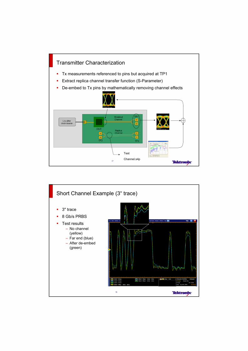
Tx measurements referenced to pins but acquired at TP1

Extract replica channel transfer function (S-Parameter)

De-embed to Tx pins by mathematically removing channel effects

Transmitter Characterization

Test

Channel.s4p

18

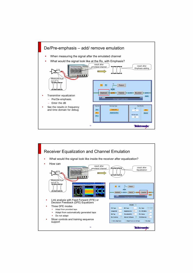
Short Channel Example (3“ trace)

3" trace

8 Gb/s PRBS

Test results– No channel

(yellow)– Far end (blue)– After de-embed

(green)

Comments on PCIe de-embedding

The first standard to use the method

Not perfect: One connector extra

How to improve the S-parameters acquisition:We’ll talk about it at next Innovation Forum!

The quality of the process not well evaluated: we are establishing a the matrix with some of the PCIe principals

19

the Electrical SERDES measurement challengean example at 25 Gb/s

Electrical Interfaces today are 10 Gb/s or slower

Optical interfaces are up to 40 Gb/s, but mostly up to 25 Gb/s

Connecting 100 Gb/s module over 10x of 10 Gb/s interface is problematic – complex routing, etc.

Thus next frontier in electrical interconnect:

25 Gb/s Electrical Interconnect

Here is an example of an existing DUT being evaluated at 25 Gb/s…

20

How do you test a 25 Gb/s SERDES?

DSA8200 Sampling Oscilloscope

CR286A-HS Clock recovery

82A04 Phase reference module

80A06 PatternSync Trigger Module

80E10 50 GHz Sampling Module

2.4 mm (or 1.9 mm) interconnect; includes…

Power dividers: 2.4 mm – performance up to DC to 65 GHz (e.g. V240C), DC blocks if needed, 2.4 mm connectorized cables… SHORT cables

Sampling modules close to DUT.

CR can be farther

21


22


Very fast Ethernet is now running at physical layer of:

10 Gb/s (802.3ae 10GBASE-..R, and 802.3ba e.g. 10GBASE-SR10)

802.3ba also introduced 25 Gb/s signals:100GBASE-LR4, ER4

Next year, 802.3bg will introduce 10GBASE-FR40with physical signaling at 40 Gb/s NRZ

Oscilloscope solutions therefore need to handle all of the speeds listed above.

23

24

PSPL OscilloscopeSupport For Ethernet Standards

802.3 802.3802.3

ae802.3

ah802.3

ak802.3

an802.3

ap802.3

aq10G MSA

10G MSA

802.3 ba

Opt.

802.3 ba

Elect.

802.3bg

Opt.

10/1001000

BASE-LX

10G BASE-R

Optical

POE (power over

Ethernet)

10G BASE-CX4

10G BASE-T

10G BASE-KR

10G BASE-LRM

SFP+ XFI for XFP

40G BASE-SR4

40G BASE-KR4

40GBASE-FR

1000 BASE-SX

10G BASE-W

Optical

10G BASE-KR4

SFF 8431 40G BASE-

LR4

40G BASE-CR4

1000 BASE-T

XAUI10G

BASE-KX

100G BASE-SR10

100G BASE-CR10

10G BASE-T

100G BASE-

LR4XLAUI

100G BASE-ER4

CAUI

= Realtime scopes only

= Both Sampling and Realtime scopes

= Sampling scopes only

= Not formal Ethernet standard. Both Sampling and Realtime scopes

MSA = Multi-source agreement

25

10, 25, 28, and 40 Gb/s CapableTest Equipment: Optical Test for 40/100 GbE

Notes: 1 80C10B CR pickoff is under development.

Single DSA mainframe is

capable of handling all bit-

rates of the standard.

Digital Sampling Oscilloscope:

Tektronix DSA8200

(Partial wiring shown)

Optical Modules:

80C12-10G or 80C08C for 10 Gb/s signaling

80C10B-F11 for 25, 28 and 40 Gb/s signaling

(40 Gb/s is part of the upcoming 802.3bg)

Clock Recovery

Tek CR28000A-HS up to 28.6 Gb/s

Recommended above 10 Gb/s:

82A04 Phase Reference module for high

accuracy/ low jitter

100GBASE-ER4/LR 100GBASE-SR10 40GBASE-SR4 40GBASE-LR4 40GBASE-KR4 nAUI / nPPI

100GBASE-ER4/LR 100GBASE-SR10 40GBASE-SR4 40GBASE-LR4 40GBASE-KR4 nAUI / nPPI

Tektronix 80C10B, 80C10BF1 and 80C25GBE Advantages

Tektronix Advantages

Industry’s widest optical bandwidth

Superior signal fidelity and sensitivity

Best system to system measurement repeatability, mask margins…yield

The only guaranteed compliance test solution

– Reference receiver specs are guaranteed

Lowest test system cost:– 80C10B: supports optical reference receivers and

full bandwidth for 80 GHz, 65 GHz, OC768/STM-256, ITU-T G.709 FEC, and 40GBase-LR, and 4x10G LAN PHY (OTU3)

– 80C10BF1: support optical reference receivers for 40GBase-LR, OC768, G.709 FEC, 4x10G LAN PHY (OTU3), 100GBase-R4 FEC , and 100GBase-R4 in a single module

– 80C25GBE: supports optical reference receivers for 100GBase-R4 FEC , and 100GBase-R4 for focused manufacturing test solution

26

80C10B Optical Sampling Module

40 G’s Best In the world Noise Performance1310nm (units are μWrms)

1550nm (units are μWrms)

Setting80C10B, Opt. F1,

80C25GBEtyp | max

Alternativetyp | max

25-27G ORR 24 | 42 17-20 | 20-30

OC768, FEC43 31 | 50 54 | 102

65GHz 44 | 75 187 | 300

80GHz 72 | 130 -

Setting80C10B, Opt. F1,

80C25GBEtyp | max

Alternativetyp | max

25-27G ORR 17 | 30 12-14 | 18-21

OC768, FEC43 23 | 40 36 | 68

65GHz 33 | 60 125 | 200

80GHz 55 | 105 -

27

80C10B Performance Leadership

28

1

幻灯片 28

KE1 Here is a better looking impulse response out to 200GHz. The log scale allows to show a smooth rollof without interconnect resonances. The old linear plot accentuates the ripplein the 40-90Gz range. Agilent can't match this because of their coax V-interconnect resonances.Klaus Engenhardt, 2008-10-8

Reference Receiver Repeatability – 39.8Gbps

80C10 Heterodyne Frequency Responses OC768 RR setting

-19-18-17-16-15-14-13-12-11-10

-9-8-7-6-5-4-3-2-101

0 10 20 30 40 50 60

Frequency (GHz)

10*l

og

(Vf/V

dc)

(dB

)

test unit #1test unit #2test unit #3test unit #4test unit #5test unit #6test unit #7test unit #8test unit #9test unit #10test unit #11test unit #12test unit #13test unit #14upper toleranceideal nominallower toleranceprevious upper tol.previous lower tol.

fr=

0.75

*39.

813G

Hz

29

Superior 40 Gbps Reference Receiver Performance

Traditional ITU Filtering Methodology

30

Tektronix Proprietary Filterless Design

Superior 40 Gbps Reference Receiver Performance

31

Jitter and Noise Analysis on 40 Gbps and Beyond

32

25, 28, and 40 Gb/s Capable;CRTP Clock Recovery Data out option

Notes: 1 80C10B CR pickoff is under development; shown at OFC

(Partial wiring shown)

80C10B and 80C10B-F1 for 25 and 40 Gb/s

standards:

80C10B-CRTP with Data and Data_

Can be used as shown here, or to connect to a

BERT

Clock Recovery

Tek 80A07 or SyntheSys CRU (CR28000A-HS,

up to 28.6 Gb/s)

Recommended above 10 Gb/s:

82A04 Phase Reference module for high

accuracy/ low jitter

33

Clock Recovery @ 25G and 40GThird Party Clock Recovery

40G Clock Recovery SHF 11120B/C

– Good flexibility, ease of use, integration, robustness, and rate support

– Good overall performance– Good jitter– Good sensitivity

– Multi-rate around 40 Gb/s

Approx. 38 to 43.5 Gbps

34

END of Optical Signals – new developments

35

SDLA Beyond de-embedding

Following section gives details on Tektronix SDLA (Serial Data Link Analysis) tools.

36

37

Design Dynamics: Interactions Between Tx and Channel

Characterization of the transmitter…

TransmitterAnalysis

Jitter separationNoise separationEye Contour and

BER Eye

Characterization of the network (channel) through TDR and S-Parameters

Network Analysis

Impedance measurementsInsertion & Return Loss

Cross Talk characterization

+

-

+

-

+

-

+

-

+

-

+

-

+

-

+

- Equ

aliz

er

Pre

-Em

phas

is

38

The Foundation for Serial Data Link Analysis

Serial Data Link Analysis– Combined transmitter & channel analysis for virtual

view at the receiver – Impairment compensation with Equalization and

Emphasis LinkAnalysis

Path RcvTx

+

--+ +

-

EQU

ALIZER-

+

Transmitter Characterization– Jitter separation– Noise separation– Eye Contour and BER Eye

Tx +

-

Tx +

-

Tx +

-

Tx +

-

Tx +

-

Tx +

-

Tx +

-

Tx +

-

Transmitter Analysis

SDNA For Channel Characterization– Impedance measurements– Insertion & Return Loss– Cross Talk characterization Network

Analysis

path+

-

+

-

Builds on and incorporates:

39

Serial Data Link Analysis - SDLA

Traditional measurement techniques are inadequate – e.g., measuring transmitter or receiver alone is insufficient

Must understand interactions between transmitter, channel and receiver Equalization employed to compensate for signal loss at speeds >2.5 Gbs Must understand pre-emphasis effects at the transmitter output Need to understand effects of measurement systems (e.g., probing) Channel performance does not easily scale with transmitter/receiver performanc

Complete Link

Receiver

Channel

Complete Link Needs to be Considered – Need for Serial Data Link Analysis

+

-

+

-

+

-

+

-

+

-

+

-

+

-

+

- Equ

aliz

er

Pre

-Em

phas

is

Transmitter

40

Serial Data Link Analysis in Compliance

+

-

+

-

+

-

+

-

+

-

+

-

+

-

EQU

ALIZER

+

-

Characterization of the channel (network)

Characterization of the transmitter

Emulation of the waveform at the receiver; output to simulation software

Closed loop analysis and correction, from transmitter to receiver

De-embedding of the fixture/probe

Comp.

Combinedresult

at end of channel

Transmitter performance

Channel Characteristics

IConnect

Emulated result at the comparator

Equalization

80SJNB AdvancedDesign

Simulation Software

41

Specific Requirements for High Speed Standards

Data rate/lane

[Gbps]

Pre- / De-emphasis in

Tx

Equalization:FFE only: ○FFE/DFE: ●

CTLE: ♦Channel Emulation

can be used

SATA Gen 3 6 ●* -* ●

SAS-2 6 ● ● ●

PCI Express 2.0 5 ● ● (Opt.)

PCI Express 3.0 8 ● ♦ ●

USB 3.0 5 ● ♦ ●

DisplayPort HBR2 5.4 ● ♦

FB-DIMM 4.8-9.6 ● -

FibreChannel 8.5 ● ● ●

10GE Ethernet KR(backplane) 10.3125 ● ● ●

SFP+ Interconnect 8G, 10G ● ● ●

100 GbE / 40 GbE 10 G electrical ● ● ●

Note: some information forward looking – standard not finished

42

Channel Effects

Sources of Loss– Fixtures– Backplane– Connectors– Vias– Cables

Noise– Data Dependent Noise (DDN)

Jitter– Data Dependent Jitter (DDJ)

Probability of failure– BER Bathtub– BER Eye

Compensate with Equalization

Unequalized

Equalized

43

Impact of the channel:Physical Channel vs Channel Emulation

High frequency losses in the channel close the eye

Physical channel can be used for compliance but is impractical or sometimes unavailable

Emulate channel effects using Touchstone S-parameter or TDR/T data

Tektronix tools (80SJNB, SDLA) read S-parameters (or also TDT on 80SJNB)

44

The problem is the channel … Channel exhibits large frequency dependent loss

Graph from IEEE 802.3ap effort

Loss/dispersion of the channel closes the eye

Receivers now incorporate methods to compensate for loss (equalization)

45

Equalization: The solution #1:High Frequency “Boost”

The problem is just what you’d think it would be:

To compensate for this channel response …

…you need to boost the channel so much.

The noise amplification is huge, and it hurts the improvement you get (Signal to noise)

46

Equalization: CTLE frequency response

CTLE – Continuous Time Linear Equalization

Linear HF filter/boost

Advantages: Low power & Simple implementation

… but it amplifies noise

CTLE response example

0

2

4

6

8

10

12

14

16

0 2 4 6 8 10 12

f [GHz]

Gai

n [

dB

]

zero – pole - pole

47

CTLE Example Equalizer model

– Pole, Zero, and Frequencies entered into SDLA tool

Far End Eye After CTLE

48

High Frequency Boost ImplementationFeed Forward Equalizer (FFE)

D out

T is a UI; let K be 1 (UI-spaced).Pic from Matlab signal processing lib. documentation

49

Equalization: Decision Feedback Equalization (DFE)

D out

T is a UI; let K be 1 (UI-spaced).Pic from Matlab signal processing lib. documentation

•Non-linear due to feedback after comparator (yd)

•Comparator is the non-linear device

•Advantage: FFE amplifies noise DFE does not add noise

•Disadvantage: More complex, can potentially propogate errors

50

DFE Waveform View

Boost logic ‘0’

Latch ‘0’

Boost logic ‘1’

(for the next bit!)

Latch ‘0’

Latch ‘1’

Boost logic ‘0’

Latch ‘0’

Boost logic ‘1’

51

Receiver Equalization ExampleDSA8200 Sampling Scope and 80SJNB Software 8.5 Gb/s Signal Without

Equalization….

… and with FFE/DFE Equalization (Feed Forward Eq./ Decision Feedback Eq.)

51

5252

Receiver Equalization ExampleDSA72004B Real-time Scope and SDLA Software

+

-

+

-

result after emulated channel

Supports FFE, DFE, CTLE. 3 modes of adaptation:

Adapt from provided taps

Adapt from automatically generated taps

Do not adapt

Same Clock recovery as DPOJET

Slicer controls

Training sequence or random data

result after Equalization

Measured Eye out of Tx

53

De/Pre-emphasis – add/ remove emulation

+

-

+

-


When measuring the signal after the emulated channel

What would the signal look like at the Rx, with Emphasis?result after

emulated channel result after Emphasis adding

Transmitter equalization – Pre/De-emphasis.– Enter the dB

See the results in frequency and time domain for debug

5454

Receiver Equalization and Channel Emulation

What would the signal look like inside the receiver after equalization?

How can

+

-

+

-

result after emulated channel

Link analysis with Feed Forward (FFE) or Decision Feedback (DFE) Equalizers

Three DFE modes Adapt from provided taps

Adapt from automatically generated taps

Do not adapt

Slicer controls and training sequence support

result after Equalization


55

One High Performance Oscilloscope Does not Fit All High-End Applications

Verification/Compliance Manufacturing

Chip

Add-In Cards

System

R&D

Sampling Oscilloscopes

Real-time Oscilloscopes

The most versatile tool for all areas of high-speed digital and analog applications

For applications that place top priority on bandwidth and waveform precision

56

SLA, SLE for DPO70k and 80SJNB Adv. For DSA8200 Serial Data Link Analysis tools

DFE/FFE/CTLE Equalization algorithms correlated to industry references

De-embedding, Channel emulation Equalization adaptation can learn from a known pattern, a

random pattern or traffic or can be pre-configured

2010年10月30日星期六 Tektronix Confidential V0.9856

Serial Data Network and Link Analysis Toolset

DPOJET and 80SJNB – Jitter Analysis Advanced Transmitter signal Analysis with SSC support Separation of Jitter and Noise into deterministic & random

components at the comparator Eye diagram, BER bathtub, and Jitter decomposition

TDR/TDT/IConnect for Serial Data Network Analysis

50 GHz TDR/TDT system and S-Parameter measurements, highly accurate impedance and loss measurements

Up to 1M record length

De-embedding and other SDLA – Serial Data Link …€“ the fixture with dip can be used ...

Documents

Transcript of De-embedding and other SDLA – Serial Data Link …€“ the fixture with dip can be used ...