db.grussell.org notes.doc · Web viewNapier University. Edinburgh. Database Systems. Student Notes....
192
Napier University Edinburgh Database Systems Student Notes CO22001/CO72010 Version 2.0 School Of Computing
Transcript of db.grussell.org notes.doc · Web viewNapier University. Edinburgh. Database Systems. Student Notes....
Napier UniversityEdinburgh
Database SystemsStudent Notes
CO22001/CO72010Version 2.0
School Of Computing


CO22001 Database Systems Student Notes
This Document 7
Unit 1.1 - Introduction 8Database System 8
Data 8Hardware 9Software 9
Users 9Database Architecture 9
External View 11Conceptual View 11Internal View 12Mappings 12
DBMS 13Database Administrator 13DBA Tools 14Facilities and Limitations 14
Data Independence 15Data Redundancy 15Data Integrity 16
Unit 1.2 - SQL 17Database Models 18Relational Databases 18Relational Data Structure 18Domain and Integrity Constraints 19Menu Example 19External vs Logical 20Columns or Attributes 20Rows or Tuples 20Primary Keys 20Employee Table - Columns 21Jobhistory Table - Columns 21Foreign Keys 21SQL 21SQL Basics 22CREATE table employee 22CREATE Table Jobhistory 22SQL SELECT 23Comparison 23SELECT with BETWEEN 23Pattern Matching 24ORDER and DISTINCT 24Unit 1.3 - Logical Operators 25IN 25Other SELECT capabilities 25Simple COUNT examples 26Grouped COUNTs 26Joining Tables 26SELECT - Order of Evaluation 27
Dr G. Russell Copyright © 2002 Napier University Page 1
08/05/23 15:03 CO22001 Database Systems
One-to-Many Relationships 27Many-to-Many Relationships. 27Aliases 28Aliases with Self Joins 28Unit 1.4 - Subqueries 30Simple Example 30Subqueries with ANY, ALL 30Subqueries with IN, NOT IN 30Subqueries with EXISTS 31UNION of Subqueries 31Views 31View Manipulation 32VIEW update, insert and delete 32Other SQL Statements 33INSERT 34DELETE 34UPDATE 34
Unit 2.1: Database Analysis 36Entity Relationship Modelling 36
Database Analysis Life Cycle 37Three-level Database Model 38
Entity Relationship Modelling 39Entities 40Attribute 40Keys 41Relationships 41Degree of a Relationship 41Degree of a Relationship 42Replacing ternary relationships 42Cardinality 43Optionality 44Entity Sets 45Confirming Correctness 45Deriving the relationship parameters 45Redundant relationships 46Redundant relationships example 46Splitting n:m Relationships 46Splitting n:m Relationships - Example 47Constructing an ER model - Entities 47Constructing an ER model - Attributes 47Constructing an ER model - Relationships 48
Unit 2.2 - Entity Relationship Modelling - 2 49Country Bus Company 49Entities 49Relationships 49Draw E-R Diagram 50Attributes 50Problems with ER Models 51Fan traps 52Chasm traps 52Enhanced ER Models (EER) 53Specialisation 53Generalisation 54
Page 2 Copyright © 2001 Napier University +44 141 455 2754

CO22001 Database Systems Student Notes
Unit 2.3 - Mapping ER Models into Relations 54What is a relation? 54Foreign keys 55Preparing to map the ER model 55Mapping 1:1 relationships 56Mandatory at both ends 56When not to combine 56If not combined... 56Example 57Mandatory Optional 57Mandatory Optional - Subsume? 58Summary... 59Optional at both ends... 59Mapping 1:m relationships 60Mapping n:m relationships 60Summary 61
Unit 2.4 - Advanced ER Mapping 61Mapping parallel relationships 61Mapping 1:m in unary relationships 62Mapping superclasses and subclasses 62Example 63
Unit 3.1 - Normalisation 65What is normalisation? 65Integrity Constraints 66Understanding Data 66
Student - an unnormalised table with repeating groups 67Student #2 - Flattened Table 68
First Normal Form 69Flatten table and Extend Primary Key 69Decomposing the relation 70Second Normal Form 72Third Normal Form 74Summary: 1NF 76Summary: 2NF 76Summary: 3NF 77
Unit 3.2 - Normalisation Continued 77Boyce-Codd Normal Form (BCNF) 77Normalisation to BCNF - Example 1 78Summary - Example 1 81Example 2 81Problems BCNF overcomes 82Fourth Normal Form 83Example 84Fifth Normal Form 85Join Dependency Decomposition 85Spurious results 85Returning to the ER Model 86
Unit 3.3 - Relational Algebra 86Terminology 86Operators - Write 87Operators - Retrieval 87Relational SELECT 87
Dr G. Russell Copyright © 2002 Napier University Page 3
08/05/23 15:03 CO22001 Database Systems
Relational PROJECT 87SELECT and PROJECT 88Set Operations - semantics 88SET Operations - requirements 88UNION Example 89INTERSECTION Example 89DIFFERENCE Example 90CARTESIAN PRODUCT 90CARTESIAN PRODUCT example 90JOIN Operator 90JOIN Example 91Natural Join 91OUTER JOINs 91OUTER JOIN example 1 92OUTER JOIN example 2 92
Unit 3.4 - Relational Algebra - Example 92Symbolic Notation 93Usage 93Rename Operator 94Derivable Operators 94Equivalence 94Equivalences 95Comparing RA and SQL 95Comparing RA and SQL 96
Unit 4.1 - Concurrency using Transactions 97Transactions 97Transaction Schedules 97Lost Update scenario. 99Uncommitted Dependency 99Inconsistency 100Serialisability 100Precedence Graph 100Precedence Graph : Method 100Example 1 101Example 2 101
Unit 4.2 - Concurrency 102Locking 102Locking - Uncommitted Dependency 103Deadlock 103Deadlock Handling 104Deadlock Resolution 105Two-Phase Locking 105Other Database Consistency Methods 105Timestamping rules 106
Unit 4.3 – Storage Structures 107The Physical Store 107Why not all Main Memory? 107Secondary Storage - Blocks 107Hard Drives 108DBMS Data Items 108File Organisations 108Storage Scenario 109
Page 4 Copyright © 2001 Napier University +44 141 455 2754

CO22001 Database Systems Student Notes
Serial Organisation 109Sequential Organisation 110Hash Organisation 110Indexed Sequential Access Method 111ISAM Example 111B+ Tree Index 111B+ Tree Example 112Building a B+ Tree 112B+ Tree Build Example 113Index Structure and Access 113Costing Index and File Access 114Use of Indexes 114
Unit 4.4 - Recovery 115Recovery: the dump 115Recovery: the transaction log 116Deferred Update 116Example 116Immediate Update 117Example 118Rollback 119
Unit 5.1 - Embedded SQL 120Interactive SQL 120Embedded SQL 120SQL Precompiler 120Sharing Variables 121Connecting to the DBMS 121Queries producing a single row 121SELECT with a single result 122Cursors - SELECT many rows 122Fetching values 122Declaring and Opening a Cursor 123Program Example 123Summary 123
Unit 5.2a - Database Administrator 124DBA Tools 125DBMS Product Evaluation 125Data Structures Supported 125Performance 126Tools 126
Unit 5.2b - Security 127Granularity of DBMS Security 128DBMS-level Protection 129User-level Security for SQL 129Naming Hierarchy 129The GRANT command 130
Unit 5.3 - Data Dictionary 131Benefits of a DDS 131DDS Facilities 131DD Information 132DD Management 132Management Objectives 133
Dr G. Russell Copyright © 2002 Napier University Page 5
08/05/23 15:03 CO22001 Database Systems
Advanced Facilities 133Management Advantages 133Management Disadvantages 134
Tutorial - ER Diagram Examples 1-2 135Example 1 135Example 2 135
Tutorial - ER Diagram Examples 3-5 135Example 3 135Example 4 136Example 5 136
Multiple Choice - HOWTO 137The Answer Sheet 137
Entering an answer 138Reason/Assertion 139Example 140
Page 6 Copyright © 2001 Napier University +44 141 455 2754
CO22001 Database Systems Student Notes
This DocumentThis document is for use with a variety of Napier University modules, and forms a good introduction to the basics of database systems for university students. The modules at Napier which use this module include:
CO22001 – Database Systems. This is a 2nd year module for computing students.
CS22010 – Database Systems 2. This is the old name for CO22001.
CO72010 – Database Systems. This is a postgraduate module taught on some of our postgraduate conversion courses.
The notes are for use with both locally taught modules and those affiliated to Napier University. If you wish to use these notes for other purposes please let me know. Suggestions and corrections welcomed.
Dr Gordon Russell ( [email protected] )
Acknowledgments:
Andrew CummingKen ChisholmColin HastieJim MurrayAlison Varey
Dr G. Russell Copyright © 2002 Napier University Page 7

08/05/23 15:03 CO22001 Database Systems
Unit 1.1 - IntroductionUnit 1.1 - IntroductionRelational database systems have became increasingly popular single the late 1970's. They offer a powerful method for storing data in an application-independent manner. This means for many enterprises the database is at the core of the I.T. strategy. Developments can progress around a relatively stable database structure which is secure, reliable, efficient, and transparent.
In early systems, each suite of application programs had its own independent master file. The duplication of data over master files could lead to inconsistent data.
Efforts to use a common master file for a number of application programs resulted in problems of integrity and security. The production of new application programs could require amendments to existing application programs `unproductive maintenance'.
Data structuring techniques, developed to exploit random access storage devices, increased the complexity of the insert, delete and update operations on data. As a first step towards a DBMS, packages of subroutines were introduced to reduce programmer effort in maintaining these data structures. However, the use of these packages still requires knowledge of the physical organization of the data.
Database SystemA database system is a computer-based system to record and maintain information. The information concerned can be anything of significance to the organisation for whose use it is intended. A database system involves four major components: data, hardware, software and users.
Data
A database is a repository for data which, in general, is both integrated and shared. Integration means that the database may be thought of as a unification of several otherwise distinct files, with any redundancy among those files partially or wholly eliminated. The sharing of a database refers to the sharing of data by different users, in the sense that each of those users may have access to the same piece of data and may use it for different purposes. Any given user will normally be concerned with only a subset of the whole database.
Page 8 Copyright © 2001 Napier University +44 141 455 2754
CO22001 Database Systems Student Notes
Simplified view of a Database System
Hardware
The hardware involved consists of secondary storage devices (disks) on which the data resides, together with a processor, control units, channels and so forth. The database is assumed to be too large to be held in its entirety in the computer's primary storage, therefore there is a need for software to manage that data.
Software
The software that allows one or many persons to use and/or modify data stored in this database is a database management system (DBMS). A DBMS allows the user to deal with the data in abstract terms (logical data structure).
Users There are three broad classes of user:
1. the application programmer, responsible for writing programs in some high-level language such as COBOL, C++, etc.
2. the end-user, who accesses the database via a query language
3. the database administrator (DBA), who controls all operations on the database
Database ArchitectureDBMSs do not all confirm to the same architecture.
The three-level architecture forms the basis of modern database architectures.
this is in agreement with the ANSI/SPARC study group on Database Management
Dr G. Russell Copyright © 2002 Napier University Page 9
Users
DatabaseUsers
Users
08/05/23 15:03 CO22001 Database Systems
Systems.
ANSI/SPARC is the American National Standards Institute/Standard Planning and Requirement Committee).
The architecture for DBMSs is divided into three general levels:
1. external
2. conceptual
3. internal
Three level database architecture
1. the external level : concerned with the way individual users see the data
2. the conceptual level : can be regarded as a community user view a formal description of data of interest to the organisation, independent of any storage considerations.
3. the internal level : concerned with the way in which the data is actually stored
Page 10 Copyright © 2001 Napier University +44 141 455 2754
Conceptual Level(community user view)
External View(Individual user view)
Internal Level(Storage view)

CO22001 Database Systems Student Notes
ExternalView A
ExternalSchemas
External ExternalView B View C
Data Model(Conceptual View)
Stored Database(Internal View)
Conceptual/InternalMapping
External/Conceptual Mappings
DatabaseManagementSystem(DBMS)
User 1 User 2 User 3 User 4
External View
A user is anyone who needs to access some portion of the data. They may range from application programmers to casual users with adhoc queries. Each user has a language at his/her disposal.
The application programmer may use a high level language ( e.g. COBOL) while the casual user will probably use a query language.
Regardless of the language used, it will include a data sublanguage DSL which is that subset of the language which is concerned with storage and retrieval of information in the database and may or may not be apparent to the user.
A DSL is a combination of two languages:
1. a data definition language (DDL) - provides for the definition or description of database objects
2. a data manipulation language (DML) - supports the manipulation or processing of database objects.
Each user sees the data in terms of an external view:
Defined by an external schema, consisting basically of descriptions of each of the various types of external record in that external view, and also a definition of the mapping between the external schema and the underlying conceptual schema.
Conceptual View
An abstract representation of the entire information content of the database.
It is in general a view of the data as it actually is, that is, it is a `model' of the `realworld'.
It consists of multiple occurrences of multiple types of conceptual record, defined in the conceptual schema.
To achieve data independence, the definitions of conceptual records must involve information content only.
Dr G. Russell Copyright © 2002 Napier University Page 11

08/05/23 15:03 CO22001 Database Systems
storage structure is ignored
access strategy is ignored
The conceptual schema, as well as definitions, contains authorisation and validation procedures.
Internal View
The internal view is a very lowlevel representation of the entire database consisting of multiple occurrences of multiple types of internal (stored) records.
It is however at one remove from the physical level since it does not deal in terms of physical records or blocks nor with any device specific constraints such as cylinder or track sizes. Details of mapping to physical storage is highly implementation specific and are not expressed in the three-level architecture.
The internal view described by the internal schema:
defines the various types of stored record
what indices exist
how stored fields are represented
what physical sequence the stored records are in
In effect the internal schema is the storage definition structure.
Mappings
The conceptual/internal mapping:
defines conceptual and internal view correspondence
specifies mapping from conceptual records to their stored counterparts
An external/conceptual mapping:
defines a particular external and conceptual view correspondence
A change to the storage structure definition means that the conceptual/internal mapping must be changed accordingly, so that the conceptual schema may remain invariant, achieving physical data independence.
A change to the conceptual definition means that the conceptual/external mapping must be changed accordingly, so that the external schema may remain invariant, achieving logical data independence.
DBMS The database management system (DBMS) is the software that:
Page 12 Copyright © 2001 Napier University +44 141 455 2754

CO22001 Database Systems Student Notes
handles all access to the database
is responsible for applying the authorisation checks and validation procedures
Conceptually what happens is:
1. A user issues an access request, using some particular DML.
2. The DBMS intercepts the request and interprets it.
3. The DBMS inspects in turn the external schema, the external/conceptual mapping, the conceptual schema, the conceptual internal mapping, and the storage structure definition.
4. The DBMS performs the necessary operations on the stored database.
Database Administrator The database administrator (DBA) is the person (or group of people) responsible for overall control of the database system. The DBA's responsibilities include the following:
deciding the information content of the database, i.e. identifying the entities of interest to the enterprise and the information to be recorded about those entities. This is defined by writing the conceptual schema using the DDL
deciding the storage structure and access strategy, i.e. how the data is to be represented by writing the storage structure definition. The associated internal/conceptual schema must also be specified using the DDL
liaising with users, i.e. to ensure that the data they require is available and to write the necessary external schemas and conceptual/external mapping (again using DDL)
defining authorisation checks and validation procedures. Authorisation checks and validation procedures are extensions to the conceptual schema and can be specified using the DDL
defining a strategy for backup and recovery. For example periodic dumping of the database to a backup tape and procedures for reloading the database for backup. Use of a log file where each log record contains the values for database items before and after a change and can be used for recovery purposes
monitoring performance and responding to changes in requirements, i.e. changing details of storage and access thereby organising the system so as to get the performance that is `best for the enterprise'
DBA Tools To facilitate these tasks the DBA has a number of tools at his/her disposal, e.g.
loading routines
reorganisation routines
Dr G. Russell Copyright © 2002 Napier University Page 13

08/05/23 15:03 CO22001 Database Systems
journaling routines (log files)
recovery routines
statistical analysis routines
One of the most important tools of the DBA is the data dictionary. The data dictionary is simply a database that contains data about data, i.e. descriptions of other objects in the system.
Facilities and LimitationsThe facilities offered by DBMS vary a great deal, depending on their level of sophistication. In general, however, a good DBMS should provide the following advantages over a conventional system:
Independence of data and program - This is a prime advantage of a database. Both the database and the user program can be altered independently of each other thus saving time and money which would be required to retain consistency.
Data shareability and nonredundance of data - The ideal situation is to enable applications to share an integrated database containing all the data needed by the applications and thus eliminate as much as possible the need to store data redundantly.
Integrity - With many different users sharing various portions of the database, it is impossible for each user to be responsible for the consistency of the values in the database and for maintaining the relationships of the user data items to all other data item, some of which may be unknown or even prohibited for the user to access.
Centralised control - With central control of the database, the DBA can ensure that standards are followed in the representation of data.
Security - Having control over the database the DBA can ensure that access to the database is through proper channels and can define the access rights of any user to any data items or defined subset of the database. The security system must prevent corruption of the existing data either accidently or maliciously.
Performance and Efficiency - In view of the size of databases and of demanding database accessing requirements, good performance and efficiency are major requirements. Knowing the overall requirements of the organisation, as opposed to the requirements of any individual user, the DBA can structure the database system to provide an overall service that is `best for the enterprise'.
Data Independence
This is a prime advantage of a database. Both the database and the user program can be altered independently of each other.
In a conventional system applications are datadependent. This means that the way in which the data is organised in secondary storage and the way in which it is accessed are both dictated by the requirements of the application, and, moreover, that knowledge of
Page 14 Copyright © 2001 Napier University +44 141 455 2754

CO22001 Database Systems Student Notes
the data organisation and access technique is built into the application logic.
For example, if a file is stored in indexed sequential form then an application must know
that the index exists
the file sequence (as defined by the index)
The internal structure of the application will be built around this knowledge. If, for example, the file was to be replaced by a hashaddressed file major modifications would have to be made to the application.
Such an application is data-dependent - it is impossible to change the storage structure (how the data is physically recorded) or the access strategy (how it is accessed) without affecting the application, probably drastically. The portions of the application requiring alteration are those that communicate with the file handling software - the difficulties involved are quite irrelevant to the problem the application was written to solve.
it is undesirable to allow applications to be data-dependent - different applications will need different views of the same data.
the DBA must have the freedom to change storage structure or access strategy in response to changing requirements without having to modify existing applications.
Data independence can be defines as`The immunity of applications to change in storage structure and access strategy'.
Data Redundancy In nondatabase systems each application has its own private files
This can often lead to redundancy in stored data, with resultant waste in storage space.
in a database the data is integrated
the database may be thought of as a unification of several otherwise distinct data files, with any redundancy among those files partially or wholly eliminated.
Data integration is generally regarded as an important characteristic of a database
The avoidance of redundancy should be an aim, however, the vigour with which this aim should be pursued is open to question.
Redundancy is
direct if a value is a copy of another
indirect if the value can be derived from other values:
simplifies retrieval but complicates update
Dr G. Russell Copyright © 2002 Napier University Page 15

08/05/23 15:03 CO22001 Database Systems
conversely integration makes retrieval slow and updates easier
Data redundancy can lead to inconsistency in the database unless controlled.
the system should be aware of any data duplication - the system is responsible for ensuring updates are carried out correctly.
a DB with uncontrolled redundancy can be in an inconsistent state - it can supply incorrect or conflicting information
a given fact represented by a single entry cannot result in inconsistency - few systems are capable of propagating updates i.e. most systems do not support controlled redundancy.
Data Integrity This describes the problem of ensuring that the data in the database is accurate...
inconsistencies between two entries representing the same `fact' give an example of lack of integrity (caused by redundancy in the database).
integrity constraints can be viewed as a set of assertions to be obeyed when updating a DB to preserve an error-free state.
even if redundancy is eliminated, the DB may still contain incorrect data.
integrity checks which are important are checks on data items and record types.
Integrity checks on data items can be divided into 4 groups:
1. type checks
e.g. ensuring a numeric field is numeric and not a character - this check should be performed automatically by the DBMS.
2. redundancy checks
direct or indirect (see data redundancy) - this check is not automatic in most cases.
3. range checks
e.g. to ensure a data item value falls within a specified range of values, such as checking dates so that say (age > 0 AND age < 110).
4. comparison checks
in this check a function of a set of data item values is compared against a function of another set of data item values.
e.g. the max salary for a given set of employees must be less than the min salary for the set of employees on a higher salary scale.
Page 16 Copyright © 2001 Napier University +44 141 455 2754

CO22001 Database Systems Student Notes
A record type may have constraints on the total number of occurrences, or on the insertions and deletions of records.
for example in a patient database there may be a limit on the number of xray results for each patient
or the details of a patients visit to hospital must be kept for a minimum of 5 years before it can be deleted
Centralized control of the database helps maintain integrity
permits the DBA to define validation procedures to be carried out whenever any update operation is attempted (update covers modification, creation and deletion).
Integrity is important in a database system
an application run without validation procedures can produce erroneous data which can then affect other applications using that data.
Unit 1.2 - SQL 1
Unit 1.2 - SQLThis unit is focused on teaching how to access the data within a DBMS. This module concentrates of a particular class of DBMS, that of the `relational database'. Each DBMS can have a variety of methods to access the data contained therein, but rather than each vendor inventing a new approach, standards do exist to express access languages. These languages are often called Data Sub-Languages (DSL), and are really a combination of two languages; a data definition language (DDL) which provides for the definition or description of database objects and a data manipulation language (DML) which supports the manipulation or processing of such objects. This unit uses SQL as the DSL to access a database. However, before SQL is presented, a number of terms must first be discussed.
Database Models A data model comprises
a data structure
a set of integrity constraints
operations associated with the data structure
Examples of data models include:
hierarchic
network
Dr G. Russell Copyright © 2002 Napier University Page 17
08/05/23 15:03 CO22001 Database Systems
relational
Relational Databases The relational data model comprises:
relational data structure
relational integrity constraints
relational algebra or equivalent (SQL)
SQL is an ISO language based on relational algebra
relational algebra is a mathematical formulation
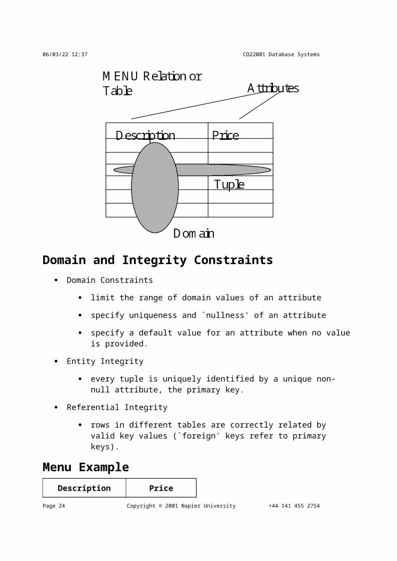
Relational Data Structure A relational data structure is a collection of tables or relations.
A relation is a collection of rows or tuples
A tuple is a collection of columns or attributes
A domain is a pool of values from which the actual attribute values are taken.
Domain and Integrity Constraints Domain Constraints
Page 18 Copyright © 2001 Napier University +44 141 455 2754

CO22001 Database Systems Student Notes
limit the range of domain values of an attribute
specify uniqueness and `nullness' of an attribute
specify a default value for an attribute when no value is provided.
Entity Integrity
every tuple is uniquely identified by a unique non-null attribute, the primary key.
Referential Integrity
rows in different tables are correctly related by valid key values (`foreign' keys refer to primary keys).
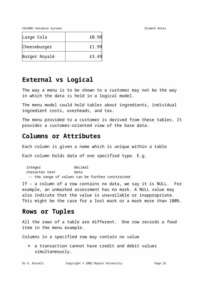
Menu Example Description Price
Large Cola £0.99
Cheeseburger £1.99
Burger Royalé £3.49
External vs Logical The way a menu is to be shown to a customer may not be the way in which the data is held in a logical model.
The menu model could hold tables about ingredients, individual ingredient costs, overheads, and tax.
The menu provided to a customer is derived from these tables. It provides a customer-oriented view of the base data.
Columns or Attributes Each column is given a name which is unique within a table
Each column holds data of one specified type. E.g.
integer decimal character text data -- the range of values can be further constrained
If – a column of a row contains no data, we say it is NULL. For example, an unmarked assessment has no mark. A NULL value may also indicate that the value is unavailable or inappropriate. This might be the case for a lost mark or a mark more than 100%.
Dr G. Russell Copyright © 2002 Napier University Page 19
School of Computing, 01/03/-1,
NULL is not a value in SQL. You can’t use the relational operators on it.

08/05/23 15:03 CO22001 Database Systems
Rows or Tuples All the rows of a table are different. One row records a food item in the menu example.
Columns in a specified row may contain no value
a transaction cannot have credit and debit values simultaneously.
Some columns must contain values for all rows
date and source, which make the row unique, in the bank account case.
Cardinality is the number of ROWS in a table.
Arity is the number of COLUMNS in a table.
Primary Keys A table requires a key which uniquely identifies each row in the table. This is entity integrity.
The key could have one column, or it could use all the columns. It should not use more columns than necessary. A key with more than one column is called a composite key.
A table may have several possible keys, the candidate keys, from which one is chosen as the primary key.
No part of a primary key may be NULL.
i If the rows of the data are not unique, it is necessary to generate an artificial primary key.
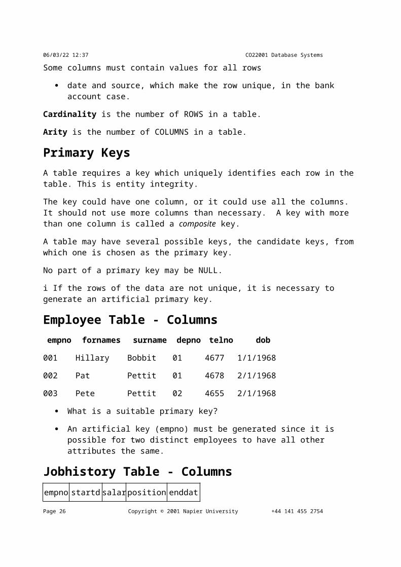
Employee Table - Columns empno fornames surname depno telno dob
001 Hillary Bobbit 01 4677 1/1/1968
002 Pat Pettit 01 4678 2/1/1968
003 Pete Pettit 02 4655 2/1/1968
What is a suitable primary key?
An artificial key (empno) must be generated since it is possible for two distinct employees to have all other attributes the same.
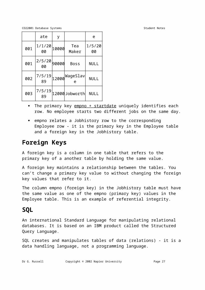
Jobhistory Table - Columns empno startdate salary position enddate
001 1/1/2000 10000 Tea Maker 1/5/2000
001 2/5/2000 90000 Boss NULLPage 20 Copyright © 2001 Napier University +44 141 455 2754
CO22001 Database Systems Student Notes
002 7/5/1989 12000 WageSlave NULL
003 7/5/1989 12000 Jobworth NULL
The primary key empno + startdate uniquely identifies each row. No employee starts two different jobs on the same day.
empno relates a Jobhistory row to the corresponding Employee row - it is the primary key in the Employee table and a foreign key in the Jobhistory table.
Foreign Keys A foreign key is a column in one table that refers to the primary key of a another table by holding the same value.
A foreign key maintains a relationship between the tables. You can’t change a primary key value to without changing the foreign key values that refer to it.
The column empno (foreign key) in the Jobhistory table must have the same value as one of the empno (primary key) values in the Employee table. This is an example of referential integrity.
SQL An international Standard Language for manipulating relational databases. It is based on an IBM product called the Structured Query Language.
SQL creates and manipulates tables of data (relations) - it is a data handling language, not a programming language.
A table is a collection of rows (tuples or records).
A row is a collection of columns (attributes).
SQL Basics Basic SQL Statements include:
CREATE - a data structure
SELECT - read one or more rows from a table
INSERT - one or more rows into a table
DELETE - one or more rows from a table
UPDATE - change the column values in a row
DROP - a data structure
Dr G. Russell Copyright © 2002 Napier University Page 21

08/05/23 15:03 CO22001 Database Systems
CREATE table employee CREATE TABLE employee ( empno INTEGER PRIMARY KEY, surname VARCHAR(15), forenames VARCHAR(30), dob date, address VARCHAR(50), telno VARCHAR(50), depno INTEGER REFERENCES department(depno), CHECK(dob IS NULL OR (dob > '1-jan-1950' AND dob < '31-dec-1980') ) );
CREATE Table Jobhistory CREATE TABLE jobhistory ( empno INTEGER REFERENCES employee(empno) position VARCHAR(30), startdate date, enddate date, salary DECIMAL(8,2), PRIMARY KEY(empno,position) );
Page 22 Copyright © 2001 Napier University +44 141 455 2754

CO22001 Database Systems Student Notes
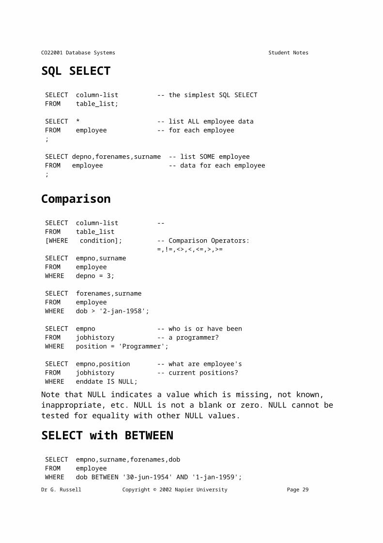
SQL SELECT SELECT column-list -- the simplest SQL SELECT FROM table_list;
SELECT * -- list ALL employee data FROM employee -- for each employee ;
SELECT depno,forenames,surname -- list SOME employee FROM employee -- data for each employee ;
Comparison SELECT column-list -- FROM table_list [WHERE condition]; -- Comparison Operators: =,!=,<>,<,<=,>,>= SELECT empno,surname FROM employee WHERE depno = 3;
SELECT forenames,surname FROM employee WHERE dob > '2-jan-1958';
SELECT empno -- who is or have been FROM jobhistory -- a programmer? WHERE position = 'Programmer';
SELECT empno,position -- what are employee's FROM jobhistory -- current positions? WHERE enddate IS NULL;
Note that NULL indicates a value which is missing, not known, inappropriate, etc. NULL is not a blank or zero. NULL cannot be tested for equality with other NULL values.
SELECT with BETWEEN SELECT empno,surname,forenames,dob FROM employee WHERE dob BETWEEN '30-jun-1954' AND '1-jan-1959';
Note that the BETWEEN predicate is inclusive. The above condition is equivalent to :
WHERE dob >= '30-jun-1954' AND <='1-jan-1959';
Dr G. Russell Copyright © 2002 Napier University Page 23

08/05/23 15:03 CO22001 Database Systems
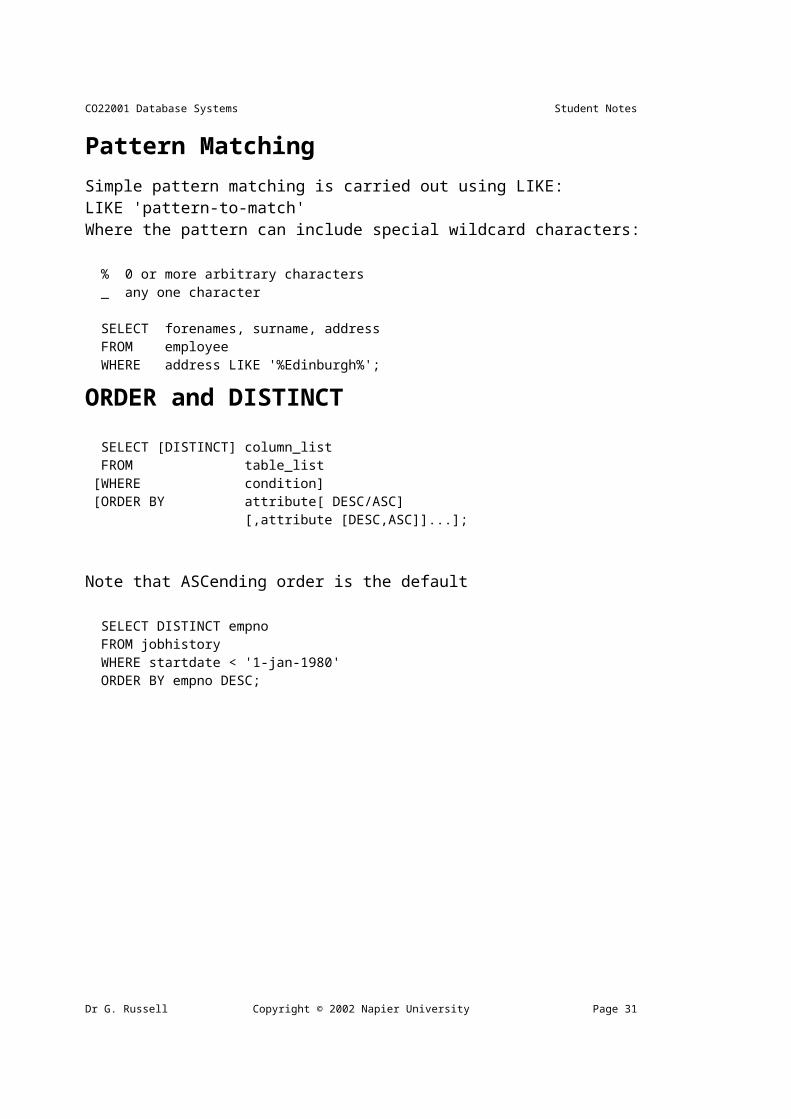
Pattern Matching Simple pattern matching is carried out using LIKE:LIKE 'pattern-to-match'Where the pattern can include special wildcard characters:
% 0 or more arbitrary characters _ any one character
SELECT forenames, surname, address FROM employee WHERE address LIKE '%Edinburgh%';
ORDER and DISTINCT SELECT [DISTINCT] column_list FROM table_list [WHERE condition] [ORDER BY attribute[ DESC/ASC] [,attribute [DESC,ASC]]...];
Note that ASCending order is the default
SELECT DISTINCT empno FROM jobhistory WHERE startdate < '1-jan-1980' ORDER BY empno DESC;
Page 24 Copyright © 2001 Napier University +44 141 455 2754
CO22001 Database Systems Student Notes
Unit 1.3 - SQL 2Unit 1.3 - Logical Operators
NOT, AND, OR (decreasing precedence),the usual operators on boolean values.
Find those who are neither accountants nor analysts who are currently paid £16,000 to £30,000:
SELECT empno FROM jobhistory WHERE salary BETWEEN 16000 AND 30000 AND enddate IS NULL AND NOT ( position LIKE '%Accountant%' OR position LIKE '%Analyst%' );
IN IN (list of values) determines whether a specified value is in a set of one or more listed
values.
List the names of employees in departments 3 or 4 born before 1950:
SELECT forenames,surname FROM employee WHERE depno IN (3,4) AND dob < '1-jan-1950';
Other SELECT capabilities SET or AGGREGATE functions
COUNT counts the rows in a table or group
SUM, AVERAGE, MIN, MAX - undertake the indicated operation on numeric columns of a table or group.
GROUP BY - forms the result of a query into groups. Set functions can then be applied to these groups.
HAVING - applies conditions to choose GROUPS of interest.
Dr G. Russell Copyright © 2002 Napier University Page 25
08/05/23 15:03 CO22001 Database Systems
Simple COUNT examples How many employees are there?
SELECT COUNT(*) FROM employee;
What is the total salary bill?
SELECT SUM(salary) totalsalary FROM jobhistory WHERE enddate IS NULL;
NOTE - the column title, `totalsalary', to be printed with the result.
Grouped COUNTs How many employees are there in each department?
SELECT depno, COUNT(depno) FROM employee GROUP BY depno;
How many employees are there in each department with more than 6 people?
SELECT depno, COUNT(depno) FROM employee GROUP BY depno HAVING COUNT(depno) > 6;
The select lists above can include only set functions and the column(s) specified in the GROUP BY clause.
Joining Tables The information required to answer a query may be spread over two or more tables
Two tables in a FROM clause are joined so that every row in one table is combined with every row in the other table. The combined table is called the Cartesian Product.
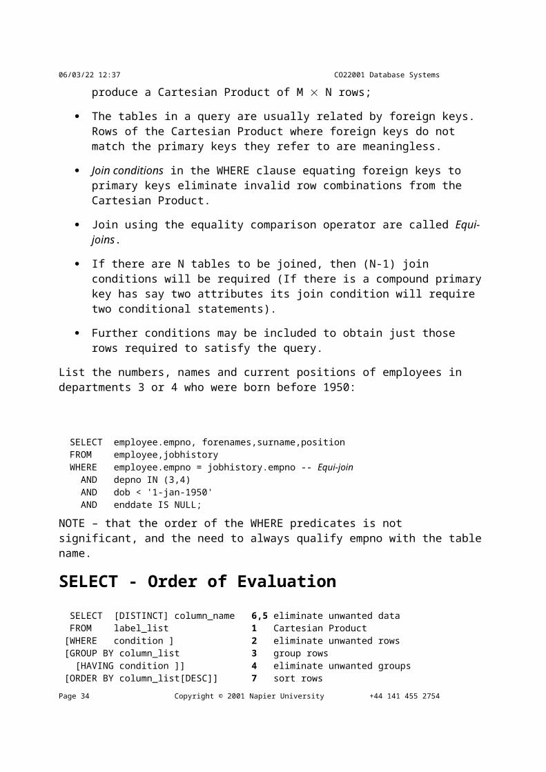
A table with M rows combined with a table of N rows will produce a Cartesian Product of M N rows;
The tables in a query are usually related by foreign keys. Rows of the Cartesian Product where foreign keys do not match the primary keys they refer to are meaningless.
Join conditions in the WHERE clause equating foreign keys to primary keys eliminate invalid row combinations from the Cartesian Product.
Join using the equality comparison operator are called Equi-joins.
If there are N tables to be joined, then (N-1) join conditions will be required (If there is a
Page 26 Copyright © 2001 Napier University +44 141 455 2754
CO22001 Database Systems Student Notes
compound primary key has say two attributes its join condition will require two conditional statements).
Further conditions may be included to obtain just those rows required to satisfy the query.
List the numbers, names and current positions of employees in departments 3 or 4 who were born before 1950:
SELECT employee.empno, forenames,surname,position FROM employee,jobhistory WHERE employee.empno = jobhistory.empno -- Equi-join AND depno IN (3,4) AND dob < '1-jan-1950' AND enddate IS NULL;
NOTE – that the order of the WHERE predicates is not significant, and the need to always qualify empno with the table name.
SELECT - Order of Evaluation SELECT [DISTINCT] column_name 6,5 eliminate unwanted data FROM label_list 1 Cartesian Product [WHERE condition ] 2 eliminate unwanted rows [GROUP BY column_list 3 group rows [HAVING condition ]] 4 eliminate unwanted groups [ORDER BY column_list[DESC]] 7 sort rows
The last four components are optional.
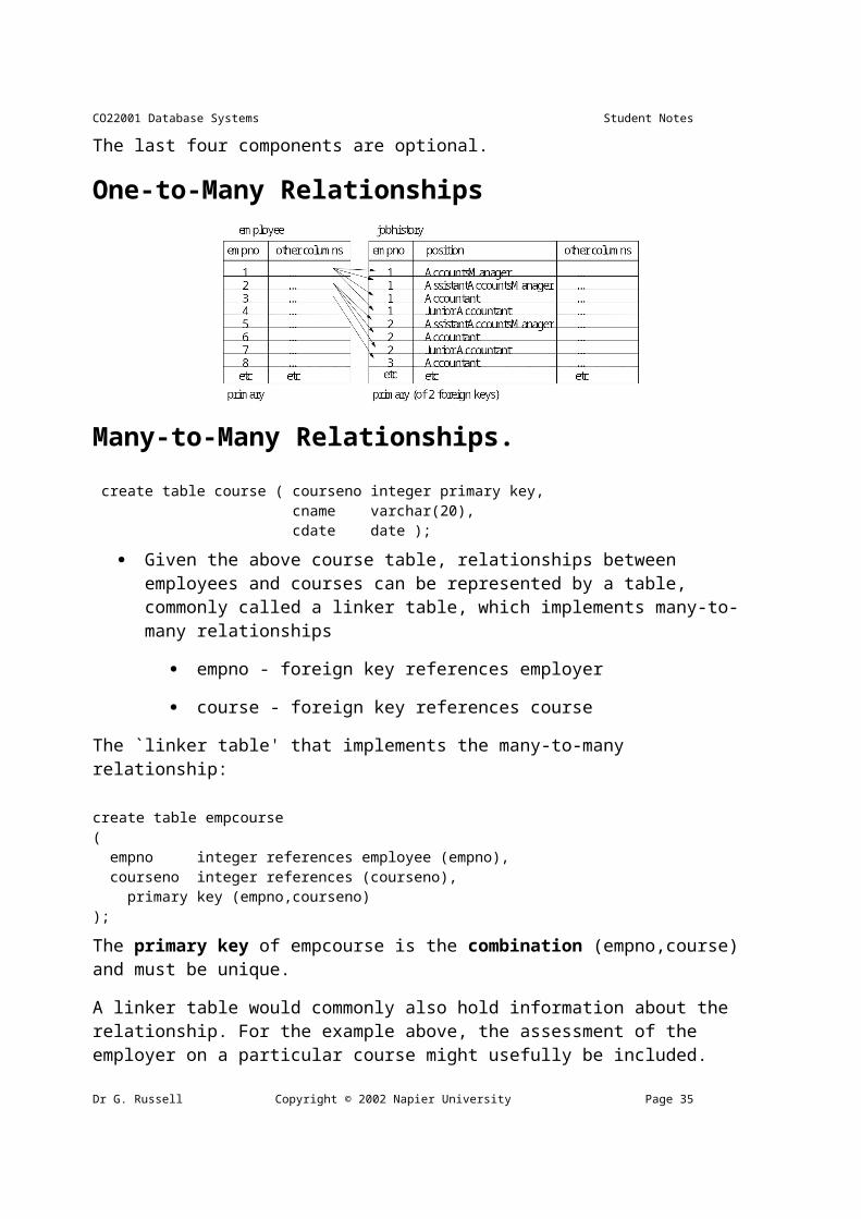
One-to-Many Relationships
Many-to-Many Relationships. create table course ( courseno integer primary key, cname varchar(20), cdate date );
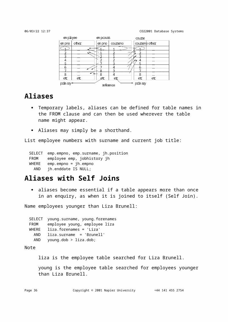
Given the above course table, relationships between employees and courses can be represented by a table, commonly called a linker table, which implements many-to-many relationships
Dr G. Russell Copyright © 2002 Napier University Page 27
School of Computing, 01/03/-1,
? Only 1 and 5 are required.
School of Computing, 01/03/-1,
DISTINCT is applied after column selection.
08/05/23 15:03 CO22001 Database Systems
empno - foreign key references employer
course - foreign key references course
The `linker table' that implements the many-to-many relationship:
create table empcourse( empno integer references employee (empno), courseno integer references (courseno), primary key (empno,courseno));
The primary key of empcourse is the combination (empno,course) and must be unique.
A linker table would commonly also hold information about the relationship. For the example above, the assessment of the employer on a particular course might usefully be included.
Aliases Temporary labels, aliases can be defined for table names in the FROM clause and can
then be used wherever the table name might appear.
Aliases may simply be a shorthand.
List employee numbers with surname and current job title:
SELECT emp.empno, emp.surname, jh.position FROM employee emp, jobhistory jh WHERE emp.empno = jh.empno AND jh.enddate IS NULL;
Aliases with Self Joins aliases become essential if a table appears more than once in an enquiry, as when it is
joined to itself (Self Join).
Name employees younger than Liza Brunell:
SELECT young.surname, young.forenames FROM employee young, employee liza
Page 28 Copyright © 2001 Napier University +44 141 455 2754

CO22001 Database Systems Student Notes
WHERE liza.forenames = 'Liza' AND liza.surname = 'Brunell' AND young.dob > liza.dob;
Note
liza is the employee table searched for Liza Brunell.
young is the employee table searched for employees younger than Liza Brunell.
Dr G. Russell Copyright © 2002 Napier University Page 29
08/05/23 15:03 CO22001 Database Systems
Unit 1.4 - SQL 3Unit 1.4 - Subqueries
One SELECT query can be used within another. It appear in the WHERE condition and is then known as a subquery
A subquery can return only one attribute having zero or more values
A subquery may provide a simpler query format than a self-join
Simple Example Name employees younger than Liza Brunell:
SELECT surname,forenames FROM employee WHERE dob < ( SELECT dob FROM employee -- subquery WHERE forenames = 'Liza' AND surname = 'Brunell');
Note - there is no need to use aliases for the employee table since the main query does not see the table used by the subquery and the subquery does not use the table employed by the main query.
Subqueries with ANY, ALL ANY or ALL can be used to qualify tests carried out on the values in the set returned by a
subquery.
List employees currently earning less than anyone now in programming:
SELECT empno FROM jobhistory WHERE salary < ALL ( SELECT salary FROM jobhistory -- subquery WHERE position LIKE '%Programmer%' AND enddate IS NULL) AND enddate IS NULL;
Subqueries with IN, NOT IN IN and NOT IN can be used to test if a value is or is not present in the set of values
returned by a subquery
List the names and employee numbers of all those who have never been on a training course:
SELECT empno,forenames,surname FROM employee
Page 30 Copyright © 2001 Napier University +44 141 455 2754

CO22001 Database Systems Student Notes
WHERE empno NOT IN (SELECT DISTINCT empno FROM empcourse);
Subqueries with EXISTS EXISTS tests if a set returned by a subquery is empty
List the employee number and job title of all those employees who do a job someone else also does:
SELECT empno FROM jobhistory mainjh WHERE enddate IS NULL AND EXISTS ( SELECT empno FROM jobhistory subjh WHERE enddate IS NULL AND mainjh.position = subjh.position AND mainjh.empno != subjh.empno );
Note that aliases are needed to enable references from subquery to main query
UNION of Subqueries A query included two or more subqueries connected by a set operation such as UNION
(MINUS or INTERSECT).
UNION returns all the distinct rows returned by two subqueries
List the number of each employee in departments 2 or 4, plus employees who know about administration:
(SELECT empno FROM employee WHERE depno IN (2,4)) UNION (SELECT empno FROM course,empcourse WHERE course.courseno = empcourse.courseno AND cname LIKE '%Administration%');
Views A view is a named query.
CREATE VIEW view_name [(column_list)] AS query;
Attributes can be renamed in column_list if required.
Suppose a user needs to regularly manipulate details about employee, name, and current position. It might be simpler to create a view limited to this information only, rather than always extracting it from two tables:
CREATE VIEW empjob ASDr G. Russell Copyright © 2002 Napier University Page 31
08/05/23 15:03 CO22001 Database Systems
SELECT employee.empno,surname,forenames,position FROM employee,jobhistory WHERE employee.empno = jobhistory.empno AND enddate IS NULL;
A view can be accessed like any other table
List those currently in Programming type jobs:
SELECT empno,surname,forenames FROM empjob WHERE position LIKE '%Program%';
A view can (should) be dropped when no longer required:
DROP VIEW view_name
The use of a view may provide a simpler query format than using self-joins or subqueries
Name employees younger than Liza Brunell:
CREATE VIEW liza AS SELECT dob FROM employee WHERE forenames = 'Liza' AND surname = 'Brunell'; SELECT surname,forenames FROM employee,liza WHERE employee.dob > liza.dob; DROP VIEW liza;
View Manipulation When is a view `materialised' or populated with rows of data?
When it is defined or
when it is accessed
If it is the former then subsequent inserts, deletes and updates would not be visible. If the latter then changes will be seen.
Some systems allow you to chose when views are materialised, most do not and views are materialised whenever they are accessed thus all changes can be seen.
VIEW update, insert and delete Can we change views?
Yes, provided the primary key of all the base tables which make up the view are present in the view.
Page 32 Copyright © 2001 Napier University +44 141 455 2754

CO22001 Database Systems Student Notes
Base Table - A Base Table - BA# B#
View Definition
A# B#View
This view cannot be changed because we have no means of knowing which row of B to modify
Base Table - A Base Table - BA# B#
View Definition
A#View
Other SQL Statements So far we have just looked at SELECT but we need to be able to do other operations as
follows:
INSERT - which writes new rows into a database
DELETE - which deletes rows from a database
UPDATE - which changes values in existing rows
We also need to be able to control access to out tables by other users (see the later SECURITY lecture).
We may need to provide special views of tables to make queries easier to write. These Dr G. Russell Copyright © 2002 Napier University Page 33

08/05/23 15:03 CO22001 Database Systems
views can also be made available to other users so that they can easily see our data but not change it in any way.
INSERT INSERT INTO table_name [(column_list)] VALUES (value_list)
The column_list lists columns to be assigned values. It can be omitted if every column is to be assigned a value. The value_list is a set of literal values giving the value for each column in column_list or CREATE TABLE order.
insert into course values (11,'Advanced Accounting',10-jan-2000); insert into course (courseno,cname) values(13,'Advanced Administration');
DELETE DELETE FROM table_name [WHERE condition];
the rows of table_name which satify the condition are deleted.
Delete Examples:
DELETE FROM jobhistory -- remote current posts from jobhistoryWHERE enddate IS NULL;
DELETE FROM jobhistory -- Remove all posts from jobhistory,; -- leaving an empty table
DROP table jobhistory; -- Remove jobhistory table completely
UPDATE UPDATE table_name SET column_name = expression,{column_name=expression} [WHERE condition]
The expression can be
NULL
a literal value
an expression based upon the current column value
Give a salary rise of 10% to all accountants:
UPDATE jobhistory SET salary = salary * 1.10 WHERE position LIKE '%Accountant%' AND enddate IS NULL;
Page 34 Copyright © 2001 Napier University +44 141 455 2754
CO22001 Database Systems Student Notes
Unit 2.1 - Data AnalysisUnit 2.1: Database AnalysisThis unit it concerned with the process of taking a database specification from a customer and implementing the underlying database structure necessary to support that specification.
Entity Relationship ModellingData analysis is concerned with the NATURE and USE of data. It involves the identification of the data elements which are needed to support the data processing system of the organization, the placing of these elements into logical groups and the definition of the relationships between the resulting groups.
Other approaches, e.g. D.F.Ds and Flowcharts, have been concerned with the flow of data dataflow methodologies. Data analysis is one of several data structure based methodologies Jackson SP/D is another.
Systems analysts often, in practice, go directly from fact finding to implementation dependent data analysis. Their assumptions about the usage of properties of and relationships between data elements are embodied directly in record and file designs and computer procedure specifications. The introduction of Database Management Systems (DBMS) has encouraged a higher level of analysis, where the data elements are defined by a logical model or `schema' (conceptual schema). When discussing the schema in the context of a DBMS, the effects of alternative designs on the efficiency or ease of implementation is considered, i.e. the analysis is still somewhat implementation dependent. If we consider the data relationships, usages and properties that are important to the business without regard to their representation in a particular computerised system using particular software, we have what we are concerned with, implementationindependent data analysis.
It is fair to ask why data analysis should be done if it is possible, in practice to go straight to a computerised system design. Data analysis is time consuming; it throws up a lot of questions. Implementation may be slowed down while the answers are sought. It is more expedient to have an experienced analyst `get on with the job' and come up with a design straight away. The main difference is that data analysis is more likely to result in a design which meets both present and future requirements, being more easily adapted to changes in the business or in the computing equipment. It can also be argued that it tends to ensure that policy questions concerning the organisations' data are answered by the managers of the organisation, not by the systems analysts. Data analysis may be thought of as the `slow and careful' approach, whereas omitting this step is `quick and dirty'.
From another viewpoint, data analysis provides useful insights for general design principals which will benefit the trainee analyst even if he finally settles for a `quick and dirty' solution.
The development of techniques of data analysis have helped to understand the structure and meaning of data in organisations. Data analysis techniques can be used as the first step of extrapolating the complexities of the real world into a model that can be held on a computer and
Dr G. Russell Copyright © 2002 Napier University Page 35
08/05/23 15:03 CO22001 Database Systems
be accessed by many users. The data can be gathered by conventional methods such as interviewing people in the organisation and studying documents. The facts can be represented as objects of interest. There are a number of documentation tools available for data analysis, such as entityrelationship diagrams. These are useful aids to communication, help to ensure that the work is carried out in a thorough manner, and ease the mapping processes that follow data analysis. Some of the documents can be used as source documents for the data dictionary.
In data analysis we analyse the data and build a systems representation in the form of a data model (conceptual). A conceptual data model specifies the structure of the data and the processes which use that data.
Data Analysis = establishing the nature of data.
Functional Analysis = establishing the use of data.
However, since Data and Functional Analysis are so intermixed, we shall use the term Data Analysis to cover both.
Building a model of an organisation is not easy. The whole organisation is too large as there will be too many things to be modelled. It takes too long and does not achieve anything concrete like an information system, and managers want tangible results fairly quickly. It is therefore the task of the data analyst to model a particular view of the organisation, one which proves reasonable and accurate for most applications and uses. Data has an intrinsic structure of its own, independent of processing, reports formats etc. The data model seeks to make explicit that structure
Data analysis was described as establishing the nature and use of data.
Database Analysis Life Cycle
Database study
Testing and evaluation
maintenance and evolution
Database design
Operation
Implementation and loading
When a database designer is approaching the problem of constructing a database system, the logical steps followed is that of the database analysis life cycle:
Database study - here the designer creates a written specification in words for the database system to be built. This involves
Page 36 Copyright © 2001 Napier University +44 141 455 2754
CO22001 Database Systems Student Notes
analysing the company situation - is it an expanding company, dynamic in its requirements, mature in nature, solid background in employee training for new internal products, etc. These have an impact on how the specification is to be viewed.
define problems and constraints - what is the situation currently? How does the company deal with the task which the new database is to perform. Any issues around the current method? What are the limits of the new system?
define objectives - what is the new database system going to have to do, and in what way must it be done. What information does the company want to store specifically, and what does it want to calculate. How will the data evolve.
define scope and boundaries - what is stored on this new database system, and what it stored elsewhere. Will it interface to another database?
Database Design - conceptual, logical, and physical design steps in taking specifications to physical implementable designs. This is looked at more closely in a moment.
Implementation and loading - it is quite possible that the database is to run on a machine which as yet does not have a database management system running on it at the moment. If this is the case one must be installed on that machine. Once a DBMS has been installed, the database itself must be created within the DBMS. Finally, not all databases start completely empty, and thus must be loaded with the initial data set (such as the current inventory, current staff names, current customer details, etc).
Testing and evaluation - the database, once implemented, must be tested against the specification supplied by the client. It is also useful to test the database with the client using mock data, as clients do not always have a full understanding of what they thing they have specified and how it differs from what they have actually asked for! In addition, this step in the life cycle offers the chance to the designer to fine-tune the system for best performance. Finally, it is a good idea to evaluate the database in-situ, along with any linked applications.
Operation - this step is where the system is actually in real usage by the company.
Maintenance and evolution - designers rarely get everything perfect first time, and it may be the case that the company requests changes to fix problems with the system or to recommend enhancements or new requirements.
Commonly development takes place without change to the database structure. In elderly systems the DB structure becomes fossilised.
Three-level Database Model
Often referred to as the three-level model, this is where the design moves from a written specification taken from the real-world requirements to a physically-implementable design for a specific DBMS. The three levels commonly referred to are `Conceptual Design', `Data Model Mapping', and `Physical Design'.
Dr G. Russell Copyright © 2002 Napier University Page 37

08/05/23 15:03 CO22001 Database Systems
The specification is usually in the form of a written document containing customer requirements, mock reports, screen drawings and the like, written by the client to indicate the requirements which the final system is to have. Often such data has to be collected together from a variety of internal sources to the company and then analysed to see if the requirements are necessary, correct, and efficient.
Once the Database requirements have been collated, the Conceptual Design phase takes the requirements and produces a high-level data model of the database structure. In this module, we use ER modelling to represent high-level data models, but there are other techniques. This model is independent of the final DBMS which the database will be installed in.
Next, the Conceptual Design phase takes the high-level data model it taken and converted into a conceptual schema, which is specific to a particular DBMS class (e.g. relational). For a relational system, such as Oracle, an appropriate conceptual schema would be relations.
Finally, in the Physical Design phase the conceptual schema is converted into database internal structures. This is specific to a particular DBMS product.
Entity Relationship Modelling Entity Relationship (ER) modelling
is a design tool
is a graphical representation of the database system
provides a high-level conceptual data model
supports the user's perception of the data
is DBMS and hardware independent
had many variants
is composed of entities, attributes, and relationships
Page 38 Copyright © 2001 Napier University +44 141 455 2754
CO22001 Database Systems Student Notes
Entities An entity is any object in the system that we want to model and store information about
Individual objects are called entities
Groups of the same type of objects are called entity types or entity sets
Entities are represented by rectangles (either with round or square corners)
Lecturer Lecturer
Chen's notation other notations There are two types of entities; weak and strong entity types.
Attribute All the data relating to an entity is held in its attributes.
An attribute is a property of an entity.
Each attribute can have any value from its domain.
Each entity within an entity type:
May have any number of attributes.
Can have different attribute values than that in any other entity.
Have the same number of attributes.
Attributes can be
simple or composite
single-valued or multi-valued
Attributes can be shown on ER models
They appear inside ovals and are attached to their entity.
Note that entity types can have a large number of attributes... If all are shown then the diagrams would be confusing. Only show an attribute if it adds information to the ER diagram, or clarifies a point.
Dr G. Russell Copyright © 2002 Napier University Page 39

08/05/23 15:03 CO22001 Database Systems
LecturerName
Keys A key is a data item that allows us to uniquely identify individual occurrences or an
entity type.
A candidate key is an attribute or set of attributes that uniquely identifies individual occurrences or an entity type.
An entity type may have one or more possible candidate keys, the one which is selected is known as the primary key.
A composite key is a candidate key that consists of two or more attributes
The name of each primary key attribute is underlined.
Relationships A relationship type is a meaningful association between entity types
A relationship is an association of entities where the association includes one entity from each participating entity type.
Relationship types are represented on the ER diagram by a series of lines.
As always, there are many notations in use today...
In the original Chen notation, the relationship is placed inside a diamond, e.g. managers manage employees:
Manager manages Employee
For this module, we will use an alternative notation, where the relationship is a label on the line. The meaning is identical
Manager Employeemanages
Degree of a Relationship The number of participating entities in a relationship is known as the degree of the
relationship.
If there are two entity types involved it is a binary relationship type
Page 40 Copyright © 2001 Napier University +44 141 455 2754

CO22001 Database Systems Student Notes
Manager Employeemanages
If there are three entity types involved it is a ternary relationship type
Customer
SalesAssistant
sells Product
It is possible to have a n-ary relationship (e.g. quaternary or unary).
Unary relationships are also known as a recursive relationship.
Employee
manages
It is a relationship where the same entity participates more than once in different roles.
In the example above we are saying that employees are managed by employees.
If we wanted more information about who manages whom, we could introduce a second entity type called manager.
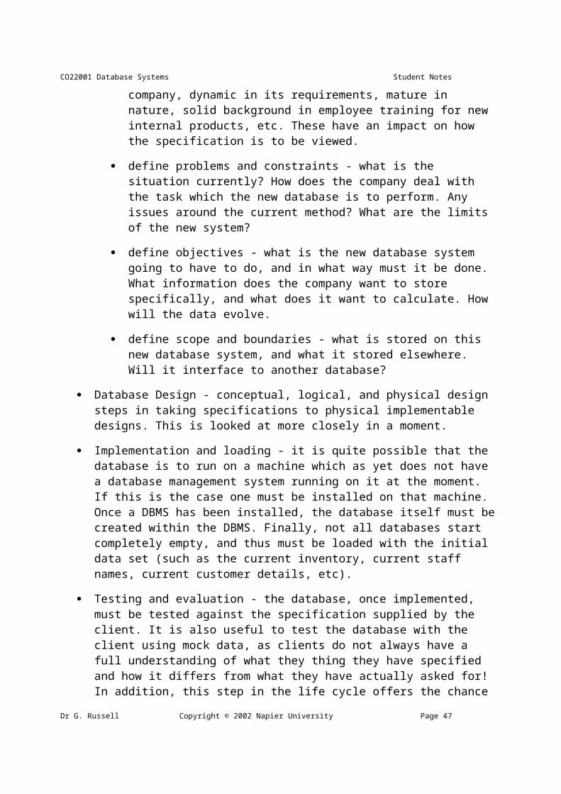
Degree of a Relationship It is also possible to have entities associated through two or more distinct relationships.
EmployeeDepartmentmanages
employs
In the representation we use it is not possible to have attributes as part of a relationship. To support this other entity types need to be developed.
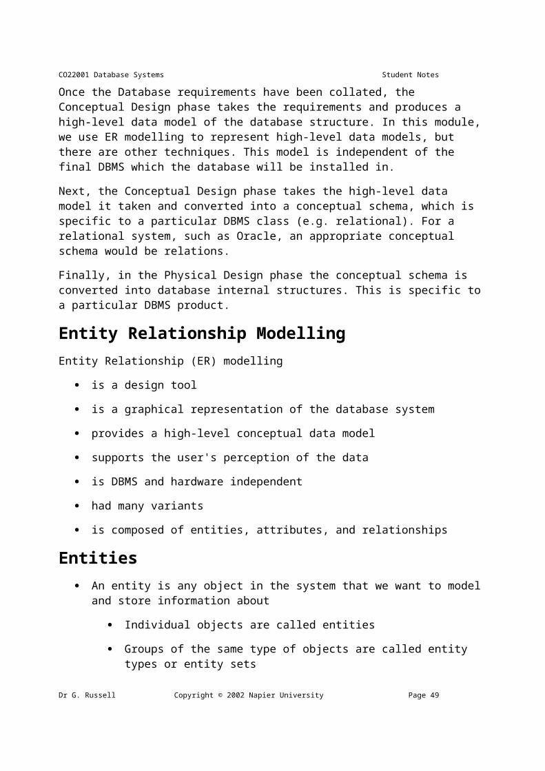
Replacing ternary relationships When ternary relationships occurs in an ER model they should always be removed before finishing the model. Sometimes the relationships can be replaced by a series of binary relationships that link pairs of the original ternary relationship.
Dr G. Russell Copyright © 2002 Napier University Page 41

08/05/23 15:03 CO22001 Database Systems
Customer
SalesAssistant
sells Product
assists buys
This can result in the loss of some information - It is no longer clear which sales assistant sold a customer a particular product.
Try replacing the ternary relationship with an entity type and a set of binary relationships.
Relationships are usually verbs, so name the new entity type by the relationship verb rewritten as a noun.
The relationship sells can become the entity type sale.
SalesAssistant
Customer
Sale Productinvolvesmakes
requests
So a sales assistant can be linked to a specific customer and both of them to the sale of a particular product.
This process also works for higher order relationships.
Cardinality Relationships are rarely one-to-one
For example, a manager usually manages more than one employee
This is described by the cardinality of the relationship, for which there are four possible categories.
One to one (1:1) relationship
One to many (1:m) relationship
Many to one (m:1) relationship
Many to many (m:n) relationship
On an ER diagram, if the end of a relationship is straight, it represents 1, while a "crow's foot" end represents many.
A one to one relationship - a man can only marry one woman, and a woman can only marry one man, so it is a one to one (1:1) relationship
Man Woman1 is married to 1
Page 42 Copyright © 2001 Napier University +44 141 455 2754

CO22001 Database Systems Student Notes
A one to may relationship - one manager manages many employees, but each employee only has one manager, so it is a one to many (1:n) relationship
Manager Employeemanages m1
A many to one relationship - many students study one course. They do not study more than one course, so it is a many to one (m:1) relationship
Student Coursestudies 1m
A many to many relationship - One lecturer teaches many students and a student is taught by many lecturers, so it is a many to many (m:n) relationship
Lecturer Studentteachesm n
Optionality A relationship can be option or mandatory.
If the relationship is mandatory
an entity at one end of the relationship must be related to an entity at the other end.
The optionality can be different at each end of the relationship
For example, a student must be on a course. This is mandatory. To the relationship `student studies course' is mandatory.
But a course can exist before any students have enrolled. Thus the relationship `course is_studied_by student' is optional.
To show optionality, put a circle or `0' at the `optional end' of the relationship.
As the optional relationship is `course is_studied_by student', and the optional part of this is the student, then the `O' goes at the student end of the relationship connection.
Course Studentis studied by0
It is important to know the optionality because you must ensure that whenever you create a new entity it has the required mandatory links.
Entity Sets Sometimes it is useful to try out various examples of entities from an ER model. One reason for this is to confirm the correct cardinality and optionality of a relationship. We use an `entity set
Dr G. Russell Copyright © 2002 Napier University Page 43

08/05/23 15:03 CO22001 Database Systems
diagram' to show entity examples graphically. Consider the example of `course is_studied_by student'.
BSc CompMSc Biology
BA Fine ArtBSc Maths
SarahAndyJim
Anne
PaulJenny
Examples of the"Student" entities
Examples of the"Course" entities
the "is_studied_by"relationship
Confirming Correctness
BSc Comp
MSc Biology
BA Fine ArtBSc Maths
SarahAndyJim
Anne
PaulJenny
Examples of the"Student" entities
Examples of the"Course" entities
the "is_studied_by"relationship
Use the diagram to show all possible relationship scenarios.
Go back to the requirements specification and check to see if they are allowed.
If not, then put a cross through the forbidden relationships
This allows you to show the cardinality and optionality of the relationship
Deriving the relationship parameters To check we have the correct parameters (sometimes also known as the degree) of a relationship, ask two questions:
One course is studied by how many students? Answer = `zero or more'.
This gives us the degree at the `student' end.
The answer `zero or more' needs to be split into two parts.
The `more' part means that the cardinality is `many'.
The `zero' part means that the relationship is `optional'.
If the answer was `one or more', then the relationship would be `mandatory'.
2. One student studies how many courses? Answer = `One' Page 44 Copyright © 2001 Napier University +44 141 455 2754
CO22001 Database Systems Student Notes
This gives us the degree at the `course' end of the relationship.
The answer `one' means that the cardinality of this relationship is 1, and is `mandatory'
If the answer had been `zero or one', then the cardinality of the relationship would have been 1, and be `optional'.
Redundant relationships Some ER diagrams end up with a relationship loop.
check to see if it is possible to break the loop without losing info
Given three entities A, B, C, where there are relations A-B, B-C, and C-A, check if it is possible to navigate between A and C via B. If it is possible, then A-C was a redundant relationship.
Always check carefully for ways to simplify your ER diagram. It makes it easier to read the remaining information.
Redundant relationships example Consider entities `customer' (customer details), `address' (the address of a customer) and
`distance' (distance from the company to the customer address).
Customer
Distance
Address
far from workfar from work
is living at
Splitting n:m Relationships A many to many relationship in an ER model is not necessarily incorrect. They can be replaced using an intermediate entity. This should only be done where:
the m:n relationship hides an entity
the resulting ER diagram is easier to understand.
Splitting n:m Relationships - Example Consider the case of a car hire company. Customers hire cars, one customer hires many card and a car is hired by many customers.
m nhire CarCustomer
The many to many relationship can be broken down to reveal a `hire' entity, which contains an
Dr G. Russell Copyright © 2002 Napier University Page 45

08/05/23 15:03 CO22001 Database Systems
attribute `date of hire'.
CarCustomerm n
Hire
Constructing an ER model - Entities Before beginning to draw the ER model, read the requirements specification carefully. Document any assumptions you need to make.
1. Identify entities - list all potential entity types. These are the object of interest in the system. It is better to put too many entities in at this stage and them discard them later if necessary.
2. Remove duplicate entities - Ensure that they really separate entity types or just two names for the same thing.
Also do not include the system as an entity type
e.g. if modelling a library, the entity types might be books, borrowers, etc.
The library is the system, thus should not be an entity type.
Constructing an ER model - Attributes 3. List the attributes of each entity (all properties to describe the entity which are relevant to
the application).
Ensure that the entity types are really needed.
are any of them just attributes of another entity type?
if so keep them as attributes and cross them off the entity list.
Do not have attributes of one entity as attributes of another entity!
4. Mark the primary keys.
Which attributes uniquely identify instances of that entity type?
This may not be possible for some weak entities.
Constructing an ER model - Relationships 5. Define the relationships
Examine each entity type to see its relationship to the others.
6. Describe the cardinality and optionality of the relationships
Examine the constraints between participating entities.
Page 46 Copyright © 2001 Napier University +44 141 455 2754

CO22001 Database Systems Student Notes
7. Remove redundant relationships
Examine the ER model for redundant relationships.
ER modelling is an iterative process, so draw several versions, refining each one until you are happy with it. Note that there is no one right answer to the problem, but some solutions are better than others!
Dr G. Russell Copyright © 2002 Napier University Page 47
08/05/23 15:03 CO22001 Database Systems
Unit 2.2 - ER Modelling 2Unit 2.2 - Entity Relationship Modelling - 2 Overview
construct an ER model
understand the problems associated with ER models
understand the modelling concepts of Enhanced ER modelling
Country Bus Company A Country Bus Company owns a number of busses. Each bus is allocated to a particular route, although some routes may have several busses. Each route passes through a number of towns. One or more drivers are allocated to each stage of a route, which corresponds to a journey through some or all of the towns on a route. Some of the towns have a garage where busses are kept and each of the busses are identified by the registration number and can carry different numbers of passengers, since the vehicles vary in size and can be single or double-decked. Each route is identified by a route number and information is available on the average number of passengers carried per day for each route. Drivers have an employee number, name, address, and sometimes a telephone number.
Entities Bus - Company owns busses and will hold information about them.
Route - Buses travel on routes and will need described.
Town - Buses pass through towns and need to know about them
Driver - Company employs drivers, personnel will hold their data.
Stage - Routes are made up of stages
Garage - Garage houses buses, and need to know where they are.
Relationships A bus is allocated to a route and a route may have several buses.
Bus-route (m:1) is serviced by
A route comprises of one or more stages.
route-stage (1:m) comprises
One or more drivers are allocated to each stage.
Page 48 Copyright © 2001 Napier University +44 141 455 2754

CO22001 Database Systems Student Notes
driver-stage (m:1) is allocated
A stage passes through some or all of the towns on a route.
stage-town (m:n) passes-through
A route passes through some or all of the towns
route-town (m:n) passes-through
Some of the towns have a garage
garage-town (1:1) is situated
A garage keeps buses and each bus has one `home' garage
garage-bus (m:1) is garaged
Draw E-R Diagram
is serviced byRouteBus
Town
GarageStage
Driveris allocated
mn
m
m
nn
has
passed throughis situated in
is garaged
Attributes Bus (reg-no,make,size,deck,no-pass)
Route (route-no,avg-pass)
Driver (emp-no,name,address,tel-no)
Town (name)
Stage (stage-no)
Garage (name,address)
Dr G. Russell Copyright © 2002 Napier University Page 49
08/05/23 15:03 CO22001 Database Systems
Problems with ER Models There are several problems that may arise when designing a conceptual data model. These are known as connection traps.
Page 50 Copyright © 2001 Napier University +44 141 455 2754

CO22001 Database Systems Student Notes
There are two main types of connection traps:
1. fan traps
2. chasm traps
Fan traps A fan trap occurs when a model represents a relationship between entity types, but the pathway between certain entity occurrences is ambiguous. It occurs when 1:m relationships fan out from a single entity.
Departmentis on
Site employ Staffmn
A single site contains many departments and employs many staff. However, which staff work in a particular department?
The fan trap is resolved by restructuring the original ER model to represent the correct association.
nSiteDepartmentStaff
m
works for is on
Chasm traps A chasm trap occurs when a model suggests the existence of a relationship between entity types, but the pathway does not exist between certain entity occurrences.
It occurs where there is a relationship with partial participation, which forms part of the pathway between entities that are related.
Branch Staffoversees
Propertyis_allocated
n 00
A single branch is allocated many staff who oversee the management of properties for rent. Not all staff oversee property and not all property is managed by a member of staff.
What properties are available at a branch?
The partial participation of Staff and Property in the oversees relation means that some properties cannot be associated with a branch office through a member of staff.
We need to add the missing relationship which is called `has' between the Branch and the Property entities.
You need to therefore be careful when you remove relationships which you consider to be redundant.
Dr G. Russell Copyright © 2002 Napier University Page 51

08/05/23 15:03 CO22001 Database Systems
Branch
Staff
Property
is_allocated oversees
has
00n
Enhanced ER Models (EER) The basic concepts of ER modelling is not powerful enough for some complex applications... We require some additional semantic modelling concepts:
Specialisation
Generalisation
Categorisation
Aggregation
First we need some new entity constructs.
Superclass - an entity type that includes distinct subclasses that require to be represented in a data model.
Subclass - an entity type that has a distinct role and is also a member of a superclass.
Staff
Manager Secretary
SalesPersonnel
Subclasses need not be mutually exclusive; a member of staff may be a manager and a sales person.
The purpose of introducing superclasses and subclasses is to avoid describing types of staff with possibly different attributes within a single entity. This could waste space and you might want to make some attributes mandatory for some types of staff but other staff would not need these attributes at all.
Specialisation This is the process of maximising the differences between members of an entity by identifying their distinguishing characteristics.
Staff(staff_no,name,address,dob)
Page 52 Copyright © 2001 Napier University +44 141 455 2754

CO22001 Database Systems Student Notes
Manager(bonus)
Secretary(wp_skills)
Sales_personnel(sales_area, car_allowance)
Staff
Manager Secretary
SalesPersonnel
Department
works for
manages
Here we have shown that the manages relationship is only applicable to the Manager subclass, whereas the works_for relationship is applicable to all staff.
It is possible to have subclasses of subclasses.
Generalisation Generalisation is the process of minimising the differences between entities by identifying common features.
This is the identification of a generalised superclass from the original subclasses. This is the process of identifying the common attributes and relationships.
Unit 2.3 - Mapping ER Models into RelationsUnit 2.3 - Mapping ER Models into Relations Overview
map 1:1 relationships into relations
map 1:m relationships into relations
map m:n relationships into relations
differences between mapping optional and mandatory relationships.
What is a relation? A relation is a table that holds the data we are interested in. It is two-dimensional and has rows and columns.
Each entity type in the ER model is mapped into a relation.
The attributes become the columns.
Dr G. Russell Copyright © 2002 Napier University Page 53
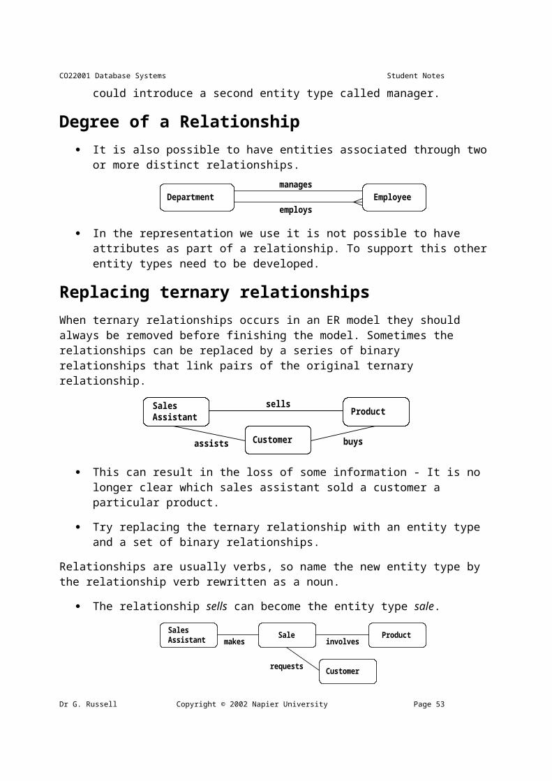
08/05/23 15:04 CO22001 Database Systems
The individual entities become the rows.
Student
name
address
matric_no
DoB
name address matric_no DoBJohn Smith Scotland
JapanPaul James0987654 12/12/991234567 1/2/33
Relations can be represented textually as:
tablename(primary key, attribute 1, attribute 2, ... , foreign key)
If matric_no was the primary key, and there were no foreign keys, then the table above could be represented as:
student(matric no, name, address, date_of_birth)
When referring to relations or tables, cardinality is considered to the the number of rows in the relation or table, and arity is the number of columns in a table or attributes in a relation.
Foreign keys A foreign key is an attribute (or group of attributes) that is the primary key to another relation.
Roughly, each foreign key represents a relationship between two entity types.
They are added to relations as we go through the mapping process.
They allow the relations to be linked together.
A relation can have several foreign keys.
It will generally have a foreign key from each table that it is related to.
Foreign keys are usually shown in italics or with a wiggly underline.
Preparing to map the ER model Before we start the actual mapping process we need to be certain that we have simplified the ER model as much as possible.
This is the ideal time to check the model, as it is really the last chance to make changes to the ER model without causing major complications.
Page 54 Copyright © 2001 Napier University +44 141 455 2754
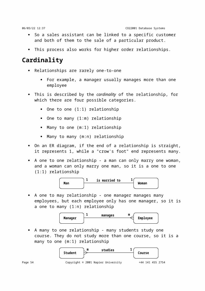
CO22001 Database Systems Student Notes
Mapping 1:1 relationships Before tackling a 1:1 relationship, we need to know its optionality.
There are three possibilities the relationship can be:
1. mandatory at both ends
2. mandatory at one end and optional at the other
3. optional at both ends
Mandatory at both ends If the relationship is mandatory at both ends it is often possible to subsume one entity type into the other.
The choice of which entity type subsumes the other depends on which is the most important entity type (more attributes, better key, semantic nature of them).
The result of this amalgamation is that all the attributes of the `swallowed up' entity become attributes of the more important entity.
The key of the subsumed entity type becomes a normal attribute.
If there are any attributes in common, the duplicates are removed.
The primary key of the new combined entity is usually the same as that of the original more important entity type.
When not to combine There are a few reason why you might not combine a 1:1 mandatory relationship.
the two entity types represent different entities in the `real world'.
the entities participate in very different relationships with other entities.
efficiency considerations when fast responses are required or different patterns of updating occur to the two different entity types.
If not combined... If the two entity types are kept separate then the association between them must be represented by a foreign key.
The primary key of one entity type comes the foreign key in the other.
It does not matter which way around it id done but you should not have a foreign key in each entity.
Dr G. Russell Copyright © 2002 Napier University Page 55
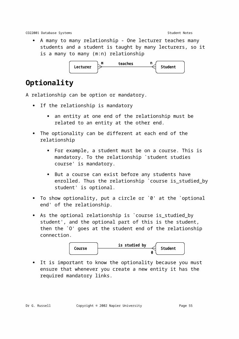
08/05/23 15:04 CO22001 Database Systems
Example Two entity types; staff and contract.
Each member of staff must have one contract and each contract must have one member of staff associated with it.
It is therefore a mandatory relations at both ends.
Staff Contract
emp_no
namehas
start end
position
salary
cont_no
These to entity types could be amalgamated into one.
Staff(emp_no, name, cont_no, start, end, position, salary)
or kept apart and a foreign key used
Staff(emp_no, name, contract_no) Contract(cont_no, start, end, position, salary)
or
Staff(emp_no, name) Contract(cont_no, start, end, position, salary, emp_no)
Mandatory Optional The entity type of the optional end may be subsumed into the mandatory end as in the previous example.
It is better NOT to subsume the mandatory end into the optional end as this will create null entries.
Staff Contract
emp_no
namehas
start end
position
salary
cont_no
0
If we add to the specification that each staff member may have at most one contract (thus making the relation optional at one end).
Map the foreign key into Staff - the key is null for staff without a contract.
Staff(emp_no, name, contract_no) Contract(cont_no, start, end, position, salary)
Map the foreign key into Contract - emp_no is mandatory thus never null.
Page 56 Copyright © 2001 Napier University +44 141 455 2754
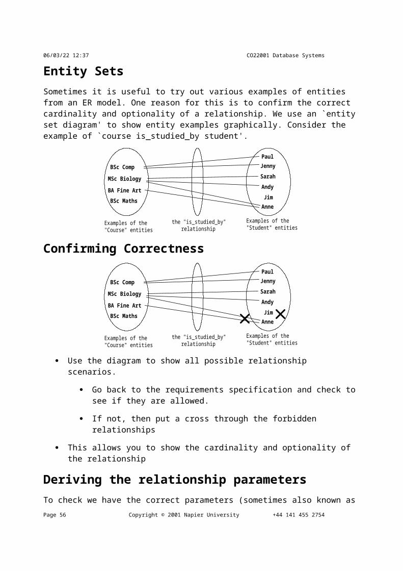
CO22001 Database Systems Student Notes
Staff(emp_no, name) Contract(cont_no, start, end, position, salary, emp_no)
Example
Consider this example: Staff “Gordon”, empno 10, contract no 11. Staff “Andrew”, empno 11, no contract. Contract 11, from 1st Jan 2001 to 10th Jan 2001, lecturer, on £2.00 a year.
Foreign key in Staff:
Contract Table:Cont_no Start End Position Salary11 1st Jan 2001 10th Jan 2001 Lecturer £2.00
Staff Table:Empno Name Contract No10 Gordon 1111 Andrew NULL
However, Foreign key in Contract:
Contract Table:Cont_no Start End Position Salary Empno11 1st Jan 2001 10th Jan 2001 Lecturer £2.00 10
Staff Table:Empno Name10 Gordon11 Andrew
As you can see, both ways store the same information, but the second way has no NULLs.
Mandatory Optional - Subsume? The reasons for not subsuming are the same as before with the following additional reason.
very few of the entities from the mandatory end are involved in the relationship. This could cause a lot of wasted space with many blank or null entries.
Dr G. Russell Copyright © 2002 Napier University Page 57
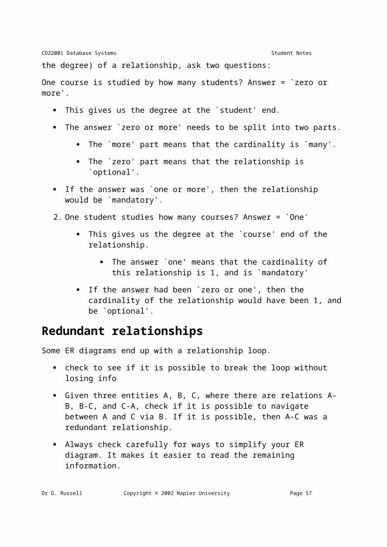
08/05/23 15:04 CO22001 Database Systems
0
lect no
l nameLecturer manages
Course
cno cname type
yr_vetted
enternal
If only a few lecturers manage courses and Course is subsumed into Lecturer then there would be many null entries in the table.
Lecturer(lect_no, l_name, cno, c_name, type, yr_vetted, external)
It would be better to keep them separate.
Lecturer(lect_no, l_name) Course(cno, c_name, type, yr_vetted, external,lect_no)
Summary... So for 1:1 optional relationships, take the primary key from the `mandatory end' and add it to the `optional end' as a foreign key.
So, given entity types A and B, where A B is a relationship where the A end it optional, the result would be:
A (primary key,attribute,...,foreign key to B) B (primary key,attribute,...)
Optional at both ends... Such examples cannot be amalgamated as you could not select a primary key. Instead, one foreign key is used as before.
0
emp_no
nameStaff leases Car
reg_no year make
type
colour0
Each staff member may lease up to one car
Each car may be leased by at most one member of staff
If these were combined together...
Staff_car(emp_no, name, reg_no, year, make, type, colour)
what would be the primary key?
If emp_no is used then all the cars which are not being leased will not have a key.
Similarly, if the reg_no is used, all the staff not leasing a car will not have a key.
Page 58 Copyright © 2001 Napier University +44 141 455 2754
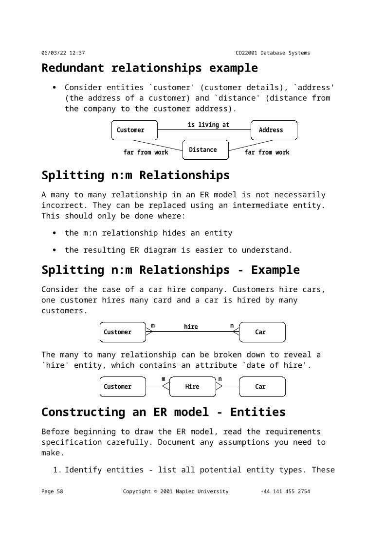
CO22001 Database Systems Student Notes
A compound key will not work either.
Mapping 1:m relationships To map 1:m relationships, the primary key on the `one side' of the relationship is added to the `many side' as a foreign key.
For example, the 1:m relationship `course-student':
Coursematriculate
Student
Assuming that the entity types have the following attributes:
Course(course_no, c_name) Student(matric_no, st_name, dob)
Then after mapping, the following relations are produced:
Course(course_no, c_name) Student(matric_no, st_name, dob, course_no)
If an entity type participates in several 1:m relationships, then you apply the rule to each relationship, and add foreign keys as appropriate.
Mapping n:m relationships If you have some m:n relationships in your ER model then these are mapped in the following manner.
A new relation is produced which contains the primary keys from both sides of the relationship
These primary keys form a composite primary key.
Studentstudies on
Module
Thus
Student(matric_no, st_name, dob) Module(module_no, m_name, level, credits)
becomes
Student(matric_no, st_name, dob) Module(module_no, m_name, level, credits) Studies(matric_no,module_no)
This is equivalent to:
Dr G. Russell Copyright © 2002 Napier University Page 59
08/05/23 15:04 CO22001 Database Systems
Student ModuleStudy
Student(matric_no,st_name,dob) Module(module_no,m_name,level,credits) Study()
Summary 1-1 relationships
Depending on the optionality of the relationship, the entities are either combined or the primary key of one entity type is placed as a foreign key in the other relation.
1-m relationshipsThe primary key from the `one side' is placed as a foreign key in the `many side'.
m-n relationshipsA new relation is created with the primary keys from each entity forming a composite key.
Unit 2.4 - Advanced ER MappingUnit 2.4 - Advanced ER Mapping Overview
map parallel relationships into relations
map unary relationships into relations
map superclasses and subclasses into relations
Mapping parallel relationships Parallel relationships occur when there are two or more relationships between two entity types (e.g. employees own and service cars).
In order to distinguish between the two roles we can give the foreign keys different names.
Each relationship is mapped according to the rules, and we end up with two foreign keys added to the Vehicle table.
Page 60 Copyright © 2001 Napier University +44 141 455 2754

CO22001 Database Systems Student Notes
So we add the employee_no as the owner_no in order to represent the `owns' relationship.
We then add the employee_no as the serviced_by attribute in order to represent the `services' relationship.
Before mapping
Employee(employee_no,...) Vehicle(registration_no,...)
After mapping
Employee(employee_no,...) Vehicle(registration_no,owner_no,serviced_by,...)
Mapping 1:m in unary relationships
Employee
manages0
0 Employees manage employees
Each employee has an employee_no with is the primary key
We represent the manages relationship by adding a manager_no as a foreign key.
This is in fact the employee_no of the manager.
It is given a different name to clearly convey what it represents, and to ensure that all the entity type's attributes have unique names, as to do otherwise would be invalid.
After mapping
Employee(employee_no,manager_no, name,...)
So in general, for unary 1:n relationships, the foreign key is the primary key of the same table, but is given a different name.
Note that the relationship is optional in both directions because not all staff can be managers, and the top manager is not managed by anybody else.
Mapping superclasses and subclasses There are three ways of implementing superclasses and subclasses and it depends on the application which will be the most suitable.
Only the first method is a true reflection of the superclasses and subclasses and if either of the other methods is preferential then the model should not have subclasses.
Dr G. Russell Copyright © 2002 Napier University Page 61
08/05/23 15:04 CO22001 Database Systems
1. One relation for the superclass and one relation for each subclass.
2. One relation for each subclass.
3. One relation for the superclass.
Example
Staff
Manager Secretary
SalesPersonnel
Staff(staff_no,name,address,dob) Manager(bonus) Secretary(wp_skills) Sales_personnel(sales_area, car_allowance)
One relation for the superclass and one relation for each subclass:
Staff(staff_no,name,address,dob) Manager(staff_no,bonus) Secretary(staff_no,wp_skills) Sales_personnel(staff_no,sales_area, car_allowance)
The primary key of the superclass is mapped into each subclass and becomes the subclasses primary key. This represents most closely the EER model. However is can cause efficiency problems as there needs to be a lot of joins if the additional information is often needed for all staff.
One relation for each subclass:
Manager(staff_no,name,address,dob,bonus) Secretary(staff_no,name,address,dob,wp_skills) Sales_personnel(staff_no,name,address,dob,sales_area, car_allowance)
All attributes are mapped into each subclass. It is equivalent to having three separate entity types and no superclass.
It is useful if there are no overlapping and there are no relationships between the superclass and other entity types. It is poor if the subclasses are not disjoint as there is data duplication in each relation which can cause problems with consistency.
One relation for the superclass:
Page 62 Copyright © 2001 Napier University +44 141 455 2754
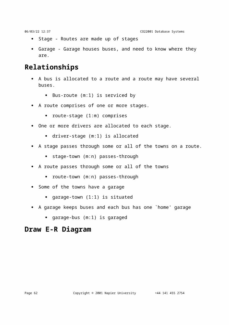
CO22001 Database Systems Student Notes
Staff(staff_no,name,address,dob, bonus, wp_skills, sales_area, car_allowance)
This represents a single entity type with no subclasses.
This is no good if the subclasses are not disjoint or if there are relationships between the subclasses and the other entities.
In addition, there will be many null fields if the subclasses do not overlap a lot. However, it avoids any joins to get additional information about each member of staff.
Dr G. Russell Copyright © 2002 Napier University Page 63

08/05/23 15:04 CO22001 Database Systems
Unit 3.1 - Normalisation 1Unit 3.1 - Normalisation What is normalisation? Normalisation is the process of taking data from a problem and reducing it to a set of relations while ensuring data integrity and eliminating data redundancy
Data integrity - all of the data in the database are consistent, and satisfies all integrity constraints.
Data redundancy – if data in the database can be found in two different locations (direct redundancy) or if data can be calculated from other data items (indirect redundancy) then the data is said to contain redundancy.
Data should only be stored once and avoid storing data that can be calculated from other data already held in the database. During the process or normalisation redundancy must be removed, but not at the expense of breaking data integrity rules.
If redundancy exists in the database then problems can arise when the database is in normal operation:
When data is inserted the data must be duplicated correctly in all places where there is redundancy. For instance, if two tables exist for in a database, and both tables contain the employee name, then creating a new employee entry requires that both tables be updated with the employee name.
When data is modified in the database, if the data being changed has redundancy, then all versions of the redundant data must be updated simultaneously. So in the employee example a change to the employee name must happen in both tables simultaneously.
The removal of redundancy helps to prevent insertion and update errors, since the data is only available in one attribute of one table in the database.
The data in the database can be considered to be in one of a number of `normal forms'. Basically the normal form of the data indicates how much redundancy is in that data. The normal forms have a strict ordering:
1. 1st Normal Form
2. 2nd Normal Form
3. 3rd Normal Form
4. BCNF
5. 4th Normal Form
Page 64 Copyright © 2001 Napier University +44 141 455 2754
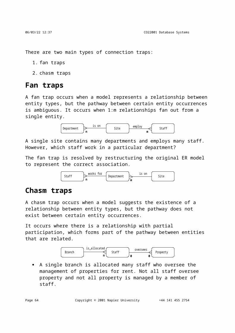
CO22001 Database Systems Student Notes
6. 5th Normal Form
To be in a particular form requires that the data meets the criteria to also be in all normal forms before that form. Thus to be in 2nd normal form the data must meet the criteria for both 2nd normal form and 1st normal form. The higher the form the more redundancy has been eliminated.
Integrity Constraints An integrity constraint is a rule that restricts the values that may be present in the database The relational data model includes constraints that are used to verify the validity of the data as well as adding meaningful structure to it:
entity integrity :
The rows (or tuples) in a relation represent entities, and each one must be uniquely identified. Hence we have the primary key that must have a unique non-null value for each row.
referential integrity :
This constraint involves the foreign keys. Foreign keys tie the relations together, so it is vitally important that the links are correct. Every foreign key must either be null or its value must be the actual value of a key in another relation.
Understanding DataSometimes the starting point for understanding data is given in the form of relations and functional dependancies. This would be the case where the starting point in the process was a detailed specification of the problem. We already know what relations are. Functional dependancies are rules stating that given a certain set of attributes (the determinant) determines a second set of attributes.
The definition of a functional dependency looks like A->B. In this case B is a single attribute but it can be as many attributes as required (for instance, X->J,K,L,M). In the functional dependency, the determinant (the left hand side of the -> sign) can determine the set of attributes on the right hand side of the -> sign. This basically means that A selects a particular value for B, and that A is unique. In the second example X is unique and selects a particular set of values for J,K,L, and M. It can also be said that B is functionally dependent on A. In addition, a particular value of A ALWAYS gives you a particular value for B, but not vice-versa.
Consider this example:
R(matric_no, firstname, surname, tutor_number, tutor_name)
tutor_number -> tutor_name
Here there is a relation R, and a functional dependency that indicates that:
Dr G. Russell Copyright © 2002 Napier University Page 65

08/05/23 15:04 CO22001 Database Systems
instances of tutor_number are unique in the data
from the data, given a tutor_number, it is always possible to work out the tutor_name.
As an example tutor number 1 may be “Mr Smith”, but tutor number 10 may also be “Mr Smith”. Given a tutor number of 1, this is ALWAYS “Mr Smith”. However, given the name “Mr Smith” it is not possible to work out if we are talking about tutor 1 or tutor 10.
There is actually a second functional dependency for this relation, which can be worked out from the relation itself. As the relation has a primary key, then given this attribute you can determine all the other attributes in R. This is an implied functional dependency and is not normally listed in the list of functional dependents.
Extracting understanding
It is possible that the relations and the determinants have not yet been defined for a problem, and therefore must be calculated from examples of the data. Consider the following Student table.
Student - an unnormalised table with repeating groups
matric_no Name date_of_birth subject grade
960100 Smith, J 14/11/1977DatabasesSoft_DevISDE
CAD
960105 White, A 10/05/1975 Soft_DevISDE
BB
960120 Moore, T 11/03/1970DatabasesSoft_DevWorkshop
ABC
960145 Smith, J 09/01/1972 Databases B
960150 Black, D 21/08/1973DatabasesSoft_DevISDEWorkshop
BDCD
The subject/grade pair is repeated for each student. 960145 has 1 pair while 960150 has four. Repeating groups are placed inside another set of parenthesizes. From the table the following relation is generated:
Student(matric_no, name, date_of_birth, ( subject, grade ) )
The repeating group needs a key in order that the relation can be correctly defined. Looking at the data one can see that grade repeats within matric_no (for instance, for 960150, the student has 2 D grades). However, subject never seems to repeat for a single matric_no, and therefore is
Page 66 Copyright © 2001 Napier University +44 141 455 2754
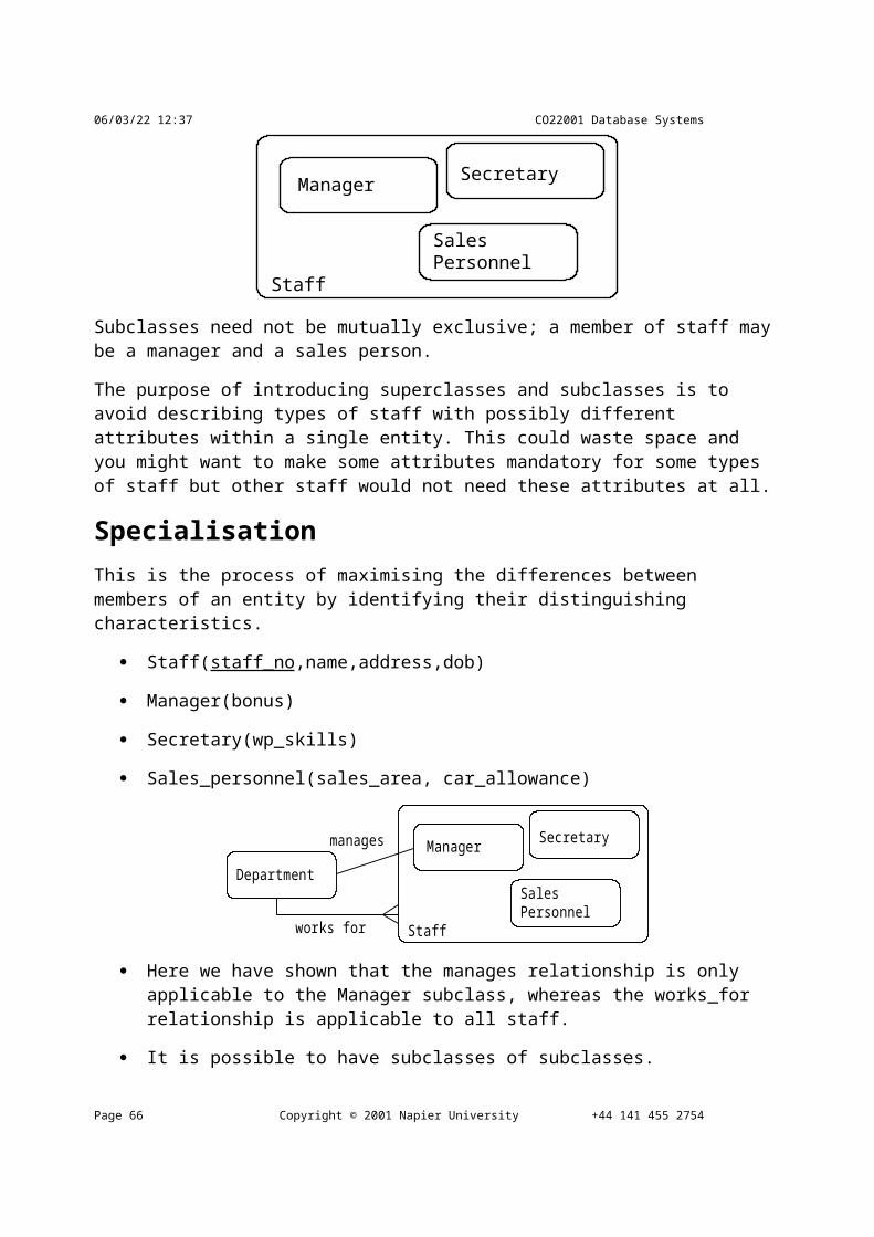
CO22001 Database Systems Student Notes
a candidate key in the repeating group.
Whenever keys or dependencies are extracted from example data, the information extracted is only as good as the data sample examined. It could be that another data sample disproves some of the key selections made or dependencies extracted. What is important however is that the information extracted during these exercises is correct for the data being examined.
Looking at the data itself, we can see that the same name appears more than once in the name column. The name in conjunction with the date_of_birth seems to be unique, suggesting a functional dependency of:
name, date_of_birth -> matric_no
This implies that not only is the matric_no sufficient to uniquely identify a student, the student’s name combined with the date of birth is also sufficient to uniquely identify a student. It is therefore possible to have the relation Student written as:
Student(matric_no, name, date_of_birth, ( subject, grade ) )
As guidance in cases where a variety of keys could be selected one should try to select the relation with the least number of attributes defined as primary keys.
Flattened TablesNote that the student table shown above explicitly identifies the repeating group. It is also possible that the table presented will be what is called a flat table, where the repeating group is not explicitly shown:
Student #2 - Flattened Table
matric_no name date_of_birth Subject grade
960100 Smith, J 14/11/1977 Databases C
960100 Smith, J 14/11/1977 Soft_Dev A
960100 Smith, J 14/11/1977 ISDE D
960105 White, A 10/05/1975 Soft_Dev B
960105 White, A 10/05/1975 ISDE B
960120 Moore, T 11/03/1970 Databases A
960120 Moore, T 11/03/1970 Soft_Dev B
960120 Moore, T 11/03/1970 Workshop C
960145 Smith, J 09/01/1972 Databases B
960150 Black, D 21/08/1973 Databases B
Dr G. Russell Copyright © 2002 Napier University Page 67
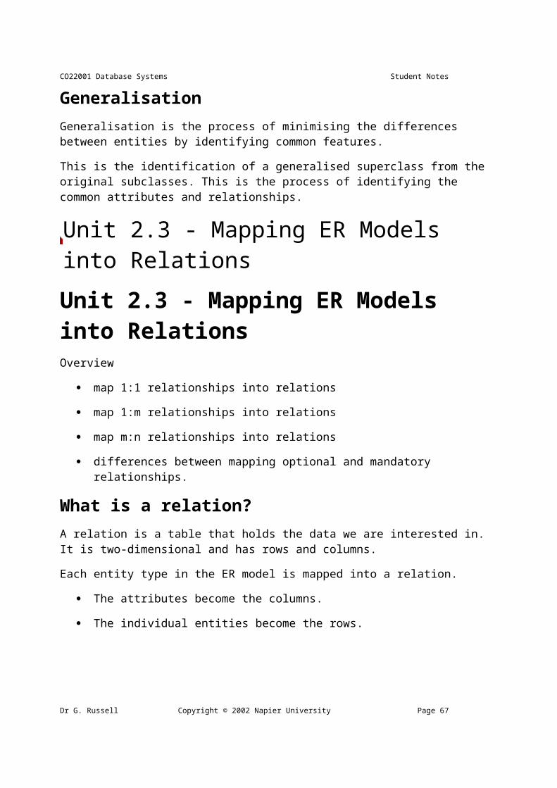
08/05/23 15:04 CO22001 Database Systems
960150 Black, D 21/08/1973 Soft_Dev D
960150 Black, D 21/08/1973 ISDE C
960150 Black, D 21/08/1973 Workshop B
The table still shows the same data as the previous example, but the format is different. We have removed the repeating group (which is good) but we have introduced redundancy (which is bad).
Sometimes you will miss spotting the repeating group, so you may produce something like the following relation for the Student data.
Student(matric_no, name, date_of_birth, subject, grade )
matric_no -> name, date_of_birth name, date_of_birth -> matric_no
This data does not explicitly identify the repeating group, but as you will see the result of the normalisation process on this relation produces exactly the same relations as the normalisation of the version that explicitly does have a repeating group.
First Normal Form First normal form (1NF) deals with the `shape' of the record type
A relation is in 1NF if, and only if, it contains no repeating attributes or groups of attributes.
Example:
The Student table with the repeating group is not in 1NF
It has repeating groups, and it is called an `unnormalised table'.
Relational databases require that each row only has a single value per attribute, and so a repeating group in a row is not allowed.
To remove the repeating group, one of two things can be done:
either flatten the table and extend the key, or
decompose the relation- leading to First Normal Form
Flatten table and Extend Primary Key The Student table with the repeating group can be written as:
Page 68 Copyright © 2001 Napier University +44 141 455 2754
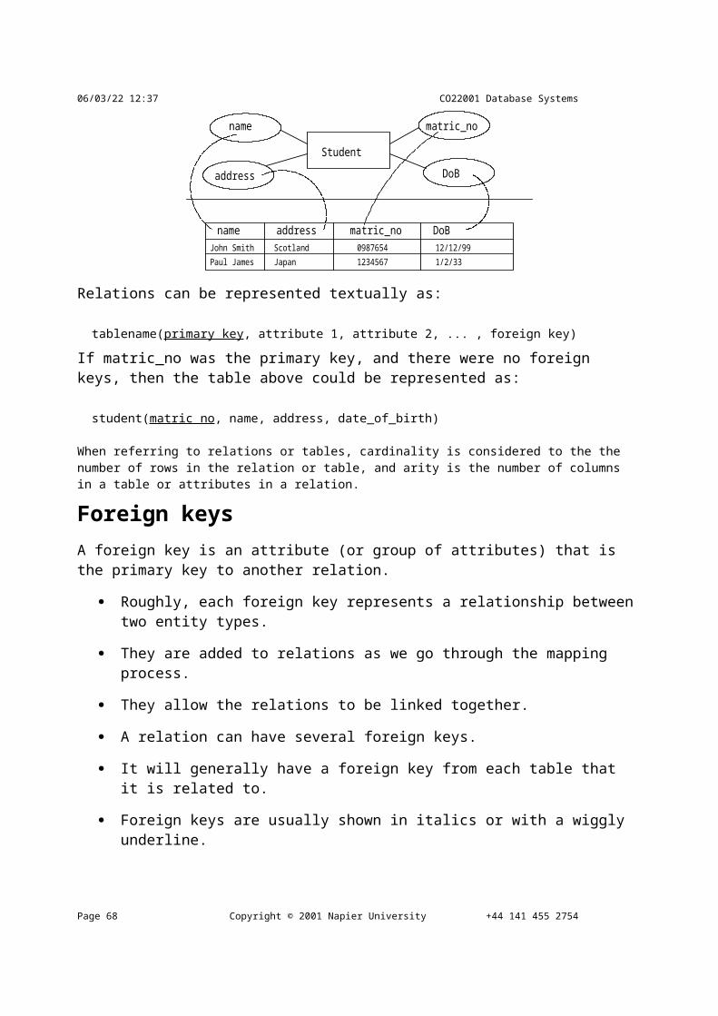
CO22001 Database Systems Student Notes
Student(matric_no, name, date_of_birth, ( subject, grade ) )
If the repeating group was flattened, as in the Student #2 data table, it would look something like:
Student(matric_no, name, date_of_birth, subject, grade )
Although this is an improvement, we still have a problem. matric_no can no longer be the primary key - it does not have an unique value for each row. So we have to find a new primary key - in this case it has to be a compound key since no single attribute can uniquely identify a row. The new primary key is a compound key (matrix_no + subject).
We have now solved the repeating groups problem, but we have created other complications. Every repetition of the matric_no, name, and data_of_birth is redundant and liable to produce errors.
With the relation in its flattened form, strange anomalies appear in the system. Redundant data is the main cause of insertion, deletion, and updating anomalies.
Insertion anomaly:
With the primary key including subject, we cannot enter a new student until they have at least one subject to study. We are not allowed NULLs in the primary key so we must have an entry in both matric_no and subject before we can create a new record.
This is known as the insertion anomaly. It is difficult to insert new records into the database.
On a practical level, it also means that it is difficult to keep the data up to date.
Update anomaly
If the name of a student were changed
for example Smith, J. was changed to Green, J.
this would require not one change but many
one for every subject that Smith, J. studied.
Deletion anomaly
If all of the records for the `Databases' subject were deleted from the table,we would inadvertently lose all of the information on the student with matric_no 960145.
o This would be the same for any student who was studying only one subject and the subject was deleted.
o Again this problem arises from the need to have a compound primary key.
Dr G. Russell Copyright © 2002 Napier University Page 69

08/05/23 15:04 CO22001 Database Systems
Decomposing the relation The alternative approach is to split the table into two parts, one for the repeating groups
and one of the non-repeating groups.
the primary key for the original relation is included in both of the new relations
Page 70 Copyright © 2001 Napier University +44 141 455 2754
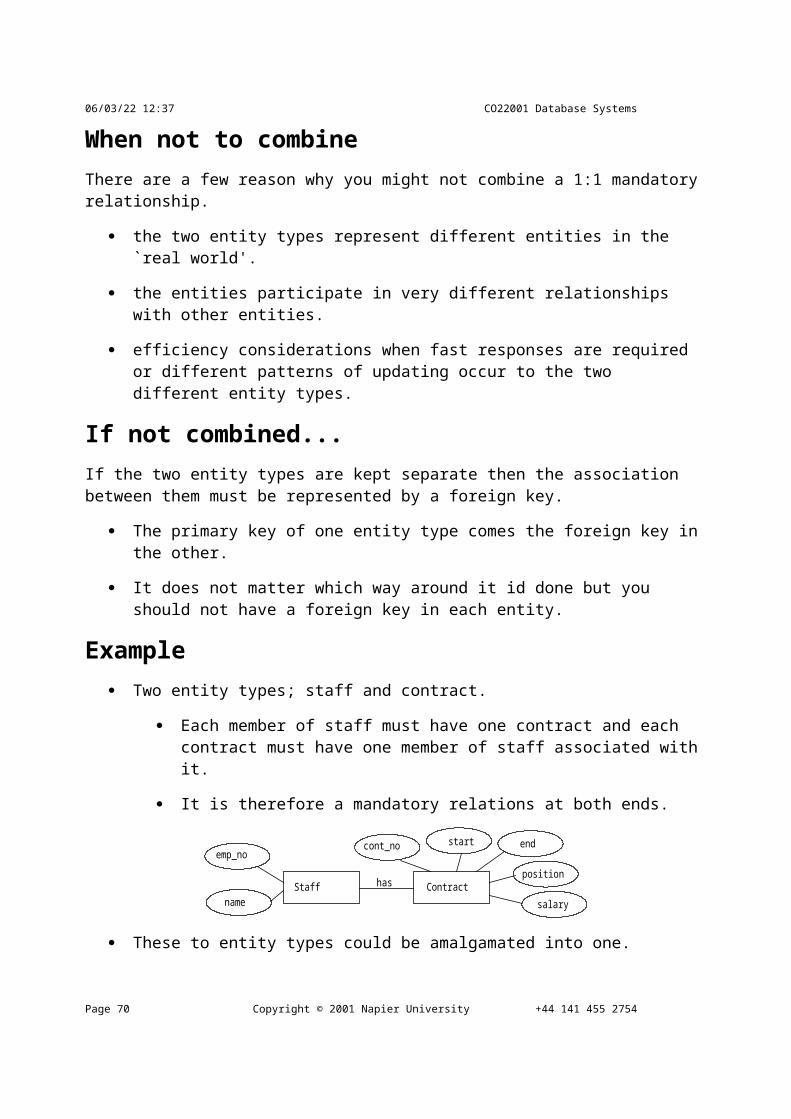
CO22001 Database Systems Student Notes
Record
matric_no subject grade
960100 Databases C
960100 Soft_Dev A
960100 ISDE D
960105 Soft_Dev B
960105 ISDE B
... ... ...
960150 Workshop B
Student
matric_no name date_of_birth
960100 Smith,J 14/11/1977
960105 White,A 10/05/1975
960120 Moore,T 11/03/1970
960145 Smith,J 09/01/1972
960150 Black,D 21/08/1973
We now have two relations, Student and Record.
Student contains the original non-repeating groups
Record has the original repeating groups and the matric_no
Student(matric_no, name, date_of_birth )Record(matric_no, subject, grade )
Matric_no remains the key to the Student relation. It cannot be the complete key to the new Record relation - we end up with a compound primary key consisting of matric_no and subject. The matric_no is the link between the two tables - it will allow us to find out which subjects a student is studying . So in the Record relation, matric_no is the foreign key.
Dr G. Russell Copyright © 2002 Napier University Page 71

08/05/23 15:04 CO22001 Database Systems
This method has eliminated some of the anomalies. It does not always do so, it depends on the example chosen
In this case we no longer have the insertion anomaly
It is now possible to enter new students without knowing the subjects that they will be studying
They will exist only in the Student table, and will not be entered in the Record table until they are studying at least one subject.
We have also removed the deletion anomaly
If all of the `databases' subject records are removed, student 960145 still exists in the Student table.
We have also removed the update anomaly
Student and Record are now in First Normal Form.
Second Normal Form Second normal form (or 2NF) is a more stringent normal form defined as:
A relation is in 2NF if, and only if, it is in 1NF and every non-key attribute is fully functionally dependent on the whole key.
Thus the relation is in 1NF with no repeating groups, and all non-key attributes must depend on the whole key, not just some part of it. Another way of saying this is that there must be no partial key dependencies (PKDs).
The problems arise when there is a compound key, e.g. the key to the Record relation - matric_no, subject. In this case it is possible for non-key attributes to depend on only part of the key - i.e. on only one of the two key attributes. This is what 2NF tries to prevent.
Consider again the Student relation from the flattened Student #2 table: Student(matric_no, name, date_of_birth, subject, grade )
There are no repeating groups
The relation is already in 1NF
However, we have a compound primary key - so we must check all of the non-key attributes against each part of the key to ensure they are functionally dependent on it.
matric_no determines name and date_of_birth, but not grade.
subject together with matric_no determines grade, but not name or date_of_birth.
So there is a problem with potential redundancies
Page 72 Copyright © 2001 Napier University +44 141 455 2754
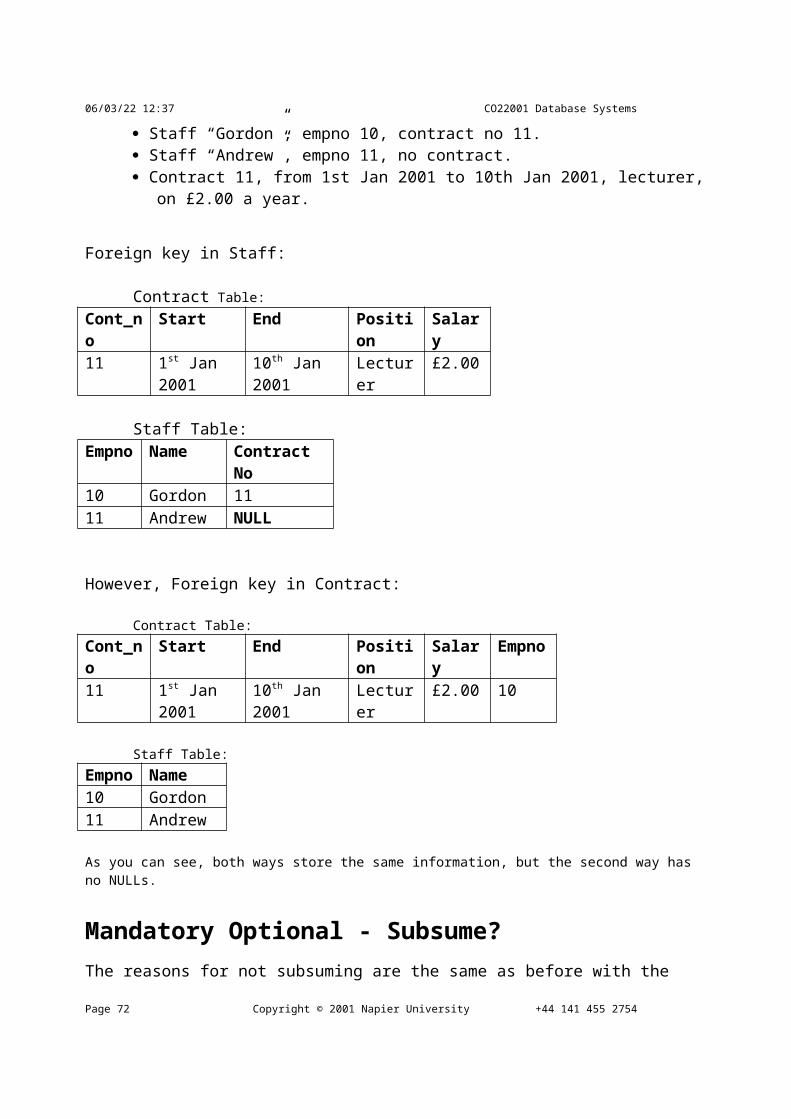
CO22001 Database Systems Student Notes
A dependency diagram is used to show how non-key attributes relate to each part or combination of parts in the primary key.
This relation is not in 2NF
It appears to be two tables squashed into one.
the solutions is to split the relation up into its component parts.
separate out all the attributes that are solely dependent on matric_no
put them in a new Student_details relation, with matric_no as the primary key
separate out all the attributes that are solely dependent on subject.
in this case no attributes are solely dependent on subject.
separate out all the attributes that are solely dependent on matric_no + subject
put them into a separate Student relation, keyed on matric_no + subject
Dr G. Russell Copyright © 2002 Napier University Page 73
matric_no gradesubjectdate_of_bithname
Student
PKD
Fully Dependent
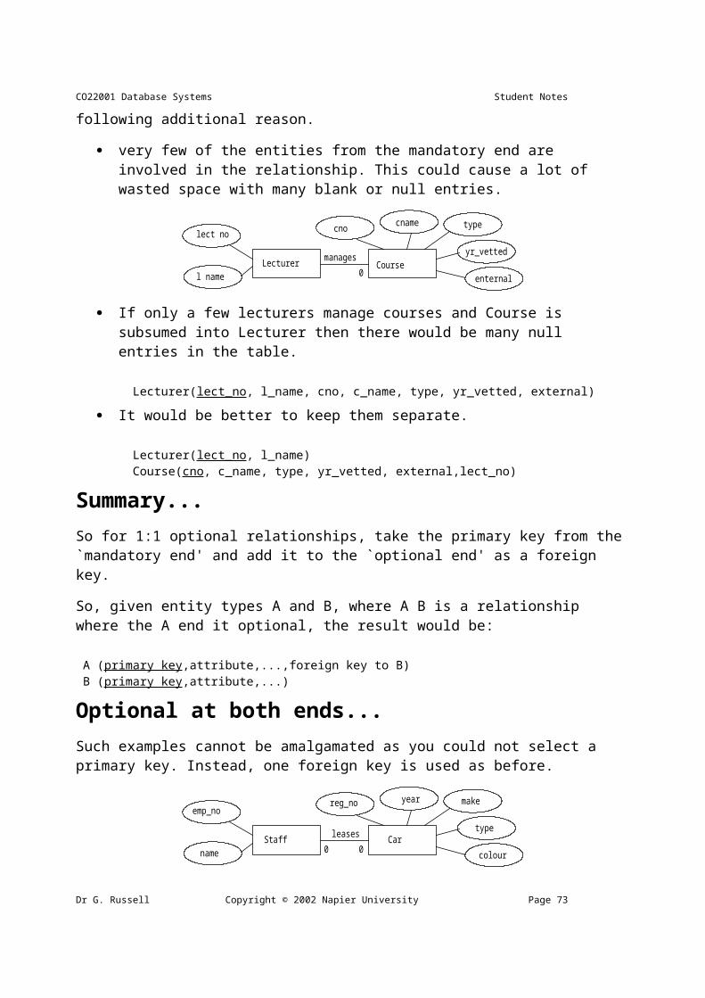
08/05/23 15:04 CO22001 Database Systems
All attributes in each relation are fully functionally dependent upon its primary key
These relations are now in 2NF
Interestingly this is the same set of relations as when we recognized that there were repeating terms in the table and directly removed the repeating terms. It should not really matter what process you followed when normalizing, as the end result should be similar relations.
Third Normal Form 3NF is an even stricter normal form and removes virtually all the redundant data :
A relation is in 3NF if, and only if, it is in 2NF and there are no transitive functional dependencies
Transitive functional dependencies arise:
when one non-key attribute is functionally dependent on another non-key attribute:
FD: non-key attribute -> non-key attribute
and when there is redundancy in the database
By definition transitive functional dependency can only occur if there is more than one non-key field, so we can say that a relation in 2NF with zero or one non-key field must automatically be in 3NF.
Page 74 Copyright © 2001 Napier University +44 141 455 2754
Student Details
matrix_no name date_of_birth
Student
matrix_no subject grade
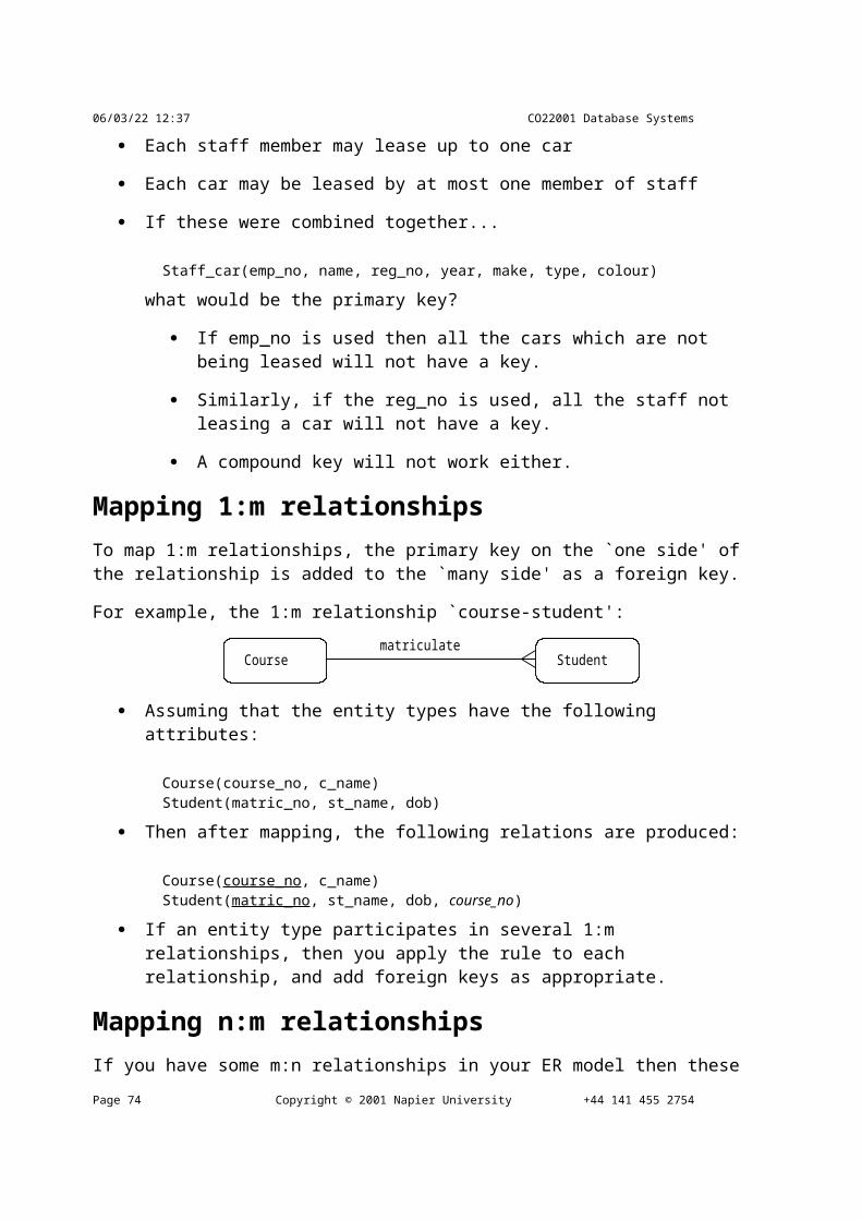
CO22001 Database Systems Student Notes
project_no manager address
Project has more than one non-key field so we must check for transitive dependency:
p1 Black,B 32 High Street
p2 Smith,J 11 New Street
p3 Black,B 32 High Street
p4 Black,B 32 High Street
address depends on the value in the manager column
every time B Black is listed in the manager column, the address column has the value `32 High Street'. From this the relation and functional dependency can be implied as:
Project(project_no, manager, address)
manager -> address
in this case address is transitively dependent on manager. Manager is the determinant - it determines the value of address. It is transitive functional dependency only if all attributes on the left of the “->” are not in the key but are all in the relation, and all attributes to the right of the “->” are not in the key with at least one actually being in the relation.
Data redundancy arises from this
we duplicate address if a manager is in charge of more than one project
causes problems if we had to change the address- have to change several entries, and this could lead to errors.
Eliminate transitive functional dependency by splitting the table
create two relations - one with the transitive dependency in it, and another for all of the remaining attributes.
split Project into Project and Manager.
the determinant attribute becomes the primary key in the new relation
manager becomes the primary key to the Manager relation
the original key is the primary key to the remaining non-transitive attributes
in this case, project_no remains the key to the new Projects table.
Project project_no manager
Dr G. Russell Copyright © 2002 Napier University Page 75
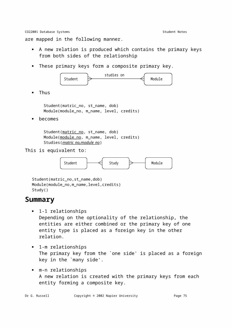
08/05/23 15:04 CO22001 Database Systems
p1 Black,B
p2 Smith,J
p3 Black,B
p4 Black,B
Manager manager address
Black,B 32 High Street
Smith,J 11 New Street
Now we need to store the address only once
If we need to know a manager's address we can look it up in the Manager relation
The manager attribute is the link between the two tables, and in the Projects table it is now a foreign key.
These relations are now in third normal form.
Summary: 1NF A relation is in 1NF if it contains no repeating groups
To convert an unnormalised relation to 1NF either:
Flatten the table and change the primary key, or
Decompose the relation into smaller relations, one for the repeating groups and one for the non-repeating groups.
Remember to put the primary key from the original relation into both new relations.
This option is liable to give the best results.
Summary: 2NF A relation is in 2NF if it contains no repeating groups and no partial key functional
dependencies
Rule: A relation in 1NF with a single key field must be in 2NF
Page 76 Copyright © 2001 Napier University +44 141 455 2754

CO22001 Database Systems Student Notes
To convert a relation with partial functional dependencies to 2NF. create a set of new relations:
One relation for the attributes that are fully dependent upon the key.
One relation for each part of the key that has partially dependent attributes
Summary: 3NF A relation is in 3NF if it contains no repeating groups, no partial functional
dependencies, and no transitive functional dependencies
To convert a relation with transitive functional dependencies to 3NF, remove the attributes involved in the transitive dependency and put them in a new relation
Rule: A relation in 2NF with only one non-key attribute must be in 3NF
In a normalised relation a non-key field must provide a fact about the key, the whole key and nothing but the key.
Relations in 3NF are sufficient for most practical database design problems. However, 3NF does not guarantee that all anomalies have been removed.
Unit 3.2 - Normalisation 2Unit 3.2 - Normalisation Continued Overview
normalise a relation to Boyce Codd Normal Form (BCNF)
normalise a relation to forth normal form (4NF)
normalise a relation to fifth normal form (5NF)
Boyce-Codd Normal Form (BCNF) When a relation has more than one candidate key, anomalies may result even
though the relation is in 3NF.
3NF does not deal satisfactorily with the case of a relation with overlapping candidate keys
i.e. composite candidate keys with at least one attribute in common.
BCNF is based on the concept of a determinant.
A determinant is any attribute (simple or composite) on which some other attribute is fully functionally dependent.
Dr G. Russell Copyright © 2002 Napier University Page 77
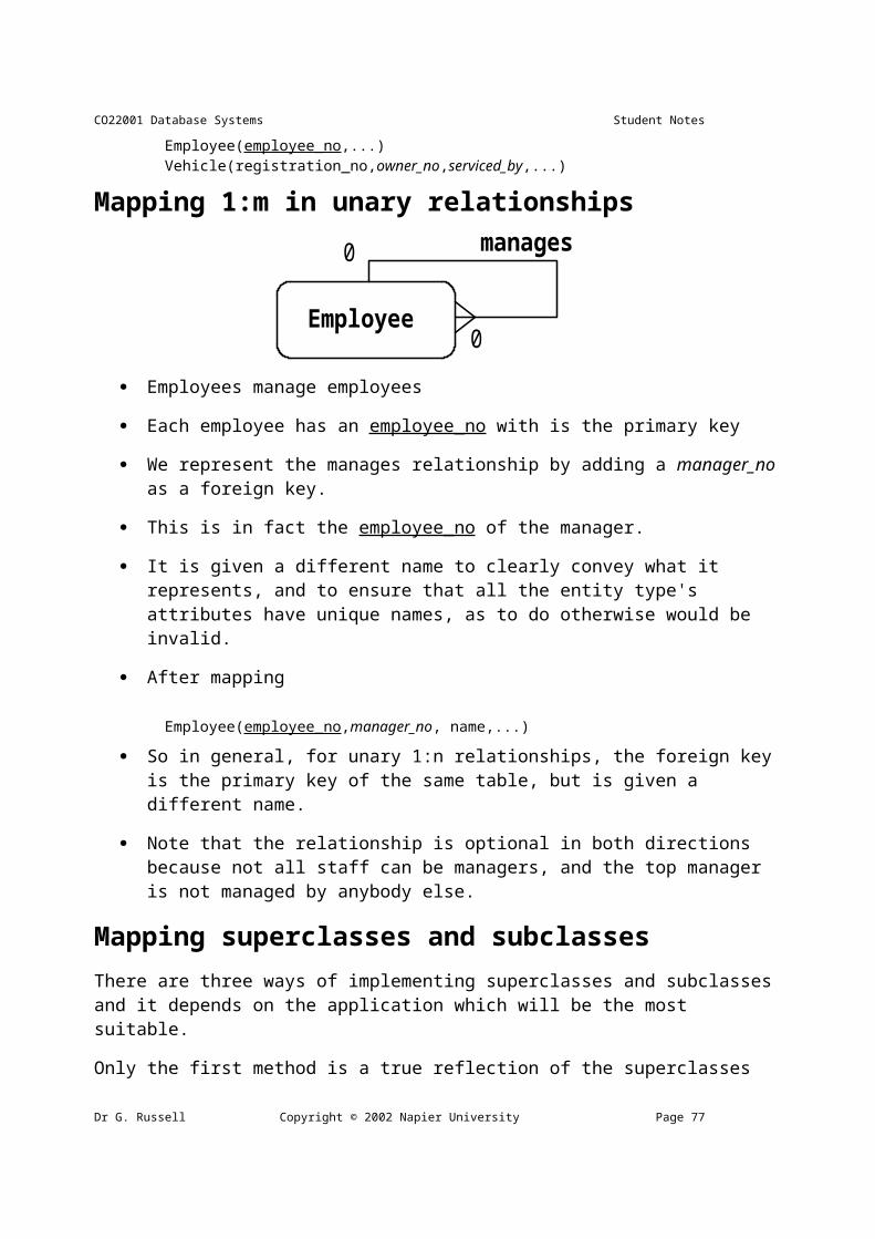
08/05/23 15:04 CO22001 Database Systems
A relation is in BCNF is, and only if, every determinant is a candidate key.
Consider the following relation and determinants.
R(a,b,c,d)a,c -> b,da,d -> b
Here, the first determinant suggests that the primary key of R could be changed from a,b to a,c. If this change was done all of the non-key attributes present in R could still be determined, and therefore this change is legal. However, the second determinant indicates that a,d determines b, but a,d could not be the key of R as a,d does not determine all of the non key attributes of R (it does not determine c). We would say that the first determinate is a candidate key, but the second determinant is not a candidate key, and thus this relation is not in BCNF (but is in 3rd normal form).
Normalisation to BCNF - Example 1
Patient No
Patient Name Appointment Id Time Doctor
1 John 0 09:00 Zorro
2 Kerr 0 09:00 Killer
3 Adam 1 10:00 Zorro
4 Robert 0 13:00 Killer
5 Zane 1 14:00 Zorro
Lets consider the database extract shown above. This depicts a special dieting clinic where the each patient has 4 appointments. On the first they are weighed, the second they are exercised, the third their fat is removed by surgery, and on the fourth their mouth is stitched closed… Not all patients need all four appointments! If the Patient Name begins with a letter before “P” they get a morning appointment, otherwise they get an afternoon appointment. Appointment 1 is either 09:00 or 13:00, appointment 2 10:00 or 14:00, and so on. From this (hopefully) make-believe scenario we can extract the following determinants:
Page 78 Copyright © 2001 Napier University +44 141 455 2754

CO22001 Database Systems Student Notes
DB(Patno,PatName,appNo,time,doctor)
Patno -> PatNamePatno,appNo -> Time,doctorTime -> appNo
Now we have to decide what the primary key of DB is going to be. From the information we have, we could chose: DB(Patno,PatName,appNo,time,doctor) (example 1a)or DB(Patno,PatName,appNo,time,doctor) (example 1b)
patient names and G.P. names are not unique
hospital names are unique
consultants have one unique phone number
on a given day a consultant attends just one hospital
on a given day a patient will have just one appointment with a given consultant
consultant names are unique
From the table and the additional list of specified constraints we can extract the starting relation and the determinants.
Dr G. Russell Copyright © 2002 Napier University Page 79
08/05/23 15:04 CO22001 Database Systems
Unnormalised
Patient(Example 1a - DB(Patno,PatName,appNo,time,doctor)
1NF Eliminate repeating groups.
None:
DB(Patno,PatName,appNo,time,doctor)
2NF Eliminate partial key dependencies DB(Patno,appNo,time,doctor)R1(Patno,PatName)
3NF Eliminate transitive dependencies None: so just as 2NF
BCNF Every determinant is a candidate key DB(Patno,appNo,time,doctor) R1(Patno,PatName)
Go through all determinates where ALL of the left hand attributes are present in a relation and at least ONE of the right hand attributes are also present in the relation.
Patno -> PatNamePatno is present in DB, but not PatName, so not relevant.
Patno,appNo -> Time,doctorAll LHS present, and time and doctor also present, so relevant. Is this a candidate key? Patno,appNo IS the key, so this is a candidate key. Thus this is OK for BCNF compliance.
Time -> appNoTime is present, and so is appNo, so relevant. Is this a candidate key. If it was then we could rewrite DB as: DB(Patno,appNo,time,doctor)This will not work, as you need both time and Patno together to form a unique key. Thus this determinate is not a candidate key, and therefore DB is not in BCNF. We need to fix this.
BCNF: rewrite to DB(Patno,time,doctor) R1(Patno,PatName) R2(time,appNo)
time is enough to work out the appointment number of a patient. Now BCNF is satisfied, and the final relations shown are in BCNF.
Page 80 Copyright © 2001 Napier University +44 141 455 2754

CO22001 Database Systems Student Notes
Example 1b - DB(Patno,PatName,appNo,time,doctor)
1NF Eliminate repeating groups.
None:
DB(Patno,PatName,appNo,time,doctor)
2NF Eliminate partial key dependencies DB(Patno,time,doctor)R1(Patno,PatName)R2(time,appNo)
3NF Eliminate transitive dependencies None: so just as 2NF
BCNF Every determinant is a candidate key DB(Patno,appNo,time,doctor) R1(Patno,PatName)
Go through all determinates where ALL of the left hand attributes are present in a relation and at least ONE of the right hand attributes are also present in the relation.
Patno -> PatNamePatno is present in DB, but not PatName, so not relevant.
Patno,appNo -> Time,doctorNot all LHS present, so not relevant.
Time -> appNoTime is present, and so is appNo, so relevant. Is this a candidate key. However, is the key and determinant for R2, so it is OK for BCNF.
BCNF: as 3NF DB(Patno,time,doctor) R1(Patno,PatName) R2(time,appNo)
Summary - Example 1
This example has demonstrated three things:
1. BCNF is stronger than 3NF, relations that are in 3NF are not necessarily in BCNF
2. BCNF is needed in certain situations to obtain full understanding of the data model
3. there are several routes to take to arrive at the same set of relations in BCNF.
Dr G. Russell Copyright © 2002 Napier University Page 81

08/05/23 15:04 CO22001 Database Systems
Unfortunately there are no rules as to which route will be the easiest one to take.
Example 2 Grade_report(StudNo,StudName,(Major,Adviser, (CourseNo,Ctitle,InstrucName,InstructLocn,Grade)))
Functional dependencies
StudNo -> StudName CourseNo -> Ctitle,InstrucName InstrucName -> InstrucLocn StudNo,CourseNo,Major -> Grade StudNo,Major -> Advisor Advisor -> Major
Unnormalised
Grade_report(StudNo,StudName,(Major,Advisor, (CourseNo,Ctitle,InstrucName,InstructLocn,Grade)))
1NF Remove repeating groups
Student(StudNo,StudName)StudMajor(StudNo,Major,Advisor)StudCourse(StudNo,Major,CourseNo, Ctitle,InstrucName,InstructLocn,Grade)
2NF Remove partial key dependencies
Student(StudNo,StudName)StudMajor(StudNo,Major,Advisor)StudCourse(StudNo,Major,CourseNo,Grade)Course(CourseNo,Ctitle,InstrucName,InstructLocn)
3NF Remove transitive dependencies
Student(StudNo,StudName)StudMajor(StudNo,Major,Advisor)StudCourse(StudNo,Major,CourseNo,Grade)Course(CourseNo,Ctitle,InstrucName)Instructor(InstructName,InstructLocn)
BCNF Every determinant is a candidate key
Student : only determinant is StudNo
StudCourse: only determinant is StudNo,Major
Course: only determinant is CourseNo
Instructor: only determinant is InstrucName
StudMajor: the determinants are
Page 82 Copyright © 2001 Napier University +44 141 455 2754
CO22001 Database Systems Student Notes
StudNo,Major, or
Adviser
Only StudNo,Major is a candidate key.
BCNF
Student(StudNo,StudName)StudCourse(StudNo,Major,CourseNo,Grade)Course(CourseNo,Ctitle,InstrucName)Instructor(InstructName,InstructLocn)StudMajor(StudNo,Advisor)Adviser(Adviser,Major)
Problems BCNF overcomes STUDENT MAJOR ADVISOR
123 PHYSICS EINSTEIN
123 MUSIC MOZART
456 BIOLOGY DARWIN
789 PHYSICS BOHR
999 PHYSICS EINSTEIN
If the record for student 456 is deleted we lose not only information on student 456 but also the fact that DARWIN advises in BIOLOGY
we cannot record the fact that WATSON can advise on COMPUTING until we have a student majoring in COMPUTING to whom we can assign WATSON as an advisor.
In BCNF we have two tables:
STUDENT ADVISOR
123 EINSTEIN
123 MOZART
456 DARWIN
789 BOHR
999 EINSTEIN
Dr G. Russell Copyright © 2002 Napier University Page 83
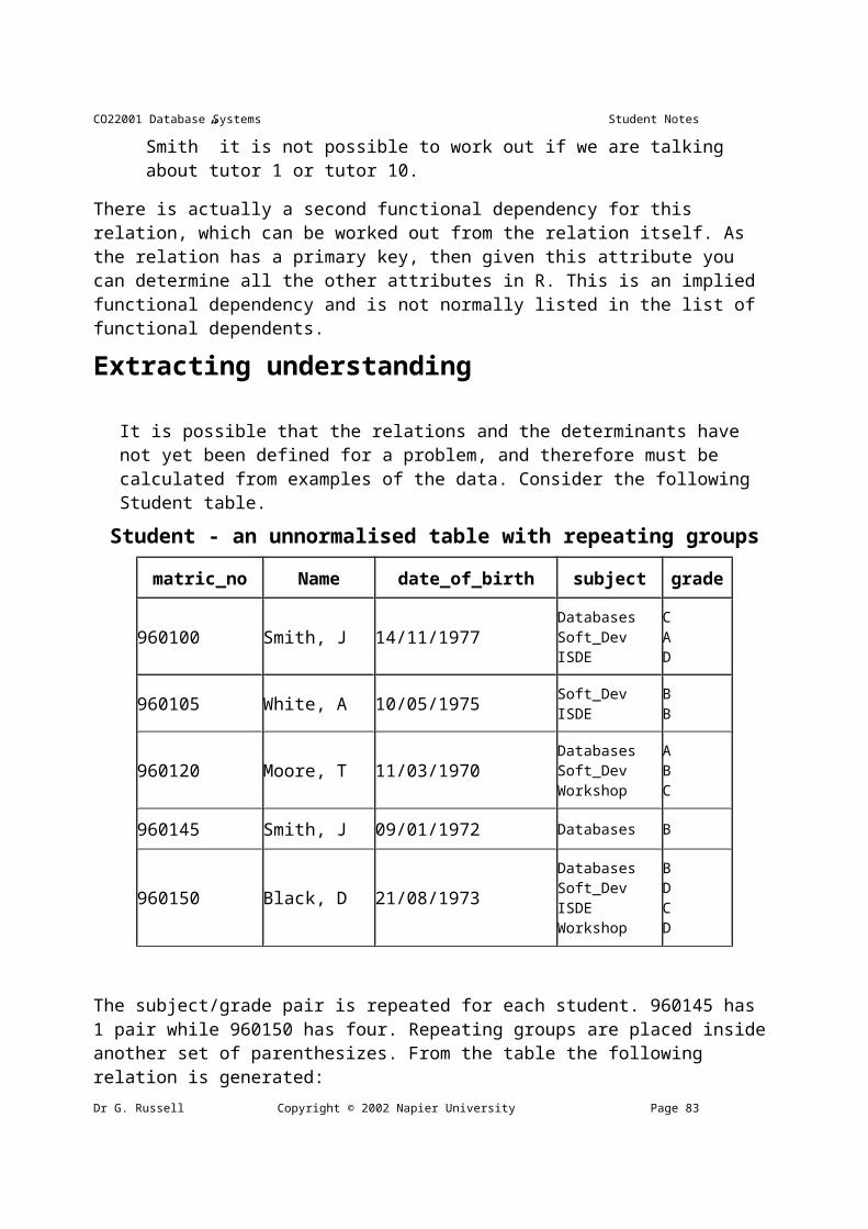
08/05/23 15:04 CO22001 Database Systems
ADVISOR MAJOR
EINSTEIN PHYSICS
MOZART MUSIC
DARWIN BIOLOGY
BOHR PHYSICS
Fourth Normal Form Under 4NF, a record type should not contain two or more independent multi-valued facts about an entity. Note that 4NF and 5NF are not examinable, and are shown here for completeness. They should never occur using the approaches you have been taught in this module, but can occur if you were taking over a database project where poor design techniques were involved or where redundancy was deliberately introduced for some reason.
A relation is in 4NF if it is in BCNF and it contains no multi-valued dependencies.
A multi-valued fact may correspond to a many-many relationship or to a many-one relationship.
A multi-valued dependency exists when there are three attributes (e.g. A,B, and C) in a relation, and for each value of A there is a well-defined set of valued B and a well defined set of values C. However, the set of values of B is independent of set C and vice-versa.
Example Consider information stored about movie stars. It includes details of their various
addresses and the movies they starred in:
Name - Address
Name - Movie
Page 84 Copyright © 2001 Napier University +44 141 455 2754

CO22001 Database Systems Student Notes
Name Street City Title Year
C. Fisher 123 Maple St. Hollywood Star Wars 1977
C. Fisher 5 Locust Ln. Malibu Star Wars 1977
C. Fisher 123 Maple St. Hollywood Empire Strikes Back 1980
C. Fisher 5 Locust Ln. Malibu Empire Strikes Back 1980
C. Fisher 123 Maple St. Hollywood Return of the Jedi 1983
C. Fisher 5 Locust Ln. Malibu Return of the Jedi 1983
Carrie Fisher has two addresses and has been in three movies
The only way to express the fact that addresses and movies are independent is to have each address appear with each movie
but this has introduced redundancy
There is no BCNF violation
But the relation is not in 4NF
We need to break it up into 2 tables
Name Street City
C. Fisher 123 Maple St. Hollywood
C. Fisher 5 Locust Ln. Malibu
Name Title Year
C.Fisher Star Wars 1977
C.Fisher Empire Strikes Back 1980
C.Fisher Return of the Jedi 1983
Fifth Normal Form 5NF is designed to cope with a type of dependency called join dependency
A relation that has a join dependency cannot be decomposed by a projection into other relations without spurious results
Dr G. Russell Copyright © 2002 Napier University Page 85
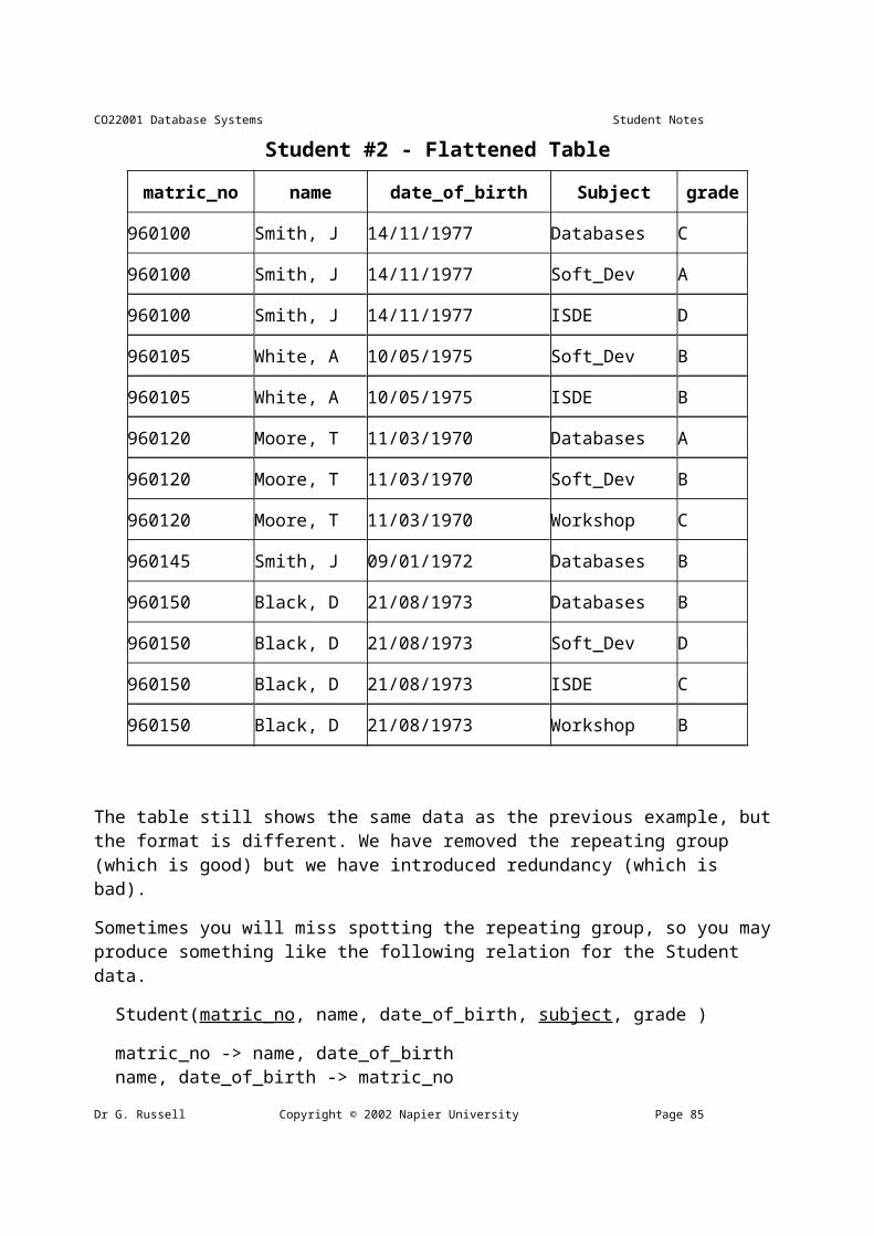
08/05/23 15:04 CO22001 Database Systems
a relation is in 5NF when its information content cannot be reconstructed from several smaller relations
i.e. from relations having fewer attributes than the original relation
Join Dependency Decomposition
Name Language Hobby
Name Language Name Hobby
C. Fisher French Cooks C. Fisher French C. Fisher Cooks
C. Fisher Spanish Cooks C. Fisher Spanish C. Fisher Writes
C. Fisher English Writes C. Fisher English M. Brown Read
M. Brown Spanish Read M. Brown Spanish M. Brown Cook
M. Brown Italian Cook M. Brown Italian K. Clark Cook
K. Clark Italian Cook K. Clark Italian K. Clark Decorating
K. Clark Japanese Decorating K. Clark Japanese
Spurious results
Name Language Hobby Name Language Hobby
C. Fisher French Cooks M. Brown Spanish Cook
C. Fisher French Writes M. Brown Italian Read
C. Fisher Spanish Cooks M. Brown Italian Cook
C. Fisher Spanish Writes K. Clark Italian Cook
C. Fisher English Cooks K. Clark Italian Decorating
C. Fisher English Writes K. Clark Japanese Cook
M. Brown Spanish Read K. Clark Japanese Decorating
Returning to the ER Model Now that we have reached the end of the normalisation process, you must go back
and compare the resulting relations with the original ER model
You may need to alter it to take account of the changes that have occurred Page 86 Copyright © 2001 Napier University +44 141 455 2754

CO22001 Database Systems Student Notes
during the normalisation process Your ER diagram should always be a prefect reflection of the model you are going to implement in the database, so keep it up to date!
The changes required depends on how good the ER model was at first!
Unit 3.3 - Relational Algebra 1Unit 3.3 - Relational Algebra In order to implement a DBMS, there must exist a set of rules which state how the database system will behave. For instance, somewhere in the DBMS must be a set of statements which indicate than when someone inserts data into a row of a relation, it has the effect which the user expects. One way to specify this is to use words to write an `essay' as to how the DBMS will operate, but words tend to be imprecise and open to interpretation. Instead, relational databases are more usually defined using Relational Algebra.
Relational Algebra is :
the formal description of how a relational database operates
an interface to the data stored in the database itself
the mathematics which underpin SQL operations
Operators in relational algebra are not necessarily the same as SQL operators, even if they have the same name. For example, the SELECT statement exists in SQL, and also exists in relational algebra. These two uses of SELECT are not the same. The DBMS must take whatever SQL statements the user types in and translate them into relational algebra operations before applying them to the database.
Terminology Relation - a set of tuples.
Tuple - a collection of attributes which describe some real world entity.
Attribute - a real world role played by a named domain.
Domain - a set of atomic values.
Set - a mathematical definition for a collection of objects which contains no duplicates.
Operators - Write INSERT - provides a list of attribute values for a new tuple in a relation. This
operator is the same as SQL.
Dr G. Russell Copyright © 2002 Napier University Page 87

08/05/23 15:04 CO22001 Database Systems
DELETE - provides a condition on the attributes of a relation to determine which tuple(s) to remove from the relation. This operator is the same as SQL.
MODIFY - changes the values of one or more attributes in one or more tuples of a relation, as identified by a condition operating on the attributes of the relation. This is equivalent to SQL UPDATE.
Operators - Retrieval There are two groups of operations:
Mathematical set theory based relations:UNION, INTERSECTION, DIFFERENCE, and CARTESIAN PRODUCT.
Special database operations:SELECT (not the same as SQL SELECT), PROJECT, and JOIN.
Relational SELECT SELECT is used to obtain a subset of the tuples of a relation that satisfy a select condition.
For example, find all employees born after 1st Jan 1950:
SELECTdob '01/JAN/1950'(employee)
Relational PROJECT The PROJECT operation is used to select a subset of the attributes of a relation by specifying the names of the required attributes.
For example, to get a list of all employees surnames and employee numbers:
PROJECTsurname,empno(employee)
SELECT and PROJECT SELECT and PROJECT can be combined together. For example, to get a list of employee numbers for employees in department number 1:
FROM employeeWHERE depno = 1;
SELECT empno
PROJECT empno (SELECT depno = 1 (employee))
Mapping this back to SQL gives:
Set Operations - semantics Consider two relations R and S.
Page 88 Copyright © 2001 Napier University +44 141 455 2754
CO22001 Database Systems Student Notes
UNION of R and Sthe union of two relations is a relation that includes all the tuples that are either in R or in S or in both R and S. Duplicate tuples are eliminated.
INTERSECTION of R and Sthe intersection of R and S is a relation that includes all tuples that are both in R and S.
DIFFERENCE of R and Sthe difference of R and S is the relation that contains all the tuples that are in R but that are not in S.
SET Operations - requirements For set operations to function correctly the relations R and S must be union compatible. Two relations are union compatible if
they have the same number of attributes
the domain of each attribute in column order is the same in both R and S.
UNION Example
BC
F4
22
A
DE
E
1
354
RA 1BDFE
2345
SACDE 4
321
R UNION S
Dr G. Russell Copyright © 2002 Napier University Page 89

08/05/23 15:04 CO22001 Database Systems
INTERSECTION Example
A 1C 2D 3E 4
E 5F 4D 3B 2A 1
A 1D 3
R
S
R |NTERSECTION S
DIFFERENCE Example
A 1C 2D 3E 4
E 5F 4D 3B 2A 1
C 2E 4
B 2F 4E 5
R
S
R DIFFERENCE S
S DIFFERENCE R
CARTESIAN PRODUCT The Cartesian Product is also an operator which works on two sets. It is sometimes called the CROSS PRODUCT or CROSS JOIN.
It combines the tuples of one relation with all the tuples of the other relation.
Page 90 Copyright © 2001 Napier University +44 141 455 2754

CO22001 Database Systems Student Notes
CARTESIAN PRODUCT example
E 5F 4D 3B 2A 1
A 1C 2D 3E 4
A 1 A 1C 2D 3E 4
B 2 A 1C 2D 3E 4A 1C 2D 3E 4
F 4 A 1C 2D 3E 4
E 5 A 1C 2D 3E 4
D 3
A 1A 1A 1
B 2B 2B 2
D 3D 3D 3
F 4F 4F 4
E 5E 5E 5
R
S
R CROSS S
JOIN Operator JOIN is used to combine related tuples from two relations:
In its simplest form the JOIN operator is just the cross product of the two relations.
As the join becomes more complex, tuples are removed within the cross product to make the result of the join more meaningful.
JOIN allows you to evaluate a join condition between the attributes of the relations on which the join is undertaken.
The notation used is
R JOINjoin condition S
JOIN Example
E 5F 4D 3B 2A 1
A 1C 2D 3E 4
R JOIN R.ColA = S.SColA S
A 1
A 1B 2
A 1D 3E 5
D 3E 4
E 4
A 1C 2
D 3F 4
D 3
ColA ColB
SColBSColAS
R
R JOIN R.ColB = S.SColB S
Natural Join Invariably the JOIN involves an equality test, and thus is often described as an equi-join.
Dr G. Russell Copyright © 2002 Napier University Page 91

08/05/23 15:04 CO22001 Database Systems
Such joins result in two attributes in the resulting relation having exactly the same value. A `natural join' will remove the duplicate attribute(s).
In most systems a natural join will require that the attributes have the same name to identify the attribute(s) to be used in the join. This may require a renaming mechanism.
If you do use natural joins make sure that the relations do not have two attributes with the same name by accident.
OUTER JOINs Notice that much of the data is lost when applying a join to two relations. In some cases this lost data might hold useful information. An outer join retains the information that would have been lost from the tables, replacing missing data with nulls.
There are three forms of the outer join, depending on which data is to be kept.
LEFT OUTER JOIN - keep data from the left-hand table
RIGHT OUTER JOIN - keep data from the right-hand table
FULL OUTER JOIN - keep data from both tables
OUTER JOIN example 1
E 5F 4D 3B 2A 1
A 1C 2D 3E 4
R.ColA = S.SColA SR LEFT OUTER JOIN
A 1 A 1D 3E 4
- -- -
D 3E 5
F 4B 2
A 1 A 1D 3E 4
D 3E 5- - C 2
ColA ColB
SColBSColAS
R
R.ColA = S.SColA SR RIGHT OUTER JOIN
Page 92 Copyright © 2001 Napier University +44 141 455 2754
CO22001 Database Systems Student Notes
OUTER JOIN example 2
E 5F 4D 3B 2A 1
A 1C 2D 3E 4
R.ColA = S.SColA SR FULL OUTER JOIN
A 1 A 1D 3E 4
- -- -
D 3E 5
F 4B 2
- - C 2
ColA ColB
SColBSColAS
R
Unit 3.4 - Relational Algebra 2Unit 3.4 - Relational Algebra - Example
Consider the following SQL to find which departments have had employees on the `Further Accounting' course.
SELECT DISTINCT dname FROM department, course, empcourse, employee WHERE cname = `Further Accounting' AND course.courseno = empcourse.courseno AND empcourse.empno = employee.empno AND employee.depno = department.depno;
The equivalent relational algebra is
PROJECTdname (department JOINdepno = depno ( PROJECTdepno (employee JOINempno = empno ( PROJECTempno (empcourse JOINcourseno = courseno ( PROJECTcourseno (SELECTcname = `Further Accounting' course) )) )) ))
Symbolic Notation From the example, one can see that for complicated cases a large amount of the answer is formed from operator names, such as PROJECT and JOIN. It is therefore commonplace to use symbolic notation to represent the operators.
SELECT -> (sigma)
PROJECT -> (pi)
PRODUCT -> (times)
Dr G. Russell Copyright © 2002 Napier University Page 93
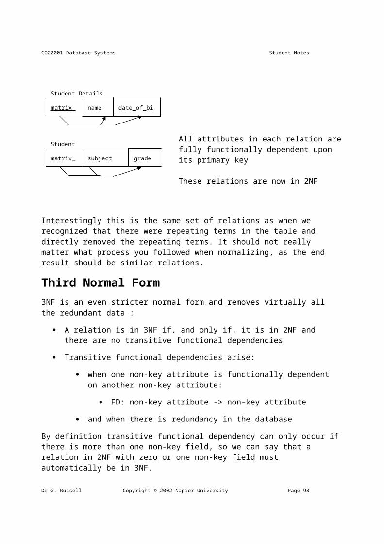
08/05/23 15:04 CO22001 Database Systems
JOIN -> |x| (bow-tie)
UNION -> (cup)
INTERSECTION -> (cap)
DIFFERENCE -> - (minus)
RENAME -> (rho)
Usage The symbolic operators are used as with the verbal ones. So, to find all employees in department 1:
SELECTdepno = 1(employee) becomes depno = 1(employee)
Conditions can be combined together using ^ (AND) and v (OR). For example, all employees in department 1 called `Smith':
SELECTdepno = 1 ^ surname = `Smith'(employee) becomes depno = 1 ^ surname = `Smith'(employee)
The use of the symbolic notation can lend itself to brevity. Even better, when the JOIN is a natural join, the JOIN condition may be omitted from |x|. The earlier example resulted in:
PROJECTdname (department JOINdepno = depno ( PROJECTdepno (employee JOINempno = empno ( PROJECTempno (empcourse JOINcourseno = courseno ( PROJECTcourseno (SELECTcname = `Further Accounting' course)))))))
becomes
dname (department |x| ( depno (employee |x| ( empno (empcourse |x| ( courseno (cname = `Further Accounting' course) ))))))
Rename Operator The rename operator returns an existing relation under a new name. A(B) is the relation B with its name changed to A. For example, find the employees in the same Department as employee 3.
emp2.surname,emp2.forenames ( employee.empno = 3 ^ employee.depno = emp2.depno ( employee (emp2employee) ) )
Page 94 Copyright © 2001 Napier University +44 141 455 2754

CO22001 Database Systems Student Notes
Derivable Operators Fundamental operators:, , , , -,
Derivable operators: |x|,
A
B<=> A - (A - B)
A B
A B
A B
Equivalence A|x|cB <=> a1,a2,...aN(c(A B))
where c is the join condition (eg A.a1 = B.a1),
and a1,a2,...aN are all the attributes of A and B without repetition.
c is called the join-condition, and is usually the comparison of primary and foreign key. Where there are N tables, there are usually N-1 join-conditions. In the case of a natural join, the conditions can be missed out, but otherwise missing out conditions results in a cartesian product (a common mistake to make).
Equivalences The same relational algebraic expression can be written in many different ways. The order in which tuples appear in relations is never significant.
A B <=> B A
A B <=> B A
A B <=> B A
(A - B) is not the same as (B - A)
c1 (c2(A)) <=> c2 (c1(A)) <=> c1 ^ c2(A)
a1(A) <=> a1(a1,etc(A))where etc represents any other attributes of A.
Dr G. Russell Copyright © 2002 Napier University Page 95
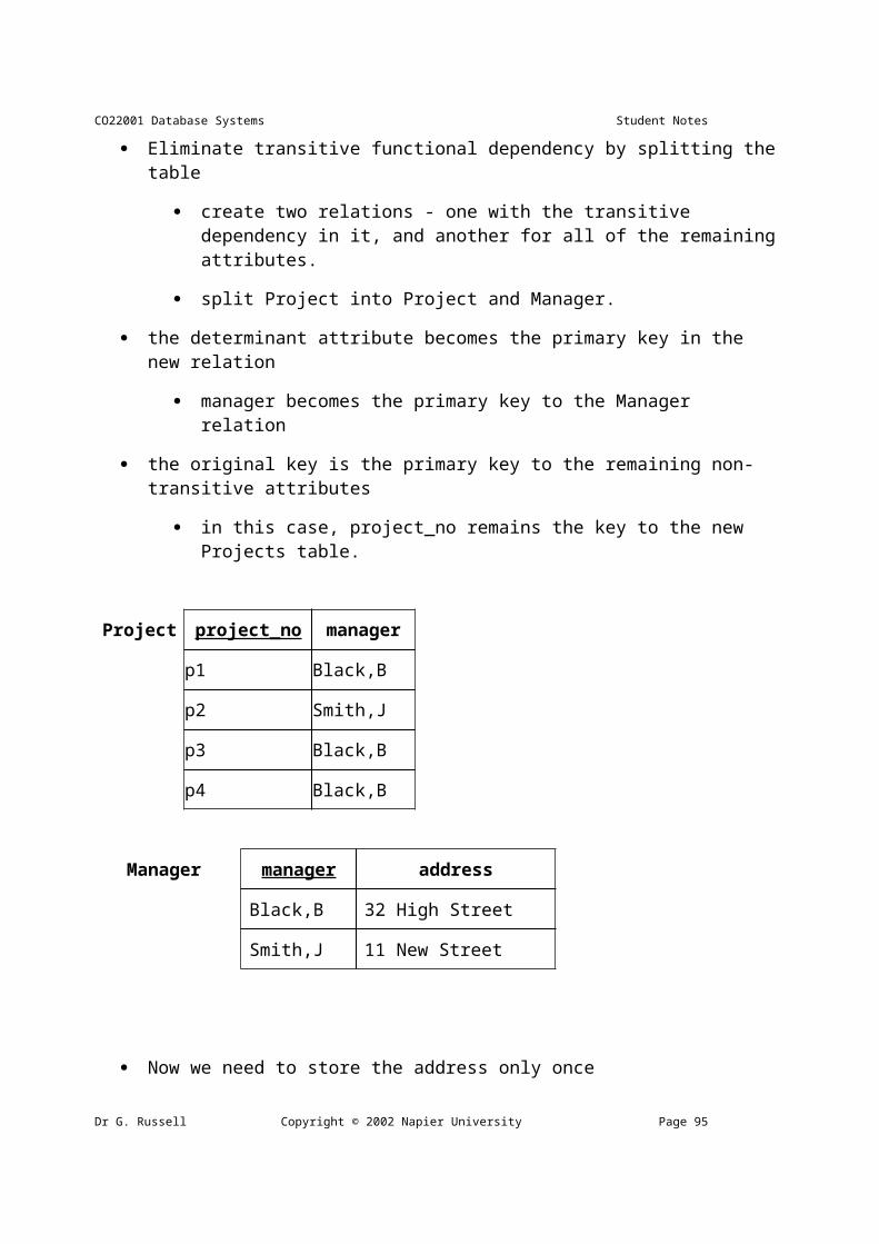
08/05/23 15:04 CO22001 Database Systems
many other equivalences exist.
While equivalent expressions always give the same result, some may be much easier to evaluate that others.
When any query is submitted to the DBMS, its query optimiser tries to find the most efficient equivalent expression before evaluating it.
Comparing RA and SQL Relational algebra:
is closed (the result of every expression is a relation)
has a rigorous foundation
has simple semantics
is used for reasoning, query optimisation, etc.
SQL:
is a superset of relational algebra
has convenient formatting features, etc.
provides aggregate functions
has complicated semantics
is an end-user language.
Comparing RA and SQL Any relational language as powerful as relational algebra is called relationally complete.
A relationally complete language can perform all basic, meaningful operations on relations.
Since SQL is a superset of relational algebra, it is also relationally complete.
Page 96 Copyright © 2001 Napier University +44 141 455 2754

CO22001 Database Systems Student Notes
Unit 4.1 - TransactionsUnit 4.1 - Concurrency using Transactions The goal in a `concurrent' DBMS is to allow multiple users to access the database simultaneously without interfering with each other.
A problem with multiple users using the DBMS is that it may be possible for two users to try and change data in the database simultaneously. If this type of action is not carefully controlled, inconsistencies are possible.
To control data access, we first need a concept to allow us to encapsulate database accesses. Such encapsulation is called a `Transaction'.
Transactions Transaction (ACID)
unit of logical work and recovery
atomicity (for integrity)
consistency preservation
isolation
durability
Available in SQL
Some applications require nested or long transactions
After work is performed in a transaction, two outcomes are possible:
Commit - Any changes made during the transaction by this transaction are committed to the database.
Abort - All the changes made during the transaction by this transaction are not made to the database. The result of this is as if the transaction was never started.
Transaction Schedules A transaction schedule is a tabular representation of how a set of transactions were executed over time. This is useful when examining problem scenarios. Within the diagrams various nomenclatures are used:
READ(a) - This is a read action on an attribute or data item called `a'.
Dr G. Russell Copyright © 2002 Napier University Page 97
08/05/23 15:04 CO22001 Database Systems
WRITE(a) - This is a write action on an attribute or data item called `a'.
WRITE(a[x]) - This is a write action on an attribute or data item called `a', where the value `x' is written into `a'.
tn (e.g. t1,t2,t10) - This indicates the time at which something occurred. The units are not important, but tn always occurs before tn+1.
Consider transaction A, which loads in a bank account balance X (initially 20) and adds 10 pounds to it. Such a schedule would look like this:
Time Transaction A
t1 TOTAL:=READ(X)
t2 TOTAL:=TOTAL+10
t3 WRITE(X[30])
Now consider that, at the same time as transaction A runs, transaction B runs. Transaction B gives all accounts a 10% increase. Will X be 32 or 33?
Time Transaction A Transaction B
t1 TOTAL:=READ(X)
t2 TOTAL:=READ(X)
t3 TOTAL:=TOTAL+10
t4 WRITE(X[30])
t5 TOTAL:=TOTAL*110%
t6 WRITE(X[22])
Whoops... X is 22! Depending on the interleaving, X can also be 32, 33, or 30. Lets classify erroneous scenarios.
Page 98 Copyright © 2001 Napier University +44 141 455 2754

CO22001 Database Systems Student Notes
Lost Update scenario. Time Transaction A Transaction B
t1 READ(R)
t2 READ(R)
t3 WRITE(R)
t4 WRITE(R)
Transaction A's update is lost at t4, because Transaction B overwrites it. B missed A's update at t3 as it got the value of R at t2.
Uncommitted Dependency
Time Transaction A Transaction B
t1 WRITE(R)
t2 READ(R)
t3 ABORT
Transaction A is allowed to READ (or WRITE) item R which has been updated by another transaction but not committed (and in this case ABORTed).
Dr G. Russell Copyright © 2002 Napier University Page 99
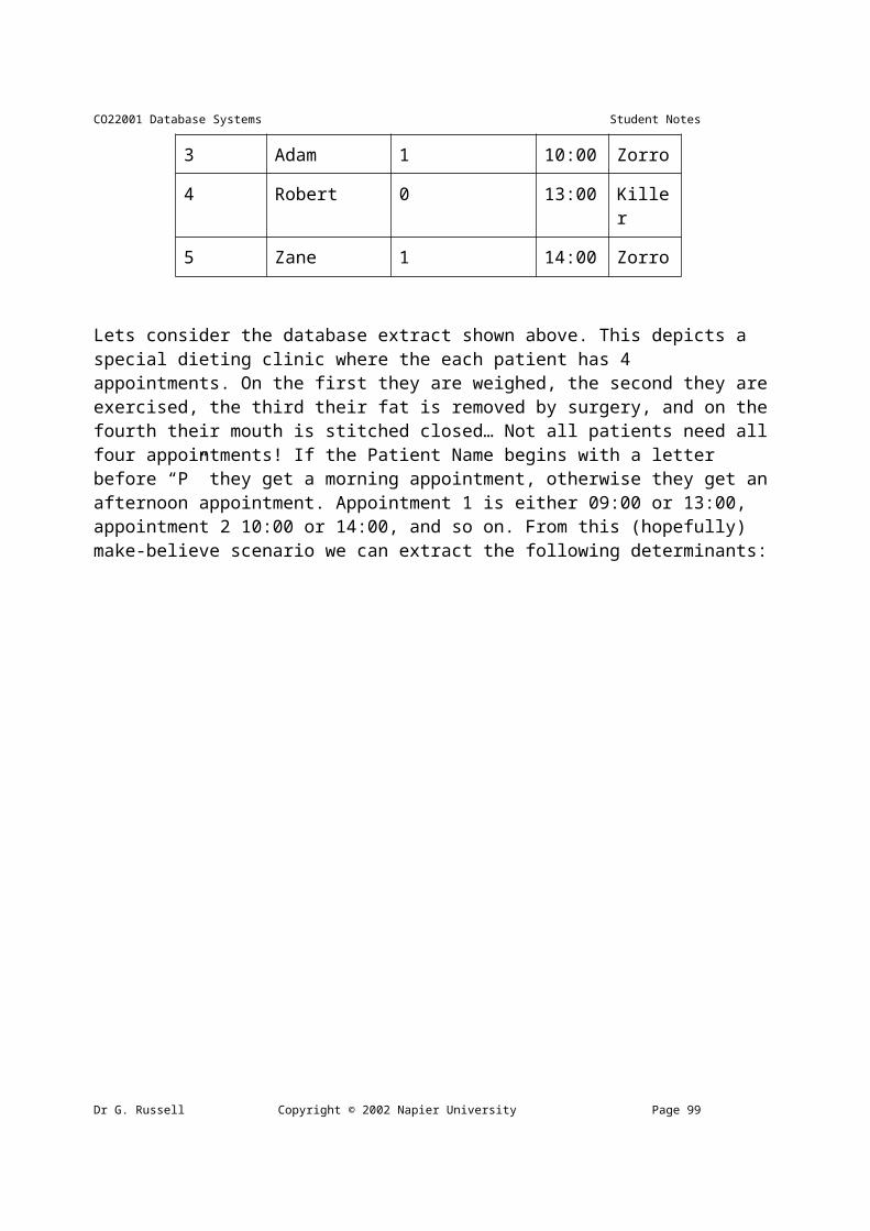
08/05/23 15:04 CO22001 Database Systems
Inconsistency Time X Y Z Transaction A Transaction B
Action SUM
t1 40 50 30 SUM:=READ(X) 40
t2 40 50 30 SUM+=READ(Y) 90
t3 40 50 30 READ(Z)
t4 40 50 20 WRITE(Z[20])
t5 40 50 20 READ(X)
t6 50 50 20 WRITE(X[50])
t7 50 50 20 COMMIT
t7 50 50 20 SUM+=READ(Z) 110
SUM should have been 120...
Serialisability A `schedule' is the actual execution sequence of two or more concurrent
transactions.
A schedule of two transactions T1 and T2 is `serialisable' if and only if executing this schedule has the same effect as either T1;T2 or T2;T1.
Precedence Graph In order to know that a particular transaction schedule can be serialized, we can draw a precedence graph. This is a graph of nodes and vertices, where the nodes are the transaction names and the vertices are attribute collisions. To draw one;
The schedule is said to be serialised if and only if there are no cycles in the resulting diagram.
Precedence Graph : Method To draw one;
1. Draw a node for each transaction in the schedule
2. Where transaction A writes to an attribute which transaction B has read from, draw an line pointing from B to A.
Page 100 Copyright © 2001 Napier University +44 141 455 2754

CO22001 Database Systems Student Notes
3. Where transaction A writes to an attribute which transaction B has written to, draw a line pointing from B to A.
4. Where transaction A reads from an attribute which transaction B has written to, draw a line pointing from B to A.
Example 1 Consider the following schedule:
T1 time T2
read(A) t1
read(B) t2
t3 read(A)
t4 read(B)
t5
write(B) t6
t7 write(B)
Example 2 Consider the following schedule:
T1 time T2 T3
read(A) t1
read(B) t2
t3 read(A)
t4 read(B)
write(C) t5
t6 write(A)
write(B) t7
t8 write(C)
Dr G. Russell Copyright © 2002 Napier University Page 101
T1 T2
T3 T2
T1B
C
A
A
B
B
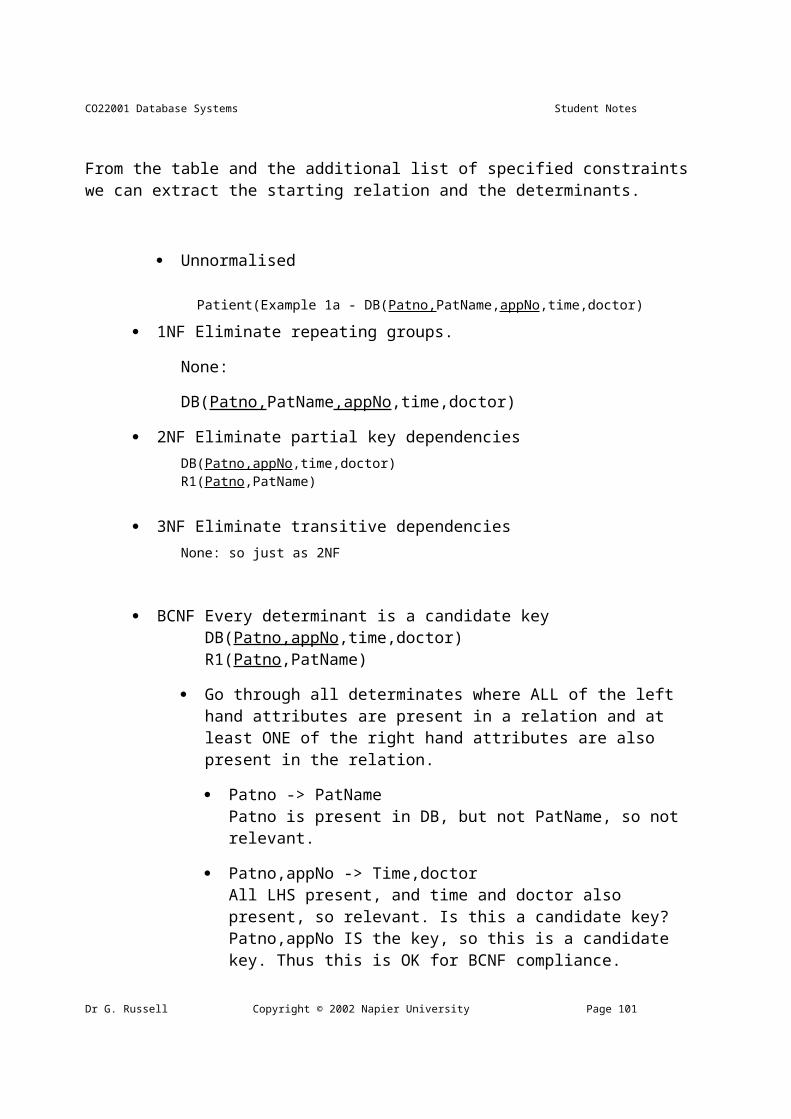
08/05/23 15:04 CO22001 Database Systems
Unit 4.2 - ConcurrencyUnit 4.2 - ConcurrencyLocking
A solution to enforcing serialisability?
read (shareable) lock
write (exclusive) lock
coarse granularity
easier processing
less concurrency
fine granularity
more processing
higher concurrency
Many systems use locking mechanisms for concurrency control. When a transaction needs an assurance that some object will not change in some unpredictable manner, it acquires a lock on that object.
A transaction holding a read lock is permitted to read an object but not to change it.
More than one transaction can hold a read lock for the same object.
Usually, only one transaction may hold a write lock on an object.
On a transaction schedule, we use `S' to indicate a shared lock, and `X' for an exclusive write lock.
Page 102 Copyright © 2001 Napier University +44 141 455 2754
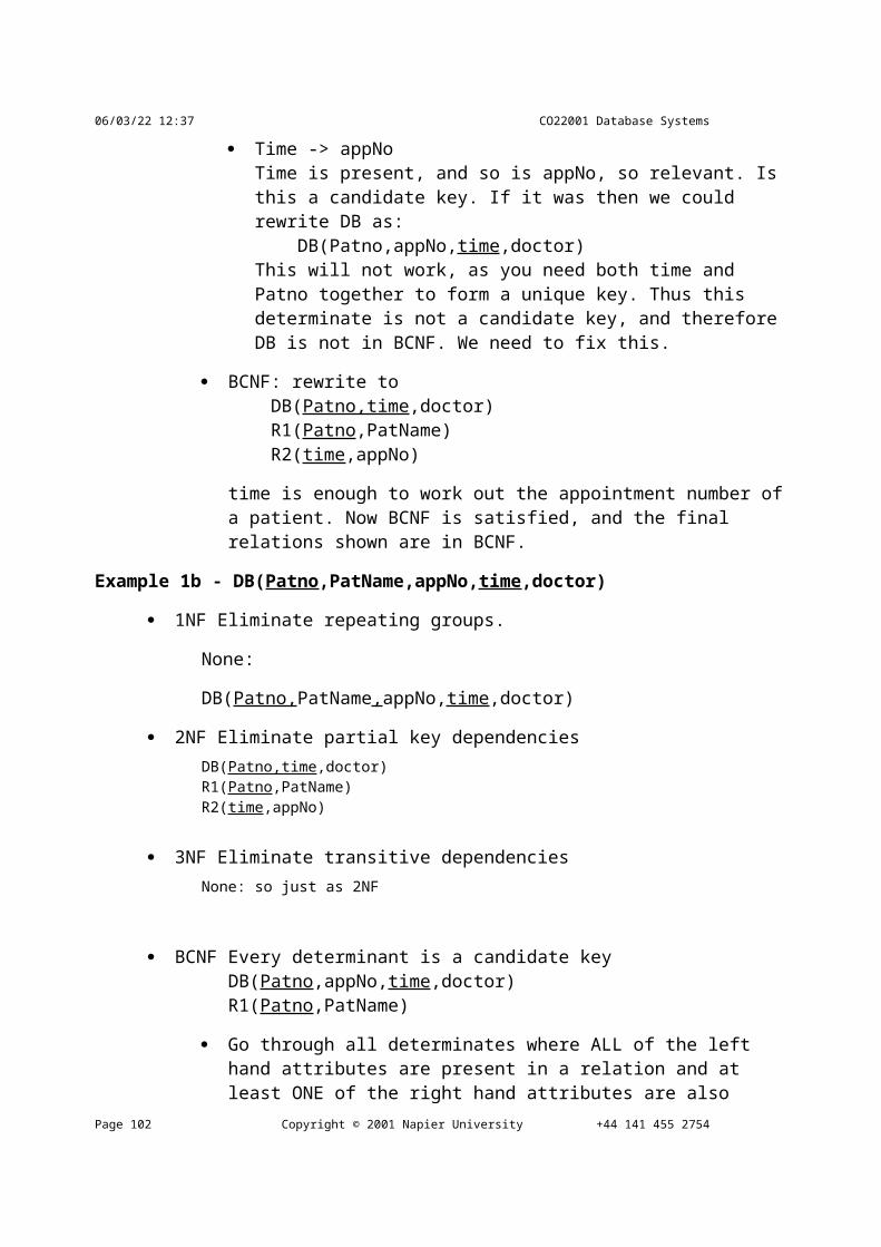
CO22001 Database Systems Student Notes
Locking - Uncommitted Dependency Locking solves the uncommitted dependency problem.
Time Transaction A Transaction B Lock on R
t1 WRITE(R) - = X
t2 READ R (WAIT) X
t3 ...wait... ABORT X = -
t4 READ R (CONT) - = S
Deadlock Deadlock can arise when locks are used, and causes all related transactions to WAIT forever...
time Transaction A Transaction B Lock State
X Y
t1 WRITE(X) - = X -
t2 WRITE(Y) X - = X
t3 READ(Y) (WAIT) X X
t3 ...WAIT... READ(X) (WAIT) X X
t3 ...WAIT... ...WAIT... X X
The `lost update' senario results in deadlock with locks. So does the `inconsistency' scenario.
Dr G. Russell Copyright © 2002 Napier University Page 103
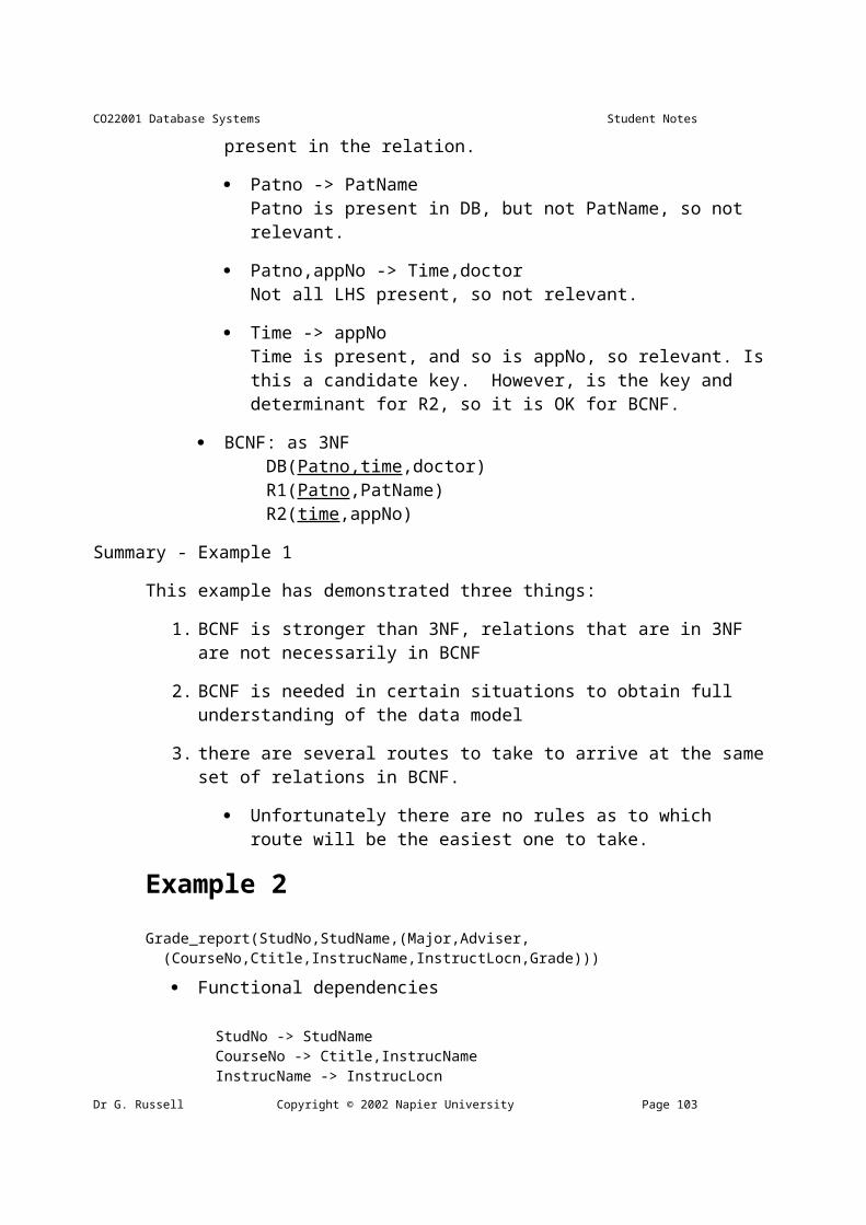
08/05/23 15:04 CO22001 Database Systems
time Transaction A Transaction B Lock R
t1 READ(R) - = S
t2 READ(R) S = S
t3 WRITE(R) (WAIT) S
t3 ...wait... WRITE(R) (WAIT) S
t3 ...wait... ...wait... S
Deadlock Handling Deadlock avoidance
pre-claim strategy used in operating systems
not effective in database environments.
Deadlock detection
whenever a lock requests a wait, or on some perodic basis.
if a transaction is blocked due to another transaction, make sure that that transaction is not blocked on the first transaction, either directly or indirectly via another transaction.
Page 104 Copyright © 2001 Napier University +44 141 455 2754
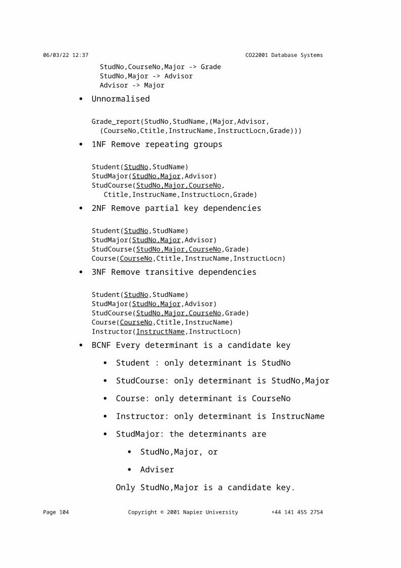
CO22001 Database Systems Student Notes
Deadlock Resolution If a set of transactions is considered to be deadlocked:
1. choose a victim (e.g. the shortest-lived transaction)
2. rollback `victim' transaction and restart it.
The rollback terminates the transaction, undoing all its updates and releasing all of its locks.
A message is passed to the victim and depending on the system the transaction may or may not be started again automatically.
Two-Phase Locking The presence of locks does not guarantee serialisability. If a transaction is allowed to release locks before the transaction has completed, and is also allowed to acquire more (or even the same) locks later then the benifit or locking is lost.
If all transactions obey the `two-phase locking protocol', then all possible interleaved executions are guarenteed serialisable.
The two-phase locking protocol:
Before operating on any item, a transaction must acquire at least a shared lock on that item. Thus no item can be accessed without first obtaining the correct lock.
After releasing a lock, a transaction must never go on to acquire any more locks.
The technical names for the two phases of the locking protocol are the `lock-acquisition phase' and the `lock-release phase'.
Other Database Consistency Methods Two-phase locking is not the only approach to enforcing database consistency. Another method used in some DMBS is timestamping. With timestamping, there are no locks to prevent transactions seeing uncommitted changes, and all physical updates are deferred to commit time.
locking synchronises the interleaved execution of a set of transactions in such a way that it is equivalent to some serial execution of those transactions.
timestamping synchronises that interleaved execution in such a way that it is equivalent to a particular serial order - the order of the timestamps.
Dr G. Russell Copyright © 2002 Napier University Page 105
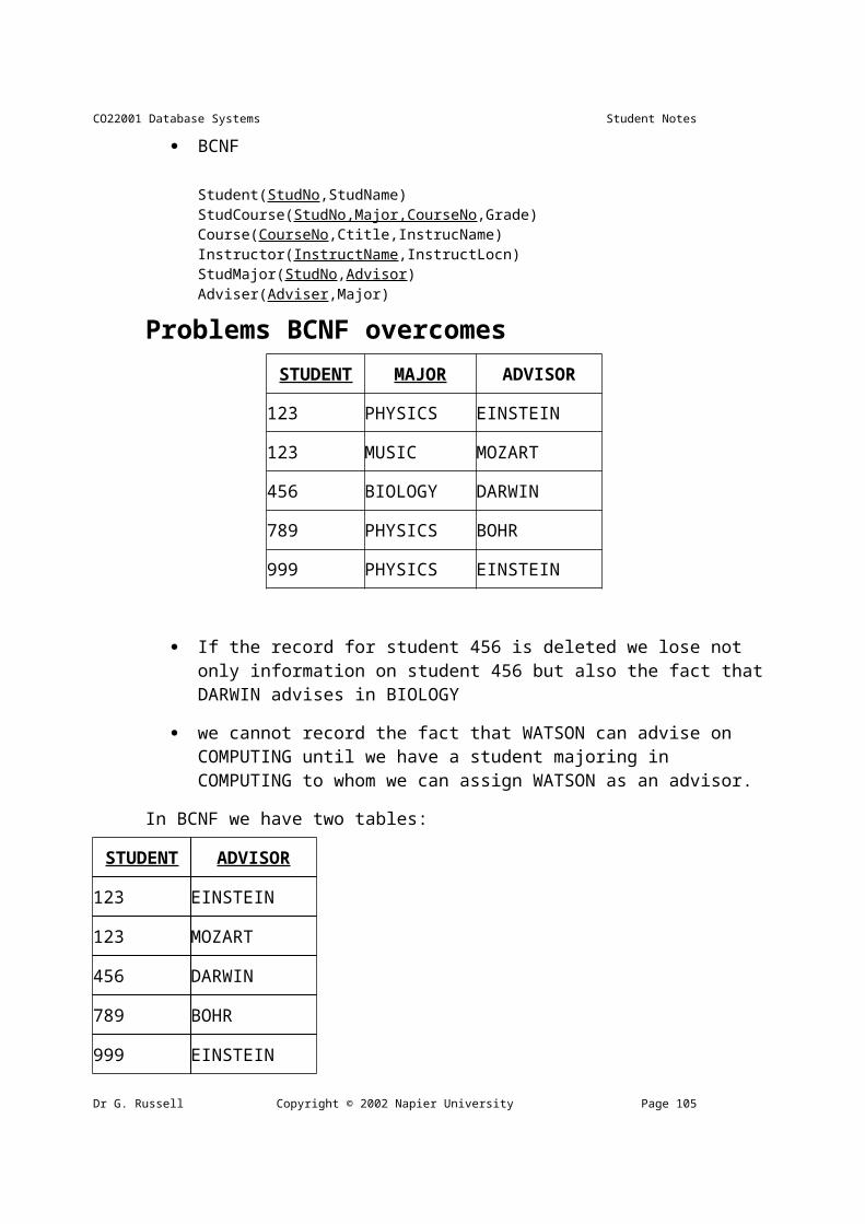
08/05/23 15:04 CO22001 Database Systems
Timestamping rules The following rules are checked when transaction T attempts to change a data item. If the rule indicates ABORT, then transaction T is rolled back and aborted (and perhaps restarted).
If T attempts to read a data item which has already been written to by a younger transaction then ABORT T.
If T attempts to write a data item which has been seen or written to by a younger transaction then ABORT T.
If transaction T aborts, then all other transactions which have seen a data item written to by T must also abort. In addition, other aborting transactions can cause further aborts on other transactions. This is a `cascading rollback'.
Page 106 Copyright © 2001 Napier University +44 141 455 2754

CO22001 Database Systems Student Notes
Unit 4.3 - Storage StructuresUnit 4.3 – Storage Structures
The Physical Store Storage Medium Transfer Rate Capacity Seek Time
Main Memory 800 MB/s 100 MB Instant
Hard Drive 10 MB/s 10 GB 10 ms
CD-ROM Drive 5 MB/s 0.6 GB 100 ms
Floppy Drive 2 MB/s 1.44 MB 300 ms
Tape Drive 1 MB/s 20 GB 30 s
Why not all Main Memory? The performance of main memory is the greatest of all storage methods, but it is also the most expensive per MB.
All the other types of storage are `persistent'. A persistent store keeps the data stored on it even when the power is switched off.
Only main memory can be directly accessed by the programmer. Data held using other methods must be loaded into main memory before being accessed, and must be transferred back to storage from main memory in order to save the changes.
We tend to refer to storage methods which are not main memory as `secondary storage'.
Secondary Storage - Blocks All storage devices have a block size. Block size is the minimum amount which can be read or written to on a storage device. Main memory can have a block size of 1-8 bytes, depending on the processor being used. Secondary storage blocks are usually much bigger.
Hard Drive disk blocks are usually 4 KBytes in size.
For efficiency, multiple contiguous blocks can be be requested.
On average, to access a block you first have to request it, wait the seek time, and then wait the transfer time of the blocks requested.
Dr G. Russell Copyright © 2002 Napier University Page 107

08/05/23 15:04 CO22001 Database Systems
Remember, you cannot read or write data smaller than a single block.
Hard Drives The most common secondary storage medium for DBMS is the hard drive.
Data on a hard-drive is often arranged into files by the Operating System.
the DBMS holds the database within one or more files.
The data is arranged within a file in blocks, and the position of a block within a file is controlled by the DBMS.
Files are stored on the disk in blocks, but the placement of a file block on the disk is controlled by the O/S (although the DBMS may be allowed to `hint' to the O/S concerning disk block placement strategies).
File blocks and disk blocks are not necessarily equal in size.
DBMS Data Items Data from the DBMS is split into records.
a record is a logical collection of data items
a file is a collection of records.
one or more records may map onto a single or multiple file blocks.
a single record may map onto multiple file blocks.
Comparing terminology...
Relational SQL Physical Storage
Relation Table File
Tuple Row Record
Attribute Column Data Item/Field
Domain Type Data Type
File Organisations Serial (or unordered, or heap) - records are written to secondary storage in the
order in which they are created.
Sequential (or sorted, or ordered) - records are written to secondary storage in the sorted order of a key (one or more data items) from each record.
Page 108 Copyright © 2001 Napier University +44 141 455 2754

CO22001 Database Systems Student Notes
Hash - A `hash' function is applied to each record key, which returns a number used to indicate the position of the record in the file. The hash function must be used for both reading and writing.
Indexed - the location in secondary storage of some (partial index) or all (full index) records is noted in an index.
Storage Scenario To better explain each of these file organisations we will create 4 records and place them in secondary storage. The records are created by a security guard, and records who passes his desk in the morning and at what time they pass.
The records therefore each have three data items; `name', `time', and `id number'. Only four people arrive for work:
1. name=`Russell' at time=`0800' with id_number=`004'.
2. name=`Greg' at time=`0810' with id_number=`007'.
3. name=`Jon' at time=`0840' with id_number=`002'.
4. name=`Cumming' at time=`0940' with id_number=`003'.
Serial Organisation
1 2 3 4
Russell0800004
Greg Jon Cumming0810 0840 0940007 002 003
Writing - the data is written at the end of the previous record.
Reading -
reading records in the order they were written is a cheap operation.
Trying to find a particular record means you have to read each record in turn until you locate it. This is expensive.
Deleting - Deleting data in such an structure usually means marking the data as deleted (thus not actually removing it) which is cheap but wasteful or rewriting the whole file to overwrite the deleted record (space-efficient but expensive).
Sequential Organisation Russell0800004
Jon0840002
Cumming0940003
Greg0810007
3 41 2Dr G. Russell Copyright © 2002 Napier University Page 109

08/05/23 15:04 CO22001 Database Systems
Writing - records are in `id number' order, thus new records may need to be inserted into the store needing a complete file copy (expensive).
Deleting - as with serial, either leave holes or perform make file copies.
Reading -
reading records in `id number' order is cheap.
the ability to chose sort order makes this more useful than serial.
`binary search' could be used. Goto middle of file - if record key greater than that wanted search the low half, else search the high half, until the record is found. (average accesses to find something is log2no_of_records.)
Hash Organisation
Greg0810007
Russell0800004
Jon0840002
Cumming0940003
3 41 2
Key (id number) Key MOD 6
Writing - Initially the file has 6 spaces (n MOD 6 can be 0-5). To write, calculate the hash and write the record in that location (cheap).
Deleting - leave holes by marking the record deleted (wasteful of space but cheap to process).
Reading -
reading records an order is expensive.
finding a particular record from a key is cheap and easy.
If two records can result in the same hash number, then a strategy must be found to solve this problem (which will incur overheads).
Indexed Sequential Access Method The Indexed Sequential Access Method (ISAM) is frequently used for partial indexes.
there may be several levels of indexes, commonly 3
each index-entry is equal to the highest key of the records or indices it points to.
the records of the file are effectively sorted and broken down into small groups of data records.
Page 110 Copyright © 2001 Napier University +44 141 455 2754
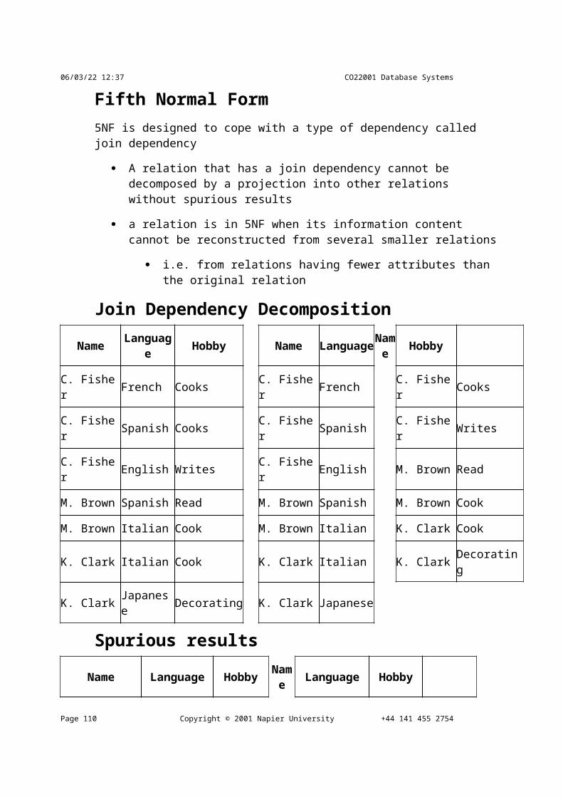
CO22001 Database Systems Student Notes
the indices are built when the data is first loaded as sorted records.
the index is static, and does not change as records are inserted and deleted
insertion and deletion adds to one of the small groups of data records. As the number in each group changes, the performance may deteriorate.
ISAM Example
B+ Tree Index With B+ tree, a full index is maintained, allowing the ordering of the records in the file to be independent of the index. This allows multiple B+ tree indices to be kept for the same set of data records.
the lowest level in the index has one entry for each data record.
the index is created dynamically as data is added to the file.
as data is added the index is expanded such that each record requires the same number of index levels to reach it (thus the tree stays `balanced').
the records can be accessed via an index or sequentially.
Each index node in a B+ Tree can hold a certain number of keys. The number of keys is often referred to as the `order'. Unfortunately, `Order 2' and `Order 1' are frequently confused in the database literature. For the purposes of our coursework and exam, `Order 2' means that there can be a maximum of 2 keys per index node. In this module, we only ever consider order 2 B+ trees.
Dr G. Russell Copyright © 2002 Napier University Page 111

08/05/23 15:04 CO22001 Database Systems
B+ Tree Example
90 60 55 70 65 30 10 69
10 30 55 60 65 69 70 90
30 55 69 70
60
Building a B+ Tree Only nodes at the bottom of the tree point to records, and all other nodes point to
other nodes. Nodes which point to records are called leaf nodes.
If a node is empty the data is added on the left.
If a node has one entry, then the left takes the smallest valued key and the right
takes the biggest. 6030
If a node is full and is a leaf node, classify the keys L (lowest), M (middle value) and H (highest), and split the node.
L M H
M
If a node is full and is not a leaf node, classify the keys L (lowest), M (middle value) and H (highest), and split the node.
L H
M
Page 112 Copyright © 2001 Napier University +44 141 455 2754
CO22001 Database Systems Student Notes
B+ Tree Build Example 60
55 60 70 90
60
55 60 907065
70
90 60 90
60
55 60 90
Add 90 Add 60 Add 55 Add 70
Add 65 Add 30
90706555 6030
70
60
55
90706560
70
60
55
30 5510
30
Add 10
6560
60
55
30 5510
30
Add 69
7069
907069
Index Structure and Access The top level of an index is usually held in memory. It is read once from disk at
the start of queries.
Each index entry points to either another level of the index, a data record, or a block of data records.
The top level of the index is searched to find the range within which the desired record lies.
The appropriate part of the next level is read into memory from disc and searched.
This continues until the required data is found.
The use of indices reduce the amount of file which has to be searched.
Dr G. Russell Copyright © 2002 Napier University Page 113

08/05/23 15:04 CO22001 Database Systems
Costing Index and File Access The major cost of accessing an index is associated with reading in each of the
intermediate levels of the index from a disk (milliseconds).
Searching the index once it is in memory is comparatively inexpensive (microseconds).
The major cost of accessing data records involves waiting for the media to recover the required blocks (milliseconds).
Some indexes mix the index blocks with the data blocks, which means that disk accesses can be saved because the final level of the index is read into memory with the associated data records.
Use of Indexes A DBMS may use different file organisations for its own purposes.
A DBMS user is generally given little choice of file type.
A B+ Tree is likely to be used wherever an index is needed.
Indexes are generated:
(Probably) for fields specified with `PRIMARY KEY' or `UNIQUE' constraints in a CREATE TABLE statement.
For fields specified in SQL statements such as CREATE [UNIQUE] INDEX indexname ON tablename (col [,col]...);
Primary Indexes have unique keys.
Secondary Indexes may have duplicates.
An index on a column which is used in an SQL `WHERE' predicate is likely to speed up an enquiry.
this is particularly so when `=' is involved (equijoin)
no improvement will occur with `IS [NOT] NULL' statements
an index is best used on a column which widely varying data.
indexing and column of Y/N values might slow down enquiries.
an index on telephone numbers might be very good but an index on area code might be a poor performer.
Multicolumn index can be used, and the column which has the biggest range of values or is the most frequently accessed should be listed first.
Page 114 Copyright © 2001 Napier University +44 141 455 2754
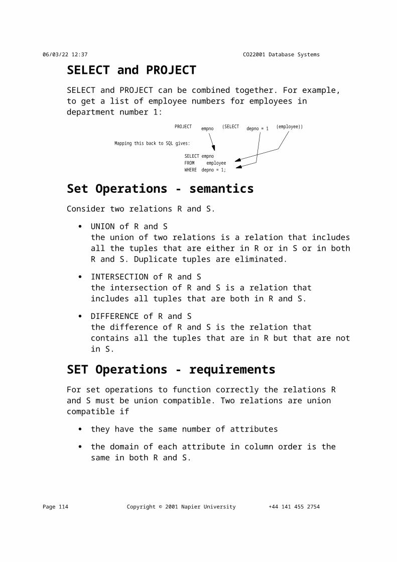
CO22001 Database Systems Student Notes
Avoid indexing small relations, frequently updated columns, or those with long strings.
There may be several indexes on each table. Note that partial indexing normally supports only one index per table.
Reading or updating a particular record should be fast.
Inserting records should be reasonably fast. However, each index has to be updated too, so increasing the indexes makes this slower.
Deletion may be slow.
particularly when indexes have to be updated.
deletion may be fast if records are simply flagged as `deleted'.
Unit 4.4 - RecoveryUnit 4.4 - Recovery A database might be left in an inconsistent state when:
deadlock has occurred.
a transaction aborts after updating the database.
software or hardware errors.
incorrect updates have been applied to the database.
If the database is in an inconsistent state, it is necessary to recover to a consistent state. The basis of recovery is to have backups of the data in the database.
Recovery: the dump The simplest backup technique is `the Dump'.
entire contents of the database is backed up to an auxiliary store.
must be performed when the state of the database is consistent - therefore no transactions which modify the database can be running
dumping can take a long time to perform
you need to store the data in the database twice.
as dumping is expensive, it probably cannot be performed as often as one would like.
a cut-down version can be used to take `snapshots' of the most volatile areas.
Dr G. Russell Copyright © 2002 Napier University Page 115

08/05/23 15:04 CO22001 Database Systems
Recovery: the transaction log A technique often used to perform recovery is the transaction log or journal.
records information about the progress of transactions in a log since the last consistent state.
the database therefore knows the state of the database before and after each transaction.
every so often database is returned to a consistent state and the log may be truncated to remove committed transactions.
when the database is returned to a consistent state the process is often referred to as `checkpointing'.
Deferred Update Deferred update, or NO-UNDO/REDO, is an algorithm to support ABORT and machine failure scenarios.
While a transaction runs, no changes made by that transaction are recorded in the database.
On a commit:
1. The new data is recorded in a log file and flushed to disk
2. The new data is then recorded in the database itself.
On an abort, do nothing (the database has not been changed).
On a system restart after a failure, REDO the log.
Example Consider the following transaction T1
Transaction T1
read(A)
write(B[10])
write(C[20])
Commit
Using deferred update, the process is:
Time Action Data
Page 116 Copyright © 2001 Napier University +44 141 455 2754

CO22001 Database Systems Student Notes
t1 START -
t2 read(A) -
t3 write(B) B = 10
t4 write(C) C = 20
t5 COMMIT -
Before After
Disk B=6 B=10
A=5 C=2 A=5 C=20
If the DMBS fails and is restarted:
1. The disks are physically or logically damaged then recovery from the log is impossible and instead a restore from a dump is needed.
2. If the disks are OK then the database consistency must be maintained. Writes to the disk which was in progress at the time of the failure may have only been partially done.
3. Parse the log file, and where a transaction has been ended with `COMMIT' apply the data part of the log to the database.
4. If a log entry for a transaction ends with anything other than COMMIT, do nothing for that transaction.
5. flush the data to the disk, and then truncate the log to zero.
6. the process or reapplying transaction from the log is sometimes referred to as `rollforward'.
Immediate Update Immediate update, or UNDO/REDO, is another algorithm to support ABORT and machine failure scenarios.
While a transaction runs, changes made by that transaction can be written to the database at any time. However, the original and the new data being written must both be stored in the log BEFORE storing it on the database disk.
On a commit:
1. All the updates which has not yet been recorded on the disk is first stored
Dr G. Russell Copyright © 2002 Napier University Page 117

08/05/23 15:04 CO22001 Database Systems
in the log file and then flushed to disk.
2. The new data is then recorded in the database itself.
On an abort, REDO all the changes which that transaction has made to the database disk using the log entries.
On a system restart after a failure, REDO committed changes from log.
Example Using immediate update, and the transaction T1 again, the process is:
Time Action Old Data New Data
t1 START - -
t2 read(A) - -
t3 write(B) B == 6 B = 10
t4 write(C) C == 2 C = 20
t5 COMMIT - -
Page 118 Copyright © 2001 Napier University +44 141 455 2754
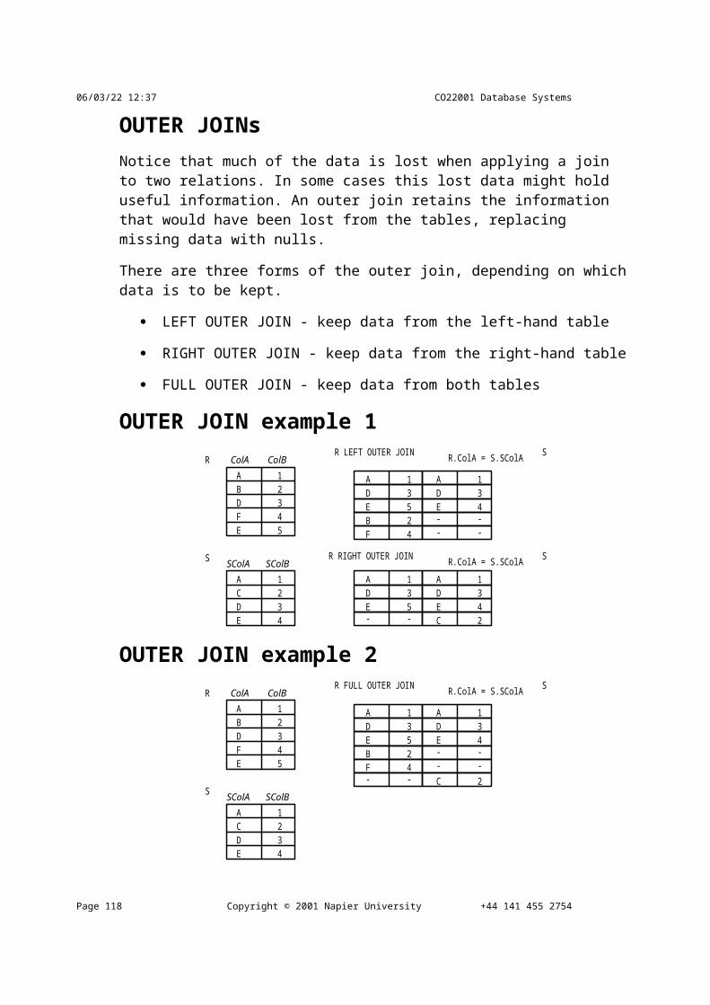
CO22001 Database Systems Student Notes
Before During After
Disk B=6 B=1
0 B=10
A=5 C=2 A=5 C=2 A=5 C=20
If the DMBS fails and is restarted:
1. The disks are physically or logically damaged then recovery from the log is impossible and instead a restore from a dump is needed.
2. If the disks are OK then the database consistency must be maintained. Writes to the disk which was in progress at the time of the failure may have only been partially done.
3. Parse the log file, and where a transaction has been ended with `COMMIT' apply the `new data' part of the log to the database.
4. If a log entry for a transaction ends with anything other than COMMIT, apply the `old data' part of the log to the database.
5. flush the data to the disk, and then truncate the log to zero.
Rollback The process of undoing changes done to the disk under immediate update is frequently referred to as rollback.
Where the DBMS does not prevent one transaction from reading uncommitted modifications (a `dirty read') of another transaction (i.e. the uncommitted dependency problem) then aborting the first transaction also means aborting all the transactions which have performed these dirty reads.
as a transaction is aborted, it can therefore cause aborts in other dirty reader transactions, which in turn can cause other aborts in other dirty reader transaction. This is referred to as `cascade rollback'.
Dr G. Russell Copyright © 2002 Napier University Page 119
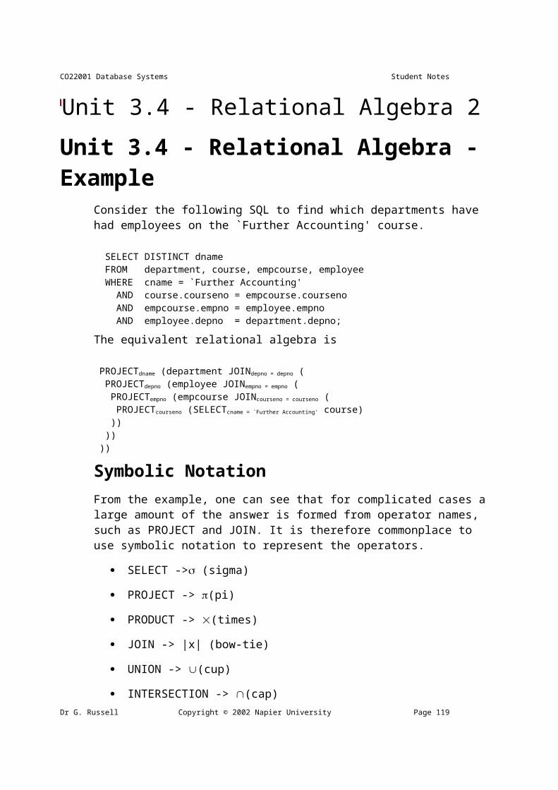
08/05/23 15:04 CO22001 Database Systems
Unit 5.1 - Embedded SQLUnit 5.1 - Embedded SQL Interactive SQL So far in the module we have considered only the SQL queries which you can type in at the SQL prompt. We refer to this as `interactive' SQL. This is a good way to learn SQL. Interactive SQL also allows the database designer to set up the database structure (tables and so forth), making small queries or one-off queries, and for testing out ways to extract data from the database.
SQL itself is a `non-procedural' language. There are no good ways to build up complex queries, and reuse of queries is complicated. It is good at specifying WHAT is required of the database, but its control of how the data is manipulated to solve real-world problem specifications is weak.
Interactive SQL it is not good for more sophisticated applications for which a programming language with links to SQL might be better. To this end the idea of EMBEDDED SQL was produced.
Embedded SQL SQL can be embedded within procedural programming languages. These language (sometimes referred to as 3GLs) include C/C++, Cobol, Fortran, and Ada. Thus the embedded SQL provides the 3GL with a way to manipulate a database, supporting:
highly customized applications
background applications running without user intervention
database manipulation which exceeds the abilities of simple SQL
applications linking to Oracle packages, e.g. forms and reports
applications which need customized window interfaces
SQL Precompiler A precompiler is used to translate SQL statements embedded in a host language into DBMS library calls which can be implemented in the host language.
Page 120 Copyright © 2001 Napier University +44 141 455 2754
CO22001 Database Systems Student Notes
Editor
Precompiler
Linker
Compiler
host program + embedded SQL
executable program
object (binary) program
host program + translated SQL
DBMS and other libraries
Sharing Variables Variables to be shared between the embedded SQL code and the 3GL have to be specified in the program.
EXEC SQL begin declare section; varchar userid[10],password[10],cname[15]; int cno;EXEC SQL end declare section;
We also should declare a link to the DBMS so that database status information can be accessed.
EXEC SQL include sqlca;
This allows access to a structure sqlca, of which the most common element sqlca.sqlcode has the value 0 (operation OK), >0 (no data found), and <0 (an error).
Connecting to the DBMS Before operations can be performed on the database, a valid connection has to be established.
EXEC SQL connect :userid identified by :password;
In all SQL statements, variables with the `:' prefix refer to shared host variables, as opposed to database variables (e.g. row or column identifiers).
This assumes that userid and password have been properly declared and initialised.
When the program is finished using the DBMS, it should disconnect using:
EXEC SQL commit release;
Queries producing a single row A single piece of data (or row) can be queried from the database so that the result is accessible from the host program.
EXEC SQL SELECT custname
Dr G. Russell Copyright © 2002 Napier University Page 121

08/05/23 15:04 CO22001 Database Systems
INTO :cname FROM customers WHERE cno = :cno;
Thus the custname with the unique identifier :cno is stored in :cname.
However, a selection query may generate many rows, and a way is needed for the host program to access results one row at a time.
SELECT with a single result
Cursors - SELECT many rows A cursor provides a pointer to a single row in the result of a selection query
(which may return may rows)
Cursors are declared by statements similar to view definitions
One row at a time is accessed through the cursor, which is moved to the next row before each data transfer
The columns of that one row are `fetched' into the program variables which can then be manipulated in the normal way by the host program.
A cursor can also be used to update values in tables.
Fetching values EXEC SQL fetch <cursor-name> into <target-list>
this moves the cursor to the next row of the select query result and transfers the values from the result row into the program variables specified in target-list.
a special value is returned when an attempt is made to fetch a non-existent row after the last row available to the cursor, (sqlca.sqlcode > 0)
Page 122 Copyright © 2001 Napier University +44 141 455 2754
CO22001 Database Systems Student Notes
Declaring and Opening a Cursor EXEC SQL declare <cursor name> cursor for <select statement> [for update [<of column-list>]]
the last element of the definition is required only if the cursor is to be used for updates or deletes on the parts of the table involved in the cursor select statement.
the column-list part is omitted if the rows are to be deleted.
EXEC SQL open <cursor name>
the view described in the cursor declaration is created
the cursor is positioned before the first row of the select query result.
Program Example
Summary Cursors provide a means of integrating traditional 3GL procedural languages and
databases by enabling row-at-a-time access.
Languages such as Visual Basic and Visual C++ also have build-in statements that enable this type of processing with a dedicated database, like that provided by MS-Access.
Java has a well-defined interface to enable easy access to databases through a Database Connectivity library - JDBC.
Unfortunately, there are many `standards'.
Dr G. Russell Copyright © 2002 Napier University Page 123

08/05/23 15:04 CO22001 Database Systems
Unit 5.2a - Database AdministratorUnit 5.2a - Database Administrator The database administrator (DBA) should be positioned in middle-top management in an Organisation. DBAs are highly paid, due to the nature of their responsibilities and technical know-how.
The importance of their role varies according to the complexity and number of databases in the organisation.
A DBA is involved in a large number of tasks:
design and organisation
Data Definition - what is to go into the database
Physical Structure - how the data is to be held in the database
Data Dictionary/Directory - documentation on the database implementation
user interface
Provision of documentation - users need to understand the database
Liason with users/Education - users have needs which must be met, and need educating on how to achieve their goals with respect to accessing and manipulating the database.
GUI - often the users will required a graphical user interface for the database. This will have to be written to match their needs and requirements.
security
Normal Operations - day to day maintainance, adding users, etc.
Failure Conditions - disk failures, machine failures, and database flaws.
Compatibility with non-DBMS - some users will need to read database entries out of the database and into other products, such as spreadsheets and word processors. This must be achieved without violating security and the organisation's policy.
Test Databases - new databases (and modified old ones) must be tested.
system performance
Timing - it is important to detect where the DBMS spends its time, and
Page 124 Copyright © 2001 Napier University +44 141 455 2754
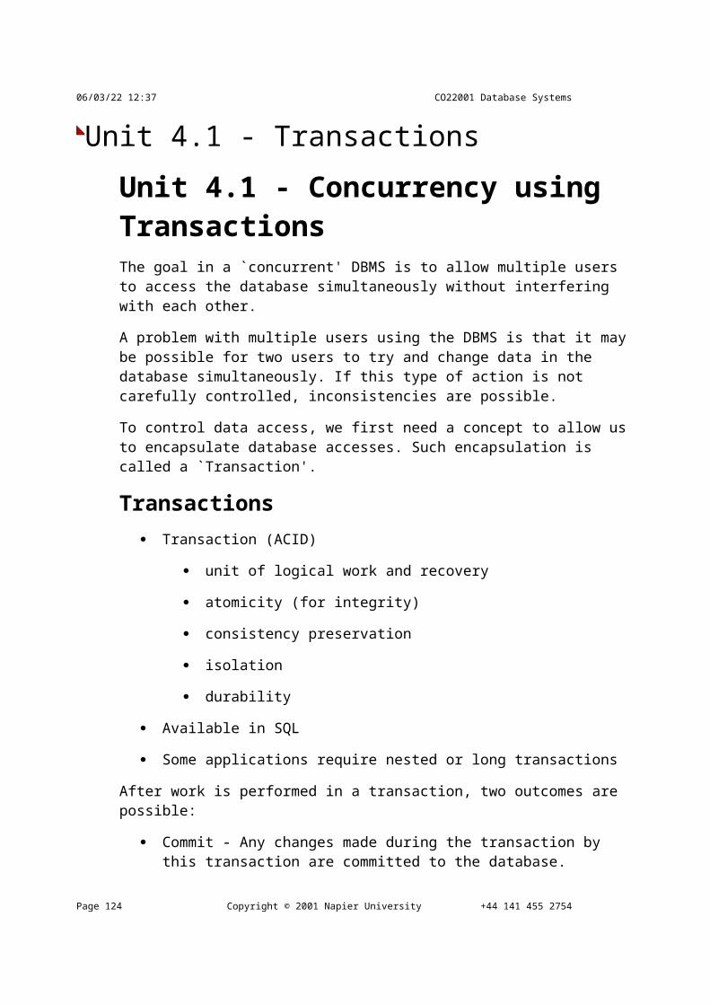
CO22001 Database Systems Student Notes
what effect this is going to have in the future. Future predictions can be made using the organisation's short and long-term plan.
Performance tuning - if the DBMS is slow for some tasks, then perhaps by manipulating the database the tasks can be speeded up.
DBA Tools To assist the DBA in his or her duties, a number of tools are available:
Loading routines
Reorganising routines
Journaling routines
Recovery routines
Statistical Analysis routines
Data Dictionary
DBMS Product Evaluation Another task performed by the DBA is the evaluation and comparison of DBMS's, so that the correct product can be selected to meet the database and customer specification. This cannot be done in isolation from the context in which the product will operate, and should be done before database implementation. Consider:
Price
Documentation
Support Agreements
Data Structurer supported
Performance
Tools
Data Structures Supported The DBA must select which data model to use. In this module on relation data models have really been considered. There are also object-oriented, hierarchical, and network models. Some data sets will fall naturally into one model. For instance, a hierarchical model can be specified as a network, but network has more overheads. The DBA must weigh up all the pros and cons of each model.
Note that the selection of DBMS should not occur until after proper business analysis, data analysis, and logical design. Thus model used should not be affected by the DBMS
Dr G. Russell Copyright © 2002 Napier University Page 125

08/05/23 15:04 CO22001 Database Systems
selected.
Performance Response depends on a variety of factors
Quality of software-implementation and engineering
Hardware support
CPU power
Main memory
Disks
Dedicated DB machine
Volume of data
Series of benchmarks available.
Tools Faculties offered in addition to DBMS, eg
Report writer
Forms generator
4GL
Query Language
Data Dictionary
How user-friendly are the tools?
Query language - adhere to any standard? (eg SQL for a relational DBMS)
If the DBMS selected is relational, one can check how it measures up against Codd's rules.
Page 126 Copyright © 2001 Napier University +44 141 455 2754

CO22001 Database Systems Student Notes
Unit 5.2b - SecurityUnit 5.2b - Security Security of the database involves the protection of the database against:
unauthorised disclosures
alteration
destruction
The protection which security gives is usually directed against two classes of user
Stop people without database access from having any form of access.
Stop people with database access from performing actions on the database which are not required to perform their duties.
There are many aspects to security
Legal, social and ethical aspects
Legally there is the Data Protection Act, which places restrictions on databases which contain information on living people. This was created to protect the public from data contained on a computer, about themselves, to which the public had previously no legal right of access. Information on computers can be wrong, and decisions made on wrong information concerns the public and additionally is of no benefit to the company holding the data. The act supports the idea of the public querying data, and indicating errors in that data.
However, just because a database is legal does not make it socially or ethically acceptable. Collating medical records on computer for a hospital is acceptable, but not having enough security to prevent insurance companies accessing the database and using that as a basis for rejecting life assurance applications could be considered questionable. Frequently is it best to place the tightest restrictions on who can access data, and where necessary security deliberately relaxed to allow only legitimate queries to take place.
Physical controls
Security often begins with physical controls. If a person cannot enter the building where the database runs and is accessed, then that person cannot access the database. Usually the construction of security is a layered approach, where a person bent on accessing the database must penetrate multiple levels of security. The simple precaution of having all the database access points behind locked doors can only add to the security of the system.
Policy questions
Dr G. Russell Copyright © 2002 Napier University Page 127

08/05/23 15:04 CO22001 Database Systems
Security of a database is often the enforcement in the database of the company policy. All companies should have a policy statement, listing what is acceptable and what is not. Companies with weak policy statements will often have the weakest security. At a minimum, it should be policy that data stored in the database should not be made available to outside agents without written consent from a Managing Director. Without a policy statement, it is hard to argue that an employee has actually done anything wrong...
Operational problems
If only a single person has access to a database, security is certainly higher than if many people have access. However, if all the people in the UK had to phone the same one person to find out what their bank balance was the whole system would quickly become unworkable. Security considerations often have to be balanced against operational issues.
Hardware controls
No matter how secure the database actually is, if a person can simply steal the hard drive on which the database is stored, then that person can access the database at leisure. This case is obvious, but less obvious security failures, such as taking a copy of a backup tape of the database, can be harder to safeguard against.
Operating system security
Most DBMS's run on top of an operating system (OS). Examples of OS's include Window 95, Windows NT, and Unix. The database may be secure from within the DBMS, but if the database can also be accessed from the OS using simple file handling programs, then a clear weakness in the security model exists.
Database system security
Within the DBMS itself, if anyone can access anything then having any other sort of security seems pointless. The use of user accounts and password protection of user identities is a good starting point to improve security. User identities is also an aid to accountability. Protection of certain elements of the database with respect to certain users (or user groups) should always be considered where potentially confidential data is being stored. It is DBMS security which is the focus of this discussion.
Granularity of DBMS Security The unit of data used in specifying security in the database can be, for example;
the entire database
a set of relations
individual relation
a set of tuples in a relation Page 128 Copyright © 2001 Napier University +44 141 455 2754

CO22001 Database Systems Student Notes
individual tuple
a set of attributes of all tuples
an attribute of an individual tuple.
DBMS-level Protection Data encryption:
Often it is hard to prevent people from copying the database and then hacking into the copy at another location. It is easier to simply make copying the data a useless activity by encrypting the data. This means that the data itself is unreadable unless you know a secret code. The encrypted data in combination with the secret key is needed to use the DBMS.
Audit Trails:
If someone does penetrate the DBMS, it is useful to find out how they did it and what was accessed or altered. Audit Trails can be set up selectively to minimise disk usage, identify system weaknesses, and finger naughty users.
User-level Security for SQL Each user has certain access rights on certain objects.
Different users may have different access rights on the same object.
In order to control the granularity of access rights, users can
Have rights of access (authorisations) on a table
Have rights of access on a view. Using views, access rights can be controlled horizontal and vertical subsets on a table, and on dynamically generated data from other tables.
Naming Hierarchy In a DBMS, there is a two layer approach to naming relations.
The DBMS is made up of a number of `databases'. The Database Administrator (DBA) has permission to create and delete databases, and to grant users access to databases.
Each database is a flat name space. Users with the necessary permission can create tables and views in a database. Because it is a flat name space, all table names must be unique within a database. The DBMS helps users in this regard:
table and view names are prepended with the name of the user who created it.
Dr G. Russell Copyright © 2002 Napier University Page 129
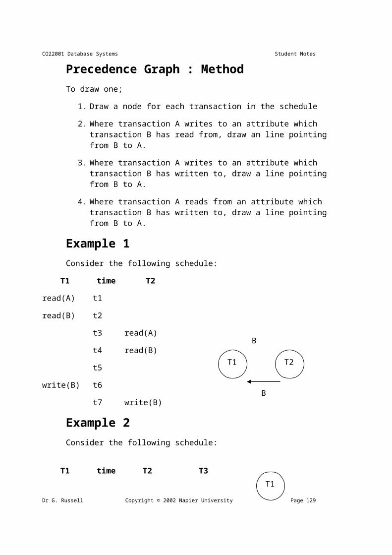
08/05/23 15:04 CO22001 Database Systems
the database login name is often taken as the username.
By way of an example, consider a table `hello' created by a user jbloggs.
The table will have the name jbloggs.hello
The user jbloggs can access the table using the name `hello'
Other users must use the table's full name to access the table
The user jbloggs can control who has access to the table using the GRANT command.
If the DBA creates a table, and makes it available to PUBLIC, then no user needs to specify the full table name in order to access it.
The GRANT command GRANT is used to grant privileges to users
GRANT privileges ON tablename TO { grantee ... } [ WITH GRANT OPTION ]
Possible privileges are:
SELECT - user can retrieve data
UPDATE - user can modify existing data
DELETE - user can remove data
INSERT - user can insert new data
REFERENCES - user can make references to the table
The WITH GRANT OPTION permits the specified user can grant privileges which that user possesses on that table to other users. This is a good way to permit other users to look after permissions for certain tables, such as allowing a manager to control access to a table for his or her subordinates.
grantee need not be a username or a set of usernames. It is permitted to specify PUBLIC, which means that the privileges are granted to everyone.
GRANT SELECT ON userlist TO PUBLIC;
Page 130 Copyright © 2001 Napier University +44 141 455 2754

CO22001 Database Systems Student Notes
Unit 5.3 - Data DictionaryUnit 5.3 - Data DictionaryA Data Dictionary System (DDS) is a software tool for recording and processing data about the data (metadata) that an organisation uses and processes. Originally DDS were designed as documentation tools, ensuring standard terminology for data items (and sometimes programs) and providing a cross reference capability. They have now evolved as an essential feature of the systems environment and as a tool for the DBA to keep track of data on the database and control its use. This helps to minimise maintenance and development costs.
A DDS is a central catalogue of the definitions and usage of the data within an organization. It can be used as a stand alone tool or integrated with a DBMS. Most DDS are used chiefly as a documentation aid and as a control point for referencing data. They may also play an active role in systems design, programming and in running systems. It could be used to provide the data structures to the program at compile time or validate data at execution time. It can be used as a storage base of programming code (sub-programs) and these subprograms may be used in a number of programs.
Benefits of a DDS Benefits of a DDS are mainly due to the fact that it is a central store of information about the database.
Benefits include
improved documentation and control
consistency in data use
easier data analysis
reduced data redundancy
simpler programming
the enforcement of standards
better means of estimating the effect of change.
DDS Facilities A DDS should provide two sets of facilities:
To record and analyse data requirements independently of how they are going to be met conceptual data models.
To record and design decisions in terms of database or file structures Dr G. Russell Copyright © 2002 Napier University Page 131

08/05/23 15:04 CO22001 Database Systems
implemented and the programs which access them internal schema.
The conceptual view shows a model of the organisation, that is, the entities, their attributes, and the relationship between these entities. This model is a result of the data analysis process and is therefore independent of any data processing implications. The conceptual view can also include details of the events and operations that occur in the organisation. It represents the conceptual schema.
The implementation view gives information about the data processing applications in computing terms. The processes are therefore described as systems, programs and sub-programs. The data is described in terms of files, records and fields.
One of the main functions of a DDS is to show the relationship between the conceptual and implementation views. The mapping should be consistent - inconsistencies are an error and can be detected here.
DD Information The names associated with that element (aliases)
A description of the data element in natural language.
Details of ownership.
Details of users that refer to the element.
Details of the systems and programs which refer to or update the element.
Details on any privacy constraints that should be associated with the item.
Details about the data element in data processing systems, such as the length of the data item in characters, whether it is numeric alphabetic or another data type, and what logical files include the data item.
The security level attached to the element in order to control access.
The total storage requirement.
The validation rules for each element (e.g. acceptable values).
Details of the relationship of the data items to others.
DD Management With so much detail held on the DDS, it is essential that an indexing and cross-
referencing facility is provided by the DDS.
The DDS can produce reports for use by the data administration staff (to investigate the efficiency of use and storage of data), systems analysts, programmers, and users.
DDS can provide a pre-printed form to aid data input into the database and DD. Page 132 Copyright © 2001 Napier University +44 141 455 2754

CO22001 Database Systems Student Notes
A query language is provided for ad-hoc queries. If the DD is tied to the DBMS, then the query language will be that of the DBMS itself.
Management Objectives From an management point of view, the DDS should
provide facilities for documenting information collected during all stages of a computer project.
provide details of applications usage and their data usage once a system has been implemented, so that analysis and redesign may be facilitated as the environment changes.
make access to the DD information easier than a paper-based approach by providing crossreferencing and indexing facilities.
make extension of the DD information easier.
encourage systems analysts to follow structured methodologies.
Advanced Facilities Extra facilities which may be supported by DDS are:
Automatic input from source code of data definitions (at compile time).
The recognition that several versions of the same programs or data structures may exist at the same time.
live and test states of the programs or data.
programs and data structures which may be used at different sites.
data set up under different software or validation routine.
The provision of an interface with a DBMS.
Security features such as password protection, to restrict DDS access.
Generation of update application programs and programs to produce reports and validation routines.
Management AdvantagesA number of possible benefits may come from using a DDS:
A DDS can improve the ability of management to control and know about the data resource of the enterprise.
It can also show all the program files and reports that may be affected by any change to the definition or usage of data elements and possibly to generate code
Dr G. Russell Copyright © 2002 Napier University Page 133
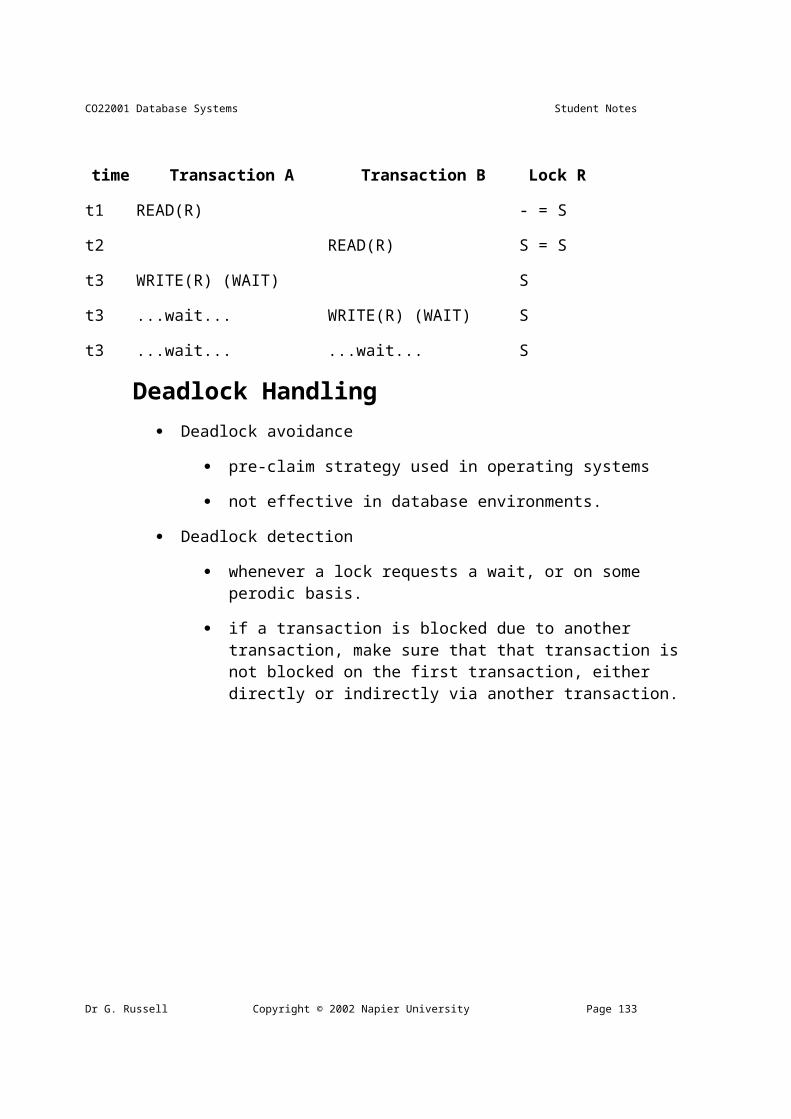
08/05/23 15:04 CO22001 Database Systems
which reflects that change. This allows accurate assessment of cost and time scale to effect any change.
A DDS reduces the clerical load of database administration. It gives the DBA more control over the design and use of the data base.
Accurate data definitions can be provided directly to program. Sensitive data can be made available only to particular users. Files and programs can be checked to ensure that standards are being followed.
A DDS can aid the recording, processing, storage and destruction of data and associated documents flowing through an organisation.
A DDS can help systems development by generating test files and providing documentation.
A DDS provides application programs with data definitions and subroutines and therefore enforces some standards on programming, making programs more readable and consistent.
A DDS aids application program maintenance because changes to the data and the data structures can be made where appropriate to all programs using the data.
A DDS aids the operations side of computing by holding details of storage and recovery procedures, and archiving information.
A DDS can provide effective security features such as passwords to assist in the protection of the data resource.
Management Disadvantages A DDS is a useful management tool, but at a price.
The DDS 'project' may itself take two or three years.
It needs careful planning, defining the exact requirements designing its contents, testing, implementation and evaluation.
The cost of a DDS includes not only the initial price of its installation and any hardware requirements, but also the cost of collecting the information entering it into the DDS, keeping it uptodate and enforcing standards.
The use of a DDS requires management commitment, which is not easy to achieve, particularly where the benefits are intangible and long term.
Page 134 Copyright © 2001 Napier University +44 141 455 2754
CO22001 Database Systems Student Notes
Tutorial - ER Modelling 1Tutorial - ER Diagram Examples 1-2Example 1 A publishing company produces scientific books on various subjects. The books are written by authors who specialize in one particular subject. The company employs editors who, not necessarily being specialists in a particular area, each take sole responsibility for editing one or more publications. A publication covers essentially one of the specialist subjects and is normally written by a single author. When writing a particular book, each author works with on editor, but may submit another work for publication to be supervised by other editors. To improve their competitiveness, the company tries to employ a variety of authors, more than one author being a specialist in a particular subject.
Example 2A General Hospital consists of a number of specialized wards (such as Maternity, Paediatry, Oncology, etc). Each ward hosts a number of patients, who were admitted on the recommendation of their own GP and confirmed by a consultant employed by the Hospital. On admission, the personal details of every patient are recorded. A separate register is to be held to store the information of the tests undertaken and the results of a prescribed treatment. A number of tests may be conducted for each patient. Each patient is assigned to one leading consultant but may be examined by another doctor, if required. Doctors are specialists in some branch of medicine and may be leading consultants for a number of patients, not necessarily from the same ward.
Tutorial - ER Modelling 2Tutorial - ER Diagram Examples 3-5Example 3A database is to be designed for a Car Rental Co. (CRC). The information required includes a description of cars, subcontractors (i.e. garages), company expenditures, company revenues and customers. Cars are to be described by such data as: make, model, year of production, engine size, fuel type, number of passengers, registration number, purchase price, purchase date, rent price and insurance details. It is the company policy not to keep any car for a period exceeding one year. All major repairs and maintenance are done by subcontractors (i.e. franchised garages), with whom CRC has long-term agreements. Therefore the data about garages to be kept in the database includes garage names, addressees, range of services and the like. Some garages require payments immediately after a repair has been made; with others CRC has made arrangements for
Dr G. Russell Copyright © 2002 Napier University Page 135
08/05/23 15:04 CO22001 Database Systems
credit facilities. Company expenditures are to be registered for all outgoings connected with purchases, repairs, maintenance, insurance etc. Similarly the cash inflow coming from all sources - car hire, car sales, insurance claims - must be kept of file.CRC maintains a reasonably stable client base. For this privileged category of customers special credit card facilities are provided. These customers may also book in advance a particular car. These reservations can be made for any period of time up to one month. Casual customers must pay a deposit for an estimated time of rental, unless they wish to pay by credit card. All major credit cards care accepted. Personal details (such as name, address, telephone number, driving licence, number) about each customer are kept in the database.
Example 4A database is to be designed for a college to monitor students' progress throughout their course of study. The students are reading for a degree (such as BA, BA(Hons) MSc, etc) within the framework of the modular system. The college provides a number of module, each being characterised by its code , title, credit value, module leader, teaching staff and the department they come from. A module is co-ordinated by a module leader who shares teaching duties with one or more lecturers. A lecturer may teach (and be a module leader for) more than one module. Students are free to choose any module they wish but the following rules must be observed: some modules require pre-requisites modules and some degree programmes have compulsory modules. The database is also to contain some information about students including their numbers, names, addresses, degrees they read for, and their past performance (i.e. modules taken and examination results).
Example 5 A relational database is to be designed for a medium sized Company dealing with industrial applications of computers. The Company delivers various products to its customers ranging from a single application program through to complete installation of hardware with customized software. The Company employs various experts, consultants and supporting staff. All personnel are employed on long-term basis, i.e. there are no short-term or temporary staff. Although the Company is somehow structured for administrative purposes (that is, it is divided into departments headed by department managers) all projects are carried out in an inter-disciplinary way. For each project a project team is selected, grouping employees from different departments, and a Project Manager (also an employee of the Company) is appointed who is entirely and exclusively responsible for the control of the project, quite independently of the Company's hierarchy. The following is a brief statement of some facts and policies adopted by the Company.
Page 136 Copyright © 2001 Napier University +44 141 455 2754
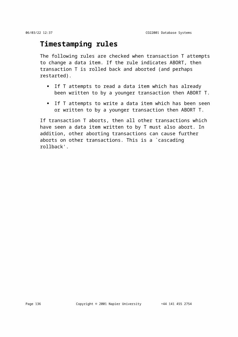
CO22001 Database Systems Student Notes
Multiple Choice TutorialMultiple Choice - HOWTO The first diet exam for databases is often a Multiple Choice exam paper. The second diet (the resit paper) is more usually a written paper. However, be prepared for either multiple choice or a written paper. It should not affect your study method, and if it does you are doing something wrong.
Here are a couple of useful guides to a successful multiple-choice exam.
1. Look at each question in turn.
2. Score out answers on the question sheet which are obviously wrong.
3. Do not be afraid of going onto the next question if no single correct answer can be selected immediately.
4. Read each question CAREFULLY. Are you selecting a TRUE answer or a FALSE answer from the options?
5. Try not to revisit answers before attempting all the other questions.
The Answer Sheet There are a few different answer sheets in use for this exam. It is ALWAYS best to read the instructions given with the exam, and any comments which the invigilator gives you. In some cases the exam may be automatically scanned and marked by computer, which may require you to use a very specific way of entering the answers.
The answer sheet shown here is the one first used in this module, and is still used where electronic support for automatic marking is not available. In all exams there may be a box for your full name. Napier currently uses an anonymous marking system, so do not enter your name unless you are uncertain if you have entered your Matrix No correctly. Every year there are still a few students who seem unable to write in their Matrix No properly and legibly.
Dr G. Russell Copyright © 2002 Napier University Page 137

08/05/23 15:04 CO22001 Database Systems
Matrix No:
Full Name: ______________________________
QABCDE Q ABCDE
1 6
2 7
3 8
4 9
5 10
Entering an answer
Entering A for Q1. Changing A to C in Q1.
QABCDE QABCDE
1 1
Changing C back to A in Q1.
QABCD E
1 A
Page 138 Copyright © 2001 Napier University +44 141 455 2754
CO22001 Database Systems Student Notes
Reason/Assertion
In past exams a number of REASON/ASSERTION question were used. For example
Assertion : Fire is hot to the touchReason : Fire needs Oxygen to burn
Option Assertion Reason Assertion BECAUSE reason
A True True REASON IS a valid reason...
B True True REASON IS NOT a valid reason...
C True False
D False True
E False False
The Assertion is TRUE, and the Reason is TRUE, but the Assertion is not true because of the Reason, so the answer is B.
Reason/Assertion questions are NO LONGER USED in current exams.
Dr G. Russell Copyright © 2002 Napier University Page 139

08/05/23 15:04 CO22001 Database Systems
Example
Now give the written Multiple Choice tutorial a try. Give yourself 30 minutes for the test. It is not assessed, and it does not count towards your final mark.
In a subsequent session, I will go over the assessment with you. Good luck!
1. A publishing company produces academic books on various subjects. Books are written by authors who specialise in one or more particular subject. The company employs a number of editors who do not have particular specialisations but who take sole responsibilty for for editing one or more publications. A publication covers a single subject area but may be written by one or more author - the contribution of each author is recorded as a percentage for the purposes of calculating royalties.
The following ER diagram is intended to represent the above specification:
author subject
contribution
publication editor
specialises in
makes
to
is about
edits
Indicate the relation which has an incorrect cardinality shown:
A. specialises in
B. makes
C. is about
D. to
E. None of the above
2. The specification is to be changed so that an author can develop a publication covering more than one subject area and that the schema must be able to store the
Page 140 Copyright © 2001 Napier University +44 141 455 2754

CO22001 Database Systems Student Notes
percentage of the compents concerned with each of the subjects. Select an appropriate change to the ER diagram:
A. publication-subject becomes many to many
B. author-subject becomes many to many
C. author-publication becomes many to many
D. more than one of the above
E. none of the above
3. Consider the relational schema R(A,B,C,D,E) with non-key functional dependencies C,D - E and B - C.
Select the strongest statement that can be made about the schema R
A. R is in first normal form
B. R is in second normal form
C. R is in third normal form
D. R is in BCNF normal form
E. None of the above
4. Locking was introduced into databases so that
A. Keys can be provided to maintain security.
B. Reading and writing is possible.
C. All simultaneous transactions are prevented.
D. Passwords can be provided to maintain security
E. Consistency can be enforced.
5. When accessing a disk block, the seek time
A. is insignificant in comparison to transfer times
B. is about the same as transfer times
C. greatly exceeds transfer times
Dr G. Russell Copyright © 2002 Napier University Page 141

08/05/23 15:04 CO22001 Database Systems
D. is the time taken to search for data in a sorted list of database rows
E. is measured in nanoseconds
6. Hash-table insertions
A. avoid hash-collisions by manipulating the foreign keys
B. might use hash-chains to allow hash-collisions
C. use balanced binary trees to allow hash-collisions
D. use primary keys to avoid hash-collisions
E. become unusable if there are any hash-collisions
7. When a transaction aborts
A. all users must be notified
B. all changes it has made are immediately available to other transactions
C. the modifications of all transactions currently running are also aborted
D. it can abort transactions which have already committed
E. it releases all of its locks
8. Films Database
Consider the following database:MOVIE(id,title,yr)ACTOR(id,name)CASTING(movieid,actorid)
Assertion Reason
The films database is NOT in BCNF The table CASTING has a composite key
Option Assertion Reason Assertion BECAUSE reason
A True True REASON IS a valid reason...
B True True REASON IS NOT a valid reason...
C True False
Page 142 Copyright © 2001 Napier University +44 141 455 2754

CO22001 Database Systems Student Notes
D False True
E False False
9. Using the same Films Database, identify the SQL command which will return the titles of all 1959 Marilyn Monroe films.
A. The following SQL...
SELECT title FROM movie,casting,actor WHERE movieid = movie.id AND name = 'Marilyn Monroe' ;
B. The following SQL...
SELECT title FROM movie,actor WHERE name = 'Marilyn Monroe' AND yr = 1959 ;
C. The following SQL...
SELECT title FROM movie,casting,actor WHERE movieid = movie.id AND actor.id = actorid AND name = 'Marilyn Monroe' AND yr = 1959 ;
D. The following SQL...
SELECT title FROM movie,casting,actor WHERE movieid = movie.id AND actor.id = actorid AND movie.yr = casting.yr AND name = 'Marilyn Monroe' AND yr = 1959 ;
E. None of the above
10. Consider the relational schema R(A,B,C,D,E) with non-key functional dependencies C,D - E and B - C.
Assertion Reason
In the relation R (above) the functional dependency C,D-E is transitive C and D do NOT contribute to the
primary key
Dr G. Russell Copyright © 2002 Napier University Page 143
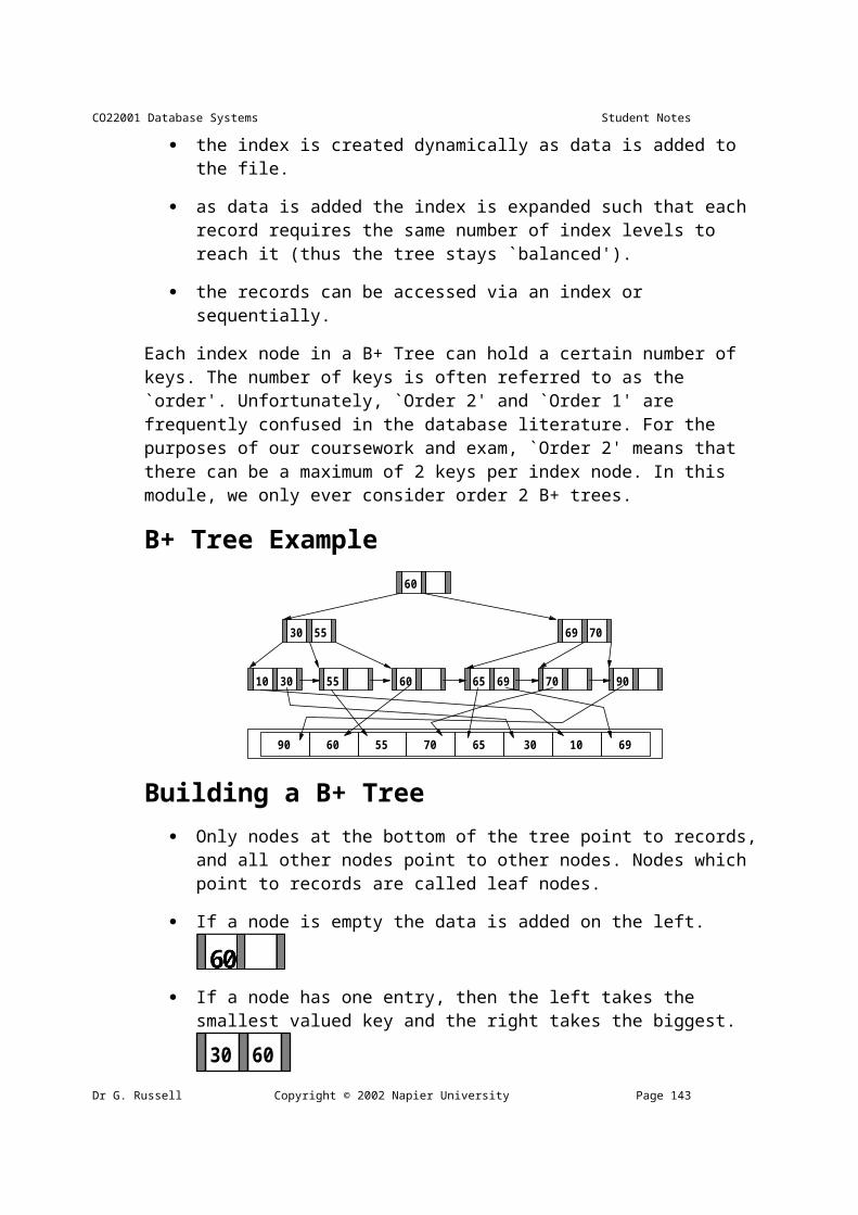
08/05/23 15:04 CO22001 Database Systems
Option Assertion Reason Assertion BECAUSE reason
A True True REASON IS a valid reason...
B True True REASON IS NOT a valid reason...
C True False
D False True
E False False
Page 144 Copyright © 2001 Napier University +44 141 455 2754