Datasets of the Unsupervised and Transfer Learning Challenge · Datasets of the Unsupervised and...

Datasets of the Unsupervised and Transfer Learning Challenge

Report prepared by Isabelle Guyon with information from the data donors listed below: Handwriting recognition (AVICENNA) -- Reza Farrahi Moghaddam, Mathias Adankon, Kostyantyn Filonenko, Robert Wisnovsky, and Mohamed Chériet (Ecole de technologie supérieure de Montréal, Quebec) contributed the dataset of Arabic manuscripts. Human action recognition (HARRY) -- Ivan Laptev and Barbara Caputo collected and made publicly available the KTH human action recognition datasets. Marcin Marszalek, Ivan Laptev and Cordelia Schmid collected and made publicly available the Hollywood 2 dataset of human actions and scenes. Object recognition (RITA) -- Antonio Torralba, Rob Fergus, and William T. Freeman, collected and made available publicly the 80 million tiny image dataset. Vinod Nair and Geoffrey Hinton collected and made available publicly the CIFAR datasets . See the techreport Learning Multiple Layers of Features from Tiny Images, by Alex Krizhevsky, 2009, for details.Ecology (SYLVESTER) -- Jock A. Blackard, Denis J. Dean, and Charles W. Anderson of the US Forest Service, USA, collected and made available the (Forest cover type ) dataset. Text processing (TERRY) -- David Lewis formatted and made publicly available the RCV1-v2 Text Categorization Test Collection derived from REUTER news clips.The toy example (ULE) is the MNIST handwritten digit database made available by Yann LeCun and Corinna Costes.

Table 1: Datasets of the unsupervised and transfer learning challenge.

Dataset Domain Feat. num.

Sparsity (%)

Development num.

Transfer num.

Validation num.

Final Eval. num.

Data (text)

Data (Matlab)

AVICENNA Arabic

manuscripts 120 0.00 150205 50000 4096 4096

16

MB 14 MB

HARRY

Human

action

recognition

5000 98.12 69652 20000 4096 4096 13

MB 15 MB

RITA Object

recognition 7200 1.19 111808 24000 4096 4096

1026

MB 762 MB

SYLVESTER Ecology 100 0.00 572820 100000 4096 4096 81

MB 69 MB

TERRY Text

recognition 47236 99.84 217034 40000 4096 4096

73

MB 56 MB

ULE (toy

data)

Handwritten

digits 784 80.85 26808 10000 4096 4096 7 MB 13 MB

Data formats: All the data sets are in the same format; xxx should be replaced by one of: devel: development data valid: evaluation data used as validation set final: final evaluation data The participant have access only to the files outlined in red: dataname.param: Parameters and statistics about the data dataname_xxx.data: Unlabeled data (a matrix of space delimited numbers, patterns in lines, features in columns). dataname_xxx.mat: The same data matrix in Matlab format in a matrix called X_xxx. dataname_transfer.label: Target values provided for transfer learning only. Multiple labels (1 per column), label values are -1, 0, or 1 (for negative class, unknown, positive class). dataname_valid.label: Target values, not provided to participants. dataname_final.label: Target values, not provided to participants. dataname_xxx.dataid: Identity of the samples (lines of the data matrix). dataname_xxx.labelid: Identity of the labels (variables that are target values, i.e., columns of the label matrix.) dataname.classid: strings representing the names of the classes. The participants will use the following formats results: dataname_valid.prepro: Preprocessed data send during the development phase. dataname_final.prepro : Preprocessed data for the final submission. Metrics The data representations are assessed automatically by the evaluation platform connected to this website. To each evaluation set (validation set or final evaluation set) the organizers have assigned several binary classification tasks unknown to the participants. The platform will use the data representations provided by the participants to train a linear classifier (code provided in Appendix A) to solve these tasks. To that end, the evaluation data (validation set or final evaluation set) are partitioned randomly into a training set and a test set. The parameters of the linear classifier are adjusted using the training set. Then, predictions are made on test data using the trained model. The Area Under the ROC curve (AUC) is computed to assess the performance of the linear classifier. The results are averaged over all tasks and over several random splits into a training set and a complementary test set. The number of training examples is varied and the AUC is plotted against the number of training examples in a log scale (to emphasize the results on small numbers of training examples). The area under the learning curve (ALC) is used as scoring metric to synthesize the results. The participants are ranked by ALC for each individual dataset. The participants having submitted a complete experiment (results on all 5 datasets of the challenge) enter the final ranking. The winner is determined by the best average rank over all datasets for the results of their last complete experiment.

Global Score: The Area under the Learning Curve (ALC) The prediction performance is evaluated according to the Area under the Learning Curve (ALC). A learning curve plots the Area Under the ROC curve (AUC) averaged over all the binary classification tasks and all evaluation data splits. The AUC is the area of the curve that plots the sensitivity (error rate of the “positive class”) vs. the specificity (error rate of the “negative class).

We consider two baseline learning curves:

1. The ideal learning curve, obtained when perfect predictions are made (AUC=1). It goes up vertically then follows AUC=1 horizontally. It has the maximum area "Amax".

2. The "lazy" learning curve, obtained by making random predictions (expected value of AUC: 0.5). It follows a straight horizontal line. We call its area "Arand".

To obtain our ranking score displayed in Mylab and on the Leaderboard, we normalize the ALC as follows: global_score = (ALC-Arand)/(Amax-Arand) For simplicity, we call ALC the normalized ALC or global score. We show in Figure A3 examples of learning curves for the toy example ULE, obtained using the sample code . Note that we interpolate linearly between points. The global score depends on how we scale the x-axis. We use a log2 scaling for all datasets.

A -- ULE This dataset is not part of the challenge. It is given as an example, for illustration purpose, together with ALL the labels.

1) Topic The task of ULE is handwritten digit recognition.

2) Sources a. Original owners

The data set was constructed from the MNIST data that is made available by Yann LeCun of the NEC Research Institute at http://yann.lecun.com/exdb/mnist/. The digits have been size-normalized and centered in a fixed-size image of dimension 28x28. We show examples of digits in Figure B1.

50 100 150 200 250

20

40

60

80

100

120

140

Figure A1: Examples of digits from the MNIST database.

Table A1: Number of examples in the original data Digit 0 1 2 3 4 5 6 7 8 9Total Training 5923 6742 5958 6131 5842 5421 5918 6265 5851 5949 60000Test 980 1135 1032 1010 982 892 958 1028 974 1009 10000Total 6903 7877 6990 7141 6824 6313 6876 7293 6825 6958 70000

b. Donor of database

This version of the database was prepared for the “unsupervised and transfer learning challenge” by Isabelle Guyon, 955 Creston Road, Berkeley, CA 94708, USA ([email protected]).

c. Date prepared for the challenge: November 2010.

3) Past usage

Many methods have been tried on the MNIST database, in its original data split (60,000 training examples, 10,000 test examples, 10 classes.) Here is an abbreviated list from http://yann.lecun.com/exdb/mnist/: Table A2: Previous results for MNIST (ULE)

METHOD TEST ERROR RATE (%)

linear classifier (1-layer NN) 12.0

linear classifier (1-layer NN) [deskewing] 8.4

pairwise linear classifier 7.6

K-nearest -neighbors, Euclidean 5.0

K-nearest -neighbors, Euclidean, deskewed 2.4

40 PCA + quadratic classifier 3.3

1000 RBF + linear classifier 3.6

K-NN, Tangent Distance, 16x16 1.1

SVM deg 4 polynomial 1.1

Reduced Set SVM deg 5 polynomial 1.0

Virtual SVM deg 9 poly [distortions] 0.8

2-layer NN, 300 hidden units 4.7

2-layer NN, 300 HU, [distortions] 3.6

2-layer NN, 300 HU, [deskewing] 1.6

2-layer NN, 1000 hidden units 4.5

2-layer NN, 1000 HU, [distortions] 3.8

3-layer NN, 300+100 hidden units 3.05

3-layer NN, 300+100 HU [distortions] 2.5

3-layer NN, 500+150 hidden units 2.95

3-layer NN, 500+150 HU [distortions] 2.45

LeNet-1 [with 16x16 input] 1.7

LeNet-4 1.1

LeNet-4 with K-NN instead of last layer 1.1

LeNet-4 with local learning instead of ll 1.1

LeNet-5, [no distortions] 0.95

LeNet-5, [huge distortions] 0.85

LeNet-5, [distortions] 0.8

Boosted LeNet -4, [distortions] 0.7

K-NN, shape context matching 0.67

This dataset was used in the NIPS 2003 Feature Selection Challenge under the name GISETTE and in the WCCI 2006 Performance Prediction Challenge and the IJCNN 2007 Agnostic Learning vs. Prior Knowledge Challenge under the name GINA.

References: Gradient-based learning applied to document recognition. Y. LeCun, L. Bottou, Y. Bengio, and P. Haffner. Proceedings of the IEEE, 86(11):2278-2324, November 1998. Result Analysis of the NIPS 2003 Feature Selection Challenge, Isabelle Guyon , Asa Ben Hur , Steve Gunn , Gideon Dror, Advances in Neural Information Processing Systems 17, MIT Press, 2004. Agnostic Learning vs. Prior Knowledge Challenge, Isabelle Guyon, Amir Saffari, Gideon Dror, and Gavin Cawley, In proceedings IJCNN 2007, Orlando, Florida, August 2007. Analysis of the IJCNN 2007 Agnostic Learning vs. Prior Knowledge Challenge, Isabelle Guyon, Amir Saffari, Gideon Dror, and Gavin Cawley, Neural Network special anniversary issue, in press. [Earlier draft] Hand on Pattern Recognition, challenges in data representation, model selection, and performance prediction. Book in preparation. Isabelle Guyon, Gavin Cawley, Gideon Dror, and Amir Saffari Editors.

4) Experimental design

We used the raw data: - The feature names are the (i,j) matrix coordinates of the pixels (in a 28x28

matrix.) - The data have gray level values between 0 and 255. - The validation set and the final test set have approximately even numbers of

examples for each class.

5) Number of examples and class distribution

Table A3: Data statistics for ULE


Sparsity (%)

Development num.

Transfer num.

Validation num

Final eval. num.

ULE Handwriting 784 80.85 26808 10000 4096 4096

All variables are numeric (no categorical variable). There are no missing values. The target variables are categorical. Here is class label composition of the data subsets:

Validation set: X[4096, 784] Y[4096, 1] One: 1370 Three: 1372 Seven: 1354 Final set: X[4096, 784] Y[4096, 1] Zero: 1376 Two: 1373 Six: 1347 Development set: X[26808, 784] Y[26808, 1] Zero: 2047 One: 2556 Two: 2089 Three: 2198 Four: 3426 Five: 3179 Six: 2081 Seven: 2314 Eight: 3470 Nine: 3448 Transfer labels (10000 labels): Four: 2562 Five: 2301 Eight: 2564 Nine: 2573

6) Type of input variables and variable statistics

The variables in raw data are pixels. We also produced baseline results using as variables Gaussian RBF values with 20 cluster centers generated by the Kmeans clustering algorithm. The algorithm was run on the validation set and the final evaluation set separately. The development set and the transfer labels were not used. The cluster centers are shown in Figure A2.

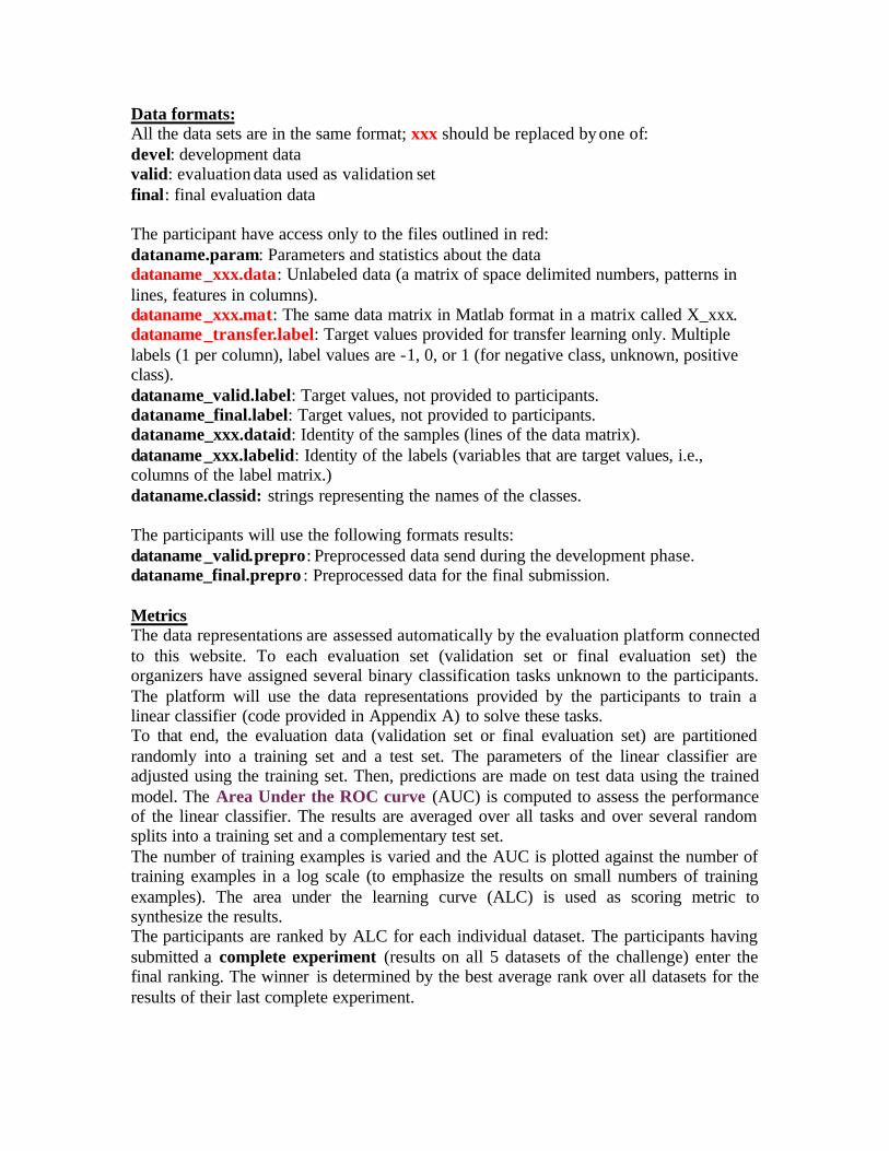
7) Baseline results We used a linear classifier making independence assumptions between variables, similar to Naïve Bayes, to generate baseline learning curves from raw data and preprocessed data. The normalized ALC (score used in the challenge) are shown in Figures A3 and A4 and summarized in Table A4.

Table A4: Baseline results (normalized ALC for 64 training examples). ULE Valid Final Raw 0.7905 0.7169 Preprocessed 0.8416 0.3873

Validation set cluster centers

Final evaluation set cluster centers

Figure A2: Clusters obtained by Kmeans clustering

Figure A3: Baseline results on raw ULE data. Top: valid. set.Bottom: final eval. set.

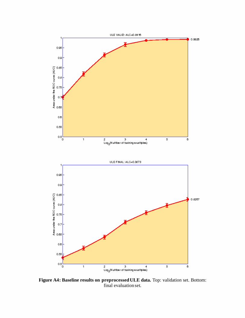
Figure A4: Baseline results on preprocessed ULE data. Top: validation set. Bottom:

final evaluation set.

B - AVICENNA

1) Topic

The AVICENNA dataset provides a feature representation of Arabic Historical Manuscripts.

2) Sources a. Original owners The dataset is prepared on manuscript images provided by The Institute of Islamic Studies (IIS), McGill. Manuscript author: Abu al-Hasan Ali ibn Abi Ali ibn Muhammad al-Amidi (d. 1243 or 1233) Manuscript title: Kitab Kashf al-tamwihat fi sharh al-Tanbihat (Commentary on Ibn Sina's al-Isharat wa-al-tanbihat) Brief description: Among the works of Avicenna, his al-Isharat wa-al-tanbihat received the attention of the later scholars more than others. The reception of this work is particularly intensive and widespread in the period between the late twelfth century to the first half of the fourteenth century, when more than a dozen comprehensive commentaries on this work were composed. These commentaries were one of the main ways of approaching, understanding and developing Avicenna’s philosophy and therefore any study of Post-Avicennian philosophy needs to pay specific attention to this commentary tradition. Kashf al-tamwihat fi sharh al-Tanbihat by Abu al-Hasan Ali ibn Abi Ali ibn Muhammad al-Amidi (d. 1243 or 1233), one of the early commentaries written on al-Isharat wa-al-tanbihat, is an unpublished commentary which still await scholars' attention.

a. Donors of the database

Reza Farrahi Moghaddam, Mathias Adankon, Kostyantyn Filonenko, Robert Wisnovsky, and Mohamed Cheriet. Contact: Mohamed Cheriet Synchromedia Laboratory ETS, Montréal, (QC) Canada H3C 1K3 [email protected] Tel: +1(514)396-8972 Fax: +1(514)396-8595

b. Date received: December 2010

3) Past usage : Part of the data was used in the active learning challenge (http://clopinet.com/al).

4) Experimental design The features were extracted following the procedure described in the JMLR W&CP paper: IBN SINA: A database for handwritten Arabic manuscripts understanding research, by Reza Farrahi Moghaddam, Mathias Adankon, Kostyantyn Filonenko, Robert Wisnovsky, and Mohamed Chériet. The original data includes 92 numeric features. We added 28 distracters then rotated the feature space with a random rotation matrix. Finally, the features were quantized and rescaled between 0 and 999.

5) Data statistics Table B1: Data statistics for AVICENNA.


Sparsity (%)

Development num.

Transfer num.

Validation num.

Final Eval. num.

AVICENNA Arabic manuscripts 120 0 150205 50000 4096 4096

Table B2: Original feature statistics

Name Type Min Max Num val Aspect_ratio continuous 0 999 395 Horizontal_frequency ordinal 1 13 13 Vertical_CM_ratio continuous 0 999 539 Singular_points continuous 0 238 51 Height_ratio continuous 0 999 163 Hole_feature binary 0 1 2 End_points continuous 0 72 43 Dot_feature binary 0 1 2 BP_hole_1 binary 0 1 2 BP_EP_1 binary 0 1 2 BP_BP_1 binary 0 1 2 BP_hole_2 binary 0 1 2 BP_EP_2 binary 0 1 2 BP_BP_2 binary 0 1 2 BP_hole_3 binary 0 1 2 BP_EP_3 binary 0 1 2 BP_BP_3 binary 0 1 2 BP_hole_4 binary 0 1 2 BP_EP_4 binary 0 1 2 BP_BP_4 binary 0 1 2 BP_hole_5 binary 0 1 2 BP_EP_5 binary 0 1 2 BP_BP_5 binary 0 1 2 BP_hole_6 binary 0 1 2 BP_EP_6 binary 0 1 2 BP_BP_6 binary 0 1 2

EP_BP_1 binary 0 1 2 EP_EP_1 binary 0 1 2 EP_VCM_1 ordinal 0 2 3 EP_BP_2 binary 0 1 2 EP_EP_2 binary 0 1 2 EP_VCM_2 ordinal 0 2 3 EP_BP_3 binary 0 1 2 EP_EP_3 binary 0 1 2 EP_VCM_3 ordinal 0 2 3 EP_BP_4 binary 0 1 2 EP_EP_4 binary 0 1 2 EP_VCM_4 ordinal 0 2 3 EP_BP_5 binary 0 1 2 EP_EP_5 binary 0 1 2 EP_VCM_5 ordinal 0 2 3 EP_BP_6 binary 0 1 2 EP_EP_6 binary 0 1 2 EP_VCM_6 ordinal 0 2 3 BP_dot_UP_1 binary 0 1 2 BP_dot_DOWN_1 binary 0 1 2 BP_dot_UP_2 binary 0 1 2 BP_dot_DOWN_2 binary 0 1 2 BP_dot_UP_3 binary 0 1 2 BP_dot_DOWN_3 binary 0 1 2 BP_dot_UP_4 binary 0 1 2 BP_dot_DOWN_4 binary 0 1 2 BP_dot_UP_5 binary 0 1 2 BP_dot_DOWN_5 binary 0 1 2 BP_dot_UP_6 binary 0 1 2 BP_dot_DOWN_6 binary 0 1 2 EP_dot_1 binary 0 1 2 EP_dot_2 binary 0 1 2 EP_dot_3 binary 0 1 2 EP_dot_4 binary 0 1 2 EP_dot_5 binary 0 1 2 EP_dot_6 binary 0 1 2 Dot_dot_1 binary 0 1 2 Dot_dot_2 binary 0 1 2 Dot_dot_3 binary 0 1 2 Dot_dot_4 binary 0 1 2 Dot_dot_5 binary 0 1 2

Dot_dot_6 binary 0 1 2 EP_S_Shape_1 ordinal 0 2 3 EP_clock_1 ordinal 0 3 4 EP_UP_BP_1 binary 0 1 2 EP_DOWN_BP_1 binary 0 1 2 EP_S_Shape_2 ordinal 0 2 3 EP_clock_2 ordinal 0 3 4 EP_UP_BP_2 binary 0 1 2 EP_DOWN_BP_2 binary 0 1 2 EP_S_Shape_3 ordinal 0 2 3 EP_clock_3 ordinal 0 3 4 EP_UP_BP_3 binary 0 1 2 EP_DOWN_BP_3 binary 0 1 2 EP_S_Shape_4 ordinal 0 2 3 EP_clock_4 ordinal 0 3 4 EP_UP_BP_4 binary 0 1 2 EP_DOWN_BP_4 binary 0 1 2 EP_S_Shape_5 ordinal 0 2 3 EP_clock_5 ordinal 0 3 4 EP_UP_BP_5 binary 0 1 2 EP_DOWN_BP_5 binary 0 1 2 EP_S_Shape_6 ordinal 0 2 3 EP_clock_6 ordinal 0 3 4 EP_UP_BP_6 binary 0 1 2 EP_DOWN_BP_6 binary 0 1 2

There are no missing values. The data were split as follows:

Validation set: X[4096, 120] Y[4096, 5] EU: 1113 HU: 875 bL: 1105 jL: 837 tL: 1110 Final set: X[4096, 120] Y[4096, 5] dL: 966 hL: 1188 kL: 896 qL: 982 sL: 863 Development set: X[150205, 120] Y[150205, 52] AU: 7 BU: 2

CU: 1 DU: 773 EU: 4712 FU: 2 HU: 506 IU: 67 JU: 2 KU: 552 LU: 8 NU: 7 QU: 182 RU: 4 SU: 777 TU: 372 VU: 3 WU: 2 XU: 161 YU: 6 aL: 27219 bL: 3462 cL: 567 dL: 2204 eL: 7 fL: 4225 hL: 6969 iL: 35 jL: 483 kL: 2722 lL: 16345 mL: 9475 nL: 8276 qL: 2270 rL: 4582 sL: 360 tL: 3217 uL: 14 vL: 9750 wL: 468 xL: 557 yL: 9201 zL: 416 Transfer labels (50000 labels): aL: 25610 lL: 15407 rL: 4301 vL: 9152 yL: 8687

6) Baseline results We show first the ridge regression performances obtained by separating one class vs. the rest, training and testing on a balanced subset of examples. Class 50 -- xL = 619 patterns -- AUC=0.9411 Class 36 -- jL = 1350 patterns -- AUC=0.9168 Class 19 -- SU = 958 patterns -- AUC=0.9135 Class 49 -- wL = 534 patterns -- AUC=0.9134 Class 30 -- dL = 3477 patterns -- AUC=0.9080 Class 20 -- TU = 470 patterns -- AUC=0.9078 Class 4 -- DU = 849 patterns -- AUC=0.9045 Class 45 -- sL = 1274 patterns -- AUC=0.8987 Class 52 -- zL = 537 patterns -- AUC=0.8961 Class 37 -- kL = 3734 patterns -- AUC=0.8861 Class 48 -- vL = 10828 patterns -- AUC=0.8766 Class 34 -- hL = 8677 patterns -- AUC=0.8709 Class 17 -- QU = 194 patterns -- AUC=0.8668 Class 11 -- KU = 597 patterns -- AUC=0.8584 Class 8 -- HU = 1450 patterns -- AUC=0.8555 Class 28 -- bL = 4858 patterns -- AUC=0.8543 Class 5 -- EU = 6103 patterns -- AUC=0.8491 Class 29 -- cL = 677 patterns -- AUC=0.8472 Class 46 -- tL = 4672 patterns -- AUC=0.8434 Class 27 -- aL = 29217 patterns -- AUC=0.8399 Class 43 -- qL = 3437 patterns -- AUC=0.8384 Class 51 -- yL = 10939 patterns -- AUC=0.8342 Class 24 -- XU = 180 patterns -- AUC=0.8270 Class 44 -- rL = 5080 patterns -- AUC=0.8221 Class 40 -- nL = 9209 patterns -- AUC=0.8172 Class 38 -- lL = 18869 patterns -- AUC=0.8138 Class 39 -- mL = 10833 patterns -- AUC=0.7895 Class 32 -- fL = 4709 patterns -- AUC=0.7771 Class 1 -- AU = 10 patterns -- AUC=0.5000 Class 2 -- BU = 2 patterns -- AUC=0.5000 Class 3 -- CU = 1 patterns -- AUC=0.5000 Class 6 -- FU = 3 patterns -- AUC=0.5000 Class 7 -- GU = 0 patterns -- AUC=0.5000 Class 10 -- JU = 2 patterns -- AUC=0.5000 Class 12 -- LU = 8 patterns -- AUC=0.5000 Class 13 -- MU = 1 patterns -- AUC=0.5000 Class 14 -- NU = 8 patterns -- AUC=0.5000 Class 15 -- OU = 0 patterns -- AUC=0.5000 Class 16 -- PU = 0 patterns -- AUC=0.5000 Class 18 -- RU = 6 patterns -- AUC=0.5000 Class 21 -- UU = 0 patterns -- AUC=0.5000 Class 22 -- VU = 5 patterns -- AUC=0.5000 Class 23 -- WU = 2 patterns -- AUC=0.5000 Class 25 -- YU = 8 patterns -- AUC=0.5000 Class 26 -- ZU = 0 patterns -- AUC=0.5000 Class 31 -- eL = 7 patterns -- AUC=0.5000

Class 33 -- gL = 0 patterns -- AUC=0.5000 Class 35 -- iL = 41 patterns -- AUC=0.5000 Class 41 -- oL = 0 patterns -- AUC=0.5000 Class 42 -- pL = 0 patterns -- AUC=0.5000 Class 47 -- uL = 16 patterns -- AUC=0.5000 Class 9 -- IU = 79 patterns -- AUC=0.0385 The performances of ridge regression are rather good on the classes selected for validation and final testing, when training and testing on a balanced subset of examples (1/2 of the examples ending up in the training set an ½ in the test set): Validation set: Class 4 -- DU = 837 patterns -- AUC=0.8802 Class 2 -- BU = 875 patterns -- AUC=0.8193 Class 3 -- CU = 1105 patterns -- AUC=0.8172 Class 5 -- EU = 1110 patterns -- AUC=0.7938 Class 1 -- AU = 1113 patterns -- AUC=0.7470 Final evaluation set: Class 1 -- AU = 966 patterns -- AUC=0.9348 Class 3 -- CU = 896 patterns -- AUC=0.8910 Class 2 -- BU = 1188 patterns -- AUC=0.8663 Class 5 -- EU = 863 patterns -- AUC=0.8336 Class 4 -- DU = 982 patterns -- AUC=0.7712 However, when we make learning curves, the classes are not well balanced and the number of training examples is small, so the performances are not as good. We show results on raw data in Figure B1. The baseline results obtained by preproecessing with K-means clustering are even worse. Note that we verified that rotating the space and quantizing does not harm performance. The baseline results indicate that this dataset is much harder than ULE.

Table B3: Baseline results (normalized ALC for 64 training examples). AVICENNA Valid Final Raw 0.1034 0.1501 Preprocessed 0.0856 0.0973

Figure B1: Baseline results on raw data (top valid, bottom final).

C -- HARRY

1) Topic

The task of HARRY (Human Action Recognition) is action recognition in movies.


Ivan Laptev and Barbara Caputo collected and made publicly available the KTH human action recognition datasets. Marcin Marszalek, Ivan Laptev and Cordelia Schmid collected and made publicly available the Hollywood 2 dataset of human actions and scenes. We are grateful to Graham Taylor for providing us with the data in preprocessed STIP feature format and for providing Matlab code to read the format and create a bag-of-STIP-features representation.

b. Donor of database This version of the database was prepared for the “unsupervised and transfer learning challenge” by Isabelle Guyon, 955 Creston Road, Berkeley, CA 94708, USA ([email protected]).

c. Date prepared for the challenge: November-December 2010.

3) Past usage The original Hollywood-2 dataset contains 12 classes of human actions and 10 classes of scenes distributed over 3669 video clips and approximately 20.1 hours of video in total. The dataset intends to provide a comprehensive benchmark for human action recognition in realistic and challenging settings. The dataset is composed of video clips extracted from 69 movies, it contains approximately 150 samples per action class and 130 samples per scene class in training and test subsets. A part of this dataset was originally used in the paper "Actions in Context", Marszalek et al. in Proc. CVPR'09. Hollywood-2 is an extension of the earlier Hollywood dataset. The feature representation called STIP on which we based the preprocessing have been successfully used for action recognition in the paper "Learning Realistic Human Actions from Movies", Ivan Laptev, Marcin Marszalek, Cordelia Schmid and Benjamin Rozenfeld; in Proc. CVPR'08. See also the on- line paper description http://www.irisa.fr/vista/actions/. The results on classifying KTH actions reported by the authors are:

And those from Hollywood movie actions are:

The Automatic training set was constructed using automatic action annotation based on movie scripts and contains over 60% correct action labels. The Clean training set was obtained by manually correcting the Automatic set.

4) Experimental design The data were preprocessed into STIP features using the code of Ivan Laptev: http://www.irisa.fr/vista/Equipe/People/Laptev/download/stip-1.0-winlinux.zip. The STIP features are described in: "On Space -Time Interest Points" (2005), I. Laptev; in International Journal of Computer Vi sion , vol 64, number 2/3, pp.107-123. This yielded both HOG and HOF features for every video frame (in the original format, there are 6 ints followed by 1 float confidence value followed by 162 float HOG/HOF features). The code does not implement scale selection, Instead interest points are detected at multiple spatial and temporal scales. The implemented descriptors HOG (Histograms of Oriented Gradients) and HOF (Histograms of Optical Flow) are computed for 3D video patches in the neighborhood of detected STIPs. The final representation is a “bag of STIP features”. The vectors of HOG/HOF features were clustered into 5000 clusters (we used the KTH data for clustering), using on on- line version of the kmeans algorithm. Each video frame was then assigned to its closest cluster center. We obtained a sparse representation of 5000 features, each feature representing the frequency of presence of a given STIP feature cluster center in a video clip. To create a large dataset of video examples, the original videos were cut in smaller clips: Each Hollywood2 movie clip was further split into 40 subsequences and each KTH movie clip was further split into 4 subsequences. Not normalization for sequence length was performed.

5) Data statistics

Table C1: Data statistics for HARRY


Sparsity (%)

Development num.

Transfer num.

Validation num

Final eval. num.

HARRY Human Action Recognition 5000 98.12 69652 20000 4096 4096

All variables are numeric (no categorical variable). There are no missing values. The target variables are categorical. The patterns and categories selected for the validation and final evaluation sets are all from the KTH dataset. Here is class label composition of the data subsets:

Validation set: X[4096, 5000] Y[4096, 3] boxing: 1370 handclapping: 1377 jogging: 1349 Final set: X[4096, 5000] Y[4096, 3] handwaving: 1360 running: 1369 walking: 1367 Development set: X[69652, 5000] Y[69652, 18] boxing: 218 handclapping: 207 handwaving: 232 jogging: 251 running: 231 walking: 233 AnswerPhone: 5200 DriveCar: 7480 Eat: 2920 FightPerson: 4960 GetOutCar: 4320 HandShake: 3080 HugPerson: 5200 Kiss: 8680 Run: 11040 SitDown: 8480 SitUp: 2440 StandUp: 11120 Transfer labels (20000 labels): DriveCar: 5831 Eat: 2213 FightPerson: 3847 Run: 8547

6) Baseline results The data were preprocessed with kmeans clustering as described in Section A.

Table C2: Baseline results (normalized ALC for 64 training examples). HARRY Valid Final Raw 0.6264 0.6017 Preprocessed 0.2230 0.2292

Figure C1: Baseline results on raw data (top valid, bottom final).

D -- RITA

1) Topic The task of RITA (Recognition of Images of Tiny Area) is object recognition.


Antonio Torralba, Rob Fergus, and William T. Freeman, collected and made available publicly the 80 million tiny image dataset. Vinod Nair and Geoffrey Hinton collected and made available publicly the CIFAR datasets .


c. Date prepared for the challenge: November 2010.

3) Past usage Learning Multiple Layers of Features from Tiny Images, by Alex Krizhevsky, Master thesis, Univ. Toronto, 2009.Semi-Supervised Learning in Gigantic Image Collections, Rob Fergus, Yair Weiss and Antonio Torralba, Advances in Neural Information Processing Systems (NIPS). See also many other citations of CIFAR-10 and CIFAR-100 on Google.

4) Experimental design

We merged the CIFAR-10 and the CIFAR-100 datasets. The CIFAR-10 dataset consists of 60000 32x32 colour images in 10 classes, with 6000 images per class. The original categories are: airplane automobile bird cat deer dog

frog horse ship truck The CIFAR-100 dataset is similar to the CIFAR-10, except that it has 100 classes containing 600 images each. The 100 classes in the CIFAR-100 are grouped into 20 superclasses. Each image comes with a "fine" label (the class to which it belongs) and a "coarse" label (the superclass to which it belongs). Here is the list of classes in the CIFAR-100: Superclass Classes fish aquarium fish, flatfish, ray, shark, trout flowers orchids, poppies, roses, sunflowers, tulips food containers bottles, bowls, cans, cups, plates

fruit and vegetables apples, mushrooms, oranges, pears, sweet peppers

household electrical devices clock, computer keyboard, lamp, telephone, television

household furniture bed, chair, couch, table, wardrobe insects bee, beetle, butterfly, caterpillar, cockroach large carnivores bear, leopard, lion, tiger, wolf large man-made outdoor things bridge, castle, house, road, skyscraper large natural outdoor scenes cloud, forest, mountain, plain, sea

large omnivores and herbivores camel, cattle, chimpanzee, elephant, kangaroo

medium-sized mammals fox, porcupine, possum, raccoon, skunk non- insect invertebrates crab, lobster, snail, spider, worm people baby, boy, girl, man, woman reptiles crocodile, dinosaur, lizard, snake, turtle small mammals hamster, mouse, rabbit, shrew, squirrel trees maple, oak, palm, pine, willow vehicles 1 bicycle, bus, motorcycle, pickup truck, train vehicles 2 lawn-mower, rocket, streetcar, tank, tractor The raw data came as 32x32 tiny images coded with 8-bit RGB colors (i.e. 3 x 32 features with 256 possible values). We converted RGB to HSV and quantized the results as 8-bit integers. This yielded 30x30x3=900*3 features. We then preprocessed the gray level image to extract edges. This yielded 30x30 features (1 border pixel was removed). We then cut the images into patches of 10x10 pixels and ran kmeans clustering (an on-line version) to create 144 cluster centers. We used these cluster centers as a dictionary to create features corresponding to the presence of one the 144 shapes at one of 25 positions on a grid. This created another 144*25=3600 features.

Figure D1: 144 cluster centers computed from patches of line images.

Figure D2: Example of tiny image.

Figure D3: Image represented by Hue, Saturation, Value, and Edges (3600 features). We computed another 3600 features from the edge image using the matched filters computed by clustering.

5) Data statistics Table C1: Data statistics for RITA


Sparsity (%)

Development num.

Transfer num.

Validation num

Final eval. num.

RITA Object recognition 7200 1.19 111808 24000 4096 4096 All variables are numeric (no categorical variable). There are no missing values. The target variables are categorical. All the categories of the validation and final evaluation sets are from the CIFAR-10 dataset. Here is class label composition of the data subsets: Validation set: X[4096, 7200] Y[4096, 3] automobile: 1330 horse: 1377 truck: 1389 Final set: X[4096, 7200] Y[4096, 3] airplane: 1384 frog: 1370 ship: 1342 Development set: X[111808, 7200] Y[111808, 110]

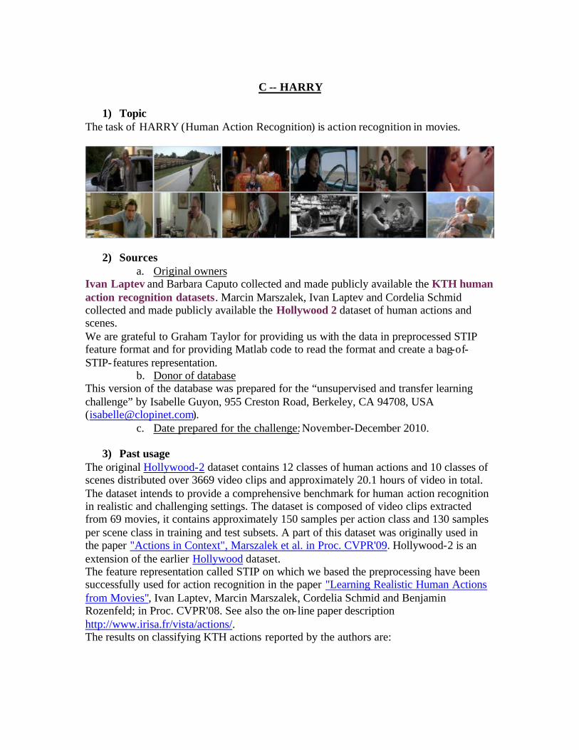
airplane: 4616 automobile: 4670 bird: 6000 cat: 6000 deer: 6000 dog: 6000 frog: 4630 horse: 4623 ship: 4658 truck: 4611 fruit_and_vegetables.apple: 600 fish.aquarium_fish: 600 people.baby: 600 large_carnivores.bear: 600 aquatic_mammals.beaver: 600 household_furniture.bed: 600 insects.bee: 600 insects.beetle: 600 vehicles_1.bicycle: 600 food_containers.bottle: 600 food_containers.bowl: 600 people.boy: 600 large_man-made_outdoor_things.bridge: 600 vehicles_1.bus: 600 insects.butterfly: 600 large_omnivores_and_herbivores.camel: 600 food_containers.can: 600 large_man-made_outdoor_things.castle: 600 insects.caterpillar: 600 large_omnivores_and_herbivores.cattle: 600 household_furniture.chair: 600 large_omnivores_and_herbivores.chimpanzee: 600 household_electrical_devices.clock: 600 large_natural_outdoor_scenes.cloud: 600 insects.cockroach: 600 household_furniture.couch: 600 non-insect_invertebrates.crab: 600 reptiles.crocodile: 600 food_containers.cup: 600 reptiles.dinosaur: 600 aquatic_mammals.dolphin: 600 large_omnivores_and_herbivores.elephant: 600 fish.flatfish: 600 large_natural_outdoor_scenes.forest: 600 medium_mammals.fox: 600 people.girl: 600 small_mammals.hamster: 600 large_man-made_outdoor_things.house: 600 large_omnivores_and_herbivores.kangaroo: 600 household_electrical_devices.keyboard: 600 household_electrical_devices.lamp: 600 vehicles_2.lawn_mower: 600

large_carnivores.leopard: 600 large_carnivores.lion: 600 reptiles.lizard: 600 non-insect_invertebrates.lobster: 600 people.man: 600 trees.maple_tree: 600 vehicles_1.motorcycle: 600 large_natural_outdoor_scenes.mountain: 600 small_mammals.mouse: 600 fruit_and_vegetables.mushroom: 600 trees.oak_tree: 600 fruit_and_vegetables.orange: 600 flowers.orchid: 600 aquatic_mammals.otter: 600 trees.palm_tree: 600 fruit_and_vegetables.pear: 600 vehicles_1.pickup_truck: 600 trees.pine_tree: 600 large_natural_outdoor_scenes.plain: 600 food_containers.plate: 600 flowers.poppy: 600 medium_mammals.porcupine: 600 medium_mammals.possum: 600 small_mammals.rabbit: 600 medium_mammals.raccoon: 600 fish.ray: 600 large_man-made_outdoor_things.road: 600 vehicles_2.rocket: 600 flowers.rose: 600 large_natural_outdoor_scenes.sea: 600 aquatic_mammals.seal: 600 fish.shark: 600 small_mammals.shrew: 600 medium_mammals.skunk: 600 large_man-made_outdoor_things.skyscraper: 600 non-insect_invertebrates.snail: 600 reptiles.snake: 600 non-insect_invertebrates.spider: 600 small_mammals.squirrel: 600 vehicles_2.streetcar: 600 flowers.sunflower: 600 fruit_and_vegetables.sweet_pepper: 600 household_furniture.table: 600 vehicles_2.tank: 600 household_electrical_devices.telephone: 600 household_electrical_devices.television: 600 large_carnivores.tiger: 600 vehicles_2.tractor: 600 vehicles_1.train: 600 fish.trout: 600 flowers.tulip: 600 reptiles.turtle: 600

household_furniture.wardrobe: 600 aquatic_mammals.whale: 600 trees.willow_tree: 600 large_carnivores.wolf: 600 people.woman: 600 non-insect_invertebrates.worm: 600 Transfer labels (24000 labels): bird: 6000 cat: 6000 deer: 6000 dog: 6000

6) Baseline results The data were preprocessed with kmeans clustering as described in Section A.

Table D2: Baseline results (normalized ALC for 64 training examples). RITA Valid Final Raw 0.2504 0.4133 Preprocessed 0.2417 0.3413

Figure D4: Baseline results on preprocessed data (top valid, bottom final).

E- SYLVESTER

1) Topic The task of SYLVESTER is to classify forest cover types. The task was carved out of data from the US Forest Service (USFS). The data include 7 labels corresponding to forest cover types. We used 2 for transfer learning (training), 2 for validation and 3 for testing.


Remote Sensing and GIS Program Department of Forest Sciences College of Natural Resources Colorado State University Fort Collins, CO 80523 (contact Jock A. Blackard, jblackard/[email protected] or Dr. Denis J. Dean, [email protected]) Jock A. Blackard USDA Forest Service 3825 E. Mulberry Fort Collins, CO 80524 USA jblackard/[email protected] Dr. Denis J. Dean Associate Professor Department of Forest Sciences Colorado State University Fort Collins, CO 80523 USA [email protected] Dr. Charles W. Anderson Associate Professor Department of Computer Science Colorado State University Fort Collins, CO 80523 USA [email protected] Acknowledgements, Copyright Information, and Availability Reuse of this database is unlimited with retention of copyright notice for Jock A. Blackard and Colorado State University.


c. Date received (original data): August 28, 1998, UCI Machine Learning Repository, under the name Forest Cover Type.

d. Date prepared for the challenge: September-November 2010.

3) Past usage

Blackard, Jock A. 1998. "Comparison of Neural Networks and Discriminant Analysis in Predicting Forest Cover Types." Ph.D. dissertation. Department of Forest Sciences. Colorado State University. Fort Collins, Colorado.

Classification performance with first 11,340 records used for training data, next 3,780 records used for validation data, and last 565,892 records used for testing data subset: -- 70% backpropagation -- 58% Linear Discriminant Analysis. The subtask SYLVA prepared for the “performance prediction challenge” and the “agnostic learning vs. prior knowledge” (ALvsPK) challenge is a 2-class classification problem (Ponderosa pine vs. others). The best results were obtained with Logitboost by Roman Lutz who obtained 0.4% error in the PK track and 0.6%error in the AL track. See http://clopinet.com/isabelle/Projects/agnostic/Results.html. The data were also used in the “active learning challenge” under the name “SYLVA” during the development phase and “F” (for FOREST) during the final test phase. The best entrants (Intel team) obtained a 0.8 area under the learning curve, see http://www.causality.inf.ethz.ch/activelearning.php?page=results.

4) Experimental design The original data comprises a total of 581012 instances (observations) grouped in 7 classes (forest cover types) and having 54 attributes (features) corresponding to 12 measures (10 quantitative variables, 4 binary wilderness areas and 40 binary soil type variables). The actual forest cover type for a given observation (30 x 30 meter cell) was determined from US Forest Service (USFS) Region 2 Resource Information System (RIS) data. Independent variables were derived from data originally obtained from US Geological Survey (USGS) and USFS data. Data is in raw form (not scaled) and contains binary (0 or 1) columns of data for qualitative independent variables (wilderness areas and soil types). Variable Information Given are the variable name, variable type, the measurement unit and a brief description. The forest cover type is the classification problem. The order of this listing corresponds to the order of numerals along the rows of the database. Name Data Type Measurement Description Elevation quantitative meters Elevation in meters Aspect quantitative azimuth Aspect in degrees azimuth Slope quantitative degrees Slope in degrees Horizontal_Distance_To_Hydrology quantitative meters Horz Dist to nearest surface water features Vertical_Distance_To_Hydrology quantitative meters Vert Dist to nearest surface water features Horizontal_Distance_To_Roadways quantitative meters Horz Dist to nearest roadway Hillshade_9am quantitative 0 to 255 index Hillshade index at 9am, summer solstice

Hillshade_Noon quantitative 0 to 255 index Hillshade index at noon, summer soltice Hillshade_3pm quantitative 0 to 255 index Hillshade index at 3pm, summer solstice Horizontal_Distance_To_Fire_Points quantitative meters Horz Dist to nearest wildfire ignition points Wilderness_Area (4 binary columns) qualitative 0 (absence) or 1 (presence) Wilderness area designation Soil_Type (40 binary columns) qualitative 0 (absence) or 1 (presence) Soil Type designation Cover_Type (7 types) integer 1 to 7 Forest Cover Type designation

Code Designations Wilderness Areas: 1 -- Rawah Wilderness Area 2 -- Neota Wilderness Area 3 -- Comanche Peak Wilderness Area 4 -- Cache la Poudre Wilderness Area Soil Types: 1 to 40 : based on the USFS Ecological Landtype Units for this study area. Forest Cover Types: 1 -- Spruce/Fir 2 -- Lodgepole Pine 3 -- Ponderosa Pine 4 -- Cottonwood/Willow 5 -- Aspen 6 -- Douglas-fir 7 – Krummholz Class Distribution Number of records of Spruce-Fir: 211840 Number of records of Lodgepole Pine: 283301 Number of records of Ponderosa Pine: 35754 Number of records of Cottonwood/Willow: 2747 Number of records of Aspen: 9493 Number of records of Douglas-fir: 17367 Number of records of Krummholz: 20510 Total records: 581012 Data preprocessing and data split We mixed mixed the classes to get approximately the same error rate in baseline results on the validation set and the final evaluation set. We used the original data encoding from the data donors, transformed by an invertible linear transform (an isometry). To make it even harder to go back to the original data, non- informative features (distractors) were added, corresponding to randomly permuted column values of the original features, before applying the isometry. We then randomized the order of the features and patterns. We quantized the values between 0 and 999.

5) Number of examples and class distribution Table E1: Statistics on the SYLVESTER data

Dataset Domain Feat. type

Feat. num.

Sparsity (%) Label

Development num.

Transfer num.

Validation num

Final eval. num.

SYLVESTER Ecology Numeric 100 0 Binary 572820 10000 4096 4096

There are no missing values. Here is class label composition of the data subsets: Validation set: X[4096, 100] Y[4096, 1] Ponderosa Pine: 2044 Aspen: 2052 Final set: X[4096, 100] Y[4096, 1] Spruce/Fir: 1319 Douglas-fir: 1404 Krummholz: 1373 Development set: X[572820, 100] Y[572820, 1] Spruce/Fir: 210521 Lodgepole Pine: 283301 Ponderosa Pine: 33710 Cottonwood/Willow: 2747 Aspen: 7441 Douglas-fir: 15963 Krummholz: 19137 Transfer labels (10000 labels): Lodgepole Pine: 9891 Cottonwood/Willow: 109

6) Type of input variables and variable statistics 100 numeric variables transformed via a random isometry from the raw input variables to which 46 distractors were added. The distractors were obtained by picking real variables and randomizing the order of the values. The final variables were quantized between 0 and 999.

7) Baseline results We show results using our baseline classifier shown in appendix. The prepreprocessing in kmeans clustering (20 clusters). Table E2: Baseline results (normalized ALC for 64 training examples).

SYLVESTER Valid Final Raw 0.2167 0.3095 Preprocessed 0.1670 0.2362

Figure E1: Baseline results on raw data (top valid, bottom final).

F -- TERRY

1) Topic The task of TERRY is the Text Recognition dataset.


The data were donated by Reuters and downloaded from: Lewis, D. D. RCV1-v2/LYRL2004: The LYRL2004 Distribution of the RCV1-v2 Text Categorization Test Collection (12-Apr-2004 Version). http://www.jmlr.org/papers/volume5/lewis04a/lyrl2004_rcv1v2_README.htm.


c. Date prepared for the challenge: November-December 2010.

3) Past usage Lewis, D. D.; Yang, Y.; Rose, T.; and Li, F. RCV1: A New Benchmark Collection for Text Categorization Research. Journal of Machine Learning Research, 5:361-397, 2004. http://www.jmlr.org/papers/volume5/lewis04a/lewis04a.pdf.

4) Experimental design We used a subset of the 800,000 documents of the RCV1-v2 data collection, formatted in a bag-of-words representation. The representation uses 47,236 unique stemmed tokens. The representation was obtained from on-line appendix B.13. The list of stems was found in on- line appendix B14. We used as target values the topic categories (on- line appendices 3 and 8). We considered all levels of the hierarchy to select the most promising categories. The features were obfuscated by making a non- linear transformation of the values then quantizing them between 0 and 999. Further, the raws and lines of the data matrix were permuted.

5) Data statistics

Table C1: Data statistics for TERRY


Sparsity (%)

Development num.

Transfer num.

Validation num

Final eval. num.

TERRY Text recognition 47236 99.84 217034 40000 4096 4096

All variables are numeric (no categorical variable). There are no missing values. The target variables are categorical. The data are very sparse, so they were stored in a sparse matrix. Here is class label composition of the data subsets: Validation set: X[4096, 47236] Y[4096, 5] ENERGY MARKETS: 808

EUROPEAN COMMUNITY: 886 PRIVATISATIONS: 817 MANAGEMENT: 863 ENVIRONMENT AND NATURAL WORLD: 826 Final set: X[4096, 47236] Y[4096, 5] SPORTS: 797 CREDIT RATINGS: 804 DISASTERS AND ACCIDENTS: 829 ELECTIONS: 856 LABOUR ISSUES: 829 Development set: X[217034, 47236] Y[217034, 103] STRATEGY/PLANS: 6944 LEGAL/JUDICIAL: 2898 REGULATION/POLICY: 10279 SHARE LISTINGS: 2166 PERFORMANCE: 42290 ACCOUNTS/EARNINGS: 21832 ANNUAL RESULTS: 2243 COMMENT/FORECASTS: 21315 INSOLVENCY/LIQUIDITY: 494 FUNDING/CAPITAL: 11885 SHARE CAPITAL: 5378 BONDS/DEBT ISSUES: 3147 LOANS/CREDITS: 705 CREDIT RATINGS: 1453 OWNERSHIP CHANGES: 13853 MERGERS/ACQUISITIONS: 11739 ASSET TRANSFERS: 1312 PRIVATISATIONS: 1370 PRODUCTION/SERVICES: 7749 NEW PRODUCTS/SERVICES: 1967 RESEARCH/DEVELOPMENT: 751 CAPACITY/FACILITIES: 8895 MARKETS/MARKETING: 11832 DOMESTIC MARKETS: 1199 EXTERNAL MARKETS: 1999 MARKET SHARE: 282 ADVERTISING/PROMOTION: 513 CONTRACTS/ORDERS: 4360 DEFENCE CONTRACTS: 339 MONOPOLIES/COMPETITION: 1264 MANAGEMENT: 2245 MANAGEMENT MOVES: 2044 LABOUR: 2971 CORPORATE/INDUSTRIAL: 105241 ECONOMIC PERFORMANCE: 2462 MONETARY/ECONOMIC: 7044 MONEY SUPPLY: 632 INFLATION/PRICES: 1924 CONSUMER PRICES: 1642

WHOLESALE PRICES: 288 CONSUMER FINANCE: 615 PERSONAL INCOME: 84 CONSUMER CREDIT: 63 RETAIL SALES: 365 GOVERNMENT FINANCE: 12008 EXPENDITURE/REVENUE: 4066 GOVERNMENT BORROWING: 8052 OUTPUT/CAPACITY: 679 INDUSTRIAL PRODUCTION: 482 CAPACITY UTILIZATION: 13 INVENTORIES: 30 EMPLOYMENT/LABOUR: 4087 UNEMPLOYMENT: 484 TRADE/RESERVES: 6412 BALANCE OF PAYMENTS: 933 MERCHANDISE TRADE: 3994 RESERVES: 546 HOUSING STARTS: 104 LEADING INDICATORS: 1556 ECONOMICS: 33239 EUROPEAN COMMUNITY: 5554 EC INTERNAL MARKET: 945 EC CORPORATE POLICY: 559 EC AGRICULTURE POLICY: 620 EC MONETARY/ECONOMIC: 2219 EC INSTITUTIONS: 561 EC ENVIRONMENT ISSUES: 50 EC COMPETITION/SUBSIDY: 524 EC EXTERNAL RELATIONS: 1142 EC GENERAL: 18 GOVERNMENT/SOCIAL: 63881 CRIME, LAW ENFORCEMENT: 8380 DEFENCE: 2506 INTERNATIONAL RELATIONS: 11105 DISASTERS AND ACCIDENTS: 1488 ARTS, CULTURE, ENTERTAINMENT: 1078 ENVIRONMENT AND NATURAL WORLD: 790 FASHION: 76 HEALTH: 1744 LABOUR ISSUES: 4161 OBITUARIES: 184 HUMAN INTEREST: 667 DOMESTIC POLITICS: 15654 BIOGRAPHIES, PERSONALITIES, PEOPLE: 1668 RELIGION: 804 SCIENCE AND TECHNOLOGY: 638 SPORTS: 8671 TRAVEL AND TOURISM: 223 WAR, CIVIL WAR: 9323 ELECTIONS: 3539 WEATHER: 821

WELFARE, SOCIAL SERVICES: 484 EQUITY MARKETS: 12424 BOND MARKETS: 6179 MONEY MARKETS: 13574 INTERBANK MARKETS: 7279 FOREX MARKETS: 6599 COMMODITY MARKETS: 21557 SOFT COMMODITIES: 12155 METALS TRADING: 3092 ENERGY MARKETS: 5162 MARKETS: 51279 Transfer labels (40000 labels): DOMESTIC POLITICS: 12865 MONEY MARKETS: 11322 REGULATION/POLICY: 8508 GOVERNMENT FINANCE: 9900

6) Baseline results

The data were preprocessed with kmeans clustering as described in Section A.

Table C2: Baseline results (normalized ALC for 64 training examples). TERRY Valid Final Raw 0.6969 0.7550 Preprocessed 0.6602 0.3440

We see in Table C2 and Figure C1 that the performances in preprocessed data in the final evaluation set are not good. This is another example of preprocessing overfiting: we used the clusters found with the validation set to preprocess the test set.

Figure B1: Baseline results on preprocessed data (top valid, bottom final).

Appendix Code for the linear classifier function [data, model]=train(model, data) %[data, model]=train(model, data) % Simple linear classifier with Hebbian-style learning. % Inputs: % model -- A hebbian learning object. % data -- A data object. % Returns: % model -- The trained model. % data -- A new data structure containing the results. % Usually works best with standardized data. Standardization is not % performed here for computational reasons (we put it outside the CV loop). % Isabelle Guyon -- [email protected] -- November 2010 if model.verbosity>0, fprintf('==> Training Hebbian classifier ... '); end Posidx=find(data.Y>0); Negidx=find(data.Y<0); if pd_check(data) % Kernelized version model.W=zeros(1, length(data.Y)); model.W(Posidx)=1/(length(Posidx)+eps); model.W(Negidx)=-1/(length(Negidx)+eps); else n=size(data.X, 2); Mu1=zeros(1, n); Mu2=zeros(1, n); if ~isempty(Posidx) Mu1=mean(data.X(Posidx,:), 1); end if ~isempty(Negidx) Mu2=mean(data.X(Negidx,:), 1); end model.W=Mu1-Mu2; B=(Mu1+Mu2)/2; model.b0=-model.W*B'; end % Test the model if model.test_on_training_data data=test(model, data); end if model.verbosity>0, fprintf('done\n'); end

Datasets of the Unsupervised and Transfer Learning Challenge · Datasets of the Unsupervised and...

Documents

Transcript of Datasets of the Unsupervised and Transfer Learning Challenge · Datasets of the Unsupervised and...