Data$Mining$MTAT.03.183$ … · – Hector Garcia-Molina, Stanford University ... " snowflake...
94
Data Mining MTAT.03.183 Online Analy4cal Processing and Data Warehouses Jaak Vilo 2011 Fall
Transcript of Data$Mining$MTAT.03.183$ … · – Hector Garcia-Molina, Stanford University ... " snowflake...
Data Mining MTAT.03.183
Online Analy4cal Processing and Data Warehouses
Jaak Vilo 2011 Fall
Acknowledgment • This slide deck is a “mashup” of the
following publicly available slide decks: – http://www.postech.ac.kr/~swhwang/grass/DataCube.ppt – http://classweb.gmu.edu/kersch/inft864/Readings/Shoshani/
DataCube/CubeNotesKerschberg.ppt – http://ohr.gsfc.nasa.gov/wfstatistics/Data_Cube_Training.ppt – http://www.cs.uiuc.edu/homes/hanj/bk2/03.ppt – Hector Garcia-Molina, Stanford University – Marlon Dumas, Univ. of Tartu, – Sulev Reisberg, Quretec & STACC
– …

Outline
• The “data cube” abstraction • Multidimensional data models • Data warehouses
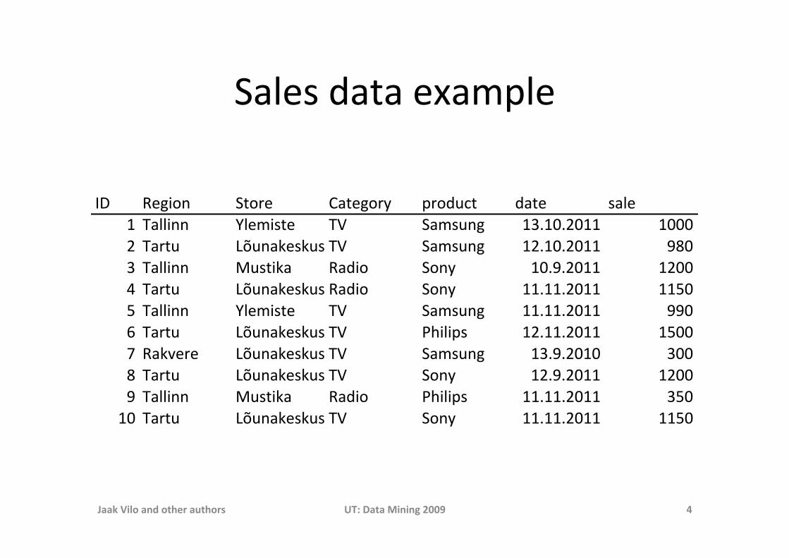
Sales data example
!" #$%&'( )*'+$ ,-*$%'+. /+'012* 0-*$ 3-4$5 6-44&(( 74$8&3*$ 69 )-831(% 5:;5<;=<55 5<<<= 6-+*1 >?1(-@$3@13 69 )-831(% 5=;5<;=<55 AB<: 6-44&(( C13*&@- #-0&' )'(. 5<;A;=<55 5=<<D 6-+*1 >?1(-@$3@13 #-0&' )'(. 55;55;=<55 55E<E 6-44&(( 74$8&3*$ 69 )-831(% 55;55;=<55 AA<F 6-+*1 >?1(-@$3@13 69 GH&4&/3 5=;55;=<55 5E<<I #-@J$+$ >?1(-@$3@13 69 )-831(% 5:;A;=<5< :<<B 6-+*1 >?1(-@$3@13 69 )'(. 5=;A;=<55 5=<<A 6-44&(( C13*&@- #-0&' GH&4&/3 55;55;=<55 :E<5< 6-+*1 >?1(-@$3@13 69 )'(. 55;55;=<55 55E<
Jaak Vilo and other authors UT: Data Mining 2009 4
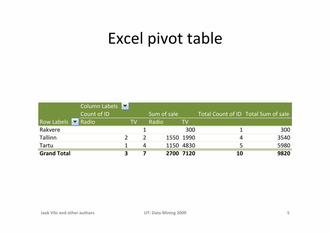
Excel pivot table
!"#$%&'()*+#,!"$&-'".'/0 1$%'".',)#+ 2"-)#'!"$&-'".'/0 2"-)#'1$%'".',)#+
3"4'()*+#, 3)56" 27 3)56" 273)89+:+ ; <== ; <==2)##6&& > > ;??= ;@@= A <?A=2):-$ ; A ;;?= AB<= ? ?@B=!"#$%&'()#* + , -,.. ,/-. /. 01-.
Jaak Vilo and other authors UT: Data Mining 2009 5

Example: Sales
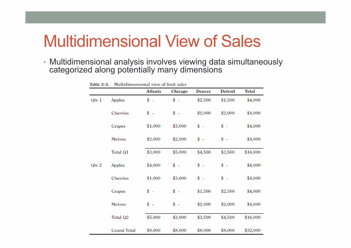
Multidimensional View of Sales • Multidimensional analysis involves viewing data simultaneously
categorized along potentially many dimensions
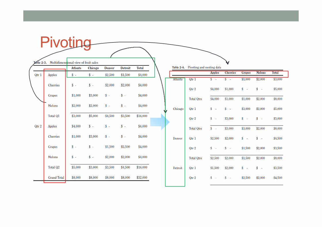
Pivoting

Typical Data Analysis Process
• Formulate a query to extract relevant information • Extract aggregated data from the database • Visualize the result to look for patterns. • Analyze the result and formulate new queries. • Online Analytical Processing (OLAP) is about
supporting such processes • OLAP characteristics: No updates, lots of
aggregation, need to visualize and to interact • Let’s first talk about aggregation…
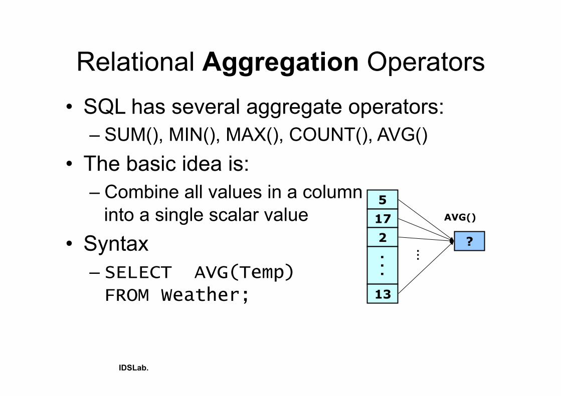
Relational Aggregation Operators • SQL has several aggregate operators:
– SUM(), MIN(), MAX(), COUNT(), AVG() • The basic idea is:
– Combine all values in a column into a single scalar value
• Syntax – SELECT AVG(Temp) FROM Weather;
IDSLab.
5 17 2
. . .
13
? …
AVG()
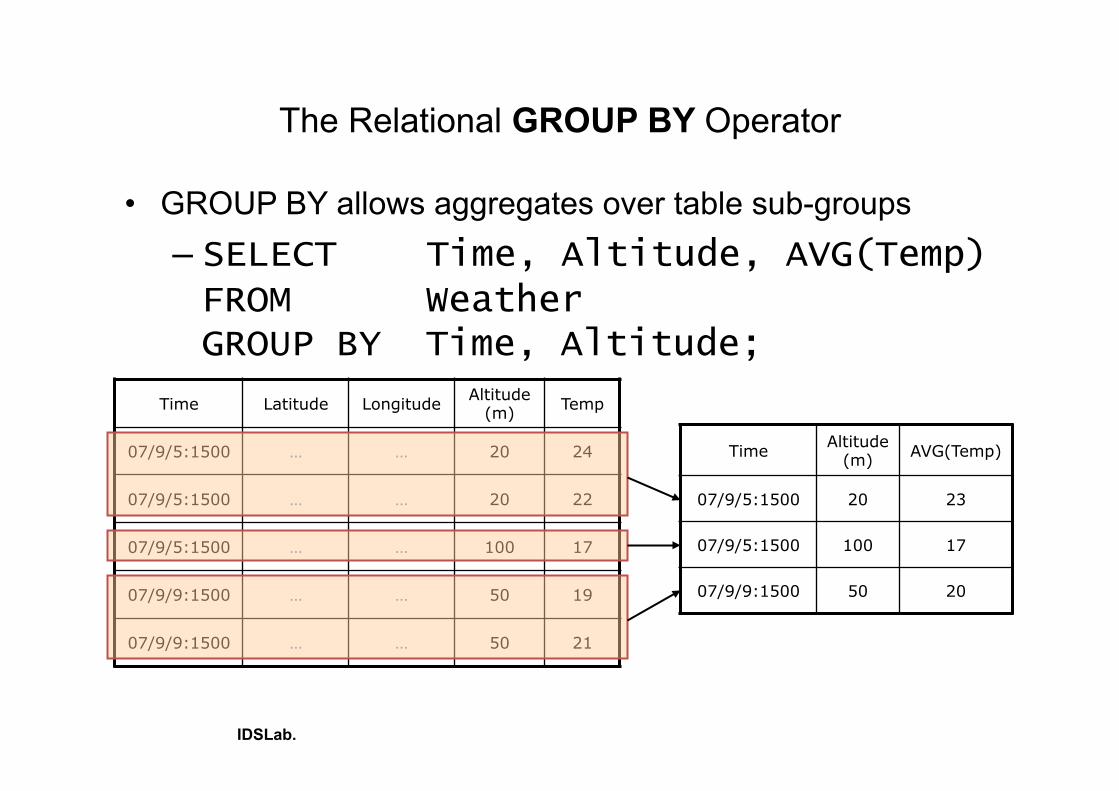
The Relational GROUP BY Operator
• GROUP BY allows aggregates over table sub-groups – SELECT Time, Altitude, AVG(Temp) FROM Weather GROUP BY Time, Altitude;
IDSLab.
Time Latitude Longitude Altitude (m) Temp
07/9/5:1500 … … 20 24
07/9/5:1500 … … 20 22
07/9/5:1500 … … 100 17
07/9/9:1500 … … 50 19
07/9/9:1500 … … 50 21
Time Altitude (m) AVG(Temp)
07/9/5:1500 20 23
07/9/5:1500 100 17
07/9/9:1500 50 20
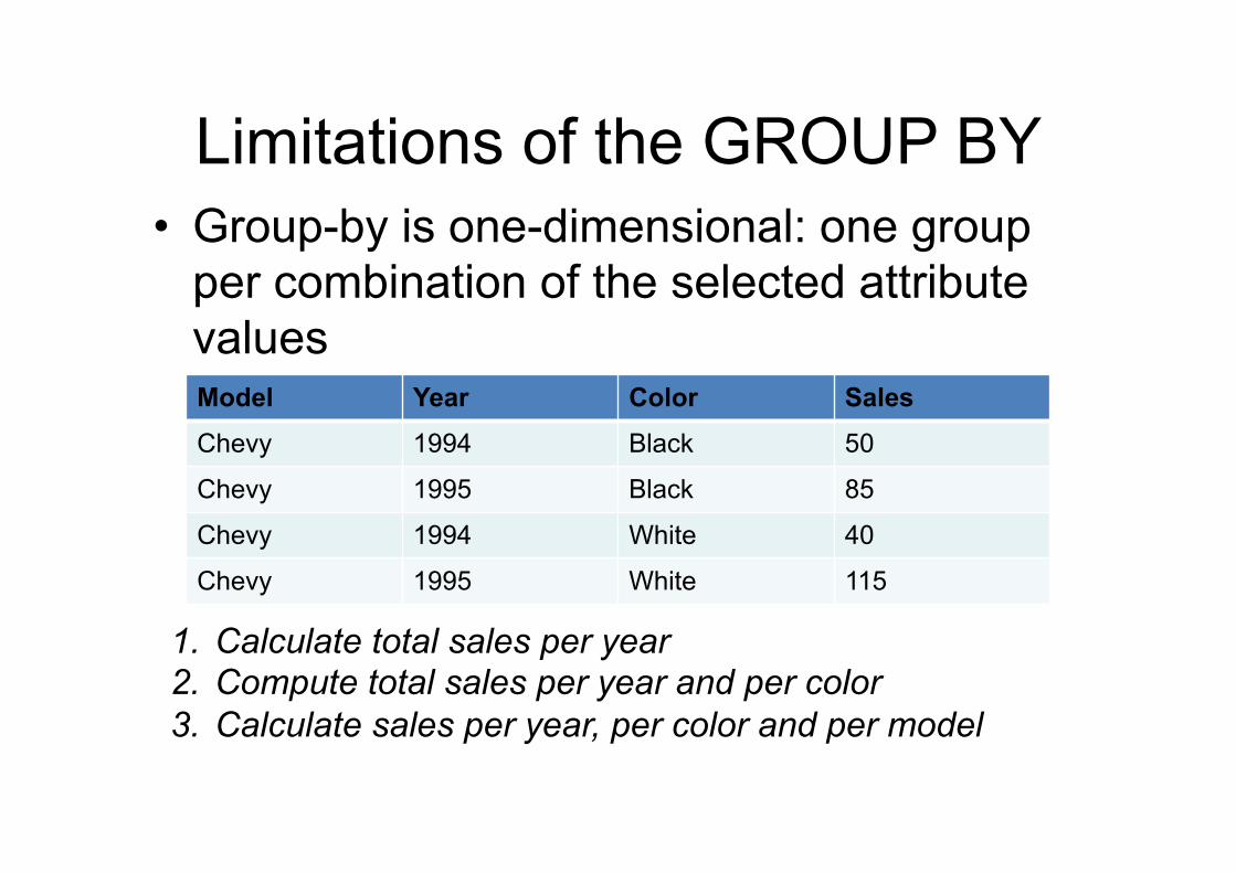
Limitations of the GROUP BY • Group-by is one-dimensional: one group
per combination of the selected attribute values à Does not give sub-totals Model Year Color Sales
Chevy 1994 Black 50
Chevy 1995 Black 85
Chevy 1994 White 40
Chevy 1995 White 115
1. Calculate total sales per year 2. Compute total sales per year and per color 3. Calculate sales per year, per color and per model
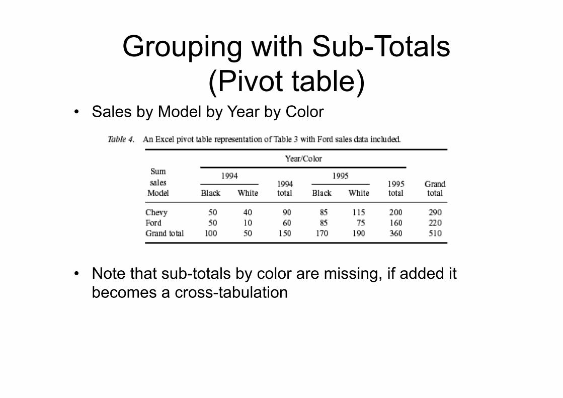
Grouping with Sub-Totals (Pivot table)
• Sales by Model by Year by Color
• Note that sub-totals by color are missing, if added it
becomes a cross-tabulation

Grouping with sub-totals (cross-tab)

Grouping with Sub-Totals (Relational version)
IDSLab.
Sub-totals by color are still missing…
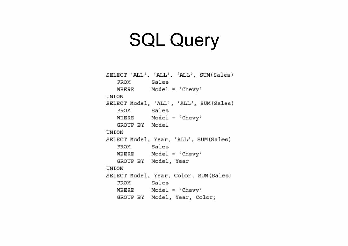
SQL Query

17
Adding the colors…
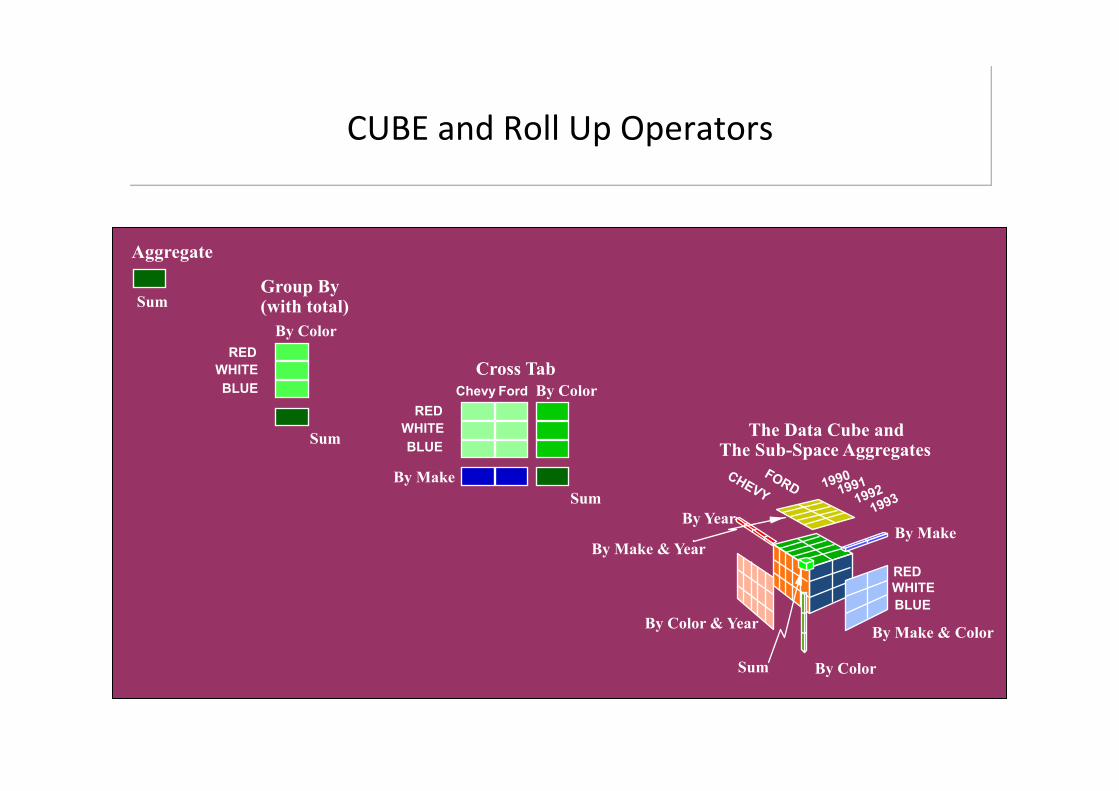
CUBE and Roll Up Operators
1990 1991
RED WHITE BLUE
By Color
By Make & Color
By Make & Year
By Color & Year
By Make By Year
Sum
The Data Cube and The Sub-Space Aggregates
RED WHITE BLUE
Chevy Ford
By Make
By Color
Sum
Cross Tab RED
WHITE BLUE
By Color
Sum
Group By (with total) Sum
Aggregate

The Cube • An Example of 3D Data Cube
IDSLab. 19
By Year By Make
By Color
Sum
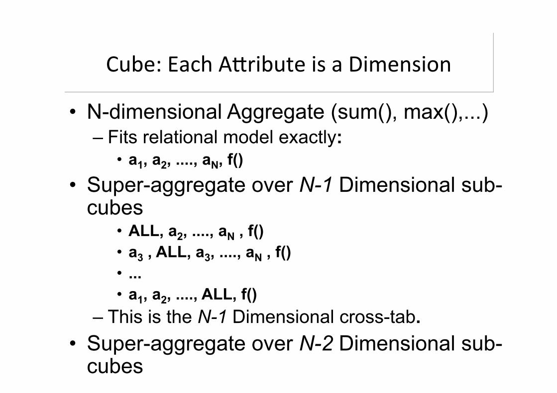
Cube: Each ADribute is a Dimension
• N-dimensional Aggregate (sum(), max(),...) – Fits relational model exactly:
• a1, a2, ...., aN, f() • Super-aggregate over N-1 Dimensional sub-
cubes • ALL, a2, ...., aN , f() • a3 , ALL, a3, ...., aN , f() • ... • a1, a2, ...., ALL, f()
– This is the N-1 Dimensional cross-tab. • Super-aggregate over N-2 Dimensional sub-
cubes • ALL, ALL, a3, ...., aN , f() • ... • a1, a2 ,...., ALL, ALL, f()
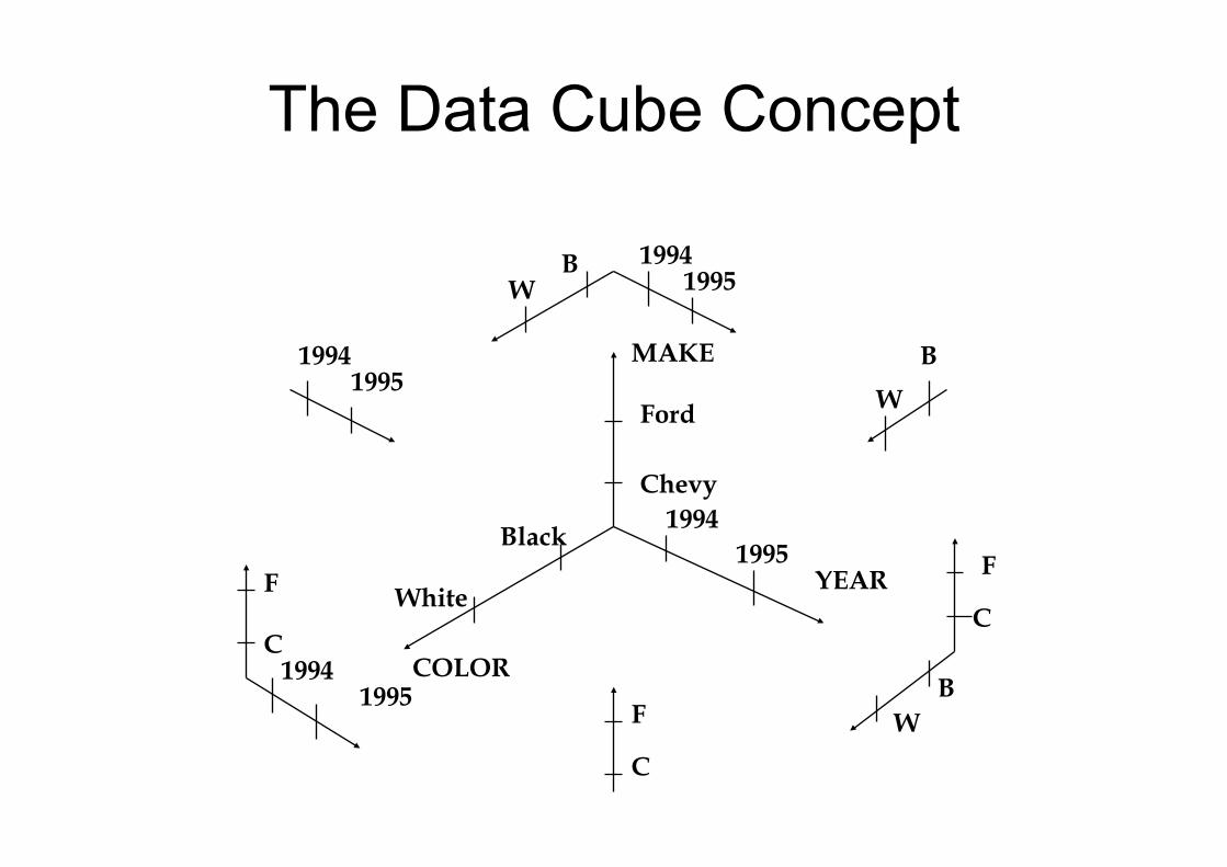
The Data Cube Concept
MAKE
YEAR
COLOR
Ford
Chevy
Black
White
1994 1995
1994 1995
B
W
C
F
F
C
B W
F
C 1994
1995
B W
1994 1995

Sub-cube Derivation
• Dimension collapse, * denotes ALL
<M,Y,C>
<M,Y,*> <M,*,C> <*,Y,C>
<M,*,*> <*,Y,*> <*,*,C>
<*,*,*>

23 IDSLab. 23
CUBE Operator Possible syntax
• Proposed syntax example: – SELECT Model, Make, Year, SUM(Sales) FROM Sales WHERE Model IN {“Chevy”, “Ford”} AND Year BETWEEN 1990 AND 1994 GROUP BY CUBE Model, Make, Year HAVING SUM(Sales) > 0;
– Note: GROUP BY operator repeats aggregate list • in select list • in group by list
24 IDSLab.
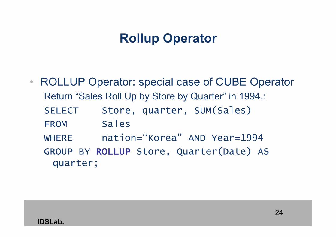
Rollup Operator
• ROLLUP Operator: special case of CUBE Operator Return “Sales Roll Up by Store by Quarter” in 1994.: SELECT Store, quarter, SUM(Sales)
FROM Sales
WHERE nation=“Korea” AND Year=1994
GROUP BY ROLLUP Store, Quarter(Date) AS quarter;

25
Cube Operator Example
SALES Model Year Color Sales Chevy 1990 red 5 Chevy 1990 white 87 Chevy 1990 blue 62 Chevy 1991 red 54 Chevy 1991 white 95 Chevy 1991 blue 49 Chevy 1992 red 31 Chevy 1992 white 54 Chevy 1992 blue 71 Ford 1990 red 64 Ford 1990 white 62 Ford 1990 blue 63 Ford 1991 red 52 Ford 1991 white 9 Ford 1991 blue 55 Ford 1992 red 27 Ford 1992 white 62 Ford 1992 blue 39
DATA CUBE Model Year Color Sales ALL ALL ALL 942 chevy ALL ALL 510 ford ALL ALL 432 ALL 1990 ALL 343 ALL 1991 ALL 314 ALL 1992 ALL 285 ALL ALL red 165 ALL ALL white 273 ALL ALL blue 339 chevy 1990 ALL 154 chevy 1991 ALL 199 chevy 1992 ALL 157 ford 1990 ALL 189 ford 1991 ALL 116 ford 1992 ALL 128 chevy ALL red 91 chevy ALL white 236 chevy ALL blue 183 ford ALL red 144 ford ALL white 133 ford ALL blue 156 ALL 1990 red 69 ALL 1990 white 149 ALL 1990 blue 125 ALL 1991 red 107 ALL 1991 white 104 ALL 1991 blue 104 ALL 1992 red 59 ALL 1992 white 116 ALL 1992 blue 110
CUBE
26 IDSLab. 26
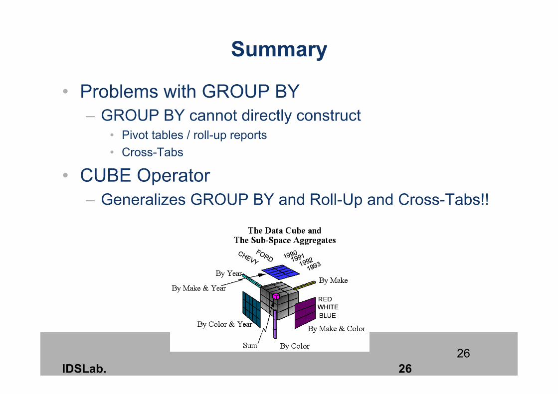
Summary
• Problems with GROUP BY – GROUP BY cannot directly construct
• Pivot tables / roll-up reports • Cross-Tabs
• CUBE Operator – Generalizes GROUP BY and Roll-Up and Cross-Tabs!!
27
Now let’s have a look at one…
• NASA Workforce cubes http://nasapeople.nasa.gov/workforce
• Btell demo reports – http://www.btell.de – Follow the “demo” link and start a demo, the go to
reports

OLAP Screen Example
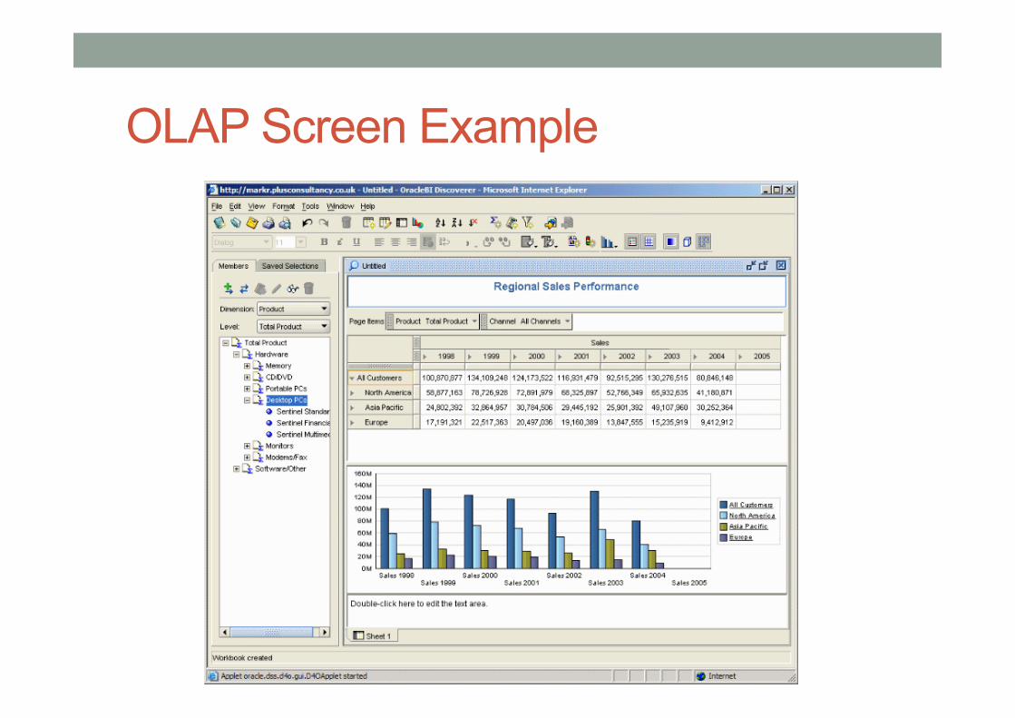
OLAP Screen Example
Hector Garcia Molina: Data Warehousing and OLAP 30
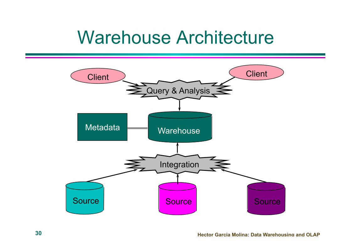
Warehouse Architecture
Client Client
Warehouse
Source Source Source
Query & Analysis
Integration
Metadata

Hector Garcia Molina: Data Warehousing and OLAP 31
Why a Warehouse?
Two Approaches: Query-Driven (Lazy) Warehouse (Eager)
Source Source
?

32
Multidimensional Data
• Sales volume as a function of product, month, and region
Prod
uct
Dimensions: Product, Location, Time Hierarchical summarization paths
Industry Region Year Category Country Quarter Product City Month Week Office Day
J. Han: Data Mining: Concepts and Techniques
Hector Garcia Molina: Data Warehousing and OLAP 33
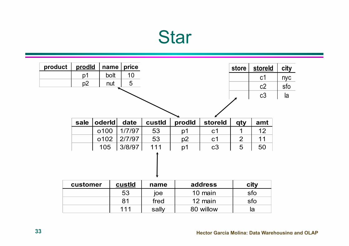
Star
customer custId name address city53 joe 10 main sfo81 fred 12 main sfo
111 sally 80 willow la
product prodId name pricep1 bolt 10p2 nut 5
store storeId cityc1 nycc2 sfoc3 la
sale oderId date custId prodId storeId qty amto100 1/7/97 53 p1 c1 1 12o102 2/7/97 53 p2 c1 2 11105 3/8/97 111 p1 c3 5 50
Hector Garcia Molina: Data Warehousing and OLAP 34
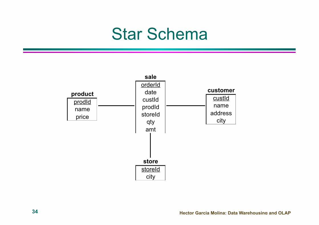
Star Schema
saleorderIddatecustIdprodIdstoreIdqtyamt
customercustIdnameaddresscity
productprodIdnameprice
storestoreIdcity
Hector Garcia Molina: Data Warehousing and OLAP 35
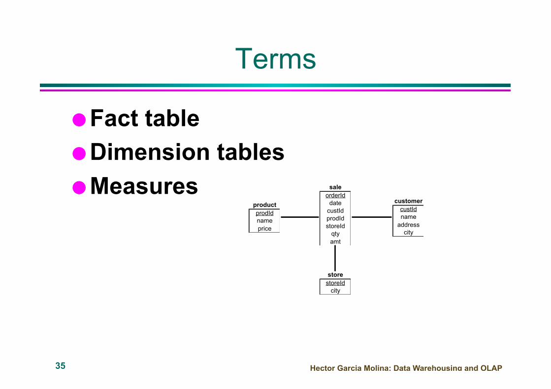
Terms
Fact table Dimension tables Measures sale
orderIddatecustIdprodIdstoreIdqtyamt
customercustIdnameaddresscity
productprodIdnameprice
storestoreIdcity
Hector Garcia Molina: Data Warehousing and OLAP 36
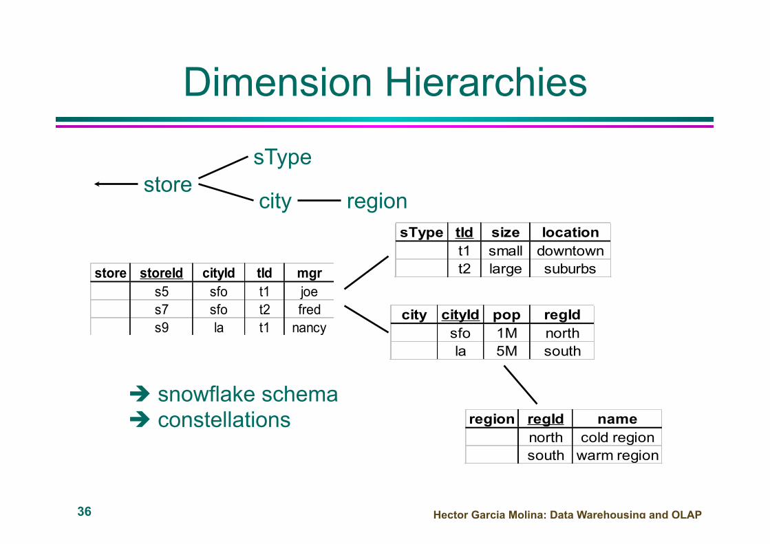
Dimension Hierarchies
store storeId cityId tId mgrs5 sfo t1 joes7 sfo t2 freds9 la t1 nancy
city cityId pop regIdsfo 1M northla 5M south
region regId namenorth cold regionsouth warm region
sType tId size locationt1 small downtownt2 large suburbs
store sType
city region
è snowflake schema è constellations

Hector Garcia Molina: Data Warehousing and OLAP 37
Cube
sale prodId storeId amtp1 c1 12p2 c1 11p1 c3 50p2 c2 8
c1 c2 c3p1 12 50p2 11 8
Fact table view: Multi-dimensional cube:
dimensions = 2

Hector Garcia Molina: Data Warehousing and OLAP 38
3-D Cube
sale prodId storeId date amtp1 c1 1 12p2 c1 1 11p1 c3 1 50p2 c2 1 8p1 c1 2 44p1 c2 2 4
day 2 c1 c2 c3p1 44 4p2 c1 c2 c3
p1 12 50p2 11 8
day 1
dimensions = 3
Multi-dimensional cube: Fact table view:
39
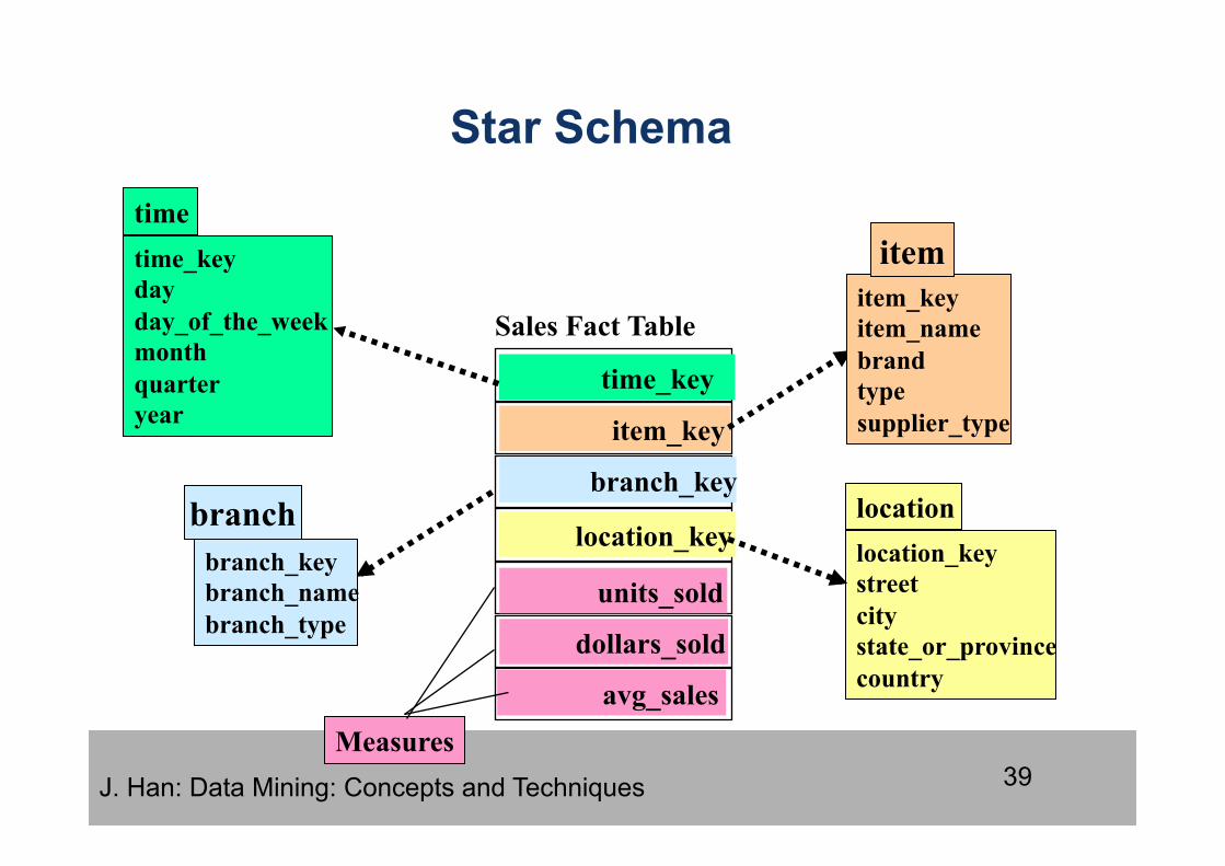
Star Schema
time_key day day_of_the_week month quarter year
time
location_key street city state_or_province country
location
Sales Fact Table
time_key
item_key
branch_key
location_key
units_sold
dollars_sold
avg_sales Measures
item_key item_name brand type supplier_type
item
branch_key branch_name branch_type
branch
J. Han: Data Mining: Concepts and Techniques
40
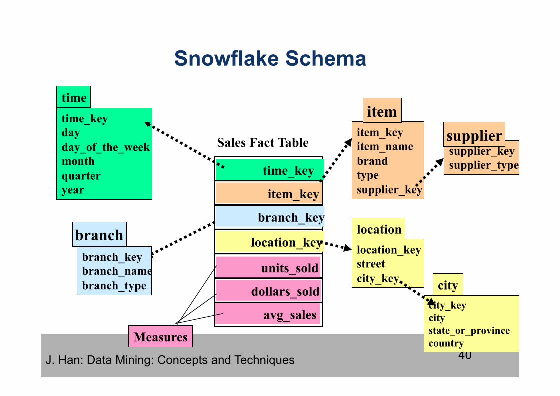
Snowflake Schema
time_key day day_of_the_week month quarter year
time
location_key street city_key
location
Sales Fact Table
time_key
item_key
branch_key
location_key
units_sold
dollars_sold
avg_sales
Measures
item_key item_name brand type supplier_key
item
branch_key branch_name branch_type
branch
supplier_key supplier_type
supplier
city_key city state_or_province country
city
J. Han: Data Mining: Concepts and Techniques
41
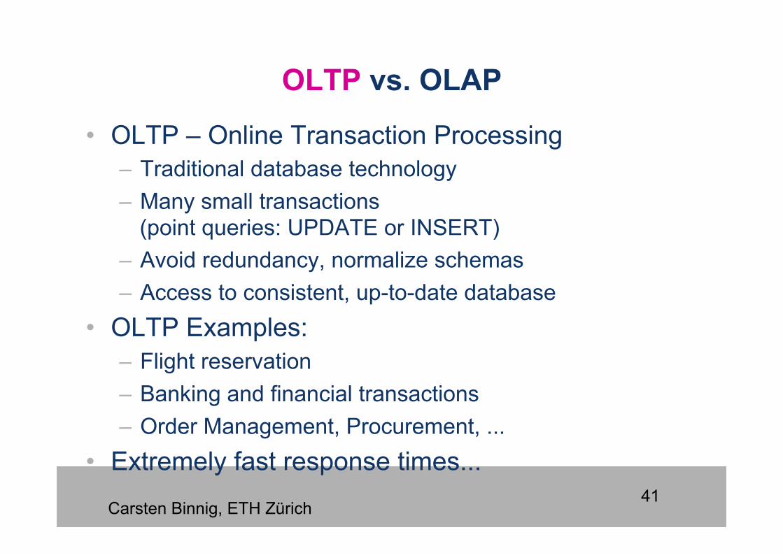
OLTP vs. OLAP
• OLTP – Online Transaction Processing – Traditional database technology – Many small transactions
(point queries: UPDATE or INSERT) – Avoid redundancy, normalize schemas – Access to consistent, up-to-date database
• OLTP Examples: – Flight reservation – Banking and financial transactions – Order Management, Procurement, ...
• Extremely fast response times...
Carsten Binnig, ETH Zürich

42
OLTP vs. OLAP
• OLAP – Online Analytical Processing – Big aggerate queries, no Updates – Redundancy a necessity (Materialized Views, special-
purpose indexes, de-normalized schemas) – Periodic refresh of data (daily or weekly)
• OLAP Examples – Decision support (sales per employee) – Marketing (purchases per customer) – Biomedical databases
• Goal: Response Time of seconds / few minutes
Carsten Binnig, ETH Zürich
43
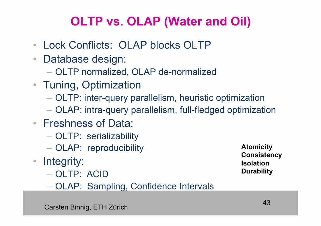
OLTP vs. OLAP (Water and Oil)
• Lock Conflicts: OLAP blocks OLTP • Database design:
– OLTP normalized, OLAP de-normalized • Tuning, Optimization
– OLTP: inter-query parallelism, heuristic optimization – OLAP: intra-query parallelism, full-fledged optimization
• Freshness of Data: – OLTP: serializability – OLAP: reproducibility
• Integrity: – OLTP: ACID – OLAP: Sampling, Confidence Intervals
Carsten Binnig, ETH Zürich
Atomicity Consistency Isolation Durability
44
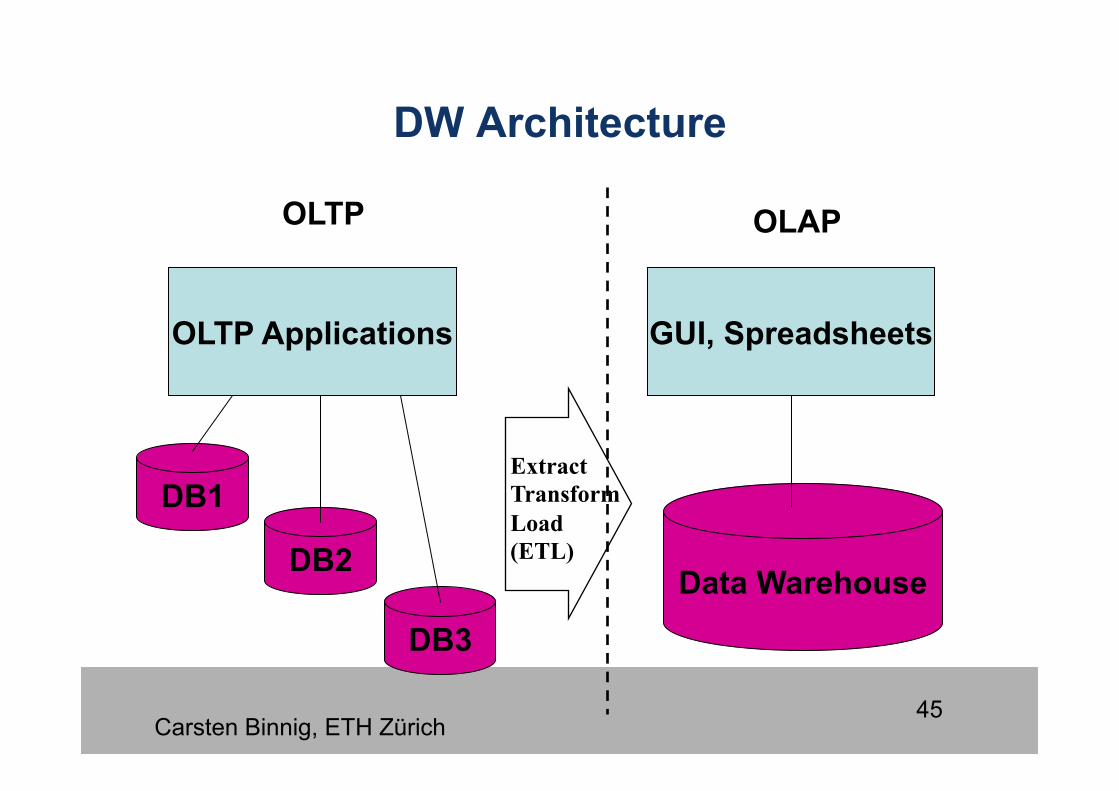
Solution: Data Warehouse
• Special Sandbox for OLAP • Data input using OLTP systems • Data Warehouse aggregates and replicates data
(special schema) • New Data is periodically uploaded to Warehouse
Carsten Binnig, ETH Zürich
45
DW Architecture
OLTP Applications GUI, Spreadsheets
DB1
DB2
DB3
Data Warehouse
OLTP OLAP
Carsten Binnig, ETH Zürich
Extract Transform Load (ETL)
What is data warehouse • InformaKon system for reporKng purposes • The goal is to fulfill reporKng needs which are unsaKsfied in operaKonal system • It is easy to modify old and design new reports
• No „write spec to soRware developer to get the report“ anymore
• Reports can be filled with data quickly • No „start the report generaKon at night to prevent system load“ anymore
• The data comes from operaKonal system(s)
Goal of the work package
• Work out the main concepts for building data warehouse for hospital IS • What are the reporKng needs? • What are the data cubes that cover most reporKng needs for „universal“ hospital?
• How to get the data into these cubes?
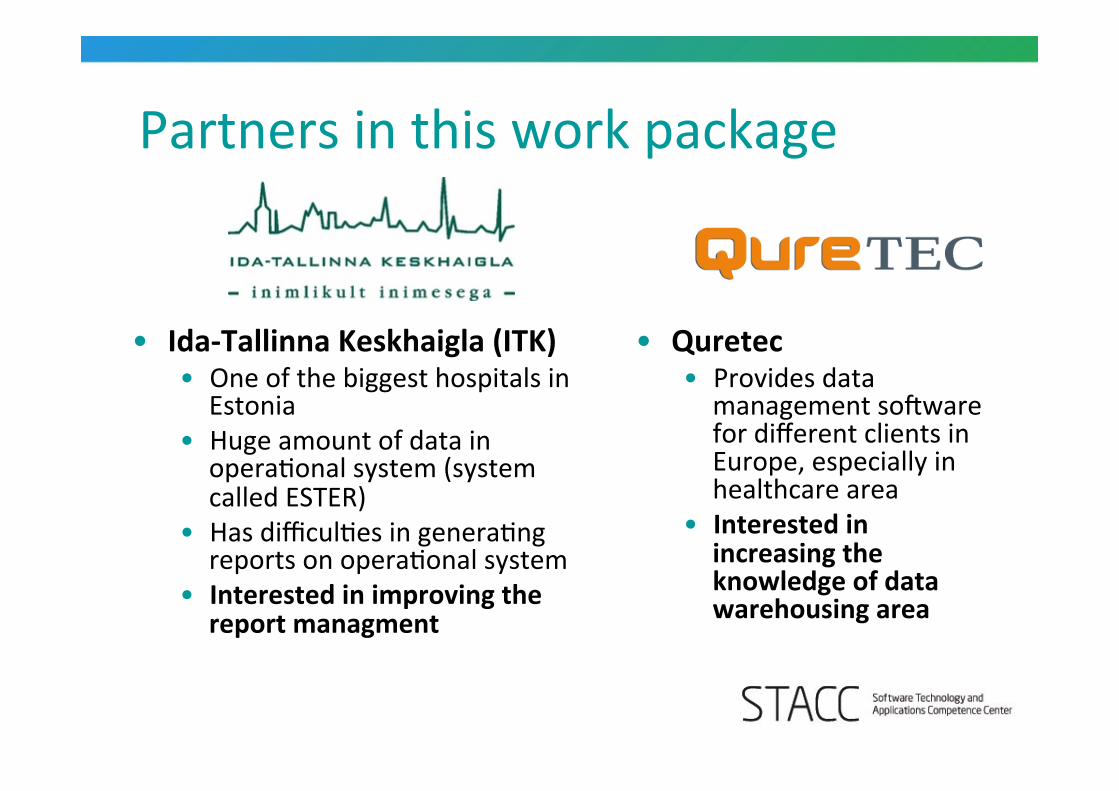
Partners in this work package
• Ida-‐Tallinna Keskhaigla (ITK) • One of the biggest hospitals in Estonia
• Huge amount of data in operaKonal system (system called ESTER)
• Has difficulKes in generaKng reports on operaKonal system
• Interested in improving the report managment
• Quretec • Provides data management soRware for different clients in Europe, especially in healthcare area
• Interested in increasing the knowledge of data warehousing area

So far... (1)
• We have analyzed the data and data structures in operaKonal system

So far...(2)
• We have designed the interface for ge`ng the data from ESTER
• We have built 2 data cubes
OperaKonal IS
SQL view
„Interface“ for building data
cubes Data cubes
Reports Data in operaKonal
IS
SQL view
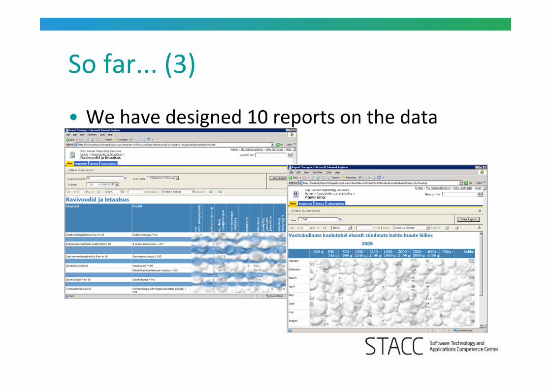
So far... (3)
• We have designed 10 reports on the data cubes
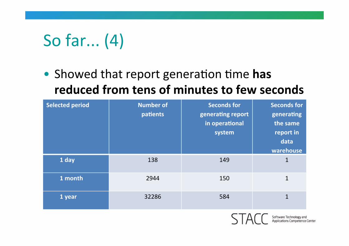
So far... (4)
• Showed that report generaKon Kme has reduced from tens of minutes to few seconds
Selected period Number of pa4ents
Seconds for genera4ng report in opera4onal
system
Seconds for genera4ng the same report in data
warehouse 1 day 138 149 1
1 month 2944 150 1
1 year 32286 584 1

So far... (5)
• We showed that data warehouse offers addiKonal benefits: • MulKple output formats • Reports can be redesigned easily • New combined reports -‐> new value from the data
Hector Garcia Molina: Data Warehousing and OLAP 54
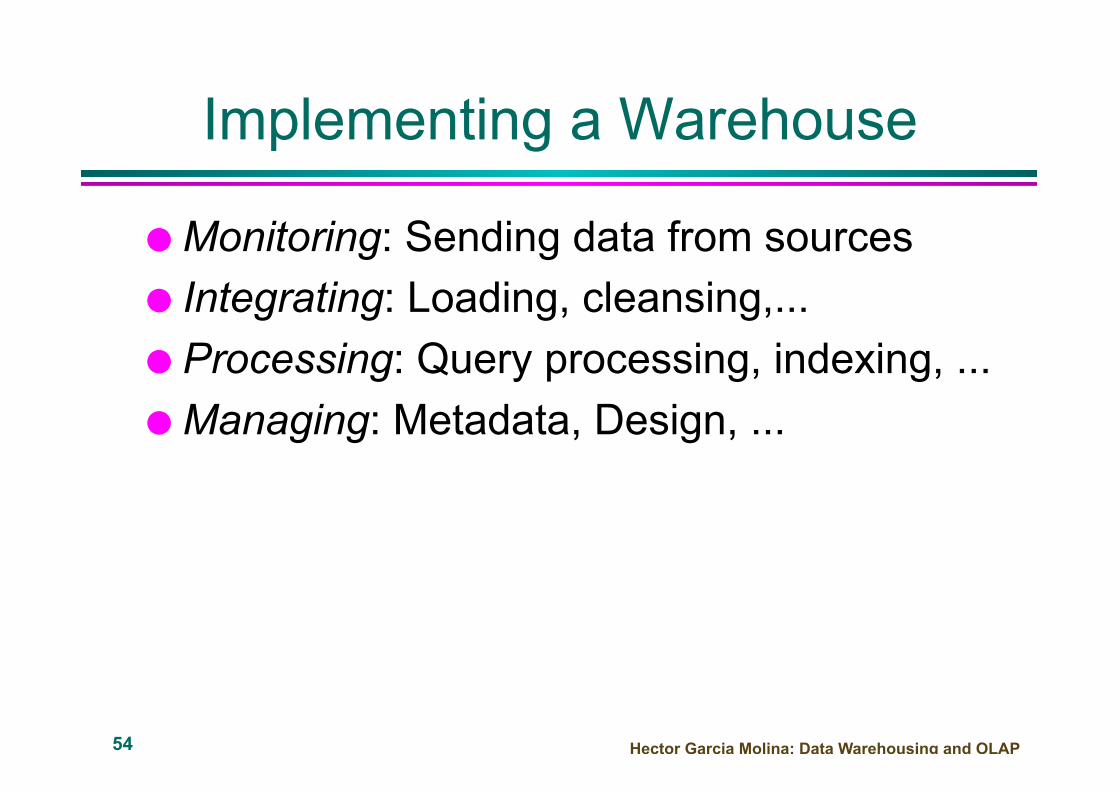
Implementing a Warehouse
Monitoring: Sending data from sources Integrating: Loading, cleansing,... Processing: Query processing, indexing, ... Managing: Metadata, Design, ...
Hector Garcia Molina: Data Warehousing and OLAP 55
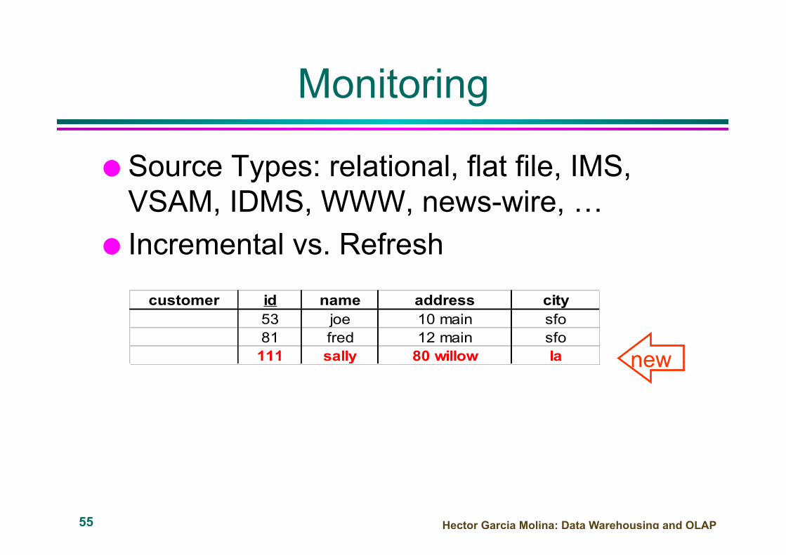
Monitoring
Source Types: relational, flat file, IMS, VSAM, IDMS, WWW, news-wire, …
Incremental vs. Refresh
customer id name address city53 joe 10 main sfo81 fred 12 main sfo
111 sally 80 willow la new

Hector Garcia Molina: Data Warehousing and OLAP 56
Monitoring Techniques
Periodic snapshots Database triggers Log shipping Data shipping (replication service) Transaction shipping Polling (queries to source) Screen scraping Application level monitoring
è
Adv
anta
ges
& D
isad
vant
ages
!!
Hector Garcia Molina: Data Warehousing and OLAP 57
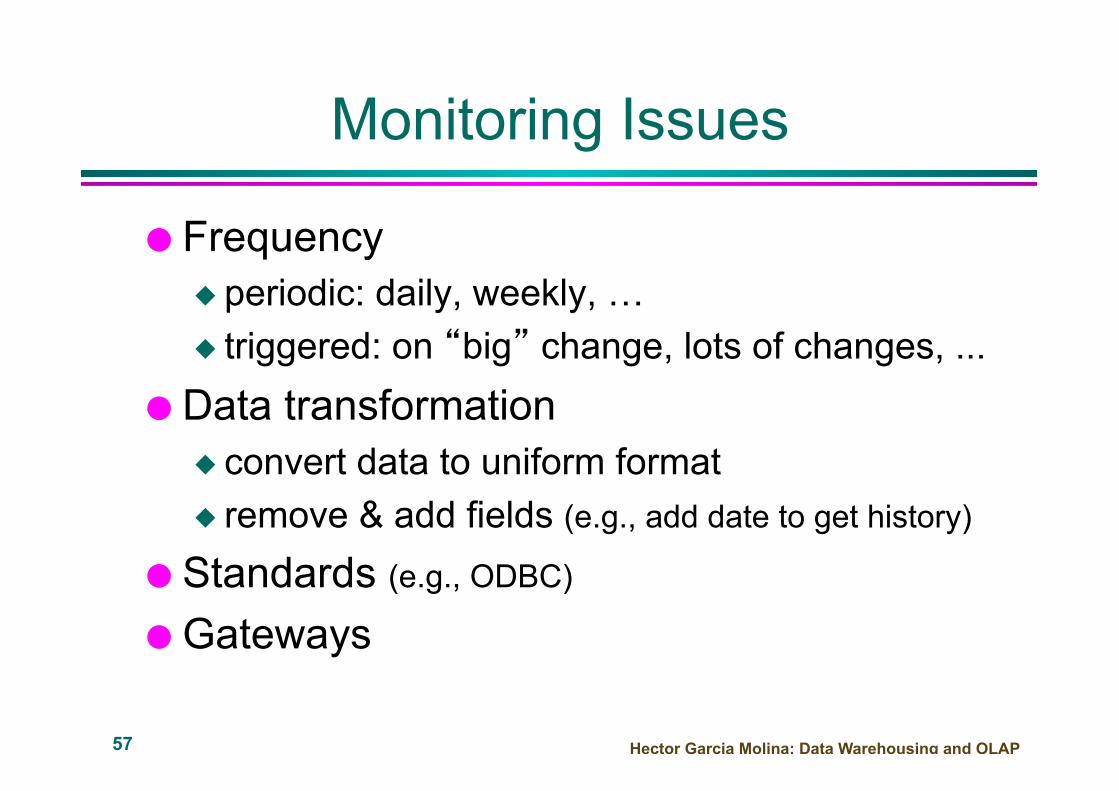
Monitoring Issues
Frequency periodic: daily, weekly, … triggered: on “big” change, lots of changes, ...
Data transformation convert data to uniform format remove & add fields (e.g., add date to get history)
Standards (e.g., ODBC) Gateways

Hector Garcia Molina: Data Warehousing and OLAP 58
Integration
Data Cleaning Data Loading Derived Data Client Client
Warehouse
Source Source Source
Query & Analysis
Integration
Metadata
Hector Garcia Molina: Data Warehousing and OLAP 59
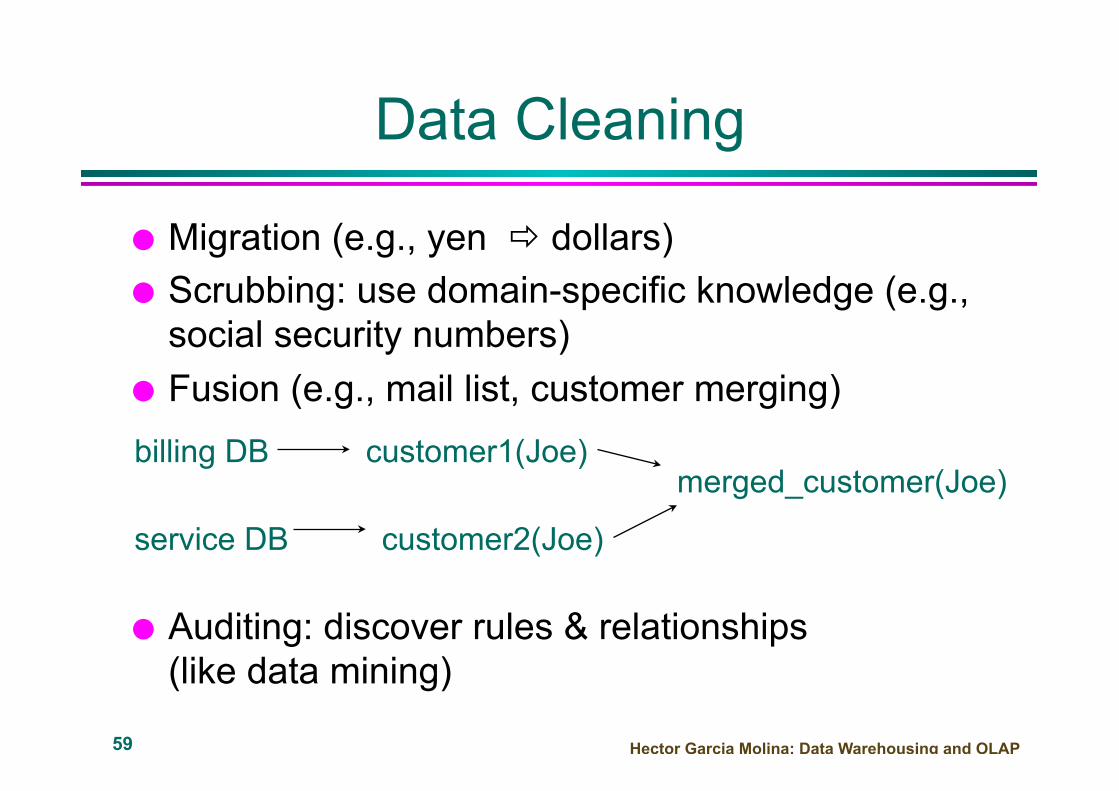
Data Cleaning
Migration (e.g., yen ð dollars) Scrubbing: use domain-specific knowledge (e.g.,
social security numbers) Fusion (e.g., mail list, customer merging) Auditing: discover rules & relationships
(like data mining)
billing DB
service DB
customer1(Joe)
customer2(Joe)
merged_customer(Joe)

Hector Garcia Molina: Data Warehousing and OLAP 60
Loading Data
Incremental vs. refresh Off-line vs. on-line Frequency of loading
At night, 1x a week/month, continuously Parallel/Partitioned load
Hector Garcia Molina: Data Warehousing and OLAP 61
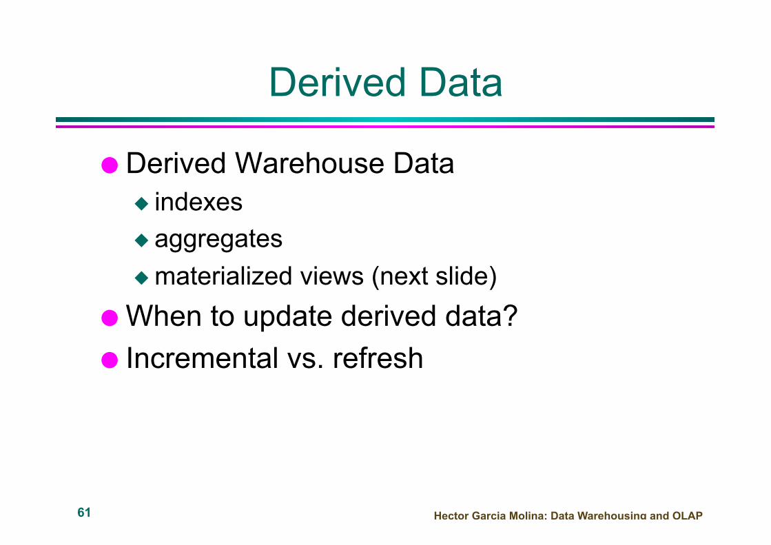
Derived Data
Derived Warehouse Data indexes aggregates materialized views (next slide)
When to update derived data? Incremental vs. refresh

Hector Garcia Molina: Data Warehousing and OLAP 62
Materialized Views Define new warehouse relations using
SQL expressions sale prodId storeId date amt
p1 c1 1 12p2 c1 1 11p1 c3 1 50p2 c2 1 8p1 c1 2 44p1 c2 2 4
product id name pricep1 bolt 10p2 nut 5
joinTb prodId name price storeId date amtp1 bolt 10 c1 1 12p2 nut 5 c1 1 11p1 bolt 10 c3 1 50p2 nut 5 c2 1 8p1 bolt 10 c1 2 44p1 bolt 10 c2 2 4
does not exist at any source
Hector Garcia Molina: Data Warehousing and OLAP 63
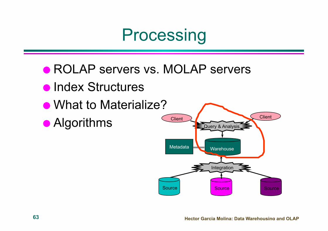
Processing
ROLAP servers vs. MOLAP servers Index Structures What to Materialize? Algorithms Client Client
Warehouse
Source Source Source
Query & Analysis
Integration
Metadata
Hector Garcia Molina: Data Warehousing and OLAP 64
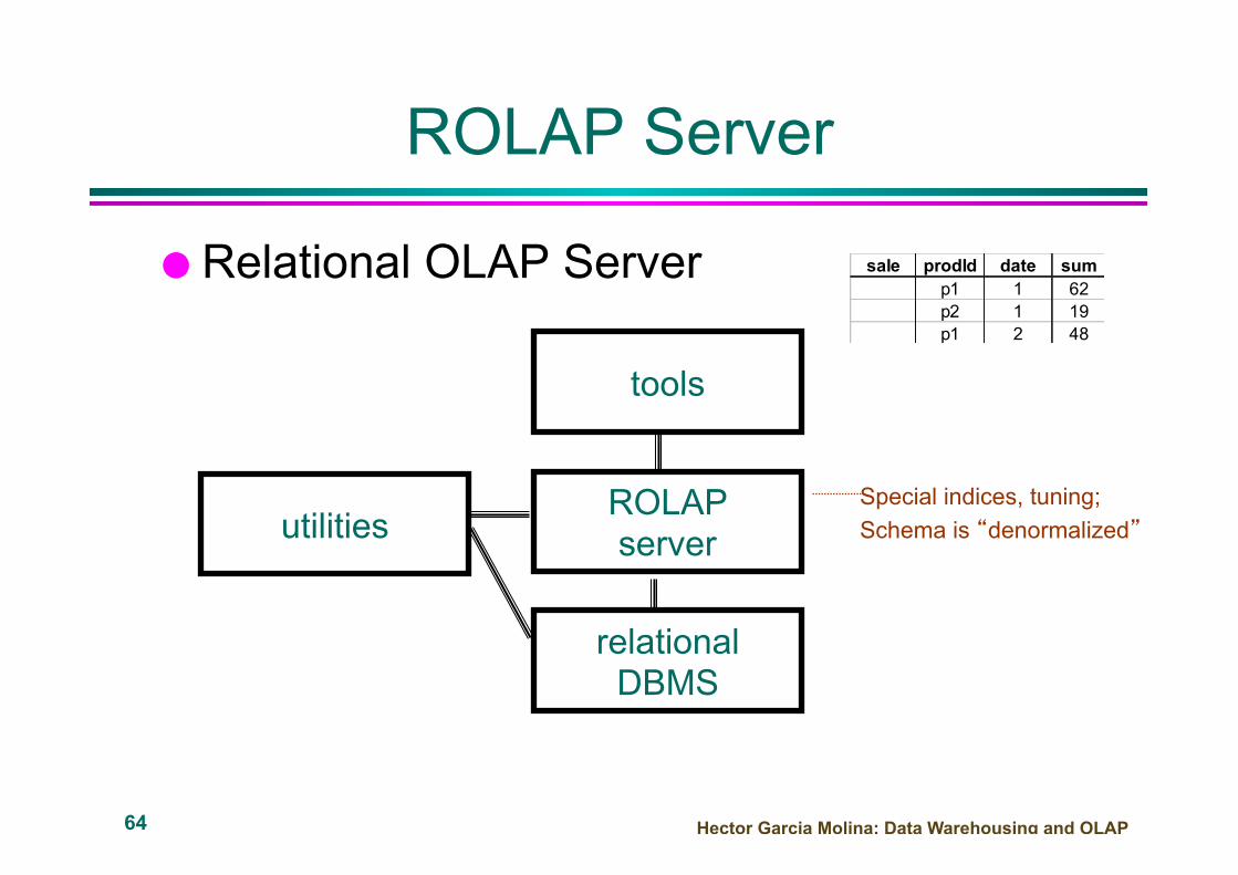
ROLAP Server
Relational OLAP Server
relational DBMS
ROLAP server
tools
utilities
sale prodId date sump1 1 62p2 1 19p1 2 48
Special indices, tuning; Schema is “denormalized”
Hector Garcia Molina: Data Warehousing and OLAP 65
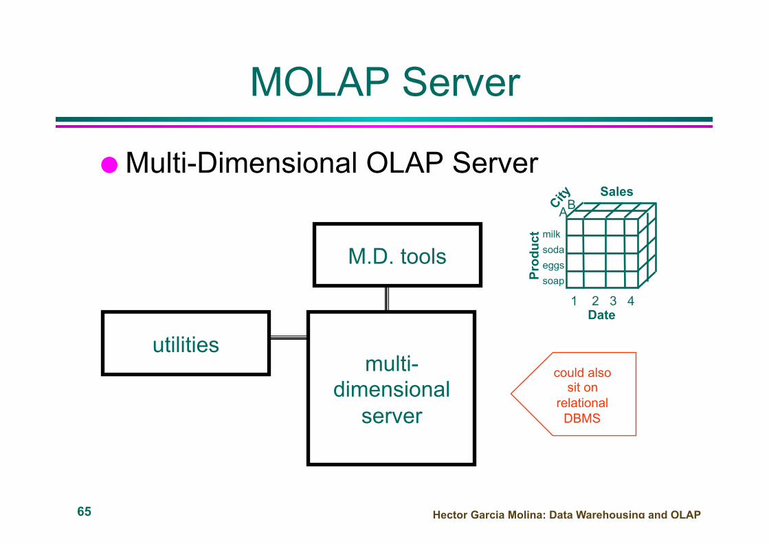
MOLAP Server
Multi-Dimensional OLAP Server
multi-dimensional
server
M.D. tools
utilities could also
sit on relational
DBMS
Prod
uct
Date 1 2 3 4
milk soda eggs soap
A B Sales

Hector Garcia Molina: Data Warehousing and OLAP 66
Index Structures
Traditional Access Methods B-trees, hash tables, R-trees, grids, …
Popular in Warehouses inverted lists bit map indexes join indexes text indexes

Hector Garcia Molina: Data Warehousing and OLAP 67
Inverted Lists
2023
1819
202122
232526
r4r18r34r35
r5r19r37r40
rId name ager4 joe 20r18 fred 20r19 sally 21r34 nancy 20r35 tom 20r36 pat 25r5 dave 21r41 jeff 26
. . .
age index
inverted lists
data records
Hector Garcia Molina: Data Warehousing and OLAP 68
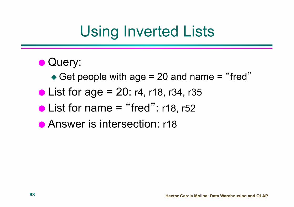
Using Inverted Lists
Query: Get people with age = 20 and name = “fred”
List for age = 20: r4, r18, r34, r35 List for name = “fred”: r18, r52 Answer is intersection: r18

Hector Garcia Molina: Data Warehousing and OLAP 69
Bit Maps
2023
1819
202122
232526
id name age1 joe 202 fred 203 sally 214 nancy 205 tom 206 pat 257 dave 218 jeff 26
. . .
age index
bit maps
data records
110110000
0010001011

Hector Garcia Molina: Data Warehousing and OLAP 70
Using Bit Maps
Query: Get people with age = 20 and name = “fred”
List for age = 20: 1101100000 List for name = “fred”: 0100000001 Answer is intersection: 010000000000
Good if domain cardinality small Bit vectors can be compressed

Hector Garcia Molina: Data Warehousing and OLAP 71
Join
sale prodId storeId date amtp1 c1 1 12p2 c1 1 11p1 c3 1 50p2 c2 1 8p1 c1 2 44p1 c2 2 4
• “Combine” SALE, PRODUCT relations • In SQL: SELECT * FROM SALE, PRODUCT
product id name pricep1 bolt 10p2 nut 5
joinTb prodId name price storeId date amtp1 bolt 10 c1 1 12p2 nut 5 c1 1 11p1 bolt 10 c3 1 50p2 nut 5 c2 1 8p1 bolt 10 c1 2 44p1 bolt 10 c2 2 4

Hector Garcia Molina: Data Warehousing and OLAP 72
Join Indexes
product id name price jIndexp1 bolt 10 r1,r3,r5,r6p2 nut 5 r2,r4
sale rId prodId storeId date amtr1 p1 c1 1 12r2 p2 c1 1 11r3 p1 c3 1 50r4 p2 c2 1 8r5 p1 c1 2 44r6 p1 c2 2 4
join index
Hector Garcia Molina: Data Warehousing and OLAP 73
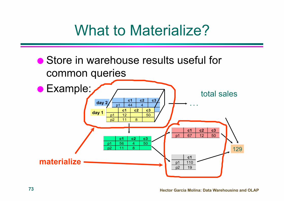
What to Materialize?
Store in warehouse results useful for common queries
Example: day 2 c1 c2 c3
p1 44 4p2 c1 c2 c3
p1 12 50p2 11 8
day 1
c1 c2 c3p1 56 4 50p2 11 8
c1 c2 c3p1 67 12 50
c1p1 110p2 19
129
. . . total sales
materialize

Hector Garcia Molina: Data Warehousing and OLAP 74
Materialization Factors
Type/frequency of queries Query response time Storage cost Update cost
Hector Garcia Molina: Data Warehousing and OLAP 75
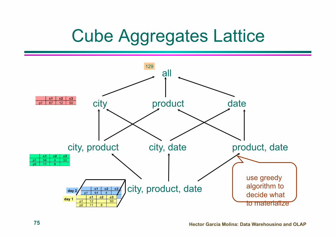
Cube Aggregates Lattice
city, product, date
city, product city, date product, date
city product date
all
day 2 c1 c2 c3p1 44 4p2 c1 c2 c3
p1 12 50p2 11 8
day 1
c1 c2 c3p1 56 4 50p2 11 8
c1 c2 c3p1 67 12 50
129
use greedy algorithm to decide what to materialize

Hector Garcia Molina: Data Warehousing and OLAP 76
Dimension Hierarchies
all
state
city
cities city statec1 CAc2 NY
Hector Garcia Molina: Data Warehousing and OLAP 77
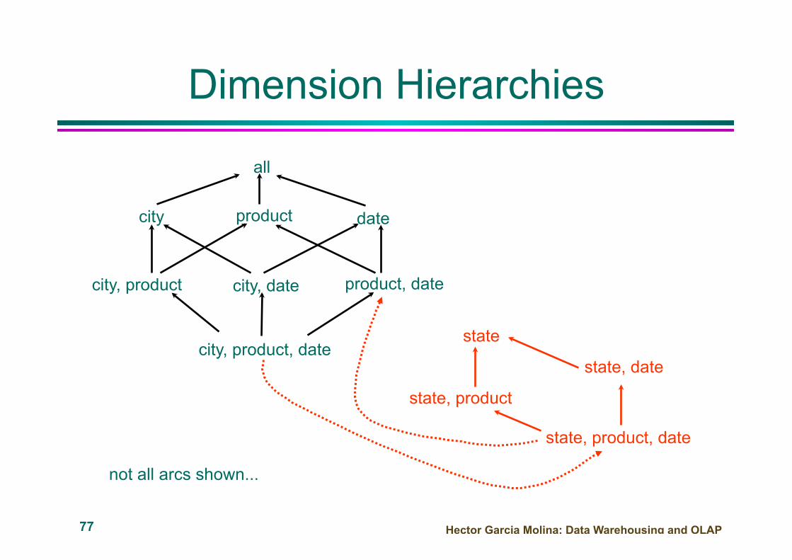
Dimension Hierarchies
city, product
city, product, date
city, date product, date
city product date
all
state, product, date
state, date state, product
state
not all arcs shown...
Hector Garcia Molina: Data Warehousing and OLAP 78
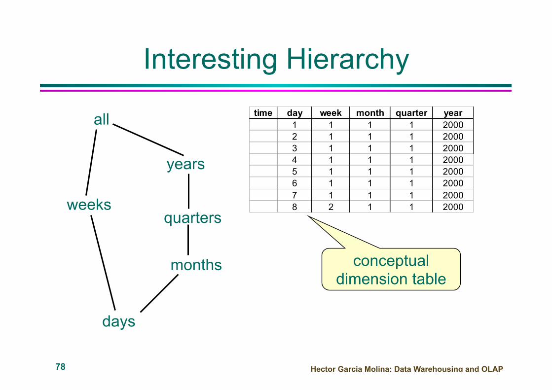
Interesting Hierarchy
all
years
quarters
months
days
weeks
time day week month quarter year1 1 1 1 20002 1 1 1 20003 1 1 1 20004 1 1 1 20005 1 1 1 20006 1 1 1 20007 1 1 1 20008 2 1 1 2000
conceptual dimension table

Hector Garcia Molina: Data Warehousing and OLAP 79
Design
What data is needed? Where does it come from? How to clean data? How to represent in warehouse (schema)? What to summarize? What to materialize? What to index?
Hector Garcia Molina: Data Warehousing and OLAP 80
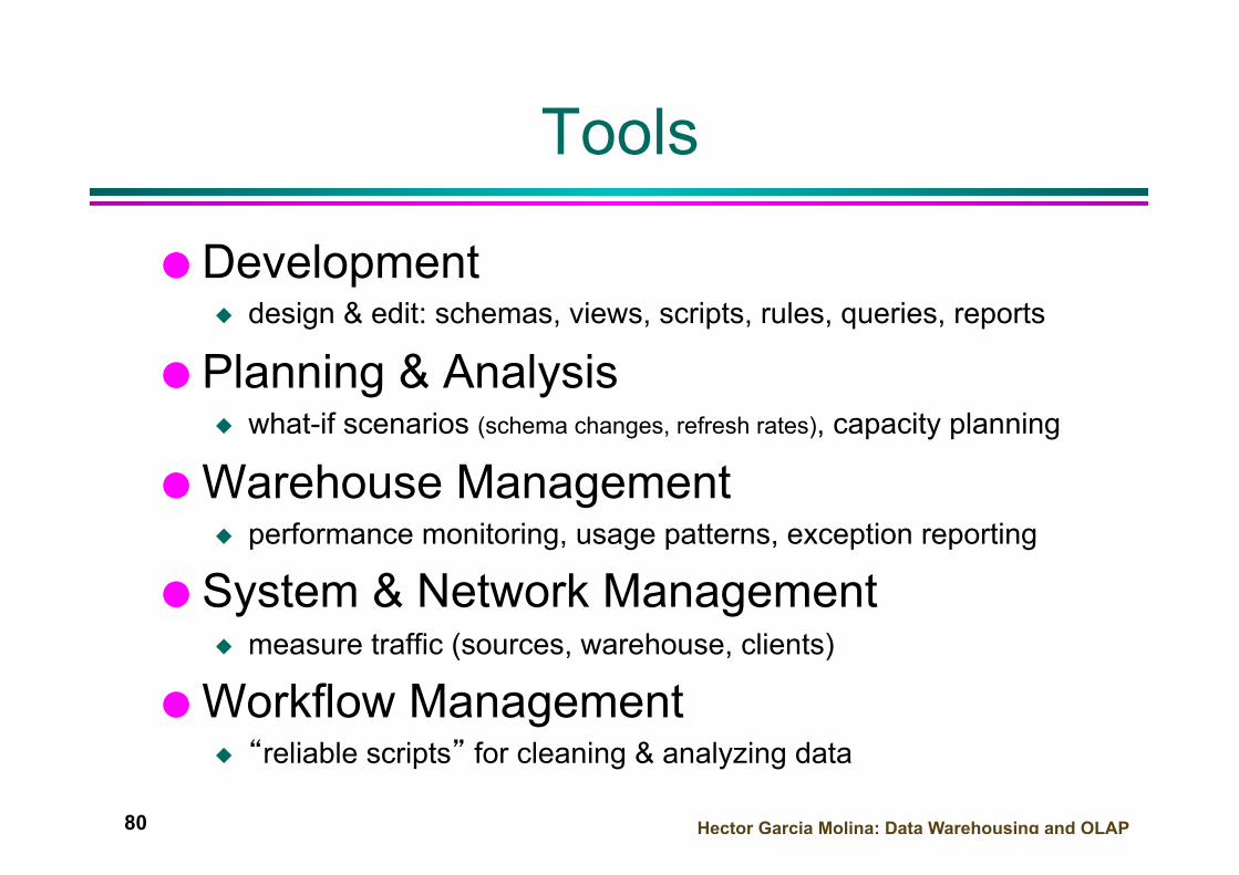
Tools
Development design & edit: schemas, views, scripts, rules, queries, reports
Planning & Analysis what-if scenarios (schema changes, refresh rates), capacity planning
Warehouse Management performance monitoring, usage patterns, exception reporting
System & Network Management measure traffic (sources, warehouse, clients)
Workflow Management “reliable scripts” for cleaning & analyzing data

DW Products and Tools
• Oracle 11g, IBM DB2, Microsoft SQL Server, ... – All provide OLAP extensions
• SAP Business Information Warehouse – ERP vendors
• MicroStrategy, Cognos (now IBM) – Specialized vendors – Kind of Web-based EXCEL
• Niche Players (e.g., Btell) – Vertical application domain
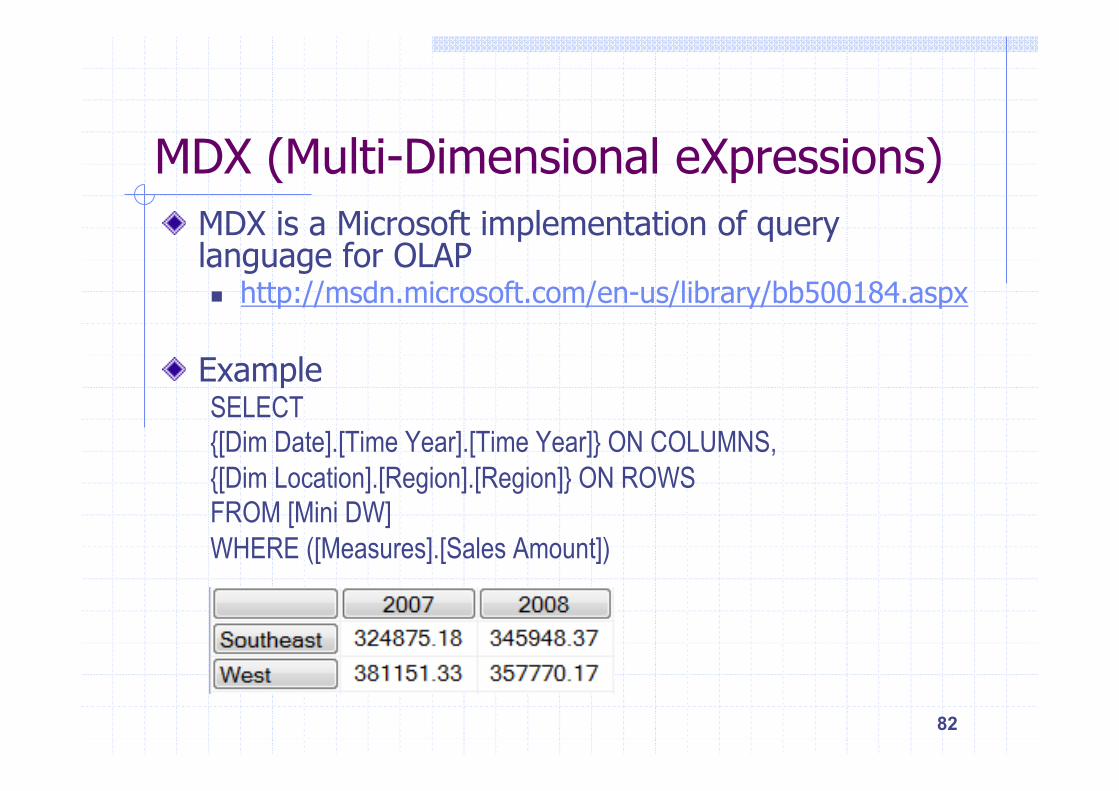
MDX (Multi-Dimensional eXpressions) " MDX is a Microsoft implementation of query
language for OLAP n http://msdn.microsoft.com/en-us/library/bb500184.aspx
" Example SELECT {[Dim Date].[Time Year].[Time Year]} ON COLUMNS, {[Dim Location].[Region].[Region]} ON ROWS FROM [Mini DW] WHERE ([Measures].[Sales Amount])
82

October 26, 2011 Data Mining: Concepts and
Techniques 83
Chapter 2: Data Preprocessing
n Why preprocess the data?
n Data cleaning
n Data integration and transformation
n Data reduction
n Discretization and concept hierarchy generation
n Summary

October 26, 2011 Data Mining: Concepts and
Techniques 84
Discretization
n Three types of attributes:
n Nominal — values from an unordered set, e.g., color, profession
n Ordinal — values from an ordered set, e.g., military or academic
rank
n Continuous — real numbers, e.g., integer or real numbers
n Discretization:
n Divide the range of a continuous attribute into intervals
n Some classification algorithms only accept categorical attributes.
n Reduce data size by discretization
n Prepare for further analysis

October 26, 2011 Data Mining: Concepts and
Techniques 85
Discretization and Concept Hierarchy
n Discretization
n Reduce the number of values for a given continuous attribute by
dividing the range of the attribute into intervals
n Interval labels can then be used to replace actual data values
n Supervised vs. unsupervised
n Split (top-down) vs. merge (bottom-up)
n Discretization can be performed recursively on an attribute
n Concept hierarchy formation
n Recursively reduce the data by collecting and replacing low level
concepts (such as numeric values for age) by higher level concepts
(such as young, middle-aged, or senior)

October 26, 2011 Data Mining: Concepts and
Techniques 86
Segmentation by Natural Partitioning
n A simply 3-4-5 rule can be used to segment numeric data
into relatively uniform, “natural” intervals.
n If an interval covers 3, 6, 7 or 9 distinct values at the
most significant digit, partition the range into 3 equi-
width intervals
n If it covers 2, 4, or 8 distinct values at the most
significant digit, partition the range into 4 intervals
n If it covers 1, 5, or 10 distinct values at the most
significant digit, partition the range into 5 intervals

October 26, 2011 Data Mining: Concepts and
Techniques 87
Example of 3-4-5 Rule
(-$400 -$5,000)
(-$400 - 0) (-$400 - -$300) (-$300 - -$200) (-$200 - -$100)
(-$100 - 0)
(0 - $1,000) (0 - $200) ($200 - $400)
($400 - $600)
($600 - $800) ($800 -
$1,000)
($2,000 - $5, 000)
($2,000 - $3,000)
($3,000 - $4,000)
($4,000 - $5,000)
($1,000 - $2, 000) ($1,000 - $1,200)
($1,200 - $1,400)
($1,400 - $1,600)
($1,600 - $1,800) ($1,800 -
$2,000)
msd=1,000 Low=-$1,000 High=$2,000 Step 2:
Step 4:
Step 1: -$351 -$159 profit $1,838 $4,700 Min Low (i.e, 5%-tile) High(i.e, 95%-0 tile) Max
count
(-$1,000 - $2,000)
(-$1,000 - 0) (0 -$ 1,000) Step 3:
($1,000 - $2,000)
Example
October 26, 2011 Data Mining: Concepts and Techniques 88
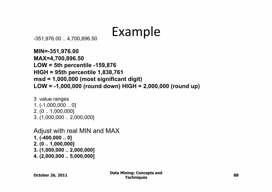
-351,976.00 .. 4,700,896.50 MIN=-351,976.00 MAX=4,700,896.50 LOW = 5th percentile -159,876 HIGH = 95th percentile 1,838,761 msd = 1,000,000 (most significant digit) LOW = -1,000,000 (round down) HIGH = 2,000,000 (round up) 3 value ranges 1. (-1,000,000 .. 0] 2. (0 .. 1,000,000] 3. (1,000,000 .. 2,000,000] Adjust with real MIN and MAX 1. (-400,000 .. 0] 2. (0 .. 1,000,000] 3. (1,000,000 .. 2,000,000] 4. (2,000,000 .. 5,000,000]
Jaak Vilo and other authors UT: Data Mining 2009 89
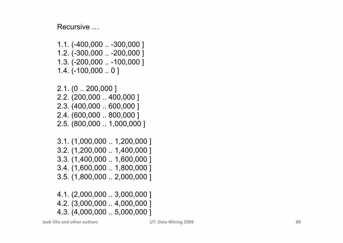
Recursive … 1.1. (-400,000 .. -300,000 ] 1.2. (-300,000 .. -200,000 ] 1.3. (-200,000 .. -100,000 ] 1.4. (-100,000 .. 0 ] 2.1. (0 .. 200,000 ] 2.2. (200,000 .. 400,000 ] 2.3. (400,000 .. 600,000 ] 2.4. (600,000 .. 800,000 ] 2.5. (800,000 .. 1,000,000 ] 3.1. (1,000,000 .. 1,200,000 ] 3.2. (1,200,000 .. 1,400,000 ] 3.3. (1,400,000 .. 1,600,000 ] 3.4. (1,600,000 .. 1,800,000 ] 3.5. (1,800,000 .. 2,000,000 ] 4.1. (2,000,000 .. 3,000,000 ] 4.2. (3,000,000 .. 4,000,000 ] 4.3. (4,000,000 .. 5,000,000 ]

Concept Hierarchy Generation for Categorical Data
• Specification of a partial/total ordering of attributes explicitly at the schema level by users or experts
– street < city < state < country
• Specification of a hierarchy for a set of values by explicit data grouping
– {Urbana, Champaign, Chicago} < Illinois
• Specification of only a partial set of attributes
– E.g., only street < city, not others
• Automatic generation of hierarchies (or attribute levels) by the analysis of the number of distinct values
– E.g., for a set of attributes: {street, city, state, country} October 26, 2011 Data Mining: Concepts and Techniques 90
October 26, 2011 Data Mining: Concepts and
Techniques 91
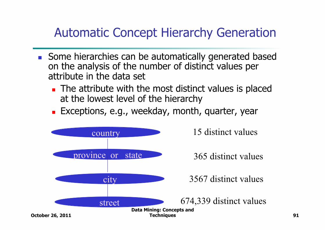
Automatic Concept Hierarchy Generation
n Some hierarchies can be automatically generated based on the analysis of the number of distinct values per attribute in the data set n The attribute with the most distinct values is placed
at the lowest level of the hierarchy n Exceptions, e.g., weekday, month, quarter, year
country
province_or_ state
city
street
15 distinct values
365 distinct values
3567 distinct values
674,339 distinct values
Summary
• OLAP and DW – a way to summarise data
• Prepare data for further data mining and visualisaKon
• Fact table, aggregaKon, queries&indeces, …
• Jaak Vilo and other authors UT: Data Mining 2009 92
93
Reference (highly recommended)
• Jim Gray et al. “Data Cube: A Relational Aggregation Operator Generalizing Group-By, Cross-Tab, and Sub-Totals”. Data Mining and Knowledge Discovery 1(1), 1997.
• http://citeseer.ist.psu.edu/old/392672.html • Data Warehousing chapter of Jianwei Han’s
textbook (chapter 3)
94
Homework
• Exercises 1 and 4 at: – http://www.systems.ethz.ch/education/courses/fs09/
data-warehousing/ex2.pdf • Multidimensional data modeling exercise in
course Wiki pages