Data Type : The data type can be specified by selecting a particular column and choosing the Data validation.

Data constraint: It is a way to control the user’s mistake. Through which user can be guided about the insertion of wrong data.

It has Three parts –

• Data Validation - It checks whether the data meets the constraint or not.• Warning/Error Alert - This helps people to warn about any wrong entry.• Input Message – This guides the user to enter the data .

Sorting

It can be defined as a processing technique to –

• Arrange systematically in groups; separate according to type, class, etc.

• Look at (a group of things) one after another in order to classify them or make a selection.

Why is it necessary?

It is necessary to• Obtain the required uniformity•Ensure to get only the desired of data from huge database.

Types:

It may be

• Ascending or Descending - ( a to z or z to a . For text and 0 to 10 or 10 to 0 for number)

• Multiple or Single - May be on single field or may be on more than one field.

• Row or Column wise

• Case Sensitive or not

• Random sorting

• Custom Sorting- to sort data into a recognizable order that is not alphabetical. For example, regions listed as “East", "Central" and then "West". Using a regular sort, there is not a good way to force E to sort before C and W.

To do that ,-

1.Click the Sort option in the Sort & Filter group. (Don’t click the A to Z or Z to A sort icons, the ones with the arrows.)

2. In the resulting Sort dialog box, click the Order control’s dropdown list and choose the appropriate custom sort.

3.Click OK. When using a custom sort, the list doesn’t have to contain all of the sort elements to work. A list of just a few months will still sort by month order when applying the custom sort.

• Random Sorting-

•Next to list, add a heading called Random .•Select all of the cells next to this column of names. Type =RAND()

• Hit Ctrl+Enter to enter the cells in all of the cells in the selection.

• Sort by column B to get a random sequence.

Filtering

Definition : It is a technical process to pass through a device or tool to remove unwanted material / data. It is a program that is designed to examine each input or output request for certain qualifying criteria and then process it accordingly.

Filtered data displays only the rows that meet criteria and hides rows that do not want to display . After filtering data, one can copy, find, edit, format, chart, and print the subset of filtered data without rearranging or moving it.

Types : It is two types – 1) Autofilter- can be subdivided as

• by a list values• by a format• by criteria

2) Advanced FilterEach of these filter types is mutually exclusive for each range of cells or column table.

Filter text

Range of cells    Select a range of cells containing alphanumeric data.

Setting criteria   

1. to filter by text that begins with a specific character(select Begins With), or to filter by text that has specific characters anywhere in the text, select Contains.

2. In the Custom AutoFilter dialog box, enter text or select the text value from the list.

Example, to filter by text that begins with the letter "J", enter J, or to filter by text that has "bell" anywhere in the text, enter bell.

3. to find text that shares some characters but not others, use a wildcard character. How to use wildcard charactersThe following wildcard characters can be used as comparison criteria for text filters.

Use To find

? (question mark)Any single characterFor example, sm?th finds "smith" and "smyth"

* (asterisk)Any number of charactersFor example, *east finds "Northeast" and "Southeast"

~ (tilde) followed by ?, *, or ~ A question mark, asterisk, or tildeFor example, fy06~? finds "fy06?"

Filter Numbers

Range of cells    Select a range of cells containing numeric data. Select from a list of numbers

Set criteria1. Point to Number Filters and then click Custom Filter. Example, to filter by a lower and upper number limit, select Between.2. In the Custom AutoFilter dialog box, enter numbers or select numbers from the list. Example, to filter by a lower number of 25 and an upper number of 50, enter 25 and 50.

Filter dates or times

Select from a list of dates or times.  

By default, all dates in the range of cells are grouped by a hierarchy of years, months, and days. Selecting a higher level in the hierarchy selects all nested dates below that level. .

Example, if you select 2006, months are listed below 2006, and days are listed below each month

Setting criteria    Point to Date Filters and then do one of the following: i) Common filter    - is one based on a comparison operator.Select any comparison operator commands (Equals, Before, After, or Between ) or click Custom Filter.In the Custom AutoFilter dialog box, enter/select a date or time, select a date or time from the list, or click the Calendar button to find and enter a date.

Example, to filter by a lower and upper date or time, select Between.

For example, to filter by an earlier date of "3/1/2006" and a later date of "6/1/2006", enter 3/1/2006 and 6/1/2006. Or, to filter by an earlier time of "8:00 AM" and a later time of "12:00 PM", enter 8:00 AM and 12:00 PM.

ii) Dynamic filter    - is one where the criteria can change when you reapply the filter.

Example, to filter all dates by the current date, select Today, or by the following month, select Next Month - Click OK.

The commands , the All Dates in the Period menu, such as January or Quarter 2, filter by the period no matter what the year. This can be useful, to compare sales by a period across several years.

This Year and Year to Date are different in the way that- This Year can return dates in the future for the current year, whereas Year to Date only returns dates up to and including the current date.

Other types of Filter

Filter for top or bottom numbers Filter for average or below average number Filter for blank or no blank Filter by cell color, font color - click Filter by Selected Cell's Color/Filter by Selected Cell's Font Color Filter by Selected Cell's Value / or by selection.

ADVANCED FILTER

It is a complex filtering process. We can set a single or more than one criteria at a time using ‘AND’ and ‘OR’ options and different operators like >,< = , <> etc.To perform advanced filter, following steps are –

1. Set up the Criteria Range (optional)In the criteria range for an Excel advanced filter, you can set the rules for the data that should remain visible after the filter is applied. You can use one criterion, or several.

• Example, cells F1:F2 are the criteria range.• The heading in F1 exactly matches a heading (D1) in the database and cell F2 contains the criterion. • The > (greater than) operator is used, with the number

500 (no $ sign is included).After the Excel advanced filter is applied, orders with a total greater than $500 will remain visible.

Other operators include:< less than <= less than or equal to >= greater than or equal to <> not equal to Apply the Excel Advanced Filter Select a cell in the database.On the Excel Ribbon's Data tab, click the Advanced Filter dialog box.

• You can choose to filter the list in place, or copy the results to another location.• You can select the cells on the worksheet or the list range is automatically detected.• Select the criteria range on the worksheet.• If you are copying to a new location, select a starting cell for the copy• Click OK

• If you copy to another location, all cells below the extract range will be cleared when the Advanced Filter is applied.

Filter Unique RecordsYou can extract a list of unique items in the database. For example, get a list of customers from an order list, or compile a list of products sold. The unique list can be copied to a different location, and the original list remains unchanged.

Note: The list must contain a heading, other wise, the first item may be duplicated in the results. To copy the data to another location –• Select a cell in the database, in the Advanced Filter dialog box,choose 'Copy to another location'.• For the List range, select the column(s) from which you want to extract the unique values.• Leave the Criteria Range blank.

Setting up the Criteria Range

•Select a starting cell for the Copy to location .Add a check mark to the Unique records only box. Then Click OK.

AND vs OR

AND – Is used when more than one criteria should be satisfied at a time. Ex.

OR – is used when mutually exclusive criteria are applied .

• the customer must be MegaMart • AND the product must be Cookies • AND the total must be greater than 500.

• the customer must be MegaMart • OR the product must be Cookies • OR the total must be greater than 500.

Combination of the AND and OR operators. • the customer must be MegaMart AND the product must be Cookies

OR • the product must be Cookies AND the total must be greater than 500.

Using Wildcards in CriteriaUse wildcard characters to filter for a text string in a cell. The * wildcard The asterisk (*) wildcard character represents any number of characters in that position, including zero characters.

The ? wildcard The question mark (?) wildcard character represents one(single) characters in that particular position.

The ~ wildcard The tilde (~) wildcard character lets you search for characters that are used as wildcards.

Extract Items with Specific TextWhen we use text as criteria Excel finds all items that begin with that text.

Extract Items in a RangeTo extract a list of items in a range, we can use two columns for one of the fields.

Create Two or More Sets of ConditionsIf you enter criteria on different rows in the criteria range, you create an OR statement.

1. Sort the Data with Score in Descending Order.

2. Sort the Data with Dept in Asc. order and Score in Des.order.

6. Filter the data only for the Grade A candidates and copy it to a different location with new data range name .

3. Go to the original database and sort those randomly to get a random sequence against the name of the employees.

Tutorial on Sort and FilterOpen the employee database and perform the following

4. Clear the sort. Find department wise frequency distribution of ave. score with a suitable chart title and legend.

5. Create a new list using custom list and sort grade according to the new list.

9. Filter those records who are the employees of MRKT and name started with “AB”. Copy at different location.10. Perform the same with name started as ’ach’.11. Filter only those records whose score greater than 9.0 and less than 13.0.12. Filter only the name ‘ANKITA’ using wild card character. 13. Filter those records whose score =>9.0 and who is an employee of dept. ‘PROD’.14. Display the list of female employees who belongs to HR Dept.15. Display all female employees who get the score>=10.0.16. Display only unique records and paste it to a different location.

7. Clear filter of the original data and filter only those records - whose name starts with ‘ABH’ - Whose name that contains ‘Agarwal

8. Display only MKT’s employees record.

VLOOKUP AND HLOOKUP

Definition: It is a tool or process technique that helps us to find out a particular item vertically or Horizontally i.e looking values down in a column or from left to right in a row.

USE: The VLOOKUP and HLOOKUP functions contain an argument called range_lookup that allows you to find an exact match to your lookup value without sorting the lookup table. Create a Lookup Table A B C D

1 Code Product Price

2 A23 Paper 5.00

3 B14 Lamp 15.00

4 A27 Desk 75.00

5 C45 Pencil 0.50

6      

1. Enter the headings in the first row

2. The first column should contain the unique key values on which you will base the lookup.

Example, you can find the price for a specific product code.

3. If you have other data on the worksheet, leave at least one blank row at the bottom of the table, and one

blank column at the right of the table, to separate the lookup table from the other data.

Excel VLOOKUP Function ArgumentsThe Excel VLOOKUP function has four arguments:

1. lookup_value:The value that I want to look up or find.

2. table_array: If you use an absolute reference like ($A$2:$C$5), instead of a relative reference like (A2:C5), it will be easier to copy to formula to other cells. Or, name the lookup table, and refer to it by name.

3. col_index_num: The column number that has the value you want returned. In this example, the product names are in the second column of the lookup table.

4.[range_lookup]: It specifies whether you want an exact match or an approximate match.

If you use TRUE as the last argument, or omit the last argument, then an approximate match can be returned. When the FALSE is used as the last argument, so if the product code is not found, the result will be #N/A.

Note: It will accept 0 instead of FALSE, and 1 instead of TRUE     .

http://www.contextures.com/xlfunctions02.html

HLOOKUP

=HLOOKUP(lookup_value,table_array,row_index_num,range_lookup)

Argument Definition of argument

lookup_value The value to be found in the first row of the array.

table_array The table of information in which data is looked up.

row_index The row number in the table_array for which the matching value should be returned.

range_lookup It is a logical value that specifies whether you want to find an exact match or an approximate match. If

TRUE or omitted, an approximate match is returned; in other words, if an exact match is not found, the next largest value that is less than the lookup_value is returned. If FALSE, HLOOKUP finds an exact match. If an exact match is not found, the #N/A error value is returned.

If range_lookup is TRUE or omitted (for an approximate match), the values in the first row of table_array must be sorted in ascending order. If range_lookup is FALSE (for an exact match), the table_array does not need to be sorted.

Tutorial for Vlookup and Hlookup

Open the vlookup data excel file and perform the following.1. Find out the revenue for each product in sheet2 from sheet1

using vlookup function.

2. Calculate the profit for each product in sheet2.

3. Find out the approximate profit for product–O using vlookup function.

4. Transpose the data of sheet2 in sheet3 and find out the cost and approximate profit of product-G using Hlookup function.

5. Find the date of joining and department of the employee ‘MONIKA RATHORE ‘ from empdatabase using vlookup function.

6. Check the result for following (use transposed data of sheet3): - Hlookup(“product-K”, table_array,2,false)

- Hlookup (“product-K”,table_array,3,false) - Hlookup(“product-Q”,table_array,2,true) - Hlookup(“product-Q”,table_array,2,false)

GOAL SEEKDefinition: It is a process of finding the correct input when only the output is known.

In other words, the process of calculating an output by performing various what-if analysis on a given set of inputs. This function is built into certain software programs such as Microsoft Excel and can be access by typing in a specific operator in the formula.

USE : • Allows to alter the data used in a formula in order to find

out what the results will be.

• The different results can then be compared to find out which one best suits your requirements.

• Use for forecasting STEPS: 1. Create a worksheet that contains a formula, an empty variable cell that will hold your solution, and any data you need to use in your calculation.

2. The variable cell must be blank. The formula cell determines the value in the variable cell.

3. Select the cell containing the formula.

4. On the Tools menu, click Goal Seek. The Goal Seek dialog box opens to supply three variables, "Set cell1 ,to value, by changing cell2.“

5. Enter cell reference and corresponding values. Press OK.

Excel will display the Goal Seek Status dialog box when the iteration is complete, and the result for forecasting will appear in the worksheet

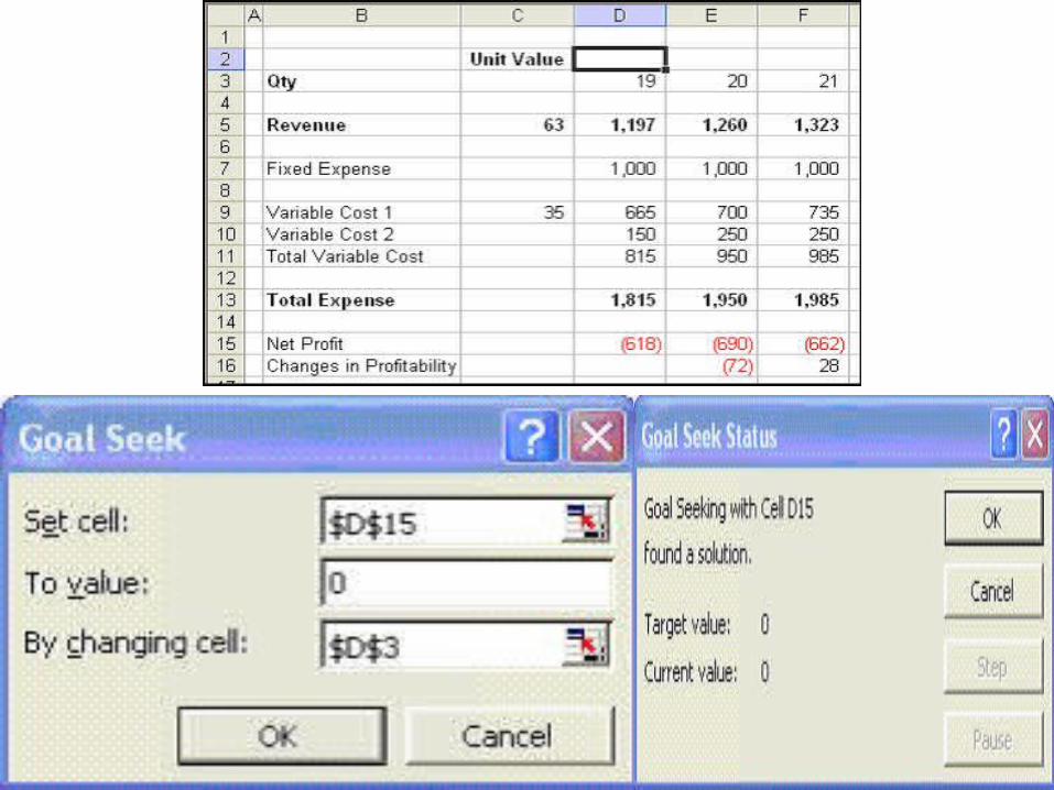
Breakeven Analysis using Goal Seek

Definition:- It is a point where the total expenses equals the total revenues. It can also be defined as the point where the net profit is zero, i.e. the company has neither made any profits nor incurred any loss.

Calculation of the Breakeven Point :-

Break even point = fixed cost / contribution margin per unit Contribution (per unit) = selling price (per unit) - variable cost (per unit)

The variables required for break even point analysis are –

• Total Variable Cost:The product of unit sales and variable unit cost.(Unit Sales * Variable Unit Cost )

• Unit Price:The amount of money charged to the customer for each unit of a product or service. • Unit Sales:Number of units of the product projected to be sold over a specific period of time. • Variable Unit Cost:Costs that vary directly with the sales and production of one additional unit. Example, commission on sales. • Fixed Cost:The sum of all costs required to produce the first unit of a product. Example, administration costs.

•Total Cost:The sum of the fixed cost and total variable cost for any given level of production and sales. (Fixed Cost + Total Variable Cost ) • Total Revenue:The product of expected unit sales and unit price. (Unit Sales * Unit Price ) • Net Profit (or Loss):(Total Revenue - Total Costs)

Therefore, Break even analysis depends on the following variables

• The fixed production costs for a product. • The variable production and sales costs for a product. • The product's unit price. • The product's expected unit sales.

Limitations• As it depends on the different costs, it is not a fixed point and its value varies with adjusting different costs - both fixed and variable - and identify areas where you might be able to make cuts.

• Breakeven analysis is not a predictor of demand, so if a market with the wrong product or the wrong price, it may be tough to ever hit the breakeven point.

Calculate Profit Breakeven Using Goal Seek

Consider the example - Fill in the boxes as shown below:

Set Cell is reference to the net profit cell D15.To Value is to instruct Goal Seek to set the net profit to zero by changing the value in certain cell, which in our example is the quantity.

Benefits / Advantages of Break Even Analysis:

The main advantages of break even point analysis are -

• It explains the relationship between cost, production, volume and returns.

• It can be extended to show how changes in fixed cost, variable cost, commodity prices, revenues will effect profit levels and break even points.

• Break even analysis is most useful when used with partial budgeting, capital budgeting techniques.

• The major benefits to use break even analysis is that it indicates the lowest amount of business activity necessary to prevent losses.

ScenarioDefinition: -

It is a specific set of values that Excel can save and automatically substitute into Worksheet. A spreadsheet displaying numerical data that is relevant to a certain date, month, topic or whatever and using the Scenario Manager we can enter different values into the worksheet to forecast the outcome of the data. These values (or Scenarios) can be retained for future use and are stored in a hidden part of the workbook which can be retrieved by asking the Scenario Manager to show the Scenario that uses those specific values.

Scenario Manager is a tool that can be used to determine different projected outcomes of data by changing different cells within a Worksheet model.

Steps:- First set up a base or default Scenario , from which all other Scenarios are defined.

• Go to Tools>Scenarios to activate the Scenario Manager. A message "No Scenarios are defined“ is displayed.• Choose Add to add the default Scenario with a name through which you can indentify . • Select the box Changing cells: The active cell in the workbook will be referenced here.

• There are two options at the bottom of this dialog box. - Prevent changes – helps to lock the scenario and will be unable to be edited. - Hide –helps to hide the Scenarios.

• Click the OK button.

•The Scenario Values dialog box will appear to enter values into the scenario cells. As the first scenario is the default Scenario, the values in the cells that we specified in the Changing Cells: box have been picked up values automatically and save with a name.

1

2

3

4

2

Adding ScenariosBy adding a new scenario new and adjust the changing values.

1

2

Displaying ScenariosBy asking the Scenario Manager to show a particular scenario. Select Tools>ScenariosClick on the Scenario name you want to see then Show.

Create a Report from a ScenarioFrom the Scenario Manager dialogue box, click the Summary button to see the following dialogue box:

A Click OKScenario summary will be displayed.

Tutorial for Goal Seek and ScenarioOpen data base sales data and perform the following.1. Forecast the unit of items to be sold to make a profit 75000 per

month by keeping the same selling price using goal seek.

2. Open the breakeven database and perform the following. - Find out the changing profitability by changing the selling

quantity (1 unit). - Find out the profit and no. of items to be sold at break even point.

3. Open the family budget database and perform the following.- calculate the profit and save the original values and save

this scenario with a name “ original budget’- Create new scenario with “suggested Budget” to make a

higher profit by changing the values of food , phone bills and clothes.

4. Open the summary repot to analyze and compare the original and suggested budget.

5. Insert a pivot table.

PIVOT TABLE

Definition:- A pivot table is a user created summary table of original spreadsheet. We can create the table by defining which fields to view and how the information should be displayed. Based on our field selections, Excel organizes the data so we see a different view of our data. A Pivot Table is way to present information in a report format. Use: • A pivot table can aggregate your information .• Showing a new perspective by moving columns to rows

or vice versa.

Pivot Table StructuresThe main areas of the pivot table.

(1) PivotTable Field List – this section in the top right displays the fields in our spreadsheet. We may check a field or drag it to a quadrant in the lower portion.

(2) The lower right quadrants - This area defines where and how the data shows on our pivot table. We can have a field show in either a column or row. We may also indicate if the information should be counted, summed, averaged, filtered and so on.

(3) The red outlined area to the left is the result of our selections from (1) and (2).

Steps to Create an Excel Pivot Table

1. Open original spreadsheet and remove any blank rows or columns.2. Make sure each column has a heading, as it will be carried over to the Field List.3. Make sure cells are properly formatted for their data type.4. Highlight data range5. Click the Insert tab.6. Select the PivotTable button from the Tables group.7. Select PivotTable from the list.

The Create PivotTable dialog appears.8. Check Table/Range: value.9. Select the radio button for New Worksheet.10. Click OK.A new worksheet opens with a blank pivot table. The fields from source spreadsheet were carried over to the PivotTable Field List.

11. Drag an item such as PRECINCT from the PivotTable Field List down to the Row Labels quadrant. The left side of Excel spreadsheet should show a row for each precinct(area/zone) value. A checkmark appears next to PRECINCT.

12. The next step is to ask what would like to know about each precinct. Such as PARTY field from the PivotTable Field List to the Column Labels quadrant. This will provide an additional column for each party.

13. To see the count for each party, need to drag the same field to the Values quadrant. By double-clicking the entry and another Field Setting can be chosen. Excel has also added Grand Totals.

Additional Groupings and OptionsA sub grouping under a group is also provided by pivot table .For example, we might want to know the Age Range of voters by Precinct by Party. In this case, we would drag the AGE GROUP column from the PivotTable Field List down below the PRECINCT value in Row Labels.

Pivot table defers form normal spreadsheet

One area that is different is the pivot table has its own options.

• By right-clicking a cell within and selecting PivotTable Options… For example, we might only want Grand Totals for columns and not rows.

• There are also ways to filter the data using the controls next to Row Labels or Column labels on the pivot table. We may also drag fields to the Report Filter quadrant.

TUTORIAL FOR PIVOT TABLE

Open Sales data and perform the following.-

1. Show the region wise selling pattern for all sales persons and their total sales amount.

2. Display the product wise sales for each region.

3. Compare the monthly selling performance for each sales person.

4. Draw a pivot chart showing monthly regional selling status. Change the chart according to product sales.

5. Open the student data. Display the month wise sum of score for all subjects and their grand total.

6. Display the highest score for each students.

7. Display the pivot chart for student’s monthly score.