Data StructuresAdvanced Sorts Part 2:

QuicksortPhil Tayco

Slide version 1.0

Mar. 22, 2015

Advanced Sorts

Divide and Conquer

• The mergesort algorithm shows that using the divide and conquer approach can lead to improving the sort algorithms from O(n2) to O(n log n)

• Its challenge is that it requires twice the memory space of the size of the array we are trying to sort

• To combat this, we need to combine a divide and conquer approach with an idea that allows us to not require a temp array

• Without a temp array, we’ll need to figure out how improve the sort process using swaps and/or shifts

Advanced Sorts

Mergesort as a model

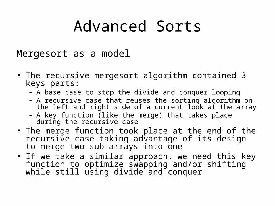
• The recursive mergesort algorithm contained 3 keys parts:– A base case to stop the divide and conquer looping– A recursive case that reuses the sorting algorithm on the

left and right side of a current look at the array– A key function (like the merge) that takes place during the

recursive case• The merge function took place at the end of the

recursive case taking advantage of its design to merge two sub arrays into one

• If we take a similar approach, we need this key function to optimize swapping and/or shifting while still using divide and conquer

Advanced Sorts

Left and right

• To use divide and conquer effectively, we need to look at ways to cleverly and recursively split the array

• One idea is to split the array such that the left and right sides are positioned correctly. But, what does correct mean?

• We can define correct as making the data in the left and right sides be where they should be

• “Should” does not necessarily have to mean sorted. If they are in the correct place, we need a reference point

Advanced Sorts

This is pivotal

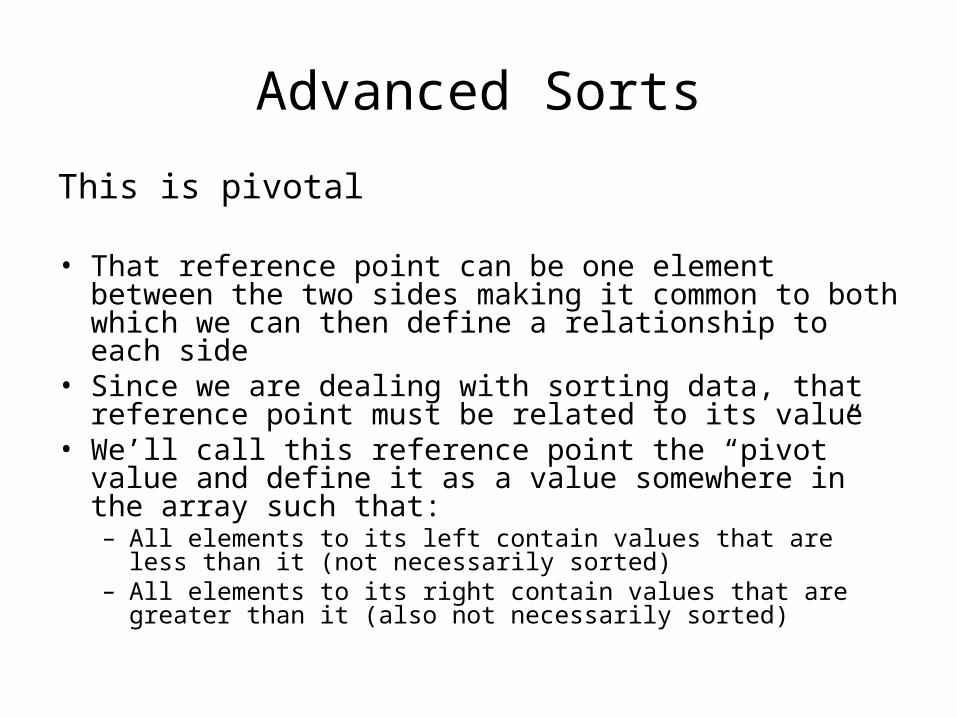
• That reference point can be one element between the two sides making it common to both which we can then define a relationship to each side

• Since we are dealing with sorting data, that reference point must be related to its value

• We’ll call this reference point the “pivot” value and define it as a value somewhere in the array such that:– All elements to its left contain values that are less than it

(not necessarily sorted)– All elements to its right contain values that are greater

than it (also not necessarily sorted)

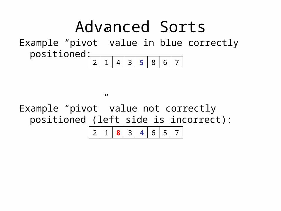
Advanced SortsExample “pivot” value in blue correctly positioned:

Example “pivot” value not correctly positioned (left side is incorrect):

2 4 3 5 8 6 71

2 8 3 4 6 5 71

Advanced Sorts

Staging the data

• Why is this relationship between sides and a pivot value important?

• It gives us a way to express splitting the array that we can approach recursively

• As we did with the mergesort, we can then split the array into smaller pieces until it’s time to stop

• What is the stopping point? Recall that with the mergesort, the base case was when the array splitting came down to 1 element left, which by definition is a sorted sub array

• The same can apply here except that instead of merging two sorted sub arrays, we split the array into sub arrays that repeatedly maintain this pivot-to-sides relationship

• So now the question is, how do we create sub arrays that are correctly positioned around a pivot value? How do we even choose the pivot value?

Advanced Sorts

Partitioning

• That process we will call “partitioning” and like the merge function in mergesort, this sorting algorithm will use the partition function in its recursive case

• The idea is then to repeatedly partition the array and its sub parts recursively until there is nothing necessary to partition

• By the time you are done partitioning to the smallest subarrays, the entire array should be sorted

• So how do we partition an array? Here’s the algorithm

Advanced Sorts

Partitioning

• Select an arbitrary element, such as the last element in the current part of the array – its value will represent the pivot value for the partition

• Go to the first element in the array and examine elements from left to right until you find a value that is greater than or equal to the pivot value – call this the left index point

• Repeat the process from the last element (which is the first element left of the pivot), this time going right to left until you find a value less than the pivot value or you’ve passed the beginning of the array – this is the right index point

• When both loops have stopped, they index pointers will be in 1 of 2 situations:– The “left” and “right” index pointers did not cross paths– The “left” and “right” index pointers crossed paths (including being at

the same spot)

Advanced SortsStarting point. Pivot will be the value in blue:

4 7 5 3 2 8 61

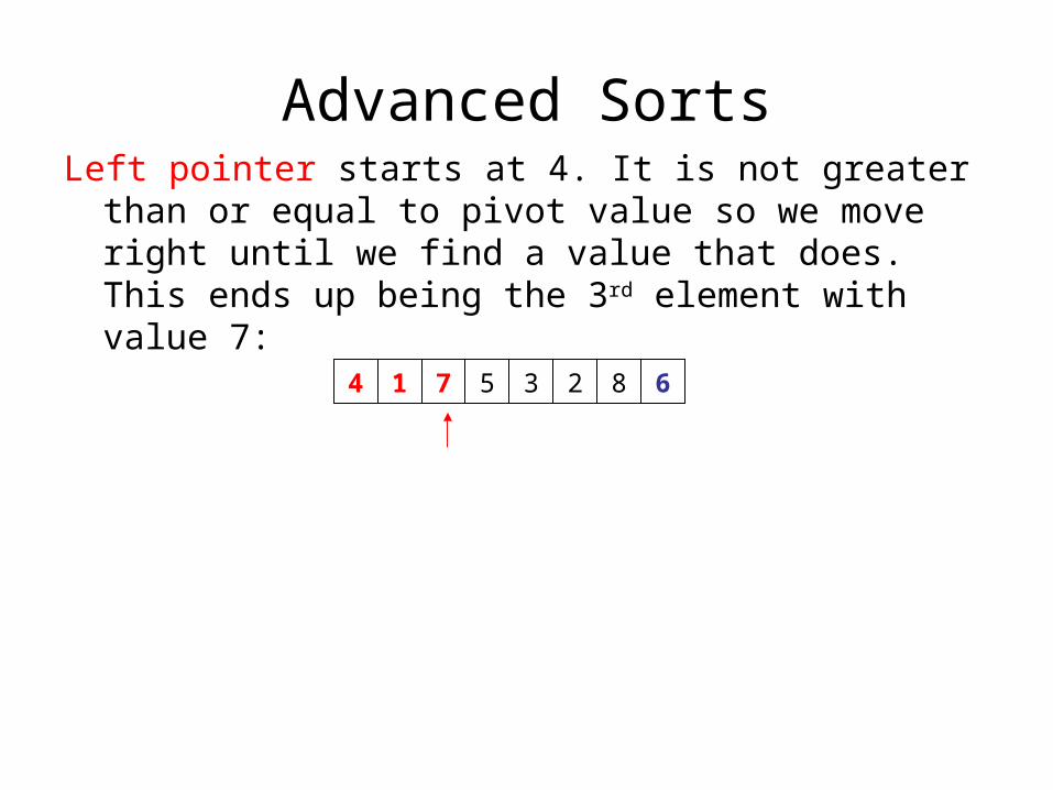
Advanced SortsLeft pointer starts at 4. It is not greater than or

equal to pivot value so we move right until we find a value that does. This ends up being the 3rd element with value 7:

4 7 5 3 2 8 61

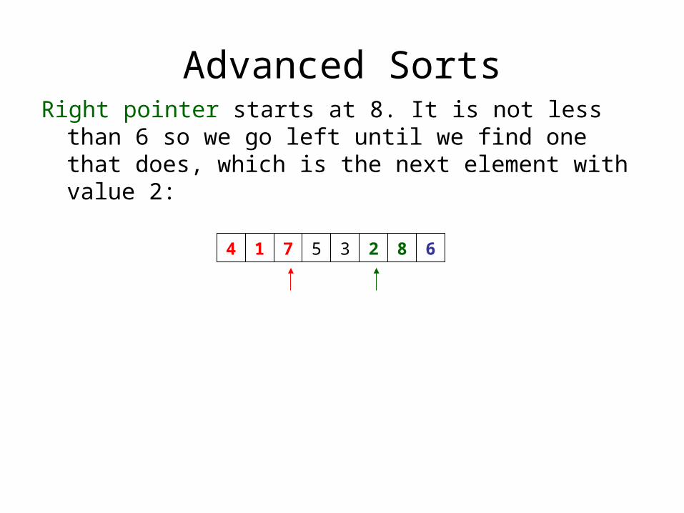
Advanced SortsRight pointer starts at 8. It is not less than 6 so we

go left until we find one that does, which is the next element with value 2:

4 7 5 3 2 8 61

Advanced Sorts

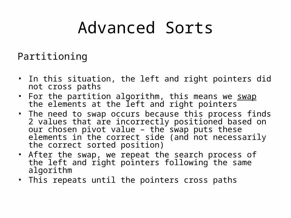
Partitioning

• In this situation, the left and right pointers did not cross paths

• For the partition algorithm, this means we swap the elements at the left and right pointers

• The need to swap occurs because this process finds 2 values that are incorrectly positioned based on our chosen pivot value – the swap puts these elements in the correct side (and not necessarily the correct sorted position)

• After the swap, we repeat the search process of the left and right pointers following the same algorithm

• This repeats until the pointers cross paths

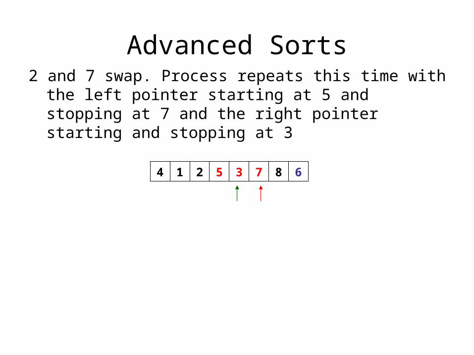
Advanced Sorts2 and 7 swap. Process repeats this time with the left

pointer starting at 5 and stopping at 7 and the right pointer starting and stopping at 3

4 2 5 3 7 8 61

Advanced Sorts

Partitioning

• In this situation, the left and right pointers have crossed paths

• Now, the elements at the left and right pointers do not swap positions with each other

• Instead, the location of the left index pointer becomes, shall we say, “pivotal”

• Notice that the left pointer’s location ends up being the location where the pivot value should go

• Also notice that, by logical rule, the value at the left pointer’s location belongs on the right side

• There is only one value on the right side of where the pivot value should be that is incorrectly positioned – it’s the pivot element itself! Thus, we swap left pointer with pivot

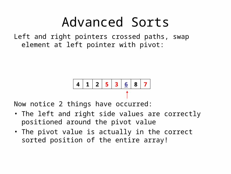
Advanced SortsLeft and right pointers crossed paths, swap element at

left pointer with pivot:

Now notice 2 things have occurred:• The left and right side values are correctly positioned

around the pivot value• The pivot value is actually in the correct sorted

position of the entire array!

4 2 5 3 6 8 71

Advanced Sorts

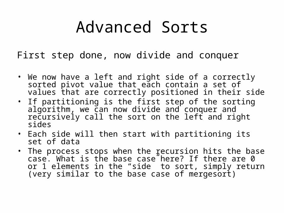
First step done, now divide and conquer

• We now have a left and right side of a correctly sorted pivot value that each contain a set of values that are correctly positioned in their side

• If partitioning is the first step of the sorting algorithm, we can now divide and conquer and recursively call the sort on the left and right sides

• Each side will then start with partitioning its set of data• The process stops when the recursion hits the base case.

What is the base case here? If there are 0 or 1 elements in the “side” to sort, simply return (very similar to the base case of mergesort)

Advanced Sorts

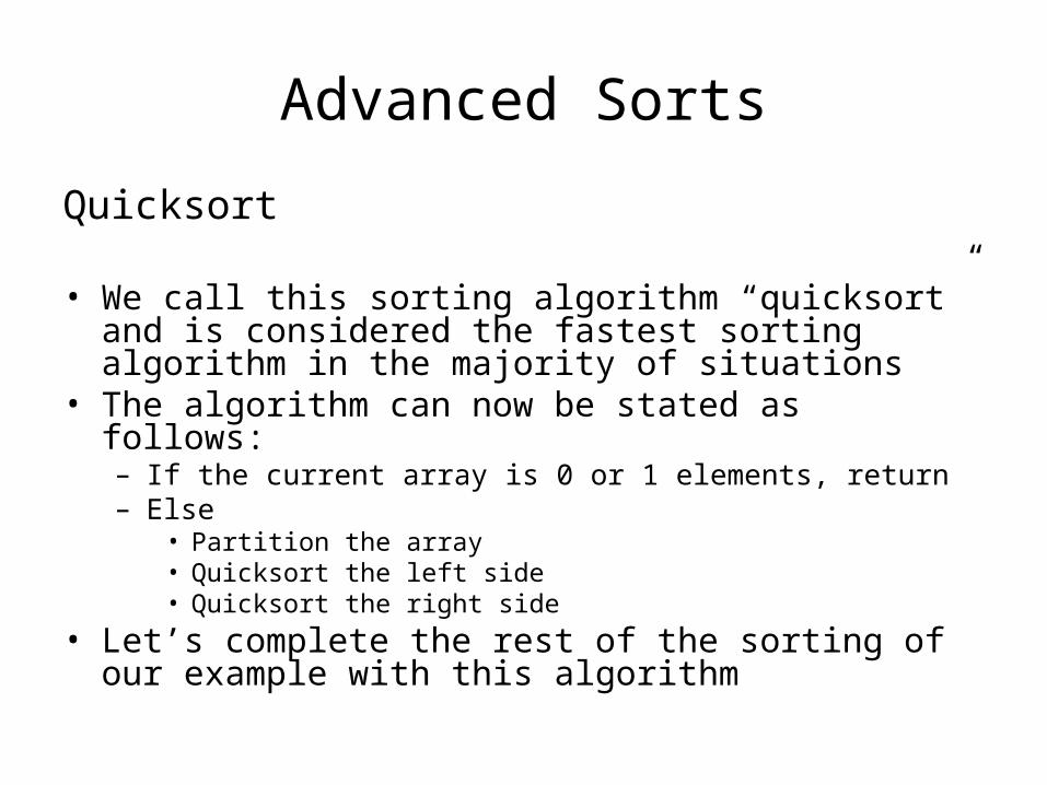
Quicksort

• We call this sorting algorithm “quicksort” and is considered the fastest sorting algorithm in the majority of situations

• The algorithm can now be stated as follows:– If the current array is 0 or 1 elements, return– Else

• Partition the array• Quicksort the left side• Quicksort the right side

• Let’s complete the rest of the sorting of our example with this algorithm

Advanced SortsQuicksort left side (0..4). It’s not the base case so

we partition. Pivot value is 3. Left and right pointers get ready to do their work

4 2 5 3 6 8 71

Advanced SortsLeft stops at 4 (it is greater than 3) and right stops

at 2 (5 was greater than 3, but not 2). The pointers do not cross paths so the two elements will swap

4 2 5 3 6 8 71

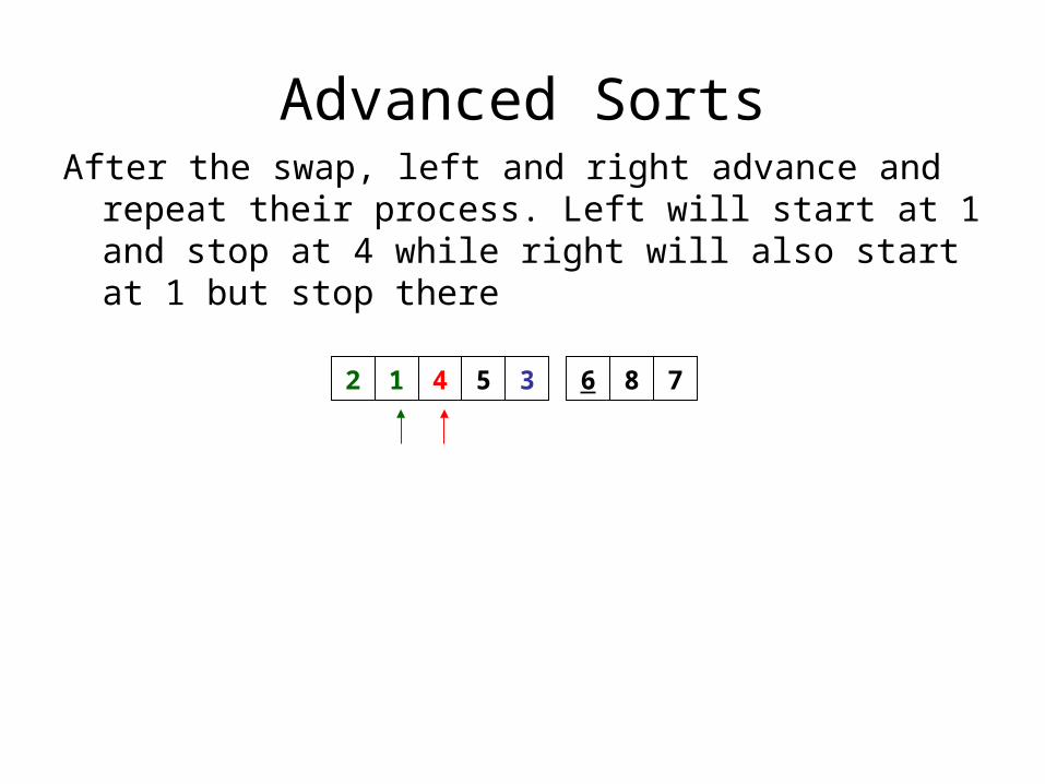
Advanced SortsAfter the swap, left and right advance and repeat

their process. Left will start at 1 and stop at 4 while right will also start at 1 but stop there

2 4 5 3 6 8 71

Advanced SortsLeft and right have crossed paths. Left is in the

correct pivot position and we swap it with pivot. 3 is in the correct sorted position and its left and right sides are correctly partitioned

2 3 5 4 6 8 71

Advanced SortsWe are still in Quicksort(0..4) and just partitioned it.

Now we Quicksort its left and right sides, starting with Quicksort (0..1)

2 3 5 4 6 8 71

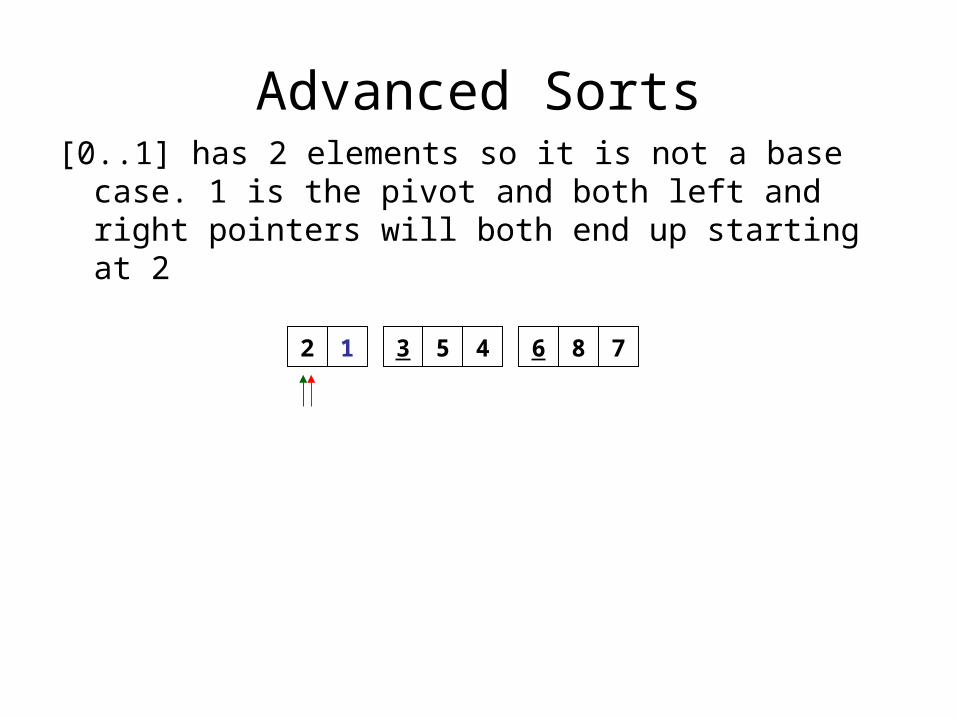
Advanced Sorts[0..1] has 2 elements so it is not a base case. 1 is

the pivot and both left and right pointers will both end up starting at 2

2 3 5 4 6 8 71

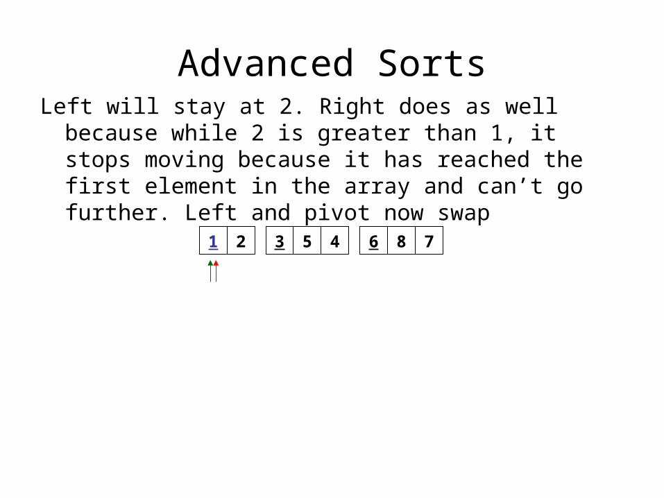
Advanced SortsLeft will stay at 2. Right does as well because while

2 is greater than 1, it stops moving because it has reached the first element in the array and can’t go further. Left and pivot now swap

1 3 5 4 6 8 72

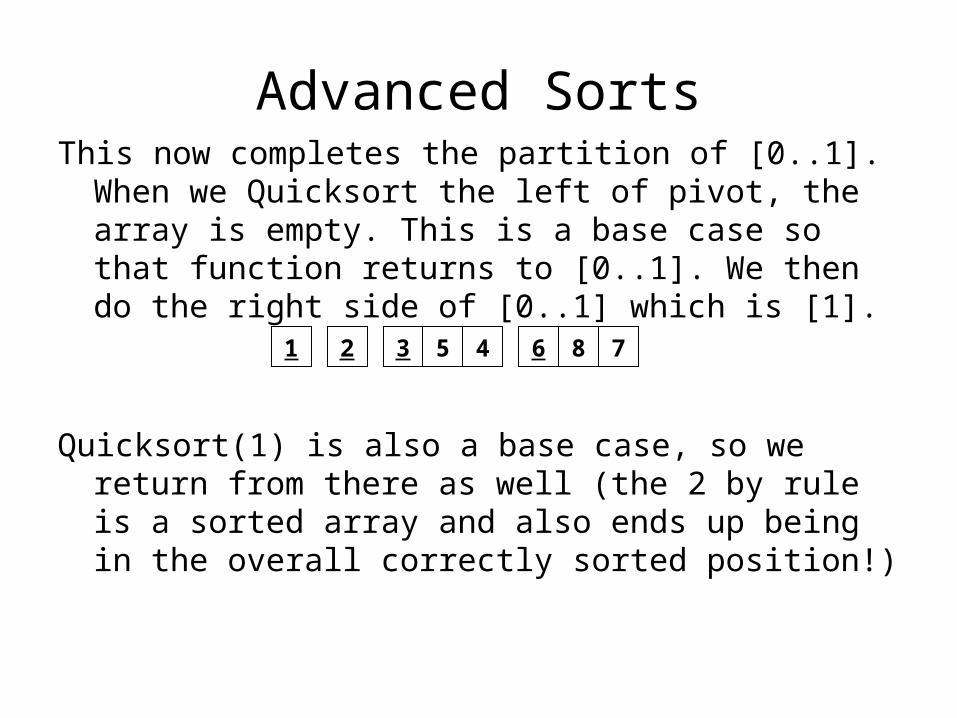
Advanced SortsThis now completes the partition of [0..1]. When we

Quicksort the left of pivot, the array is empty. This is a base case so that function returns to [0..1]. We then do the right side of [0..1] which is [1].

Quicksort(1) is also a base case, so we return from there as well (the 2 by rule is a sorted array and also ends up being in the overall correctly sorted position!)

1 3 5 4 6 8 72

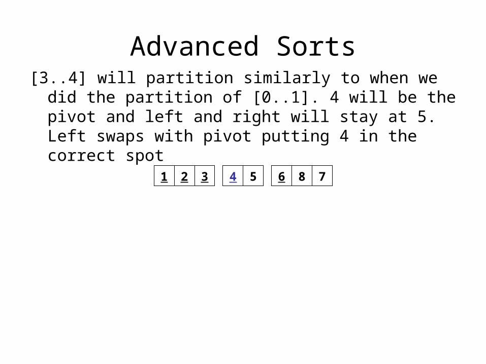
Advanced Sorts[3..4] will partition similarly to when we did the

partition of [0..1]. 4 will be the pivot and left and right will stay at 5. Left swaps with pivot putting 4 in the correct spot

1 3 4 5 6 8 72

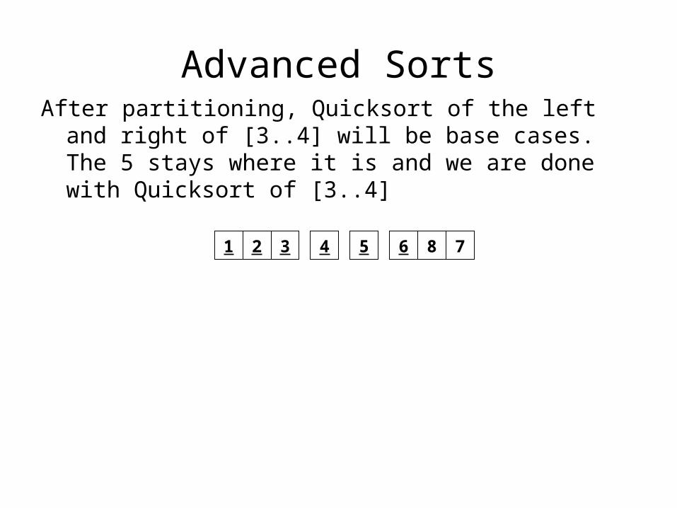
Advanced SortsAfter partitioning, Quicksort of the left and right of

[3..4] will be base cases. The 5 stays where it is and we are done with Quicksort of [3..4]

1 3 4 5 6 8 72

Advanced SortsWe’re back to the overall array of Quicksort [0..7]!

When we left here, we had partitioned around [5] and did Quicksort [0..4]. Now we Quicksort the right side which is [6..7]

1 3 4 5 6 8 72

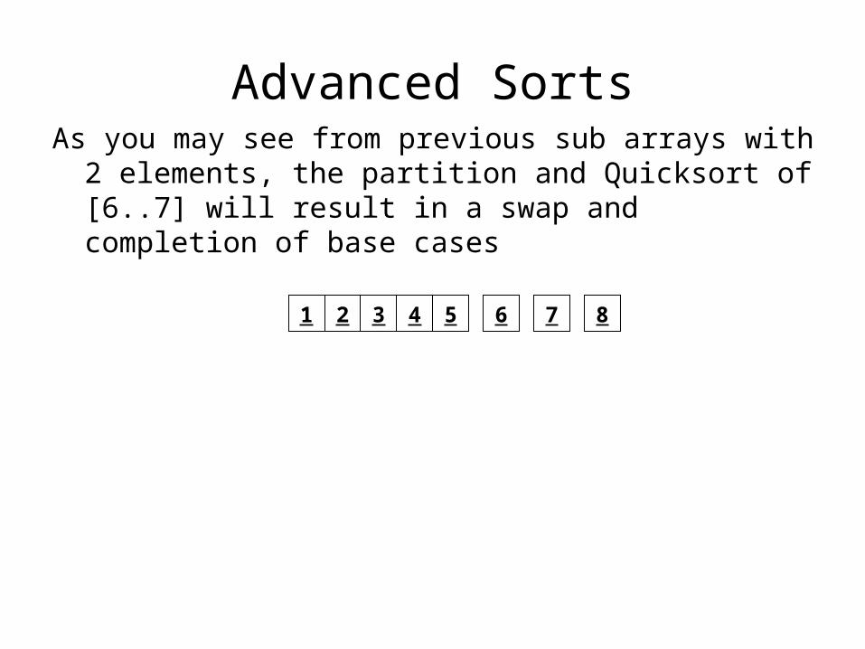
Advanced SortsAs you may see from previous sub arrays with 2

elements, the partition and Quicksort of [6..7] will result in a swap and completion of base cases

1 3 4 5 6 7 82

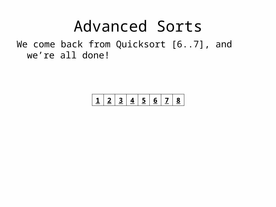
Advanced SortsWe come back from Quicksort [6..7], and we’re all

done!

1 3 4 5 6 7 82

Advanced Sorts

Analysis

• The Quicksort is the same process as the Mergesort except that instead of doing the recursive calls first and then do the merge, we partition first and then do the recursive calls

• Both algorithms use a divide and conquer approach implying that the performance will also be O(n log n)

• This is great news because this algorithm does not use a temp array and thus, does not require twice the memory space to run!

• The worst case situation, though, is not particularly good for Quicksort. Can you spot what it is?

• Before getting into the efficiency of this and all the sort algorithms, let’s take a look at the code

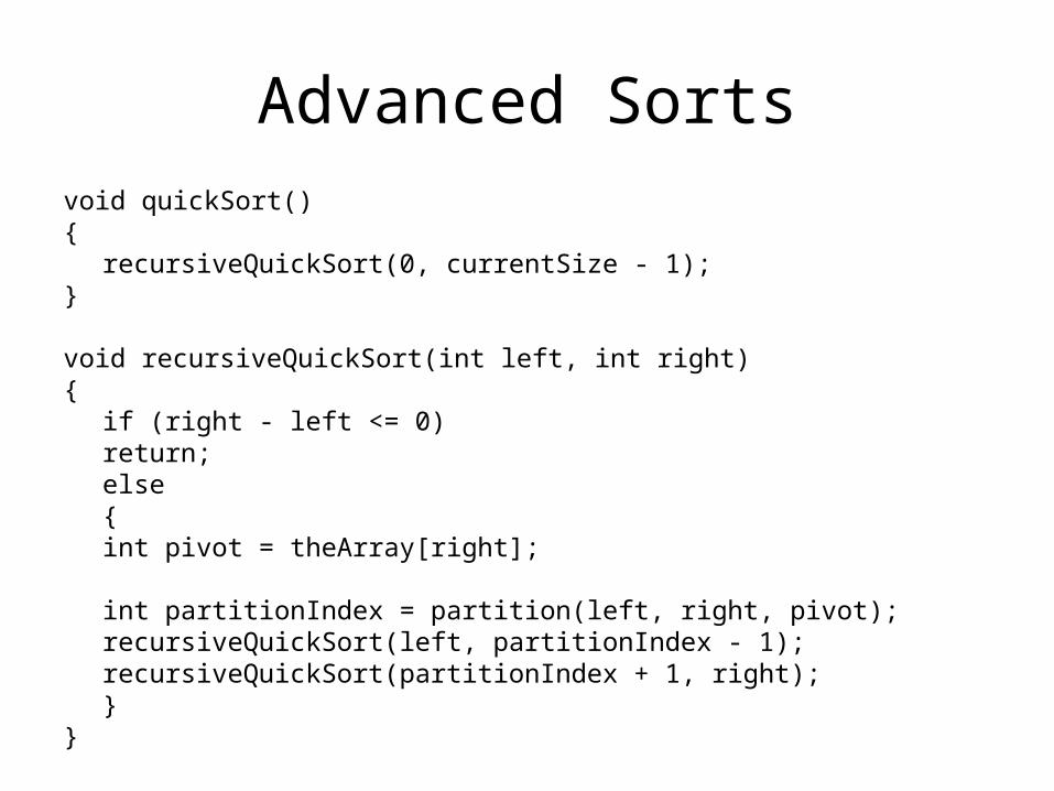
Advanced Sortsvoid quickSort(){

recursiveQuickSort(0, currentSize - 1);}

void recursiveQuickSort(int left, int right){

if (right - left <= 0)return;

else{

int pivot = theArray[right];

int partitionIndex = partition(left, right, pivot);

recursiveQuickSort(left, partitionIndex - 1);recursiveQuickSort(partitionIndex + 1, right);

}}

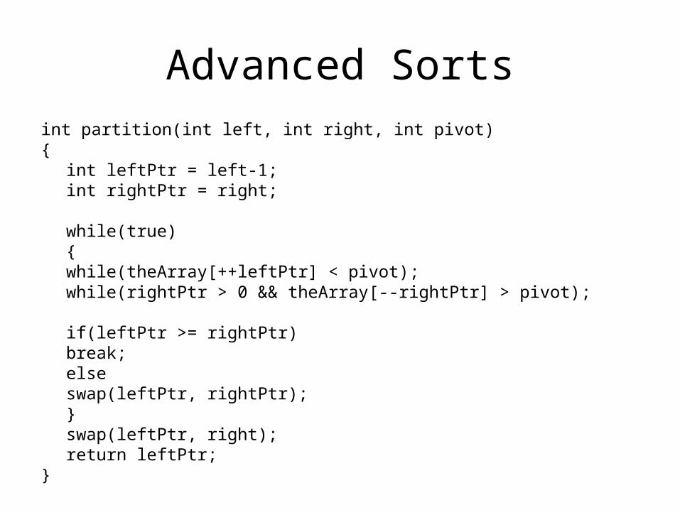
Advanced Sortsint partition(int left, int right, int pivot){

int leftPtr = left-1;int rightPtr = right;

while(true){

while(theArray[++leftPtr] < pivot);while(rightPtr > 0 && theArray[--rightPtr] >

pivot);

if(leftPtr >= rightPtr)break;

elseswap(leftPtr, rightPtr);

}swap(leftPtr, right);return leftPtr;

}

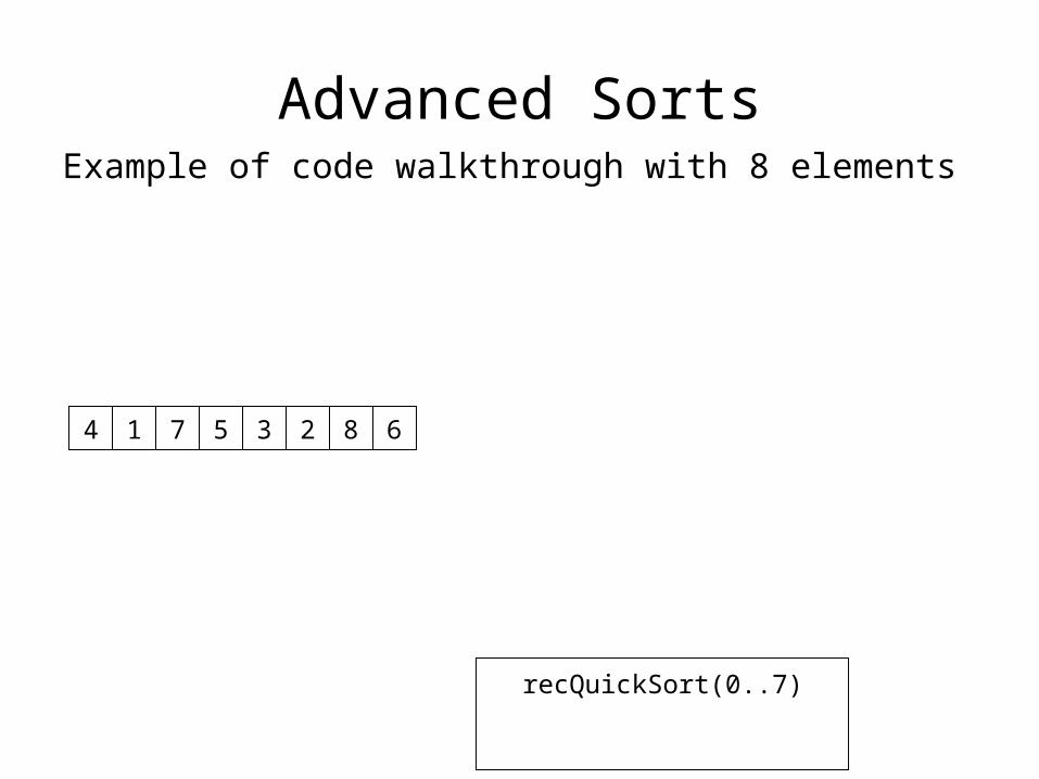
Advanced SortsExample of code walkthrough with 8 elements

recQuickSort(0..7)

4 7 5 3 2 8 61

Advanced Sorts1st call is not a base case, so we partition and then

make the recursive calls. Partition starts with selecting 6

recQuickSort(0..7)

partition(0, 7, 6);

4 7 5 3 2 8 61

Advanced SortsFirst loop starts left index at 0 and stops when left

reaches index 2 because the value found (7) is greater than pivot

recQuickSort(0..7)

partition(0, 7, 6);

4 7 5 3 2 8 61

partition(0, 7, 6)

left = 2

Advanced SortsSecond loop starts right index at 6 and stops when

right reaches index 5 because the value found (2) is less than pivot

recQuickSort(0..7)

partition(0, 7, 6);

4 7 5 3 2 8 61

partition(0, 7, 6)

left = 2, right = 5

Advanced SortsLeft is not greater than or equal to right index

pointer (they did not cross paths), so we swap them

recQuickSort(0..7)

partition(0, 7, 6);

4 2 5 3 7 8 61

partition(0, 7, 6)

swap (2, 5);

Advanced SortsThe loops repeat, this time with left starting at

index 3 and stopping at 5. Right goes from 5 to 4

recQuickSort(0..7)

partition(0, 7, 6);

4 2 5 3 7 8 61

partition(0, 7, 6)

left = 5, right = 4

Advanced SortsLeft is greater than right (they have crossed paths),

so the loops stop and we swap where left index is with the pivot element

recQuickSort(0..7)

partition(0, 7, 6);

4 2 5 3 6 8 71

partition(0, 7, 6)

swap (5, 7);

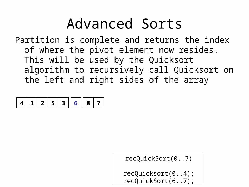
Advanced SortsPartition is complete and returns the index of where

the pivot element now resides. This will be used by the Quicksort algorithm to recursively call Quicksort on the left and right sides of the array

recQuickSort(0..7)

partitionIndex = 5;

4 2 5 3 6 8 71

5

Advanced SortsPartition is complete and returns the index of where

the pivot element now resides. This will be used by the Quicksort algorithm to recursively call Quicksort on the left and right sides of the array

recQuickSort(0..7)

recQuicksort(0..4);recQuickSort(6..7);

4 2 5 3 6 8 71

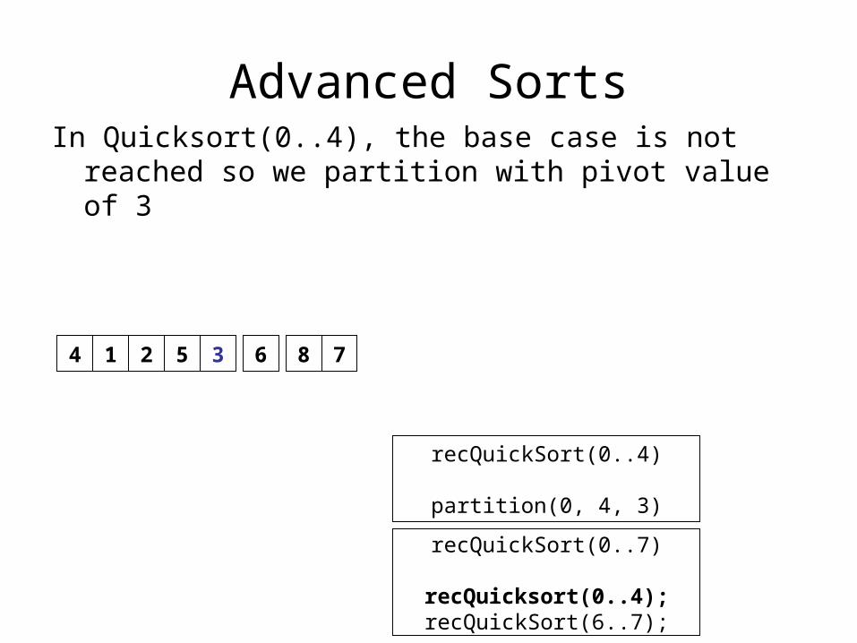
Advanced SortsIn Quicksort(0..4), the base case is not reached so

we partition with pivot value of 3

recQuickSort(0..7)

recQuicksort(0..4);recQuickSort(6..7);

4 2 5 3 6 8 71

recQuickSort(0..4)

partition(0, 4, 3)

Advanced SortsThe loops begin with left index starting and

stopping at 0 and right starting at 3 and stopping at 2

recQuickSort(0..7)

recQuicksort(0..4);recQuickSort(6..7);

4 2 5 3 6 8 71

recQuickSort(0..4)

partition(0, 4, 3)

partition(0, 4, 3)

left = 0, right = 2

Advanced SortsLeft and right did not cross paths, so they swap

recQuickSort(0..7)

recQuicksort(0..4);recQuickSort(6..7);

2 4 5 3 6 8 71

recQuickSort(0..4)

partition(0, 4, 3)

partition(0, 4, 3)

swap(0, 2);

Advanced SortsLoops repeat with left starting at 1 and stopping at

2 and right starting and stopping at 1

recQuickSort(0..7)

recQuicksort(0..4);recQuickSort(6..7);

2 4 5 3 6 8 71

recQuickSort(0..4)

partition(0, 4, 3)

partition(0, 4, 3)

left = 2, right = 1

Advanced SortsLeft and right have crossed paths, so the loops stop

and left swaps with pivot

recQuickSort(0..7)

recQuicksort(0..4);recQuickSort(6..7);

2 3 5 4 6 8 71

recQuickSort(0..4)

partition(0, 4, 3)

partition(0, 4, 3)

swap(2, 4);

Advanced SortsThe partition is complete and returns pivot index of

2. This is used to split [0..4] and recursively call Quicksort on the sides

recQuickSort(0..7)

recQuicksort(0..4);recQuickSort(6..7);

2 3 5 4 6 8 71

recQuickSort(0..4)

recQuickSort(0..1);recQuickSort(3..4);

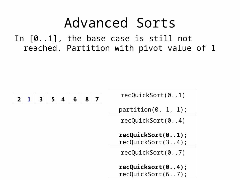
Advanced SortsIn [0..1], the base case is still not reached. Partition

with pivot value of 1

recQuickSort(0..7)

recQuicksort(0..4);recQuickSort(6..7);

2 3 5 4 6 8 71

recQuickSort(0..4)

recQuickSort(0..1);recQuickSort(3..4);

recQuickSort(0..1)

partition(0, 1, 1);

Advanced SortsLeft starts and stops at 0 and right starts at 0 and

ends at -1

recQuickSort(0..7)

recQuicksort(0..4);recQuickSort(6..7);

2 3 5 4 6 8 71

recQuickSort(0..4)

recQuickSort(0..1);recQuickSort(3..4);

recQuickSort(0..1)

partition(0, 1, 1);

partition(0, 1, 1)

left = 0, right = -1

Advanced SortsLeft and right start out crossing paths. Swap with

left and pivot

recQuickSort(0..7)

recQuicksort(0..4);recQuickSort(6..7);

1 3 5 4 6 8 72

recQuickSort(0..4)

recQuickSort(0..1);recQuickSort(3..4);

recQuickSort(0..1)

partition(0, 1, 1);

partition(0, 1, 1)

swap(0, 1);

Advanced SortsPartition index returned to [0..1] is 0. The recursive

calls are next, and these will be quick because they are both base cases that will simply return

recQuickSort(0..7)

recQuicksort(0..4);recQuickSort(6..7);

1 3 5 4 6 8 72

recQuickSort(0..4)

recQuickSort(0..1);recQuickSort(3..4);

recQuickSort(0..1)

recQuickSort(-1);recQuickSort(1);

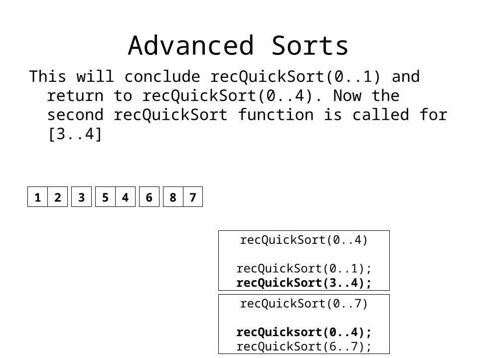
Advanced SortsThis will conclude recQuickSort(0..1) and return to

recQuickSort(0..4). Now the second recQuickSort function is called for [3..4]

recQuickSort(0..7)

recQuicksort(0..4);recQuickSort(6..7);

1 3 5 4 6 8 72

recQuickSort(0..4)

recQuickSort(0..1);recQuickSort(3..4);

Advanced SortsIn [3..4], the base case is not reached so we

partition with pivot value 4

recQuickSort(0..7)

recQuicksort(0..4);recQuickSort(6..7);

1 3 5 4 6 8 72

recQuickSort(0..4)

recQuickSort(0..1);recQuickSort(3..4);

recQuickSort(3..4)

partition(3, 4, 4);

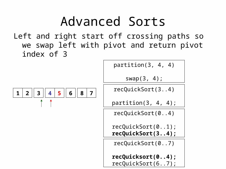
Advanced SortsLeft and right start off crossing paths so we swap

left with pivot and return pivot index of 3

recQuickSort(0..7)

recQuicksort(0..4);recQuickSort(6..7);

1 3 4 5 6 8 72

recQuickSort(0..4)

recQuickSort(0..1);recQuickSort(3..4);

recQuickSort(3..4)

partition(3, 4, 4);

partition(3, 4, 4)

swap(3, 4);

Advanced SortsThe next 2 recursive calls in [3..4] will be base

cases that simply return. When they come back, we can return from recQuickSort(3..4)

recQuickSort(0..7)

recQuicksort(0..4);recQuickSort(6..7);

1 3 4 5 6 8 72

recQuickSort(0..4)

recQuickSort(0..1);recQuickSort(3..4);

recQuickSort(3..4)

recQuickSort(2);recQuickSort(4);

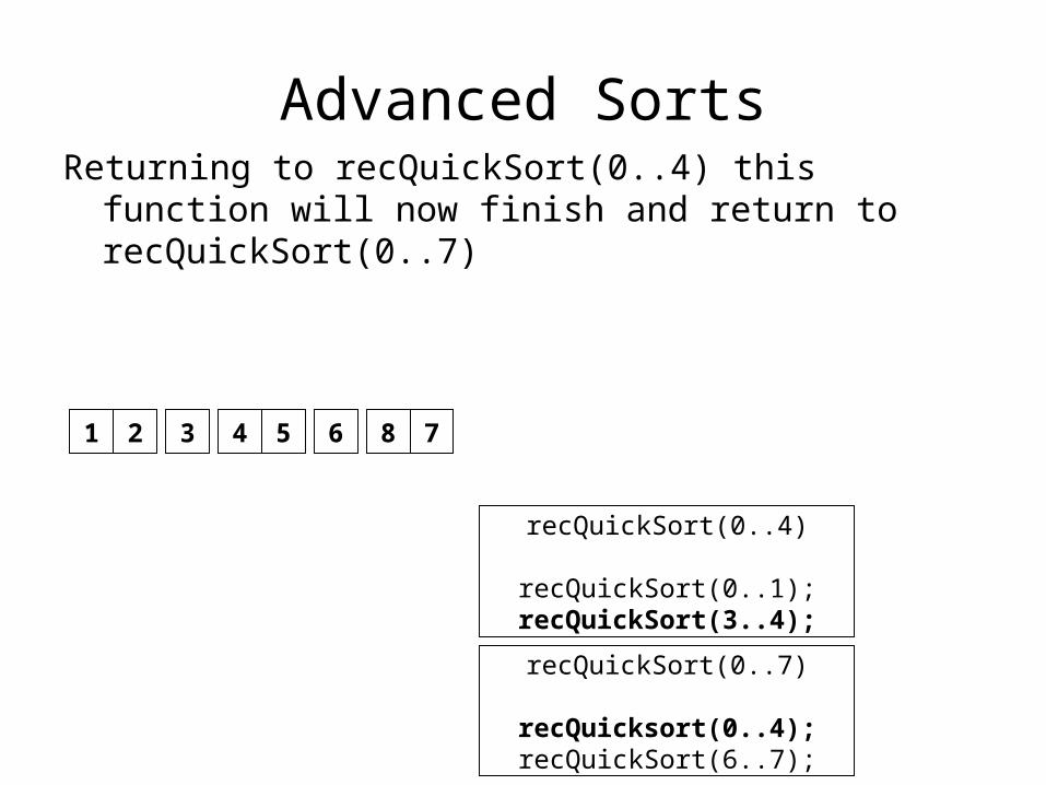
Advanced SortsReturning to recQuickSort(0..4) this function will

now finish and return to recQuickSort(0..7)

recQuickSort(0..7)

recQuicksort(0..4);recQuickSort(6..7);

1 3 4 5 6 8 72

recQuickSort(0..4)

recQuickSort(0..1);recQuickSort(3..4);

Advanced SortsReturning to recQuickSort(0..4) this function will

now finish and return to recQuickSort(0..7)

recQuickSort(0..7)

recQuicksort(0..4);recQuickSort(6..7);

1 3 4 5 6 8 72

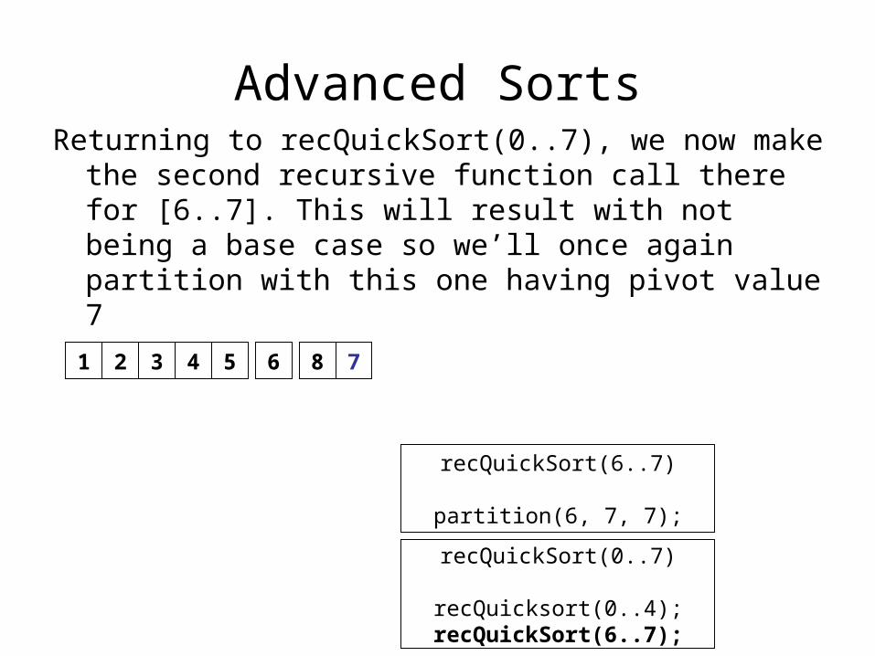
Advanced SortsReturning to recQuickSort(0..7), we now make the

second recursive function call there for [6..7]. This will result with not being a base case so we’ll once again partition with this one having pivot value 7

recQuickSort(0..7)

recQuicksort(0..4);recQuickSort(6..7);

1 3 4 5 6 8 72

recQuickSort(6..7)

partition(6, 7, 7);

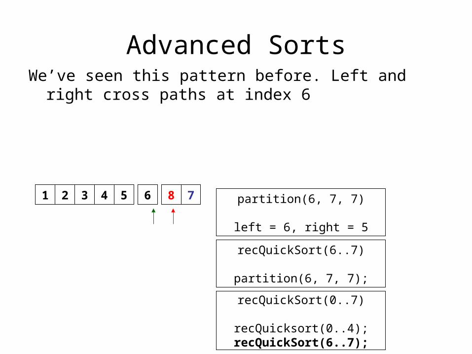
Advanced SortsWe’ve seen this pattern before. Left and right cross

paths at index 6

recQuickSort(0..7)

recQuicksort(0..4);recQuickSort(6..7);

1 3 4 5 6 8 72

recQuickSort(6..7)

partition(6, 7, 7);

partition(6, 7, 7)

left = 6, right = 5

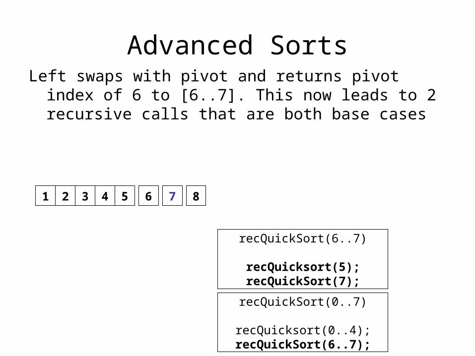
Advanced SortsLeft swaps with pivot and returns pivot index of 6 to

[6..7]. This now leads to 2 recursive calls that are both base cases

recQuickSort(0..7)

recQuicksort(0..4);recQuickSort(6..7);

1 3 4 5 6 7 82

recQuickSort(6..7)

recQuicksort(5);recQuickSort(7);

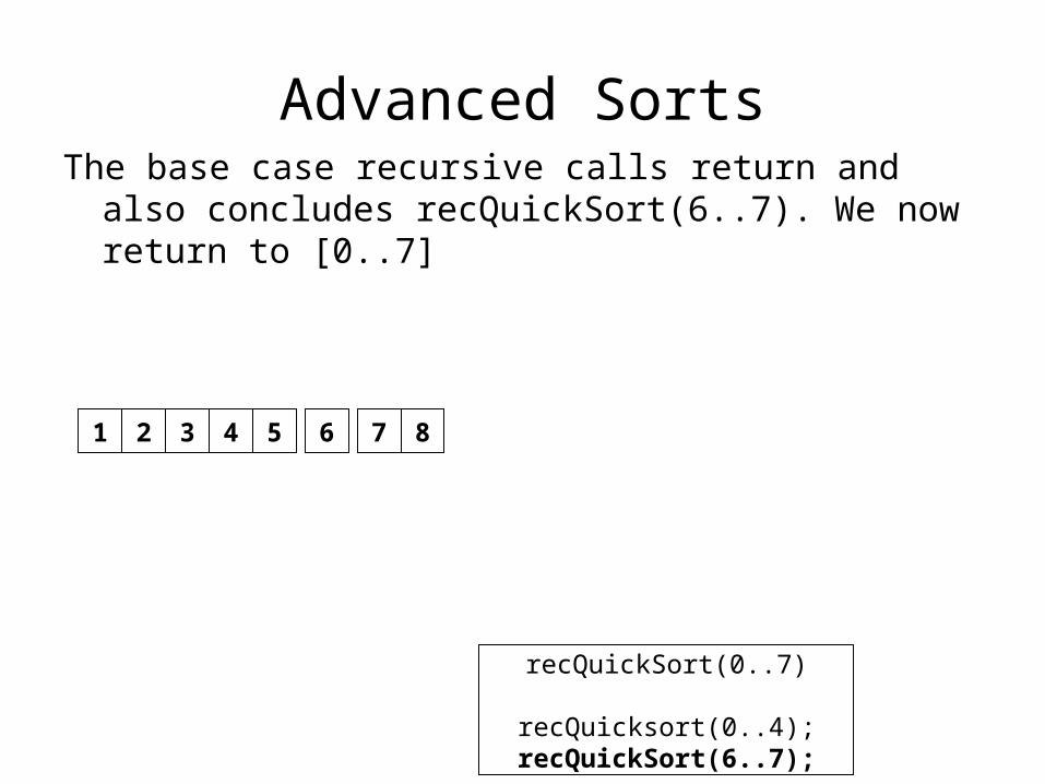
Advanced SortsThe base case recursive calls return and also

concludes recQuickSort(6..7). We now return to [0..7]

recQuickSort(0..7)

recQuicksort(0..4);recQuickSort(6..7);

1 3 4 5 6 7 82

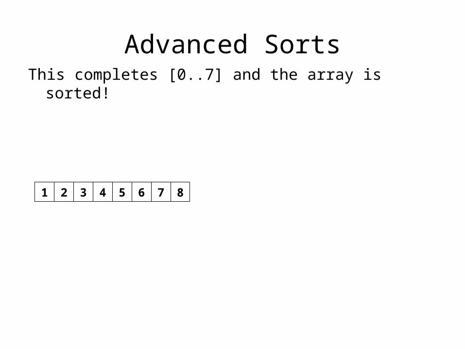
Advanced SortsThis completes [0..7] and the array is sorted!

1 3 4 5 6 7 82

Advanced Sorts

Efficiency

• Like Mergesort, Quicksort follows the divide and conquer recursive method along with a key operation (the partition)

• The partition performs at O(n) per level of array splits like the merge function in Mergesort. The splitting of the array to perform the recursion performs at O(log n)

• Thus, the performance of Quicksort is O(n log n)• The biggest key difference is the unnecessary need for a

temp array with Quicksort, so already there is a strong advantage with Quicksort over Mergesort

• Putting space usage aside, do the comparisons alone make a difference between the 2 algorithms?

Advanced Sorts

Mergesort vs. Quicksort

• Mergesort compares will be much more consistent with performance over quicksort– The merge portion performs 3 compares until one sub array is

complete – this goes at about O(n/2) – The remaining elements are linearly inserted into temp for the

remaining O(n/2)– There is also a loop to copy the temp workspace back into theArray

which is another O(n)– Overall compares for the merge function is category O(n), but more

detailed at around O(5n/2)• Quicksort number of compares are not based on performing

actions until a sub array is complete, but involves the state of the data – some partitions will involve more compares than others

• This implies that there are best and worst case situations with Quicksort

Advanced Sorts

Mergesort vs. Quicksort

• What’s a good partition? When the pivot value is one that ends up being near the middle of the array

• Best case:Turns out that the more random the distribution, the better the performance because the chance is increased for a pivot value that belongs in the middle of the array

• Worst case: The data is nearly sorted or reverse sorted – the pivot values end up being on the edge of the sub arrays and splits become arrays of size 1 and n-1 – this leads to performance near O(n2)

• Best case situations are more common and better suited for random distribution of data which is O(n log n)

• Partition compares range from O(n) to O(2n) depending on the number of swaps that take place as left and right pointers move

• Partition also does not perform an O(n) copy of temp to theArray• With both Merge and Quick being O(n log n), Quicksort will outperform

Mergesort, as long as worst case situations are avoided

Advanced SortsComparisons Notes

Bubble O(n2)Swaps on average

greater than Selection

Selection O(n2) Swaps are O(n)

Insertion O(n2) (worst case)

Range is O(n) to (n2) Excellent for partially

sorted lists

Merge O(n log n)

Requires 2x memory space because of temp

array

Quick O(n log n)

Faster and more space efficient than Merge, but degrades to O(n2) when

the array is near or reverse sorted

Advanced Sorts

Other ideas

• Other advanced sorts exist:– Shell and Radix sort use a similar divide and conquer approach

performing at O(n log n) – Quicksort on average still wins– Modifications of quicksort to partition or select pivot values differently– Use of insertion sort on sub arrays within the quicksort algorithm to

take advantage of partitions that result in near sorted situations• Back track: the sorting algorithms take place with arrays because

by sorting the data, the search for an element significantly improves from O(n) to O(log n)

• Arrays are static in memory. Linked lists are dynamic, but even if we sort them, we cannot get O(log n) search because the middle of the list cannot be directly accessed…

• …unless we try another structure…