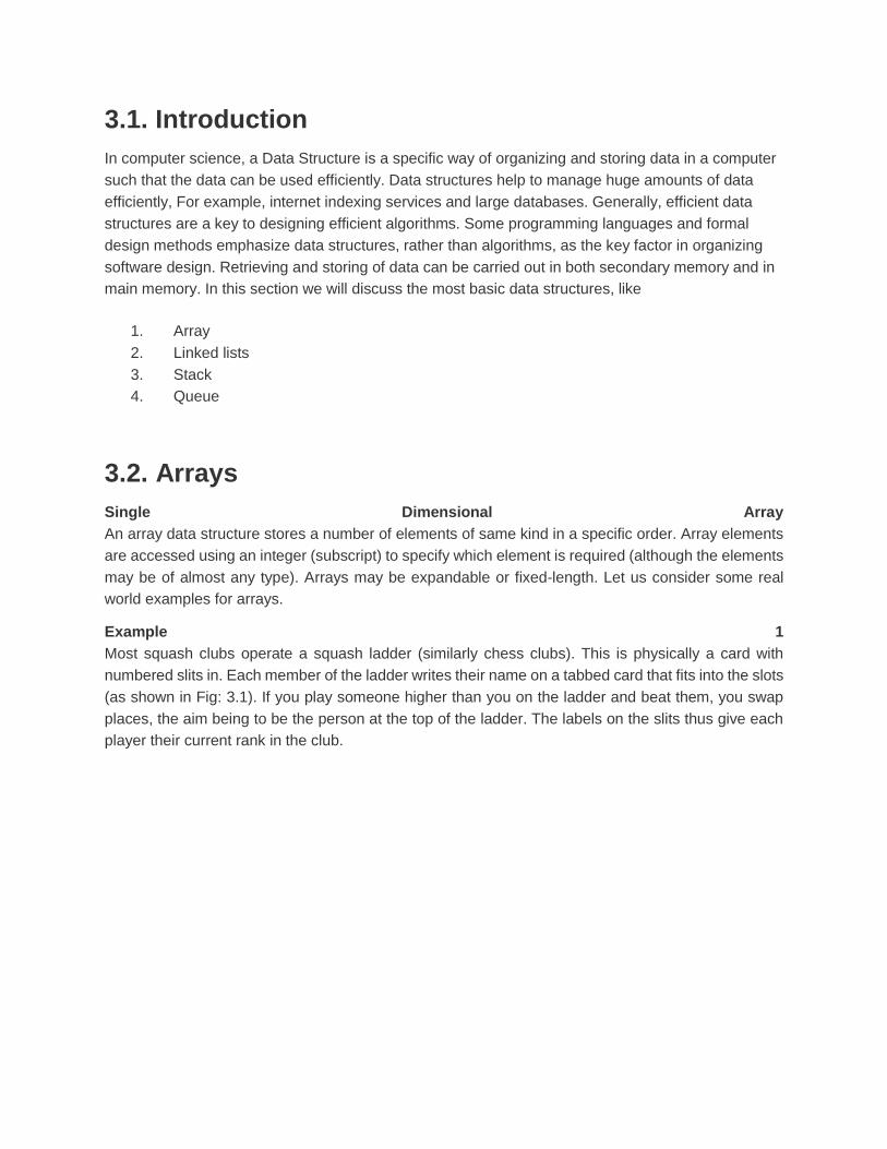
3.1. Introduction

In computer science, a Data Structure is a specific way of organizing and storing data in a computer

such that the data can be used efficiently. Data structures help to manage huge amounts of data

efficiently, For example, internet indexing services and large databases. Generally, efficient data

structures are a key to designing efficient algorithms. Some programming languages and formal

design methods emphasize data structures, rather than algorithms, as the key factor in organizing

software design. Retrieving and storing of data can be carried out in both secondary memory and in

main memory. In this section we will discuss the most basic data structures, like

1. Array

2. Linked lists

3. Stack

4. Queue

3.2. Arrays

Single Dimensional Array

An array data structure stores a number of elements of same kind in a specific order. Array elements

are accessed using an integer (subscript) to specify which element is required (although the elements

may be of almost any type). Arrays may be expandable or fixed-length. Let us consider some real

world examples for arrays.

Example 1

Most squash clubs operate a squash ladder (similarly chess clubs). This is physically a card with

numbered slits in. Each member of the ladder writes their name on a tabbed card that fits into the slots

(as shown in Fig: 3.1). If you play someone higher than you on the ladder and beat them, you swap

places, the aim being to be the person at the top of the ladder. The labels on the slits thus give each

player their current rank in the club.

The squash ladder is an array structure. All the entries are of the same kind: they are all names of

squash players. Each position is numerically labeled, so you can easily ask questions such as, who

the current No 1 is or who is three positions higher than me? The ladder also has a predetermined

number of positions. If there are more people wishing to be on the ladder than there are slots, a waiting

list may be set up, or a second (division) ladder may be created, but the original physical ladder cannot

have new slots added as there is no space. When a new person arrives who is known to be good, a

new slot cannot be created in the middle of the ladder to start them in a position close to their correct

one. The best that could be done if this were required is to shuffle each player down one position to

create a gap. This would be time-consuming.

Example 2

At sports events such as ice-skating (gymnastics and boxing are similar), marks are awarded by a

panel of judges. The judges sit in a line of seats, with the seat labeled by their country. Before

technology took over, the judges would hold up cards with their scores. On the television screen each

skater's scores are given in a row, again with the marks. This is another example of an array- a fixed

size list of things of interest (such as scores) each with a label to identify them (such as the country).

In ice skating scores, the "things" are thus numbers and the labels are letter pairs that indicate the

countries of the judges (as shown in Fig: 3.2).

Example 3

A row of houses down one side of a street is also organized like an array. Each house is labeled by

its postal address: for example 1, 3, 5, 7, etc. assuming it is on the even side of the street in Hyderabad.

When a postman has a letter to deliver, they know where it goes from the number. The number is just

a label; the actual house is the thing it is labeling. In normal circumstances, new houses are not added

in the middle. Once your house is given a number, it is not changed.

A one-dimensional array such as the examples above is in many ways similar to a list. The difference

is that arrays are of fixed sizes, with each cell "named" by a subscript. An array consists of a fixed

number of slots, that things can be put in or taken out of. New slots cannot however be created. Since

each element in the array is referenced by a single subscript, it is called as one-dimensional array.

The below example (Figure : 3.3) tells how a list of marks scored by 10 students in one subject is

represented by a one-dimensional array.

here, the name of the array is "marks". All the elements inside it are integers representing the marks

of the students. Usually an array is indexed as zero-based indexing; i.e. the first element of the array

is indexed by subscript of 0. In the above example (Figure : 3.3),

marks[0] represents the marks obtained by the first student i.e., 70

marks[1] represents the marks obtained by the second student i.e., 30

.

.

marks[9] represents the marks obtained by the 10th student i.e., 45

Multi-dimensional arrays

In addition to one-dimensional arrays, we also have two-dimensional and three-dimensional arrays

where the elements are pointed by two and three subscripts respectively. These will come under the

category of Multi-dimensional arrays, since we require multiple subscripts to refer an element in them.

Two-dimensional arrays

A two-dimensional array data structure stores the elements in a rectangular form i.e., in rows and

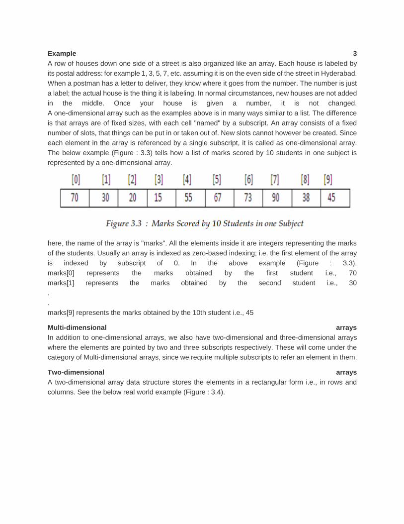
columns. See the below real world example (Figure : 3.4).

If you observe the seating arrangement in a cinema theatre, you will find the seats arranged in rows

and columns. Here, a row is a horizontal list of elements i.e., seats in this example and a column is a

vertical list of elements. To address a seat, we need its row number i.e., in which row it is and it's

column number i.e., in which column it is present.

Example 1

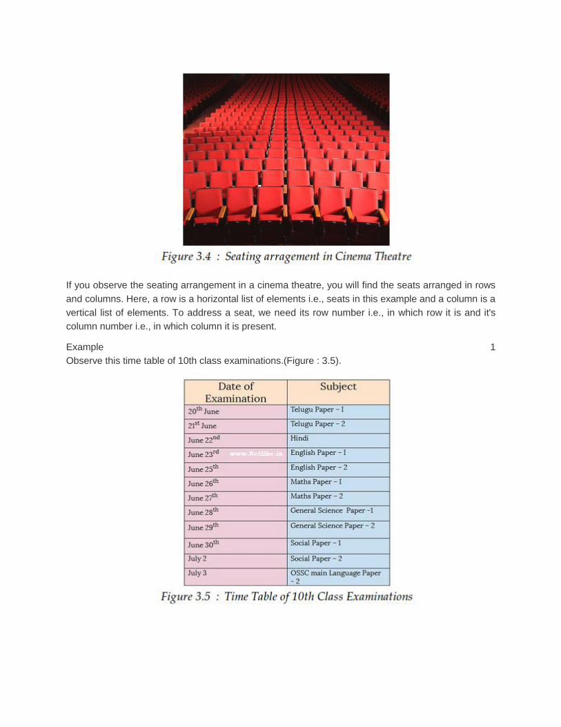
Observe this time table of 10th class examinations.(Figure : 3.5).

Here, 12 different subject's dates are mentioned. In each row, we have two columns for "Date of

examination" and "subject name". One row is providing a date on which test for a specific subject is

going to be conducted. Like this, we have the details for 12 subjects in 12 different rows.

Example 2

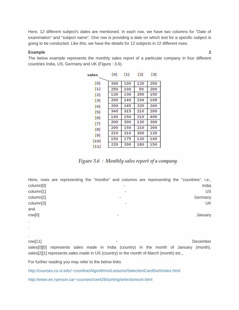
The below example represents the monthly sales report of a particular company in four different

countries India, US, Germany and UK (Figure : 3.6).

Here, rows are representing the "months" and columns are representing the "countries". i.e.,

column[0] - India

column[1] - US

column[2] - Germany

column[3] - UK

and

row[0] - January

.

.

.

row[11] - December

sales[0][0] represents sales made in India (country) in the month of January (month).

sales[2][1] represents sales made in US (country) in the month of March (month) etc.,

For further reading you may refer to the below links

http://courses.cs.vt.edu/~csonline/Algorithms/Lessons/SelectionCardSort/index.html

http://www.ee.ryerson.ca/~courses/coe428/sorting/selectionsort.html

3.3. Linked Lists

Search for a node in the linearly ordered linked list

Problem Statement

Design and implement an algorithm to search a linear ordered linked list for a given alphabetic key or

name.

Algorithm development

With the stack and queue data structures it is always clear in advance exactly where the current item

should be retrieved from or inserted. This favourable situation does not prevail when it is necessary to

perform insertion and deletions on linear linked lists. Before we can carry out such operations with an

ordered linked list we must first carry out a search of the list to establish the position where the change

must be made. It is this problem that we wish to consider in the present discussion. We will need such

a search algorithm later when we come to discuss linked list insertion and deletion operations. Before

starting on the algorithm design let us consider an example that defines the problem we wish to solve.

Suppose we have a long alphabetically ordered list of names as shown in Figure : 3.7 and that we

wish to insert the name DAVID.

The task that must be performed before the insertion can be made is to locate exactly where DAVID

should be inserted. After examining the names list above we quickly respond that DAVID needs to be

inserted between DANIEL and DROVER. At this point, we will not concern ourselves with how the

insertion (or deletion) is made but rather we will concentrate on developing the accompanying search

algorithm for a linked list structure. In deciding where DAVID should be inserted, what we have to do

is search the list until we have either found a name that comes alphabetically later (in the insertion

case) or until we have found a matching name (in the deletion case). On the assumption that the list

is ordered, there will be no need to search further in either case. The central part of our search

algorithm will therefore be:

1. While current search name comes alphabetically after current list name do,

(a) Move to next name in the list.

This algorithm does not take into account that the search name may come after the last name in the

list and as such it is potentially infinite, we will need to take this into account later. Our development

so far has been straightforward and the problem would be almost solved if we only had to search a

linear list rather than a linked linear list. The motivation for maintaining an ordered set of names as a

linked list arises because it allows for efficient insertion and deletion of names while still retaining the

alphabetical order. As we will see later this is certainly not true for a list of names stored as a linear

array. At this point, we are ready to consider the linked list representation of an ordered list and the

accompanying search algorithm.

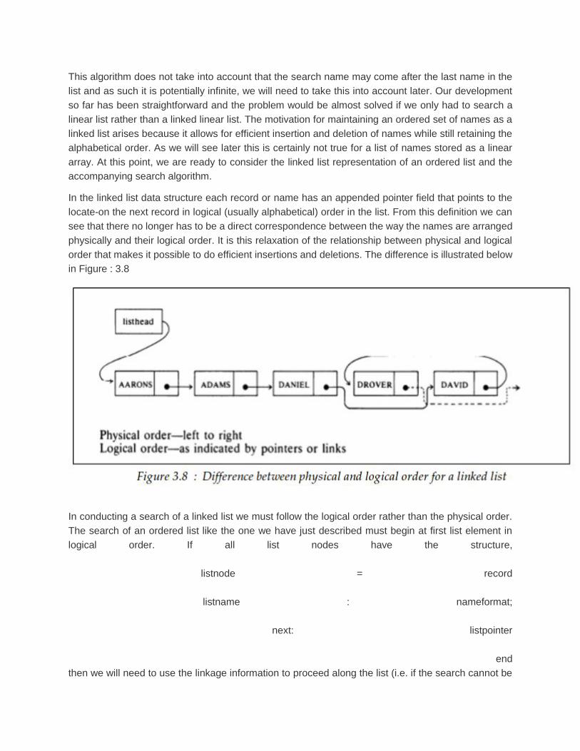
In the linked list data structure each record or name has an appended pointer field that points to the

locate-on the next record in logical (usually alphabetical) order in the list. From this definition we can

see that there no longer has to be a direct correspondence between the way the names are arranged

physically and their logical order. It is this relaxation of the relationship between physical and logical

order that makes it possible to do efficient insertions and deletions. The difference is illustrated below

in Figure : 3.8

In conducting a search of a linked list we must follow the logical order rather than the physical order.

The search of an ordered list like the one we have just described must begin at first list element in

logical order. If all list nodes have the structure,

listnode = record

listname : nameformat;

next: listpointer

end

then we will need to use the linkage information to proceed along the list (i.e. if the search cannot be

terminated at the first element). This will simply amount to assigning the pointer value next in the

current node to the current node pointer, i.e.

current:=next

If we step through the logical order of the list in this manner we will eventually arrive at the desired

position corresponding to the place where the search name either exists or is able to be inserted.

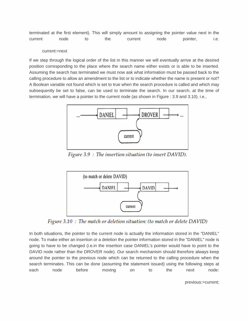
Assuming the search has terminated we must now ask what information must be passed back to the

calling procedure to allow an amendment to the list or to indicate whether the name is present or not?

A Boolean variable not found which is set to true when the search procedure is called and which may

subsequently be set to false, can be used to terminate the search. In our search, at the time of

termination, we will have a pointer to the current node (as shown in Figure : 3.9 and 3.10). i.e.,

In both situations, the pointer to the current node is actually the information stored in the "DANIEL"

node. To make either an insertion or a deletion the pointer information stored in the "DANIEL" node is

going to have to be changed (i.e.in the insertion case DANIEL's pointer would have to point to the

DAVID node rather than the DROVER node). Our search mechanism should therefore always keep

around the pointer to the previous node which can be returned to the calling procedure when the

search terminates. This can be done (assuming the statement issued) using the following steps at

each node before moving on to the next node:

previous:=current;

current:=next;

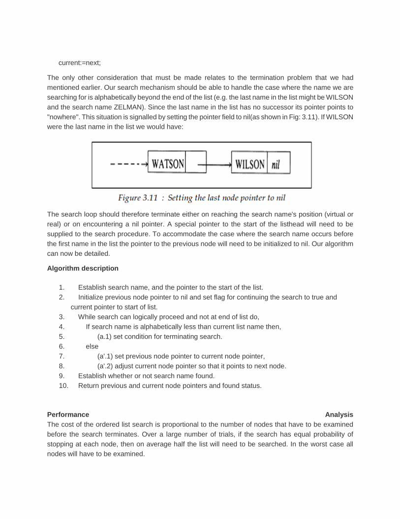
The only other consideration that must be made relates to the termination problem that we had

mentioned earlier. Our search mechanism should be able to handle the case where the name we are

searching for is alphabetically beyond the end of the list (e.g. the last name in the list might be WILSON

and the search name ZELMAN). Since the last name in the list has no successor its pointer points to

"nowhere". This situation is signalled by setting the pointer field to nil(as shown in Fig: 3.11). If WILSON

were the last name in the list we would have:

The search loop should therefore terminate either on reaching the search name's position (virtual or

real) or on encountering a nil pointer. A special pointer to the start of the listhead will need to be

supplied to the search procedure. To accommodate the case where the search name occurs before

the first name in the list the pointer to the previous node will need to be initialized to nil. Our algorithm

can now be detailed.

Algorithm description

1. Establish search name, and the pointer to the start of the list.

2. Initialize previous node pointer to nil and set flag for continuing the search to true and

current pointer to start of list.

3. While search can logically proceed and not at end of list do,

4. If search name is alphabetically less than current list name then,

5. (a.1) set condition for terminating search.

6. else

7. (a'.1) set previous node pointer to current node pointer,

8. (a'.2) adjust current node pointer so that it points to next node.

9. Establish whether or not search name found.

10. Return previous and current node pointers and found status.

Performance Analysis

The cost of the ordered list search is proportional to the number of nodes that have to be examined

before the search terminates. Over a large number of trials, if the search has equal probability of

stopping at each node, then on average half the list will need to be searched. In the worst case all

nodes will have to be examined.

3.4. Stack

Adding (Push) and Deleting (Pop) items from and into the stack

Problem Statement

Implement two algorithms, one for adding items to a stack and the second for removing items from a

stack.

Algorithm development

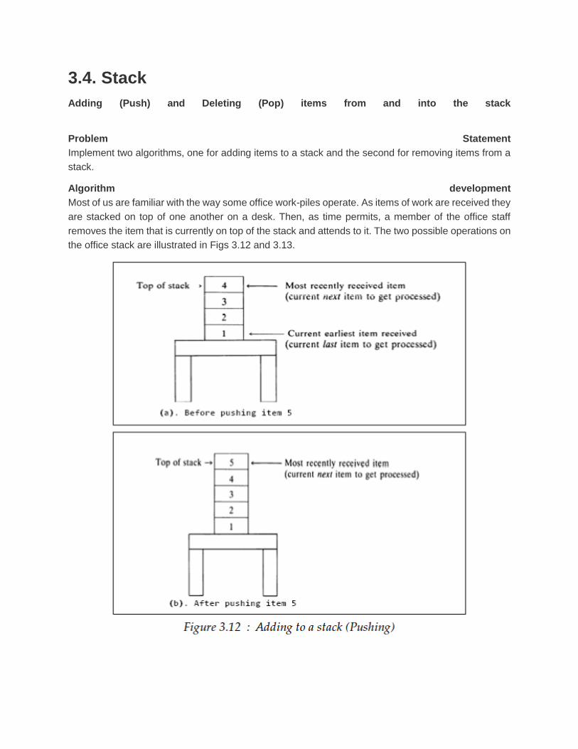
Most of us are familiar with the way some office work-piles operate. As items of work are received they

are stacked on top of one another on a desk. Then, as time permits, a member of the office staff

removes the item that is currently on top of the stack and attends to it. The two possible operations on

the office stack are illustrated in Figs 3.12 and 3.13.

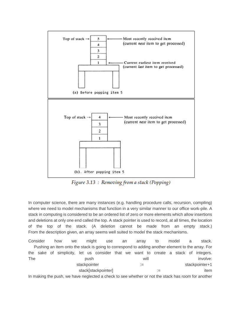
In computer science, there are many instances (e.g. handling procedure calls, recursion, compiling)

where we need to model mechanisms that function in a very similar manner to our office work-pile. A

stack in computing is considered to be an ordered list of zero or more elements which allow insertions

and deletions at only one end called the top. A stack pointer is used to record, at all times, the location

of the top of the stack. (A deletion cannot be made from an empty stack.)

From the description given, an array seems well suited to model the stack mechanisms.

Consider how we might use an array to model a stack.

Pushing an item onto the stack is going to correspond to adding another element to the array. For

the sake of simplicity, let us consider that we want to create a stack of integers.

The push will involve:

stackpointer := stackpointer+1

stack[stackpointer] := item

In making the push, we have neglected a check to see whether or not the stack has room for another

item. After incorporating this check, the implementation of a stack push will be as described below.

push (stack: n elements; stackpointer; item, maxsize);

begin {pushes items onto an array stack}

if stackpointer < maxsize then

begin {push item onto stack}

stackpointer := stackpointer+1;

stack [stackpointer]:= item

end

else

writeln ('stack overflow')

end

Popping an item off the top of the stack is handled just as simply as the push. It amounts to removing

an element from the array. The central steps are:

The push will involve:

item := stack [stackpointer],

stackpointer := stackpointer-1

This time we do not need a check to see if there is overflow but rather a test must be made to see if

there is an item on the stack that can be removed. A Zero value for the stackpointer will signal this

underflow if our array stack has the range [1 .. maxsize]. Implementation for popping from a stack is

therefore as described below.

pop (stack : n elements; item, stackpointer);

begin {pops items from an array stack}

if stackpointer > 0 then

begin {pop item off top of stack}

item := stack[stackpointer]

stackpointer := stack[stackpointer]-1;

end

else

writeln ('stack underflow')

end

We notice in this procedure that when an item is "removed" from the top of the stack it still remains in

the array. However, because of the way in which the stack pointer is used, it is no longer part of the

current stack. Typically in the way in which stacks are used, they may grow and shrink rather

dramatically during the course of execution of a program. These observations highlight a weakness in

using an array to implement a stack. Furthermore, it is sometimes necessary to store large amounts

of information in each stack element. As a consequence, stacks can potentially use up large amounts

of storage.

With the array implementation of a stack, it is necessary to preallocate the maximum stack size at the

time of implementing the program. A much more desirable way to use a stack would be to have it only

take up as much space as there were items on the stack at each point in time during the execution. A

number of programming languages can accommodate this type of dynamic storage allocation. In

adopting this latter approach, we are implementing the stack in a way that naturally takes advantage

of its dynamic nature.

To proceed with the dynamic stack implementation we will need to take advantage of language

dependent facilities for handling dynamic storage allocation. In C, this amounts to using the pointer

mechanism coupled with a linked list structure. To do this we can set up a chain of records. Each

record will need information storage part info and a linkage part link that points back to its predecessor

in the chain (as shown in Figure : 3.14). The structure will be:

The type declarations that will be needed to implement this data structure are:

type stackpointer = stackelement

stackelement = record

info : integer;

link : stackpointer

end

The inclusion of the pointer field of type stackpointer in each record of type stack element allows us to

set up a linked list of records. The other declaration needed is the variable pointer, which must be of

type stackpointer. This can be set up by a standard variable declaration in the calling procedure.

In principle, the new mechanisms for pushing and popping elements on and off the stack are like the

array versions but now extra steps are needed to maintain the linkage and create and remove records.

To try to understand the linkage procedure let us examine what happens as the first several items are

pushed onto the stack. Initially, before any items have been pushed onto the stack, the pointer will not

be pointing to anything. This case can be signalled explicitly by the initialization:

pointer: = nil

This will be the value of the pointer before the first record is pushed. When the first record is created,

it will include the first link component of the stack. We must decide how this link is assigned to maintain

the stack. Now that we have a record on the stack, the pointer will need to point to this record and the

record itself (which is the bottom of the stack) will point "nowhere" (as show in Figure : 3.15). We will

have:

When a second item is pushed on stack (as show in Figure : 3.16) we will get:

So as each new component is pushed onto the stack, the pointer will need to be updated to point to

top and the link for new component will need to point to what was previously the top of the stack. The

assignments will be:

link := pointer

pointer := newelement

The clearest way to make references to the new component is via Pascal's with statement. To pop an

element off the top of the stack we must essentially "reverse" the process we have just described. We

start out with:

and we want to end up with:

This involves resetting the pointer to the top of the stack so that it points to the element pointed to by

the element on top of the stack. The data on top of the stack must also be collected and the top

element removed using Pascal's dispose function. The assignment to update the pointer will be:

pointer:=link

Once again the implementation can be done using a with statement. To test for an empty stack we will

now need to check for a nil pointer. The detailed descriptions of the linked list implementations of the

push and pop operations can now be given.

1. Pushing an item onto a stack

2. Establish data to be pushed onto stack.

3. Create new record and store data.

4. Establish link from new element back to its successor.

5. Update pointer to top of stack.

6. Popping an item off top of a stack

7. If stack is not empty then

8. Get pointer to top element,

9. Retrieve data from top of stack,

10. Reset top of stack pointer to successor of top element,

11. Remove top element from stack.

12. else

13. Write stack underflow.

14. Return data from top of stack.

Performance Analysis

Stack operations involve essentially one compound step and as such their time complexity is of little

interest. With regard to storage efficiency, the linked list implementation is better because it only

uses as much storage as there are elements on the stack. In contrast to the array implementation,

storage for the maximum anticipated stack size is committed throughout execution of the program.

3.5. Queue

Introduction

We often need to model processes similar to what we observe in a canteen queue. In this queue,

when someone gets served everyone moves up one place. New comers always take their place at the

rear of the queue. For example, the job scheduler in an operating system needs to maintain a queue

of program requests.

A queue is defined to be a linear list in which all insertions are made at one end (the rear) and all

deletions are made at the other end (the front). Queues are therefore used to store data that needs to

be processed in the order of its arrival.

Problem Statement

Design algorithms that maintain a queue that can be subject to insertions and deletions.

Algorithm development

Before starting on the design for this problem we need a clear idea of what is meant by a queue in the

computer science context. The schematic diagram of the queue is shown in the following diagram

(Figure : 3.19) :

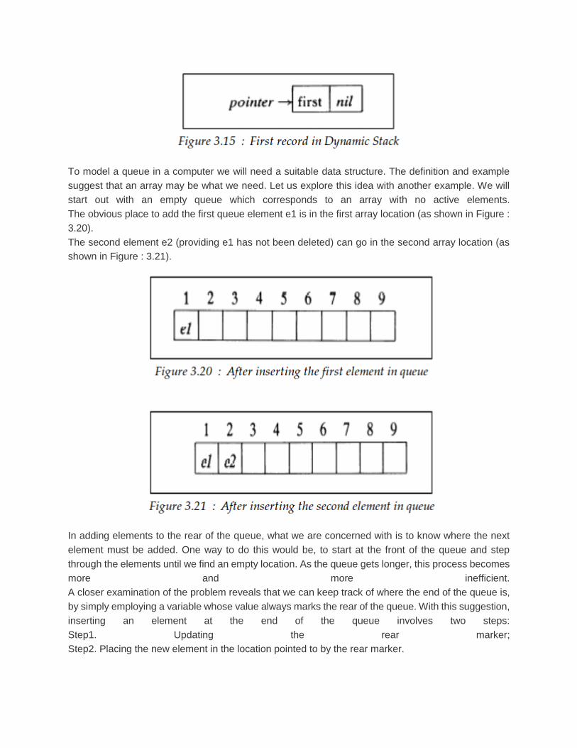
To model a queue in a computer we will need a suitable data structure. The definition and example

suggest that an array may be what we need. Let us explore this idea with another example. We will

start out with an empty queue which corresponds to an array with no active elements.

The obvious place to add the first queue element e1 is in the first array location (as shown in Figure :

3.20).

The second element e2 (providing e1 has not been deleted) can go in the second array location (as

shown in Figure : 3.21).

In adding elements to the rear of the queue, what we are concerned with is to know where the next

element must be added. One way to do this would be, to start at the front of the queue and step

through the elements until we find an empty location. As the queue gets longer, this process becomes

more and more inefficient.

A closer examination of the problem reveals that we can keep track of where the end of the queue is,

by simply employing a variable whose value always marks the rear of the queue. With this suggestion,

inserting an element at the end of the queue involves two steps:

Step1. Updating the rear marker;

Step2. Placing the new element in the location pointed to by the rear marker.

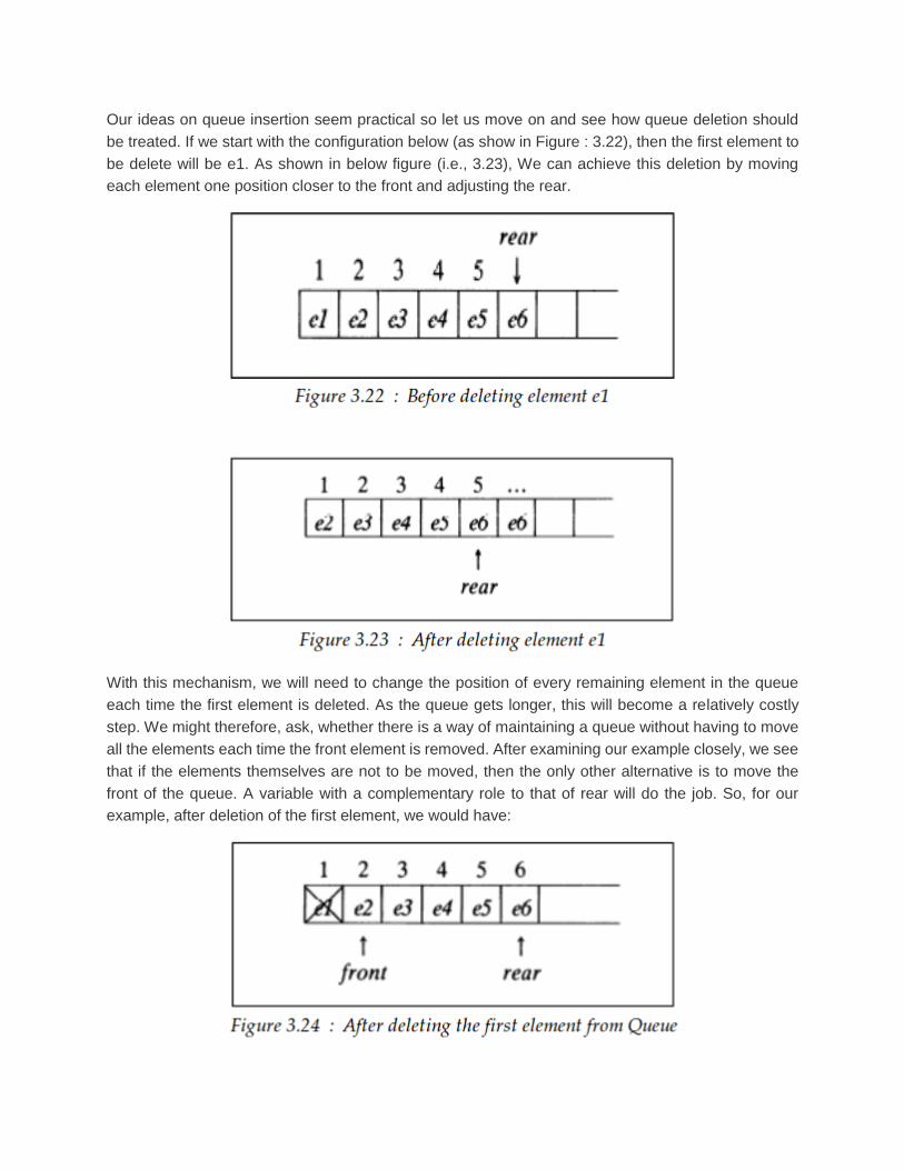
Our ideas on queue insertion seem practical so let us move on and see how queue deletion should

be treated. If we start with the configuration below (as show in Figure : 3.22), then the first element to

be delete will be e1. As shown in below figure (i.e., 3.23), We can achieve this deletion by moving

each element one position closer to the front and adjusting the rear.

With this mechanism, we will need to change the position of every remaining element in the queue

each time the first element is deleted. As the queue gets longer, this will become a relatively costly

step. We might therefore, ask, whether there is a way of maintaining a queue without having to move

all the elements each time the front element is removed. After examining our example closely, we see

that if the elements themselves are not to be moved, then the only other alternative is to move the

front of the queue. A variable with a complementary role to that of rear will do the job. So, for our

example, after deletion of the first element, we would have:

We now have mechanisms for queue insertion and deletion. As more insertions and deletions are

made, the current queue entries are going to be displaced further and further to the right(towards the

high suffix end) of the array. To give an example, initially we might have the following queue

parameters:

front = 1, rear = 25, queue length = 25 {queue length = rear - front +1}

And some considerable time later after a number of insertions and deletions:

front = 87, rear = 102, queue length = 16

Maintenance of queue in an array

These examples imply that over a long period of time, we may face a very high storage cost. This

excessive use of storage is obviously going to make our current proposal unacceptable for practical

use.

Ideally it would be desirable to have to commit only an amount of storage, equal to the maximum

anticipated queue length. This goal seems reasonable since in many applications, because of the way

insertions and deletions compete; the queue length is relatively stable.

From our earlier example it is clear that a queue can be maintained within an array greater than or

equal to its maximum length by shifting the elements as we had originally proposed. The question that

remains is, can we do it without having to move all the elements after each deletion? One idea might

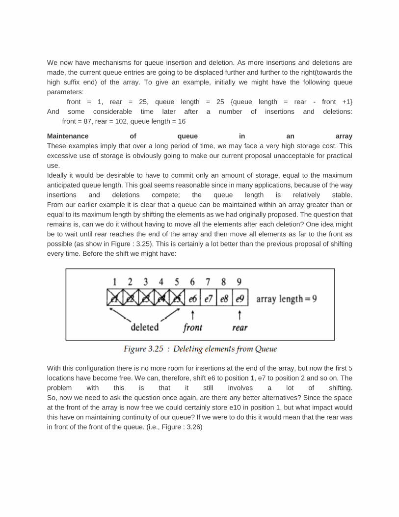
be to wait until rear reaches the end of the array and then move all elements as far to the front as

possible (as show in Figure : 3.25). This is certainly a lot better than the previous proposal of shifting

every time. Before the shift we might have:

With this configuration there is no more room for insertions at the end of the array, but now the first 5

locations have become free. We can, therefore, shift e6 to position 1, e7 to position 2 and so on. The

problem with this is that it still involves a lot of shifting.

So, now we need to ask the question once again, are there any better alternatives? Since the space

at the front of the array is now free we could certainly store e10 in position 1, but what impact would

this have on maintaining continuity of our queue? If we were to do this it would mean that the rear was

in front of the front of the queue. (i.e., Figure : 3.26)

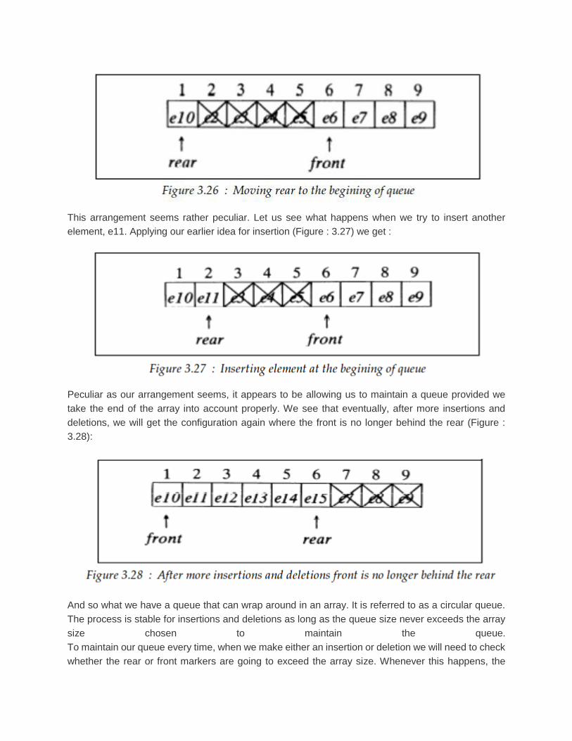
This arrangement seems rather peculiar. Let us see what happens when we try to insert another

element, e11. Applying our earlier idea for insertion (Figure : 3.27) we get :

Peculiar as our arrangement seems, it appears to be allowing us to maintain a queue provided we

take the end of the array into account properly. We see that eventually, after more insertions and

deletions, we will get the configuration again where the front is no longer behind the rear (Figure :

3.28):

And so what we have a queue that can wrap around in an array. It is referred to as a circular queue.

The process is stable for insertions and deletions as long as the queue size never exceeds the array

size chosen to maintain the queue.

To maintain our queue every time, when we make either an insertion or deletion we will need to check

whether the rear or front markers are going to exceed the array size. Whenever this happens, the

corresponding marker will need to be reset to 1.Having worked out our basic mechanism for

maintaining a queue in an array, our next task is to take a closer look at the design of the insertion

and deletion algorithms. Examining our queue data structure carefully we see that a number of

conditions can apply when we want to make the next insertion:

1. The queue can be empty

2. The queue can be already full.

3. The end of the array has been reached prior to the insertion.

4. None of the above conditions apply (the most likely case).

We might anticipate that at least some of these cases will appear, other than direct insertion in the

next location. An important case that we must consider is when an attempt is made to insert into a full

queue. From our previous examples, it would seem that the easiest way to do this would be to check

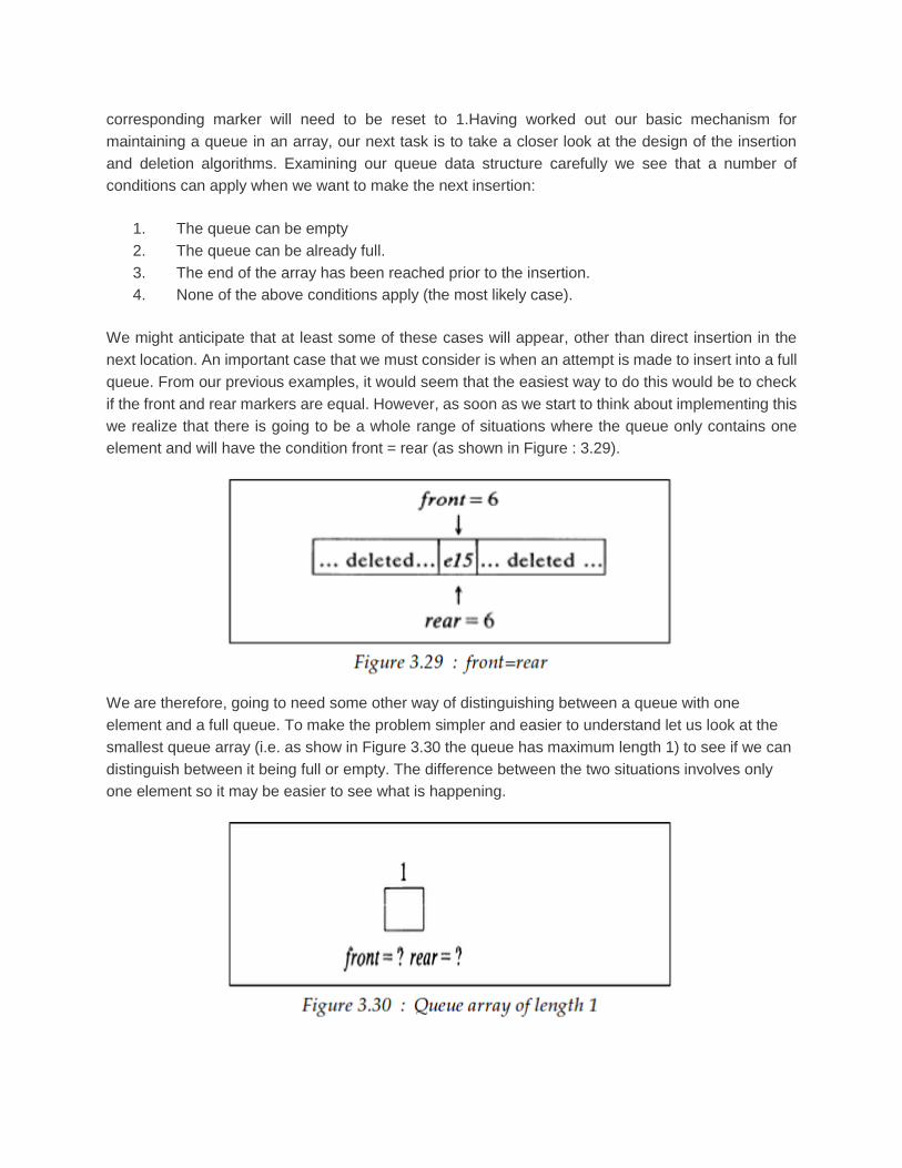
if the front and rear markers are equal. However, as soon as we start to think about implementing this

we realize that there is going to be a whole range of situations where the queue only contains one

element and will have the condition front = rear (as shown in Figure : 3.29).

We are therefore, going to need some other way of distinguishing between a queue with one

element and a full queue. To make the problem simpler and easier to understand let us look at the

smallest queue array (i.e. as show in Figure 3.30 the queue has maximum length 1) to see if we can

distinguish between it being full or empty. The difference between the two situations involves only

one element so it may be easier to see what is happening.

Normally when an insertion is made, rear is increased by one and the element is placed in the queue.

If we were to apply this rule in the present case rear would need to have been initially set to zero.

There is then the question of what to do about the front initially and after deletion. Only two possibilities

exist for our one element array. The marker can only be either 0 or 1 before the insertion. If we choose

front = 1 initially (as shown in Figure : 3.31), we have:

Let us see what appens now, when we delete an element. This involves increasing front by one but

since it takes us beyond the end of the array, it must be reset to the start of the array. There is a

problem here because the start and end of the array are at the same position and so once again, on

deletion in this way, we would end up with,

This contradicts the earlier situation. Because of this problem let us look at the other alternative

starting out with front = 0.

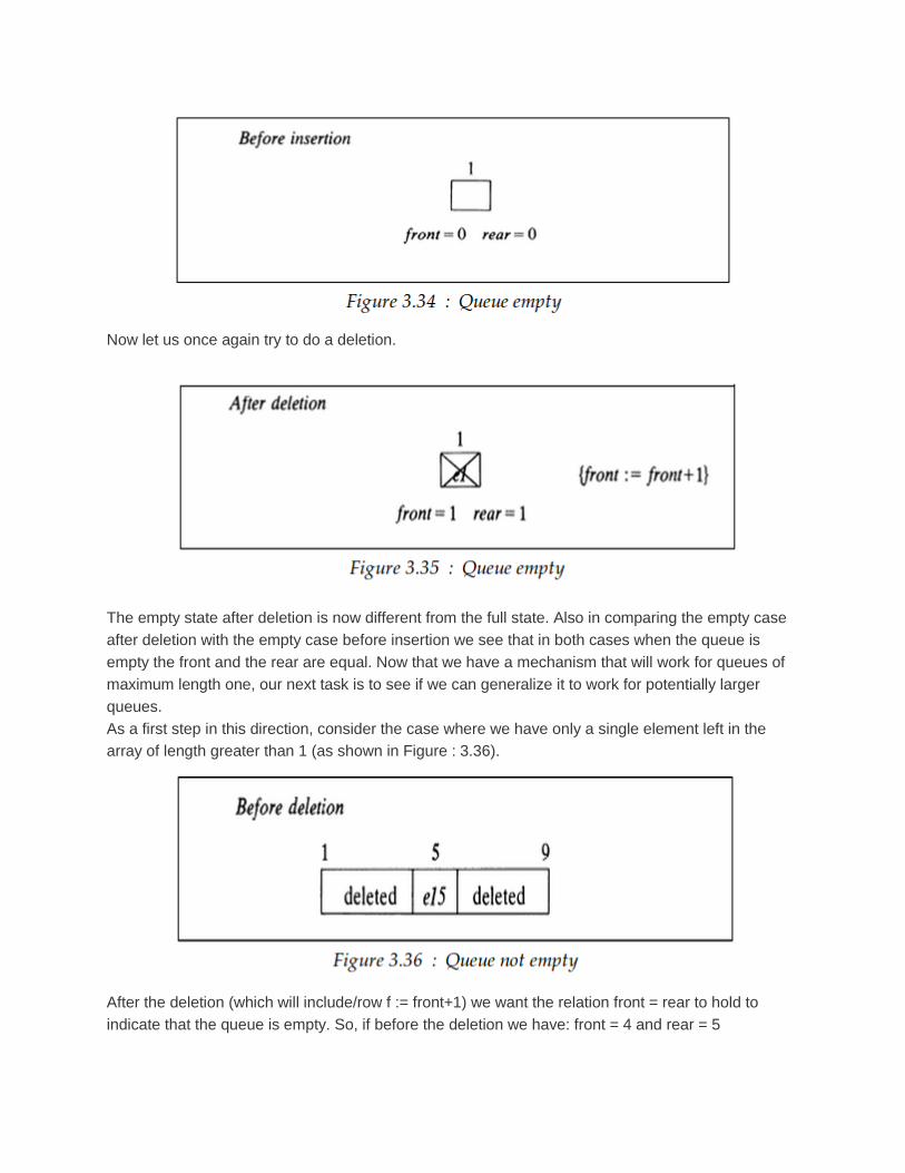
Now let us once again try to do a deletion.

The empty state after deletion is now different from the full state. Also in comparing the empty case

after deletion with the empty case before insertion we see that in both cases when the queue is

empty the front and the rear are equal. Now that we have a mechanism that will work for queues of

maximum length one, our next task is to see if we can generalize it to work for potentially larger

queues.

As a first step in this direction, consider the case where we have only a single element left in the

array of length greater than 1 (as shown in Figure : 3.36).

After the deletion (which will include/row f := front+1) we want the relation front = rear to hold to

indicate that the queue is empty. So, if before the deletion we have: front = 4 and rear = 5

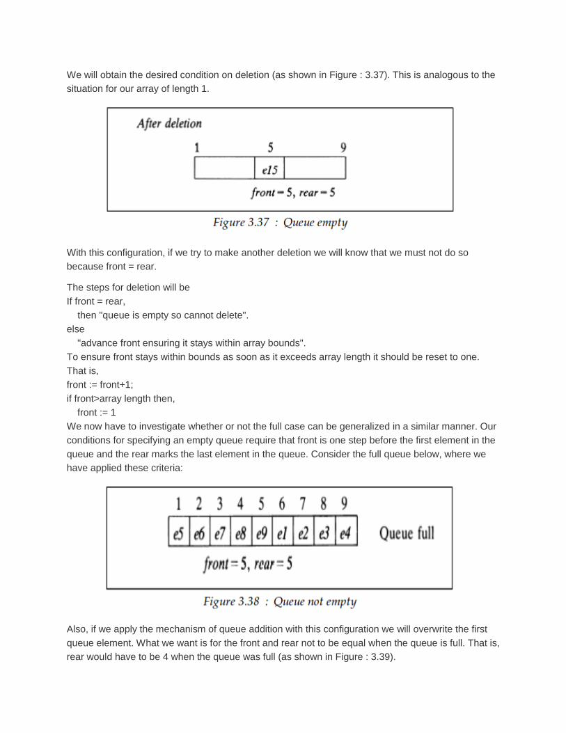
We will obtain the desired condition on deletion (as shown in Figure : 3.37). This is analogous to the

situation for our array of length 1.

With this configuration, if we try to make another deletion we will know that we must not do so

because front = rear.

The steps for deletion will be

If front = rear,

then "queue is empty so cannot delete".

else

"advance front ensuring it stays within array bounds".

To ensure front stays within bounds as soon as it exceeds array length it should be reset to one.

That is,

front := front+1;

if front>array length then,

front := 1

We now have to investigate whether or not the full case can be generalized in a similar manner. Our

conditions for specifying an empty queue require that front is one step before the first element in the

queue and the rear marks the last element in the queue. Consider the full queue below, where we

have applied these criteria:

Also, if we apply the mechanism of queue addition with this configuration we will overwrite the first

queue element. What we want is for the front and rear not to be equal when the queue is full. That is,

rear would have to be 4 when the queue was full (as shown in Figure : 3.39).

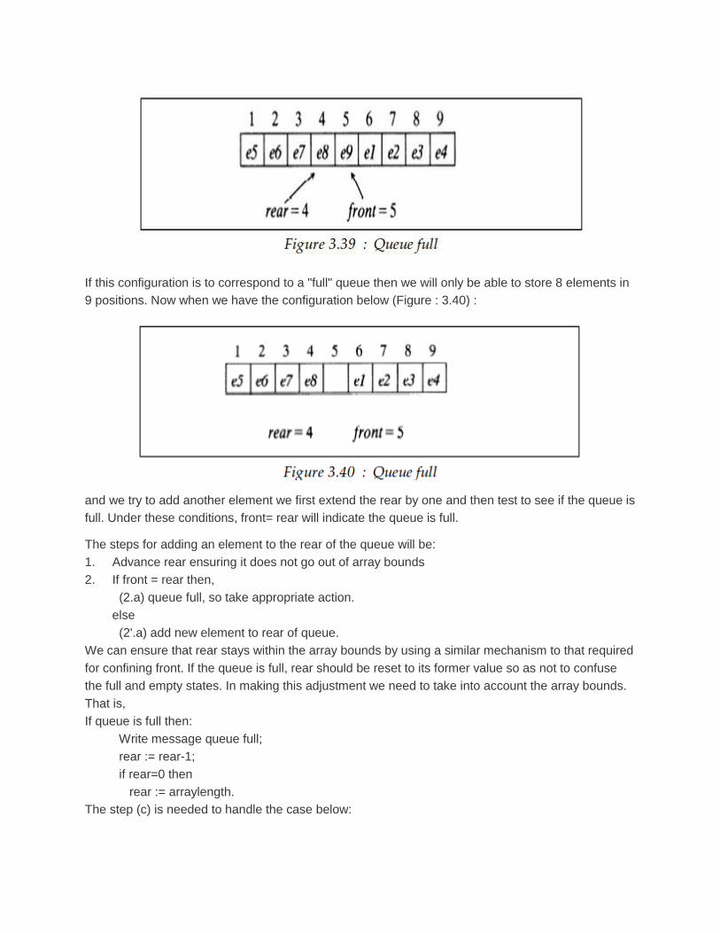
If this configuration is to correspond to a "full" queue then we will only be able to store 8 elements in

9 positions. Now when we have the configuration below (Figure : 3.40) :

and we try to add another element we first extend the rear by one and then test to see if the queue is

full. Under these conditions, front= rear will indicate the queue is full.

The steps for adding an element to the rear of the queue will be:

1. Advance rear ensuring it does not go out of array bounds

2. If front = rear then,

(2.a) queue full, so take appropriate action.

else

(2'.a) add new element to rear of queue.

We can ensure that rear stays within the array bounds by using a similar mechanism to that required

for confining front. If the queue is full, rear should be reset to its former value so as not to confuse

the full and empty states. In making this adjustment we need to take into account the array bounds.

That is,

If queue is full then:

Write message queue full;

rear := rear-1;

if rear=0 then

rear := arraylength.

The step (c) is needed to handle the case below:

The descriptions for queue insertion and deletion will now be outlined.It will be assumed that front

and rear are both one when the queue is initially empty.

Algorithm description

1. Queue insertion

1. Establish the queue, data for insertion, array length, front, and rear.

2. Advance the rear according to mechanism for keeping it within array bounds.

3. If front not equal to rear then,

(3.a) insert data at next available position in queue.

else

(3.a') queue is full so write out full signal.

(3.b) restore rear marker to its previous value taking into account array bounds.

4. Return updated queue and its adjusted rear pointer.

2. Queue deletion

1. Establish queue, array length, front and rear markers.

2. If front is not equal to rear then,

(2.a) advance front according to mechanism for keeping it within array bounds,

remove element from front of queue,

else

(2.a') queue empty so write out empty message.

3. Return updated queue, the element off the front of the queue and adjust the front

marker.

Performance Analysis

Queue operations involve essentially one compound step and so their time complexity is of little

interest.