Screening Data

Many of my students have gotten “spoiled” because I nearly always provide them with clean data. By “clean data” I mean data which has already been screened to remove out-of range values, transformed to meet the assumptions of the analysis to be done, and otherwise made ready to use. Sometimes these spoiled students have quite a shock when they start working with dirty data sets, like those they are likely to encounter with their thesis, dissertation, or other research projects. Cleaning up a data file is like household cleaning jobs—it can be tedious, and few people really enjoy doing it, but it is vitally important to do. If you don’t clean your dishes, scrub the toilet, and wash your clothes, you get sick. If you don’t clean up your research data file, your data analysis will produce sick (schizophrenic) results. You may be able to afford to pay someone to clean your household. Paying someone to clean up your data file can be more expensive (once you know how to do it you may be willing to do it for others, if compensated well—I charge $250 an hour, the same price I charge for programming, interpreting, and writing).

Missing DataWith some sorts of research it is not unusual to have cases for which there are missing data

for some but not all variables. There may or there may not be a pattern to the missing data. The missing data may be classified as MCAR, MAR, or MNAR.Missing Not at Random (MNAR)

Some cases are missing scores on our variable of interest, Y. Suppose that Y is the salary of faculty members. Missingness on Y is related to the actual value of Y. Of course, we do not know that, since we do not know the values of Y for cases with missing

data. For example, faculty with higher salaries may be more reluctant to provide their income. If we estimate mean faculty salary with the data we do have on hand it will be a biased

estimate. There is some mechanism which is causing missingness, but we do not know what it is.

Missing At Random (MAR) Missingness on Y is not related to the true value of Y itself or is related to Y only through its

relationship with another variable or set of variables, and we have scores on that other variable or variables for all cases.

For example, suppose that the higher a professor’s academic rank the less likely e is to provide e’s salary. Faculty with higher ranks have higher salaries. We know the academic rank of each respondent.

We shall assume that within each rank whether Y is missing or not is random – of course, this may not be true, that is, within each rank the missingness of Y may be related to the true value of Y.

Again, if we use these data to estimate mean faculty salary, the estimate will be biased. However, within conditional distributions the estimates will be unbiased – that is, we can

estimate without bias the mean salary of lecturers, assistant professors, associate professors, and full professors.

Copyright 2016, Karl L. Wuensch - All rights reserved.Screen.docx

We might get an unbiased estimate of the overall mean by calculating a weighted mean of

the conditional means -- GM=ΣpiM i , where GM is the estimated grand mean, pi is, for each

rank, the proportion of faculty at that rank, and Mi is the estimated mean for each rank.

Missing Completely at Random (MCAR) There is no variable, observed or not, that is related to the missingness of Y. This is probably

never absolutely true, but we can pretend that it is.

Finding Patterns of Missing DataThe MVA module mentioned in Tabachnik and Fidell is an add-on that is sometimes included

with SPSS, sometimes not. Curiously, the version of SPSS (20) distributed to faculty to use on campus at ECU does not contain the MVA and multiple imputation modules, but that distributed for off campus use does. You can, however, obtain the same t tests that are produced by MVA without having that module. Suppose that the variable of interest is income and you are concerned only with how missingness on income is related with scores on the other variables. Create a missingness dummy variable (0 = not missing the income score, 1 = missing the income score). Now use t tests (or Pearson r ) to see if missingness on income is related to the other variables (MAR).

Dealing with the Problem of Missing DataDeletion of Cases. Delete from the data analyzed any case that is missing data on any of the

variables used in the analysis. If there are not a lot of cases with missing data and you are convinced that the missing data are MCAR, then this is an easy and adequate solution. Estimates will not be biased. Of course, the reduction of sample size results in a loss of power and increased error in estimation (wider confidence intervals).

Deletion of Variables. Delete any variable that is missing data on many cases. This is most helpful when you have another variable that is well related to the troublesome variable and on which there are not many missing values.

Mean Substitution. For each missing data point, impute the mean on that variable. “Imputation” is the substitution of an estimated value in this case a mean) for the missing value. If the cases are divided into groups, substitute the mean of the group in which the case belongs. While this does not alter the overall or group means, it does reduce the overall or group standard deviations, which is undesirable.

Missingness Dummy Variable. Maybe the respondents are telling you something important by not answering one of the questions. Set up a dummy variable with value 0 for those who answered the question and value 1 for those who did not. Use this dummy variable as one of the predictors of the outcome variable. You may also try using both a missingness dummy variable and the original variable with means imputed for missing values.

Regression. Develop a multiple regression to predict values on the variable which has missing cases from the other variables. Use the resulting regression line to predict the missing values. Regression towards the mean will reduce the variability of the data, especially if the predicted variable is not well predicted from the other variables.

Multiple Imputation. A random sample (with replacement) from the data set is used to develop the model for predicting missing values. Those predictions are imputed. A second random sample is used to develop a second model and its predictions are imputed. This may be done three or more times. Now you have three or more data sets which differ with respect to the imputed values. You conduct your analysis on each of these data sets and then average the results across data sets. Later we shall study how to use SAS or SPSS for multiple imputation.

2

Pairwise Correlation Matrix. For the variables of interest, compute a correlation matrix that uses all available cases for each correlation. With missing data it will not be true that all of the correlations will be computed on the same set of cases, and some of the correlations may be based on many more cases than are others. After obtaining this correlation matrix, use it as input to the procedure that conducts your analysis of choice. This procedure can produce very strange results.

Can We Get Unbiased Estimates? Maybe. If the data are MCAR, even simple deletion of cases with missing data will allow unbiased

estimates. If the data are MAR the more sophisticated methods can provide unbiased estimates. If the data are MNAR then unbiased estimates are not possible, but modern methods may

allow one to reduce the bias in estimation.

Missing Item Data Within a Unidimensional ScaleSuppose that you have a twenty item scale that you trust is unidimensional. You have done

item analysis and factor analysis that supports your contention that each item (some of them first having been reflected) measures the same construct (latent variable). Some of your subjects have failed to answer one or more of the items on your scale. What to do?

A relatively simple solution is to compute, for each subject, the mean of that subject’s scores on the items he or she did answer on that scale. If all of the items are measuring the same construct (with the same metric), that should give you a decent estimate of the subject’s standing on that construct. Please note that this is not what is commonly referred to as “mean substitution.” With “mean substitution,” one substitutes for the missing item score the mean score from other subjects on that item. The procedure described here is known as person-mean imputation.

Essentially what you are doing here is estimating the subject’s missing score from his or her scores on the remaining items on the scale. This technique is sometimes called “Person Mean Imputation.” At the time I am writing this, one of our brilliant graduate students, Sydney Siver, is conducting Monte Carlo research comparing Person Mean Imputation with more sophisticated methods of imputation. I can hardly wait to see her results.

Suppose you have a twenty item, unidimensional scale that measures misanthropy. Some respondents have failed to answer some of the questions. What should you do? The first thing you should do is to see how many missing scores there were on each item. If an item has a large proportion of missing scores, you need to try to figure out why. You may need to remove that item from the scale, at least for the current sample.

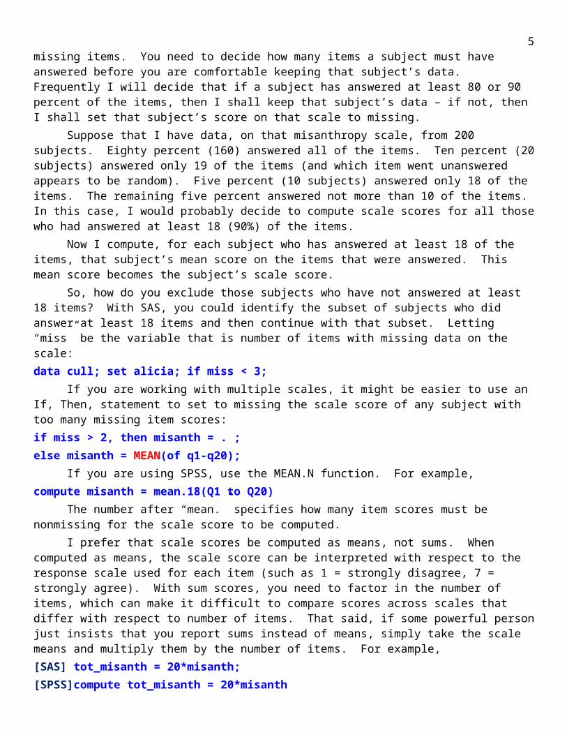
Next you need to determine, for each subject, how many of the items were missing. If you are using SAS or SPSS, see my lesson on the use of the SUM, MEAN, and NMISS functions. Look at the distribution of number of missing items. You need to decide how many items a subject must have answered before you are comfortable keeping that subject’s data. Frequently I will decide that if a subject has answered at least 80 or 90 percent of the items, then I shall keep that subject’s data – if not, then I shall set that subject’s score on that scale to missing.

Suppose that I have data, on that misanthropy scale, from 200 subjects. Eighty percent (160) answered all of the items. Ten percent (20 subjects) answered only 19 of the items (and which item went unanswered appears to be random). Five percent (10 subjects) answered only 18 of the items. The remaining five percent answered not more than 10 of the items. In this case, I would probably decide to compute scale scores for all those who had answered at least 18 (90%) of the items.

Now I compute, for each subject who has answered at least 18 of the items, that subject’s mean score on the items that were answered. This mean score becomes the subject’s scale score.

3

So, how do you exclude those subjects who have not answered at least 18 items? With SAS, you could identify the subset of subjects who did answer at least 18 items and then continue with that subset. Letting “miss” be the variable that is number of items with missing data on the scale:data cull; set alicia; if miss < 3;

If you are working with multiple scales, it might be easier to use an If, Then, statement to set to missing the scale score of any subject with too many missing item scores:if miss > 2, then misanth = . ;else misanth = MEAN(of q1-q20);

If you are using SPSS, use the MEAN.N function. For example, compute misanth = mean.18(Q1 to Q20)

The number after “mean.” specifies how many item scores must be nonmissing for the scale score to be computed.

I prefer that scale scores be computed as means, not sums. When computed as means, the scale score can be interpreted with respect to the response scale used for each item (such as 1 = strongly disagree, 7 = strongly agree). With sum scores, you need to factor in the number of items, which can make it difficult to compare scores across scales that differ with respect to number of items. That said, if some powerful person just insists that you report sums instead of means, simply take the scale means and multiply them by the number of items. For example,[SAS] tot_misanth = 20*misanth;[SPSS]compute tot_misanth = 20*misanth

If you decide to use the SUM function in SAS or SPSS, be very careful, it will treat missing values as zeros. See SUM, MEAN, and NMISS .

Once a friend suggested that using means across items rather than sums across items would produce a restriction of range and accordingly lower the magnitude of the associations between the scale scores and other variables. This absolutely false. The relationship between X and Y is absolutely unaltered by replacing X and/or Y with any linear transformation of X and/or Y

OutliersUnivariate outliers are scores on a single variable that are very unusual – that is, scores

which are far away from the mean on that variable. My preferred method of detecting univariate outliers is the box and whiskers plot.

Multivariate outliers are cases where there is an unusual combination of values on two or more of the variables. Suppose one of our variables is number of years since a faculty member received her Ph.D. and another is number of publications. Three years is not a very unusual value on the one variable, and thirty publications may not be a very unusual value on the other variable, but a case with values of three years and thirty publications is probably a rather unusual combination of values.

The Mahalanobis distance or the closely related leverage can be employed to detect multivariate outliers. Suppose we have three variables (X, Y, and Z). Imagine a three dimensional plot where X is plotted on the horizontal dimension, Y on the vertical, and Z on the depth. The plotted scores are represented as points in three dimensional space. Now add a central reference point which has as its values the mean on X, the mean on Y and the mean on Z. This is the centroid. The Mahalanobis distance (MD) is a measure of the geometric distance between the point representing

any one of the cases and this centroid. Leverage is

MDN−1

+ 1N . You should investigate any case

where the leverage exceeds 2p/n, where p is the number of variables and n is the number of cases.

4

When there are only a few multivariate outliers, examine each individually to determine how they differ from the centroid. When there are many outliers you may want to describe how the outliers as a group differ from the centroid – just compare the means of the outliers with the means of the total data set. If there are many variables you may create an outlier dummy variable (0 = not an outlier, 1 = is an outlier) and predict that dummy variable from the other variables. The other variables which are well related to that dummy variable are those variables on which the outliers as a group differ greatly from the centroid.

Regression diagnostics should be employed to detect outliers, poorly fitting cases, and cases which have unusually large influence on the analysis. Leverage is used to identify cases which have unusual values on the predictor variables. Standardized residuals are used to identify cases which do not fit well with the regression solution. Cook’s D and several other statistics can be used to determine which cases have unusually large influence on the regression solution. See my introduction to the topic of regression diagnostics here.

Dealing with outliers. There are several ways to deal with outliers, including:

Investigation. Outlying observations may simply be bad data. There are many ways bad data can get into a data file. They may result from a typo. They may result from the use of a numeric missing value code that was not identified as such to the statistical software. The subject may have been distracted when being measured on a reaction time variable. While answering survey items the respondent may have unknowingly skipped question 13 and then put the response for question 14 in the space on the answer sheet for question 13 (and likewise misplaced the answers for all subsequent questions). When the survey questions shifted from five response options to four response options the respondent may have continued to code the last response option as E rather than D. You should investigate outliers (and out-of-range values, which may or may not be outliers) and try to determine whether the data are good or not and if not what the correct score is. At the very least you should go back to the raw data and verify that the scores were correctly entered into the data file. Do be sure that both your raw data and your data file have for each case a unique ID number so that you can locate in the raw data the case that is problematic.

Set the Outlier to Missing. If you decide that the score is bad and you decide that you cannot with confidence estimate what it should have been, change the bad score to a missing value code.

Delete the Case. If a case has so many outliers that you are convinced that the respondent was not even reading the questions before answering them (this happens more often that most researchers realize), you may decide to delete all data from the troublesome case. Sometimes I add to my survey items like “I frequently visit planets outside of this solar system” and “I make all my own clothes” just to trap those who are not reading the items. You may also delete a case when your investigation reveals that the subject is not part of the population to which you wish to generalize your results.

Delete the Variable. If one variable has very many outliers that cannot be resolved, you may elect to discard that variable from the analysis.

Transform the Variable. If you are convinced that the outlier is a valid score, but concerned that it is making the distribution badly skewed, you may chose to apply a skewness-reducing transformation.

Change the Score. You may decide to retain the score but change it so it is closer to the mean – for example, if the score is in the upper tail, changing it to one point more than the next highest score.

Assumptions of the Analysis

5

You should check your data to see if it about what you would expect if the assumptions in your analysis were correct. With many analyses these assumptions are normality and homoscedasticity.

Normality. Look at plots and values of skewness and kurtosis. Do not pay much attention to tests of the hypothesis that the population is normally distributed or that skewness or kurtosis is zero in the population – if you have a large sample these tests may be significant when the deviation from normality is trivial and of no concern, and if you have a small sample these tests may not be significant when you have a big problem. If you have a problem you may need to transform the variable or change the sort of analysis you are going to conduct. See Checking Data For Compliance with A Normality Assumption.

Homogeneity of Variance. Could these sample data have come from populations where the group variances were all identical? If the ratio of the largest group variance to the smallest group variance is large, be concerned. There is much difference of opinion regarding how high that ratio must be before you have a problem. If you have a problem you may need to transform the variable or change the sort of analysis you are going to conduct.

Homoscedasticity. This the homogeneity of variance assumption in correlation/regression analysis. Careful inspection of the residuals should reveal any problem with heteroscedasticity. Inspection of the residuals can also reveal problems with the normality assumption and with curvilinear effects that you had not anticipated. See Bivariate Linear Regression and Residual Plots. If you have a problem you may need to transform the variable or change the sort of analysis you are going to conduct.

Homogeneity of Variance/Covariance Matrices. Box’s M is used to test this assumption made when conducting a MANOVA and some other analyses. M is very powerful, so we generally do not worry unless it is significant beyond .001.

Sphericity. This assumption is made with univariate-approach correlated samples ANOVA. Suppose that we computed difference scores (like those we used in the correlated t-test) for Level 1 vs. Level 2, Level 1 vs. Level 3, Level 1 vs. Level 4, and every other possible pair of levels of the repeated factor. The sphericity assumption is that the standard deviation of each of these sets of difference scores (1 vs 2, 1 vs 3, etc.) is a constant in the population. Mauchley’s test is used to evaluate this assumption. If it is violated there you can stick with the univariate approach but reduce the df, or you can switch to the multivariate-approach which does not require this assumption.

Homogeneity of Regression. This assumption is made when conducting an ANCOV. It can be tested by testing the interaction between groups and the covariate.

Linear Relationships. The analyses most commonly employed by psychologists are intended to detect linear relationships. If the relationships are nonlinear then you need to take that into account. It is always a good idea to look at scatter plots showing the nature of the relationships between your variables. See Importance of Looking at a Scatterplot Before You Analyze Your Data and Curvilinear Bivariate Regression.

MulticollinearityMulticollinearity exits when one of your predictor variables can be nearly perfectly predicted by

one of the other predictor variables or a linear combination of the other predictor variables. This is a problem because it makes the regression coefficients unstable in the sense that if you were to draw several random samples from the same population and conduct your analysis on each you would find that the regression coefficients vary greatly from sample to sample. If there is perfect relationship between one of your predictors and a linear combination of the others then the intercorrelation matrix

6

is singular. Many analyses require that this matrix be inverted, but a singular matrix cannot be inverted, so the program crashes. Here is a simple example of how you could get a singular intercorrelation matrix: You want to predict college GPA from high school grades, verbal SAT, math SAT, and total SAT. Oops, each of the SAT variables can be perfectly predicted from the other two.

To see if multicollinearity exists in your data, compute for each predictor variable the R2 for predicting it from the others. If that R2 is very high (.9 or more), you have a problem. Statistical programs make it easy to get the tolerance (1 that R2 ). Low values of tolerance signal trouble.

Another problem with predictors that are well correlated with one another is that the analysis will show that they have little unique relationship with the outcome variable (since they are redundant with each other). This is a problem because many psychologists do not understand redundancy and then conclude that none of those redundant variables are related to the outcome variable.

There are several ways to deal with multicollinearity:

Drop a Predictor. The usual way of dealing with the multicollinearity problem is to drop one or more of the predictors from the analysis including:

Combine Predictors. Combine into a composite variable the redundant predictor variables.

Principal Components Analysis. Conduct a principal components analysis on the data and output the orthogonal component scores, for which there will be no multicollinearity. You can then conduct your primary analysis on the component scores and transform the results back into the original variables.

SASDownload the Screen.dat data file from my StatData page and the program Screen.sas from

my SAS-Programs page. Edit the infile statement so it correctly points to the place where you deposited Screen.dat and then run the program. This program illustrates basic data screening techniques. The data file is from a thesis long ago. Do look at the questionnaire while completing this lesson. I have put numbered comment lines in the SAS program (comment lines start with an asterisk) corresponding to the numbered paragraphs below.****************************************************************************;data delmel; infile 'C:\Users\Vati\Documents\StatData\Screen.dat'; * 1: ALWAYS include an identification number;input ID 1-3 @5 (Q1-Q138) (1.);label Q1='Sex' Q3 = 'Age' Q5='CitySize' Q6='CityCountry' Q67='SibsMental';

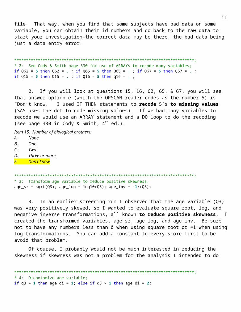
1. One really should give each subject (or participant, event, case, observation) an identification number and enter that number in the data file. That way, when you find that some subjects have bad data on some variable, you can obtain their id numbers and go back to the raw data to start your investigation—the correct data may be there, the bad data being just a data entry error.

****************************************************************************;* 2: See Cody & Smith page 330 for use of ARRAYs to recode many variables;if Q62 = 5 then Q62 = . ; if Q65 = 5 then Q65 = . ; if Q67 = 5 then Q67 = . ;if Q15 = 5 then Q15 = . ; if Q16 = 5 then q16 = . ;

7

2. If you will look at questions 15, 16, 62, 65, & 67, you will see that answer option e (which the OPSCAN reader codes as the number 5) is “Don’t know.” I used IF THEN statements to recode 5’s to missing values (SAS uses the dot to code missing values). If we had many variables to recode we would use an ARRAY statement and a DO loop to do the recoding (see page 330 in Cody & Smith, 4th ed.).Item 15. Number of biological brothers:A. NoneB. OneC. TwoD. Three or moreE. Don’t know

****************************************************************************;* 3: Transform age variable to reduce positive skewness;age_sr = sqrt(Q3); age_log = log10(Q3); age_inv = -1/(Q3);

3. In an earlier screening run I observed that the age variable (Q3) was very positively skewed, so I wanted to evaluate square root, log, and negative inverse transformations, all known to reduce positive skewness. I created the transformed variables, age_sr, age_log, and age_inv. Be sure not to have any numbers less than 0 when using square root or =1 when using log transformations. You can add a constant to every score first to be avoid that problem.

Of course, I probably would not be much interested in reducing the skewness if skewness was not a problem for the analysis I intended to do.

****************************************************************************;* 4: Dichotomize age variable;if q3 = 1 then age_di = 1; else if q3 > 1 then age_di = 2;

4. Sometimes you just can’t get rid of that skewness. One might resort to nonparametric procedures (use a rank transformation) or resampling statistics, or one might just dichotomize the variable, as I have done here. Even after dichotomizing a predictor you may have trouble – if almost all of the scores fall into one group and very few into the other then you will have very low power for detecting the effect of that predictor. Dichotomizing a badly skewed variable has been common practice among researchers, but statisticans (if they are not badly out-of-date with the literature) now know that this is poor practice (Irwin & McClelland, 2003.

****************************************************************************;* 5: Create siblings variable;SIBS = Q15 + Q16;

5. I summed the brothers and sisters variables to create the siblings variable.

****************************************************************************;* 6: Transform sibs variable to reduce positive skewness;sibs_sr = sqrt(sibs); sibs_log = log10(sibs); sibs_in = -1/sibs;

6. SIBS is positively skewed, so I tried transformations on it too.

8

****************************************************************************;* 7: Create mental variable and dummy variable for missing data on Mental;MENTAL = Q62 + Q65 + Q67;MentalMiss = 0; If Mental = . then MentalMiss = 1;

7. I created the MENTAL variable, on which low scores mean the participant thinks that e’s close relatives are mentally unstable. I also created a dummy variable to indicate whether or not a case was missing data on the mental variable. For items 65 and 67, substitute “mother’s” or “brothers and/or sisters” for “father’s.”Item 62. My father’s mental health is (was) generally:A. Very poorB. FairC. GoodD. ExcellentE. Don’t know

****************************************************************************;* 8: Transform and reflect/transform Mental to reduce negative skewness;Mental2 = Mental*Mental;Mental3 = Mental**3;Ment_exp = EXP(Mental);R_Ment = 13 - Mental; R_Ment_sr = sqrt(R_Ment); R_Ment_log = log10(R_Ment);

8. The mental variable is negatively skewed. My program evaluates the effect of several different transformations that should reduce negative skewness. One can reduce negative skewness by squaring the scores or raising them to an even higher power. Be sure not to have any negative scores before such a transformation, adding a constant first, if necessary. Another transformation

which might be helpful is exponentiation. Exponentiated Y is Y exp=e

Y

, where e is the base of the natural logarithm, 2.718...... You may also need to reduce the values of the scores by dividing by a constant, to avoid producing transformed scores so large that they exceed the ability of your computer to record them. If your highest raw score were a 10, your highest transformed score would be a 22,026. A 20 would transform to 485,165,195. If you have ever wondered what is "natural" about the natural log, you can find an answer of sorts at http://www.math.toronto.edu/mathnet/answers/answers_13.html.

Another approach is first to reflect the variable (subtract it from a number one greater than its maximum value, making it positively skewed) and then apply transformations which reduce positive skewness. When interpreting statistics done on the reflected variable, we need to remember that after reflection it is high (rather than low) scores which indicate that the participant thinks e’s close relatives are mentally ill. A simple way to avoid such confusion is to rereflect the variable after transformation. For example, graduate student Megan Jones is using job satisfaction (JIG) as the criterion variable in a sequential multiple regression. It is badly negatively skewed, g2 = -1.309. Several transformations are tried. The transformation that works best is a log transformation of the reflected scores. For that log transformation g2 = -.191 and the maximum score is 1.43. The transformed scores are now subtracted from 1.5 to obtain a doubly reflected log transformation of the original scores with g2 = +.191. If we were to stick with the singly reflected transformation scores, we would need to remember that high scores now mean low job satisfaction. With the doubly reflected transformed scores high scores represent high job satisfaction, just as with the untransformed JIG scores.

9

****************************************************************************;* 9: Dichotomize Mental. BEWARE: SAS codes missing values with a negative number -- if you said 'If Mental LE 9 then Ment_di = 1' then observations with missing values would be recoded to 1;

9. I tried dichotomizing the mental variable too. Note that when doing this recoding I was careful not to tell SAS to recode all negative values. The internal code which SAS uses to stand for a missing value is a large negative number, so if you just tell it to recode all values below some stated value it will also recode all missing values on that variable. That could be a very serious error! We are supposed to be cleaning up these data, not putting in more garbage! Run the program If_Then.sas to illustrate the problem created if you forget that SAS represents missing values with extreme negative numbers.

****************************************************************************;* 10: Check for out of range values and missing data;title 'Check for out of range values and missing data'; run;proc means min max n nmiss; var q1-q10 q50-q70; run;

10. The first PROC statement simply checks for out-of-range values. Look at the output for Q9 and then look at question 9. There are only three response options for question nine, but we have a maximum score of 5 — that is, we have “out-of-range” data. Looks like at least one of our student participants wasn’t even able to maintain attention for nine items of the questionnaire!Item 9. Is your father living?A. YesB. NoC. Don’t know

Variable Label Minimum Maximum N N Miss

Q1Q2Q3Q4Q5Q6Q7Q8Q9Q10Q50Q59Q66Q67

SexAgeCitySizeCityCountrySibsMental

1.0000000

1.0000000

1.0000000

1.0000000

1.0000000

1.0000000

1.0000000

1.0000000

1.0000000

2.0000000

1.0000000

1.0000000

1.0000000

1.0000000

2.0000000

5.0000000

4.0000000

4.0000000

5.0000000

2.0000000

4.0000000

5.0000000

5.000000

210

210

210

210

210

210

210

210

210

210

210

210

209

198

0

0

0

0

0

0

0

0

0

0

0

0

1

12

10

Variable Label Minimum Maximum N N Miss

Q68Q69Q70

1.0000000

1.0000000

1.0000000

0

5.0000000

4.0000000

5.0000000

5.0000000

4.0000000

5.0000000

5.0000000

5.0000000

209

210

207

1

0

3

****************************************************************************;* 11: Check for skewness etc. Note use of -- list;title 'Check for skewness and kurtosis on original and transformed data'; run;proc means min max n nmiss skewness kurtosis; var Q3 age_sr -- Mental Mental2 -- R_Ment_log; run;

11. Here I check the skewness of variables in which I am interested, including transformations intended to normalize the data. Note the use of the “ ” to define a variable list: “A B” defines a list that includes all of the variables input or created from A through B. It works just like “TO” works in SPSS. Look at the output. Age (Q3) is very badly skewed. Although the transformations greatly reduce the skewness, even the strongest transformation didn’t reduce the skewness below 1, which is why I dichotomized the variable. The SIBS variable is not all that badly skewed, but the square root and log transformations improve it. Note that the inverse transformation is too strong, actually converting it to a negatively skewed variable. Notice that the absolute value of the skewness of the reflected MENTAL variable is the same as that of the original variable, but of opposite sign. The square root transformation normalizes it well.

Variable Label Minimum Maximum N N Miss

Skewness Kurtosis

Q3age_srage_logage_invage_diSIBS

Age 1.0000000

1.0000000

0

-1.0000000

1.0000000

2.0000000

4.0000000

2.0000000

0.6020600

-0.2500000

2.0000000

8.0000000

210

210

210

210

210

208

0

0

0

0

0

2

2.65956982.1555591

1.8256285

1.5221203

1.4026602

0.7963592

8.1218049

4.5322928

2.3728069

0.5809680

-0.0329493

0.4679821

11

Variable Label Minimum Maximum N N Miss

Skewness Kurtosis

sibs_srsibs_logsibs_inMENTALMental2Mental3Ment_expR_MentR_Ment_srR_Ment_log

1.4142136

0.3010300

-0.5000000

3.0000000

9.0000000

27.0000000

20.0855369

1.0000000

1.0000000

0

2.8284271

0.9030900

-0.1250000

12.0000000

144.0000000

1728.00

162754.79

10.0000000

3.1622777

1.0000000

208

208

208

193

193

193

193

193

193

193

2

2

2

17

17

17

17

17

17

17

0.3880711

-0.0302413-0.8737913

-0.9068181-0.3022089

0.04817890.9660522

0.90681810.2009510

-0.3123634

-0.0771341

-0.2210880

0.6219743

1.2237279

-0.5324565

-1.0829732

-0.7612228

1.2237279

-0.4982183

-1.0020210

****************************************************************************;* 12: Look at distributions in tables; run;title 'Frequency Distribution Tables';proc freq; tables q3 age_di sibs mental ment_di; run;

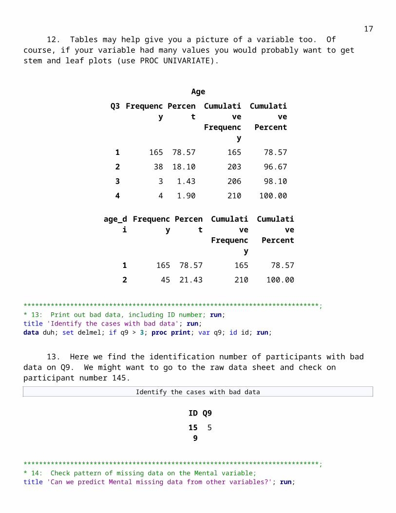
12. Tables may help give you a picture of a variable too. Of course, if your variable had many values you would probably want to get stem and leaf plots (use PROC UNIVARIATE).

AgeQ3 Frequenc

yPercent Cumulative

FrequencyCumulative

Percent1 165 78.57 165 78.57

2 38 18.10 203 96.67

3 3 1.43 206 98.10

4 4 1.90 210 100.00

age_di Frequency Percent Cumulative

Frequency

CumulativePercent

1 165 78.57 165 78.57

2 45 21.43 210 100.00

****************************************************************************;* 13: Print out bad data, including ID number; run;title 'Identify the cases with bad data'; run;data duh; set delmel; if q9 > 3; proc print; var q9; id id; run;

12

13. Here we find the identification number of participants with bad data on Q9. We might want to go to the raw data sheet and check on participant number 145.

Identify the cases with bad data

ID Q9159 5

****************************************************************************;* 14: Check pattern of missing data on the Mental variable;title 'Can we predict Mental missing data from other variables?'; run;proc corr nosimple data=delmel; var MentalMiss; with Q1 Q3 Q5 Q6 sibs; run;

14. Here I imagine that I have only mental, Q1, Q3, Q5, Q6, and sibs and I want to see if there is a pattern to the missing data on mental. I correlate the MentalMiss dummy variable with the predictors. I discover that it is disturbingly negatively correlated with sibs. Those with low scores on sibs tend to missing data on mental. Looking back at the items reveals that one of the items going into the mental composite variable was an opinion regarding the mental health of one’s siblings. Duh – if one has no siblings then of course there should be missing data on that item. If I want to include in my data respondents who have no siblings then I could change the computation of the mental variable to be the mean of the relevant items that were answered.

MENTAL = Q62 + Q65 + Q67;Better code: Mental=Mean(of Q62 Q65 Q67);

Pearson Correlation Coefficients

Prob > |r| under H0: Rho=0MentalMiss

Q1Sex

0.03685

0.5954

210

Q3Age

-0.07603

0.2728

210

Q5CitySize

-0.06716

0.3328

210

Q6CityCountry

0.08452

0.2226

210

13

Pearson Correlation Coefficients

Prob > |r| under H0: Rho=0MentalMiss

SIBS -0.29702

<.0001

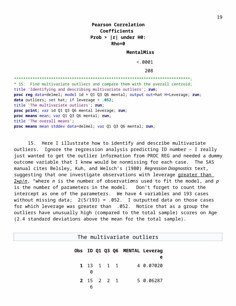
208****************************************************************************;* 15: Find multivariate outliers and compare them with the overall centroid;title 'Identifying and describing multivariate outliers'; run;proc reg data=delmel; model id = Q1 Q3 Q6 mental; output out=hat H=Leverage; run;data outliers; set hat; if leverage > .052;title 'The multivariate outliers'; run;proc print; var id Q1 Q3 Q6 mental leverage; run;proc means mean; var Q1 Q3 Q6 mental; run;title 'The overall means';proc means mean stddev data=delmel; var Q1 Q3 Q6 mental; run;

15. Here I illustrate how to identify and describe multivariate outliers. Ignore the regression analysis predicting ID number – I really just wanted to get the outlier information from PROC REG and needed a dummy outcome variable that I knew would be nonmissing for each case. The SAS manual cites Belsley, Kuh, and Welsch’s (1980) Regression Diagnostics text, suggesting that one investigate observations with leverage greater than 2 p / n , “where n is the number of observations used to fit the model, and p is the number of parameters in the model.” Don’t forget to count the intercept as one of the parameters. We have 4 variables and 193 cases without missing data; 2(5/193) = .052. I outputted data on those cases for which leverage was greater than .052. Notice that as a group the outliers have unusually high (compared to the total sample) scores on Age (2.4 standard deviations above the mean for the total sample).

The multivariate outliers

Obs

ID Q1 Q3 Q6 MENTAL

Leverage

1 130 1 1 1 4 0.07020

2 156 2 2 1 5 0.06287

3 164 1 4 1 7 0.13242

4 194 1 4 1 11 0.12275

5 200 1 3 1 10 0.05564

6 220 2 3 1 11 0.05773

7 224 1 1 1 4 0.07020

8 247 2 1 2 3 0.10134

9 275 2 3 1 11 0.05773

10 290 1 4 2 8 0.13172

14

Obs

ID Q1 Q3 Q6 MENTAL

Leverage

11 300 2 2 1 5 0.06287

12 310 2 4 2 11 0.13386

All three students aged 25 or older are included among the outliers.

Variable Label Mean (M-GM)/SD

Q1Q3Q6MENTAL

SexAgeCityCountry

1.5000000

2.6666667

1.2500000

7.5000000

0.18

2.40

-0.03

-1.33

The Overall Means

Variable Label Mean Std Dev

Q1Q3Q6MENTAL

SexAgeCityCountry

1.4095238

1.2666667

1.3904762

9.8808290

0.4929210

0.5831225

0.4890228

1.7944635

If you are using SPSS and do not want to export the data to SAS, you can screen the data in SPSS in much the same way you would in SAS. See my introductory lesson on data screening in SPSS.

Survey ScoundrelsA good while back my eldest daughter, who was a student at ECU, where I work, came into my

office and said something like “you are not going to believe what I just witnessed.” She went on to explain that she was waiting out in the hallway to get into a room where a survey was being conducted. Our students in introductory psychology are required to participate in research, and this was one of the activities that counted towards this requirement. My daughter explained to me that she had heard several other students talking about their plan to just answer the questions randomly, never even reading them, just to satisfy the requirement with minimal effort and get out of there.

My daughter was shocked, but I was not. I have seen this sort of behavior ever since I started doing research with humans. For a while I switched to doing research on rodents, who are better behaved than these humans. I have routinely included on questionnaires items such as “I frequently visit with aliens from other planets” and “I make all of my own clothes,” to help identify the scoundrels

15

who are not reading the questions. I also will repeat a few items and compare responses – for example, if an individual indicates that e is male on item 3 but female on item 56, something is likely amiss.

Recently I participated in an online survey where there were, peppered throughout the survey, items clearly designed to weed out those participants who were not reading the questions. Here is one example:

A respondent who answers anything other than “Strongly Disagree” to that last query is likely not reading the items or has some other characteristics that would make one wary of the data provided.

With surveys that are completed in a group, face-to-face, I have noticed the following behavior. The scoundrels complete the survey very quickly, and then sit there waiting until somebody gets up the nerve to hand it in after an unreasonably short period of time. Then the rest of the scoundrels hand in their responses as well. You might as well put all those data right into the trash can.

With online surveys you should also pay attention to the amount of time taken to complete the survey. Those who complete it in an unreasonably short period of time are likely scoundrels. There may also be problems with those who take an unreasonably long period of time.

There are, of course, external validity concerns related to culling out the data from scoundrels. Scoundrels account for a considerable proportion of our student population. When we attempt to generalize our results to the student population, we need keep that in mind.

Faculty at ECU conducting survey research are now encouraged to use items like this on all of their surveys. Here is a Facebook posting showing how some our students have reacted to this:

16

It might help to make the validity questions of about the same length as the other questions and vary their wording.

17

Code Booking

Computer data files often have many variables with short names. While it is good practice to make those names descriptive, it is even better practice to create a document that details what each variable is, and, for discrete variables, what the response options were and how they were coded. For example, variable “Gender” has response options 1 and 2. Is 1 female or male? [Sexist wisecrack: 1 is male, erect; 2 is female, curvy.] What is variable “IS?” Is it the “Intellectual Stimulation” subscale of your measure of transformational leadership, or the “Individualized Support” subscale of that measure, or might it be the “idiopathic seizures” variable?

Mark Bowler uses the term “code book” to refer to the document detailing what the variables are and what the value labels are, and he stresses, in his psychometrics class, the importance of creating such a document. I need to start stressing that too, in my stats classes. I tend to rely on the use of variable labels and value labels in SPSS and variable labels and value formats in SAS, and require these in assignments, but then many of my students drop this best practice when it comes to their own thesis or dissertation research. Sigh.

Here is an example of the sort of information that should be included in a code book:

Variable Name Question Value LabelsGPA Please provide your GPA: NoneClass Class (or faculty): 1=Freshman

2=Sophomore3=Junior4=Senior

Age Age: NoneSex Sex: 1=Male

2=FemaleRace Race: 1=Caucasian

2=Not CaucasianAccess_Cellphone Do you own a cellphone? 1=Yes

2=NoAccess_Desktop Do you have access to a computer or

laptop?0=No1=Yes

Approp_CP_Calls_Check_Messages Using a cell phone to make calls or check messages in class is never appropriate.

1=Strongly Disagree2=Somewhat Disagree3=Neither Agree nor Disagree4=Somewhat Agree5=Strongly Agree

Approp_CP_Send_Text_Check_Email_Never Using a cell phone to send text messages or check email in class is never appropriate.

1=Strongly Disagree … 2,3,4 …5=Strongly Agree

Approp_CP_Send_Text_Ck_Email_Lecture Using a cell phone to send text messages or check email in class is appropriate when the lecture is not interesting.

1=Strongly Disagree … 2,3,4 …5=Strongly Agree

18

Validity_1 Some people randomly answer questions, without even reading them. To detect such misbehavior, we employ validity questions. Please mark "Somewhat Disagree" for this question.

1=Strongly Disagree … 2,3,4 …5=Strongly Agree

Approp_CP_If_Not_Talking_Beeping

Cell phone use in class is appropriate only if it does not involve talking, beeping, or other noises.

1=Strongly Disagree … 2,3,4 …5=Strongly Agree

Approp_CP_Done_Quietly Cell phone use in class is appropriate only if it is done quietly and the phone is being used to look up information that is relevant to the class material being discussed.

1=Strongly Disagree … 2,3,4 …5=Strongly Agree

Drop-Down Problems with Internet Surveys

One of my brilliant graduate students gathered data with a Qualtrics survey. A drop-down box was employed for the question about respondent’s age, where option 1 was 18 years old, option 2 was 19 years old, and so on. These data were then treated as age in years. Such drop-down boxes have numerous problems. Some respondents are accustomed to using a scroll wheel to move down a page, but, if a drop box is open, scrolling that wheel will change the answer to the question, and this is likely more of a problem with very long drop-downs, where the respondent is likely not to notice that the answer has been changed. The drop-down in question here had at least 52 response options.

One way to avoid this drop-down problem is to have the respondents provide a plain text answer – for example, entering “47” instead of selecting the 47 drop-down option. When doing this, you must make it very clear that the entry must be digits, not alphanumeric – otherwise, some will enter “forty-seven” or :47 years and 69 days.” Sigh.

ReferenceIrwin, J.R., & McClelland, G.H. (2003). Negative consequences of dichotomizing continuous predictor

variables. Journal of Marketing Research, 40, 366-371.

Recommended ReadingUsing SPSS to Screen Data 

Dichotomizing Continuous Variables -- a bad idea

Reducing Negative Skewness

Replacing Missing Scores on Items Within a Scale -- Person Mean Imputation

Return to Wuensch’s Statistics Lessons Page

Copyright 2018, Karl L. Wuensch - All rights reserved.

19