Data Resource Profile: The Russia Longitudinal Monitoring ... cohort IntlJEpie2016.pdf · Polina...
26
Data Resource Profile Data Resource Profile: The Russia Longitudinal Monitoring Survey—Higher School of Economics (RLMS-HSE) Phase II: Monitoring the Economic and Health Situation in Russia, 1994–2013 Polina Kozyreva, 1 Mikhail Kosolapov 2 and Barry M. Popkin 3 * 1 Center for Longitudinal Studies, National Research University Higher School of Economics and Institute of Sociology, Russian Academy of Sciences, Moscow, Russia, 2 Institute of Sociology, Russian Academy of Sciences and Independent Research Center “Demoscope”, and National Research University Higher School of Economics, Moscow, Russia and 3 Carolina Population Center and Gillings School of Global Public Health, University of North Carolina, Chapel Hill, NC, USA *Corresponding author. Carolina Population Center, University of North Carolina, 137 East Franklin St, Chapel Hill, NC 27516, USA. E-mail: [email protected] Accepted 9 December 2015 Why was the data resource set up? The Russian Longitudinal Monitoring Survey (RLMS) was initially created by the G-7 countries in 1992 as a way to obtain objective nationally representative data on the so- cial, health and economic situation in Russia. It was estab- lished to mirror a multipurpose survey—the China Health and Nutrition Survey 1 —and provide in-depth reliable raw data on Russia, accessible for the first time to both Russian and global scholars and institutions. This was instituted in the period following January 1992, when the Russian Federation introduced a series of sweeping economic re- forms, including eliminating most food and reducing fuel and other subsidies, using freely fluctuating market prices, privatizing many state enterprises and working to create a growing private sector with private land ownership. The RLMS was created because the existing data, includ- ing a Family Budget Survey, were deemed unreliable, and adequate dietary, anthropometric and various other health- related behaviours were not measured in a nationally repre- sentative manner. These problems led to the initial Phase I survey of four rounds (I–IV) which was discontinued and is described in Supplement 1 (available as Supplementary data at IJE online). This was the first nationally representative random sample of economic and health data ever collected in Russia, with all earlier sampling based on quotas from en- terprises and other organizations. The ongoing longitudinal survey began in 1994 with the Phase II survey. In 2010, the Higher School of Economics (HSE) brought a number of the senior RLMS scholars onto its faculty and began to provide funding for the RLMS. Supplementary funding for subsequent nutrition and health-related data came from the University of North Carolina. At this time a decision was made to change the name to the RLMS-HSE. Data resource basics for the phase II survey Sample design Phase II The target sample size was set at 4 000 households. A multistage probability sample of households was V C The Author 2016; all rights reserved. Published by Oxford University Press on behalf of the International Epidemiological Association 1 International Journal of Epidemiology, 2015, 1–7 doi: 10.1093/ije/dyv357 Data Resource Profile Int. J. Epidemiol. Advance Access published February 13, 2016 by guest on February 14, 2016 http://ije.oxfordjournals.org/ Downloaded from
Transcript of Data Resource Profile: The Russia Longitudinal Monitoring ... cohort IntlJEpie2016.pdf · Polina...

Data Resource Profile
Data Resource Profile: The Russia Longitudinal
Monitoring Survey—Higher School of
Economics (RLMS-HSE) Phase II: Monitoring
the Economic and Health Situation in Russia,
1994–2013
Polina Kozyreva,1 Mikhail Kosolapov2 and Barry M. Popkin3*
1Center for Longitudinal Studies, National Research University Higher School of Economics and
Institute of Sociology, Russian Academy of Sciences, Moscow, Russia, 2Institute of Sociology, Russian
Academy of Sciences and Independent Research Center “Demoscope”, and National Research
University Higher School of Economics, Moscow, Russia and 3Carolina Population Center and Gillings
School of Global Public Health, University of North Carolina, Chapel Hill, NC, USA
*Corresponding author. Carolina Population Center, University of North Carolina, 137 East Franklin St, Chapel Hill, NC
27516, USA. E-mail: [email protected]
Accepted 9 December 2015
Why was the data resource set up?
The Russian Longitudinal Monitoring Survey (RLMS) was
initially created by the G-7 countries in 1992 as a way to
obtain objective nationally representative data on the so-
cial, health and economic situation in Russia. It was estab-
lished to mirror a multipurpose survey—the China Health
and Nutrition Survey1—and provide in-depth reliable raw
data on Russia, accessible for the first time to both Russian
and global scholars and institutions. This was instituted in
the period following January 1992, when the Russian
Federation introduced a series of sweeping economic re-
forms, including eliminating most food and reducing fuel
and other subsidies, using freely fluctuating market prices,
privatizing many state enterprises and working to create a
growing private sector with private land ownership.
The RLMS was created because the existing data, includ-
ing a Family Budget Survey, were deemed unreliable, and
adequate dietary, anthropometric and various other health-
related behaviours were not measured in a nationally repre-
sentative manner. These problems led to the initial Phase I
survey of four rounds (I–IV) which was discontinued and is
described in Supplement 1 (available as Supplementary data
at IJE online). This was the first nationally representative
random sample of economic and health data ever collected
in Russia, with all earlier sampling based on quotas from en-
terprises and other organizations.
The ongoing longitudinal survey began in 1994 with the
Phase II survey. In 2010, the Higher School of Economics
(HSE) brought a number of the senior RLMS scholars onto
its faculty and began to provide funding for the RLMS.
Supplementary funding for subsequent nutrition and
health-related data came from the University of North
Carolina. At this time a decision was made to change the
name to the RLMS-HSE.
Data resource basics for the phase II survey
Sample design Phase II
The target sample size was set at 4 000 households. A
multistage probability sample of households was
VC The Author 2016; all rights reserved. Published by Oxford University Press on behalf of the International Epidemiological Association 1
International Journal of Epidemiology, 2015, 1–7
doi: 10.1093/ije/dyv357
Data Resource Profile
Int. J. Epidemiol. Advance Access published February 13, 2016 by guest on February 14, 2016
http://ije.oxfordjournals.org/D
ownloaded from

employed to get a nationally representative sample for the
Russian Federation. First, a list of 1850 consolidated
raions (administrative-territorial districts), containing
95.6% of the population, was created to serve as primary
sampling units (PSUs). These were allocated into 38 strata
based largely on geographical factors and level of urban-
ization, but also based on ethnicity where there was sali-
ent variability. Three very large population units were
selected with certainty: Moscow city, Moscow Oblast and
St Petersburg city constituted self-representing (SR) strata.
The remaining non self-representing raions (NSR) were
allocated to 35 equal-sized strata. The total of 98 PSUs
were selected: 63 PSUs in three self-representing strata
and 35 PSUs in the rest non-representative strata. In
urban areas of the selected PSUs, secondary sampling
units (SSUs) were defined by the boundaries of census
enumeration districts. In rural areas, villages were com-
piled to serve as SSUs.
This was designed as an annual survey. Two years were
missed, 1997 and 1999, due to funding lapses between
1994 and 2014. The sample is described in more detail in
Supplement 2, Phase II (available as Supplementary data at
IJE online) and on the RLMS-HSE websites [http://www.
cpc.unc.edu/projects/rlms-hse/project/sampling].
In both urban and rural substrata, interviewers were
required to visit each selected dwelling up to three times to
secure the interviews. They were not allowed to make sub-
stitutions of any sort. ‘Household’ was defined as a group
of people who live together in a given domicile and share
common income and expenditures. Households were also
defined to include unmarried children, 18 years of age or
younger, who were temporarily residing outside the domi-
cile at the time of the survey.
The interviewer then conducted individual interviews
with as many household members aged 14 and older as
possible, acquiring data about their individual activities
and health. Data for children aged 13 and younger were
obtained from adults in the household. This provided a
probability sample of Russian individuals without special
weighting at baseline.
Nationally representative sample
The sample frame was essentially based on dwellings. In
conducting rounds VI–XXII, interviewers in both urban
and rural areas attempted to conduct interviews in the
same dwellings that fell into the first round of Phase II,
round V sample. They returned to each round V dwelling
even if the household had refused to participate during pre-
vious rounds, and even if they found out that the house-
hold whom they interviewed in previous rounds had
moved to a new dwelling before the interview. In Moscow
and St Petersburg, where the greatest non-response and ac-
cordingly the greatest attrition rates of the sample were
observed, the sample was replenished several times and
this was undertaken once in a few other cities. Figure 1
provides the dynamics of sample sizes of Phase II and de-
scribes the series of replenishments that occurred over time
to get to the final RLMS-HSE sample size from the round
XXII in 2013.
0
10
20
1994 1995 1996 1998 2000 2001 2002 2003 2004 2005 2006 2007 2008 2009 2010 2011 2012 2013
Sam
ple
size
K
N of Individuals in Total Sample*
N of Households in National representative Sample****
N of Households in Total Sample***
N of individuals in National representative Sample**
####
Figure 1. The dynamics of sample sizes Phase II RLMS-HSE2001. The nationally representative sample is followed by interviewing households and
individuals residing at the addresses of 1994 sample and addresses of replenishments. The total sample includes in addition the movers (households
or individuals who moved to new units for any reason, and were followed). #Replenishments: 2000, replenishment samples in Moscow and St
Petersburg, 2003: replenishment of the region within a stratum in 2003 (Novosibirsk region instead of Khanty-Mansiisk region); 2006, replenishment
to 1994 sample in most regions; 2010, a 50% increase in sample size following an identical sample selection approach.
*All individuals, participating in a given round, including movers who were followed. **Only individuals residing at the addresses of 1994 sample
and addresses of replenishment. ***All households participating in a given round, including movers who were followed. ****Only households resid-
ing at the addresses of 1994 sample and addresses of replenishment.
2 International Journal of Epidemiology, 2015, Vol. 0, No. 0
by guest on February 14, 2016http://ije.oxfordjournals.org/
Dow
nloaded from

Longitudinal cohort
The original sampling plan did not call for households to
be followed if they moved from the round V (1994) sample
dwelling unit. Likewise, individual household members
who moved away were not to be followed. After round VII
(1996), all individuals and households were followed when
they moved out of the household units (families, separated,
children got married, and so on) to live in the same second-
ary sampling unit (SSU) or move into one of the PSUs in
the sample. This created the current longitudinal cohort.
We attempted to find households who moved in the 1994–
96 period also.
Multilevel design
An array of contextual economic, demographic, social and
built environment infrastructure and related data are col-
lected for each of the smallest sampling units or local com-
munities (essentially SSUs or villages).
In all rounds of Phase II, questionnaires were obtained
from over 97% of the individuals listed on the household
rosters. The distribution of household size in the sample,
within both rural and urban localities, corresponds well to
the figures from the Russian census during all rounds of
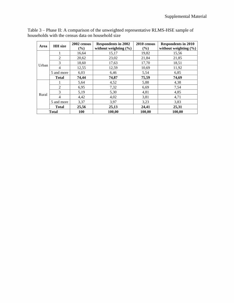
the survey (Supplement 2, Table 3, available as
Supplementary data at IJE online). Bear in mind that sin-
gle-member households are excluded from the comparison
because the census includes many institutionalized people,
whereas our sample explicitly excludes them. Thus, there
is no valid basis for comparison.
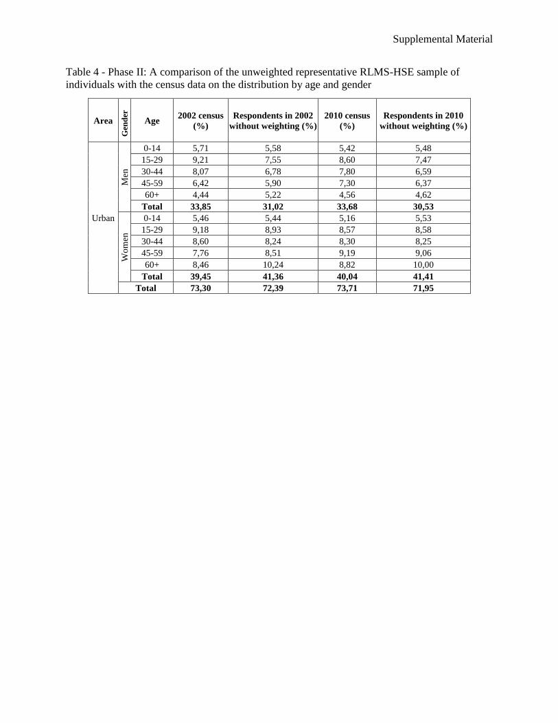
The multivariate distribution of the sample by sex, age,
education and urban-rural location compares quite well
with the corresponding multivariate distributions of the
nearest census data (Supplement 2, Tables 4 and 5, avail-
able as Supplementary data at IJE online). There are usu-
ally the differences of only 1–2 percentage points between
these distributions. The ethnic composition of the sample
throughout all rounds also corresponds to the census fig-
ures, having about 86% of Russians, 2.4% of Tatars and
10% of other nationalities.
Response rates
The household response rate in round V (which was the
first round of Phase II) exceeded 87.6% (for more detail see
Supplement 2, Tables 6 and 7, available as Supplementary
data at IJE online). Table 1 shows that over half of the
households participated in 10 rounds of RLMS-HSE, and
for individuals about half participated in eight rounds. This
creates a good basis for longitudinal analysis.
The response rates varied across PSUs, depending on
the proportion of households in rural areas. Obviously, in
Moscow and St Petersburg, respondents and household re-
sponse rates are substantially lower than in the Russian
Federation as a whole and, of course, the whole of Russia
without these two cities (Supplement 2, Tables 6 and 7).
However, since this situation was expected and has been
Table 1. The duration of participation in the survey (participation rate) for 1994 households and individuals (including separated
or moved out) 1994–2013
Rounds participated Household Individual
Percentage Cumulative percentage Percentage Cumulative percentage
All 18 rounds 26.14 26.14 16.50 16.50
Seventeen rounds 6.59 32.73 6.18 22.68
Sixteen rounds 3.55 36.28 3.80 26.48
Fifteen rounds 2.74 39.02 3.46 29.95
Fourteen rounds 2.74 41.76 2.92 32.87
Thirteen rounds 2.77 44.53 2.69 35.56
Twelve rounds 2.67 47.19 2.95 38.51
Eleven rounds 3.22 50.42 2.96 41.47
Ten rounds 3.12 53.53 2.93 44.40
Nine rounds 2.74 56.28 3.08 47.48
Eight rounds 2.99 59.27 3.21 50.69
Seven rounds 2.92 62.19 3.22 53.91
Six rounds 3.19 65.38 3.90 57.80
Five rounds 3.47 68.86 4.09 61.90
Four rounds 5.69 74.54 6.32 68.22
Three rounds 6.99 81.53 8.97 77.19
Two rounds 6.67 88.20 8.32 85.51
One round 11.80 100.00 14.49 100.00
International Journal of Epidemiology, 2015, Vol. 0, No. 0 3
by guest on February 14, 2016http://ije.oxfordjournals.org/
Dow
nloaded from

adjusted in oversampling procedures, the actual proportion
of completed household interviews compares well to the
proportion of the population in each stratum.
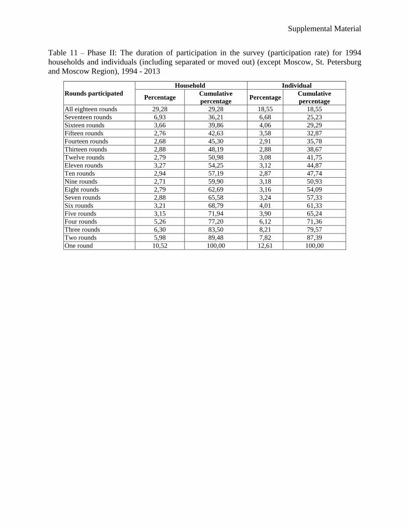
Since the highest non-response rate occurred in
Moscow and St Petersburg, the duration of participation in
the survey in these two cities was the lowest (Supplement
2, Tables 8–11, available as Supplementary data at IJE
online).
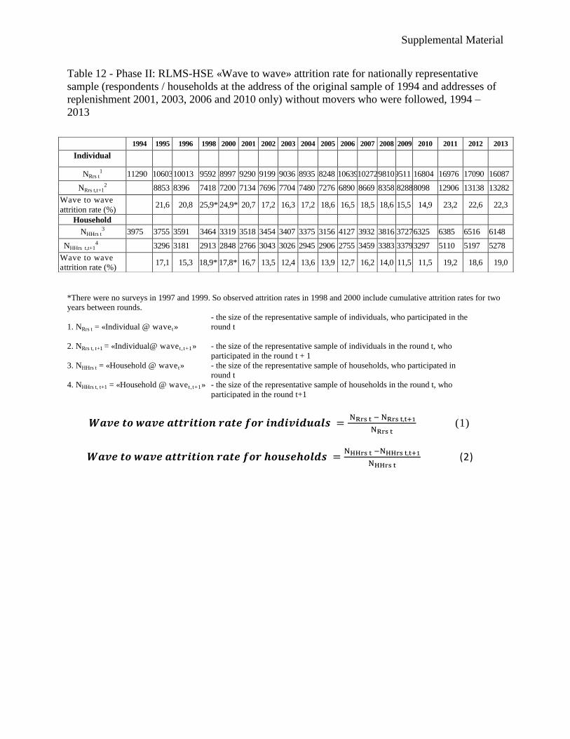
Attrition rates
One of the most important questions is: ‘How misleading
would it be to conduct pure panel analysis of households
and individuals observed in any set of consecutive rounds?’
The obvious problem is that, by definition, pure panel ana-
lysis can include only those who continue to reside in the
original sample dwelling units and participate in this set of
consecutive rounds. To evaluate the possibility of such
analysis, it is necessary to calculate attrition rates for any
such sequence of rounds. As an example, we present calcu-
lations for two most popular types of attrition rates
(Supplement 2, Tables 12–14, available as Supplementary
data at IJE online), namely wave-to-wave and baseline-on-
wave attrition rates for individuals and households. For all
18 rounds, only about 29% of households and 19% of in-
dividuals continued to participate (1994–2014) but, if we
look at the first 10 years, the results were about 60% and
51%, respectively (rounds 1–9) (Supplementary Table 12).
Table 2 presents death rates for the initial 1994 partici-
pants. Overall, 12.8% have passed away.
Data collected
Throughout the entire set of surveys, very detailed basic
household and individual data have been collected. Table 3
details this set of economic, labour force, demographic,
education, and related socioeconomic data. The full set of
English and Russian survey instruments are available on
the two RLMS-HSE websites. The household and individ-
ual core socioeconomic data are extremely detailed. They
contain classic income and expenditures data on all catego-
ries, from weekly food purchases to consumer durables.
The demographic data provide a classic triangle of the rela-
tionships of each person with each other within the house-
hold. The asset data include all sorts of details on
household and other assets. The employment information
is in-depth for multiple jobs with detail on type of employ-
ment, earnings, hours and ownership status (public, pri-
vate, joint) and provides the four-digit International
Labour Organization occupation code. Both actual and
perceived quality of life questions are interspersed.
Health data: for each wave, detailed data on alcohol
and smoking were obtained. Health service use data are
also collected but not in great detail. For selected rounds,
direct measurement of weight, height and waist circumfer-
ence were obtained (rounds V–XIV and XX). Also one-day
24-h recall dietary data were obtained in these rounds. In
only one round were replicates of a second day collected
for the sample.2,3 Nutrient intake levels are reported; how-
ever, actual detailed dietary data are not available as the
food composition table and data are controlled by a collab-
orator and were not made available.
There have been attempts to obtain biomarkers; unfortu-
nately, fasting blood or blood spot collection has been im-
possible as blood samples in any form cannot be taken out of
Russia, and it has not been possible to find a laboratory
equipped to handle full blood spot assays at reasonable cost
and reliability. These data have yet to be collected.
Spatial coordinates
For some time we attempted to use global positioning tech-
nology and collect coordinates for all major social and eco-
nomic and transport and health-related infrastructure as
well as household coordinates. Politically this was not feas-
ible until recently, and funding has not been obtained to
undertake this collection. However, the survey team is able
to provide (at cost) linkages of external data sets to the
RLMS-HSE contextual data by using deductive disclosure
controls to ensure anonymity of the identification of
communities.
Data resource use
Hundreds of English-language publications have arisen
from the RLMS-HSE data, authored by scholars globally.
In addition, there are thousands of Russian-language publi-
cations which are not accessible to most scholars globally.
Most of the focus has been on the poverty, economic, so-
cial and demographic data. These dietary and socioeco-
nomic data were used to create the Russian poverty line,
which established the pension level such that few
Table 2. Percentages of 1994 participants who died between 1994 and 2013
1995 1996 1998 2000 2001 2002 2003 2004 2005 2006 2007 2008 2009 2010 2011 2012 2013 Total
0.69 1.05 1.70 1.49 0.88 0.98 0.88 0.74 0.70 0.60 0.49 0.54 0.47 0.43 0.44 0.39 0.34 12.80
4 International Journal of Epidemiology, 2015, Vol. 0, No. 0
by guest on February 14, 2016http://ije.oxfordjournals.org/
Dow
nloaded from

pensioners in Russia are in poverty4,5 and almost none suf-
fer weight loss due to a lack of income.6 Related to the
poverty line has been extensive research on poverty by the
World Bank and many scholars globally.5,7,8
Alcohol intake has been subject to serious examination
by a vast number of scholars.9 One of the more interesting
issues is the skewed distribution with a small proportion of
men of all ages consuming about a half-litre of actual alco-
hol per day.10–12 The data showed a decreasing prevalence
of drinking during this period but an increase in the
amount of alcohol consumed by some members of this
population, and important cohort effects with older
Russians more likely to be drinking excessively.13 Partly
because of the high alcohol intake levels and the stresses of
the economic transformation, overall health, life expect-
ancy and mortality have been studied extensively.14–17 A
third topic is abortion, for which the RLMS-HSE results
produced much lower estimates than previous research.18
According to RLMS-HSE data, the abortion rate in 1994
was 56 per 1000 women aged 15–44, with a 95% confi-
dence interval of 6 12 per 1000, an estimate that varies
from that advanced by official sources and other studies.
Part of the reason for this difference is that the government
listed all miscarriages as induced abortions. In addition, we
used the advice of demographers who had studied this
issue for years (Professor Barbara Anderson, University of
Michigan, and others) to create confidential interviews on
this component.
Strengths and weaknesses
The major strengths of the RLMS-HSE are the national
representativeness, collection of very high quality sociode-
mographic and economic data, and the long follow-up.
The biggest weaknesses from the health side are the lack of
biomarkers and erratic collection of dietary and body com-
position data based on outside funding availability. And as
in all longitudinal surveys the attrition over time should be
considered while analyzing the data.
Data resource access
The bulk of the RLMS-HSE data are completely free and
available on the RLMS websites in English [http://www.
Table 3. RLMS-HSE survey components
Round Year of
collection
Core
household
SES dataa
Core
individual
SES datab
Time
budget
24-h diet/
weight-
height-WC
Child
care
Abortion/
family
planning
Sexual behaviour,
confidential
V 1994 X X X X X X
VI 1995 X X X X X X
VII 1996 X X X X X X
VIII 1998 X X X X X X
IX 2000 X X X X X
X 2001 X X X X X X
XI 2002 X X X X X
XII 2003 X X X X X X
XIII 2004 X X X X X
XIV 2005 X X X X X
XV 2006 X X X X
XVI 2007 X X X X
XVII 2008 X X X X
XVIII 2009 X X X X
XIX 2010–11 X X X X
XX 2011–12 X X X X X
XXI 2012–13 X X X X
XXII 2013–14 X X X X
WC, waist circumference.aThe core household data collected each year include: household composition/relationships; housing (structure, amenities, privatization, ownership); possession
of consumer durables; raising food on private plots; in-depth food, clothes and consumer durables during 3 months, savings, transfer payments, gifts to others,
utilities and many other expenditures; income from all wage and non-wage sources by public and private sector status, including transfer payments, gifts, stock
market, and drawing down savings; and details on non-payment of wages and losses due to bank closures.bThe core individual data (questions on children age < 14, answered by parents): these include place of birth, some migration, language, marital status; work
(primary, secondary, entrepreneur, independent, unofficial, unemployment, employment-seeking); years of work experience; willingness to be retrained; four-digit
occupational coding according to the International Labour Organization protocol; education (current and past); self-ratings of satisfaction, well-being, poverty,
relationship with others; use of medical services and medicines and insurance; childbearing and birth control (including child-bearing and abortion history); plans
included are smoking and alcohol in-depth blocks of questions.
International Journal of Epidemiology, 2015, Vol. 0, No. 0 5
by guest on February 14, 2016http://ije.oxfordjournals.org/
Dow
nloaded from

cpc.unc.edu/projects/rlms-hse/] and Russian and English
[www.hse.ru/rlms]. The sexual behaviour data are highly
confidential, as are spatial locations of sample recipients.
Institutional Review Board approval for each survey has
been provided by both the institutional review boards of
the University of North Carolina and the Higher School of
Economics. Contextual data require also special applica-
tions. To link other contextual measures to the RLMS-
HSE data, this must be done at cost by contacting the
Carolina Population Center.
Supplementary data
Supplementary data are available at IJE online.
AcknowledgmentsOur deepest debt goes to the late Dr Michael Swafford for his col-
laboration during the 1991–2001 period. Key collaborators of the
authors in this survey are: NamvarZohoori, Barbara Entwisle and
Lenore Kohlmeier, USA; Alexander Ivanov and Igor Dmitrichev,
Goskomstat; Svetlana Shalnova and Alexander Deev, RCPM;
Alexander Baturin and Arseni Martinchik, Institute of Nutrition,
Russian Academy of Medical Sciences. Leslie Kish and Steve
Heeringa of the University of Michigan were the senior US sampling
researchers for Phase II, and William Kalsbeek, University of North
Carolina at Chapel Hill, was the leading sampling scholar for Phase
I. Steve Heeringa has met with us four times since the beginning of
Phase II, to review the sampling with the US and Russian teams, and
decided on replenishment and expansion strategies to keep the sam-
ple statistically representative of the Russian Federation.
Consultants on various phases of the survey design work have
included Michael Berbaum of the University of Alabama, who was
instrumental (along with Michael Swafford) in adopting the initial
English design into Russian. Other survey researchers who have pro-
vided questionnaire design consultation include: Cynthia Kaplan
(University of California, Santa Barbara), Vladimir Treml (Duke
University) and Marina Mozhina (Institute of Socioeconomic
Problems of Population, Russian Academy of Sciences). A scientific
panel provided project advice for round V (the second phase of the
survey and start of the true longitudinal and nationally representa-
tive panels) and four subsequent rounds. Members of the panel
were: Barbara Anderson (University of Michigan), Donna Bahry
(Penn State University), Ward Kingkade (US Census Bureau) and
Vladimir Treml (Duke University). The entire group of laboratories,
headed by Polina Kozyreva and Michael Kosolopov and many staff
and doctoral students at CPC-UNC, has led a series of redesigns of
the survey. Phil Bardsley at UNC and a set of programmers at
Demoscope have created and continued the Web support for the sur-
vey, with no funding for data dissemination.
Funding
The first decade of funding was complex. Initially the G-7 team and
the Russian Federation concurred in organizing this survey, and the
World Bank was the lead agency to fund all aspects of the work.
Phase I, round 1, was funded by the World Bank, whereas Phase I,
rounds 2–4, were funded by both the World Bank and USAID. For
Phase II, rounds V–VIII obtained USAID funding with supplementary
support from NIH (R01-HD38700) and NSF (SBR-9223326).
Throughout, support came from the University of North Carolina,
Carolina Population Center (CPC) (5 R24 HD050924), and in later
years the Government of Sweden (Stockholm Institute of Transition
Economics), the Ford Foundation, the MacArthur Foundation, the
Pension Fund of the Russian Federation, along with some supplemen-
tary NIH funding. Most recently, since 2010 the National Research
University Higher School of Economics has provided core survey sup-
port. A variety of sources have funded ancillary surveys (e.g. the diet-
ary and body composition data in 2011 funded by CPC).
Conflict of interest: None declared.
References
1. Popkin BM, Du S, Zhai F, Zhang B. Cohort Profile: The China
Health and Nutrition Survey—monitoring and understanding
Profile in a nutshell
• The RLMS-HSE was established to create a nation-
ally representative survey to monitor the economic
and health impact of the massive set of reforms in
the Russian Federation.
• Established in 1992 (Phase I) and, for Phase II (dis-
cussed in depth here) in 1994, this annual survey is
both nationally representative plus has a longitu-
dinal component. Both collect multipurpose health
and economic studies with in-depth individual,
household and community contextual data collected
in all rounds.
• The 1994 and 2013 samples collected the data from
11 290 and 21 753 individuals and 3975 and 8149
households, respectively. A multistage sample with
98 primary sampling units (Moscow city, Moscow
Oblast and St Petersburg are self-representing) was
designed to represent the Russian Federation.
• The major data components are: economic (detailed
income, labour force behaviour and expenditures
data); demographic/sociological (household structure
and age-gender composition, background, education
and school behaviour); and health (24-h dietary re-
call, smoking, drinking activity, body mass index dir-
ect measurement).
• Data can be linked to other contextual datasets.
• The bulk of the RLMS-HSE data are completely free
and available on the UNC-CPC websites in English
[http://www.cpc.unc.edu/projects/rlms-hse/] and the
RLMS-HSE website in Russian and in English [http://
www.hse.ru/rlms/]. Selected confidentiality forms are
required for selected data such as sexual behaviour
of adolescents.
6 International Journal of Epidemiology, 2015, Vol. 0, No. 0
by guest on February 14, 2016http://ije.oxfordjournals.org/
Dow
nloaded from

socio-economic and health change in China, 1989-2011. Int J
Epidemiol 2010;39:1435–40.
2. Jahns L, Arab L, Carriquiry A, Popkin BM. The use of external
within-person variance estimates to adjust nutrient intake distri-
butions over time and across populations. Public Health Nutr
2005;8:69–76.
3. Jahns L, Carriquiry A, Arab L, Mroz TA, Popkin BM. Within-
and between-person variation in nutrient intakes of Russian
and US children differs by sex and age. J Nutr 2004;134:
3114–20.
4. Lokshin M, Harris KM, Popkin BM. Single mothers in Russia:
household strategies for coping with poverty. World Dev
2000;28:2183–98.
5. Lokshin M, Popkin BM. The emerging underclass in the Russian
Federation: income dynamics. Econ Dev Cult Change 1999;
47:803–29.
6. Stookey JD, Zohoori N, Popkin BM. Nutrition of elderly people
in China. Asia Pac J Clin Nutr 2000;9:243–51.
7. Lokshin M, Ravallion M. Welfare impacts of the 1998 financial
crisis in Russia and the response to the public safety net. Econ
Transit 2000;8:269–95.
8. Ravallion M, Lokshin M. Who wants to redistribute Russia’s
tunnel effect in the 1990s? J Public Econ 2000;76:87–104.
9. Zohoori N, Mroz TA, Popkin B et al. Monitoring the economic
transition in the Russian Federation and its implications for the
demographic crisis—The Russian Longitudinal Monitoring
Survey. World Dev 1998;26:1977–93.
10. Baltagi BH, Geishecker I. Rational alcohol addiction: evidence
from the Russian Longitudinal Monitoring Survey. Health Econ
2006;15:893–914.
11. Tapilina VS. How much does Russia drink: volume, dynamics
and differentiation of alcohol consumption. Russian Soc Sci Rev
2007;48:79–94.
12. Tekin E. Employment, wages, and alcohol consumption in
Russia. South Econ J 2004;71:397–417.
13. Zohoori N. Recent patterns of alcohol consumption in the
Russian elderly, 1992-1996. Am J Clin Nutr 1997;66:810–14.
14. Andreev EM, McKee M, Shkolnikov VM. Health expectancy in
the Russian Federation: a new perspective on the health divide in
Europe. Bull World Health Organ 2003;81:778–87.
15. Cockerham WC. Health lifestyles in Russia. Soc Sci Med 2000;
51:1313–24.
16. Perlman F, Bobak M. Socioeconomic and behavioral determin-
ants of mortality in posttransition Russia: a prospective popula-
tion study. Ann Epidemiol 2008;18:92–100.
17. Shkolnikov VM, Andreev EM, Anson J, Mesle F. The peculiar
pattern of mortality of Jews in Moscow, 1993–95. Popul Stud
2004;58:311–29.
18. Entwisle B, Kozyreva P. New estimates of induced abortion in
Russia. Stud Fam Plann 1997;28:14–23.
International Journal of Epidemiology, 2015, Vol. 0, No. 0 7
by guest on February 14, 2016http://ije.oxfordjournals.org/
Dow
nloaded from

Supplemental Material
Supplement 1. Phase I: The initial Russia Longitudinal Monitoring Survey
A. Motivation:
The lack of valid, reliable statistical data: From the 1950s through the 1990s, the
former Soviet Union and then the Russian Federation relied on the State Committee on Statistics
(Goskomstat) to provide it with information on income, expenditures, poverty, and employment
patterns. The major instrument to provide this information was the Consumer Budget Survey (or
often called the Family Budget Survey, FBS). This is essentially the equivalent of the income
and budget survey of the US Bureau of Labor Statistics or similar instruments in other countries.
There were significant problems related to the sampling, design, implementation, and use of the
FBS. Goskomstat has been collecting its own series of household income and consumption data
since the early 1950s in an effort to provide data for the planners of its command economy.
During the 1990s, Goskomstat continued to survey 49,000 households twice monthly. Although
this massive panel survey would seem to be an outstanding source of data on the material well-
being of Russian citizens, it suffered from serious flaws in sampling, questionnaire design,
training, quality controls, data entry and processing, and analysis.
The Sample: Since the economy at that date was organized around powerful economic
ministries until the onset of economic reform, the survey was originally based on a sample of
enterprises and organizations within each ministry. Even as a sample of households within
ministries, the sample was always problematic. There was no documentation of the use of
properly weighted standard probability procedures in the selection of enterprises, nor was there
any effort to allocate households regionally in a way that would properly support the detailed
oblast-level reports that have been routinely used as a basis for policy making. Russian policy
makers who took charge of the economic during the reform period following the creation of the
Russian Federation under Boris Yeltsin were acutely aware of the imprecision of their statistical
estimates, since standard errors were never reported and could not be properly calculated given
the procedures employed in drawing the sample.
Furthermore, even though the survey purports to represent households, the sample has
been based on a list of individual full-time workers in enterprises, not an enumeration of
households per se. This means, for example, that households with one worker in the economic
ministries (i.e., state sector) had only one third the probability of selection that households with
three such workers had (all else being equal). Households with no workers in the state sector had
no probability of falling into the sample. For example, a two-person household consisting of two
pensioners had no way of falling into the sample until Goskomstat appended a haphazard sample
of pensioners. It later made an effort to represent households supporting themselves with work in
the new private sector. However, this change did not adjust for the fact that the bulk of the
sample was not based on an enumeration of dwellings or households over the decades.
Unfortunately, even the longitudinal potential of the FBS data cannot be exploited
because a household drawn to replace another household that dropped out of the study is given
the same ID number as the one that dropped out. Consequently, in attempting to study change at
the level of individual households, one cannot determine whether observed differences over time
should be attributed to real change within one household or to substantively uninteresting change
reflecting the different households with the same ID involved in the survey at two points in time.
Questionnaire design: As noted already, the FBS used a variant of a classical income and
expenditure survey. It was designed to collect monthly income from workers who relied mainly

Supplemental Material
on wages from enterprises in addition to a set of subsidies and bonuses. The latter were collected,
but there was little attempt to quantify in-kind subsidies, and there was no attempt to collect
nonmarket production. It failed to capture the hidden economy of barter, private sector income
and employment, work outside the basic core public employment, and many other economic
activities. The FBS differed in that it was changed into a booklet into which families were
expected to record each expenditure and earning as they were received on a daily basis—a
remarkably tedious task. At the end of each month, the questionnaires were collected by an
interviewer who actually functioned as an auditor, making sure the numbers added up properly.
Data entry and processing: This was a centralized operation. Each oblast was provided
with software developed in the 1950s that entered the information and created a set of tables.
Verification of data entry was not performed. The tables were then sent to the next higher
administrative level for aggregation at a national level. Analysts at Goskomstat did not have
direct access to the FBS data tapes and could not analyze these rich data at the individual level or
in any manner not reported on the tables provided by each oblast. This lack of standardization of
data processing meant that it was impossible for Goskomstat to provide information in ways that
might be responsive to a wide range of demands by the public sector.
Analysis: Absence of detailed data has not only hindered the work of Goskomstat but
meant that there was little micro-information on the economy available for Russian economists
and others involved in policy analysis. Skills in microdata analysis were not developed. Rather,
Soviet scholars developed innovative and complex mathematical and theoretical frameworks
based on the limited secondary data, macro-information, and a large element of speculation.
B. PHASE I SURVEY
The RLMS was a household-based survey designed to address many of the deficiencies
of the Family Budget Survey. Initially this survey was implemented in conjunction with
Goskomstat. The new survey instrument was designed not only to address deficiencies of the
FBS but also to act as a multipurpose combination of income and expenditure, employment, and
health surveys. This instrument collected data necessary for a wide array of analyses, programs,
and policies critical to the design of social and economic programs and policies in the early
reform period.
Design and training were organized and led by the team of researchers of the Institute of
Sociology RAS, later created for RLMS realization the independent research center
"Demoscope"; funding and overall leadership came from the CPC-UNC team. This included a
fourth major person, Michael Swafford, who subsequently passed away. This team handled
questionnaire design, training, quality control, design of the data entry software.
Sample Design Phase I
The sampling for Phase I came from adviser William Kalsbeek (a sampling expert at
UNC-CH) and later with help from Leslie Kish, an eminent US scholar. The project developed a
replicated three-stage, stratified cluster sample of residential addresses excluding military, penal,
and other institutionalized populations. Briefly, in the first stage, a sample of 20 raions (PSU)
was selected; in the second, a sample of 10 voting districts was selected in each of these raions;
in the third, a sample of 36 households (not voters) was selected in each of these voting districts.
This yielded a target sample of 7,200 households. With nonresponse, the actual number of
households varied around 6,000 over the four rounds (see Tables 1 and 2). Weights and design
effects measures were created.

Supplemental Material
Four rounds (I–IV) were conducted within Phase I of RLMS.
--Tables 1 and 2 about here--
Members of the research group of the Institute of Sociology conducted elaborate checks
of the way the sample was drawn in each oblast, including direct checks of lists and households.
As a result of large-scale checks, the correctness of the field phase of the first wave of the
survey, conducted by Goskomstat, were marked by systematic violations of requirements for
RLMS technology. It was not possible, however, during the period of work with Goskomstat, to
get more than a small number of supervisors to actively check interviews on a day-to-day basis
and send back interviewers to correct problems. Ultimately a decision was made to end work
with Goskomstat.
Because of the questionable quality of the data and the sample, the inability to link
households over time, and the dummy cases, we recommended to users that these data not be
used, but we do provide them when requested. In contrast we have very high-quality Phase II
data handling and keep those data accessible online.

Supplemental Material
Supplement 2. Sample design for Phase II: The Russia Longitudinal Monitoring Survey-
Higher School of Economics
The sampling for Phase II came from a team led by Michael Swafford, Mikhail
Kosolapov, and Leslie Kish. This probability sample was designed to overcome three of the
shortcomings of the probability sample used in rounds I–IV (which was developed in a short
time frame under constraints imposed by Goskomstat).
First, a list of 2,029 consolidated raions was created to serve as primary sampling units
(PSUs). These were allocated into 38 strata based largely on geographical factors and level of
urbanization, but also on ethnicity where there was salient variability. As in many national
surveys involving face-to-face interviews, some remote areas were eliminated to contain costs.
From among the remaining 1,850 raions (containing 95.6% of the population), three very large
population units were selected with certainty: Moscow city, Moscow oblast, and St. Petersburg
city constituted self-representing (SR) strata. The remaining non-self-representing raions (NSRs)
were allocated to 35 equal-sized strata. One raion was then selected from each NSR stratum
using the method "probability proportional to size" (PPS).
All NSR strata have approximately equal sizes because they were purposefully designed
to improve the efficiency of estimates. As is often the case, we were obliged to use figures on the
population of individuals as a surrogate of population of eligible households because of the
unavailability of household figures in various regions. Although the target sample size was set at
4,000, the number of households drawn into the sample was inflated to 4,718 to allow for a
nonresponse rate of approximately 15%. The number of households drawn from each of the NSR
strata was approximately equal (averaging 108). However, because we expected response rates to
be higher in urban areas than in rural areas, the extent of oversampling varies. An initial sample
size was different for different NSRs. This also explains that the share of the original sample
attributable to three SR strata more that would have been allotted based on strict proportionality.
Since there was no consolidated list of households or dwellings in any of the 38 selected
PSUs, an intermediate stage of selection was introduced, as usual. The selection of second-stage
units (SSUs) differed depending on whether the population was urban (located in cities and
"villages of the city type," known as PGTs) or rural (located in villages). That is, within each
selected PSU the population was stratified into urban and rural substrata, and the target sample
size was allocated proportionately to the two substrata.
In rural areas of the selected PSUs, a list of all villages was compiled to serve as SSUs.
The list was ordered by size and (where salient) by ethnic composition. Again, under the
standard principles of PPS, once the required number of villages was selected, an equal number
of households in the sample (10) was allocated to each village. Since villages maintain very
reliable lists of households, in each selected village the 10 households were selected
systematically from the household list. In urban areas, SSUs were defined by the boundaries of 1989 census enumeration
districts, if possible. If the necessary information was not available, 1994 microcensus
enumeration districts and voting districts were employed in decreasing order of preference. Since
census enumeration districts were originally designed to be roughly equal in population size, one
district was selected systematically without using PPS for each 10 households required in the
sample. In the few cases where voting districts were used, to compensate for the marked
variation in population size PPS was employed to select one voting district for each of the 10
households. Given the lack of reliable official lists of households within the urban SSUs, we
were obliged to develop the list of households from which 10 were selected. First, a list of

Supplemental Material
dwellings was made. Then, the required number of households was drawn systematically,
starting with a random selection in the first interval. The initial Phase II, beginning with round V in 1994, interviewed 3,975 households and
11,290 individuals. Beginning with round VII we actually created two samples—the nationally
representative panel and then the longitudinal sample including all movers, households, and
individuals that were possible. As each household entered the RLMS, they were followed if they
moved and became part of the longitudinal sample.
A comparison of the unweighted representative RLMS-HSE sample of households
and individuals with the census data.
--Tables 3, 4 and 5 about here--
Response Rates We present response rates for the two samples. The first is the response rate for nationally
representative sample of households, which are households residing at the address of the original
sample of 1994 and addresses of replenishment 2006 and 2010.
--Table 6 about here--
Since there have been replenishment in RLMS-HSE sample over 20 years, it is difficult
to compare response rates between rounds before and after replenishment. So we divided the
columns for 2006 and 2010 in two parts.
--Table 7 about here--
To analyze response rate dynamics, we calculated the second type of the response rate for
sample of households that reside at the address of the original sample of 1994. We excluded new
addresses added in 2006 and 2010.
The duration of participation in the survey (participation rate) 1994-2013 is
presented in tables 8-11.
--Tables 8-11 about here--
Attrition Rates
We provide much more detail on the sample attrition. Sample attrition due to
nonresponse cannot be avoided. In longitudinal studies, it is very important to be able to assess
attrition effects on simulated "pure panel" analysis.
--Tables 12-14 about here--

Supplemental Material
Table 1 - Phase I: Sample size – individuals and households Survey Dates July-Oct 1992 Dec 1992-Mar 1993 Jan-Sept 1993 Oct 1993-Jan 1994
Individual (no) 16,623 15,013 15,030 14,466
Household (no) 6,333 6,043 5,836 5,766

Supplemental Material
Table 2 - Phase I: Longitudinal cohorts: RLMS response rates at the individual and household
levels. Survey Dates July-Oct 1992 Dec 1992-Mar 1993 Jan-Sept 1993 Oct 1993-Jan 1994
Individual
N 16,623 15,013 15,030 14,466
Response rate (%)* 100 90.3 90.4 87.0
Household
N 6,333 6,043 5,836 5,766
Response rate (%)* 100 95.4 92.1 91.0
Supplemental Material
Table 3 – Phase II: A comparison of the unweighted representative RLMS-HSE sample of
households with the census data on household size
Area HH size 2002 census
(%)
Respondents in 2002
without weighting (%)
2010 census
(%)
Respondents in 2010
without weighting (%)
Urban
1 16,64 15,17 19,82 15,56
2 20,62 23,02 21,84 21,85
3 18,60 17,63 17,70 18,51
4 12,55 12,59 10,69 11,92
5 and more 6,03 6,46 5,54 6,85
Total 74,44 74,87 75,59 74,69
Rural
1 5,64 4,52 5,88 4,38
2 6,95 7,32 6,69 7,54
3 5,19 5,30 4,81 4,85
4 4,42 4,02 3,81 4,71
5 and more 3,37 3,97 3,23 3,83
Total 25,56 25,13 24,41 25,31
Total 100 100,00 100,00 100,00
Supplemental Material
Table 4 - Phase II: A comparison of the unweighted representative RLMS-HSE sample of
individuals with the census data on the distribution by age and gender
Area G
end
er
Age 2002 census
(%)
Respondents in 2002
without weighting (%)
2010 census
(%)
Respondents in 2010
without weighting (%)
Urban
Men
0-14 5,71 5,58 5,42 5,48
15-29 9,21 7,55 8,60 7,47
30-44 8,07 6,78 7,80 6,59
45-59 6,42 5,90 7,30 6,37
60+ 4,44 5,22 4,56 4,62
Total 33,85 31,02 33,68 30,53
Wo
men
0-14 5,46 5,44 5,16 5,53
15-29 9,18 8,93 8,57 8,58
30-44 8,60 8,24 8,30 8,25
45-59 7,76 8,51 9,19 9,06
60+ 8,46 10,24 8,82 10,00
Total 39,45 41,36 40,04 41,41
Total 73,30 72,39 73,71 71,95

Supplemental Material
Table 5 - Phase II: A comparison of the unweighted representative RLMS-HSE sample of
individuals with the census data on the distribution by education**
Area
Gen
der
Education 2002 census
2002
census
(%)
Respondents
in 2002
Respondent
s in 2002
(%)
2010 census
2010
census
(%)
Responde
nts in 2010
(%)
Urban
Men
Secondary education
and lower 14292866 35,6 918 39,3 11743874 30,2 1398 33,1
Post-secondary non-
tertiary education 18319797* 45,6 953 40,8 17007707* 43,8 1795 42,5
Tertiary education and
higher 7562779 18,8 464 19,9 10077326 26,0 1028 24,4
Subtotal 40175442 100,0 2334 100,0 38828907 100,0 4221 100,0
n/a 635363 8 1536590 4
Total 40810805 2343 40365497 4225
Wo
men
Secondary education
and lower 17510306 36,0 1316 39,9 13704010 28,5 1936 32,0
Post-secondary non-
tertiary education 21606895* 44,4 1306 39,6 20369050* 42,4 2439 40,3
Tertiary education and
higher 9500789 19,5 676 20,5 13941633 29,0 1675 27,7
Subtotal 48617990 100,0 3294 100,0 48014693 100,0 6051 100,0
n/a 690821 9 1800333 2
Total 49308811 3308 49815026 6053
Total 90119616 5651 90180523 10278
Rural
Men
Secondary education
and lower 7542747 51,7 558 60,5 7743816 53,5 905 53,0
Post-secondary non-
tertiary education 5984727* 41,1 304 33,0 5243019* 36,2 652 38,2
Tertiary education and
higher 1050047 7,2 60 6,5 1488820 10,3 150 8,8
Subtotal 14577521 100,0 921 100,0 14475655 100,0 1707 100,0
n/a 18752 4 89896 5
Total 14596273 925 14565551 1712
Wo
men
Secondary education
and lower 9175736 55,4 685 59,4 8249695 50,5 1007 46,9
Post-secondary non-
tertiary education 6124354* 37,0 367 31,8 6037598* 37,0 842 39,2
Tertiary education and
higher 1264784 7,6 101 8,8 2032928 12,5 297 13,8
Subtotal 16564874 100,0 1153 100,0 16320221 100,0 2146 100,0
n/a 19472 6 87632 1
Total 16584346 1159 16407853 2147
Total 31180619 2084 30973404 3859
Total 121300235 7735 121153927 14137
* Including incomplete higher education, i.e. there are individuals who entered the university but have not received
a degree.
** Only respondents aged 15+. This design was applied due to the census data restriction.

Supplemental Material
Table 6 - Phase II. RLMS-HSE response rate for nationally representative sample of households,
that are households residing at the address of the original sample of 1994 and addresses of
replenishment 2006 and 2010 (without movers who were followed), 1994 – 2013, %
1994 1995 1996 1998 2000 2001 2002 2003 2004 2005 2006 2006* 2006** 2007 2008 2009 2010 2010* 2010** 2011 2012 2013
All 87,6 82,1 79,4 77,7 75,1 57,9 57,3 54,8 55,0 51,1 45,6 51,9 32,7 43,2 42,2 44,4 41,8 50,9 27,6 38,7 37,3 37,7
All regions
except Moscow and
Saint
Petersburg
91,8 87,3 84,9 83,4 82,0 80,4 78,8 76,8 76,4 72,6 56,1 70,3 35,3 53,7 52,5 52,7 49,0 57,8 33,6 44,8 46,3 45,3
Only Moscow
and Saint
Petersburg
62,9 51,7 47,0 42,6 32,7 20,5 21,8 17,8 18,9 15,8 18,8 19,3 15,9 18,1 16,8 21,0 18,5 23,8 12,7 17,3 16,2 15,9
* Only households residing at addresses that participated in the survey earlier
** Only households residing at new addresses

Supplemental Material
Table 7 - Phase II. RLMS-HSE response rate for sample of households that are households
residing at the address of the original sample of 1994 without movers, 1994 – 2013 %
1994 1995 1996 1998 2000 2001 2002 2003 2004 2005 2006 2007 2008 2009 2010 2011 2012 2013
All 87,6 82,1 79,4 77,7 75,1 57,9 57,3 54,8 55,0 51,1 51,9 49,1 47,9 46,6 47,8 49,9 50,1 47,7
All regions except Moscow and St.
Petersburg
91,8 87,3 84,9 83,4 82,0 80,4 78,8 76,8 76,4 72,6 70,3 67,9 65,8 64,3 65,4 62,4 63,1 60,1
Only Moscow and St.
Petersburg 62,9 51,7 47,0 42,6 32,7 20,5 21,8 17,8 18,9 15,8 19,3 18,3 17,9 17,6 18,0 21,1 20,8 19,2

Supplemental Material
Table 8 - Phase II: The duration of participation in the survey (participation rate) for 1994
households and individuals (including separated or moved out) (Moscow), 1994 – 2013*
Rounds participated
Household Individual
Percentage Cumulative
percentage Percentage
Cumulative
percentage
All eighteen rounds 4,17 4,17 2,22 2,22
Seventeen rounds 4,92 9,09 3,33 5,56
Sixteen rounds 2,65 11,74 2,22 7,78
Fifteen rounds 2,65 14,39 2,50 10,28
Fourteen rounds 2,27 16,67 3,06 13,33
Thirteen rounds 0,76 17,42 0,97 14,31
Twelve rounds 2,27 19,70 2,78 17,08
Eleven rounds 2,27 21,97 1,11 18,19
Ten rounds 2,27 24,24 2,50 20,69
Nine rounds 3,79 28,03 2,22 22,92
Eight rounds 3,79 31,82 3,33 26,25
Seven rounds 2,65 34,47 2,50 28,75
Six rounds 2,27 36,74 2,50 31,25
Five rounds 6,82 43,56 5,56 36,81
Four rounds 10,98 54,55 8,61 45,42
Three rounds 17,42 71,97 19,44 64,86
Two rounds 10,98 82,95 12,36 77,22
One round 17,05 100,00 22,78 100,00

Supplemental Material
Table 9 - Phase II: The duration of participation in the survey (participation rate) for 1994
households and individuals (including separated or moved out) (St. Petersburg), 1994 – 2013*
Rounds participated
Household Individual
Percentage Cumulative
percentage Percentage
Cumulative
percentage
All eighteen rounds 2,01 2,01 1,08 1,08
Seventeen rounds 3,36 5,37 1,73 2,81
Sixteen rounds 1,34 6,71 0,43 3,25
Fifteen rounds 2,01 8,72 1,95 5,19
Fourteen rounds 3,36 12,08 2,16 7,36
Thirteen rounds 3,36 15,44 1,08 8,44
Twelve rounds 2,01 17,45 0,65 9,09
Eleven rounds 2,68 20,13 1,73 10,82
Ten rounds 2,68 22,82 1,95 12,77
Nine rounds 0,00 22,82 0,43 13,20
Eight rounds 3,36 26,17 2,16 15,37
Seven rounds 2,68 28,86 3,03 18,40
Six rounds 4,03 32,89 4,76 23,16
Five rounds 3,36 36,24 4,98 28,14
Four rounds 6,71 42,95 6,49 34,63
Three rounds 7,38 50,34 9,31 43,94
Two rounds 14,09 64,43 12,99 56,93
One round 35,57 100,00 43,07 100,00

Supplemental Material
Table 10 - Phase II: The duration of participation in the survey (participation rate) for 1994
households and individuals (including separated or moved out) (Moscow Region), 1994 – 2013*
Rounds participated
Household Individual
Percentage Cumulative
percentage Percentage
Cumulative
percentage
All eighteen rounds 20,2 20,20 12,00 12,00
Seventeen rounds 5,6 25,76 4,80 16,80
Sixteen rounds 4,5 30,30 4,20 21,00
Fifteen rounds 3,0 33,33 4,00 25,00
Fourteen rounds 4,0 37,37 3,60 28,60
Thirteen rounds 3,0 40,40 3,00 31,60
Twelve rounds 1,5 41,92 2,80 34,40
Eleven rounds 4,0 45,96 3,60 38,00
Ten rounds 7,6 53,54 5,60 43,60
Nine rounds 4,0 57,58 4,80 48,40
Eight rounds 5,1 62,63 4,80 53,20
Seven rounds 4,0 66,67 4,00 57,20
Six rounds 3,5 70,20 3,00 60,20
Five rounds 4,5 74,75 4,80 65,00
Four rounds 5,1 79,80 6,80 71,80
Three rounds 4,5 84,34 8,20 80,00
Two rounds 7,1 91,41 7,80 87,80
One round 8,6 100,00 12,20 100,00
Supplemental Material
Table 11 – Phase II: The duration of participation in the survey (participation rate) for 1994
households and individuals (including separated or moved out) (except Moscow, St. Petersburg
and Moscow Region), 1994 - 2013
Rounds participated
Household Individual
Percentage Cumulative
percentage Percentage
Cumulative
percentage
All eighteen rounds 29,28 29,28 18,55 18,55
Seventeen rounds 6,93 36,21 6,68 25,23
Sixteen rounds 3,66 39,86 4,06 29,29
Fifteen rounds 2,76 42,63 3,58 32,87
Fourteen rounds 2,68 45,30 2,91 35,78
Thirteen rounds 2,88 48,19 2,88 38,67
Twelve rounds 2,79 50,98 3,08 41,75
Eleven rounds 3,27 54,25 3,12 44,87
Ten rounds 2,94 57,19 2,87 47,74
Nine rounds 2,71 59,90 3,18 50,93
Eight rounds 2,79 62,69 3,16 54,09
Seven rounds 2,88 65,58 3,24 57,33
Six rounds 3,21 68,79 4,01 61,33
Five rounds 3,15 71,94 3,90 65,24
Four rounds 5,26 77,20 6,12 71,36
Three rounds 6,30 83,50 8,21 79,57
Two rounds 5,98 89,48 7,82 87,39
One round 10,52 100,00 12,61 100,00
Supplemental Material
Table 12 - Phase II: RLMS-HSE «Wave to wave» attrition rate for nationally representative
sample (respondents / households at the address of the original sample of 1994 and addresses of
replenishment 2001, 2003, 2006 and 2010 only) without movers who were followed, 1994 –
2013
*There were no surveys in 1997 and 1999. So observed attrition rates in 1998 and 2000 include cumulative attrition rates for two
years between rounds.
1. NRrs t = «Individual @ wavet»
- the size of the representative sample of individuals, who participated in the
round t
2. NRrs t, t+1 = «Individual@ wavet , t+1» - the size of the representative sample of individuals in the round t, who
participated in the round t + 1
3. NHHrs t = «Household @ wavet» - the size of the representative sample of households, who participated in
round t
4. NHHrs t, t+1 = «Household @ wavet , t+1» - the size of the representative sample of households in the round t, who
participated in the round t+1
𝑾𝒂𝒗𝒆 𝒕𝒐 𝒘𝒂𝒗𝒆 𝒂𝒕𝒕𝒓𝒊𝒕𝒊𝒐𝒏 𝒓𝒂𝒕𝒆 𝒇𝒐𝒓 𝒊𝒏𝒅𝒊𝒗𝒊𝒅𝒖𝒂𝒍𝒔 = NRrs t − NRrs t,t+1
NRrs t (1)
𝑾𝒂𝒗𝒆 𝒕𝒐 𝒘𝒂𝒗𝒆 𝒂𝒕𝒕𝒓𝒊𝒕𝒊𝒐𝒏 𝒓𝒂𝒕𝒆 𝒇𝒐𝒓 𝒉𝒐𝒖𝒔𝒆𝒉𝒐𝒍𝒅𝒔 =NHHrs t −NHHrs t,t+1
NHHrs t (2)
1994 1995 1996 1998 2000 2001 2002 2003 2004 2005 2006 2007 2008 2009 2010 2011 2012 2013
Individual
NRrs t1 11290 10603 10013 9592 8997 9290 9199 9036 8935 8248 10639 10272 9810 9511 16804 16976 17090 16087
NRrs t,t+12 8853 8396 7418 7200 7134 7696 7704 7480 7276 6890 8669 8358 8288 8098 12906 13138 13282
Wave to wave
attrition rate (%) 21,6 20,8 25,9* 24,9* 20,7 17,2 16,3 17,2 18,6 16,5 18,5 18,6 15,5 14,9 23,2 22,6 22,3
Household
NHHrs t3 3975 3755 3591 3464 3319 3518 3454 3407 3375 3156 4127 3932 3816 3727 6325 6385 6516 6148
NHHrs t,t+14 3296 3181 2913 2848 2766 3043 3026 2945 2906 2755 3459 3383 3379 3297 5110 5197 5278
Wave to wave
attrition rate (%) 17,1 15,3 18,9* 17,8* 16,7 13,5 12,4 13,6 13,9 12,7 16,2 14,0 11,5 11,5 19,2 18,6 19,0
Supplemental Material
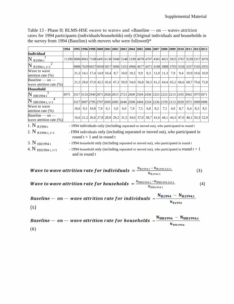
Table 13 - Phase II: RLMS-HSE «wave to wave» and «Baseline — on — wave» attrition
rates for 1994 participants (individuals/households) only (Original individuals and households in
the survey from 1994 (Baseline) with movers who were followed)*
1994 1995 1996 1998 2000 2001 2002 2003 2004 2005 2006 2007 2008 2009 2010 2011 2012 2013
Individual
N R1994 t1 11290 8886 8061 7108 6491 6138 5948 5548 5189 4878 4707 4381 4021 3925 3767 3539 3317 3076
N R1994 t, t+12 8886 7629 6657 6050 5817 5606 5353 4966 4677 4471 4188 3888 3703 3556 3357 3165 2955
Wave to wave
attrition rate (%) 21,3 14,1 17,4 14,9 10,4 8,7 10,0 10,5 9,9 8,3 11,0 11,3 7,9 9,4 10,9 10,6 10,9
Baseline — on —
wave attrition rate (%) 21,3 28,6 37,0 42,5 45,6 47,3 50,9 54,0 56,8 58,3 61,2 64,4 65,2 66,6 68,7 70,6 72,8
Household
N HH1994 t3 3975 3317 3133 2940 2871 2826 2815 2723 2600 2504 2436 2323 2223 2213 2105 2062 1975 1871
N HH1994 t, t+14
3317 3007 2795 2707 2695 2685 2646 2508 2404 2334 2236 2159 2113 2020 1971 1890 1808
Wave to wave
attrition rate (%) 16,6 9,3 10,8 7,9 6,1 5,0 6,0 7,9 7,5 6,8 8,2 7,1 4,9 8,7 6,4 8,3 8,5
Baseline — on —
wave attrition rate (%) 16,6 21,2 26,0 27,8 28,9 29,2 31,5 34,6 37,0 38,7 41,6 44,1 44,3 47,0 48,1 50,3 52,9
1. N R1994 t - 1994 individuals only (including separated or moved out), who participated in round t
2. N R1994 t, t+1 - 1994 individuals only (including separated or moved out), who participated in
round t + 1 and in round t
3. N HH1994 t - 1994 household only (including separated or moved out), who participated in round t
4. N HH1994 t, t+1 - 1994 household only (including separated or moved out), who participated in round t + 1
and in round t
𝑾𝒂𝒗𝒆 𝒕𝒐 𝒘𝒂𝒗𝒆 𝒂𝒕𝒕𝒓𝒊𝒕𝒊𝒐𝒏 𝒓𝒂𝒕𝒆 𝒇𝒐𝒓 𝒊𝒏𝒅𝒊𝒗𝒊𝒅𝒖𝒂𝒍𝒔 = NR1994 t − NR1994 t,t+1
NR1994 t (3)
𝑾𝒂𝒗𝒆 𝒕𝒐 𝒘𝒂𝒗𝒆 𝒂𝒕𝒕𝒓𝒊𝒕𝒊𝒐𝒏 𝒓𝒂𝒕𝒆 𝒇𝒐𝒓 𝒉𝒐𝒖𝒔𝒆𝒉𝒐𝒍𝒅𝒔 =NHH1994 t −NHH1994 t,t+1
NHH1994 t (4)
(5)
(6)
Supplemental Material
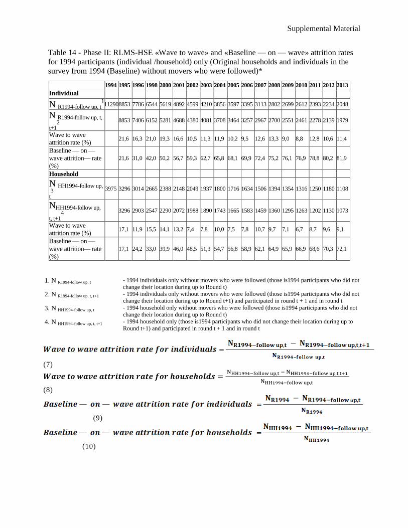
Table 14 - Phase II: RLMS-HSE «Wave to wave» and «Baseline — on — wave» attrition rates
for 1994 participants (individual /household) only (Original households and individuals in the
survey from 1994 (Baseline) without movers who were followed)*
1994 1995 1996 1998 2000 2001 2002 2003 2004 2005 2006 2007 2008 2009 2010 2011 2012 2013
Individual
N R1994-follow up, t1 11290 8853 7786 6544 5619 4892 4599 4210 3856 3597 3395 3113 2802 2699 2612 2393 2234 2048
N R1994-follow up, t,
t+12 8853 7406 6152 5281 4688 4380 4081 3708 3464 3257 2967 2700 2551 2461 2278 2139 1979
Wave to wave
attrition rate (%) 21,6 16,3 21,0 19,3 16,6 10,5 11,3 11,9 10,2 9,5 12,6 13,3 9,0 8,8 12,8 10,6 11,4
Baseline — on —
wave attrition–– rate
(%)
21,6 31,0 42,0 50,2 56,7 59,3 62,7 65,8 68,1 69,9 72,4 75,2 76,1 76,9 78,8 80,2 81,9
Household
N HH1994-follow up,
t3
3975 3296 3014 2665 2388 2148 2049 1937 1800 1716 1634 1506 1394 1354 1316 1250 1180 1108
NHH1994-follow up,
t, t+14
3296 2903 2547 2290 2072 1988 1890 1743 1665 1583 1459 1360 1295 1263 1202 1130 1073
Wave to wave
attrition rate (%) 17,1 11,9 15,5 14,1 13,2 7,4 7,8 10,0 7,5 7,8 10,7 9,7 7,1 6,7 8,7 9,6 9,1
Baseline — on —
wave attrition–– rate
(%)
17,1 24,2 33,0 39,9 46,0 48,5 51,3 54,7 56,8 58,9 62,1 64,9 65,9 66,9 68,6 70,3 72,1
1. N R1994-follow up, t - 1994 individuals only without movers who were followed (those is1994 participants who did not
change their location during up to Round t)
2. N R1994-follow up, t, t+1 - 1994 individuals only without movers who were followed (those is1994 participants who did not
change their location during up to Round t+1) and participated in round t + 1 and in round t
3. N HH1994-follow up, t - 1994 household only without movers who were followed (those is1994 participants who did not
change their location during up to Round t)
4. N HH1994-follow up, t, t+1 - 1994 household only (those is1994 participants who did not change their location during up to
Round t+1) and participated in round t + 1 and in round t
(7)
𝑾𝒂𝒗𝒆 𝒕𝒐 𝒘𝒂𝒗𝒆 𝒂𝒕𝒕𝒓𝒊𝒕𝒊𝒐𝒏 𝒓𝒂𝒕𝒆 𝒇𝒐𝒓 𝒉𝒐𝒖𝒔𝒆𝒉𝒐𝒍𝒅𝒔 = NHH1994−follow up,t − NHH1994−follow up,t,t+1
NHH1994−follow up,t
(8)
(9)
(10)