Data preprocessing D BM G Data Base and Data Mining Group ...

Data Base and Data Mining Group of Politecnico di Torino

DBMG

Data preprocessing

Elena Baralis, Tania CerquitelliPolitecnico di Torino

2DBMG

Outline

◼ Data types and properties

◼ Data preparation

◼ Data preparation for document data

◼ Similarity and dissimilarity

◼ Correlation


DBMG

Data types and properties

4DBMG

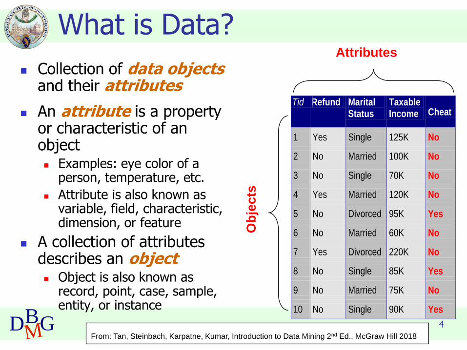
What is Data?

◼ Collection of data objects and their attributes

◼ An attribute is a property or characteristic of an object◼ Examples: eye color of a

person, temperature, etc.

◼ Attribute is also known as variable, field, characteristic, dimension, or feature

◼ A collection of attributes describes an object◼ Object is also known as

record, point, case, sample, entity, or instance

Tid Refund Marital Status

Taxable Income Cheat

1 Yes Single 125K No

2 No Married 100K No

3 No Single 70K No

4 Yes Married 120K No

5 No Divorced 95K Yes

6 No Married 60K No

7 Yes Divorced 220K No

8 No Single 85K Yes

9 No Married 75K No

10 No Single 90K Yes 10

Attributes

Ob

jec

ts

From: Tan, Steinbach, Karpatne, Kumar, Introduction to Data Mining 2nd Ed., McGraw Hill 2018

5DBMG

Attribute Values◼ Attribute values are numbers or symbols

assigned to an attribute for a particular object

◼ Distinction between attributes and attribute values◼ Same attribute can be mapped to different

attribute values◼ Example: height can be measured in feet or meters

◼ Different attributes can be mapped to the same set of values◼ Example: Attribute values for ID and age are integers

◼ But properties of attribute values can be different


6DBMG

Attribute types

◼ There are different types of attributes

◼ Nominal

◼ Examples: ID numbers, eye color, zip codes

◼ Ordinal

◼ Examples: rankings (e.g., taste of potato chips on a scale from 1-10), grades, height in {tall, medium, short}

◼ Interval

◼ Examples: calendar dates

◼ Ratio

◼ Examples: temperature in Kelvin, length, time, counts

From: Tan,Steinbach, Kumar, Introduction to Data Mining, McGraw Hill 2006

7DBMG

Properties of Attribute Values

◼ The type of an attribute depends on which of the following properties it possesses:

◼ Distinctness: =

◼ Order: < >

◼ Addition: + -

◼ Multiplication: * /

◼ Nominal attribute: distinctness

◼ Ordinal attribute: distinctness & order

◼ Interval attribute: distinctness, order & addition

◼ Ratio attribute: all 4 properties


8DBMG

Discrete and Continuous Attributes

◼ Discrete Attribute◼ Has only a finite or countably infinite set of values

◼ Examples: zip codes, counts, or the set of words in a collection of documents

◼ Often represented as integer variables.

◼ Note: binary attributes are a special case of discrete attributes

◼ Continuous Attribute◼ Has real numbers as attribute values

◼ Examples: temperature, height, or weight.

◼ Practically, real values can only be measured and represented using a finite number of digits.

◼ Continuous attributes are typically represented as floating-point variables.


9DBMG

More Complicated Examples

◼ ID numbers

◼ Nominal, ordinal, or interval?

◼ Number of cylinders in an automobile engine

◼ Nominal, ordinal, or ratio?


10DBMG

Key Messages for Attribute Types

◼ The types of operations you choose should be “meaningful” for the type of data you have◼ Distinctness, order, meaningful intervals, and meaningful ratios

are only four properties of data

◼ The data type you see – often numbers or strings – may not capture all the properties or may suggest properties that are not there

◼ Analysis may depend on these other properties of the data◼ Many statistical analyses depend only on the distribution

◼ Many times what is meaningful is measured by statistical significance

◼ But in the end, what is meaningful is measured by the domain


11DBMG

Data set types◼ Record

◼ Tables

◼ Document Data

◼ Transaction Data

◼ Graph

◼ World Wide Web

◼ Molecular Structures

◼ Ordered◼ Spatial Data

◼ Temporal Data

◼ Sequential Data

◼ Genetic Sequence Data


12DBMG

Tabular Data

◼ A collection of records

◼ Each record is characterized by a fixed set of attributes Tid Refund Marital

Status Taxable Income Cheat

1 Yes Single 125K No

2 No Married 100K No

3 No Single 70K No

4 Yes Married 120K No

5 No Divorced 95K Yes

6 No Married 60K No

7 Yes Divorced 220K No

8 No Single 85K Yes

9 No Married 75K No

10 No Single 90K Yes 10


13DBMG

◼ It includes textual data that can be semi-structured or unstructured

◼ Plain text can be organized in sentences, paragraphs,sections, documents

◼ Text acquired in different contexts may have astructure and/or a semantics

◼ Web pages are enriched with tags

◼ Documents in digital libraries are enriched withmetadata

◼ E-learning documents can be annotated or partlyhighglihted

Document data

14DBMG

Transaction Data

◼ A special type of record data, where

◼ each record (transaction) involves a set of items.

◼ For example, consider a grocery store. The set of products purchased by a customer during one shopping trip constitute a transaction, while the individual products that were purchased are the items.

TID Items

1 Bread, Coke, Milk

2 Beer, Bread

3 Beer, Coke, Diaper, Milk

4 Beer, Bread, Diaper, Milk

5 Coke, Diaper, Milk


15DBMG

Graph Data

◼ Examples: Generic graph, a molecule, and webpages

5

2

1

2

5

Benzene Molecule: C6H6


16DBMG

Ordered Data

◼ Sequences of transactions

An element of the sequence

Items/Events


17DBMG

Ordered Data

◼ Genomic sequence data

GGTTCCGCCTTCAGCCCCGCGCC

CGCAGGGCCCGCCCCGCGCCGTC

GAGAAGGGCCCGCCTGGCGGGCG

GGGGGAGGCGGGGCCGCCCGAGC

CCAACCGAGTCCGACCAGGTGCC

CCCTCTGCTCGGCCTAGACCTGA

GCTCATTAGGCGGCAGCGGACAG

GCCAAGTAGAACACGCGAAGCGC

TGGGCTGCCTGCTGCGACCAGGG


18DBMG

Ordered Data

◼ Spatio-Temporal Data

Average Monthly Temperature of land and ocean


19DBMG

Data Quality ◼ Poor data quality negatively affects many data processing

efforts

“The most important point is that poor data quality is an unfolding

disaster. Poor data quality costs the typical company at least ten percent (10%) of revenue; twenty percent (20%) is probably a better estimate.”

Thomas C. Redman, DM Review, August 2004

◼ Data mining example: a classification model for detecting people who are loan risks is built using poor data

◼ Some credit-worthy candidates are denied loans

◼ More loans are given to individuals that default


20DBMG

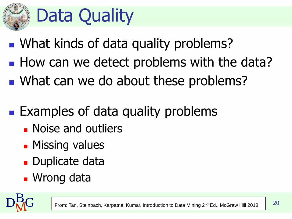
Data Quality

◼ What kinds of data quality problems?

◼ How can we detect problems with the data?

◼ What can we do about these problems?

◼ Examples of data quality problems

◼ Noise and outliers

◼ Missing values

◼ Duplicate data

◼ Wrong data


21DBMG

Noise

◼ Noise refers to modification of original values

◼ Examples: distortion of a person’s voice when talking on a poor phone and “snow” on television screen

Two Sine Waves Two Sine Waves + Noise


22DBMG

◼ Outliers are data objects with characteristics that are considerably different than most of the other data objects in the data set

◼ Case 1: Outliers are noise that interfereswith data analysis

◼ Case 2: Outliers are the goal of our analysis

◼ Credit card fraud

◼ Intrusion detection

Outliers


23DBMG

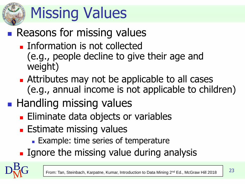
Missing Values◼ Reasons for missing values

◼ Information is not collected (e.g., people decline to give their age and weight)

◼ Attributes may not be applicable to all cases (e.g., annual income is not applicable to children)

◼ Handling missing values◼ Eliminate data objects or variables

◼ Estimate missing values◼ Example: time series of temperature

◼ Ignore the missing value during analysis


24DBMG

Duplicate Data

◼ Data set may include data objects that are duplicates, or almost duplicates of one another◼ Major issue when merging data from heterogeneous

sources

◼ Examples:◼ Different words/abbreviations for the same concept (e.g.,

Street, St.)

◼ Data cleaning◼ Process of dealing with duplicate data issues

◼ When should duplicate data not be removed?



DBMG

Data preparation

26DBMG

Data Preprocessing

◼ Aggregation

◼ Sampling

◼ Dimensionality Reduction

◼ Feature subset selection

◼ Feature creation

◼ Discretization and Binarization

◼ Attribute Transformation


27DBMG

Aggregation

◼ Combining two or more attributes (or objects) into a single attribute (or object)

◼ Purpose

◼ Data reduction

◼ Reduce the number of attributes or objects

◼ Change of scale

◼ Cities aggregated into regions, states, countries, etc

◼ More “stable” data

◼ Aggregated data tends to have less variability


28DBMG

Aggregation

Standard Deviation of Average Monthly Precipitation

Standard Deviation of Average Yearly Precipitation

Variation of Precipitation in Australia


29DBMG

Example: Precipitation in Australia

◼ The previous slide shows precipitation in Australia from the period 1982 to 1993

◼ A histogram for the standard deviation of average monthly precipitation for 3,030 0.5◦ by 0.5◦ grid cells in Australia, and

◼ A histogram for the standard deviation of the average yearly precipitation for the same locations.

◼ The average yearly precipitation has less variability than the average monthly precipitation.

◼ All precipitation measurements (and their standard deviations) are in centimeters.


30DBMG

Data reduction

◼ It generates a reduced representation of the dataset. This representation is smaller in volume, but it can provide similar analytical results

◼ sampling

◼ It reduces the cardinality of the set

◼ feature selection

◼ It reduces the number of attributes

◼ discretization

◼ It reduces the cardinality of the attribute domain

31DBMG

Sampling

◼ Sampling is the main technique employed for dataselection.◼ It is often used for both the preliminary investigation

of the data and the final data analysis.

◼ Statisticians sample because obtaining the entireset of data of interest is too expensive or timeconsuming.

◼ Sampling is used in data mining becauseprocessing the entire set of data of interest is tooexpensive or time consuming.


32DBMG

Sampling …

◼ The key principle for effective sampling is the following:

◼ using a sample will work almost as well as using the entire data set, if the sample is representative

◼ A sample is representative if it has approximately the same property (of interest) as the original set of data


33DBMG

Sample Size: examples

8000 points 2000 Points 500 Points


34DBMG

Types of Sampling◼ Simple Random Sampling

◼ There is an equal probability of selecting any particular item

◼ Sampling without replacement◼ As each item is selected, it is removed from the

population

◼ Sampling with replacement◼ Objects are not removed from the population as they are

selected for the sample.

◼ In sampling with replacement, the same object can be picked up more than once

◼ Stratified sampling◼ Split the data into several partitions; then draw

random samples from each partition


35DBMG

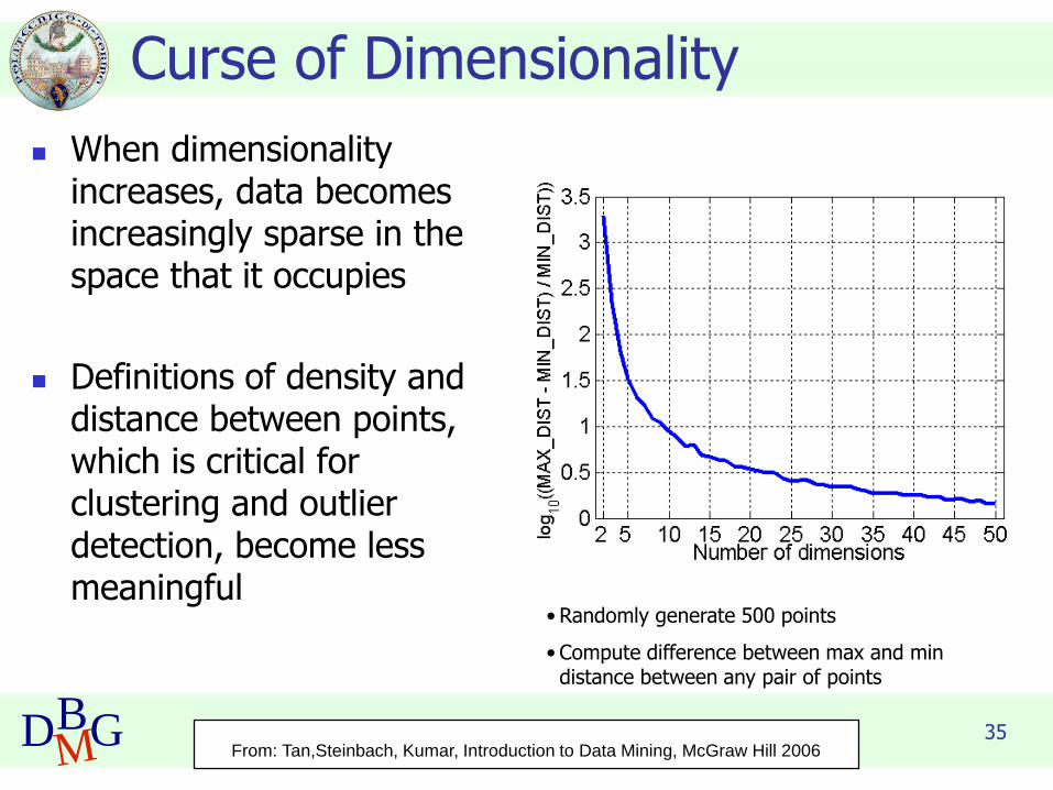
Curse of Dimensionality

◼ When dimensionality increases, data becomes increasingly sparse in the space that it occupies

◼ Definitions of density and distance between points, which is critical for clustering and outlier detection, become less meaningful

• Randomly generate 500 points

• Compute difference between max and min distance between any pair of points


36DBMG

Dimensionality Reduction

◼ Purpose◼ Avoid curse of dimensionality

◼ Reduce amount of time and memory required by data mining algorithms

◼ Allow data to be more easily visualized

◼ May help to eliminate irrelevant features or reduce noise

◼ Techniques◼ Principal Component Analysis (PCA)

◼ Singular Value Decomposition

◼ Others: supervised and non-linear techniques


37DBMG

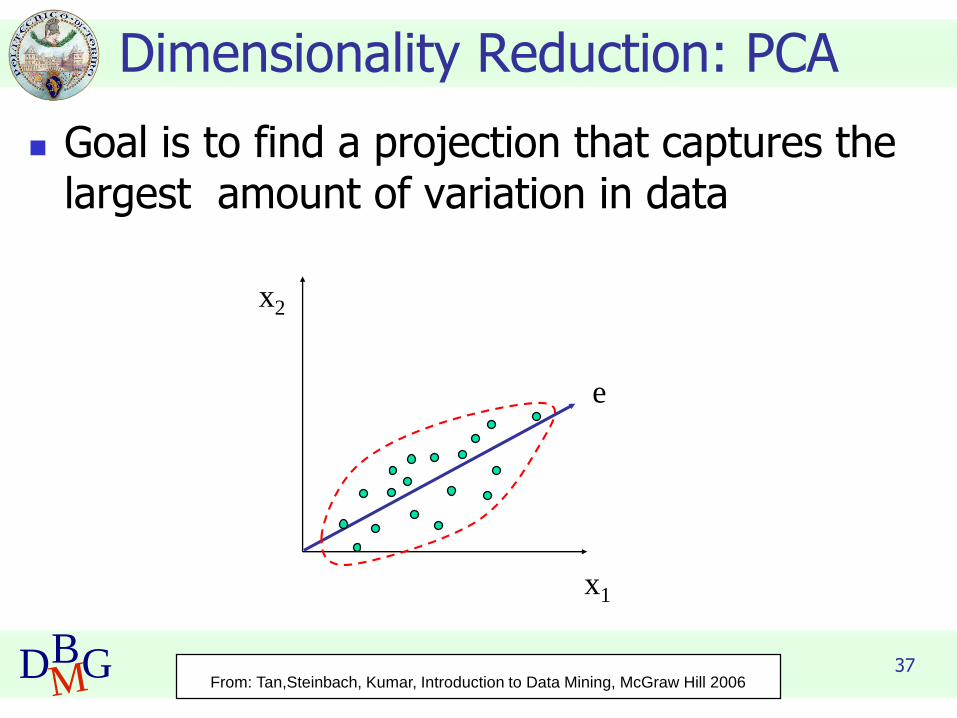
Dimensionality Reduction: PCA

◼ Goal is to find a projection that captures the largest amount of variation in data

x2

x1

e


38DBMG

Dimensionality Reduction: PCA


39DBMG

Feature Subset Selection

◼ Another way to reduce dimensionality of data

◼ Redundant features ◼ duplicate much or all of the information contained in one

or more other attributes

◼ Example: purchase price of a product and the amount of sales tax paid

◼ Irrelevant features◼ contain no information that is useful for the data mining

task at hand

◼ Example: students' ID is often irrelevant to the task of predicting students' GPA


40DBMG

Feature Subset Selection

◼ Techniques

◼ Brute-force approach

◼ Try all possible feature subsets as input to data mining algorithm

◼ Embedded approaches

◼ Feature selection occurs naturally as part of the data mining algorithm

◼ Filter approaches

◼ Features are selected before data mining algorithm is run

◼ Wrapper approaches

◼ Use the data mining algorithm as a black-box to find best subset of attributes


41DBMG

Feature Creation

◼ Create new attributes that can capture the important information in a data set much more efficiently than the original attributes

◼ Three general methodologies

◼ Feature Extraction

◼ domain-specific

◼ Mapping Data to New Space

◼ Feature Construction

◼ combining features


42DBMG

Mapping Data to a New Space

Two Sine Waves Two Sine Waves + Noise Frequency

Fourier transform

Wavelet transform


43DBMG

Discretization

◼ Discretization is the process of converting a continuous attribute into an ordinal attribute

◼ A potentially infinite number of values are mapped into a small number of categories

◼ Discretization is commonly used in classification

◼ Many classification algorithms work best if both the independent and dependent variables have only a few values


44DBMG

Virginica. Robert H. Mohlenbrock. USDA NRCS. 1995.

Northeast wetland flora: Field office guide to plant

species. Northeast National Technical Center, Chester,

PA. Courtesy of USDA NRCS Wetland Science Institute.

Iris Sample Data Set

◼ Iris Plant data set◼ Can be obtained from the UCI Machine Learning Repository

http://www.ics.uci.edu/~mlearn/MLRepository.html

◼ From the statistician Douglas Fisher

◼ Three flower types (classes)◼ Setosa

◼ Versicolour

◼ Virginica

◼ Four (non-class) attributes◼ Sepal width and length

◼ Petal width and length


http://www.ics.uci.edu/~mlearn/MLRepository.html

45DBMG

Discretization: Iris Example

Petal width low or petal length low implies Setosa.Petal width medium or petal length medium implies Versicolour.Petal width high or petal length high implies Virginica.


46DBMG

Discretization: Iris Example …

◼ How can we tell what the best discretization is?◼ Unsupervised discretization: find breaks in the

data values◼ Example:

Petal Length

◼ Supervised discretization: Use class labels to find breaks

0 2 4 6 80

10

20

30

40

50

Petal Length

Counts


47DBMG

Discretization

◼ Examples of unsupervised discretization techniques◼ N intervals with the same width W=(vmax – vmin)/N

◼ Easy to implement

◼ It can be badly affected by outliers and sparse data

◼ Incremental approach

◼ N intervals with (approximately) the same cardinality◼ It better fits sparse data and outliers

◼ Non incremental approach

◼ clustering◼ It fits well sparse data and outliers

◼ analysis of data distribution◼ e.g., 4 intervals, one for each quartile

48DBMG

Example: unsupervised discretization technique

Data consists of four groups of points and two outliers. Data is one-

dimensional, but a random y component is added to reduce overlap.


49DBMG

Equal interval width approach used to obtain 4 values.



50DBMG

Equal frequency approach used to obtain 4 values.



51DBMG

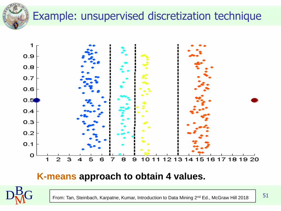
K-means approach to obtain 4 values.



52DBMG

Binarization

◼ Binarization maps an attribute into one or more binary variables

◼ Continuous attribute: first map the attribute to a categorical one ◼ Example: height measured as {low, medium, high}

◼ Categorical attribute◼ Mapping to a set of binary attributes

◼ Example: Low, medium, high as 1 0 0, 0 1 0, 0 0 1

53DBMG

Attribute Transformation

◼ An attribute transform is a function that maps the entire set of values of a given attribute to a new set of replacement values such that each old value can be identified with one of the new values◼ Simple functions: xk, log(x), ex, |x|

◼ Normalization

◼ Refers to various techniques to adjust to differences among attributes in terms of frequency of occurrence, mean, variance, range

◼ Take out unwanted, common signal, e.g., seasonality

◼ In statistics, standardization refers to subtracting off the means and dividing by the standard deviation


54DBMG

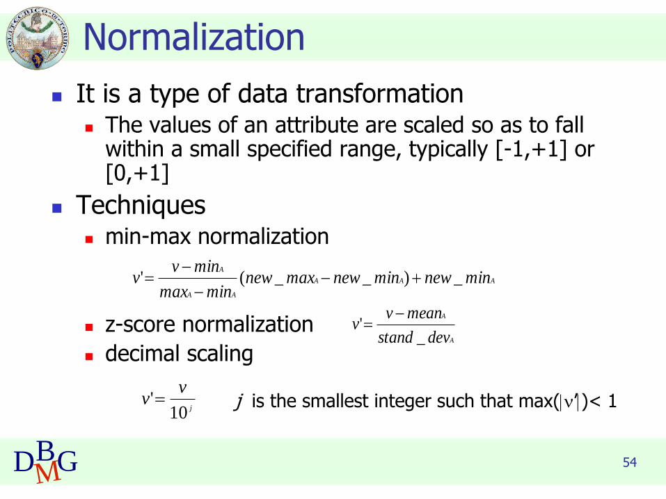
Normalization

◼ It is a type of data transformation◼ The values of an attribute are scaled so as to fall

within a small specified range, typically [-1,+1] or [0,+1]

◼ Techniques◼ min-max normalization

◼ z-score normalization

◼ decimal scaling

AAA

AA

A

minnewminnewmaxnewminmax

minvv _)__(' +−

−

−=

A

A

devstand

meanvv

_'

−=

j

vv

10'= j is the smallest integer such that max(’)< 1

55DBMG

Example: Sample Time Series of Plant Growth

Correlations between time series

Minneapolis

Minneapolis Atlanta Sao Paolo

Minneapolis 1.0000 0.7591 -0.7581

Atlanta 0.7591 1.0000 -0.5739

Sao Paolo -0.7581 -0.5739 1.0000


Net Primary

Production (NPP)

is a measure of

plant growth used

by ecosystem

scientists.


56DBMG


Minneapolis

Normalized using monthly Z Score:

Subtract off monthly mean and divide by monthly standard deviation

Minneapolis Atlanta Sao Paolo

Minneapolis 1.0000 0.0492 0.0906

Atlanta 0.0492 1.0000 -0.0154

Sao Paolo 0.0906 -0.0154 1.0000



Example: Sample Time Series of Plant Growth


DBMG

Data preparation for document data

58DBMG

◼ A document might be modeled in different ways

◼ The choice heavily affects the quality of the miningresult

◼ The most common representation models adocument as a set of features

◼ Each feature might represent a set of characters, aword, a term, a concept

Document representation

59DBMG

◼ It is the activity to generate a structureddata representation of document data

◼ It includes five sequential steps

◼ Document splitting

◼ Tokenisation

◼ Case normalisation

◼ Stopword removal

◼ Stemming

Document processing

60DBMG

◼ Based on the data analytics goal documents canbe split into

◼ sentences, paragraphs, or analyzed in their entirecontent

◼ Short documents are typically not split

◼ e.g., emails or social posts

◼ Long documents can be

◼ broken up into sections or paragraphs

◼ analyzed as a whole

Document splitting

61DBMG

◼ It is the process of breaking text into sentencesor text into tokens (i.e., words)

◼ Identify sentence boundaries based on punctuation,capitalization

◼ Separate words in sentences

◼ Language-dependent

Tokenization

62DBMG

◼ This step converts each token to completelyupper-case or lower-case characters

◼ Capitalisation helps human readers differentiate, forexample, between nouns and proper nouns and canbe useful for automated algorithms as well

◼ However, an upper-case word at the beginning ofthe sentence should be treated no differently thanthe same word in lower case appearing elsewhere ina document

Case normalization

63DBMG

◼ Reduce a word to its root form (i.e., the stem)

◼ It includes the identification and removal of prefixes,suffixes, and pluralisation

◼ It operates on a single word without knowledge ofthe context

◼ It cannot discriminate between words which havedifferent meanings depending on the part of speech

◼ Stemmers are

◼ Easy to implement

◼ Available for most spoken languages

◼ Run significantly faster than lemmatization and POStagging algorithms

Stemming

64DBMG

◼ “Stop words” refers to the most common words in alanguage

◼ E.g., prepositions, articles, conjunctions in English

◼ Stop words are filtered out before or after processing oftextual data

◼ They are likely to have little semantic meaning

Stopword elimination

65DBMG

◼ There is no single universal list of stop words used byall natural language processing tools

◼ Any group of words can be chosen as the stop wordsfor a given purpose

◼ different search engines use different stop word lists

◼ Some of them remove lexical words, such as "want”, from aquery in order to improve performance

◼ Some tools specifically avoid removing these stop wordsto support phrase search

Stopword elimination


DBMG

Weighted documentrepresentation

67DBMG

◼ Most data mining algorithm are unable to directlyprocess textual data in their original form

◼ documents are transformed into a more manageablerepresentation

◼ Documents are represented by feature vectors

◼ A feature is simply an entity without internal structure

◼ A dimension of the feature space

◼ A document is represented as a vector in this space

◼ a collection of features and their weights

Text representation: feature vectors

68DBMG

Example

◼ Each document becomes a term vector

◼ each term is a component (attribute) of the vector

◼ the value of each component is the number of times the corresponding term occurs in the document

Document 1

se

aso

n

time

ou

t

lost

wi

n

ga

me

sco

re

ba

ll

play

co

ach

tea

m

Document 2

Document 3

3 0 5 0 2 6 0 2 0 2

0

0

7 0 2 1 0 0 3 0 0

1 0 0 1 2 2 0 3 0


69DBMG

◼ All words in a document are considered as separatefeatures

◼ the dimension of the feature space is equal to the number ofdifferent words in all of the documents

◼ The feature vector of a document consists of a set ofweights, one for each distinct word

◼ The methods of giving weights to the features may vary

Bag-of-word representation

70DBMG

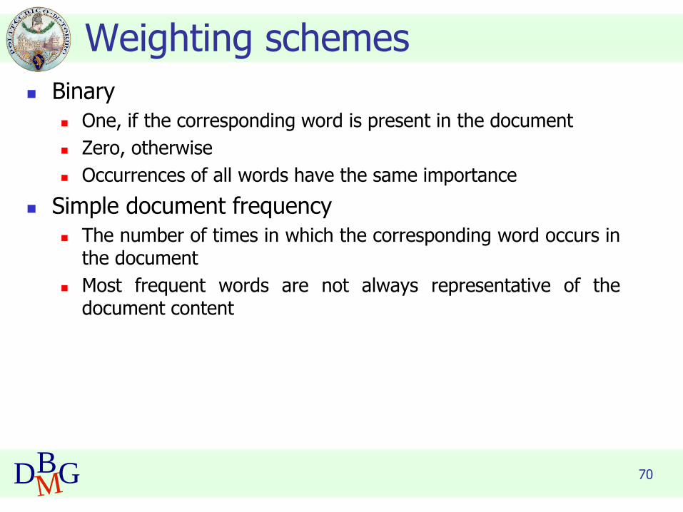
◼ Binary

◼ One, if the corresponding word is present in the document

◼ Zero, otherwise

◼ Occurrences of all words have the same importance

◼ Simple document frequency

◼ The number of times in which the corresponding word occurs inthe document

◼ Most frequent words are not always representative of thedocument content

Weighting schemes

71DBMG

◼ More complex weighting schemes are possible to takeinto account the frequency of the word

◼ in the document

◼ in the section/paragraph

◼ in the category (for indexed documents)

◼ in the collection of documents

Weighting schemes

72DBMG

Weighting schemes

◼ Term frequency inverse document frequency (tf-idf)◼ Tf-idf of term t in document d of collection D (consisting of m

documents)

tf-idf(t) = freq(t, d) * log(m/freq(t, D))

◼ Terms occurring frequently in a single document but rarely in thewhole collection are preferred

◼ Suitable for

◼ A single document consisting of many sections orsubsections

◼ A collection of heterogeneous documents

73DBMG

Weighting schemes

◼ Term frequency document frequency (tf-df)◼ Tf-df of term t in document d of collection D

tf-df(t) = freq(t, d) * log(freq(t, D))

◼ Terms occurring frequently both in a single document and in thewhole collection are preferred

◼ Suitable for

◼ Single documents or parts of a document withhomogeneous content

◼ A collection of documents ranging over the sametopic

74DBMG

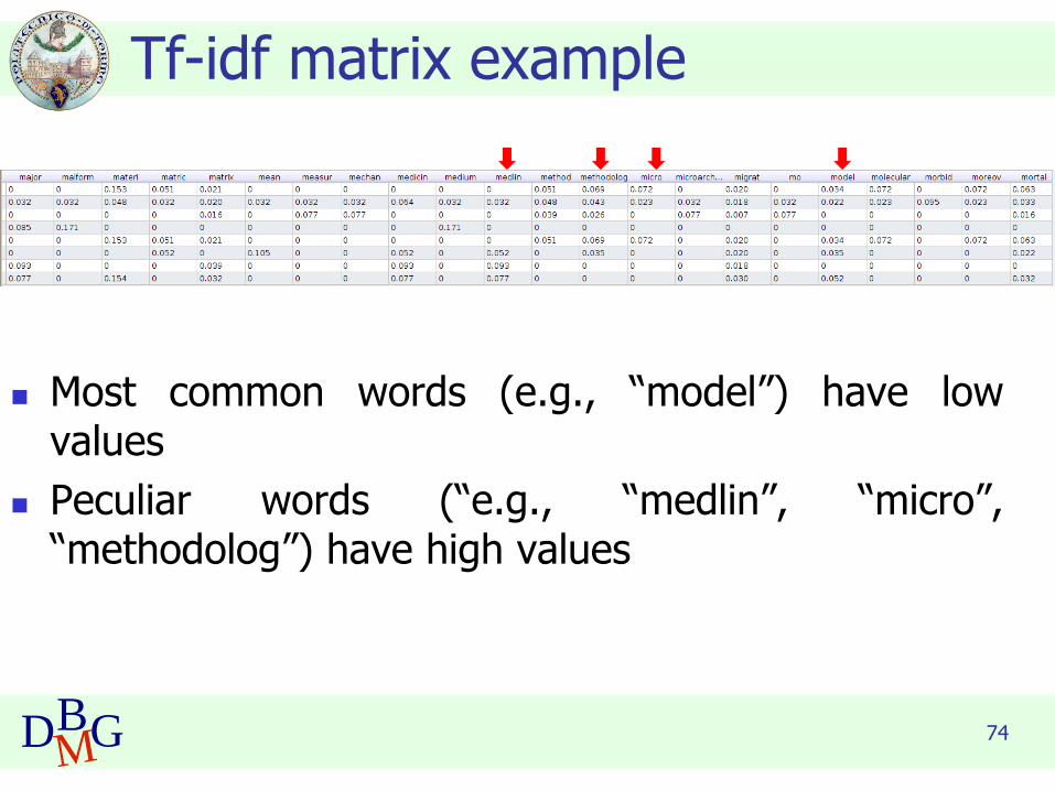
Tf-idf matrix example

◼ Most common words (e.g., “model”) have lowvalues

◼ Peculiar words (“e.g., “medlin”, “micro”,“methodolog”) have high values

75DBMG

Weighting schemes

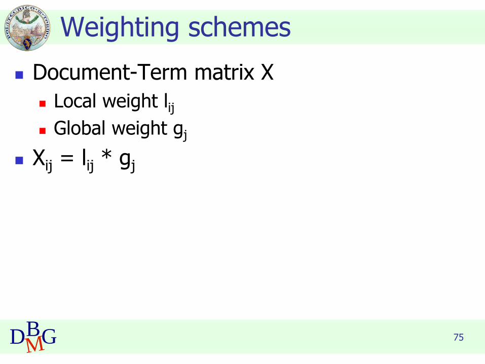
◼ Document-Term matrix X

◼ Local weight lij◼ Global weight gj

◼ Xij = lij * gj


DBMG

Similarity and dissimilarity

77DBMG

Similarity and Dissimilarity

◼ Similarity

◼ Numerical measure of how alike two data objects are

◼ Is higher when objects are more alike

◼ Often falls in the range [0,1]

◼ Dissimilarity

◼ Numerical measure of how different are two data objects

◼ Lower when objects are more alike

◼ Minimum dissimilarity is often 0

◼ Upper limit varies

◼ Proximity refers to a similarity or dissimilarity


78DBMG

Similarity/Dissimilarity for Simple Attributes

The following table shows the similarity and dissimilarity

between two objects, x and y, with respect to a single, simple

attribute.


79DBMG

Euclidean Distance

◼ Euclidean Distance

where n is the number of dimensions (attributes) and xk and yk are, respectively, the kth attributes (components) of data objects xand y.

Standardization is necessary, if scales differ.


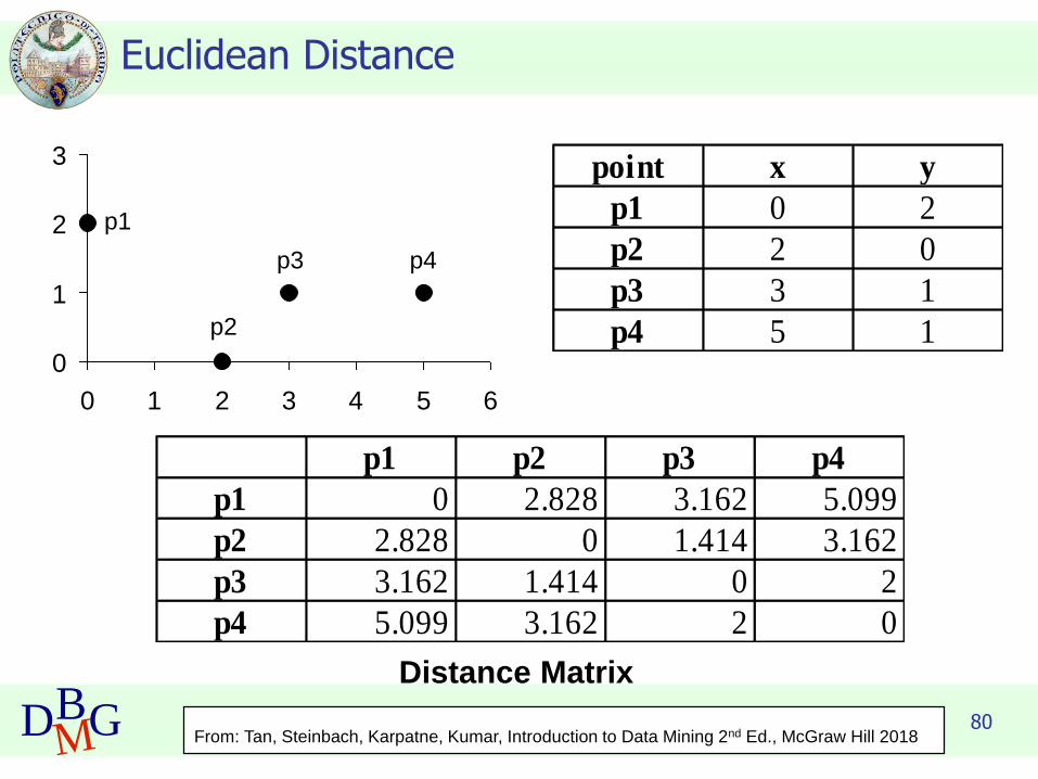
80DBMG

Euclidean Distance

0

1

2

3

0 1 2 3 4 5 6

p1

p2

p3 p4

point x y

p1 0 2

p2 2 0

p3 3 1

p4 5 1

Distance Matrix

p1 p2 p3 p4

p1 0 2.828 3.162 5.099

p2 2.828 0 1.414 3.162

p3 3.162 1.414 0 2

p4 5.099 3.162 2 0


81DBMG

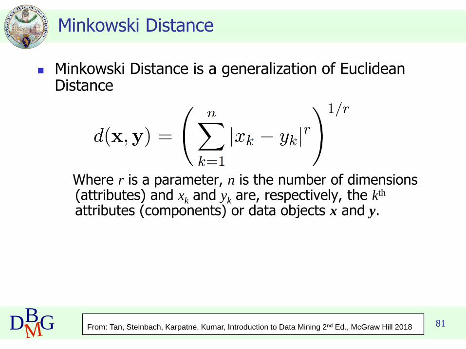
Minkowski Distance

◼ Minkowski Distance is a generalization of Euclidean Distance

Where r is a parameter, n is the number of dimensions (attributes) and xk and yk are, respectively, the kth

attributes (components) or data objects x and y.


82DBMG

Minkowski Distance: Examples

◼ r = 1. City block (Manhattan, taxicab, L1 norm) distance.

◼ A common example of this is the Hamming distance, which is just the number of bits that are different between two binary vectors

◼ r = 2. Euclidean distance

◼ r → . “supremum” (Lmax norm, L norm) distance.

◼ This is the maximum difference between any component of the vectors

◼ Do not confuse r with n, i.e., all these distances are defined for all numbers of dimensions.


83DBMG

Minkowski Distance

Distance Matrix

point x y

p1 0 2

p2 2 0

p3 3 1

p4 5 1

L1 p1 p2 p3 p4

p1 0 4 4 6

p2 4 0 2 4

p3 4 2 0 2

p4 6 4 2 0

L2 p1 p2 p3 p4

p1 0 2.828 3.162 5.099

p2 2.828 0 1.414 3.162

p3 3.162 1.414 0 2

p4 5.099 3.162 2 0

L p1 p2 p3 p4

p1 0 2 3 5

p2 2 0 1 3

p3 3 1 0 2

p4 5 3 2 0


84DBMG

Mahalanobis Distance

For red points, the Euclidean distance is 14.7, Mahalanobis distance is 6.

is the covariance matrix

𝐦𝐚𝐡𝐚𝐥𝐚𝐧𝐨𝐛𝐢𝐬 𝐱, 𝐲 = (𝐱 − 𝐲)𝑇 Ʃ−1(𝐱 − 𝐲)


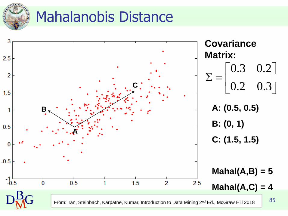
85DBMG

Mahalanobis Distance

Covariance

Matrix:

=

3.02.0

2.03.0

A: (0.5, 0.5)

B: (0, 1)

C: (1.5, 1.5)

Mahal(A,B) = 5

Mahal(A,C) = 4

B

A

C


86DBMG

Common Properties of a Distance

◼ Distances, such as the Euclidean distance, have some well-known properties.

1. d(x, y) 0 for all x and y and d(x, y) = 0 only if x = y. (Positive definiteness)

2. d(x, y) = d(y, x) for all x and y. (Symmetry)3. d(x, z) d(x, y) + d(y, z) for all points x, y, and z.

(Triangle Inequality)

where d(x, y) is the distance (dissimilarity) between points (data objects) x and y.

◼ A distance that satisfies these properties is a metric


87DBMG

Common Properties of a Similarity

◼ Similarities, also have some well known properties.

1. s(x, y) = 1 (or maximum similarity) only if x= y.

2. s(x, y) = s(y, x) for all x and y. (Symmetry)

where s(x, y) is the similarity between points (data objects), x and y.


88DBMG

Similarity Between Binary Vectors

◼ Common situation is that objects, p and q, have only binary attributes

◼ Compute similarities using the following quantitiesM01 = the number of attributes where p was 0 and q was 1M10 = the number of attributes where p was 1 and q was 0M00 = the number of attributes where p was 0 and q was 0M11 = the number of attributes where p was 1 and q was 1

◼ Simple Matching and Jaccard Coefficients SMC = number of matches / number of attributes

= (M11 + M00) / (M01 + M10 + M11 + M00)

J = number of 11 matches / number of not-both-zero attributes values= (M11) / (M01 + M10 + M11)


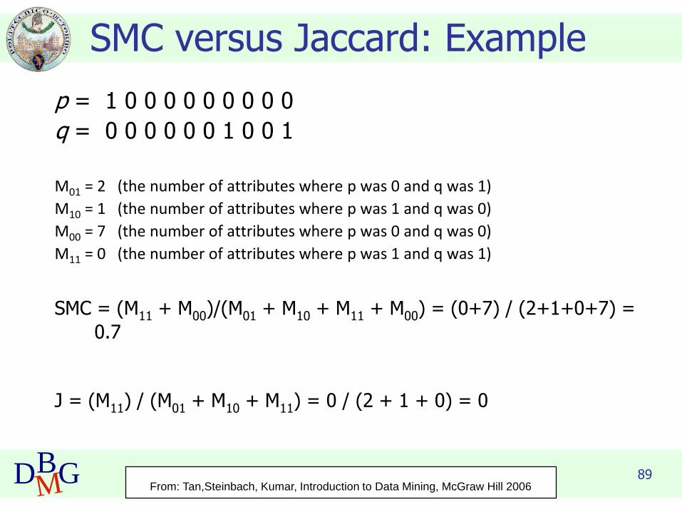
89DBMG

SMC versus Jaccard: Example

p = 1 0 0 0 0 0 0 0 0 0

q = 0 0 0 0 0 0 1 0 0 1

M01 = 2 (the number of attributes where p was 0 and q was 1)




SMC = (M11 + M00)/(M01 + M10 + M11 + M00) = (0+7) / (2+1+0+7) =

0.7

J = (M11) / (M01 + M10 + M11) = 0 / (2 + 1 + 0) = 0


90DBMG

Cosine Similarity

◼ If d1 and d2 are two document vectors, then

cos( d1, d2 ) = (d1 • d2) / ||d1|| ||d2|| ,

where • indicates vector dot product and || d || is the norm of vector d.

◼ Example:

d1 = 3 2 0 5 0 0 0 2 0 0

d2 = 1 0 0 0 0 0 0 1 0 2

d1 • d2= 3*1 + 2*0 + 0*0 + 5*0 + 0*0 + 0*0 + 0*0 + 2*1 + 0*0 + 0*2 = 5

||d1|| = (3*3+2*2+0*0+5*5+0*0+0*0+0*0+2*2+0*0+0*0)0.5 = (42) 0.5 = 6.481

||d2|| = (1*1+0*0+0*0+0*0+0*0+0*0+0*0+1*1+0*0+2*2) 0.5 = (6) 0.5 = 2.245

cos( d1, d2 ) = .3150


91DBMG

General Approach for Combining Similarities

◼ Sometimes attributes are of many different types, but an overall similarity is needed.

1: For the kth attribute, compute a similarity, sk(x, y), in the

range [0, 1].

2: Define an indicator variable, k, for the kth attribute as

follows:

k = 0 if the kth attribute is an asymmetric attribute and

both objects have a value of 0, or if one of the objects has a missing value for the kth attribute

k = 1 otherwise

3. Compute


92DBMG

Using Weights to Combine Similarities

◼ May not want to treat all attributes the same.

◼ Use non-negative weights 𝜔𝑘

◼ 𝑠𝑖𝑚𝑖𝑙𝑎𝑟𝑖𝑡𝑦 𝐱, 𝐲 =σ𝑘=1𝑛 𝜔𝑘𝛿𝑘𝑠𝑘(𝐱,𝐲)

σ𝑘=1𝑛 𝜔𝑘𝛿𝑘

◼ Can also define a weighted form of distance



DBMG

Correlation

94DBMG

Data correlation

◼ Measure of the linear relationship between two data objects

◼ having binary or continuous variables

◼ Useful during the data exploration phase

◼ To be better aware of data properties

◼ Analysis of feature correlation

◼ Correlated features should be removed

◼ simplifying the next analytics steps

◼ improving the performance of the data-driven algorithms

95DBMG

Pearson’s correlation


96DBMG

Visually Evaluating Correlation

Scatter plots showing the

similarity from –1 to 1.


Perfect linear correlation whenvalue is 1 or -1

97DBMG

Drawback of Correlation

◼ x = (-3, -2, -1, 0, 1, 2, 3)

◼ y = (9, 4, 1, 0, 1, 4, 9)

yi = xi2

◼ mean(x) = 0, mean(y) = 4

◼ std(x) = 2.16, std(y) = 3.74

corr = (-3)(5)+(-2)(0)+(-1)(-3)+(0)(-4)+(1)(-3)+(2)(0)+3(5) / ( 6 * 2.16 * 3.74 )

= 0


Data preprocessing D BM G Data Base and Data Mining Group ...

Documents

Transcript of Data preprocessing D BM G Data Base and Data Mining Group ...