Data mining of geospatial data:combining visual andautomatic methods

Urska Demsar

Doctoral thesis in Geoinformatics

Department of Urban Planning and EnvironmentSchool of Architecture and the Built Environment

Royal Institute of Technology (KTH)

Stockholm, April 2006

Akademisk avhandling som med tillstand av Kungliga Tekniska Hogskolan framlagges till offentliggranskning for avlaggande av teknologie doktorsexamen fredagen den 7 april 2006 kl. 10:00 ihorsalen F3, KTH, Lindstedtsvagen 26, Stockholm. Avhandlingen forsvaras pa engelska.

Urska Demsar, Data mining of geospatial data: combining visual and automatic methods

Supervisor:Doc. Hans Hauska,Urban Planning and Environment, School of Architecture and Built Environment, KTH,Stockholm, Sweden

Oponent:Prof. Peter A. Burrough,Oxford University Centre for Climate and Environment, OUCE, Oxford, UK

Evaluation committee:Prof. Kerstin Severinson Eklundh,NADA, School of Computer Science and Communication, KTH, Stockholm, SwedenProf. Erland Jungert,Department of Computer and Information Science, Linkopings University, Linkoping, SwedenDoc. Tiina Sarjakoski,Dept. of Geoinformatics and Cartography, Finnish Geodetic Institute, Helsinki, Finland

Copyright c© Urska Demsar, April 2006.

All rights reserved. No part of this thesis may be reproduced by any means without permis-sion from the author.

Paper II reprinted with permission of Presses Polytechniques et Universitaires Romandes.Paper III reprinted with permission of Dr. Fred Toppen and Dr. Poulicos Prastacos.Paper V reprinted with permission of Springer Verlag and Dr. Wolfgang Kainz.

Printed by Universitetsservice US-AB.Stockholm 2006

TRITA-SOM 06-01 • ISSN 1653-6126 • ISRN KTH/SOM/–06/001–SE • ISBN 91-7178-297-4

Abstract

Most of the largest databases currently available have a strong geospatialcomponent and contain potentially useful information which might be ofvalue. The discipline concerned with extracting this information and know-ledge is data mining. Knowledge discovery is performed by applying auto-matic algorithms which recognise patterns in the data.

Classical data mining algorithms assume that data are independentlygenerated and identically distributed. Geospatial data are multidimensional,spatially autocorrelated and heterogeneous. These properties make classicaldata mining algorithms inappropriate for geospatial data, as their basicassumptions cease to be valid. Extracting knowledge from geospatial datatherefore requires special approaches. One way to do that is to use visualdata mining, where the data is presented in visual form for a human toperform the pattern recognition. When visual mining is applied to geospatialdata, it is part of the discipline called exploratory geovisualisation.

Both automatic and visual data mining have their respective advantages.Computers can treat large amounts of data much faster than humans, whilehumans are able to recognise objects and visually explore data much moreeffectively than computers. A combination of visual and automatic datamining draws together human cognitive skills and computer efficiency andpermits faster and more efficient knowledge discovery.

This thesis investigates if a combination of visual and automatic datamining is useful for exploration of geospatial data. Three case studies il-lustrate three different combinations of methods. Hierarchical clustering iscombined with visual data mining for exploration of geographical metadatain the first case study. The second case study presents an attempt to ex-plore an environmental dataset by a combination of visual mining and aSelf-Organising Map. Spatial pre-processing and visual data mining me-thods were used in the third case study for emergency response data.

Contemporary system design methods involve user participation at allstages. These methods originated in the field of Human-Computer Interac-tion, but have been adapted for the geovisualisation issues related to spatialproblem solving. Attention to user-centred design was present in all threecase studies, but the principles were fully followed only for the third casestudy, where a usability assessment was performed using a combination ofa formal evaluation and exploratory usability.

Keywords: geovisualisation, spatial data mining, visual data mining, usability evaluation.

iii

Acknowledgements

I wish to thank my supervisor doc. Hans Hauska, who by accepting me asa PhD student gave me a chance to come to Stockholm and hopefully oneday become a scientist. I am grateful for all the support and guidance thathe has given me during my studies at KTH.

I would like to thank the co-authors of the papers that this thesis isbased upon for successfull cooperation in research and writing. MoreoverI am indebted to Kirlna Skeppstrom and Bo Olofsson from the Depart-ment for Land and Water Resources Engineering at KTH for cooperation incase study 2 and permission to use the radon dataset. I would also like toacknowledge the collaboration with Helsinki University of Technology andthank prof. Kirsi Virrantaus, Jukka Krisp and Olga Kremenova for collab-oration in case study 3 and for permission to use the emergency responsedataset and the jointly developed data mining system for the usability ex-periment that I performed.

Research presented in the first part of this thesis was conducted in theperiod 2002-2003 as a part of the project INVISIP (IST 2000-29640), whichwas financially supported by European Commission. The second part of thethesis would not be possible without financial support from the Municipalityof Ljubljana (Mestna obcina Ljubljana), Slovenia, which I received in years2004-2006. I am also obliged to the Division of Geoinformatics at KTH forfinding a place for me during the whole period of my studies and would liketo thank all present and former colleagues for providing a pleasant workingenvironment.

Finally, I would like to express my gratitude to everyone in Ljubljana,Stockholm and elsewhere who has helped me and supported me during theyears of my PhD studies at KTH.

Urska Demsar

iv

List of papers

This thesis is based on the following papers:

I. Albertoni R, Bertone A, Demsar U, De Martino M and Hauska H (2003)Knowledge Extraction by Visual Data Mining of Metadata in SitePlanning. In: Virrantaus K and Tveite H (eds) Proceedings of the9th Scandinavian Research Conference on Geographic Information Sci-ence, ScanGIS2003, 119-130. Espoo, Finland, June 2003.

II. Albertoni R, Bertone A, De Martino M, Demsar U and Hauska H (2003)Visual and Automatic Data Mining for Exploration of GeographicalMetadata. In: Gould M, Laurini R and Coulondre S (eds) Proceedingsof the 6th AGILE Conference on Geographic Information Science, 479-488. Lyon, France, April 2003.

III. Demsar U (2004) A Visualisation of a Hierarchical Structure in Geo-graphical Metadata. In: Toppen F and Prastacos P (eds) Proceedingsof the 7th AGILE Conference on Geographic Information Science, 213-221. Heraklion, Greece, April 2004.

IV. Demsar U (2005) Knowledge discovery in environmental sciences: vi-sual and automatic data mining for radon problem in groundwater.Submitted to Transactions in GIS, August 2005.

V. Demsar U, Krisp JM and Kremenova O (2006) Exploring geographi-cal data with spatio-visual data mining. To appear in: Kainz W,Riedl A and Elmes G (eds) Spatial Data Handling - Status Quo andProgress, Proceedings of the 12th International Symposium on SpatialData Handling, Springer Verlag, Berlin-Heidelberg.

VI. Demsar U (2006) A low-cost usability evaluation of a visual data miningsystem for geospatial data. Submitted to Cartography and GeographicInformation Science, February 2006.

The papers are referred to in the text by their respective roman numerals.

v

Contents

1 Introduction 1

2 Data mining 42.1 Automatic data mining . . . . . . . . . . . . . . . . . . . . . 52.2 Hierarchical clustering . . . . . . . . . . . . . . . . . . . . . . 82.3 Self-Organising Map (SOM) . . . . . . . . . . . . . . . . . . . 9

3 The role of visualisation in data mining 133.1 Data visualisation . . . . . . . . . . . . . . . . . . . . . . . . 133.2 Visualising results of automatic data mining algorithms . . . 17

3.2.1 Hierarchical clustering . . . . . . . . . . . . . . . . . . 173.2.2 Visualising the result of a SOM . . . . . . . . . . . . . 19

3.3 Visualisations relevant to this thesis . . . . . . . . . . . . . . 203.4 Visual data mining . . . . . . . . . . . . . . . . . . . . . . . . 283.5 Combining automatic and visual data mining . . . . . . . . . 29

4 Data mining for geospatial data 314.1 Spatial data mining . . . . . . . . . . . . . . . . . . . . . . . 314.2 Visual data mining for geospatial data . . . . . . . . . . . . . 334.3 Combining automatic and visual data mining for geospatial

data . . . . . . . . . . . . . . . . . . . . . . . . . . . . . . . . 344.4 Combining spatial and visual data mining . . . . . . . . . . . 364.5 What this thesis is all about . . . . . . . . . . . . . . . . . . . 37

5 Case study 1 - visual and automatic data mining for geo-graphic metadata 385.1 Geographic metadata . . . . . . . . . . . . . . . . . . . . . . . 385.2 Visual and automatic data mining for geographic metadata . 405.3 The Visual Data Mining tool (VDM tool) . . . . . . . . . . . 435.4 Evaluation of the method . . . . . . . . . . . . . . . . . . . . 47

6 Case study 2 - visual and automatic data mining for envi-ronmental data 506.1 The data and the exploration goal . . . . . . . . . . . . . . . 516.2 Visual and automatic data mining for radon data . . . . . . . 546.3 Evaluation of the method . . . . . . . . . . . . . . . . . . . . 57

vi

7 Case study 3 - spatio-visual data mining for emergency re-sponse data 607.1 The data and the exploration goal . . . . . . . . . . . . . . . 607.2 The spatio-visual exploration method . . . . . . . . . . . . . 617.3 Evaluation of the method . . . . . . . . . . . . . . . . . . . . 63

8 Usability evaluation of the data mining tools 668.1 User-centred design in geovisualiastion . . . . . . . . . . . . . 668.2 Usability evaluation in case study 1 . . . . . . . . . . . . . . . 698.3 Usability evaluation in case study 2 . . . . . . . . . . . . . . . 708.4 Usability evaluation in case study 3 . . . . . . . . . . . . . . . 71

8.4.1 Formal evaluation . . . . . . . . . . . . . . . . . . . . 728.4.2 Exploratory usability . . . . . . . . . . . . . . . . . . . 75

9 Conclusions 799.1 Summary of the results . . . . . . . . . . . . . . . . . . . . . 799.2 Needs for further research . . . . . . . . . . . . . . . . . . . . 81

vii

List of Figures

2.1 Data structure produced by hierarchical clustering. Elementsin the clusters on a lower level are more similar to each otherthan elements in the clusters on a higher level. . . . . . . . . 9

2.2 The neighbourhood function hck(t) of a SOM, centred overthe best matched neuron mc. . . . . . . . . . . . . . . . . . . 10

2.3 The Self-Organising Map. Input data vector x is connectedto all neurons in the lattice. The best matched neuron mc forthis particular data vector is shown as a black circle and theneighbour neurons that are affected by this best match areshown in grey. Other neurons are not affected. . . . . . . . . 11

3.1 The three-dimensional visualisation space (redrawn after Keim(2001)). . . . . . . . . . . . . . . . . . . . . . . . . . . . . . . 15

3.2 A dendrogram. . . . . . . . . . . . . . . . . . . . . . . . . . . 183.3 A histogram of uranium concentration. . . . . . . . . . . . . 213.4 A piechart, indicating ”planning” as the dominant value in

the attribute THEME. . . . . . . . . . . . . . . . . . . . . . 223.5 A scatterplot of elevation and slope. . . . . . . . . . . . . . . 233.6 A spaceFill visualisation showing density of night-time acci-

dents vs. density of bars and restaurants. . . . . . . . . . . . 233.7 A bivariate geoMap showing population density vs. density

of night-time incidents. . . . . . . . . . . . . . . . . . . . . . 243.8 A multiform bivariate matrix with 11 attributes. . . . . . . . 253.9 A parallel coordinates plot of seven attributes. . . . . . . . . 253.10 The recursive construction of the snowflake graph (Paper III). 263.11 Assigning colour to the root vertex and all other vertices in

the snowflake graph (Paper III). . . . . . . . . . . . . . . . . 273.12 SOM visualisation as a hexagonal U-matrix. . . . . . . . . . 273.13 The visual data mining process. . . . . . . . . . . . . . . . . 29

5.1 Framework for the visual and automatic data mining of geo-graphic metadata (Paper I). . . . . . . . . . . . . . . . . . . 45

5.2 Univariate visualisations in the VDM tool: a histogram anda pie chart (Paper I). . . . . . . . . . . . . . . . . . . . . . . 46

5.3 Multivariate visualisations in the VDM tool: a table and theparallel coordinates plot (Paper I). . . . . . . . . . . . . . . . 47

5.4 The snowflake graph (Paper III). . . . . . . . . . . . . . . . . 48

viii

6.1 Distribution of wells in the study area in Stockholm county(Paper IV). . . . . . . . . . . . . . . . . . . . . . . . . . . . . 52

6.2 Data exploration framework for system no. 1: visual datamining (Paper IV). . . . . . . . . . . . . . . . . . . . . . . . 54

6.3 Data exploration framework for system no. 2: visual andautomatic data mining (Paper IV). . . . . . . . . . . . . . . 55

6.4 Exploring radon data with visual and automatic data mining(Paper IV). . . . . . . . . . . . . . . . . . . . . . . . . . . . . 56

7.1 The study area for case study no. 3 (Paper V). . . . . . . . . 617.2 Framework for the spatio-visual data mining (Paper V). . . . 627.3 The visual data mining system for the incidents dataset (Pa-

per V). . . . . . . . . . . . . . . . . . . . . . . . . . . . . . . 64

8.1 A model of the system acceptability (redrawn after Nielsen(1993)). . . . . . . . . . . . . . . . . . . . . . . . . . . . . . . 67

8.2 The internal model of the visualisation exploration process assuggested by Tobon (2002). . . . . . . . . . . . . . . . . . . . 76

8.3 The exploration strategy of the first group of participants. . 778.4 The exploration strategy of the second group of participants. 78

ix

List of Tables

2.1 Typical use of data mining methodologies for various datamining tasks (adapted after Witten and Frank (2000), Ye(2003) and StatSoft (2006)). . . . . . . . . . . . . . . . . . . . 7

3.1 Visualisations used in the three case studies in this thesis: H- histogram, P - pie chart, SC - scatterplot, SF - spaceFill,GM - geoMap, PCP - parallel coordinates plot, TSPCP - timeseries parallel coordinates plot, SG - snowflake graph, SOM -SOM visualisation. . . . . . . . . . . . . . . . . . . . . . . . 21

5.1 Overview of the core metadata elements of ISO 19115 stan-dard. Status: M - mandatory, C - mandatory under certainconditions, O - optional (ISO 2003) . . . . . . . . . . . . . . 40

6.1 Attributes of the radon dataset (Paper IV). . . . . . . . . . . 53

8.1 Explorational tasks with respective visualisation operationsand specific example tasks tested in the formal usability eval-uation (Paper VI). . . . . . . . . . . . . . . . . . . . . . . . . 73

9.1 Identified patterns and methods that lead to their identifica-tion. . . . . . . . . . . . . . . . . . . . . . . . . . . . . . . . 79

x

Chapter 1

Introduction

Geographic Information Science (GIScience) deals with computation- anddata-rich issues. Most of the largest databases currently available have astrong geospatial component and the amount of georeferenced and geospa-tial data will continue to increase through the twenty-first century. Examplesare the terabytes of georeferenced data generated daily by Earth ObservationSatellites, census databases and large databases of climate and environmen-tal data. One of the challenges for GI research is to analyse this data anddiscover potential new knowledge in the form of patterns and relationships.The discipline that tries to discover unknown, but potentially useful knowl-edge in real-world data is called data mining.

The requirements of mining geospatial databases differ from those ofmining classical relational databases. Geospatial data are described by geo-graphic space and feature space. Computational representations of geospa-tial information require an implied topological and geometric measurementframework which affects the patterns that can be extracted. Geospatial dataare also spatially dependent, meaning that similar things cluster in space.These properties make classical data mining algorithms, which assume thatdata are independently generated and identically distributed over space, in-appropriate for geospatial data.

Extracting knowledge from geospatial data therefore requires special ap-proaches. There are three main ways to do that. The first one is to inventnew, spatially aware data mining algorithms. This is the spatial data miningapproach. The second method is to explicitly model spatial properties andrelationships in the pre-processing step and then apply classical data miningalgorithms. The third alternative is to use visual data mining, which is theintegration of visualisation in the data mining process. The basic idea ofvisual data mining is to present the data in a visual form and then allow theanalyst to visually identify patterns, draw conclusions and directly interactwith the visualisations. When visual mining is applied to geospatial data,it is part of the discipline called exploratory geovisualisation.

The aim of this thesis is to combine automatic data mining with vi-sual exploration methods in order to facilitate the exploration of geospatialdata. There is a large capability discrepancy between humans and comput-ers: computers can treat large amounts of data much faster than humans,

1

while humans are able to navigate in space and visually recognise objectsand patterns much more effectively than computers. A combination of au-tomatic and visual data mining therefore permits intuitive, faster and moreefficient knowledge discovery from geospatial data by drawing together hu-man cognitive skills and computer efficiency. The integration provides a waywhere human and computer intelligence mutually enhance each other andat the same time help to overcome each other’s weaknesses. In this way,very difficult geospatial exploration problems can be approached.

The main research goal of this thesis is to investigate if a combinationof automatic and visual data mining is a suitable approach for exploringgeospatial data. The thesis presents three case studies where a combinationof automatic and visual exploration techniques has been used in differentapplication areas: for exploring geographic metadata, environmental dataand emergency response data. The thesis attempts to find answers to thefollowing questions:

• What types of patterns and structures can be discovered with visualand with automatic mining methods?

• In which cases is automatic mining necessary? What patterns or struc-tures could not be identified without an integrated computational al-gorithm?

• What are the advantages and disadvantages of combined automaticand visual systems compared to exlusively visual or exclusively com-putational exploration methods?

• How do users use a system based on a combination of automatic andvisual mining methods? Are such systems easy or difficult to under-stand and do the users find them useful at all?

• How does the cognitive visualisation process evolve when users investi-gate geospatial data by a combination of automatic and visual mining?

The thesis is based on the six papers that are attached to this summary,which consists of nine chapters. This chapter introduced the topic of thethesis, presented the goal of the research and the questions that the thesisattempts to find the answers to. The rest of the thesis consists of a theo-retical introduction in chapters 2 to 4, and the description of the conductedresearch in chapters 5 to 9.

The theoretical background of data mining and exploratory geovisuali-sation is presented in chapters 2, 3 and 4. Chapter 2 introduces automatic

2

data mining and describes the two algorithms relevant for this thesis: hi-erarchical clustering and a Self-Organising Map. Chapter 3 talks aboutthe roles that information visualisation plays in data exploration. It intro-duces visual data mining and integration of visual and automatic mining.Chapter 4 covers variations of data mining for geospatial data: spatial datamining and various exploratory geovisualisation methodologies, includingvisual data mining and attempts to combine automatic and visual miningfor geospatial data.

Chapter 5 presents case study no. 1, where a combination of visual andautomatic mining was used for geographic metadata. In this case, the auto-matic mining algorithm linked to the interactive visual exploration systemwas hierarchical clustering, for which a special visualisation - a snowflakegraph - was developed. The chapter is based on papers I, II and III.

Case study no. 2 in chapter 6 presents an application of visual andautomatic mining to enviromental data. The goal was to demonstrate thata combination of automatic and visual mining could be used for a particularenvironmental problem: the occurence of radon in groundwater. Two datamining systems were built in this study, one consisting of visualisations andthe other including an automatic data mining method - a Self-OrganisingMap (SOM). The chapter is based on paper IV.

Chapter 7 introduces case study no. 3, where a spatio-visual explorationapproach was designed for emergency response data. Spatial relationshipswere encoded in a pre-processing step, after which an exploration with visualdata mining followed. The chapter is based on paper V.

The importance of user-centred design in exploratory geovisualisation isdiscussed in chapter 8, which also describes how this principle was appliedin each of the three case studies. The chapter is based on paper VI, whichdescribes usability evaluation of the exploration system in case study no.3. Discussions about usability evaluations in the other two case studies arebased on other relevant material.

Chapter 9 summarises the findings and attempts to find answers to theresearch questions posed in the introduction. Open research questions anddirections for future research are also briefly discussed.

3

Chapter 2

Data mining

The amount of data that has to be analysed and processed for making de-cisions has significantly increased in the recent years of fast technologicaldevelopment. It has been estimated that every year a million of terabytes ofdata are generated, a large amount of which is in digital form. This meansthat more data will be generated in the next three years than in the wholerecorded history of humankind. The data is recorded because people be-lieve it to be a source of potentially useful information. This is a commonoccurence in all areas of human activity, from collection of everyday data(such as telephone call details, credit card transaction data, governmentalstatistics, etc.) to more scientific data collection (such as astronomical data,genome data, molecular databases, medical records, etc.). These databasescontain potentially useful but as yet undiscovered information and knowl-edge. The discipline concerned with extracting this information is datamining (Hand et al. 2001, Ye 2003).

Data mining is the process of identifying or discovering useful and asyet undiscovered knowledge from the real-world data (Hand et al. 2001).The discovered knowledge is in the form of interesting patterns, which arenon-random properties and relationships that are valid, novel, useful andcomprehensible. A valid pattern is general enough to apply to new data, itis not just an anomaly of the current data. Novel means that the patternis non-trivial and unexpected. Usefulness refers to the property that thepattern can be used for either decision-making or further scientific investi-gation. Comprehensibility means that the pattern is simple enough to beinterpretable by humans. This is important because the trust of a user inthe mining result depends on how comprehensible it is to him (Miller andHan 2001, Freitas 2002).

Data mining works with observational data as opposed to experimentaldata. It is typically used with data that have already been collected forsome purpose other than the data mining analysis. Data mining did notplay any role in the strategy of how these data were collected. This is thesignificant difference between data mining and statistics, where data areusually collected with a task in mind, such as to answer specific questions,and the acquisition method is developed accordingly (Hand et al. 2001).

Data mining is often set in the broader context of Knowledge Discovery in

4

Databases (KDD). KDD is an interactive and iterative process that has threemain phases: (1) data preparation and cleaning (or pre-processing), (2) hy-pothesis generation and (3) interpretation and analysis (or post-processing).Data mining is generally used in the hypothesis generation phase. The goalof data preparation is to transform the data to facilitate the application ofone or several data mining algorithms. The goal of post-processing is tovalidate and interpret the discovered knowledge (Freitas 2002, Manco et al.2004).

Data mining can be seen from the perspective of scientific induction.Scientific induction is defined as the following problem: given a set of obser-vations and an infinitely large hypothesis space, extract rules (i.e. patterns,trends, correlations, relationships, clusters, etc.) from the observations thatconstrain the hypothesis space until a sufficiently restrictive description ofthat space can be formed. The subspace of the hypothesis space formed bythese rules is called the solution space and represents the newly formed hy-pothesis. Data mining can be considered as a process to find those parts ofthe hypothesis space that fit the observations. After the mining the resultinghypothesis has to be confirmed by further validation by other methods, inorder to prevent the fallacy of induction. This fallacy happens when the hy-pothesis developed from observations resides in a different part of the spacefrom the real solution and yet it is not contradicted by the available data(Roddick and Lees 2001)

Data mining is a multidisciplinary research area. Applications are insuch widely different disciplines as natural sciences, engineering, bioinfor-matics, customer relationship management, computer and network security,geospatial analysis, environmental research, etc. (Ye 2003). Some examplesof current and future trends in the data mining field include web mining,text data mining, ubiquitous data mining on mobile devices, visual datamining, multimedia data mining, geospatial data mining and time seriesdata mining (Hsu 2003).

2.1 Automatic data mining

Automatic data mining algorithms look for structural patterns in data whichcan be represented in a number of ways. The basic knowledge representa-tion styles are rules and decision trees. They are used to predict a value ofone or several attributes from the known values of other attributes or fromthe training dataset. Rules are also adaptable to numeric and statisticalmodelling. Other structural patterns in data are instance-based represen-

5

tations, which focus on the instances themselves, and clusters of instances.Knowledge might also be represented using threshold concepts, which are as-sociated with a partial matching between a concept description and a datainstance. Such representation is often used in neural network algorithms(Witten and Frank 2000, Freitas 2002).

Data mining algorithms can be grouped into several different paradigms,such as decision-tree building, rule induction, neural networks, instance-based learning, Bayesian data mining, statistical algorithms, etc. However,the effectiveness of methods based on these paradigms is difficult to describe.Each of these paradigms includes many different algorithms and their vari-ations, which are in many cases application-oriented. It is only possible tosay that no data mining algorithm is universally best across all datasets.The choice of an appropriate method is therefore task-driven (Freitas 2002).

Data mining algorithms can be classified according to the task they areattempting to solve. Each data mining task has its own requirements. Thekind of knowledge discovered by solving one task is usually very differentfrom the knowledge discovered by another task. The three main groups ofdata mining tasks are predictive data mining, exploratory data mining andreductive data mining (Witten and Frank 2000, Freitas 2002, Ye 2003). Thegoal of predictive data mining is to identify a model or a set of models in thedata that can be used to predict some response of interest - more specifically,a value of a particular attribute. Typical methods for this type of miningare statistical analysis, classification and decision trees. Exploratory datamining attempts to either identify hidden patterns and structures or torecognise data similarities and differences. The methods for exploratorymining are association rules, clustering, neural networks and visual datamining. The objective of reductive data mining is data reduction. The goalis to aggregate or amalgamate the data in very large datasets into smallermanageable subsets. Data reduction methods vary over a range of methods,from simple ones such as tabulation and aggregation, to more sophisticatedmethods, such as clustering or principal component analysis. Table 2.1,adapted after Witten and Frank (2000), Ye (2003) and StatSoft (2006),describes typical use of main data mining methodologies according to datamining task.

As it is beyond the scope of this thesis to present an overview of allpossible data mining paradigms and methodologies (which can be found, forexample, in Ye 2003), we focus on two methods that were used in the threecase studies in this thesis: hierarchical clustering and a Self-Organising Map(SOM).

6

Table

2.1

:T

ypic

aluse

ofdata

min

ing

met

hodolo

gie

sfo

rva

rious

data

min

ing

task

s(a

dapte

daft

erW

itte

nand

Fra

nk

(2000),

Ye

(2003)

and

Sta

tSoft

(2006))

.

Data

min

ing

task

Data

min

ing

met

hodolo

gy

Pre

dic

tion

and

Disco

ver

yofpatt

erns

Disco

ver

yofsim

ilari

ties

Data

reduct

ion

class

ifica

tion

and

stru

cture

sand

diff

eren

ces

Dec

isio

ntr

ees

XX

Ass

oci

ati

on

rule

sX

XP

redic

tion

and

class

ifica

tion

model

sX

XC

lust

erin

gX

XX

XSta

tist

icalanaly

sis

XX

Art

ifici

alneu

ralnet

work

sX

XX

XP

rinci

palco

mponen

tanaly

sis

XX

XT

ime

seri

esm

inin

gX

XX

7

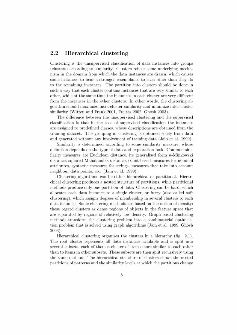
2.2 Hierarchical clustering

Clustering is the unsupervised classification of data instances into groups(clusters) according to similarity. Clusters reflect some underlying mecha-nism in the domain from which the data instances are drawn, which causessome instances to bear a stronger resemblance to each other than they doto the remaining instances. The partition into clusters should be done insuch a way that each cluster contains instances that are very similar to eachother, while at the same time the instances in each cluster are very differentfrom the instances in the other clusters. In other words, the clustering al-gorithm should maximize intra-cluster similarity and minimize inter-clustersimilarity (Witten and Frank 2001, Freitas 2002, Ghosh 2003).

The difference between the unsupervised clustering and the supervisedclassification is that in the case of supervised classification the instancesare assigned to predefined classes, whose descriptions are obtained from thetraining dataset. The grouping in clustering is obtained solely from dataand generated without any involvement of training data (Jain et al. 1999).

Similarity is determined according to some similarity measure, whosedefinition depends on the type of data and exploration task. Common sim-ilarity measures are Euclidean distance, its generalised form n-Minkowskidistance, squared Mahalanobis distance, count-based measures for nominalattributes, syntactic measures for strings, measures that take into accountneighbour data points, etc. (Jain et al. 1999).

Clustering algorithms can be either hierarchical or partitional. Hierar-chical clustering produces a nested structure of partitions, while partitionalmethods produce only one partition of data. Clustering can be hard, whichallocates each data instance to a single cluster, or fuzzy (also called softclustering), which assigns degrees of membership in several clusters to eachdata instance. Some clustering methods are based on the notion of density:these regard clusters as dense regions of objects in the feature space thatare separated by regions of relatively low density. Graph-based clusteringmethods transform the clustering problem into a combinatorial optimisa-tion problem that is solved using graph algorithms (Jain et al. 1999, Ghosh2003).

Hierarchical clustering organises the clusters in a hierarchy (fig. 2.1).The root cluster represents all data instances available and is split intoseveral subsets, each of them a cluster of items more similar to each otherthan to items in other subsets. These subsets are then split recursively usingthe same method. The hierarchical structure of clusters shows the nestedpartitions of patterns and the similarity levels at which the partitions change

8

(Jain et al. 1999, Freitas 2002).

Figure 2.1: Data structure produced by hierarchical clustering. Elements inthe clusters on a lower level are more similar to each other than elements in

the clusters on a higher level.

Hierarchical clustering algorithms can be either agglomerative or divi-sive. Agglomerative algorithms begin with each data instance as the smallestpossible clusters and then successively merge the clusters together until astopping criterion is satisfied. Divisive algorithms begin with the completedataset as one large cluster and perform splitting until some stopping crite-rion is reached. Most hierarchical clustering algorithms are variants of thesingle-link, complete-link or average-link algorithms. These differ in the waythe similarity between two clusters is defined. In the single-link method thedistance between two clusters is the minimum of the distances between allpairs of data instances from the respective clusters. In the complete-linkalgorithm the distance between two clusters is the maximum of all pair-wisedistances between data instances in both clusters. The average-link algo-rithm takes the average pair-wise distance between objects in two clustersas the inter-cluster similarity (Jain et al. 1999, Ghosh 2003).

2.3 Self-Organising Map (SOM)

Artificial neural networks (ANNs) are quantitative methods for data explo-ration and are based on the simulation of the functions of biological nervoussystems. Biological systems consisting of large ensembles of neurons per-form extraordinarily complex computations by having the ability to learn atask over time. This property makes them attractive as a model for com-putational methods designed to process and analyse complex data (Silipo2003).

ANNs represent a family of models rather than a single method. Thesimplest and historically first developed neural network is the perceptron,

9

which is a feed-forward neural network with one layer of neurons. Networkswith more than one layer of artifical neurons, where only forward connectionsfrom the input towards the output are allowed, are called Multilayer Per-ceptrons or Multilayer Feedforward Neural Networks. With their trainingprocedure in the form of backpropagation algorithm they have been success-fully used for solving difficult and diverse problems including a wide range ofclassification, prediction and function approximation problems. Other typesof neural networks have been developed for other types of problems, such asanalysis of time series data or reduction of data dimensionality. An exam-ple of a network that reduces dimensionality by implementing a non-linearprojection of the multidimensional input data onto a two-dimensional arrayof neurons is a Self-Organising Map (Silipo 2003, Si et al. 2003)

A Self-Organising Map (SOM) maps multidimensional data onto a low-dimensional space while preserving the probability density and the topologyof the input data. It is an unsupervised learning network and producesclustering of multidimensional input data. This means that the training dataitems do not have any categorical information provided and are assignedto spatial clusters only on the base of their similarity. Unlike supervisedmethods which associate a set of inputs with a set of outputs using a trainingdataset for which both input and output are known, the SOM uses similarityrelationships in the data to separate the input data vectors into clusters(Kohonen 1997, Si et al. 2003).

Figure 2.2: The neighbourhood function hck(t) of a SOM, centred over thebest matched neuron mc.

The SOM algorithm defines a mapping from the input data space Rn

onto a two-dimensional array of nodes, represented as a lattice of neurons.

10

Figure 2.3: The Self-Organising Map. Input data vector x is connected to allneurons in the lattice. The best matched neuron mc for this particular datavector is shown as a black circle and the neighbour neurons that are affected

by this best match are shown in grey. Other neurons are not affected.

The lattice type of the array can be rectangular, hexagonal or irregular.With every node i a reference vector of weights mi = [µi1, µi2, . . . , µin] ∈ R

n

is associated. When a data object x ∈ Rn is inserted into the system, it

is compared with the reference vectors mi of all neurons. The response ofthe system is the location of the neuron that is most similar or the bestmatch to the input data vector x in some metrics. This response definesa non-linear projection of the probability density function p(x) of the n-dimensional input data vector x onto the two-dimensional display. Theprojection is formed during the learning stage (training), when after eachinput the weight vectors mk of each neuron in a neighbourhood of the outputneuron mc (best match) are recalculated as:

mk(t + 1) := mk(t) + hck(t) · ‖x(t) − mk(t)‖.Here ‖x(t) − mk(t)‖ is the difference between the input vector x and theneuron mk. The expression hck(t) is a neighbourhood function, which iscentred on the best matched neuron mc for the input data vector x. Theneighbourhood function is a smoothing kernel defined over the lattice pointsthat reaches the highest value at the best matched neuron mc and monotoni-cally decreases towards 0 with distance from the central neuron. An exampleof a neighbourhood function is shown in fig. 2.2. In other words, cells thatare topographically close in the array up to a certain geometric distance willactivate each other to learn something from the same input data vector x(fig. 2.3). The spatial ordering of the output map is therefore such that

11

similar input patterns are mapped to neurons that are close to each otherin the output map. This is the topology preserving property. SOM also hasa distribution preserving property, to allocate the data items that appearmore frequently during the training phase to nearby cells (Kohonen 1997).

12

Chapter 3

The role of visualisation in data mining

Most contemporary databases contain large amounts of multidimensionaldata, which makes finding the valuable information a difficult task. Withtoday’s automatic data mining systems it is only possible to examine rel-atively small portions of data. Having no possibility to explore the largeamounts of collected data makes them useless and the databases becomedata dumps. This is where visual data analysis can become useful (Keimand Ward 2003).

Another issue regarding automatic data mining is that the user has beenestranged from the process of the data exploration. The process has becomemore difficult to comprehend for the user, who has to understand boththe structure of the data and the complex mathematical background of theexploration process (Keim 2001).

Visualisation can contribute to the data mining process in two ways.First, it can provide visual display of the results of complicated computa-tional algorithms. Second, it can be used to discover complex patterns indata which are not detectable by current computational methods, but whichcan be identified by the human visual system. The first approach is to vi-sualise results of automatic data mining algorithms. The second approachis visual data mining. This chapter gives an introduction to data visualisa-tion and then discusses both approaches to combine visualisation and datamining.

3.1 Data visualisation

When exploring data, humans look for structures, patterns and relationshipsbetween data elements. Such analysis is easier if the data are presented ingraphical form - in a visualisation. Information visualisation is defined asthe use of interactive visual representation of abstract data to amplify cog-nition (Shneiderman and Plaisant 2005). It is the graphical (as opposed totextual or verbal) communication of information, data, documents or struc-ture. It fulfils various purposes: it provides an overview of complex and largedatasets, shows a summary of data and helps in the identification of possi-ble patterns and structures in the data. The goal of the visualisation is toreduce the complexity of a given dataset, while at the same time minimizing

13

the loss of information (Fayyad and Grinstein 2002).Interaction is a fundamental component of visualisation that permits the

user to modify the visualisation parameters. The user can interact with thedata in a number of different ways, such as browsing, sampling, querying,manipulating the graphical parameters, specifying data sources to be dis-played, creating the output for further analysis or displaying other availableinformation about the data (Grinstein and Ward, 2002).

Visualisation methods can be either geometric or symbolic. The data arein a geometric visualisation represented using lines, surfaces or volumes. Insuch case the data are most often numeric and were obtained from a physicalmodel, simulation or computation. Symbolic visualisation represents non-numeric data using pixels, icons, arrays or graphs (Grinstein and Ward2002).

A more general classification of visualisation methods is presented byKeim (2001) and by Keim and Ward (2003). They construct a three-dimensional visualisation space by classifiying the data according to threeorthogonal criteria: the data type, the type of the visualisation method andthe interaction method (fig. 3.1). Keim defines the following data types:one-dimensional data, two-dimensional data, multidimensional data, textand hypertext, hierarchies and graphs and finally algorithms and software.The interaction methods are projection, filtering, zooming, distortion andbrushing and linking. The visualisation types are standard 2D/3D displays,geometrically transformed displays, icon-based displays, dense pixel displaysand hierarchical displays. In the following we briefly describe each visuali-sation type and list some examples.

Standard 2D/3D displays are well known and commonly used. Theyinclude the mathematical representations of one to four-dimensional data ina two or three-dimensional orthogonal coordinate system. Some examplesof this type of visualisations are line graphs and isosurfaces, a histogram, akernel plot, a box-and-whiskers plot, a scatterplot, a contour plot, and a piechart (Hand et al. 2001, Grinstein and Ward 2002).

The aim of geometrically transformed visualisations is to find an interest-ing geometric projection of a multidimensional dataset onto the two displaydimensions. Due to the many possibilities of mapping multidimensionaldata on the two-dimensional screen, this group includes a large variation ofvisualisation methods (Keim 2002).

A typical example of a geometrically transformed visualisation is a scat-terplot matrix, which is a generalisation of the scatterplot into n dimen-sions. Scatterplots for each pair of dimensions are created and arrangedinto a matrix. Points corresponding to the same object are highlighted in

14

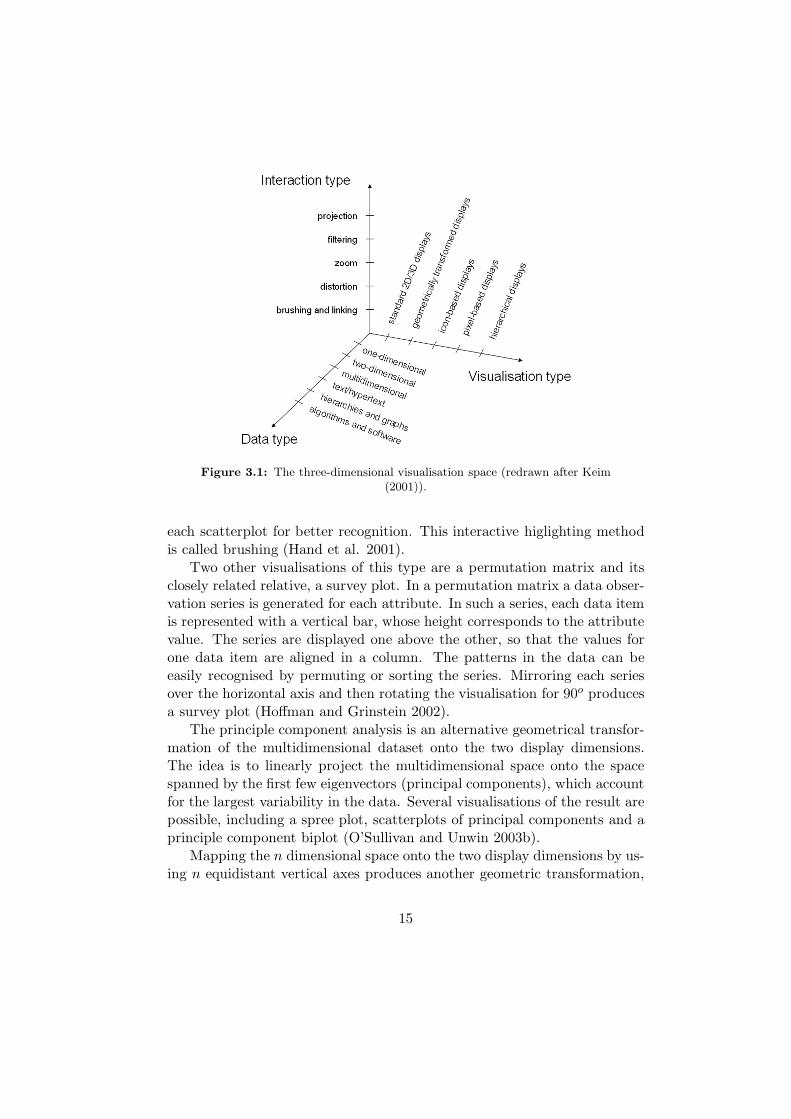
Figure 3.1: The three-dimensional visualisation space (redrawn after Keim(2001)).

each scatterplot for better recognition. This interactive higlighting methodis called brushing (Hand et al. 2001).

Two other visualisations of this type are a permutation matrix and itsclosely related relative, a survey plot. In a permutation matrix a data obser-vation series is generated for each attribute. In such a series, each data itemis represented with a vertical bar, whose height corresponds to the attributevalue. The series are displayed one above the other, so that the values forone data item are aligned in a column. The patterns in the data can beeasily recognised by permuting or sorting the series. Mirroring each seriesover the horizontal axis and then rotating the visualisation for 90o producesa survey plot (Hoffman and Grinstein 2002).

The principle component analysis is an alternative geometrical transfor-mation of the multidimensional dataset onto the two display dimensions.The idea is to linearly project the multidimensional space onto the spacespanned by the first few eigenvectors (principal components), which accountfor the largest variability in the data. Several visualisations of the result arepossible, including a spree plot, scatterplots of principal components and aprinciple component biplot (O’Sullivan and Unwin 2003b).

Mapping the n dimensional space onto the two display dimensions by us-ing n equidistant vertical axes produces another geometric transformation,

15

a parallel coordinates plot. The axes correspond to the dimensions and arelinearly scaled from the minimum to the maximum value of the correspond-ing dimension. Each data item is then drawn as a polygonal line intersectingeach of the axes at the point which corresponds to the data value (Inselberg2002).

Icon-based display methods visualise multidimensional data by mappingthe attribute values of each data element onto features of an icon (Hoffmanand Grinstein 2002).

One of the most commonly used icon-based visualisations are star icons.In a star icon lines in different directions emanating from a central pointrepresent different dimensions, while the length of the radius in each direc-tion represents the value in the respective dimension. The icons are usuallyarranged on the display in a grid manner (Grinstein and Ward 2002).

Another well-known iconic visualisation are Chernoff faces. Human be-ings have a highly developed ability to perceive subtle changes in facialexpressions. Even in a very simplified drawing of a face a small differenceis registered as a difference in emotion. This ability has been applied topattern recognition for multidimensional data. The dimensions are mappedto the properties of a face icon - the shape of the eyes, nose and mouth andthe shape of the face itself (Ankerst 2000).

Other examples of icon-based visualisations include stick figure icons,colour icons and tile bars (Hoffman and Grinstein 2002).

Dense pixel visualisations map each data item to a coloured pixel andgroup the pixels belonging to each dimension into adjacent areas. Thesevisualisations allow displays of the largest amount of data among all visual-isations, because they use up only one pixel per data item (Keim 2002).

One example of a dense pixel display is a recursive pattern visualisa-tion, which is based on a recursive forth and back arrangement of the pixelsand is aimed at representing data with a natural order according to oneattribute, such as for example time series. Attributes are presented as rect-angles in a grid, where in each rectangle the pixels are ordered according toone attribute along a snake-like curve. The visualisation is called a circlesegment view if the attributes are presented as circle segments instead ofthe rectangles (Keim et al. 2002).

Another idea is to colour pixels inside graphic entities of a univaritevisualisation according to some other attribute. An example of this principleis a space-filling Pixel Bar Chart visualisation. If more than one additionalattribute is to be presented, the ordering of pixels can be represented byone attribute. Several bar charts are then produced in which the colouringis defined according to some third attribute. This visualisation is called

16

Multi-pixel Bar Charts (Keim et al. 2003a).Hierarchical visualisations are used to represent a hierarchical partition-

ing of the data (Keim 2002). Examples include dendrograms, structure-based brushes, Magic Eye View, treemaps, sunburst and H-BLOB. Theseare described in the next section, where we discuss visualising results of au-tomatic data mining algorithms - in particular visualising the structure thatis the result of hierarchical clustering.

3.2 Visualising results of automatic data mining

algorithms

Once the data mining algorithm has been applied to the dataset, the amountof patterns generated usually exceeds the number that can be interpretedand evaluated in textual form. Communicating the results of the mining iscrucial, regardless if the project calls for a predictive, classificatory, explana-tory, exploratory, scenario planning, strategic, tactical or any other type ofmining task. In the end the discovered complex relationships have to beexplained and this is usually done in visual form. Visualisation serves as apost-processing communication channel between the user and the computerthat brings the discovered information to the user (Ankerst 2000, Pyle 2003).

There are numerous visualisation methods developed to display results ofthe different automatic data mining algorithms. In the following we presentan overview of methods that are relevant for this thesis, for visualising resultsof the two data mining algorithms that were used in case studies: hierarchicalclustering and SOM.

3.2.1 Hierarchical clustering

Hierarchy of the data obtained from hierarchical clustering can be repre-sented explicitly or implicitly. Explicit methods represent the edges betweenthe elements of the hierarchy. This group includes all variations of dendro-grams. Implicit methods show relations between elements by special spatialarrangements of elements. Space-filling methods and methods using implicitsurfaces belong in this group (Keim et al. 2002).

The simplest way in which a hierarchical structure can be representedis a dendrogram. A dendrogram is a mathematical tree. The root vertex ofsuch a tree represents all data instances. The dataset is split into severalsubsets, each of them a cluster of items more similar to each other than toitems in other subsets. These clusters form the child vertices of the root.

17

The child vertices are split recursively using the same similarity criterion.The data items are represented as leaves on the lowest levels in the treestructure, whereas the vertices higher up in the tree represent clusters ofdata items at different levels of similarity (Muller-Hannemann 2001).

The classical way to visualise a dendrogram is to draw it as a top-down rooted-tree, with the root anchored centrally on the top of the displayand the children vertices drawn downwards using straight or bended lines(Muller-Hannemann 2001), such as for example in fig. 3.2. This classicaldisplay can become unclear and messy at the leaf level when a lot of dataitems are present. To solve this a dendrogram can be connected with othervisualisations, for example, with a scatterplot (Seo and Shneiderman 2002).It can also be mapped on some surface other than a usual 2D plane in orderto produce a clearer visualisation. When draped on a hemisphere it is calledThe Magic Eye View. The projection of the hemisphere from a different an-gle to the 2D equatorial plane can be used to produce a zoomed focus view,enlarging a part of the structure that is closer to the angle of projection(Kreuseler and Schumann 2002).

Figure 3.2: A dendrogram.

Implicit methods for visualising the hierarchical structure in the data are,for example, a treemap and a sunburst. A treemap divides the display areainto a nested sequence of rectangles representing vertices of the dendrogram.The root vertex is represented by the outer rectangle. At each recursive stepthe rectangle representing the current vertex is sliced by parallel lines intosmaller rectangles representing its children. At each level of the recursion the

18

orientation of the lines is switched from horizontal to vertical or vice versa(Bederson et al. 2002). A sunburst visualisation shows the hierarchicalstructure of the data in a radial layout. A small circle in the centre of thevisualisation represents the root of the hierarchy. For each recursive level aring is added to the display. The rings are subdivided in sectors accordingto the number and size of the children on the respective level. The childrenare drawn within the arc belonging to their parent vertex (Stasko and Zhang2000).

Another implict way to represent a hierarchical structure is by nestedthree-dimensional isosurfaces. An example of such a visualisation is H-BLOB. The clusters are visualised by a hierarchy of implicit isosurfaces,which are wrapped around the groups of points belonging to the same clus-ter (Sprenger et al. 2000).

3.2.2 Visualising the result of a SOM

The methods for visualising the result of a SOM can be divided into severalcategories according to the display goal.

The SOM visualisations in the first category provide the possibility toidentify the shape and the cluster structure of the dataset. This groupincludes visualistions based on projections and distance matrices (Vesanto1999).

Projection visualisations show data items projected as points in two orthree dimensions. The points are linked to a SOM lattice through a colourscheme of neurons in the lattice. The colour is transferred to the data objectsin the projection, thus indicating which objects belong to which cluster indifferent areas of the lattice (Vesanto 1999).

Most SOM visualisations are based on distance matrices. The mostwidely used distance matrix is the U-matrix, where SOM cells are repre-sented as either rectangular or hexagonal cells in a two-dimensional lattice.The distances of each cell to each of its immediate neighbours are calculatedand used to assign a grey level to each of the cells. Light areas in such amap indicate that the cells in this area are similar to each other and repre-sent a cluster. Neighbouring neurons in dark areas are not that similar toeach other, which marks borders between clusters. Clusters can be indicatedusing other visual variables as well, for example the size of the cells or theappearance of the border lines between the cells. If the intention is to showthe similarity of the cells rather than the cluster structure, the colour huecan be used. A colour is assigned to each cell so that similar map unitsreceive similar colours (Kohonen 1997, Vesanto 1999).

19

The second group of SOM visualisations was designed for analysing thecharacteristics of clusters and correlations between data attributes. Onesuch visualisation are the component planes. Each component plane is theneural lattice, where one graphic variable of the cells represents the valuesof a particular attribute. Attribute values are usually represented by thegrey level or colour of the cell. All planes are arranged in the display sothat they can be compared to each other. Correlations between attributesare revealed as similar patterns at identical positions in different componentplanes (Vesanto 1999). Koua and Kraak (2004b) present an application ofthe component planes SOM visualiation.

Another possibility to display the result of a SOM for correlation anal-ysis is to show the distance between neurons as the heights of a three-dimensional surface. The original lattice with grey shades/colours or any ofthe component planes can be draped over such a surface. Applications ofthis visualisation are presented in Takatsuka (2001) and Koua and Kraak(2004b).

An alternative three-dimensional approach is to use a 3D spherical Self-Organising Map, where the lattice of the usual two-dimensional SOM isreplaced by a unit sphere, tesselated into three-dimensional uniform tri-angular elements. Once the 3D SOM is trained, the resulting structure ismapped to the shape of the elements, which are distorted in order to visuallyrepresent associations in the data. Distortions in the triangular 3D latticeare created by scaling the radial distance of the nodes in proportion to thesimilarity measure. The surface enclosing the 3D lattice is then coloured bymapping the magnitude of the measure to lie within the visible range of theelectromagnetic spectrum. The final visualisation is a 3D distorted sphere,where elevation goes from blue in the valleys to red in the peaks, indicatingthe clusters in the data (Sangole and Knopf 2003).

3.3 Visualisations relevant to this thesis

This section describes the visualisations that are the building blocks forthe exploratory systems in the three case studies in this thesis. They arelisted in table 3.1. Visualisations in all three case studies were interactivelyconnected by the principle of brushing and linking. This means that when asubset of data elements was highlighted or selected in one visualisation, thesame elements were highlighted or selected everywhere, providing a bettervisual impression and easier pattern recognition.

20

Table 3.1: Visualisations used in the three case studies in this thesis: H -histogram, P - pie chart, SC - scatterplot, SF - spaceFill, GM - geoMap, PCP -parallel coordinates plot, TSPCP - time series parallel coordinates plot, SG -

snowflake graph, SOM - SOM visualisation.

Case Study H P SC SF GM PCP TSPCP SG SOM

1 X X X X2 X X X X X X3 X X X X X X

A histogram is the most common method for visualisation of data ob-jects with a single dimension. It maps the number of data instances witha particular attribute value to the height of a rectangular bar assigned tothe respective attribute value or a range of values. Histogram belongs tothe group of standard 2D/3D display methods. It provides a descriptionof the distribution of the data and helps with identification of suspiciousdata records and outliers. These can consequently be removed from furtheranalysis. The reliability of the method increases with the number of pointsin the sample, giving a more realistic picture on big data sets. The methodis less reliable for small data sets, because it shows unrealistic random fluc-tuations if the data sample is not carefully chosen (Hand et al. 2001). Anexample of a histogram for uranium concentration is shown in fig. 3.3 andwas produced with data from Paper IV.

Figure 3.3: A histogram of uranium concentration.

A pie chart is a visualisation of one attribute and belongs in the groupof the standard 2D/3D display methods. It shows the proportional size ofvalues of the chosen attribute, represented by angular segments of a circle.The segments are usually displayed in different colours. A typical pie chartwith a legend is illustrated in fig. 3.4 and was produced for a metadata

21

attribute THEME in case study 1. The visualisation is useful for recognisinga dominant value of the attribute (StatSoft 2006).

Figure 3.4: A piechart, indicating ”planning” as the dominant value in theattribute THEME.

A scatterplot is a visualisation of two-dimensional data. Each dimensionis assigned to one of the two axes and all data items are then plotted intothe display area as points located at appropriate positions according to theirrespective attribute values. The visualisation is appropriate for discoveringcorrelation between the two portrayed attributes, but it has the disadvantageof showing unrealistic patterns, when there are too many data points andoverprinting occurs. Overprinting conceals the strength of actual correlationbetween the attributes (Hand et al. 2001). The scatterplot is a standard2D/3D display. An example of a scatterplot of elevation in slope for datafrom Paper IV is shown in fig. 3.5. The colour of the data points in thispicture is assigned according to some third attribute and in this case servesto visually indicate the high level of oveprinting.

Another bivariate visualisation used in case studies 2 and 3 is a spaceFillvisualisation, which is related to pixel-based display methods. The spaceFilldisplays data in a grid, where each grid square represents one data element.The visualisation solves the problem of overprinting, as it displays all dataelements at non-overlapping positions (MacEachren et al. 2003). A space-Fill can be used to visually estimate the strength of the relationship betweenthe two displayed attributes. The colour in the spaceFill is assigned accord-ing to one attribute. The second attribute defines the order of the grid cells:the cell with the lowest value for this attribute is situated in the bottom-leftcorner, from where the cells proceed along a scan line towards the cell withthe highest attribute value in the top-right corner. If the attribute definingthe colour of the cells is strongly correlated with the attribute defining theorder of the cell, there is a relatively regular and smooth transition from the

22

Figure 3.5: A scatterplot of elevation and slope.

lightest to the darkest colour from bottom to top (or from top to bottom). Aweaker correlation produces a scattered pattern. A random pattern meansthat there is no correlation between the respective attributes. This is justa visual estimation, but the observation can be used to form a hypothesis,which could then be explored further using other tools, for example statis-tics or spatial analysis (Paper V). An example of a spaceFill visualisationproduced in case study no. 3 is shown in fig. 3.6.

Figure 3.6: A spaceFill visualisation showing density of night-time accidentsvs. density of bars and restaurants.

The spatial visualisation in case studies 2 and 3 was a geoMap. This isa bivariate choropleth map, whose colour scheme depends on two attributes(Gahegan et al. 2002, Takatsuka and Gahegan 2002). Fig. 3.7 shows an

23

example of the geoMap for the emergency response data in case study 3.

Figure 3.7: A bivariate geoMap showing population density vs. density ofnight-time incidents.

Bivariate visualisations used in case studies 2 and 3 were grouped into amultiform bivariate matrix, which is a generalisation of a scatterplot matrix.An element in the row i and column j in a multiform bivariate matrix isa scatterplot of the variables i and j, if it is located above the diagonal, aspaceFill visualisation of the same two variables, if it is located below thediagonal and a histogram of variable i, if it is on the diagonal (MacEachrenet al. 2003). An example of the multiform bivariate matrix showing 11attributes of the data from case study 2 is shown in fig. 3.8.

A parallel coordinates plot (PCP), used in all three case studies, is a ge-ometrically transformed visualisation, which maps the m-dimensional spaceonto the two display dimensions by using m equidistant vertical axes. Theaxes correspond to the dimensions and are usually linearly scaled from theminimum to the maximum value of the corresponding dimension. Each dataitem is presented as a polygonal line intersecting each of the axes at the pointwhich corresponds to the data value. The PCP reveals a wide range of datacharacteristics, such as different data distributions, clusters in the data andfunctional dependencies. There is one disadvantage: overprinting of polygo-nal lines can occur when displaying large amounts of data (Inselberg 2002).An example of a PCP is shown in fig. 3.9. It shows a PCP of seven at-tributes (i.e. m = 7) from case study 2, where colour has been assigned tothe polygonal lines according to the last attribute.

A parallel coordinates plot can also be used as a temporal visualisation.

24

Figure 3.8: A multiform bivariate matrix with 11 attributes.

In this case, each axis is assigned to a specific variable at a specific time.This variation, the time series parallel coordinates plot (TSPCP) is usefulfor visualising temporal trends (Edsall 2003a) and was used in case study 3to show the temporal component of the incidents data (Paper V).

Figure 3.9: A parallel coordinates plot of seven attributes.

In case study 1 a special hierarchical visualisation, called a snowflakegraph, was developed and implemented. The snowflake graph is a versionof a dendrogram, which is drawn as a radial tree, so that the root of thetree is placed in the centre of the image. This is in contrast with traditionaltop-down tree-drawing methods, which anchor the root of the tree in thecentre of the upper edge. The structure is recursively drawn (fig. 3.10):

25

each vertex is the centre of a circle, its incoming edge and outgoing edgesare evenly distributed in this circle, and the child vertices are placed on thecircumference of the circle (Paper III).

Figure 3.10: The recursive construction of the snowflake graph (Paper III).

The similarity of the data elements is represented in two ways in thesnowflake graph. In the hierarchical tree the data elements whose leaf-to-root paths meet in a near-by ancestral vertex are more similar to each otherthan those data elements, whose leaf-to-root paths meet higher up in thetree. A colour scheme for the edges and vertices was added to this naturalstructure. The colour was defined in two steps (fig. 3.11). The child verticesof the root and their respective incoming edges are coloured according totheir position in the hue circle. The colour for all other vertices is derivedfrom the colour of their parent vertex in the following way: the hue ofthe child’s colour remains the same as the hue of the parent, whereas thesaturation and brightness of children change linearly. In this way verticesthat belong to similar data elements or clusters receive similar colours (PaperIII).

The SOM visusalisation used in case study 2 was based on a distancematrix. It is shown in fig. 3.12. Here the distance matrix is represented asa hexagonal lattice. Changes in three visual variables indicate the clusterstructure, the similarity of data objects and the distribution of the dataobjects in the SOM cells. The cluster structure is shown by the grey level of

26

Figure 3.11: Assigning colour to the root vertex and all other vertices in thesnowflake graph (Paper III).

Figure 3.12: SOM visualisation as a hexagonal U-matrix.

the cells. Circles of various colours are projected in a regular pattern overthe grey hexagonal cells in order to indicate the similarity and distributionof the data objects. The colour of the circles indicates similarity: cells thatare more similar to each other receive a more similar colour. The datadistribution in the cells is indicated by the size of the circles: the larger thecircle the more data objects have been mapped to the cell that the circlebelogns to. The visualisation has been produced with the data exploration

27

system from Paper IV and comes from GeoVISTA Studio (Gahegan et al.2002, Takatsuka and Gahegan 2002).

3.4 Visual data mining

All data mining is a form of pattern recognition. The most formidable pat-tern recognition apparatus is the human brain. It is so powerful that itwill recognise patterns even where none exist. Human ability of perceptionenables the analyst to analyse complex events in a short time interval, recog-nise important patterns and make decisions much more effectively than anycomputer can do. The question is how to enable this formidable appara-tus to work in data mining process. Given that vision is a predominantsense and that computers have been created to communicate visually withhumans, computerised data visualisation provides an efficient connectionbetween data and mind (Ankerst 2000, Pyle 2003, Keim and Ward 2003).

The integration of visualisation in the data mining process is often re-ferred to as visual data mining. The basic idea of visual data mining is topresent the data in some visual form, in order to allow the human to getinsight into the data, draw conclusions and directly interact with the data.The process of visual data mining can be seen as a hypothesis generatingprocess: after first gaining the insight into data, the user generates a hy-pothesis about the relationships and patterns in the data (Ankerst 2000,Keim 2002).

Visual data mining can be used for either confirmative or explorativedata analysis. In confirmative analysis the user already has some idea whathe is looking for and only needs to confirm a prior hypothesis. Explorativeanalysis starts with data about which the user has no knowledge. By usinginteractive exploration, which is usually an undirected search for structuresor trends in an appropriate visualisation, the user forms hypotheses, whichcan then be confirmed by other data analysis methods (Ankerst 2000).

Visual data mining has several advantages over the automatic data min-ing methods. It leads to a faster result with a higher degree of human confi-dence in the findings, because it is intuitive and requires less understandingof complex mathematical and computational background than automaticdata mining. It is effective when little is known about the data and the ex-ploration goals are vague, since these can be adjusted during the explorationprocess. Using the visual approach it is possible to explore heterogeneousand noisy data. Visual mining can provide a qualitative overview of the dataand allow unexpectedly detected phenomena to be pointed out and explored

28

using further quantitative analysis (Keim et al. 2004)The visual data mining process starts by forming the criteria about which

visualisations to choose and which attributes to display. These criteria areformulated according to the exploration task. The user recognises patternsin open visualisations and selects a subset of items that he/she is interestedin. The selection is performed simultaneously in all open visualisations.The result of this selection is a restriction of the search space which mayshow new patterns to the user, some of which he/she might not have beenaware of before. The whole process can then be repeated on the selectedsubset of data items. Alternatively, new visualisations can be added. Theprocess continues until the user is satisfied with the result, which representsa solution to his/her initial problem. The interaction between the user andthe computer and the simultaneous selection of data in all visualisationsform a dynamic process that can be iteratively repeated until a satisfactoryoutcome has been found. The user has full control over the exploration byinteracting with the visualisations (Paper I). The process is illustrated infig. 3.13.

Figure 3.13: The visual data mining process.

Visual data mining has been used in a number of scientific disciplines.Some recent examples include detecting telephone call frauds by a combina-tion of directed graph drawings and barplots (Cox et al. 1997), a classifierbased on a parallel coordinates plot (Inselberg 2002) and a visual mining ap-proach by applying 3D parallel histograms to temporal medical data (Chit-taro et al. 2003).

3.5 Combining automatic and visual data mining

Automatic data mining is primarily centred on number crunching methodswith minimal user involvement, as the computer attempts to extract vari-ous features of the data. Visual data mining has emphasis on user interac-

29

tions and manipulations of graphical data representations for visual featurerecognition and understanding. Each approach has its advantages and weak-nesses. Whereas automatic algorithms working in isolation can easily missout on the wisdom that is readily available from human knowledge of theexploration problem and the data, manually guided visual approaches easilycause users to lose their way in high dimensional spaces. Efficient extrac-tion of hidden information requires skilled application of complex algorithmsand visualisation tools, which must be applied in an intelligent and thought-ful manner based on intermediate results and background knowledge. Thewhole knowlege discovery process is therefore difficult to automate, as itrequires a high-level intelligence at its centre. By merging automatic andvisual mining the flexibility, creativity and knowledge of a person are com-bined with the storage capacity and computational power of the computer.A combination of both automatic and visual mining in one system per-mits a faster and more effective knowledge discovery (Miller and Han 2001,Kopanakis and Theodoulidis 2003).

Combining automatic and visual data mining is usually done by integrat-ing a visualisation of the result of an automatic mining method in the visualdata mining system. A review of integrated visualisation and algorithm sys-tems for association rules, classification and clustering is presented in Keimet al. (2002). Some other selected applications include a combination of hi-erarchy computation and Self-Organising Map with hierarchy visualisationon a sphere called the Magic Eye View (Kreuseler and Schumman 2002)and a combination of a visual clustering method based on the single valuedecomposition and a validation methodology used for assessing the clusterstructure (Manco et al. 2004). Kimani et al. (2004) present a visual datamining environment with visualisations for clustering and association rules.Association rules are visualised in several systems by either bar charts, gridsand a parallel coordinates plot (Kopanakis and Theodoulidis 2003), by 3Dgraphical representations (Kopanakis et al. 2005) and by graph drawingsand a parallel coordinates plot (Buono and Costabile 2005).

Visual data mining alone and in combination with automatic methodshas also been used for geospatial data. A review of geographic applicationsis presented in the next chapter.

30

Chapter 4

Data mining for geospatial data

4.1 Spatial data mining

Spatial analytical methods traditionally used for exploring geospatial datawere developed at a time when datasets were small. They are confirmatory,require a priori hypotheses and are focused on obtaining scarce informationfrom the small datasets. They are not meant to discover new unexpectedpatterns, trends and relationships that can be hidden in very large andheterogeneous geospatial datasets. This is where data mining comes intoplay, as an appropriate tool for extracting patterns from large geospatialdatabases (Miller and Han 2001, Shekhar and Chawla 2003).

The requirements for mining geospatial data are different from those formining classical relational databases. The reason for this are the specialproperties of spatial data: high dimensionality, spatial autocorrelation, he-terogeneity, complexity, ill-structured data and dependence on scale (Fothe-ringham et al. 2000, Miller and Han 2001, Shekhar and Chawla 2003).

Spatial information is not only multidimensional, but also has the proper-ty that up to four dimensions of the information space are interrelated andprovide a measurement framework for all other dimensions. Computationalrepresentations of spatial information require an implied topological andgeometric measurement framework which affects the patterns that can beextracted.

Geospatial data are spatially dependent. Spatial dependency is the ten-dency of attributes at some location in space to be related. This property ofgeographic phenomena that similar things cluster in space is so fundamentalthat geographers have elevated it to the status of the first law of geography(Tobler’s law): ”Everything is related to everything else, but nearby thingsare more related than distant things”. This characteristics is called spatialautocorrelation in spatial statistics.

Spatial heterogeneity refers to the non-stationarity of most geographicprocesses, meaning that most geographic processes vary by location andthat it is not possible to describe the phenomenon well at any location usinga global estimate of parameters.

Spatio-temporal objects and relationships tend to be more complex thanthe objects and relationships in non-spatial databases. Size, shape and

31

boundary properties of geographic objects affect relationships such as dis-tance, direction and connectivity.

Spatial data are developing beyond the traditional raster and vectorformats, including ill-structured data, such as imagery and geo-referencedmultimedia.

Finally, there is the issue of scale. The level of aggregation at whichthe spatial data are being analysed is very important for the data miningprocess. Identical spatial analysis experiments at different levels of scale cansometimes lead to contradictory results.

These properties of spatial data make classical data mining algorithmsinappropriate for mining spatial data. Classical data mining techniques as-sume that the data are independently generated and identically distributedover space. This is contradicted by spatial autocorrelation and spatial hete-rogeneity in the case of geospatial data. These two properties have been tra-ditionally regarded as a nuisance for classical data mining methods. Nowa-days they are recognised as a potentially valuable source of informationabout the geographic phenomenon under investigation and should be takeninto account in the process of knowledge discovery (Fotheringham et al.2000, Shekhar and Chawla 2003).

Automatically extracting knowledge from spatial data therefore requiresspecial approaches. There are two main ways to do that. The first one isto invent new spatially aware algorithms that are particularly adapted toexplore spatial data. The second one is to explicitly model spatial proper-ties and relationships in the pre-processing step and then use classical datamining algorithms (Shekhar and Vatsavai 2003).

Examples of spatially aware algorithms are spatial regression, spatial as-sociation rules (SAR), Markov Random Fields (MRF) Bayesian classifier,colocation rules, spatial clustering for large datasets and spatial outlier de-tection methods (Shekhar and Chawla 2003, Shekhar and Vatsavai 2003).Further examples include spatial clustering (Han et al. 2001a), spatial as-sociation rules-based classification SPARC (Han et al. 2001b) and spatialsubgroup discovery algorithm (May and Ragia 2002).

Examples of modelling spatial properties combined with classical datamining include applying data mining algorithms on a spatial model producedby paths in neighbourhood graphs (Ester et al. 2000) and modelling spatialdependencies by a contiguity matrix (Chawla et al. 2001). Estivill-Castroand Lee (2001) propose to model the space by a vertical view approach,similar to a virtual raster overlay, and alternatively by a horizontal viewapproach, which polygonises the space by boundary-based graph theoreticalclustering performed on a proximity graph. An association rules algorithm

32

is then applied to the modeled space. Another example of applying asso-ciation rules to a spatially-modeled space uses rough sets theory to modelthe space (Beaubouef et al. 2004). Santos and Amaral (2004) describe spa-tial dependencies (including direction, distance and topological relations)through inferred rules and then apply the decision tree and Self-OrganisingMap algorithms to the spatial model.

Applications of spatial data mining are numerous. Some typical appli-cations are listed in Miller and Han (2001) and include map interpreta-tion, information extraction from remotely sensed imagery, mapping envi-ronment features, extracting spatio-temporal patterns, and analysing inter-action, flow and movement in geographic space.

4.2 Visual data mining for geospatial data

Visual data mining of geospatial data is a part of the growing discipline ofgeovisualisation. Geovisualisation integrates approaches from exploratoryscientific visualisation, cartography, image analysis, information visualisa-tion, exploratory data analysis and geographic information science to pro-vide theory, methods and tools for visual exploration, analysis, synthesisand presentation of geospatial data (Fotheringham 1999, MacEachren andKraak 2001).

Visual data mining has been used for spatial data in a number of cases.Recent examples include visual data mining in atmospheric science (Macedoet al. 2000), visualisations for spatio-temporal data (Dykes and Mountain2003), pixel-based visual data mining (Keim et al. 2003b, Keim et al. 2004),exploration of spatially distributed genetic datasets (Joost and the Econo-gene Consortium 2005) and exploration of biogeochemical data (Grunfeld2005). These examples are here discussed in greater length.

Macedo et al. (2000) present an approach to visually explore a datasetabout ocean atmosphere, including information about sea surface tempe-rature, sea level pressure, wind speed and wind direction. Wind directionplots, maps, scatterplots, variogram clouds and a grand tour dynamic visu-alisation form an interactive exploration system for the atmospheric data.

Dykes and Mountain (2003) explore spatio-temporal data created bymobile communication devices, which represent people’s movements over along time period. Exploration is done by various visualisations, including aninteractive view created by the Location Trend Extractor, density surfacesof recorded spatio-temporal activity (called spotlights), feature networksand geocentric parallel plots, which combine the spatial and statistical com-

33

ponents of quantitative attribute data in instantly updatable graphics inresponse to the movement of the cursor in the map.

Keim et al. (2003b) and Keim et al. (2004) present pixel-based visu-alisations for geospatial data that can be connected in a visual explorationsystem. The main concept is a PixelMap, which is a solution to the prob-lem of overprinting in a dot map, where points are dense in some areas andsparse in other areas. The idea is to reposition the dots that would otherwiseoverlap to neighbouring positions while preserving the overall pattern. Therepositioning is based on kernel-density clustering of geometric parametersand one designated statistical attribute. The dots are coloured according tothe statistical attribute. Other attributes are displayed on additional maps,with data points at the same positions but with colours assigned accordingto other attributes. Dots can be simultaneously highlighted in all maps,which facilitates the exploration.

Joost and the Econogene Consortium (2005) present a complementaryway of analysing genetic data by using geovisualisation. Among other spatialand cartographical tools, a visual data mining system based on geoVISTAStudio (Gahegan et al. 2002) is presented, consisting of thematic maps, aparallel coordinates plot and other interactive visualistations. The approachis evaluated as useful for developing hypotheses about distribution of bio-logical diversity among and within sheep and goat breeds in Europe. It pro-vides the possibility to take into consideration extra-organism informationsuch as geographic location and physical characteristics of the environment,which are usually neglected in the molecular-based DNA analysis methodsfor monitoring and measuring genetic diversity.

Grunfeld (2005) built an exploration system for biogeochemical data con-sisting of various visualisations: a parallel coordinates plot, scatterplot ma-trices, matrices of quartile values of elements and symbol point maps. Thesystem was built for an extensive dataset of lithogeochemical, till geochemi-cal, biogeochemical and moss monitoring data. The purpose was to identifyand characterise natural anomalies in biogeochemical data, for which thesystem proved to be adequate.

4.3 Combining automatic and visual data miningfor geospatial data

One disadvantage of exploring geospatial data visually is that the spatialcomponent of the data is difficult to visualise effectively. The most commongraphic representation of the spatial component in a visual data mining

34

system is a map. However, since the data are often not uniformly distributedover space, some areas on such a map might be sparsely populated whilein other areas a high degree of overprinting occurs. Overprinting couldalso be caused by the sheer size of the dataset. The fact that up to fourdimensions provide a measurement framework for all the other dimensionsalso implies that the graphical representation of geospatial phenomena offersfewer degrees of freedom than are available for the graphical depiction ofarbitrary non-spatial data (Keim et al. 2005, Theus 2005).

When such difficulties occur, it is impossible to rely solely on human vi-sion while exploring the data. Efficient knowledge discovery from geospatialdata is therefore most likely if the advantages of both visual and computa-tional exploration methods are combined. The goal of this integration is toconstruct visually enabled knowledge discovery systems that could facilitatethe automatic process of pattern and relationship recognition in complexdata and the subsequent interpretation of the discovered patterns and re-lationships. Such systems let the analyst visually explore the data withdirect manipulation of the information visualisation components and ap-ply computational tools when something interesting appears. Alternativelycomputational mining can be used as a first pass and the results can then beexamined visually (Shneiderman 2001, MacEachren and Kraak 2001, Dykeset al. 2005).

Currently there exist two environments that support the developmentof both visual and automatic exploration systems. One is the codeless pro-gramming environment GeoVISTA Studio, which allows construction of so-phisticated geoscientific data analysis and visualisation systems. The secondone is an interactive adaptable system CommonGIS, with thematic maps,visualisations of spatio-temporal data and time series data mining methods.

GeoVISTA Studio is a java-based collection of various geographic andother visualisations as well as computational data mining methods. Its com-ponents are implemented as Java Beans, which are self-contained softwarecomponents that can be easily connected into a customised data explorationsystem by visual programming. Furthermore, using Java Beans technol-ogy makes it possible to integrate external methods and own componentsin the system. Available visualisations include a parallel coordinates plot,various bivariate visualisations (scatterplots, spaceFill visualisations, bivari-ate geographic maps, etc.) that can be either independent or elements indifferent types of multiform matrices, time series visualisations and visualclassifiers. Computational methods include a statistics package and severaltypes of classification methods (k-means, ISODATA, maximum likelihoodand a SOM) with respective visualisations. All visualisations and computa-

35

tional components can be interactively connected to each other (Takatsuka2001, Gahegan et al. 2002, Takatsuka and Gahegan 2002, Edsall 2003a,MacEachren et al. 2003).

The CommonGIS system consists of various methods for cartographic vi-sualisation, non-spatial graphs, tools for querying, search and classificationas well as computation-enhanced visual techniques for exploration of spatio-temporal data. Main features are interactive thematic mapping techniques,statistical computations and displays, animated maps, dynamic queries, ta-ble lenses, parallel coordinate plots and time-aware geovisualisation tech-niques. All the tools have a high level of interaction and are dynamicallylinked via highlighting, selection and brushing. The system has been gradu-ally developed over a number of years and used by the authors for geospatialexploration problems originating in such various disciplines as social geogra-phy, forestry, meteorology, seismology, crime and environment (Andrienko Get al. 2003a, Andrienko G et al. 2003b, Andrienko N et al. 2003, AndrienkoG et al. 2004, Andrienko N and Andrienko G 2006).

4.4 Combining spatial and visual data mining

While automatic and visual data mining have been combined and used ongeospatial data in a number of cases, many of these approaches do nottake into consideration geographic knowledge in effective ways, if at all.This is a challenge that demands not just new spatially aware methodsand tools, but requires a fundamental effort in theory building directed tothe representation and management of geographic knowledge (Dykes et al.2005).

Based on the literature survey of spatial and visual data mining there areat the moment only a very few attempts to combine real spatial mining withvisual exploration. One example that could fit into this category is combin-ing a Self-Organizing Map with other visualisations in an explorative system.While a SOM strictly speaking is not a real spatial data mining algorithm,it does preserve both the topology and the distribution of data items in theinput space and is therefore spatially aware to some extent. Using the SOM,similar data are mapped onto the same neuron cell or to neighbour cells inthe two-dimensional output map, which makes it useful as a knowledge dis-covery tool for geographic datasets. One example of this combination is anapproach for exploration of health and demographic data (Koua and Kraak2004a, Koua and Kraak 2004b, Koua 2005). 2D and 3D visualisations of aSOM were also combined with other visualisations in various experiments,

36

from exploring census data to attempting to discover relationships betweenforest structure and landscape (Takatsuka 2001, Gahegan et al. 2002). TheSOM for these components was implemented as a GeoVISTA element. Itsdevelopment, integration into the GeoVISTA environment and an exampleapplication on multidimensional geospatial data is presented by Guo et al.(2005).

Other attempts of integrating spatially aware data mining algorithmswith visual data mining have not been found during the literature survey.Combining spatial and visual data mining is therefore clearly a researchchallenge for the future.

4.5 What this thesis is all about

This thesis investigates how a combination of visual and automatic datamining can be used for exploration of geospatial data in the hypothesisforming process. Three case studies illustrate three different combinationsof methods. Hierarchical clustering is combined with visual data miningfor exploration of geographical metadata in the first case study, which isbased on papers I, II and III. The second and third case studies describeattempts to combine spatial and visual mining. A SOM has been combinedwith several multivariate visualisations for exploring environmental data incase study 2, presented in paper IV. Case study 3, presented in paper V,uses an alternative approach: here the spatial properties are modelled inthe pre-processing step, after which an exploration with visual data miningfollows. This approach has been tested on emergency response data.

37

Chapter 5

Case study 1 - visual and automatic data

mining for geographic metadata

This chapter presents an approach to explore geographic metadata by acombination of visual data mining and an automatic data mining method -hierarchical clustering. The research presented here was conducted as a partof the EU project INVISIP - INformation VIsualisation for SIte Planning(IST 2000-29640). In the project, a framework was developed that supportedall involved parties in the site planning process: municipal authorities, plan-ning offices, data suppliers and citizens in the selection of geospatial data byvisualising and exploring their metadata. The goal of the project was to aidthe search for and analysis of the available geographic information as wellas to facilitate the decision-making process based on an existing metadatainformation system for geographic data. The Visual Data Mining tool pre-sented in this chapter was one of the metadata exploration tools developedin INVISIP. The chapter is based on papers I, II and III.

5.1 Geographic metadata

Metadata are data about data. A metadata record consists of a set ofattributes which describe the original piece of data. A library card catalogueis the standard example of metadata: each card represents a much largerbody of information, the book or other item catalogued. Typical metadataattributes on such a card include author, title, date of publication, subjectcoverage and the location of the book on the shelves in the library. Thepurpose of metadata is to organise information in a structured manner andsupport precise retrieval from digital libraries (Milstead and Feldman 1999).

Geographic metadata are metadata that describe any piece of geospatialdata: maps (paper or digital), images and other georeferenced data. Meta-data present the best way to share information without having to providethe actual data. This is especially true in the case of geographic metadata,where the original data is often unreachable and/or expensive. Another ad-vantage of metadata is that they document the collection and pre-processingof geospatial data, which makes the data usable for other potential analyses.Sharing the metadata means that the metadata must be compatible. There-

38

fore metadata need to conform to internationally acknowledged standardsto make them readable, retrievable and interoperable for users all over theworld (SCI 2004).

The need to describe geospatial datasets to users was first acknowledgedin the mid-1980s, when the production of digital geospatial data startedand the ideas about national spatial databases first emerged. Interest ingeographical metadata has since spread to all steps in the production, dis-tribution and use of geospatial data. An international standard, ISO 19115(ISO 2003), was developed in the 1990s and efforts to harmonise other earlierstandards to conform with ISO 19115 are currently under development. Abrief history of geographic metadada can be found in Ahonen-Rainio (2005).

The ISO 19115 standard on metadata for geographic information wasdeveloped as late as 2003. Its objective is to provide a structure for descri-bing digital geospatial data. It defines metadata elements and establishes acommon set of metadata terminology, definitions and extension procedures.It provides information about the identification, the extent, the quality, thespatial and temporal schema, the spatial reference and the distribution ofdigital geospatial data. The standard defines an extensive set of metadataelements, out of which typically only a subset is used. There are more than400 metadata elements specified in the standard. As it is essential that abasic minimum number of metadata elements is maintained for each dataset,the standard provides a set of core metadata elements that adequately de-scribe a geospatial data set. These elements are described in table 5.1 (ISO2003).

The topic of case study 1 is exploration of metadata for site planning.Site planning is the process of arranging structures and shaping the spacesbetween the structures within a given area. It places the objects in spaceand time and can concern a small cluster of houses, a single building andits grounds or a whole community built in a single operation. Site planningis a complicated process that needs large amounts of data in order to findthe best placement for a new site. The basic problem in the process of siteplanning is the search for actual existing data. There are several types ofdata that are needed to realise planning objectives: geospatial data, textualdata, images, cadastral data, etc. To explore such varied data in order tofind the optimal set for a particular project is very difficult. However, theexploration is easier within a database consisting of metadata for the plan-ning data. Knowledge gained from metadata helps the users to compromisebetween what is ideally needed and what is available (Gobel and Jasnoch2001, Gobel et al. 2002, Paper I).

The metadata produced in the INVISIP project and used for the case

39

Table 5.1: Overview of the core metadata elements of ISO 19115 standard.Status: M - mandatory, C - mandatory under certain conditions, O - optional

(ISO 2003)

Element Status Element Status

Dataset title M Spatial representation type ODataset reference date M Reference system ODataset responsible party O Lineage OGeographic location C On-line resource ODataset language M Metadata file identifier ODataset character set C Metadata standard name ODataset topic category M Metadata standard version OSpatial resolution O Metadata language CAbstract M Metadata character set CDistribution format O Metadata point of contact MAdditional extent O Metadata time stamp M(vertical and temporal)

study 1, conformed to the ISO 19115 standard. They were collected duringthe initial stage of the project, when investigation about how the site plan-ning process looks like was carried out in four European countries whichparticipated in the project: Germany, Italy, Poland and Sweden. Metadatadescribed site planning data from the following municipalities: Wiesbaden,Genova, Krakow and Stockholm. Additionally, metadata from an existingmetadata information system developed by one of the German project part-ners was added to the metadatabase. The metadatabase consisted of around2500 metadata items. Additional items could be added to the metadatabaseby the local site planning office using the INVISIP tools. Metadata in thedatabase described either the users’ own geospatial data, geospatial data onthe internet or data from other sources (Demsar 2004).

5.2 Visual and automatic data mining for geogra-

phic metadata

Metadata are a complex type of data, geographic metadata even more so.The complexity and heterogeneity of the metadata means that they aredifficult to explore by automatic mining techniques. Gobel and Jasnoch(2001) present an overview of exploration applications for geographic meta-data. These usually provide querying possibilities, such as keyword search,sometimes geographic search and occasionally temporal search mechanisms.

40

Search results are usually presented in textual and not in graphical form,such as for example a list of results. Additionally, most of these applicationsoffer only a very basic level of interactivity and search control.

If metadata are presented in textual form, this restricts the explorationto only a few attributes and limits the exploration possibilities. The useof various interactive visualisation techniques helps the users to discovernew information. Applying visual data mining to metadata exploration cantherefore raise the user’s awareness about the available data (Paper II).

By using visualisations in the exploration process the understanding andinterpretation of data behind the metadata can be improved. Known visuali-sation techniques can be applied for analysis and representation of metadata,for instance histograms or visualisation techniques for hierarchical struc-tures. New visualisation techniques should also be developped, particularlyadapted to the context of metadata (Nocke and Schumann 2002).

Visual exploration and visualisation of metadata has been used to aidsearch and navigation in digital libraries and on the internet. Marks et al.(2005) developed a system with interactive scatterplots, tables and link-nodevisualisations of metadata for digital libraries. Weiss-Lijn et al. (2002) usedinteractively connected metadata trees, grids and iconic document overviewvisualisations for the same purpose. Anderson et al. (2002) presented apiechart visualisation of metadata for search engine querying.

Visual exploration methods have also been used for geographic meta-data. One such project is Alexandria Digital Library Project (ADL 2004)with its Alexandria Digital Earth Prototype - Digital Earth (ADEPT 2004).Ahonen-Rainio (2005) presented a study on how different visual represen-tation forms of metadata can support users in selecting suitable geographicdatasets. Schuck et al. (2005) developed the European Forest InformationSystem, which, although not visualising metadata directly, combines searchand exploration of metadata catalogues with visual data mining of the iden-tified spatial datasets. Several different attempts for metadata explorationand visualisation were developed in the EU project INVISIP (Gobel et al.2002), out of which one - the Visual Data Mining tool (VDM tool) - is themain topic of this chapter. In the following, these geographic applicationsare presented in more detail.

The Alexandria Digital Library (ADL, 2004) is a distributed digital li-brary for georeferenced information. The two goals of the Alexandria DigitalLibrary are to provide a distributed spatially searchable digital library ofgeoreferenced materials and to facilitate spatial search for information. Thelibrary’s components can be distributed across the Internet or be located onan internal network. All collections support identical metadata, for which

41

effective retrieval and search algorithms have been developed. The librarysupports organisation, publication and discovery within metadata for geo-referenced documents and geospatial and other types of strongly structuredscientific data (Andersen et al. 1995, Smith 1995, ADL 2004). A part ofADL is the Alexandria Digital Earth Prototype - Digital Earth (ADEPT2004), which is a digital library of georeferenced information resources foruse in education. The aim of this project is to investigate how georeferencedlibrary collections can be used to help students develop understanding (con-cept development) and scientific reasoning skills (hypothesis development).ADEPT has established a metadata framework for geospatially-referencedresources and introduces the use of data and metadata visualisations as apart of the meta-information environments. Two general categories of visu-alisations include georeferenced digital Earth based systems, with a simula-tion of the whole Earth that allows access to any kind of data (imagery, pro-cess simulations, visualisations, documents and any general georeferenceddatasets) and graph-based visualisations of abstract concept spaces, builtfrom metadata information (Borgman et al. 2001, Coleman et al. 2001,Ancona et al. 2002).

Ahonen-Rainio (2005) presents a study about different visualisations ofgeographic metadata with the goal to support users in selecting geographicdatasets. Visualisations include maps as well as selected multidimensionalvisualisations (a scaterplot matrix, a parallel coordinates plot and two iconicrepresentations with star glyphs and Chernoff faces). The interactive visu-alisation system has been developed according to the rules for user-centreddesign.

The European Forest Information System (Schuck et al. 2005) is an in-ternet based interface with the goal to improve access to forest informationfor users all over Europe. Its goal is to collect, coordinate, standardise andprocess data concerning the forestry sector and its development on the Euro-pean level. The interface is platform independent and includes a mechanismfor retrieving data from distributed sources. The required data is discov-ered using resource discovery components that perform a search in metadata.The identified records can then be displayed and visually explored in the Vi-sualisation Toolkit, which provides various dynamic presentation methodsand is based on the CommonGIS system (Andrienko G et al. 2003a). Thetools include dynamic unclassified choropleth maps, dynamic bars, choro-pleth maps with dynamic classification and dynamic focussing on a valuesub-range of a numeric variable, bar charts and pie charts for vector-baseddata and processing of grid data. The limitation of the demonstrator isthat the system does not provide any other methods for analysing the geo-

42

graphic metadata except a simple query, nor does it support simultaneousexploration of different geospatial datasets that are identified through themetadata search. In this sense it is not a visual metadata exploration tool,even though it provides functionality for metadata exploration via querying.The visual data mining is limited to application on the geospatial datasetthat was identified as the result of the query in metadata.

Three separate metadata visualisation and exploration systems were de-veloped in the INVISIP project: the GeoLibrary (Gobel et al. 2002), theVisual Metadata Browser - VisMeB (Klein et al. 2002, Klein et al. 2003,Klein 2005) and the Visual Data Mining tool - VDM tool (Paper I, PaperII, Paper III, Podolak and Demsar 2004). The VDM tool also includes anautomatic data mining method besides the visual exploration functionalitiesand is the tool that is described and evaluated in this chapter.

The GeoLibrary is a virtual 3D information and navigation space andwas developed as an analogue to a real library. Apart from the library-likevirtual environment it includes the GeoCrystal - a visualisation techniquethat combines algebraic mechanisms with spatial metaphors in the libraryspace (Gobel et al. 2002).

The Visual Metadata Browser - VisMeB is a metadata visualisation sys-tem that aims to improve the process of search for relevant information. Itconsists of several metadata visualisations: a CircleSegmentView, a Scatter-Plot, consisting of two and three-dimensional scatterplots, and a SuperTable,which in itself is a combination of different visualisations: Bar charts, Tile-Bars and highlighted text. It also provides additional interaction function-alities, such as textual querying, synchronous linking of all visualisations,moveable filters, zooming and drill-down functionality (Klein et al. 2002,Klein et al. 2003, Klein 2005).

5.3 The Visual Data Mining tool (VDM tool)

The characteristics of geographic metadata make them difficult to explorewith either a purely authomatic or a purely visual approach. The ISO 19115metadata are highly dimensional with several hundreds of attributes. Theattributes are represented as various data formats (numerical, nominal andordinal data types, free-text fields and even graphical representations such asimages). The database is usually very large, which can cause disorientationand prevents forming a realistic overview of the available data (Paper II).

Metadata might also not be complete. In the metadata standard someattributes are mandatory, others are optional and could therefore be missing.

43

Sometimes attributes are missing on purpose, to protect the privacy or forsome other reason. If the metadata exploration requires a comparison of theattributes, this is difficult to achieve if records or record values are missingor if these are in different data formats. Data mining techniques can notdeal with missing values and usually cast out a whole data instance if oneof the attribute values is missing. This may introduce distortion in thepatterns. It is therefore important to consider replacing missing values in adataset. However, these values have to be replaced with extreme sensitivityfor not disturbing the between-variable variabilities that exist in the datasetby introducing bias or noise (Pyle 1999).

A suggestion on how to tackle the two problems of metadata exploration,the size of the metadataset and the missing metadata values, is presented inpaper II. Each of the two problems is approached by combining a particularautomatic data mining algorithm with visual data mining. The suggestedsolution for the large amount of metadata is to use clustering in order toorganise the database and present its structure. For missing metadata val-ues, a method based on a combination of a attributes classification algorithmand imputation algorithm is suggested, which was however not implemented.This case study presents an implementation of a visual data mining systemfor geographic metadata in the INVISIP project (Paper I) and an integrationof the developed Visual Data Mining tool - VDM tool with an automaticalgorithm and its visualisation. The algorithm that was used for structuringthe metadata is hierarchical clustering (Podolak and Demsar 2004). A spe-cial visualisation for displaying the clustering result was developed, called asnowflake graph (Paper III).

Fig. 5.1 shows the framework for visual data mining of geographic meta-data for site planning. The exploration task is to find the optimal subset ofall the existing geospatial datasets for a particular site in site planning. Therequirements for this subset are user defined, e.g. discover the most currentdatasets, discover the datasets with the appropriate resolution, etc. Theseare the suitability criteria that are formulated according to the specific ex-ploration goal (traffic analysis, environmental analysis, etc.). These criteriaare the basis for various univariate and multivariate metadata visualisations,where relationships between metadata records can be discovered. Addition-ally, hierarchical structure in the data can be discovered by performing au-tomatic data mining. The result of the automatic algorithm - hierarchicalclustering - is displayed in the form of the snowflake graph, which indicatesthe structure in the metadata and shows the similarity between metadataelements. The exploration is performed by interactively selecting a subset ofmetadata in the visualisations. The selection represents a subset of elements

44

Figure 5.1: Framework for the visual and automatic data mining ofgeographic metadata (Paper I).

that are relevant for the task. The whole process can be repeated on theselected subset of metadata records. New visualisations based on additionalcriteria can be added at any time during the exploration process. The inter-active selection is then performed in both old and new visualisations. Theprocess can be iterated a number of times, until the final result has beenfound in the form of a subset of metadata that describe the most suitablegeospatial datasets that are available (Paper I).

The VDM tool is a compound of five visualisations and two interactionfunctionalities. The visualisations are grouped into univariate visualisations,which include a histogram and a pie chart and multivariate visualisations,which include a table visualisation and a parallel coordinates plot. Thesevisualisations are shown in figures 5.2 and 5.3 (Paper I).

The fifth visualisation, a snowflake graph (fig. 5.4), is a radial dendro-gram and displays the hierarchical structure in the metadata. It was devel-oped in order to display the results of the integrated automatic data min-ing algorithm, the hierarchical clustering (Paper III, Podolak and Demsar2004). Clustering discovers similarity structure in data. This is relevant tometadata exploration, since similar datasets are often relevant for the sameplanning task. Another advantage of clustering is that since it is an unsu-

45

Figure 5.2: Univariate visualisations in the VDM tool: a histogram and a piechart (Paper I).

pervised classification, there is no need to have a prior hypothesis about themetadata nor to use training data. This means that the identified similaritypattern is a new pattern, one that was not known before the exploration.The result is a simplification of the metadata as further exploration can belimited to each cluster instead of to each single metadata element (PaperII). The snowflake graph in the VDM tool is shown in fig. 5.4.

There are two different types of interaction in the VDM tool: the inter-action between a single visualisation and the user and the interaction amongdifferent visualisations. The interaction between a visualisation and the userlets the user explore the content of the visualisation and to graphically ex-tract the selected subset of metadata. The graphical selection of a subset ofmetadata is based on the selection of graphical entities in the visualisation,which represent a particular value of an attribute or a particular metadatainstance. Graphical entities are different in different visualisations: they areangular segments of a pie chart, bars of a histogram, rows of a table, linesin a parallel coordinates plot or leaf-to-root paths in the snowflake graph(Paper I, Paper III). The representation of the metadata instances with leaf-to-root paths in the snowflake graph is reasonable, because in a rooted treethere exists a unique path from the root to each vertex (Muller-Hannemann2001) and therefore every metadata instance corresponding to a leaf vertexin the tree has its own unique path to the root. A desired subset of objectscan be selected by clicking on the graphical entities or by performing theselection in the legend (Paper I, Paper III).

The second kind of interaction is the brushing and linking among thevisualisations. If the metadata are displayed in several different visualisa-

46

Figure 5.3: Multivariate visualisations in the VDM tool: a table and theparallel coordinates plot (Paper I).

tions and a selection of objects is highlighted in one of them, the graphicalentities that represent this selection and correspond to the same subset ofselected metadata objects are highlighted in all visualisations. When theactual selection is performed, all other graphical entities disappear from allopen visualisations (Paper I).

5.4 Evaluation of the method

This case study presents an approach for exploration of geographic metadatabased on a combination of visual and automatic data mining methods. TheVDM tool provides the possibility to discover patterns and similarities in themetadata. The application was developed for site planners in order to helpthem find a compromise between the geospatial data that they are lookingfor and those that are available.

Due to the somewhat messy nature of the metadatabase it was not pos-sible to structure the discovered relationships as it was done in the other twocase studies. A major issue regarding the metadatabase was the language

47

Figure 5.4: The snowflake graph (Paper III).

problem, since the original data were from four countries. This was not aproblem in case of nominal and numerical attributes, where a correct valuecould be chosen from a list of preset values (e.g. a list with five languages).But the question was what to do with free-text fields. These should in prin-ciple also contain exclusively English text, but since the metadatabase wascreated by the site planners locally, there were quite many metadata in-stances that had free-text descriptions in other languages (Italian, Swedish,Polish and German) or in broken English. Moreover, a large portion of themetadatabase came from an existing German metadata information system,which was of course in German and could not be translated into English dueto limited resources. This multilingual issue had to be taken into accountwhen planning the exploration of metadata. The problem was addressed bya special pre-processing method for clustering and the definition of similar-ity measure for free-text fields. One specific problem were conjugations inPolish and German. This was partially solved by identifying stems of words.The similarity calculation for free-text attributes was based on a comparisonof stems using a pre-compiled list of the most common site planning words in

48

all five languages. The idea was that the stems which mean the same in anyof the five different languages should be recognised as synonyms (Podolakand Demsar 2004). The similarity was therefore dependent on the stemdiscovery algorithm and the pre-compiled list of site planning terminology.A different stem discovery algorithm and a different terminology list couldgive a different view of the structure in the metadata. The question of howto find an optimal structure in the metadata remains unsolved.

In spite of the problems with the messy metadata, it was found thatvisualising the similarity structure in a snowflake graph facilitated the ex-ploration. The graph is not difficult to understand and provides the possi-bility to analyse similarity in the metadata. Since a hierarchy was added tothe structure, either a bottom-up or a top-down exploration of the graphwas possible, going either from the metadata items towards the clusters atvarious levels of detail or starting from all available metadata and limitingthe search by advancing deeper and deeper in the tree. The snowflake graphsolved some of the difficulties with overprinting of the leaves in the tradi-tional top-down dendrogram implementations, as the leaves are drawn atunique non-overlaping positions.

One disadvantage of the VDM tool is that there is no possibility tosearch for data according to its geographic position. This could be solvedby integrating one or more spatial visualisations in the tool. For example,an interactive map of the country or region could be presented along withthe other visualisations and various locations of each metadata item markedon this map. Locations could include the geographic extent of the datasetdescribed by the metadata item, the physical location of its provider, etc.

49

Chapter 6

Case study 2 - visual and automatic data

mining for environmental data

This chapter is based on paper IV and presents how data about an environ-mental problem of radon in groundwater can be explored by a combinationof visual and automatic data mining. The goal of the exploration was to seeif and how data mining can contribute to knowledge about high concentra-tions of radon in groundwater.

Radon is a radioactive, colourless and odourless noble gas. Air pollu-tion by radon is ubiquitous. Concentrations are low outdoors, but can buildup indoors, where most exposure of the general population occurs (Statensstralskyddsinstitut 2005). Radon decay presents a health risk for humans.Numerous studies have shown that long-term exposure to radon is a signif-icant cause of lung cancer incidence (Darby et al. 2005). The three mainsources of radon in the indoor environment are construction material, soilgas and groundwater. Groundwater is not the major source, but it can con-tribute significantly to the total amount of radon in the air as it degassesduring various activities (showering, dish washing, etc.). Maximum allowedconcentrations for radon in groundwater vary in different countries. In Swe-den water from a well with 1000 Bq/l or more is considered unsuitable forconsumption, while water with a concentration of 100 Bq/l or more gets aspecial warning (Statens stralskyddsinstitut 2005).

The concentration of radon in groundwater is principally linked to thecontent of its parent elements, uranium or radium, in the bedrock. Rockswith the highest concentrations of uranium are precambrian rocks, includ-ing granites, syenites, pegmatites, acid volcanic rocks and acid gneisses,which represent the predominant bedrock types in most of Sweden. Regionswith risk for high radon concentration in groundwater in Sweden correspondfairly well to the areas with the granite bedrock type. However, high radonconcentrations can occur in areas with atypical bedrock. One of the pro-nounced risk areas in Sweden is Stockholm county (Knutsson and Olofsson2002, Skeppstrom and Olofsson 2005).

A research project at the department of Land and Water Resources En-gineering at KTH is using multivariate analysis, risk modelling based onstatistics and GIS to generate maps to predict high radon concentration in

50

Stockholm county. The hypothesis of this project states that a number ofother factors, such as bedrock, soil type, elevation, slope, the occurrenceand distribution of uranium in soils and the effect of fracture zone near awell may be accountable for an increased radon concentration in ground-water (Skeppstrom 2005). This chapter presents an alternative approachaimed at identifying patterns in the same dataset using a combination ofvisual data mining and a Self-Organising Map. The goal here are not theactual exploration results in the form of patterns that can be inferred withrespect to high concentrations of radon. Rather, the aim is to see if visualand automatic mining can be used for exploration of environmental data,where traditionally statistical methods would be used. Another goal was toidentify what kind of hypotheses could be inferred by solely visual miningand for what kind of hypotheses a combination of both visual and automaticmining is necessary.

6.1 The data and the exploration goal

The study area was located in Stockholm County as shown in fig. 6.1. Thearea was of an irregular shape due to irregular data availability. The ex-ploration dataset consisted of 4435 drilled wells distributed in the studyarea. The dataset was created from thematic maps of elevation, bedrock,fracture distribution, soil type, radon concentration and uranium occurence.Original data belonged to the Department for Land and Water ResourcesEngineering at KTH and came from three different sources: Swedish Na-tional Land Survey (SGU), Lantmateriverket (LMV) and municipalities inStockholm county.

Data were pre-processed before the exploration in order to include spa-tial relationships. The final dataset had 13 attributes which are listed intable 6.1. In this table, RADON, ELEVATION, SOIL ORIG, BEDR ORIGand URANIUM are original attributes, while the other attributes have beenderived in some way. In order to estimate the steepness of the terrain, twolayers were derived from elevation data: the slope and the relative elevationwithin 200m from the current location. Soil and bedrock data were reclas-sified, but the original schemes (classification by SGU), were also kept asseparate attributes. Fracture distribution data was included in the datasetby identifying the nearest fracture to each well, calculating the distanceto this fracture, and adding the distance, the length and the type of theidentified fracture as three additional attributes. After a preliminary explo-ration of the dataset, another attribute was added recalculating the radon

51

Figure 6.1: Distribution of wells in the study area in Stockholm county(Paper IV).

concentrations using a logarithmic function. This was done because the dis-tribution of the original radon data turned out to be skewed towards lowervalues and the logarithmically transformed values proved to be easier toanalyse visually than the original ones (Paper IV).

To fit the requirements of the exploration systems, the point dataset wasconverted into an area covering representation. Points were converted intoThiessen polygons, which have the unique property that each polygon con-tains exactly one input point and any location within a polygon is closer toits associated point than to the point of any other polygon. Each polygonwas assigned the attribute values of the corresponding point. The explo-ration dataset consisted of polygons that corresponded to the 4435 wells inthe study area (Paper IV).

This dataset was then explored with the goal to identify relationshipsbetween radon concentration and other attributes and to look for globalstructure in the dataset (Paper IV).

52

Table

6.1

:A

ttri

bute

softh

era

don

data

set

(Paper

IV).

Att

ribute

nam

eA

ttri

bute

des

crip

tion

Range/

valu

es

RA

DO

Nra

don

conce

ntr

ati

on

(Bq/l)

4-1

5000

Bq/l

ELE

VA

TIO

Nel

evati

on

(m)

0-7

7.8

mSLO

PE

slope

(%)

0-3

5%

RE

LE

LE

Vre

lati

ve

elev

ati

on

(%)

0-1

00

%SO

ILO

RIG

soil

(origin

al)

1-

org

anic

mate

rial,

2-

clay

,3

-silt

,4

-sa

nd,5

-gra

vel

,6

-st

one

blo

ck,7

-sa

nd

blo

ck,8

-m

ora

inic

clay

,9

-m

ora

ine,

10

-th

inso

illa

yer

,11

-ro

cky

soil,12

-art

ifici

alfill,13

-oth

er,14

-w

ate

rSO

ILR

EC

Lso

il(r

ecla

ssifi

ed)

1-

clay

/silt

,2

-ti

ll,

3-

sand/gra

vel

,4

-ro

cky

soil,

5-

oth

er,

6-

wate

rR

OC

KO

RIG

bed

rock

(origin

al)

1058

-gra

nit

e,2021

-m

etagabbro

,2052

-gra

nit

isgnei

ss,

2054

-to

naliti

cgnei

ss,

2057

-gra

nodio

riti

cgnei

ss,

2059

-gra

nit

icgnei

ss,

2105

-m

etasy

enit

e,4073

-m

etabasa

lt,4085

-m

etadaci

te/-r

hyolite

,4087

-m

etadaci

te,

4089

-m

etarh

yolite

,6007

-sa

ndst

one,

7019

-m

etagre

yw

ach

e,7046

-m

arb

leR

OC

KR

EC

Lbed

rock

(rec

lass

ified

)1

-m

afic

rock

s,2

-volc

anic

and

met

avolc

anic

rock

s,3

-m

etase

di-

men

tary

rock

s,4

-gra

nit

e,5

-sa

ndst

one,

6-

felsic

gnei

sses

FR

AC

DIS

Tdis

tance

toth

enea

rest

fract

ure

(m)

0-3

153

mFR

AC

TY

PE

type

ofth

enea

rest

fract

ure

52

-sy

nfo

rm(d

ownw

ard

poin

ting

fold

),56

-anti

form

(upw

ard

poin

t-in

gfo

ld),

57

-ov

ertu

rned

anti

form

,180

-st

ruct

ura

lfo

rmline,

pla

stic

def

orm

ati

on,188

-geo

physi

calco

nnec

tion,410

-pla

stic

shea

rzo

ne,

418

-sinistr

alpla

stic

shea

rzo

ne,

795

-britt

ledef

orm

ati

on

zone,

800

-unsp

ecifi

eddef

orm

ati

on

zone

FR

AC

LE

NG

Tle

ngth

ofth

enea

rest

fract

ure

(m)

43-6

0636

mU

RA

NIU

Mura

niu

mco

nce

ntr

ati

on

(ppm

)0.0

1-1

1.1

3ppm

LO

GR

Ntr

ansf

orm

ati

on

of

radon,

LO

GR

N=

ln(R

AD

ON

)1.3

8-9

.61

53

6.2 Visual and automatic data mining for radon

data

In the study presented in paper IV, two data mining systems were developed.Both were designed using the GeoVISTA Studio.

The first system was built with the purpose of testing a purely visualexploration principle on the radon dataset. It consisted of the following vi-sualisations: a parallel coordinates plot, a multiform bivariate matrix withscatterplots, spaceFill visualisations and histograms, a table and a bivariategeoMap. The framework for data exploration with this system is shown infig. 6.2. The decision to include bivariate visualisations was based on thedesired exploration goal: to identify bivariate relationships between radonconcentration and other attributes. To this, a parallel coordinates plot wasadded, in order to provide a possibility for detecting multivariate relation-ships (Paper IV).

Figure 6.2: Data exploration framework for system no. 1: visual data mining(Paper IV).

54

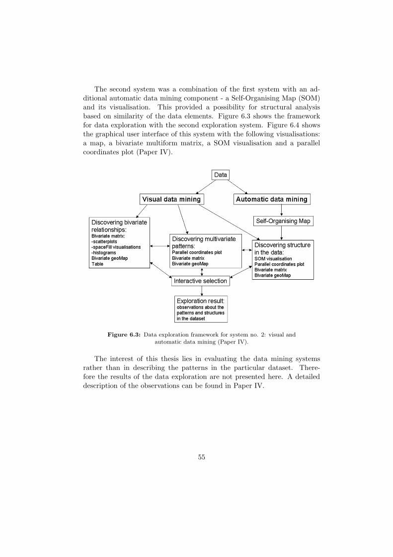
The second system was a combination of the first system with an ad-ditional automatic data mining component - a Self-Organising Map (SOM)and its visualisation. This provided a possibility for structural analysisbased on similarity of the data elements. Figure 6.3 shows the frameworkfor data exploration with the second exploration system. Figure 6.4 showsthe graphical user interface of this system with the following visualisations:a map, a bivariate multiform matrix, a SOM visualisation and a parallelcoordinates plot (Paper IV).

Figure 6.3: Data exploration framework for system no. 2: visual andautomatic data mining (Paper IV).

The interest of this thesis lies in evaluating the data mining systemsrather than in describing the patterns in the particular dataset. There-fore the results of the data exploration are not presented here. A detaileddescription of the observations can be found in Paper IV.

55

Fig

ure

6.4

:E

xplo

ring

radon

data

wit

hvisualand

auto

mati

cdata

min

ing

(Paper

IV).

56

6.3 Evaluation of the method

The visual data mining has proven to be useful in discovering bivariaterelationships in the radon dataset. The main goal was to find out if highconcentrations of radon were related to particular values of other variables.Another goal was to find patterns that could describe a relationship betweentwo variables, such as for example a decreasing or increasing dependency.For this purpose, the bivariate visualisations proved to be the most usefulones, as expected. Most of the patterns were observed in the scatterplotsand spaceFills. Some of the relationships could also be observed in thebivariate geoMap. The parallel coordinates plot was not very useful for thisexploration task and the table was not useful at all.

The parallel coordinates plot proved to be the best visualisation for dis-covering multivariate relationships. It was used to identify the primary cuesabout multivariate relationships, which were then further explored in othervisualisations, for example in the map when looking for spatial dependen-cies. The most interesting result was that a spatial cluster was identified inan area in Stockholm archipelago where high radon concentrations occur.This cluster was identified without any reference to the geographic locationof the data objects that belong to it, only by selecting a cluster of lines withparticular characteristics in the parallel coordinates plot. The geographiclocation of the objects in this cluster was only investigated at a later stage,when it was discovered that these objects were actually located in the samearea. This discovery of what the objects in this area have in common witheach other and where they differ from other objects lead to a hypothesis thatcould subsequently be used for further exploration. It should be pointed outthat without the parallel coordinates plot this cluster would not have beenidentified.

A combination of the visualisations and the SOM provided the possi-bility to see the structure in the data. The dataset was separated into sixclusters by the SOM. The integration of a computational method into theexploration system therefore proved useful for detecting the global structurein the datastet and a partition of the data in clusters. But only by usingthe SOM it was not possible to describe the characteristics of the clusters.It is a known fact that interpreting the internal knowledge representationof a neural network is not an easy task (Silipo 2003). The reasons for thisare that first, the knowledge is spread all over the weights and neurons ofthe SOM and second, that the knowledge representation might not havea physical meaning, because the network’s computation does not take intoaccount the physical meaning of the input variables. In this particular case,

57

however, the characteristics of each cluster could be described by observingthe clusters in other visualisations. This would not be possible if only theautomatic data mining method was used. The combination of visual andautomatic methods can therefore provide a way to interpret the result of theSOM, which raises the trust in the automatic method. This also makes theneural network look less like a black box with an unexplainable capabilityfor solving problems.

The most time consuming step in this case study was the pre-processingof the data into a suitable form for geoVISTA elements and in particularfor the geoMap. One downside of the geoMap is that it can only be usedfor area-based data. As the dataset of wells was a point dataset, it wastherefore necessary to convert it to some sort of area representation beforeit could be explored. At first 50m circular buffers were created around thewells. These proved to be too small for a good display in the map, soThiessen polygons were created instead. The visualisation of these provedto be adequate, but the disadvantage was that a very long processing timewas needed for their creation for such a large dataset. Another disadvantagewas that the polygons on the map did not correspond to any real objects.They were abstract representations of the wells, which can be confusing forthe explorer.

Another issue concerning the visualisation were the outliers. Ideally,when exploring a dataset with data mining, one should not remove any dataelements, as the outliers might contain hidden information about interestingpatterns. On the other hand, they might also be just products of mistakesor other uncertainties. In the case of radon data there were some very highoutliers, whose radon concentration was four times as large as the range ofall other values (63000 Bq/l as compared to the total range of 0-15000 Bq/l).Without removing these outliers, the range in some visualisations (in partic-ular in scatterplots and in the parallel coordinates plot) was stretched to thepoint that there was a significant amount of overprinting at small values andthe visualisations became unreadable at these values. Therefore the outliershad to be removed before the exploration, even though they might representcorrect measurements and indicate some interesting underlying pattern.

Observations that were made during the exploration may be relevant tothe problem of radon in groundwater. However, since the author is neither ageologist nor a geochemist, it was not possible to evaluate these observations.A discussion of the results with a radon expert was planned as a follow-upto this work, but was not carried out due to cirumstances beyond author’scontrol. One thing that should be pointed out is that the observationswere made with no previous knowledge about possible geological and other

58

dependencies between variables. They are therefore completely data-driven.From this point of view the integration of visual and automatic data miningapproach proved to be valuable for formulating hypotheses, as long as thediscovered patterns would be confirmed to be reasonable from the geologicaland geochemical point of view. A post-evaluation of the exploration resultsby an expert would therefore be crucial if the results were to be used infurther research.

59

Chapter 7

Case study 3 - spatio-visual data mining

for emergency response data

This chapter presents an attempt to explore emergency response data usinga spatio-visual data mining approach. The chapter is based on paper V.

The Fire and Rescue Services in the Helsinki Metropolitan area in Fin-land use a simple GIS-based model for risk analysis based on data aboutprevious incidents and other relevant information. The model uses simplespatio-statistical methods to identify risk zones from three variables, whichwere identified as the ones that have the strongest possible effect on riskoccurence (Karasova 2005). In reality, the occurence of fire and rescue in-cidents depends on many more factors. By trying to discover connectionsbetween other factors and the incidents, the model can be improved in or-der to assist the emergency preparedness planning and resource evaluation(Krisp and Karasova 2005).

In order to improve the risk model, two studies were performed at theInsitute of Cartography and Geoinformatics at the Helsinki University ofTechnology (HUT). One of them applied kernel density analysis and cross-tabulation to the incidents data in order to explore the strength of relation-ships between incidents and other factors (Krisp and Karasova 2005). Thesecond one used a spatial data mining approach with spatial associationrules in order to discover existing spatial relationships between the locationof fire and rescue incidents and specific geographic objects (Karasova 2005,Karasova et al. 2005). Based on these two studies and on the visual datamining study (Demsar 2004), an approach for exploring the incidents datawith a combination of spatial and visual data mining methods was developed(Paper V) in a collaboration between Helsinki University of Technology andthe Royal Institute of Technology in Stockholm.

7.1 The data and the exploration goal

The study area for the incidents data covered a 14x14km square area in thecentral part of Helsinki. It is shown in fig. 7.1. Exploration data consisted ofinformation about fire and rescue incidents, population information, a busi-ness register and information about topography and infrastructure. The goal

60

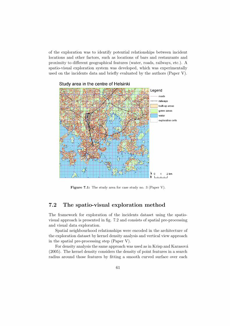
of the exploration was to identify potential relationships between incidentlocations and other factors, such as locations of bars and restaurants andproximity to different geographical features (water, roads, railways, etc.). Aspatio-visual exploration system was developed, which was experimentallyused on the incidents data and briefly evaluated by the authors (Paper V).

Figure 7.1: The study area for case study no. 3 (Paper V).

7.2 The spatio-visual exploration method

The framework for exploration of the incidents dataset using the spatio-visual approach is presented in fig. 7.2 and consists of spatial pre-processingand visual data exploration.

Spatial neighbourhood relationships were encoded in the architecture ofthe exploration dataset by kernel density analysis and vertical view approachin the spatial pre-processing step (Paper V).

For density analysis the same approach was used as in Krisp and Karasova(2005). The kernel density considers the density of point features in a searchradius around those features by fitting a smooth curved surface over each

61

Figure 7.2: Framework for the spatio-visual data mining (Paper V).

feature. The point feature is at the maximum point of the surface, whichdecreases with the distance from the feature until it reaches zero at the ker-nel radius. The surface can be any kind of smooth continuous fuction whichsatisfies this requirement. In this case, it was based on a quadratic function.A density raster is then produced by assigning to each cell a sum of all ker-nel surfaces which contain the centre of this cell (Krisp and Karasova 2005).The advantages of using densities are that they provide a good way of visu-alising a point pattern, visually indicate hot spots, are useful for detectingtrends and provide a good way to link point dataset to other geographicdatasets (O’Sullivan and Unwin 2003a).

The densities were integrated with other geographic layers by the verticalview approach from spatial data mining, similar to the one introduced byEstivill-Castro and Lee (2001). In order to be able to compare attributes fora particular location, density rasters were combined with other informationin a virtual overlay of all rasters into a table of cells and their respectiveraster values. Other information in the form of polygons or lines was trans-formed into proximity surfaces based on intersection. A cell in a proximitysurface was assigned value 1 if the feature in question intersected the celland 0 if the intersection was empty (Paper V).

The final exploration dataset consisted of 3136 polygons, where eachpolygon represented one raster cell of a 56x56 raster with 250m resolution,covering the study area. The dataset had 51 attributes, out of which 15 were

62

non-temporal and 36 were temporal. The temporal attributes consisted ofincident kernel densities according to time (daytime and night-time), type (6different types of incidents were considered) and year (2001-2003). All den-sities were produced with the same kernel and grid size. The non-temporalattributes included aggregated incident kernel densities and proximity sur-faces. Aggregated densities were produced for all night-time/daytime inci-dents and for all incidents over the whole time period 2001-2003. Proxim-ity surfaces were produced for each of the following features: water areas,built-up areas, railway network, railway stations and six different road types(Paper V).

The spatially pre-processed dataset was explored by visual data mining.Using different visualisations in combination with iteractive selection andbrushing, patterns and relationships could be discovered. These were dividedinto the following groups: bivariate patterns, multivariate patterns, spatialpatterns and temporal patterns. Additionally, the strength of the bivariaterelationships was visually estimated (Paper V).

The visual data mining system for exploration of the spatially prepareddataset was based on GeoVISTA Studio. The system was based on the de-sign of ESTAT (the Exploratory Spatio-Temporal Analysis Toolkit) (Robin-son et al. 2005) and had an additional multiform bivariate matrix (Mac-Eachren et al. 2003). The decision to build the system in this way was basedon the nature of the data. The temporal attributes in the dataset were thereason to include a time-series parallel coordinates plot as in ESTAT, whilethe goal to discover potential bivariate relationships between the incidentsand other attributes was the motivation for the multiform bivariate matrix.The graphical user interface of the system is shown in fig. 7.3 and has thefollowing visualisations: a time series parallel co-ordinates plot (TSPCP) ontop, a parallel coordinates plot (PCP) for non-temporal attributes in themiddle, a bivariate map and a multiform bivariate matrix with scatterplots,histograms and spaceFill visualisations (Paper V).

The exploration of the incidents dataset gave some interesting observa-tions, which are not described here. Rather, the thesis focuses on how thedata mining method performed. Some of the more interesting observationsabout the incidents dataset are presented in Paper V.

7.3 Evaluation of the method

The spatio-visual approach for exploration of incidents data is similar to thespatial data mining approach that applies classical data mining algorithms

63

Figure 7.3: The visual data mining system for the incidents dataset (PaperV).

to spatially pre-processed data. The difference is that, instead of a classicalmining algorithm, visual data mining was used. Since the design of thevisual data mining system included a special visualisation for time seriesattributes, temporal exploration of the data was also possible.

The pre-processing step is crucial when mining spatial data with eithertraditional mining algorithms or with visual data mining. It was typicallythe most time-consuming step of the exploration process. However, onceit was done, various algorithms could be applied to the prepared dataset.This has the advantage that if different mining algorithms are applied to thesame dataset, more patterns may be discovered than if only one algorithmwas used.

The pre-processing method also had some disadvantages. Since the den-sities were classified into several discrete values, a lot of overprinting was

64

present in some visualisations, in particular in the scatterplots and the par-allel coordinate plots. This could be avoided by using these visualisationsin combination with others where no overprinting occured.

Another disadvantage was that the spatial modelling using density anal-ysis and proximity surfaces depends on the resolution of the raster. Differentpatterns might therefore be discovered for rasters of different resolutions orrasters of the same resolution but at shifted positions. The densities are alsosensitive to the kernel radius and form of the kernel surface.

Temporal trends were best seen in the TSPCP and PCP in combinationwith the map. The map in combination with other visualisations was alsouseful for identification of spatial patterns and hotspots of incidents.

An unexpected result was that it was possible to visually estimate thestrength of bivariate relationships. This turned out to be useful in order toidentify the variables which are related to the incidents and could thereforebe included in the improved model for the risk analysis. However, since thesedependencies were the product of a visual estimation, they should first beconfirmed or rejected by using a computational model, such as for examplethe cross-tabulation suggested in Krisp and Karasova (2005).

Observations about the dataset could be used as the basis for hypothesesabout occurence of incidents. However, the findings should be evaluated bythe experts from the Finnish Fire and Rescue Services before they usingthem to improve the risk analysis model.

65

Chapter 8

Usability evaluation of the data mining

tools

8.1 User-centred design in geovisualiastion

Design of exploratory geovisualisation tools has been technology driven formany years. Tools and systems were developed from a purely technical pointof view, where knowledge about users did not play a major role. Only re-cently the attitude has changed towards user-centred design with the aimof providing useful and usable geovisualisation tools. Contemporary de-sign methods involve user participation through all steps of system design,from concept design through prototype development to final implementation(Fuhrmann et al. 2005).

User-centred design is a design approach for development of informa-tion systems where knowledge about the users is one of the main factorsin the system design process. It is the main concept of Human-ComputerInteraction (HCI), which is a discipline that explores how the quality of in-teraction between the users and information systems can be improved. Theuser-centred design considers not only technological, but also physiologicaland cognitive issues in order to create user-interfaces which support humansto make full use of their natural perceptive and cognitive skills (Preece etal. 2002, Haklay and Tobon 2003).

In HCI an information system is considered acceptable if it satisfies allthe needs and requirements of the users. Acceptability is subdivided intosocial acceptability and practical acceptability, which consists of usefulness,cost estimation, reliability and compatibility with other systems. Usefulnessaddresses the question if the system can accomplish the required task. It isfurther subdivided into utility, which questions if the system’s functionalityis able to do what it is supposed to do, and usability, which is concernedwith the ability of users to use that functionality. Usability is the extent towhich a computer system supports users to achieve specified goals in a givencontext of use and to do so effectively, efficiently and in a satisfactory way(Nielsen 1993). The model of system acceptability is presented in fig. 8.1.

Usability evaluation is the process of systematically collecting data onhow typical users use the system for a particular task in a particular type

66

Figure 8.1: A model of the system acceptability (redrawn after Nielsen(1993)).

of environment. It has three main goals: to assess the accessibility of thesystem’s functionality, to assess users’ experience of the interaction and toidentify any specific problems with the system (Nielsen 1993).

There are four main methodologies for performing a usability assessment:

• ’quick and dirty’ evaluation,

• usability testing,

• field studies and

• predictive evaluation.

A ’quick and dirty’ evaluation means that the users provide informal feed-back to the designers. Usability testing consists of two types of evaluation:formal methods, where quantitative data is collected on users’ performanceduring typical tasks, and exploratory usability, which investigates how usersuse the tools from the cognitive point of view. In field studies, the goal isto collect data on what users do in their natural environment and how tech-nology impacts their daily routines. In predictive evaluation, the experts areasked to predict how typical users would react to a particular usability issue(Hackos and Redish 1998, Preece et al. 2002, Dix et al. 2004).

The developers of exploratory visualisation systems have the task tomake the systems easy to learn and use. The ultimate goal is to make thecomputer vanish, as users become completely absorbed in their domains.This is not easy to accomplish. In these systems, the users may be knowl-edgeable in the problem domain but novices in the underlying computerconcepts. Their motivation is often high, but so are their expectations.

67

Usage can range from occasional to frequent. Tasks are more difficult todescribe, because of the exploratory nature of the applications. It is there-fore difficult to design and evaluate such systems (Shneiderman and Plaisant2005).

Whatever the application of the exploratory geovisualisation tools, itis essential to develop knowledge of whether the methods, tools and solu-tions that are produced, actually work and can be used for the task theyare meant for. In order to strive towards this goal, it is useful to borrowand adapt methods from usability engineering in HCI. Testing usability forgeovisualisation systems is dominated by cognitive issues, such as attention,perception, memory, problem solving, hypothesis generation and decisionmaking. The key question is whether geovisualisation systems are effectivefor spatial problem solving. This requires investigation methods that go be-yond the traditional usability evaluation methods (Tobon 2002, Fuhrmannet al. 2005, Swienty 2005).

Attempts on usability research in geovisualisation can be divided intotwo main types, mainly formal usability evaluations and some individualexploratory usability attempts (Fuhrmann et al. 2005). Formal evaluationmethods measure the typical users performance on carefully prepared tasks.Data collected in a formal usability session is observational and consists ofcontrolled measurements of the number of errors and time to complete thetask. Data on user satisfaction is also typically collected in questionnairesand interviews. Exploratory usability on the other hand is not concernedwith users performance, but principally investigates how users use the toolsand the cognitive processes during the testing. It produces descriptive datain the form of verbal protocols and observational notes (Preece et al. 2002,Griffin 2004).

Formal and exploratory usability evaluation methods complement eachother. Rather than conducting only controlled experiments or observing onlynaturalistic situations, both approaches should be used to better understandhow the exploration process evolves. An analogy for this combination of re-search methods can be found in the research practices in other fields, forexample, in biology. In biological research, scientists use ”in vitro” meth-ods to investigate an organism in controlled laboratory settings. In parallelthey observe how the same organism behaves ”in vivo”, in its natural envi-ronment. Using both approaches in parallel helps to build a more completemodel about a particular organism. An analogy to the ”in vitro/in vivo” ap-proach in usability research is a combination of both formal and exploratoryusability (Dunbar 2001, Griffin 2004).

Some recent examples of user studies and usability testing in geovisu-

68

alisation include a formal evaluation of five different interactive tools forexploratory analysis of geographically referenced data (Andrienko N et al.2002) and testing of the suitability of coupling an aspatial visualisation sys-tem with a GIS system (Tobon 2002). Haklay and Tobon (2003) evaluateda Public Participation GIS (PPGIS) for environmental planning. Griffin(2004) presented an exploratory usability evaluation of data display de-vices for geographical models. Ahonen-Rainio (2005) conducted user testsof metadata visualisation by performing concept tests for user requirementsand a prototype test. Koua (2005) performed a formal usability evaluationof an integrated exploration system, where various geospatial visualisationswere combined with a Self-Organising Map. Several tools based on Geo-VISTA studio have also been subject to usability evaluation, including ausability experiment for a geovisualisation system for health statistics (Ed-sall 2003b) and a report on how ESTAT - an exploratory geovisualisationtoolkit for epidemiology, based on GeoVISTA, was designed using the user-centred development process (Robinson et al. 2005).

8.2 Usability evaluation in case study 1

The user-centred approach was an integral part of the design of INVISIPtools. Users were involved in the project throughout the development, fromdefining the requirements to the evaluation of the final demonstrator soft-ware. Tests were scheduled during several stages of the process and per-formed for different systems developed within INVISIP (Limbach 2002).

The Visual Metadata Browser - VisMeB was the tool where the user-centred design approach was followed most faithfully. This tool was evalu-ated several times during the design process by the following methods:

• formal user tests with paper mock-ups, HTML and java prototypes,

• focus groups,

• interviews,

• web-based questionnaires and

• a heuristics evaluation with experts.

Results of these evaluations were presented by Jetter (2003), Bey (2004),Gerken (2004) and Klein (2005).

69

The prototypes for GeoLibrary and the metadata Entry tool were eval-uated during a formal evaluation at the same time as the VisMeB (Limbach2003).

An evaluation of the VDM tool, which is relevant to this thesis, wasconducted simultaneously with the formal evaluations for the other IN-VISIP tools. The participants in this evaluation were users from the IN-VISP project, who were not involved in the development of the VDM tool.Test participants were asked to complete certain tasks with the VDM tool(Hauska 2005). The author of this thesis was a developer of the VDMtool and therefore could not participate in the evaluation as a test person.According to recent communication from the INVISIP partner who was re-sponsible for this testing, no results about the VDM tool were ever publishedanywhere.

8.3 Usability evaluation in case study 2

Case study no. 2, where a combination of visual and automatic data miningwas applied to environmental research, was from the very beginning plannedaccording to the principles of the user-centred design. The first step in thedesign was a learning process about a particular issue to be solved (i.e. aboutradon in groundwater). As the author of this thesis is not a geologist or ageochemist, a participation observation approach was adopted in order to getacquainted with the exploration problem. Over a period of several months,the author worked together with Kirlna Skeppstrom, a PhD student from theLand and Water Engineering Department at the Royal Institute of Technol-ogy, who is an expert for the problem of radon in groundwater. Skeppstrom(2005) recently published a licenciate thesis on ’Radon in Groundwater - In-fluencing Factors and Prediction Methodology for a Swedish Environment’.The goal of the cooperation was to identify a data exploration problem re-lated to radon in groundwater that could be approached by a combinationof visual and automatic data mining. Several different methods of visualexploration were tried. One of them demosntrated how three-dimensionalthematic surfaces can be used for discovery of radon-related spatial patterns(Demsar and Skeppstrom 2005). The learning process consisted of frequentsemi-formal sessions and ”quick and dirty” evaluations by email or phone.

After the exploration systems were developed (Paper IV), a prototypeevaluation was planned. The experiment was intended to address two goals.The first goal was to perform a formal usability evaluation of the toolsin order to test how successfully various visualisation operations can be

70

performed. The second goal was to identify the differences between userswith different backgrounds. An exploratory usability session was planned,where GIS experts and environmental experts were to be observed whileworking with the systems. The intention was to observe the explorationstrategies adopted with people with different academic backgrounds anddifferent experiences with GIS.

The final stage of the user-centred design in case study 2 was to be afield study with Mrs. Skeppstrom. The goal was to investigate if the combi-nation of visual and automatic data mining could echo the results obtainedfrom a structured statistical analysis. Mrs. Skeppstrom would have beenasked as the expert for radon in groundwater to visually explore the samedata she had previously analysed statistically and try to see if she could findsupport for her previously derived conclusions. The goal of this experimentwas to investigate if a visual system could be relied upon for exploratorytasks in environmental analysis. Most of the environmental scientists thatthe author was in contact with possess a certain skepticism towards visual-isation techniques for data exploration and are suspicious about their use.There seems to exist a consensus among environmental scientists that var-ious aspects of the data may be misrepresented if one were to rely solelyon visual exploration methods. The experiment was therefore planned tocompare visual and statistical methods on the same dataset. The aim wasto demonstrate that visualisation can be useful for the hypothesis formingprocess and can complement traditional statistical methods.

Due to external circumstances beyond author’s control, the prototypeevaluation and the field study could not be carried out.

8.4 Usability evaluation in case study 3

The exploration system from the case study 3 (Paper V) was evaluated usinga combination of a formal evaluation and exploratory usability assessment(Paper VI). This section presents the experiment and summarizes the re-sults. Details about the design, the participants and the execution of theexperiment are described in Paper VI.

The objective of the formal evaluation was to evaluate users’ perfor-mance on pre-defined exploration tasks. During the exploratory part of theexperiment, data were collected on what hypotheses the users form and inwhat way they construct new knowledge. The participants were allowed toexplore data freely during this stage. The test combined the two complemen-tary approaches, the quantitative and the qualitative, in order to attempt

71

to assess the usability of a visual data mining system in as complete a wayas possible.

The test was performed with limited resources regarding the cost andtesting personnel. Therefore it has been designed in a way that allowedto gather the maximum amount of information with the minimum possi-ble means. Simple data capture techniques were used instead of expensivemethods. Another provision to stay within available resources was to use theminimal possible number of participants - two for the pilot study and fourfor the real testing. This number may seem small, but it has been shownthat the maximum ratio between the benefit and the cost in terms of timeand effort for testing has been achieved when using three to five participants(Nielsen 1994). The test participants were postgraduate students, teachersand researchers at the Royal Institute of Technology in Stockholm. Threeparticipants had their academic background in surveying engineering, two innatural sciences and one in computer science. They had a varied experiencewith GIS, from no experience to over 10 years’ experience. They were notnative English speakers, but they all possessed a good knowledge of English,which was the language of the test.

8.4.1 Formal evaluation

The process of exploring geospatial data can be subdivided into tasks, suchas identifying spatial positions of objects, identifying their spatial distribu-tion and density, analysing proximity, etc. These tasks can be performedusing a number of visualisation operations (Koua 2005).

For the formal evaluation part of the experiment a selection of explo-rational tasks has been designed, based on a typical visualisation opera-tions. Considering the practical limitations of this testing, a set of threevisualisation operations was selected from a larger taxonomy (Wehrend andLewis 1990). The selection was based on the relevancy of the operationsto the exploration of incidents dataset. The primary goal of exploring thedataset was to identify spatial patterns related to various types of incidents.Relationships between attributes should also be identified. In order to ful-fill these two goals, the following three visualisation operations were foundto be the most relevant ones: associate, compare and describe the spatialdistribution. The compare operation was further subdivided into spatiallycompare, where the goal was to compare values of objects or data elements atdifferent spatial locations and compare, where values of different attributeshad to be compared at the same location. Each of these four selected visu-alisation operations was tested by asking the participants to complete two

72

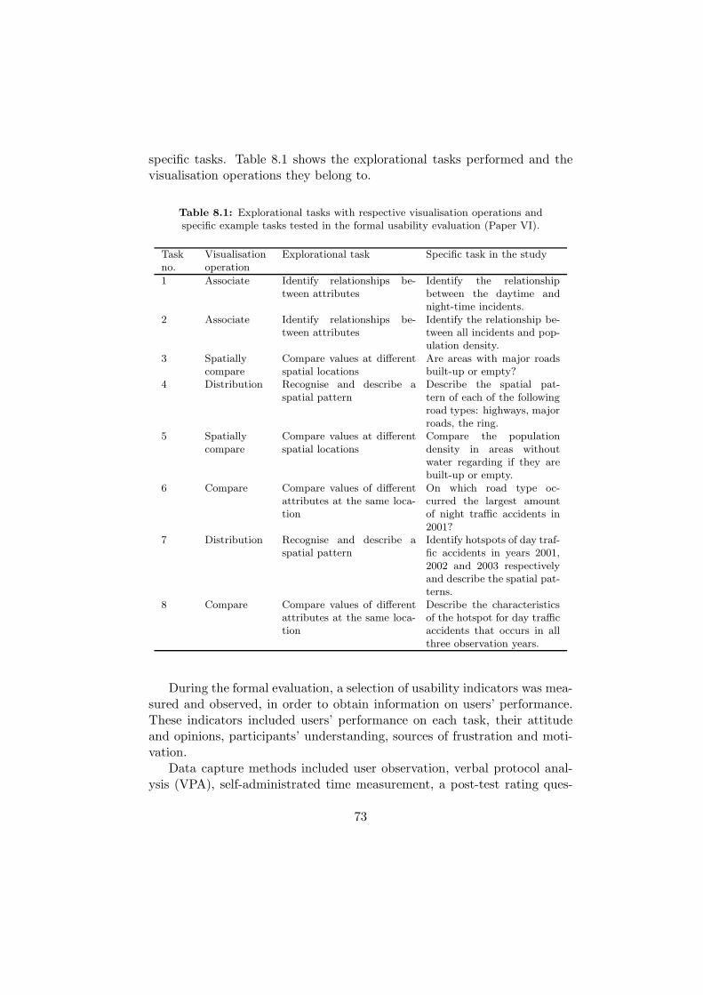
specific tasks. Table 8.1 shows the explorational tasks performed and thevisualisation operations they belong to.

Table 8.1: Explorational tasks with respective visualisation operations andspecific example tasks tested in the formal usability evaluation (Paper VI).

Taskno.

Visualisationoperation

Explorational task Specific task in the study

1 Associate Identify relationships be-tween attributes

Identify the relationshipbetween the daytime andnight-time incidents.

2 Associate Identify relationships be-tween attributes

Identify the relationship be-tween all incidents and pop-ulation density.

3 Spatiallycompare

Compare values at differentspatial locations

Are areas with major roadsbuilt-up or empty?

4 Distribution Recognise and describe aspatial pattern

Describe the spatial pat-tern of each of the followingroad types: highways, majorroads, the ring.

5 Spatiallycompare

Compare values at differentspatial locations

Compare the populationdensity in areas withoutwater regarding if they arebuilt-up or empty.

6 Compare Compare values of differentattributes at the same loca-tion

On which road type oc-curred the largest amountof night traffic accidents in2001?

7 Distribution Recognise and describe aspatial pattern

Identify hotspots of day traf-fic accidents in years 2001,2002 and 2003 respectivelyand describe the spatial pat-terns.

8 Compare Compare values of differentattributes at the same loca-tion

Describe the characteristicsof the hotspot for day trafficaccidents that occurs in allthree observation years.

During the formal evaluation, a selection of usability indicators was mea-sured and observed, in order to obtain information on users’ performance.These indicators included users’ performance on each task, their attitudeand opinions, participants’ understanding, sources of frustration and moti-vation.

Data capture methods included user observation, verbal protocol anal-ysis (VPA), self-administrated time measurement, a post-test rating ques-

73

tionnaire and a survey. User observation involves watching and listeningto users during the interaction with system in order to identify how theyare supported by the system (Preece et al. 2002). Verbal protocol analysis(VPA) or the thinking-aloud protocol requires users to say out loud every-thing that they are thinking and trying to do and in this way externalisetheir thought processes. Verbalisations make it possible to understand notonly what problems the participants have, but also why these problemsarise. VPA is also an efficient way for performing a low-cost usability ex-periment, because it produces a lot of information from a few participants(Jordan 1998). Another measure for a low-cost experiment was to use self-administered time measurements, where the users were required to writedown the times they used for each task (Nielsen 2000). After the test theparticipants filled in a rating questionnaire, where they had to mark on apredefined scale their opinion about particular visualisations and the sys-tem. This questionnaire was designed to measure the perceived usefulness,ease of use and satisfaction with the system. Finally the participants hadto complete a survey that consisted of open-ended questions (Jordan 1998).

From the visualisation operations, all the participants successfully com-pleted the two tasks for the operation spatially compare. Performance wasslightly less successful for operations distribution and compare, where themajority of the participants completed the tasks. The operation associatehad the least successful performance, where in one of the two tasks nobodyidentified the target answer.

Measuring the performance time was not very useful. One reason for thisis that due to limited resources it was not possible to arrange precise timemeasurements. Another reason is that the visual data mining concept andthe way the geoVISTA-based system works were new to all participants.Some of them frequently needed to recheck in the instructions how theycould use a particular visualisation. Therefore the task time includes thetime spent for searching for help in the instructions and does not reflect thetask performance very well.

When it comes to evaluation of particular visualisations, contrary to ex-pectations most of the participants found the multiform bivariate matrix tobe a difficult method to use. Controversially, this was a visualisation, withthe concept of which they were familiar from before and which also receivedthe highest ratings in the rating questionnaire. This finding is similar tothe one by Ahonen-Rainio (2005), who tested a scatterplot matrix for ex-ploration of geographical metadata. The scatterplot matrix was considereda very complex method by her participants. Ahonen-Rainio reasoned thatthough each scatterplot is simple to read as such, once they are arranged in

74

a more complex structure, they become difficult to use for non-trained per-sons. This is a valid argument also for a bivariate multiform matrix, whichis even more complex than a scatterplot matrix, as it includes a visualisationthat the participants were not familiar with beforehand - the SpaceFill.

The other three visualisations, the map, the PCP and the TSPCP re-ceived opinions and ratings as expected. The map was relatively easy tounderstand and use, even though it had some disadvantages, such as thelack of ability to show several geographic layers and to display point and linedata. The PCP and TSPCP were very confusing in the beginning, but oncethe participants grasped the general idea about how these visualisations areconstructed, they used them enthusiastically and without significant prob-lems.

8.4.2 Exploratory usability

The second objective of the usability assessment was to try to understandhow users explore geospatial data and what exploration strategies theyadopt. In spite of some recent attempts to understand the way users exploregeospatial data (Tobon 2002, Griffin 2004), we do not know very much aboutit. The goal of the exploratory usability experiment was to observe whatexploration strategies do the participants develop when freely using the sys-tem. In order to achieve this goal, the participants were given free hand toperform whatever exploration they wished in any way they wanted duringa limited amount of time. They were asked to verbalise their thoughts, i.e.”think aloud”, so that the observer could keep a verbal protocol. The pro-tocols were analysed with respect to the hypotheses the participants formedand the way they did that. The results were compared with the internalmodel of the visualisation process by Tobon (2002), presented in fig. 8.2.

It was found that the participants followed two distinct cognitive strate-gies in data exploration. Half of them repeatedly went through the followingsteps: first they formed a hypothesis, which was based on their backgroundknowledge. Then they looked at and interactively manipulated visualisa-tions trying to gather evidence for or against the hypothesis. They inter-preted the results, until they could evaluate the initial idea. Once they didthis, they discarded this particular hypothesis and started from scratch, byforming another, completely unrelated hypothesis, which was again basedonly on their background knowledge. They did not systematically explorethe data, i.e., go through all the available attribute values or attributes,but checked various visualisations rather at random. They have not com-pleted the whole circle through the exploration visualisation process, but

75

Figure 8.2: The internal model of the visualisation exploration process assuggested by Tobon (2002).

repetitively followed a loop-like path, shown in fig. 8.3.The second half of the participants formed the initial hypothesis based

on what they saw in the system. They systematically checked all availableattributes or all available attribute values. They interpreted the findings,adapted the original hypothesis and decided where to look next based onwhat they discovered. This systematical exploration was repeated severaltimes, always adapting and improving the initial hypothesis and not jumpingto something completely different as the first group of participants did. Thisexploration strategy followed the circle in Tobons exploration model and ispresented in fig. 8.4.

The distinction in the way that the two groups of participants exploredthe data might indicate that investigating data visually with the aim toform a hypothesis is not simple. A similar finding was presented by Tobon(2002), who reasoned that although humans might be good at visual pat-tern recognition, they need to understand and decode information from thegraphic display. The reason that the first group of participants did not basetheir hypotheses on what they saw, might be that they subconscioulsy con-sidered the visualisations to be too complex. This indicates that if the level

76

Figure 8.3: The exploration strategy of the first group of participants.

of complexity is too advanced, it might be difficult for certain individualsto translate what they see in a visualisation into a meaningful hypothesisabout the data.

The data for the exploratory usability experiment was collected by thethinking-aloud method. One of the known disadvantages of this method isthat the participants are required to perform two tasks at the same time:besides using the system, they are trying to describe what they are doing.For some individuals, these might be very difficult tasks to perform simulta-neously. This was also confirmed here, as thinking-aloud varied very muchbetween the participants. Some of the participants fluently verbalised theirthoughts, while others fell completely silent at times. One of the reasonsfor this is probably the use of English in this study. English was not thenative language of any of the participants, even though all of them speakit fluently. Their communicability in the thinking-aloud process might havebeen different if they had a chance to verbalise their thoughts in their nativelanguages. Even better results could be expected if the whole test as wellas the user interface was in the native language of each participant, as itis indicated by the tests performed by Andrienko N et al. (2002). In thisstudy this was not possible to implement due to the cultural heterogeneity

77

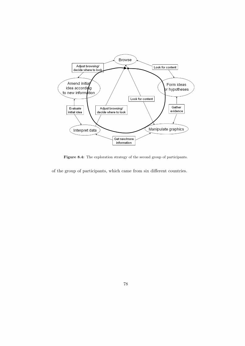
Figure 8.4: The exploration strategy of the second group of participants.

of the group of participants, which came from six different countries.

78

Chapter 9

Conclusions

9.1 Summary of the results

The thesis presented three different applications of a combination of auto-matic and visual data mining for geospatial data. The three case studiesidentified three possible application areas: exploring geographic metadatafor site planning, exploring a large environmental database and investigat-ing emergency response data. Although this exploration approach has itsstrengths and weaknesses, it was found to be useful in all three applicationareas. The main goal of the thesis - to investigate if a combination of auto-matic and visual data mining is a suitable approach for exploring geospatialdata - has been thereby achieved. In all three application cases, the com-bination approach for the exploration of the geospatial data proved to bevaluable for detecting patterns and observations, which could serve as thebasis for hypotheses about the dataset.

The approach was successful for discovering different types of patternsand structures in the data: bivariate relationships, multivariate relationshipsand underlying structure in the data. In one case it was also useful forestimating the strength of the bivariate relationships. Table 9.1 shows anoverview of the patterns that were identified and the method that was usedfor their identification.

Table 9.1: Identified patterns and methods that lead to their identification.

Identified pattern Identification methodVisual data mining Automatic data mining

bivariate relationships Xstrength of bivariate relationships Xmultivariate relationships X Xdata structure Xcharacterisation of data structure X Xsimilarity of data elements X

Visual data mining was used to discover bivariate relationships, estimatetheir strength and identify multivariate relationships. Automatic methods

79

were necessary to identify the underlying structure in the data and to in-vestigate similarity of the data elements. The structure in the data couldnot be described without the integration of the automatic method with thevisualisations. The visualisations provided the possibility to describe char-acteristics of each structural element (cluster) and the spatial pattern ofthese elements. This would not have been possible if only automatic miningwas used.

Another advantage of the combined approach was that the visualisa-tions provided a nice way to show and explain the results of the complicatedcomputational mining. The discovered knowledge was expressed in an in-tuitively understandable way through visualisation. In this way, results ofthe mining could easily be presented to the general audience, as there is norequirement to understand difficult algorithms or other procedures.

A disadvantage of the combined exploration system is that even thoughthe method proved to be adequate to preliminary identify the patterns inthe data, there was no possibility provided to evaluate the significance ofobservations. The method is therefore useful in the first step of data ex-ploration and helps forming preliminary ideas and hypotheses, but furtherinvestigation is needed to value the findings. An evaluation by a domain ex-pert is crucial before the observations could serve as hypotheses for furtherresearch.

The combined automatic-visual approach also has the disadvantage thatits concept is very novel to most of the potential users. In the usability eval-uation of the system in case study no. 3, the participants were chosen fromacademia and were all but one experienced users in terms of working withgeospatial data and GIS. Therefore it was expected that they should nothave too many difficulties operating the system and might even be consid-ered too experienced to detect the basic problems. It turned out that theywere in principle able to understand and adopt the new ideas of visually ex-ploring geospatial data. However, the concept of visual data mining, unusualvisualisations and interactive exploration was so novel to most of them thateven these experienced GIS users needed an extensive introductory training.Some of the visualisations, such as the spaceFill and the parallel coordinatesplot were also previously unknown to most of the participants and weresources of frustration on the users’ side. Training is therefore essential inorder to make use of all the benefits of the combined automatic and visualexploration approach. For a trained explorer it is, however, quite easy toidentify relationships and patterns in the visualisations.

One of the most interesting experiments in this thesis was the exploratoryusability evaluation of the system in case study no. 3. This evaluation in-

80

dicated that while different users explore geospatial data in different ways,there possibly exists an underlying mechanism on how the internal visualisa-tion model evolves. The study also indicated that investigating data visuallyis not simple. Although humans are good at visual pattern recognition, itis difficult for certain individuals to translate the observed pattern into ameaningful hypothesis. What this depends upon and which factors dictatehow the visualisation process develops in each individual, is not possible tosay after such a limited experiment as this study. But it is very interestingand can be an idea for further research.

9.2 Needs for further research

Based on the literature survey of spatial and visual data mining there areat the moment only very few attempts to combine real spatial mining withvisual exploration in the sense of integrating a visualisation of a spatiallyaware data mining algorithm with other visualisations. Combining spatialand visual mining is therefore a research goal for the future.

How geovisualisation tools help scientists think is as yet an unexploredtopic. Larger experiments are required to observer how cognitive thinkingmodels evolve. As the key point in data exploration is the intuitive searchprocess in a visualised environment, it is necessary to include physiologicaland psychological findings about the process of human vision as well asknowledge of the relation between geospatial objects and their representationin the human memory in the system engineering.

An imporant issue to investigate in the development of exploratory geo-visualisation tools is how humans perceive and interpret visual properties.Performing certain explorational tasks in a visual system requires more cog-nitive processing than others, depending on the complexity of the visual-isation. The ability to understand what the visualisation shows and tointepret the perceived pattern into a meaningful hypothesis differs betweenindividuals. The development of exploratory systems should therefore bebased not only on data mining and geovisualisation theories but also onfindings from cognitive and neurological sciences, such as theories about vi-sual perception of graphic variables and animation, psychological laws ofvisual acuity, figure-ground relationships, physiological findings about eyemovements, processing of information in the brain, memory mechanisms,etc. This could help the geovisualisation scientists to create user-interfaceswhich would support humans to make full use of their natural cognitiveskills.

81

Another interesting issue is how users with different backgrounds formhypotheses and construct knowledge when working with exploratory geovi-sualisation systems. One of the findings in the usability experiment indicatedthat there are substantial inter-individual differences in forming cognitive ex-ploration strategies. These differences might be related to users’ backgroundand domain knowledge. An interesting question to explore would thereforebe how the cognitive thinking process differs in different types of people andhow it is related to previous experience. The answer to this question couldassist the developers to design systems which would be optimally adaptedfor a particular group of users. These exploratory systems could then act asa communication, interaction and shared memory tool between a group oftarget users.

82

References

ADL - Alexandria Digital Library (2004) University of California at Santa Barbara.http://www.alexandria.ucsb.edu/research/ (accessed 1 Feb 2006).

ADEPT - Alexandria Digital Earth Prototype - Digital Earth (2004) University of Cali-fornia at Santa Barbara. http://www.alexandria.ucsb.edu/research/de/ (accessed1 Feb 2006).

Ahonen-Rainio P (2005) Visualization of geospatial metadata for selecting geographicdatasets. PhD thesis, Helsinki University of Technology, Helsinki, Finland.

Ancona D, Freeston M, Smith T and Fabrikant S (2002) Visual Explorations for theAlexandria Digital Earth Prototype. In: Goos G, Hartmanis J and van LeeuwenJ (eds) Visual Interfaces to Digital Libraries, Lecture Notes in Computer Science,2539:199-213. Springer Verlag, Berlin-Heidelberg.

Andersen D, Carver L, Dolin R, Fischer C, Frew J, Goodchild M, Ibarra O, Kothuri R,Larsgaard M, Manjunath B, Nebert D, Simpson J, Smith T, Yang T and Zheng Q(1995) The WWW Prototype of the Alexandria Digital Library. In: Proceedings ofthe International Symposium on Digital Libraries. Tsukuba, Japan.

Anderson T, Hussam A, Plummer B and Jacobs N (2002) Pie Charts for VisualizingQuery Term Frequency in Search Results. In: Lim E-P, Foo S, Khoo C, ChenH, Fox E, Urs S and Costantino T (eds) Digital Libraries: People, Knowledge,and Technology: 5th International Conference on Asian Digital Libraries, ICADL2002, Lecture Notes in Computer Science, 2555:440-451. Springer Verlag, Berlin-Heidelberg.

Andrienko N, Andrienko G, Voss H, Bernardo F, Hipolito J and Kretchmer U (2002)Testing the Usability of Interactive Maps in CommonGIS. Cartography and Geo-graphic Information Science, 29(4):325-342.

Andrienko G, Andrienko N and Voss H (2003a) GIS for everyone: the CommonGISproject and beyond. In: Peterson M (ed) Maps and the Internet, 131-146. ElsevierScience.

Andrienko G, Andrienko N and Gitis V (2003b) Interactive maps for visual explorationof grid and vector geodata. ISPRS Journal of Photogrammetry & Remote Sensing,57:380-389.

Andrienko N, Andrienko G and Gatalsky P (2003) Exploratory spatio-temporal visual-ization: an analytical review. Journal of Visual Languages and Computing, 14:503-541.

Andrienko G, Andrienko N and Gatalsky P (2004) Visual Mining of Spatial Time SeriesData. In: Proceedings of the 8th European Conference on Principles and Practiceof Knowledge Discovery in Databases, PKDD 2004, Lecture Notes in ComputerScience, 3202:524-527. Springer Verlag, Berlin-Heidelberg.

Andrienko N and Andrienko G (2006) Exploratory Analysis of Spatial and TemporalData. Springer Verlag, Berlin-Heidelberg.

Ankerst M (2000) Visual Data Mining. PhD thesis, Ludwig-Maximilians-Universitat,Munchen, Germany.

83

Beaubouef T, Ladner R and Petry F (2004) Rough Set Spatial Data Modelling for DataMining. International Journal of Intelligent Systems, 19:567-584.

Bederson BB, Shneiderman B and Wattenberg M (2002) Ordered and Quantum Treemaps:Making Effective Use of 2D Space to Display Hierarchies. ACM Transactions onGraphics (TOG), 21(4):833-854.

Bey A (2004) Der CircleSegmentView: Design und Evaluation einer Query Preview.Bachelor thesis, University of Konstanz, Konstanz, Germany.

Borgman CL, Leazer GL, Gilliland-Swetland AJ, Gazan R (2001) Iterative Design andEvaluation of a Geographic Digital Library for University Students: A Case Studyof the Alexandria Digital Earth Prototype (ADEPT). In: Constantopoulos P andSølvberg IT (eds) European Conference on Research and Advanced Technology forDigital Libraries, ECDL 2001, Lecture Notes in Computer Science, 2163:390-401.Springer Verlag, Berlin-Heidelberg.

Buono P and Costabile MF (2005) Visualizing Association Rules in a Framework forVisual Data Mining. In: Hemmje M, Niederee C and Risse T (eds) From Inte-grated Publication and Information Systems to Information and Knowledge En-vironments, Lecture Notes in Computer Science, 3379:221-231. Springer Verlag,Berlin-Heidelberg.

Chawla S, Shekhar S, Wu W and Ozesmi U (2001) Modelling spatial dependencies formining geospatial data. In: Miller HJ and Han J (eds) Geographic Data Miningand Knowledge Discovery, 131-159. Taylor & Francis, London and New York.

Chittaro L, Combi C and Trapasso G (2003) Data mining on temporal data: a visualapproach and its clinical application to hemodialysis. Journal of Visual Languagesand Computing, 14:591-620.

Coleman AS, Smith TR, Buchel OA and Mayer RE (2001) Learning Spaces in DigitalLibraries. In: Constantopoulos P and Sølvberg IT (eds) European Conference onResearch and Advanced Technology for Digital Libraries, ECDL 2001, Lecture Notesin Computer Science, 2163:251-262. Springer Verlag, Berlin-Heidelberg.

Cox KC, Eick SG and Wills GJ (1997) Brief Application Description - Visual Data Min-ing: Recognizing Telephone Calling Fraud. Data Mining and Knowledge Discovery,1:225-231.

Darby S, Hill D, Auvinen A, Barros-Dios JM, Baysson H, Bochicchio F, Deo H, Falk R,Forastiere F, Hakama M, Heid I, Keienbrock L, Kreuzer M, Lagarde F, MakelainenI, Muirhead C, Oberaigner W, Pershagen G, Ruano-Ravina A, Ruosteenoja E,Schaffrath Rosario A, Tirmarche M, Tomasek L, Whitley E, Wichmann HE andDoll R (2005) Radon in homes and risk of lung cancer: collaborative analysis ofindividual data from 13 European case-control studies. British Medical Journal,330:223-228.

Demsar U (2004) Exploring geographical metadata by automatic and visual data mining.Licenciate thesis, Royal Institute of Technology (KTH), Stockholm, Sweden.

Demsar U and Skeppstrom K (2005) Use of GIS and 3D visualisation to investigateradon problem in groundwater. In: Hauska H and Tveite H (eds) Proceedings of thethe 10th Scandinavian Research Conference on Geographical Information Science,ScanGIS2005, 39-51. Stockholm, Sweden.

84

Dix A, Finlay J, Abowd GD and Beale R (2004) Human-Computer Interaction, 3rd

edition, ch. 9: Evaluation techniques, 318-364. Pearson-Prentice Hall, Harlow,England, UK.

Dunbar K (2001) What Scientific Thinking Reveals About the Nature of Cognition. In:Crowley K, Shunn CD and Okada T (eds) Designing for Science - Implicationsfrom Everyday, Classroom and Professional Settings, 115-140. Lawrence ErlbaumAssociates Publishers, Mahwah, New Jersey, USA.

Dykes JA and Mountain DM (2003) Seeking structure in records of spatio-temporalbehaviour: visualization issues, efforts and applications. Computational Statistics& Data Analysis, 43:581-603.

Dykes J, MacEachren AM and Kraak M-J (2005) Exploring Geovisualization. In: DykesJ, MacEachren AM and Kraak M-J (eds) Exploring Geovisualization, 3-19. Elsevierand International Cartographic Association (ICA), Oxford, UK.

Edsall RM (2003a) The parallel coordinates plot in action: design and use for geographicvisualization. Computational Statistics & Data Analysis, 43:605-619.

Edsall RM (2003b) Design and Usability of an Enhanced Geographic Information Systemfor Exploration of Multivariate Health Statistics. The Professional Geographer,55(2):146-160.

Ester M, Frommelt A, Kriegel H-P and Sander J (2000) Spatial Data Mining: DatabasePrimitives, Algorithms and Efficient DMBS Support. Data Mining and KnowledgeDiscovery 4:193-216.

Estivill-Castro V and Lee I (2001) Data Mining Techniques for Autonomous Explorationof Large Volumes of Geo-referenced Crime Data. In: Proceedings of the 6th Inter-national Conference on Geocomputation. Brisbane, Australia.

Fayyad U and Grinstein GG (2002), Introduction. in: Fayyad U, Grinstein GG andWierse A (eds) Information Visualisation in Data Mining and Knowledge Discov-ery, 1-17. Morgan Kaufmann Publishers, San Francisco, USA.

Fotheringham AS (1999) Trends in quantitative methods III: stressing the visual. Progressin Human Geography, 23:597-606.

Fotheringham AS, Brunsdon C and Charlton M (2000) Quantitative Geography - Per-spectives on Spatial Data Analysis. SAGE Publications, London, UK.

Freitas AA (2002) Data Mining and Knowledge Discovery with Evolutionary Algorithms.Springer Verlag, Berlin-Heidelberg.

Fuhrmann S, Ahonen-Rainio P, Edsall RM, Fabrikant SI, Koua EL, Tobon C, WareC and Wilson S (2005) Making Useful and Useable Geovisualization: Design andEvaluation Issues. In: Dykes J, MacEachren AM and Kraak M-J (eds) Explor-ing Geovisualization, 553-566. Elsevier and International Cartographic Association(ICA), Oxford, UK.

Gahegan M, Takatsuka M, Wheeler M and Hardisty F (2002) Introducing Geo-VISTAStudio: an integrated suite of visualization and computational methods for explo-ration and knowledge construction in geography. Computers, Environment andUrban Systems, 26:267-292.

Gerken J (2004) Evaluation eines Metadatenbrowsers Liste vs. Leveltable. Bachelorthesis, University of Konstanz, Konstanz, Germany.

85

Ghosh J (2003) Scalable Clustering. In: Ye N (ed) The Handbook of Data Mining,247-278. Lawrence Erlbaum Associates Publishers, Mahwah, New Jersey, USA.

Gobel S and Jasnoch U (2001) Visualization techniques in metadata information systemsfor geospatial data. Advances in Environmental Research, 5(4):415-424.

Gobel S, Haist J, Reiterer H and Muller F (2002) INVISIP: Usage of InformationVisualization Techniques to Access Geospatial Data Archives. In: Cicchetti R,Hameurlain A and Traunmuller R (eds) 13th International Conference on Databaseand Expert Systems Applications, DEXA 2002, Lecture Notes in Computer Science,2453:371-380. Springer Verlag, Berlin-Heidelberg.

Griffin A (2004) Understanding how scientists use data-display devices for interactivevisual computing with geographical models. PhD thesis, The Pennsylvania StateUniversity, Pennsylvania, USA.

Grinstein GG and Ward MO (2002) Introduction to Data Visualization. In: Fayyad U,Grinstein GG and Wierse A (eds) Information Visualisation in Data Mining andKnowledge Discovery, 21-45. Morgan Kaufmann Publishers, San Francisco, USA.

Grunfeld K (2005) Visualization, integration and analysis of multi-element geochemicaldata. PhD thesis, Royal Institute of Technology (KTH), Stockholm, Sweden.

Guo D, Gahegan M, MacEachren AM and Zhou B (2005) Multivariate Analysis andGeovisualization with an Integrated Geographic Knowledge Discovery Approach.Cartography and Geographic Information Science, 32(2):113-132.

Hackos JT and Redish JC (1998) User and Task Analysis for Interface Design. JohnWiley and Sons, Inc., New York, USA.

Haklay M and Tobon C (2003) Usability evaluation and PPGIS: towards a user-centreddesign approach. International Journal of Geographic Information Science, 17(6):577-592.

Han J, Kamber M and Tung AKH (2001a) Spatial clustering methods in data mining.In: Miller HJ and Han J (eds) Geographic Data Mining and Knowledge Discovery,188-217. Taylor & Francis, London and New York.

Han J, Tung AKH and He J (2001b) SPARC: Spatial Association Rule-Based Classifi-cation. In: Grossman RL, Kamath C, Kegelmeyer P, Kumar V and Namburu RR(eds) Data Mining for Scientific and Engineering Applications, 461-485. KluwerAcademic Publishers, Dordrecht/Boston/London.

Hand D, Mannila H and Smyth P (2001) Principles of Data Mining. The MIT Press,Cambridge, Massachusetts.

Hauska H (2005) Personal communication as a participant in the usability assessment ofINVISIP tools. Stockholm, Sweden.

Hoffman PE and Grinstein GG (2002) A Survey of Visualizations for High-DimensionalData Mining. In: Fayyad U, Grinstein GG and Wierse A (eds) Information Vi-sualisation in Data Mining and Knowledge Discovery, 47-85. Morgan KaufmannPublishers, San Francisco, USA.

Hsu J (2003) Critical and Future Trends in Data Mining: A Review of Key Data MiningTechnologies / Applications. In: Wang J (ed) Data Mining, Opportunities andChallenges. Idea Group Inc., Palo Alto, California, USA.

Inselberg A (2002) Visualization and data mining of high-dimensional data. Chemomet-rics and Intelligent Laboratory Systems, 60:147-159.

86

ISO (2003) ISO 19115 - Geographic information - Metadata. International Organizationfor Standardization, Geneva, Switzerland.

Jain AK, Murty MN and Flynn PJ (1999) Data Clustering: A Review. ACM ComputingSurveys, 31(3):264-323.

Jetter HC (2003) Usability-Evaluation im Rahmen von INVISIP. Bachelor thesis, Uni-versity of Konstanz, Konstanz, Germany.

Joost S and the Econogene Consortium (2005) Combining biotechnologies and GIScienceto contribute to sheep and goat genetic resources evaluation. In: Proceedings ofFAO International Congress: The Role of Biotechnology, 109-116. Turin, Italy.

Jordan PW (1998) An Introduction to Usability. Taylor&Francis, London, UK.

Karasova V (2005) Spatial data mining as a tool for improving geographical models.Master thesis, Helsinki University of Technology, Helsinki, Finland.

Karasova V, Krisp JM and Virrantaus K (2005) Application of Spatial Association Rulesfor Improvement of a Risk Model for Fire and Rescue Services. In: Hauska Hand Tveite H (eds) Proceedings of the 10th Scandinavian Research Conference onGeographical Information Science, ScanGIS2005, 182-192. Stockholm, Sweden.

Keim DA (2001) Visual Exploration of Large Data Sets. Communications on ACM,44(8):38-44.

Keim DA (2002) Information Visualization and Visual Data Mining. IEEE transactionson Visualization and Computer Graphics, 7(1):100-107.

Keim DA, Muller W and Schumann H (2002) Visual Data Mining, State of the ArtReport. In: Proceedings of Eurographics 2002. European Association for ComputerGraphics. Saarbrucken, Germany.

Keim DA, Panse C, Schneidewind J, Sips M, Hao MC and Dayal U (2003a) Pushingthe Limit in Visual Data Exploration: Techniques and Applications. In: Gunter A,Kruse R and Neumann B (eds) KI 2003: Advances in Artificial Intelligence, LectureNotes in Artificial Intelligence, 2821:37-51. Springer Verlag, Berlin-Heidelberg.

Keim DA, Panse C and Sips M (2003b) Visual Data Mining of Large Spatial DataSets. In: Bianchi-Berthouze N (ed) Databases in Networked Information Systems:Third International Workshop, DNIS 2003. Lecture Notes in Computer Science,2822:201-214. Springer Verlag, Berlin-Heidelberg.

Keim DA and Ward M (2003) Visualization. In: Berthold M and Hand DJ (eds) Intel-ligent Data Analysis, 2nd edition, 403-428. Springer Verlag, Berlin-Heidelberg.

Keim DA, Panse C, Sips M and North SC (2004) Pixel based visual data mining ofgeospatial data. Computers & Graphics, 28:327-344.

Keim DA, Panse C and Sips M (2005) Information Visualization: Scope, Techniques andOpportunities for Geovisualization. In: Dykes J, MacEachren AM and Kraak M-J(eds) Exploring Geovisualization, 23-52. Elsevier and International CartographicAssociation (ICA), Oxford, UK.

Kimani S, Lodi S, Catarci T, Santucci G and Sartori C (2004) VidaMine: a visual datamining environment. Journal of Visual Languages and Computing, 15:37-67.

Klein P, Muller F, Reiterer H and Eibl M (2002) Visual Information Retrieval with theSuperTable + Scatterplot. In: Proceedings of the 6th International Conference onInformation Visualisation (IV02). London, UK.

87

Klein P, Muller F, Reiterer H and Limbach T (2003) Metadata Visualization with Vis-MeB, In: Proceedings of the 7th International Conference on Information Visuali-sation (IV03). London, UK.

Klein P (2005) The CircleSegmentView: A User-Centered, Meta-data Driven Approachfor Visual Query and Filtering. PhD thesis, University of Konstanz, Konstanz,Germany.

Knutsson G and Olofsson B (2002) Radon content in groundwater from drilled wells inthe Stockholm region of Sweden. NGU-bulletin, 2002:79-85.

Kohonen T (1997) Self-Organizing Maps. 2nd edition. Springer Verlag, Berlin-Heidelberg.

Kopanakis I and Theodoulidis B (2003) Visual data mining modeling techniques for thevisualization of mining outcomes. Journal of Visual Languages and Computing,14:543-589.

Kopanakis I, Pelekis N, Karanikas H and Mavroudkis T (2005) Visual Techniques for theInterpretation of Data Mining Outcomes. In: Bozanis P and Houstis EN (eds) Ad-vances in Informatics: 10th Panhellenic Conference on Informatics, PCI 2005. Lec-ture Notes in Computer Science, 3746:25-35. Springer Verlag, Berlin-Heidelberg.

Koua EL and Kraak M-J (2004a) Integrating computational and visual analysis forthe exploration of health statistics. In: Fisher PF (ed) Developments in SpatialData Handling, Proceedings of the 11th International Symposium on Spatial DataHandling, 653-664. Springer Verlag, Berlin-Heidelberg.

Koua EL and Kraak M-J (2004b) Geovisualization to support the exploration of largehealth and demographic survey data. International Journal of Health Geographics,3(12).

Koua EL (2005) Computational and Visual Support for Exploratory Geovisualization andKnowledge Construction. PhD thesis, Utrecht University, Utrecht, The Nether-lands.

Kreuseler M and Schumann H (2002) A Flexible Approach for Visual Data Mining. IEEETransactions on Visualization and Computer Graphics, 8(1):39-51.

Krisp JM and Karasova V (2005) The relation between population density and fire/rescueservice incident density in urban areas. In: Hauska H and Tveite H (eds) Proceed-ings of the the 10th Scandinavian Research Conference on Geographical InformationScience, ScanGIS2005, 235-243. Stockholm, Sweden.

Limbach T (2002) Evaluation concept. Deliverable 7.2., internal report of INVISIPproject.

Limbach T (2003) Evaluation of Demonstrator I. Deliverable 7.3., internal report ofINVISIP project.

MacEachren AM and Kraak M-J (2001) Research Challenges in Geovisualization. Car-tography and Geographic Information Science, 28:3-12.

MacEachren AM, Dai X, Hardisty F, Guo D and Lengerich G (2003) Exploring High-D Spaces with Multiform Matrices and Small Multiples. In: Proceedings of theInternational Symposium on Information Visualization. Seattle, USA.

Macedo M, Cook D and Brown TJ (2000) Visual Data Mining in Atmospheric ScienceData. Data Mining and Knowledge Discovery, 4:69-80.

88

Manco G, Pizzuti C and Talia D (2004) Eureka!: an interactive and visual knowledgediscovery tool. Journal of Visual Languages and Computing, 15:1-35.

Marks L, Hussell AT, McMahon TM and Luce RE (2005) ActiveGraph: A digital libraryvisualization tool. International Journal of Digital Libraries, 2005(5):57-69.

May M and Ragia L (2002) Spatial Subgroup Discovery Applied to the Analysis of Vege-tation Data. In: Karagiannis D and Remier U (eds) Practical Aspects of KnowledgeManagement: 4th International Conference, PAKM 2002. Lecture Notes in Artifi-cial Intelligence 2569:49-61. Springer Verlag, Berlin-Heidelberg.

Miller HJ and Han J (2001) Geographic data mining and knowledge discovery, Anoverview. In: Miller HJ and Han J (eds) Geographic Data Mining and KnowledgeDiscovery, 3-32. Taylor & Francis, London and New York.

Milstead J and Feldman S (1999) Metadata: Cataloguing by any other name... On-line 23(1), Available online at: http://www.onlinemag.net/ (accessed 1 Feb 2006).Information Today Inc.

Muller-Hannemann M (2001) Drawing Trees, Series-Parallel Digraphs and Lattices. In:Kaufmann M and Wagner D (eds) Drawing Graphs - Methods and Models. LectureNotes in Computer Science, 2025:46-70. Springer Verlag, Berlin-Heidelberg.

Nielsen J (1993) Usability Engineering. Morgan Kaufmann Publishers, Inc., San Fran-cisco, USA.

Nielsen J (1994) Guerrilla HCI: Using Discount Usability Engineering to Penetrate theIntimidation Barrier. In: Bias RG and Mayhew DJ (eds) Cost-Justifying Usability,245-272. Academic Press, Boston, USA.

Nielsen J (2000) Designing Web Usability. New Riders Publishing, Indianapolis, USA.

Nocke T and Schumann H (2002) Meta Data for Visual Data Mining. In: Proceedingsof the Computer Graphics and Imaging conference, CGIM 2002. Kauai, Hawaii,USA.

O’Sullivan D and Unwin DJ (2003a) Geographic Information Analysis, ch. 4: PointPattern Analysis, 77-134. John Wiley & Sons, New York, USA.

O’Sullivan D and Unwin DJ (2003b) Geographic Information Analysis, ch. 11: Multi-variate Data, Multidimensional Space and Spatialization, 315-355. John Wiley &Sons, New York, USA.

Podolak I and Demsar U (2004) Discovering a Structure in a Repository of GeographicalMetadata. In: Proceedings of Geoinformatics 2004, 12th International Conferenceon Geoinformatics. Gavle, Sweden.

Preece J, Rogers Y and Sharp H (2002) Interaction design: beyond human-computerinteraction. John Wiley and Sons, Inc., New York, USA.

Pyle D (1999) Data Preparation for Data Mining, ch. 8: Replacing Missing and EmtpyValues, 275-297. Morgan Kaufmann Publishers, San Francisco, USA.

Pyle D (2003) Data Collection, Preparation, Quality and Visualization. In: Ye N (ed)The Handbook of Data Mining, 365-391. Lawrence Erlbaum Associates Publishers,Mahwah, New Jersey, USA.

Robinson AC, Chen J, Lengerich EJ, Meyer HG and MacEachren AM (2005) Combi-ning Usability Techniques to Design Geovisualization Tools for Epidemiology. In:Proceedings of the Auto-Carto 2005. Las Vegas, USA.

89

Roddick JF and Lees BG (2001) Paradigms for spatial and spatio-temporal data mining.In: Miller HJ and Han J (eds) Geographic Data Mining and Knowledge Discovery,33-49. Taylor & Francis, London and New York.

Sangole A and Knopf GK (2003) Visualization of randomly ordered numeric data setsusing spherical self-organizing feature maps. Computers & Graphics, 27:963-976.

Santos MY and Amaral LA (2004) Mining geo-referenced data with qualitative spatialreasoning strategies. Computers & Graphics, 28:371-379.

SCI - Sustainable Communities Initiative (2004) Metadata. Natural Resources Canada.Available online at: http://www.sci.gc.ca (accessed 1 Feb 2006).

Schuck A, Andrienko G, Andrienko N, Folving S, Kohl M, Miina S, Paivinen P, RichardsT and Voss H (2005) The European Forest Information System - an Internet basedinterface between information providers and the user community. Computers andElectronics in Agriculture, 47:185-206.

Seo J and Shneiderman B (2002) Interactively Exploring Hierarchical Clustering Results.IEEE Computer, 35(7):80-86.

Shekhar S and Chawla S (2003) Spatial Databases - A Tour, 2nd edition, ch. 7: Intro-duction to Spatial Data Mining, 182-226. Prentice Hall, Pearson Education Inc.,Upper Saddle River, New Jersey, USA.

Shekhar S and Vatsavai RR (2003) Mining Geospatial Data. In: Ye N (ed) The Handbookof Data Mining, 519-547. Lawrence Erlbaum Associates Publishers, Mahwah, NewJersey, USA.

Shneiderman B (2001) Inventing Discovery Tools: Combining Information Visualizationwith Data Mining. In: Proceedings of the 12th International Conference on Algo-rithmic Learning Theory. Lecture Notes in Computer Science, 2226:17-28. SpringerVerlag, Berlin-Heidelberg.

Shneiderman B and Plaisant C (2005) Designing the User Interface, Strategies for Effec-tive Human-Computer Interaction, 4th edition. Pearson Addison Wesley, Boston,USA.

Si J, Nelson BJ and Runger GC (2003) Artificial Neural Network Models for Data Mining.In: Ye N (ed) The Handbook of Data Mining, 41-66. Lawrence Erlbaum AssociatesPublishers, Mahwah, New Jersey, USA.

Silipo R (2003) Neural Networks. In: Berthold M and Hand DJ (eds) Intelligent DataAnalysis, 269-320, 2nd edition. Springer Verlag, Berlin-Heidelberg.

Skeppstrom K (2005) Radon in Groundwater - Influencing Factors and Prediction Method-ology for a Swedish Environment. Licenciate thesis, Royal Institute of Technology(KTH), Stockholm, Sweden.

Skeppstrom K and Olofsson B (2005) Uranium and radon in the groundwater: anoverview of the problem. In: Proceedings of the 6th International Conference ofthe European Water Resources Association (EWRA). Menton, France.

Smith T (1995) A Digital Library for Geographically Referenced Materials (1995) IEEEComputer, 29(5):54-60.

Sprenger TC, Brunella R and Gross MH (2000) H-BLOB: A hierarchical visual clusteringmethod using implicit surfaces. In: Proceedings of InfoVis2000, IEEE Symposiumon Information Visualization. Salt Lake City, Utah, USA.

90

Stasko J and Zhang E (2000) Focus+Context Display and Navigation Techniques forEnhancing Radial, Space-Filling Hierarchy Visualizations. In: Proceedings of In-foVis2000, IEEE Symposium on Information Visualization, 57-68. Salt Lake City,Utah, USA.

Statens stralskyddsinstitut (2005) Radon i vatten. Available online at:http://www.ssi.se/radon/PDF/Radon i vatten.pdf (accessed 1 Feb 2006).

StatSoft (2006) Electronic Statistics Textbook. StatSoft, Tulsa, USA. Available online at:http://www.statsoft.com/textbook/stathome.html (accessed 1 Feb 2006).

Swienty O (2005) The development of explorative geovisualisation processes. In: Pro-ceedings of the 22nd International Cartographic Conference. A Coruna, Spain.

Takatsuka M (2001) An application of the Self-OrganizingMap and interactive 3-D vi-sualization to geospatial data. In: Proceedings of the 6th International Conferenceon Geocomputation. Brisbane, Australia.

Takatsuka M and Gahegan M (2002) GeoVISTA Studio: a codeless visual pro-grammingenvironment for geoscientific data analysis and visualization. Computers & Geo-sciences, 28:1131-1144.

Theus M (2005) Statistical Data Exploration and Geographical Information Visualiza-tion. In: Dykes J, MacEachren AM and Kraak M-J (eds) Exploring Geovisualiza-tion, 127-142. Elsevier and International Cartographic Association (ICA), Oxford,UK.

Tobon C (2002) Usability testing for improving interactive geovisualization techniques.Centre for Advanced Spatial Analysis, University College London. Available on-line at: http://www.casa.ucl.ac.uk/working papers/Paper45.pdf (accessed 22 Jan2006).

Vesanto J (1999) SOM-based data visualization methods. Intelligent Data Analysis,3:111-126.

Wehrend S and Lewis C (1990) A Problem-oriented Classification of Visualization Tech-niques. In: Proceedings of the 1st IEEE Conference on Visualization.

Weiss-Lijn M, McDonnell JT and James L (2002) An Empirical Evaluation of the In-teractive Visualization of Metadata to Support Document Use. In: Borner K andChen C (eds) Visual Interfaces to Digital libraries, Lecture Notes in ComputerScience, 2539:50-64. Springer Verlag, Berlin-Heidelberg.

Witten IH and Frank E (2000) Data Mining: Practical Machine Learning Tools and Tech-niques with Java Implementations. Morgan Kaufmann, San Francisco, California,USA.

Ye N (2003) Introduction. In: Ye N (ed) The Handbook of Data Mining. LawrenceErlbaum Associates Publishers, Mahwah, New Jersey, USA.

91