Data Mining I Classification, Part 2 - uni-mannheim.de · 3/6/19 Heiko Paulheim 2 Outline 1)What is...
75
Data Mining I Classification, Part 2 Heiko Paulheim
Transcript of Data Mining I Classification, Part 2 - uni-mannheim.de · 3/6/19 Heiko Paulheim 2 Outline 1)What is...

Data Mining IClassification, Part 2
Heiko Paulheim

3/6/19 Heiko Paulheim 2
Outline
1) What is Classification?
2) K-Nearest-Neighbors
3) Decision Trees
4) Rule Learning
5) Decision Boundaries
6) Model Evaluation
7) Naïve Bayes
8) Artificial Neural Networks
9) Support Vector Machines
10)Parameter Tuning

3/6/19 Heiko Paulheim 3
Rule-Based Classifiers
• Classify records by using a collection of “if…then…” rules
• Rule: (Condition) y
– where • Condition is a conjunctions of attributes
• y is the class label
– LHS: rule antecedent or condition
– RHS: rule consequent
– Examples of classification rules:• (Blood Type=Warm) (Lay Eggs=Yes) Birds
• (Taxable Income < 50K) (Refund=Yes) Evade=No

3/6/19 Heiko Paulheim 4
Rule-based Classifier (Example)
R1: (Give Birth = no) (Can Fly = yes) Birds
R2: (Give Birth = no) (Live in Water = yes) Fishes
R3: (Give Birth = yes) (Blood Type = warm) Mammals
R4: (Give Birth = no) (Can Fly = no) Reptiles
R5: (Live in Water = sometimes) Amphibians
Name Blood Type Give Birth Can Fly Live in Water Classhuman warm yes no no mammalspython cold no no no reptilessalmon cold no no yes fisheswhale warm yes no yes mammalsfrog cold no no sometimes amphibianskomodo cold no no no reptilesbat warm yes yes no mammalspigeon warm no yes no birdscat warm yes no no mammalsleopard shark cold yes no yes fishesturtle cold no no sometimes reptilespenguin warm no no sometimes birdsporcupine warm yes no no mammalseel cold no no yes fishessalamander cold no no sometimes amphibiansgila monster cold no no no reptilesplatypus warm no no no mammalsowl warm no yes no birdsdolphin warm yes no yes mammalseagle warm no yes no birds
3/6/19 Heiko Paulheim 5
Application of Rule-Based Classifiers
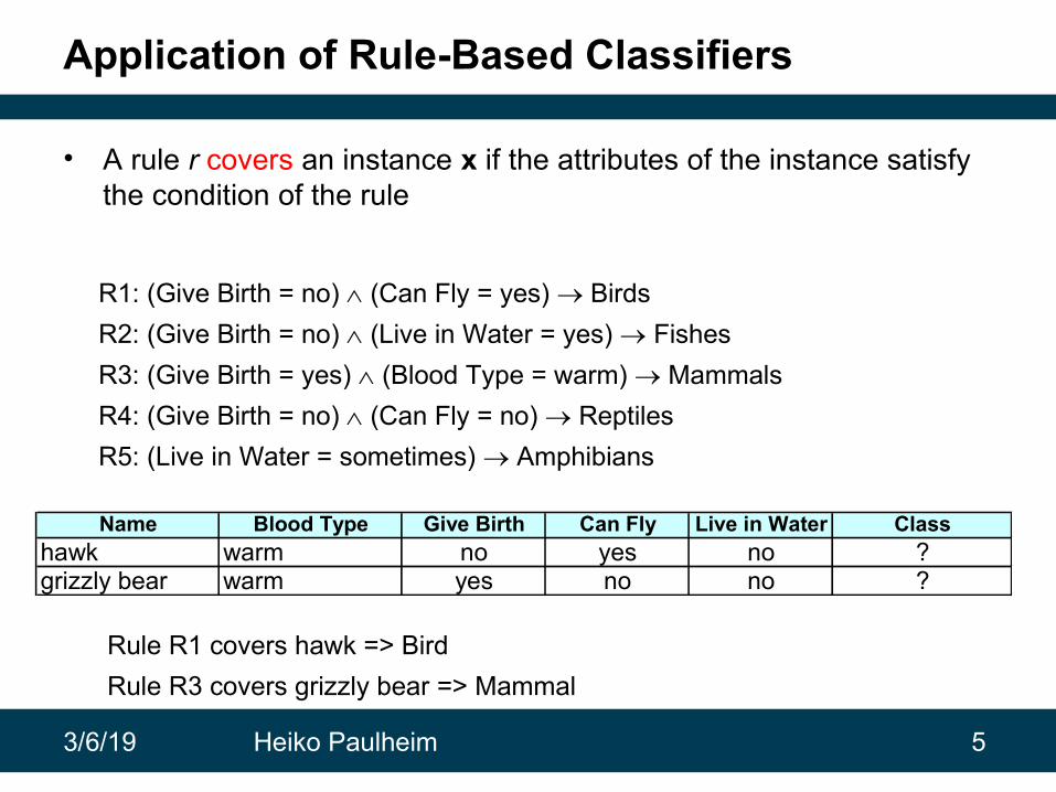
• A rule r covers an instance x if the attributes of the instance satisfy the condition of the rule
R1: (Give Birth = no) (Can Fly = yes) Birds
R2: (Give Birth = no) (Live in Water = yes) Fishes
R3: (Give Birth = yes) (Blood Type = warm) Mammals
R4: (Give Birth = no) (Can Fly = no) Reptiles
R5: (Live in Water = sometimes) Amphibians
Rule R1 covers hawk => Bird
Rule R3 covers grizzly bear => Mammal
Name Blood Type Give Birth Can Fly Live in Water Classhawk warm no yes no ?grizzly bear warm yes no no ?

3/6/19 Heiko Paulheim 6
Rule Coverage and Accuracy
• Coverage of a rule:
– Fraction of records that satisfy the antecedent of a rule
• Accuracy of a rule:
– Fraction of records that satisfy both the antecedent and consequent of a rule
Tid Refund MaritalStatus
TaxableIncome Class
1 Yes Single 125K No
2 No Married 100K No
3 No Single 70K No
4 Yes Married 120K No
5 No Divorced 95K Yes
6 No Married 60K No
7 Yes Divorced 220K No
8 No Single 85K Yes
9 No Married 75K No
(Status=Single) No
Coverage = 40%, Accuracy = 50%

3/6/19 Heiko Paulheim 7
How does a Rule-based Classifier Work?
R1: (Give Birth = no) (Can Fly = yes) Birds
R2: (Give Birth = no) (Live in Water = yes) Fishes
R3: (Give Birth = yes) (Blood Type = warm) Mammals
R4: (Give Birth = no) (Can Fly = no) Reptiles
R5: (Live in Water = sometimes) Amphibians
A lemur triggers rule R3, so it is classified as a mammal
A turtle triggers both R4 and R5
A dogfish shark triggers none of the rules
Name Blood Type Give Birth Can Fly Live in Water Classlemur warm yes no no ?turtle cold no no sometimes ?dogfish shark cold yes no yes ?

3/6/19 Heiko Paulheim 8
Characteristics of Rule-Based Classifiers
• Mutually exclusive rules
– Classifier contains mutually exclusive rules if the rules are independent of each other
– Every example is covered by at most one rule
→ avoids conflicts
• Exhaustive rules
– Classifier has exhaustive coverage if it accounts for every possible combination of attribute values
– Each record is covered by at least one rule
→ enforces each example to be classified
3/6/19 Heiko Paulheim 9
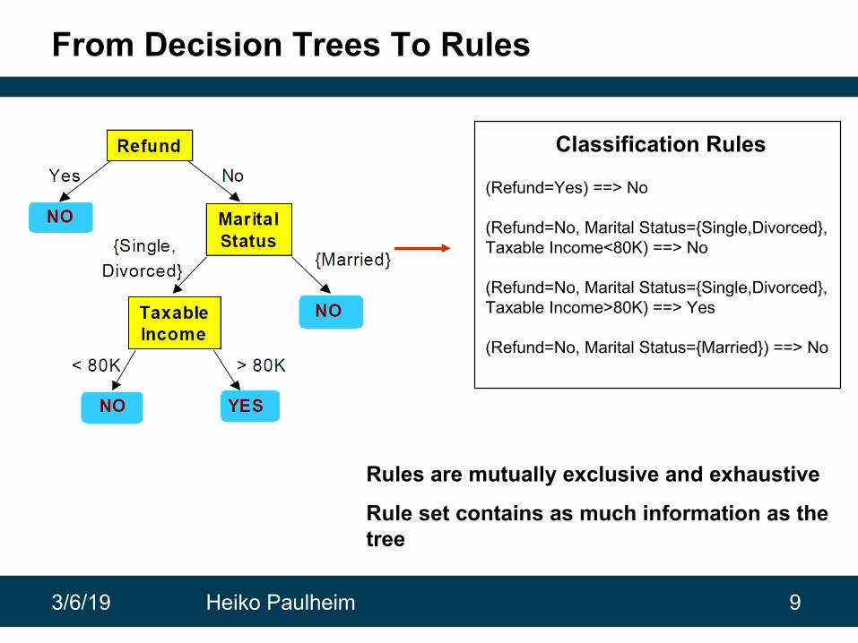
From Decision Trees To Rules
Classification Rules
(Refund=Yes) ==> No
(Refund=No, Marital Status={Single,Divorced},Taxable Income<80K) ==> No
(Refund=No, Marital Status={Single,Divorced},Taxable Income>80K) ==> Yes
(Refund=No, Marital Status={Married}) ==> No
Rules are mutually exclusive and exhaustive
Rule set contains as much information as the tree

3/6/19 Heiko Paulheim 10
Rules Can Be Simplified
Tid Refund MaritalStatus
TaxableIncome Cheat
1 Yes Single 125K No
2 No Married 100K No
3 No Single 70K No
4 Yes Married 120K No
5 No Divorced 95K Yes
6 No Married 60K No
7 Yes Divorced 220K No
8 No Single 85K Yes
9 No Married 75K NoInitial Rule: (Refund=No) (Status=Married) No
Simplified Rule: (Status=Married) No

3/6/19 Heiko Paulheim 11
Possible Effects of Rule Simplification
• Rules are no longer mutually exclusive
– A record may trigger more than one rule
– Solution?
• Ordered rule set
• Unordered rule set – use voting schemes
• Rules are no longer exhaustive
– A record may not trigger any rules
– Solution?
• Use a default class

3/6/19 Heiko Paulheim 12
Ordered Rule Set
• Rules are ranked ordered according to their priority
– An ordered rule set is known as a decision list
• When a test record is presented to the classifier
– It is assigned to the class label of the highest ranked rule it has triggered
– If none of the rules fired, it is assigned to the default class
R1: (Give Birth = no) (Can Fly = yes) Birds
R2: (Give Birth = no) (Live in Water = yes) Fishes
R3: (Give Birth = yes) (Blood Type = warm) Mammals
R4: (Give Birth = no) (Can Fly = no) Reptiles
R5: (Live in Water = sometimes) Amphibians
Name Blood Type Give Birth Can Fly Live in Water Classturtle cold no no sometimes ?

3/6/19 Heiko Paulheim 13
Rule Ordering Schemes
• Rule-based ordering
– Individual rules are ranked based on their quality (e.g., accuracy)
• Class-based ordering
– Rules that belong to the same class appear together
Rule-based Ordering
(Refund=Yes) ==> No
(Refund=No, Marital Status={Single,Divorced},Taxable Income<80K) ==> No
(Refund=No, Marital Status={Single,Divorced},Taxable Income>80K) ==> Yes
(Refund=No, Marital Status={Married}) ==> No
Class-based Ordering
(Refund=Yes) ==> No
(Refund=No, Marital Status={Single,Divorced},Taxable Income<80K) ==> No
(Refund=No, Marital Status={Married}) ==> No
(Refund=No, Marital Status={Single,Divorced},Taxable Income>80K) ==> Yes

3/6/19 Heiko Paulheim 14
Indirect Method: C4.5rules
• Extract rules from an unpruned decision tree
• For each rule, r: A y, – consider an alternative rule r’: A’ y where A’ is obtained by removing
one of the conjuncts in A
– Compare the pessimistic generalization error for r against all r’
– Prune if one of the r’s has a lower pessimistic generalization error
– Repeat until we can no longer improve generalization error

3/6/19 Heiko Paulheim 15
Indirect Method in RapidMiner

3/6/19 Heiko Paulheim 16
Direct vs. Indirect Rule Learning Methods
• Direct Method:
• Extract rules directly from data
• e.g.: RIPPER, CN2, Holte’s 1R
• Indirect Method:
• Extract rules from other classification models (e.g. decision trees, neural networks, etc).
• Example: C4.5rules

3/6/19 Heiko Paulheim 17
Direct methods
• Do not derive rules from another type of model
– but learn the rules directly
• practical algorithms use different approaches
– covering or separate-and-conquer algorithms
– based on heuristic search
The following slides are based on the machine learning course by Johannes Fürnkranz, Technische Universität Darmstadt

3/6/19 Heiko Paulheim 18
A sample task
Temperature Outlook Humidity Windy Play Golf?
hot sunny high false no
hot sunny high true no
hot overcast high false yes
cool rain normal false yes
cool overcast normal true yes
mild sunny high false no
cool sunny normal false yes
mild rain normal false yes
mild sunny normal true yes
mild overcast high true yes
hot overcast normal false yes
mild rain high true no
cool rain normal true no
• Task:
– Find a rule set that correctly predicts the dependent variable from the observed variables

3/6/19 Heiko Paulheim 19
A Simple Solution
IF T=hot AND H=high AND O=overcast AND W=false THEN yes IF T=cool AND H=normal AND O=rain AND W=false THEN yes IF T=cool AND H=normal AND O=overcast AND W=true THEN yes IF T=cool AND H=normal AND O=sunny AND W=false THEN yes IF T=mild AND H=normal AND O=rain AND W=false THEN yes IF T=mild AND H=normal AND O=sunny AND W=true THEN yes IF T=mild AND H=high AND O=overcast AND W=true THEN yes IF T=hot AND H=normal AND O=overcast AND W=false THEN yes IF T=mild AND H=high AND O=rain AND W=false THEN yes
IF T=hot AND H=high AND O=overcast AND W=false THEN yes IF T=cool AND H=normal AND O=rain AND W=false THEN yes IF T=cool AND H=normal AND O=overcast AND W=true THEN yes IF T=cool AND H=normal AND O=sunny AND W=false THEN yes IF T=mild AND H=normal AND O=rain AND W=false THEN yes IF T=mild AND H=normal AND O=sunny AND W=true THEN yes IF T=mild AND H=high AND O=overcast AND W=true THEN yes IF T=hot AND H=normal AND O=overcast AND W=false THEN yes IF T=mild AND H=high AND O=rain AND W=false THEN yes
• The solution is
– a set of rules
– that is complete and consistent on the training examples
• “Overfitting is like memorizing the answers to a testinstead of understanding the principles.” (Bob Horton, 2015)

3/6/19 Heiko Paulheim 20
A Better Solution
IF Outlook = overcast THEN yes
IF Humidity = normal AND Outlook = sunny THEN yes
IF Outlook = rainy AND Windy = false THEN yes
IF Outlook = overcast THEN yes
IF Humidity = normal AND Outlook = sunny THEN yes
IF Outlook = rainy AND Windy = false THEN yes

3/6/19 Heiko Paulheim 21
A Simple Algorithm: Batch-Find
• Abstract algorithm for learning a single rule:
1. Start with an empty theory T and training set E
2. Learn a single (consistent) rule R from E and add it to T
3. return T
• Problem:
– the basic assumption is that the found rules are complete, i.e., they cover all positive examples
– What if they don't?
• Simple solution:
– If we have a rule that covers part of the positive examples,add some more rules that cover the remaining examples

3/6/19 Heiko Paulheim 22
Separate-and-Conquer Rule Learning
• Learn a set of rules, one by one
1. Start with an empty theory T and training set E2. Learn a single (consistent) rule R from E and add it to T 3. If T is satisfactory (complete), return T4. Else:
» Separate: Remove examples explained by R from E» Conquer: goto 2.
• One of the oldest family of learning algorithms– goes back to AQ (Michalski, 60s)
– FRINGE, PRISM and CN2: relation to decision trees (80s)
– popularized in ILP (FOIL and PROGOL, 90s)
– RIPPER brought in good noise-handling
• Different learners differ in how they find a single rule

3/6/19 Heiko Paulheim 23
Separate-and-Conquer Rule Learning

3/6/19 Heiko Paulheim 24
Relaxing Completeness and Consistency
• So far we have always required a learner to learn a complete and consistent theory
– e.g., one rule that covers all positive and no negative examples
• This is not always a good idea (→ overfitting)
• Example: Training set with 200 examples, 100 positive and 100 negative– Theory A consists of 100 complex rules, each covering a single positive
example and no negatives
→ Theory A is complete and consistent on the training set
– Theory B consists of one simple rule, covering 99 positive and 1 negative example
→ Theory B is incomplete and incosistent on the training set
• Which one will generalize better to unseen examples?

3/6/19 Heiko Paulheim 25
Top-Down Hill-Climbing
• Top-Down Strategy: A rule is successively specialized
1. Start with the universal rule R that covers all examples
2. Evaluate all possible ways to add a condition to R
3. Choose the best one (according to some heuristic)
4. If R is satisfactory, return it
5. Else goto 2.
• Almost all greedy s&c rule learning systems use this strategy

3/6/19 Heiko Paulheim 26
Recap: Terminology
predicted + predicted -class + p (true positives) P-p (false negatives) P
class - n (false positives) N-n (true negatives) N
p + n P+N – (p+n) P+N
• training examples• P: total number of positive examples
• N: total number of negative examples
• examples covered by the rule (predicted positive)• true positives p: positive examples covered by the rule
• false positives n: negative examples covered by the rule
• examples not covered the rule (predicted negative)• false negatives P-p: positive examples not covered by the rule
• true negatives N-n: negative examples not covered by the rule

3/6/19 Heiko Paulheim 27
Rule Learning Heuristics
• Adding a rule should
– increase the number of covered negative examples as little as possible (do not decrease consistency)
– increase the number of covered positive examples as much as possible (increase completeness)
• An evaluation heuristic should therefore trade off these two extremes
– Example: Laplace heuristic
• grows with
• grows with
hLap=p+1p+n+2
p→∞n→0

3/6/19 Heiko Paulheim 28
Recap: Overfitting
• Overfitting
– Given
• a fairly general model class
• enough degrees of freedom
– you can always find a model that explains the data
• even if the data contains errors (noise in the data)
• in rule learning: each example is a rule
• Such concepts do not generalize well!
→ Solution: Rule and rule set pruning

3/6/19 Heiko Paulheim 29
Overfitting Avoidance
– learning concepts so that
• not all positive examples have to be covered by the theory
• some negative examples may be covered by the theory

3/6/19 Heiko Paulheim 30
Pre-Pruning
• keep a theory simple while it is learned• decide when to stop adding conditions to a rule
(relax consistency constraint)• decide when to stop adding rules to a theory
(relax completeness constraint)– efficient but not accurate Rule set with three rules
á 3, 2, and 2 conditions
Pre-pruning decisions

3/6/19 Heiko Paulheim 31
Post Pruning

3/6/19 Heiko Paulheim 32
Post-Pruning: Example
IF T=hot AND H=high AND O=sunny AND W=false THEN noIF T=hot AND H=high AND O=sunny AND W=true THEN no IF T=hot AND H=high AND O=overcast AND W=false THEN yes IF T=cool AND H=normal AND O=rain AND W=false THEN yes IF T=cool AND H=normal AND O=overcast AND W=true THEN yes IF T=mild AND H=high AND O=sunny AND W=false THEN no IF T=cool AND H=normal AND O=sunny AND W=false THEN yes IF T=mild AND H=normal AND O=rain AND W=false THEN yes IF T=mild AND H=normal AND O=sunny AND W=true THEN yes IF T=mild AND H=high AND O=overcast AND W=true THEN yes IF T=hot AND H=normal AND O=overcast AND W=false THEN yes IF T=mild AND H=high AND O=rain AND W=true THEN no IF T=cool AND H=normal AND O=rain AND W=true THEN no IF T=mild AND H=high AND O=rain AND W=false THEN yes
IF T=hot AND H=high AND O=sunny AND W=false THEN noIF T=hot AND H=high AND O=sunny AND W=true THEN no IF T=hot AND H=high AND O=overcast AND W=false THEN yes IF T=cool AND H=normal AND O=rain AND W=false THEN yes IF T=cool AND H=normal AND O=overcast AND W=true THEN yes IF T=mild AND H=high AND O=sunny AND W=false THEN no IF T=cool AND H=normal AND O=sunny AND W=false THEN yes IF T=mild AND H=normal AND O=rain AND W=false THEN yes IF T=mild AND H=normal AND O=sunny AND W=true THEN yes IF T=mild AND H=high AND O=overcast AND W=true THEN yes IF T=hot AND H=normal AND O=overcast AND W=false THEN yes IF T=mild AND H=high AND O=rain AND W=true THEN no IF T=cool AND H=normal AND O=rain AND W=true THEN no IF T=mild AND H=high AND O=rain AND W=false THEN yes

3/6/19 Heiko Paulheim 33
IF H=high AND O=sunny THEN no
IF O=rain AND W=true THEN no
ELSE yes
IF H=high AND O=sunny THEN no
IF O=rain AND W=true THEN no
ELSE yes
Post-Pruning: Example

3/6/19 Heiko Paulheim 34
Reduced Error Pruning
• basic idea– optimize the accuracy of a rule set on a separate pruning set
1. split training data into a growing and a pruning set
2. learn a complete and consistent rule set covering all positive examples and no negative examples
3. as long as the error on the pruning set does not increase
delete condition or rule that results in the largest reduction of error on the pruning set
4. return the remaining rules
• REP is accurate but not efficient
– O(n4)

3/6/19 Heiko Paulheim 35
Incremental Reduced Error Pruning
I-REP tries to combine the advantagesof pre- and post-pruning
3/6/19 Heiko Paulheim 36
Incremental Reduced Error Pruning
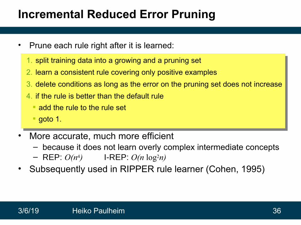
• Prune each rule right after it is learned:
1. split training data into a growing and a pruning set
2. learn a consistent rule covering only positive examples
3. delete conditions as long as the error on the pruning set does not increase
4. if the rule is better than the default rule
add the rule to the rule set
goto 1.
• More accurate, much more efficient– because it does not learn overly complex intermediate concepts– REP: O(n4) I-REP: O(n log2n)
• Subsequently used in RIPPER rule learner (Cohen, 1995)

3/6/19 Heiko Paulheim 37
RIPPER in RapidMiner

3/6/19 Heiko Paulheim 38
Advantages of Rule-Based Classifiers
• As highly expressive as decision trees
• Easy to interpret
• Easy to generate
• Can classify new instances rapidly
• Performance comparable to decision trees

3/6/19 Heiko Paulheim 39
Decision Boundaries: Theory and Practice
• We have seen decision boundaries of rule-based classifiersand decision trees
– both are parallel to the axes
– i.e., both can learn models that are a collection of rectangles
• What does that mean for comparing their performance
– if they learn the same sort of models
– are they equivalent?

3/6/19 Heiko Paulheim 40
Decision Boundaries: Theory and Practice
• Example 1: a checkerboard dataset
– positive and negative points come in four quadrants
– can be perfectly described with rectangles

3/6/19 Heiko Paulheim 41
Decision Boundaries: Theory and Practice
• Example 1: a checkerboard dataset
– positive and negative points come in quadrants
– can be perfectly described with rectangles
• Model learned by a decision tree:
– only the default tree (one node)

3/6/19 Heiko Paulheim 42
Decision Boundaries: Theory and Practice
• What is going on here?
– No possible split improves the purity
– We always have 50% positive and negative examples
– i.e., Gini index is always 0.5
• same holds for other purity measures

3/6/19 Heiko Paulheim 43
Decision Boundaries: Theory and Practice
• Example 1: a checkerboard dataset
– positive and negative points come in quadrants
– can be perfectly described with rectangles
• Model learned by a rule learner:

3/6/19 Heiko Paulheim 44
Decision Boundaries: Theory and Practice
• Example 2:
– a small class inside a large one
– again: can be perfectly described with rectangles

3/6/19 Heiko Paulheim 45
Decision Boundaries: Theory and Practice
• Example 2:
– a small class inside a large one
– again: can be perfectly described with rectangles
• Output of a rule-based classifier:
– no model learned (only a default rule)

3/6/19 Heiko Paulheim 46
Decision Boundaries: Theory and Practice
• What is happening here?
– We try to learn the smallest class
– ...and pre-pruning requires a minimum heuristic
– no initial condition can be selected that exceeds that minimum
best one-condition rule: accuracy=0.17

3/6/19 Heiko Paulheim 47
Decision Boundaries: Theory and Practice
• Example 2:
– a small class inside a large one
– again: can be perfectly described with rectangles
• Decision boundaries of a decision tree classifier:

3/6/19 Heiko Paulheim 48
Decision Boundaries of a k-NN Classifier
• k=1
• Single noise points have influence on model

3/6/19 Heiko Paulheim 49
Decision Boundaries of a k-NN Classifier
• k=3
• Boundaries become smoother
• Influence of noise points is reduced

3/6/19 Heiko Paulheim 50
Decision Boundaries: Theory and Practice
• Decision boundaries are a useful tool
– they show us what model can be expressed by a learner
– e.g., circular shapes are not learned by a decision tree learner
– good for a pre-selection of learners for a problem
• What can be expressed and what is actually learned
– are two different stories
– answer depends heavily on the learning algorithm (and its parameters)
– requires (and provides) more insights into the learning algorithm

Heiko Paulheim
Model Evaluation
● Metrics● how to measure performance?
● Evaluation methods● how to obtain meaningful estimates?

Heiko Paulheim
Model Evaluation
● Models are evaluated by looking at● correctly and incorrectly classified instances
● For a two-class problems, four cases can occur:● true positives: positive class correctly predicted● false positives: positive class incorrectly predicted● true negatives: negative class correctly predicted● false negatives: negative class incorrectly predicted

Heiko Paulheim
Metrics for Performance Evaluation
• Focus on the predictive capability of a model
• Rather than how fast it takes to classify or build models
• Confusion Matrix:
PREDICTED CLASS
ACTUALCLASS
Class=Yes Class=No
Class=Yes TP FN
Class=No FP TN

Heiko Paulheim
Metrics for Performance Evaluation
• Most frequently used metrics:
PREDICTED CLASS
ACTUALCLASS
Class=Yes Class=No
Class=Yes TP FN
Class=No FP TN
FNFPTNTP
TNTP
Accuracy
Accuracy1 RateError

Heiko Paulheim
What is a Good Accuracy?
• i.e., when are you done?
– at 75% accuracy?
– at 90% accuracy?
– at 95% accuracy?
• Depends on difficulty of the problem!
• Baseline: naive guessing
– always predict majority class
• Compare
– Predicting coin tosses with accuracy of 50%
– Predicting dice roll with accuracy of 50%

Heiko Paulheim 56
Limitation of Accuracy: Unbalanced Data
• Sometimes, classes have very unequal frequency
Fraud detection: 98% transactions OK, 2% fraud
eCommerce: 99% don’t buy, 1% buy
Intruder detection: 99.99% of the users are no intruders
Security: >99.99% of Americans are not terrorists
• The class of interest is commonly called the positive class, and the rest negative classes.
• Consider a 2-class problem
Number of Class 0 examples = 9990, Number of Class 1 examples = 10
If model predicts everything to be class 0, accuracy is 9990/10000 = 99.9 %
Accuracy is misleading because model does not detect any class 1 example

Heiko Paulheim
Precision and Recall
Alternative: Use measures from information retrieval which are biased towards the positive class.
Precision p is the number of correctly classified positive examples divided by the total number of examples that are classified as positive.
Recall r is the number of correctly classified positive examples divided by the total number of actual positive examples in the test set.
. .FNTP
TP r
FPTP
TPp

Heiko Paulheim
Precision and Recall Example
• This confusion matrix gives us
precision p = 100% and
recall r = 1%
• because we only classified one positive example correctly and no negative examples wrongly
• We want a measure that combines precision and recall

Heiko Paulheim
F1-Measure
• It is hard to compare two classifiers using two measures
• F1-Score combines precision and recall into one measure
• The harmonic mean of two numbers tends to be closer to the smaller of the two.
• For F1-value to be large, both p and r must be large

Heiko Paulheim
F1-Measure

Heiko Paulheim
Alternative for Unbalanced Data: Cost Matrix
PREDICTED CLASS
ACTUALCLASS
C(i|j) Class=Yes Class=No
Class=Yes C(Yes|Yes) C(No|Yes)
Class=No C(Yes|No) C(No|No)
C(i|j): Cost of misclassifying class j example as class i

Heiko Paulheim
Computing Cost of Classification
Cost Matrix
PREDICTED CLASS
ACTUALCLASS
C(i|j) + -
+ 0 100
- 1 0
Model M1 PREDICTED CLASS
ACTUALCLASS
+ -
+ 162 38
- 160 240
Model M2
PREDICTED CLASS
ACTUALCLASS
+ -
+ 155 45
- 5 395
Accuracy = 67%
Cost = 3798
Accuracy = 92%
Cost = 4350

Heiko Paulheim
ROC Curves
• Some classification algorithms provide confidence scores
– how sure the algorithms is with its prediction
– e.g., Naive Bayes: the probability
– e.g., Decision Trees: the purity of the respective leaf node
• Drawing a ROC Curve
– Sort classifications according to confidence scores
– Evaluate
• correct prediction: draw one step up
• incorrect prediction: draw one step to the right

Heiko Paulheim
ROC Curves
• Drawing ROC Curves in RapidMiner

Heiko Paulheim
Example ROC Curve of Naive Bayes

Heiko Paulheim
Example ROC Curve of Decision Tree Learner

Heiko Paulheim
Interpreting ROC Curves
• Best possible result:
– all correct predictions have higherconfidence than all incorrect ones
• The steeper, the better
– random guessing results in the diagonal
– so a decent algorithm should resultin a curve significantly above the diagonal
• Comparing algorithms:
– Curve A above curve B meansalgorithm A better than algorithm B
• Frequently used criterion
– Area under curve
– normalized to 1

Heiko Paulheim
Methods for Performance Evaluation
• How to obtain a reliable estimate of performance?
• Performance of a model may depend on other factors besides the learning algorithm:
Size of training and test sets (it often expensive to get labeled data)
Class distribution (balanced, skewed)
Cost of misclassification (your goal)
• Methods for estimating the performance
Holdout
Random Subsampling
Cross Validation

Heiko Paulheim
Learning Curve
• Learning curve shows how accuracy changes with varying sample size
• Conclusion: Use as much data as possible for training

Heiko Paulheim
Holdout Method
• The holdout method reserves a certain amount for testing and uses the remainder for training
• Usually: one third for testing, the rest for training
• applied when lots of sample data is available
• For “unbalanced” datasets, samples might not be representative Few or none instances of some classes
• Stratified sample: balances the data Make sure that each class is represented with approximately equal
proportions in both subsets

Heiko Paulheim
Leave One Out
• Iterate over all examples
– train a model on all examples but the current one
– evaluate on the current one
• Yields a very accurate estimate
• Uses as much data for training as possible
– but is computationally infeasible in most cases
• Imagine: a dataset with a million instances
– one minute to train a single model
– Leave one out would take almost two years

Heiko Paulheim
Cross-Validation
• Compromise of Leave One Out and decent runtime
• Cross-validation avoids overlapping test sets
First step: data is split into k subsets of equal size
Second step: each subset in turn is used for testing and the remainder for training
• This is called k-fold cross-validation
• The error estimates are averaged to yield an overall error estimate
• Frequently used value for k : 10– Why ten? Extensive experiments have shown that this is the good choice
to get an accurate estimate
• Often the subsets are stratified before the cross-validation is performed

Heiko Paulheim
Cross-Validation in RapidMiner

3/6/19 Heiko Paulheim 74
Summary
• Rule learning
– another eager method to learn interpretable models
– similar to decision trees
– rectangular decision boundaries
• Evaluation methods
– Accuracy,
– Recall, precision, F1
– ROC Curves
– Cost based evaluation
– Evaluation setups: holdout sets, cross validation

3/6/19 Heiko Paulheim 75
Questions?