Nonlinear Dyn (2007) 49:445–462DOI 10.1007/s11071-006-9108-y

O R I G I N A L A R T I C L E

Data fusion and path-following controllers comparisonfor autonomous vehicles

Urbano Nunes · L. Conde Bento

Received: 15 November 2005 / Accepted: 12 March 2006 / Published online: 18 January 2007C© Springer Science + Business Media B.V. 2007

Abstract This paper presents a comparative study oftwo path-following controllers developed for guidingautonomous vehicles in semi-structured outdoor en-vironments. Part of this paper is focused on the per-formance of two path-following controllers, which areimplemented using two different approaches, the firstusing fuzzy logic and the second using chained sys-tems theory. The control effort and the errors mag-nitude along the path are evaluated in a comparativeway. A magnetic guidance system for autonomous ve-hicles navigation in semi-structured outdoor environ-ments is also described, integrating redundant encodersdata and absolute positioning data provided by on-board magnetic sensors and magnetic markers buried inthe road. Simulation and experimental results are pre-sented showing the effectiveness of the overall controlsystem.

U. Nunes (�)Instituto de Sistemas e Robotica & Dep. Eng.Electrotecnica e de Computadores, Universidade deCoimbra, 3030-290 Coimbra, Portugale-mail: urbano@isr.uc.pt

L. C. BentoInstituto de Sistemas e Robotica & Dep. Eng.Electrotecnica, Instituto Politecnico de Leiria 2411-901Leiria, Portugale-mail: conde@isr.uc.pt

Keywords Data fusion . Path-following . Intelligentvehicles . Fuzzy logic controller . Chained formsystems . Magnetic guidance

1 Introduction

A new approach for mobility providing an alternativeto the private passenger car, by offering the same flexi-bility but with much less nuisances, is emerging, basedon fully automated electric vehicles, named cybercars[6, 18]. A fleet of such vehicles might be an importantelement in a novel individual, door-to-door, transporta-tion system to the city of tomorrow. These vehicles mustbe user-friendly, easy to handle and functioning withtotal safety, not only for passengers but also for otherroad users. These vehicles are already in operation inspecific environments featuring short trips at low speed[3, 6].

For fully automated operation, path-following andlateral controllers have been widely investigated, usingdifferent control strategies, such as fuzzy-logic, slid-ing mode and chained form based controllers. In [22],a simplified nonlinear kinematics model is proposed,intended to ease the design and implementation of a sta-ble lateral controller. Fuzzy-logic controllers (FLC) aredescribed in [10, 11]. The design and simulation eval-uation of trajectory-tracking and path-following con-trollers based on sliding mode control is described in[21].

Springer

446 Nonlinear Dyn (2007) 49:445–462

Ve

loci

ty P

lan

ne

r

ErrorCalculation

Vehicle&

encodersChained Form Module

Fuzzy Logic Module

Controller typeMulti Target

Detection and Tracking System

Laserscanner Path Following Controller

Magnetic Sensors

Vehicle’s Pose

Estimator

Lateral Controller

EKF odometry

ExternalFactors

PathGenerator

sw

c

c

ϕυϕ

Range-bearingData

Fig. 1 Navigation systemarchitecture. Two lateralcontrollers were developed.Although only one runs foreach set of experiments theyare both represented in thefigure as fuzzy logic moduleand chained form module

This paper describes developments of an au-tonomous navigation system applied on guiding afour-wheel actuated electrical vehicle moving in semi-structured outdoor environments. Its purpose is to pro-vide guidance control with anti-collision behaviour forlow-speed vehicles moving in cybercars scenarios. Cy-bercars [6] have to satisfy challenging requirementslike following a path, with high accuracy, in narrowspaces shared with other vehicles and in some areaswith pedestrians, providing ride comfort, with low levelof jerk and assuring complete safety with human driver-less control. A suitable controller has to be chosen ful-filling the previous requirements, which motivated thecomparative study of the two lateral control strategiespresented in this paper.

Odometry being essential for autonomous naviga-tion is not enough due to its relative and integrativenature. So, it is required to complement odometric datawith absolute positioning. Data fusion of ABS sensorsand GPS for outdoor localization, based on an ExtendedKalman Filter (EKF) had been presented in [4]. Self-localization, given a map of the environment, and themore challenging problem of simultaneous localizationand mapping are two examples of key mobile robotproblems requiring positioning data. The most com-monly used localization probabilistic approaches em-ploy Kalman filtering (e.g. [13]), grid-based Markovlocalization [9] and Monte Carlo methods [8]. Onthe other hand, the California Partners for AdvancedTransit and Highways (PATH) Program has beengiven important contributions in the development of a

reference system based on magnets for vehicle lateralguidance/control [24, 27].

1.1 Navigation architecture

The overall navigation system (see Fig. 1) is composedof three main subsystems, which are designated bypath-following controller (PFC), vehicle’s pose esti-mator (VPE) and multi-target detection and trackingsystem (MTDTS). The MTDTS is described in [16],while the PFC and VPE modules are addressed in thispaper. The PFC is made up of two main modules: thevelocity planner (VP) and the lateral controller (LC).The VP provides local target points of the referencetrajectory and computes the maximum and the com-fortable velocities, taking into account external factors.The considered external factors are tyre characteristicsand passenger comfortable lateral and longitudinal ac-celerations.

Two lateral controllers, one fuzzy-logic-based andanother using chained form theory, were developedwhich are described and compared in this paper.

2 Kinematics and odometry model

2.1 Kinematics model

A Robucar (manufactured by Robosoft) is used inthe autonomous navigation experiments. It is equippedwith four wheels, each one driven by an independent

Springer

Nonlinear Dyn (2007) 49:445–462 447

o

La

dcp

e

CP

xPi-1

Pi

Pi+1

d

e

x

yw

CGR

dtg

e

dra

e

θ

θθ

Σ

Σ

ϕ

Fig. 2 Illustrative construction of lateral and heading errors (inreal situation the discrete path points Pi are much closer betweeneach other, when compared with the vehicle dimensions). Pi de-note the points that define the reference trajectory; dcp

e and d rae

are the lateral errors at CP and rear axle, respectively; d tge is the

perpendicular distance between the rear axle midpoint and the

current tangent to the path; θ , θ cpe and θd are the orientation of the

vehicle, heading error and desired heading, respectively. W � andR� represent respectively the world coordinate system and thevehicle local coordinate system with its origin at the midpoint ofthe rear axle and its x-axis aligned with the longitudinal axis ofthe vehicle

motor equipped with its own encoder. The vehicle hasthe ability to steer both the rear and the front pair ofwheels [19], but in our models and experiments onlyfront steering has been used due to uncertainties onthe odometry model of a double steered vehicle. Theclassical model considers an imaginary wheel at themidpoint of the wheels axles, so that it is oriented inthe direction of the steering command.

The configuration of the vehicle can be describedwithout ambiguity by (x, y, θ ) (see Fig. 2):

– x and y are the coordinates of the rear axle centrewith respect to the W � coordinates;

– θ is the vehicle heading with respect to the W �

coordinates.

The vehicle kinematic equations are derived ac-cording to pure rolling, non-slipping and rigid bodyassumptions. Therefore, a linear velocity vector andinstantaneous rotation centre exists at the referenceframe located at the midpoint of the rear axle R� andthe velocity is directed along the vehicle axle. Kinemat-ics models have the property of keeping the steering and

velocity of the vehicle completely decoupled, thereforeturning easy the kinematics-based control design. Thekinematic model of the vehicle, for a reference framelocated at the midpoint of the rear axle R�, is

⎡⎢⎢⎢⎣x

y

θ

ϕ

⎤⎥⎥⎥⎦ =

⎡⎢⎢⎢⎣cos(θ )

sin(θ )tan ϕ

L

0

⎤⎥⎥⎥⎦ v1 +

⎡⎢⎢⎢⎣0

0

0

1

⎤⎥⎥⎥⎦ v2 (1)

where v1 represents the linear velocity of the vehicle,v2 is the steering angular velocity, L is the distancebetween the rear and front axles, ϕ is the front steer-ing angle and θ is the vehicle orientation in the worldcoordinate system, as depicted in Fig. 2.

A different point of view and more useful in terms ofpath-following is the one that describes the vehicle be-haviour in terms of the path coordinates [14]. Assumingthat the vehicle has to follow a path defined by its arclength, one can define the following error variables:

Springer

448 Nonlinear Dyn (2007) 49:445–462

� d tge the perpendicular distance between the rear axle

midpoint and the current tangent to the path.� θtge the angle between the current tangent to the path

and the x-axis of the vehicle.

Under these assumptions, one can derive the kine-matic model in terms of the path coordinates,

⎡⎢⎢⎢⎢⎣s

d tge

θtge

ϕ

⎤⎥⎥⎥⎥⎦ =

⎡⎢⎢⎢⎢⎢⎢⎢⎣

cos(θ tge )

1−d tge c(s)

sin(θ tge )

tan ϕ

L − c(s) cos(θ tge )

1−d tge c(s)

0

⎤⎥⎥⎥⎥⎥⎥⎥⎦v1 +

⎡⎢⎢⎢⎣0

0

0

1

⎤⎥⎥⎥⎦ v2 (2)

where c(s) is the curvature of the path.

2.2 Odometry model

Let the vehicle position be represented by the middlepoint rear axle M with Cartesian coordinates (xk, yk)at time tk , as shown in Fig. 3. The vehicle local co-ordinate system is defined as having origin M and itsx-axis aligned with the longitudinal axis of the car. θk

is the vehicle heading angle at time tk . Assuming thatthe vehicle’s motion is locally circular, its position and

Fig. 3 Vehicle geometrical configuration

Table 1 Vehicle geometrical configuration parameters

L Car length (distance between rear and front axle)e Half-track (half car width)ϕR Steering angle from right wheelϕL Steering angle from left wheelϕ Steering angle of the virtual front wheelD Curvature radius of virtual front wheelρ Curvature radius of the rear axle center

orientation at time tk is given by⎧⎪⎨⎪⎩xk+1 = xk + � cos(θk + ω/2)

yk+1 = yk + � sin(θk + ω/2)

θk+1 = θk + ω

(3)

where � is the arc length and ω the elementary rotation.Assuming that there is no wheel slippage and using onlydata from the rear wheels encoders, then

� = �RR + �RL

2, ω = �RR − �RL

2e(4)

where e is the half distance between wheels and �RR

and �RL are calculated using the right and left wheelencoders measurements, respectively.

The vehicle geometrical configuration parametersare illustrated in Fig. 3 and are summarized inTable 1.

3 Path-following controllers

The vehicle can execute a point-to-point stabilization,path-following and trajectory tracking. Point-to-pointstabilization requires that the vehicle moves from pointA to point B with no restrictions on its movement be-tween these two points. While in path-following, thevehicle must move along a geometric path, in trajec-tory tracking, the vehicle must move along a geometricpath at a given speed.

This paper addresses the path-following problem.The PFC is made up of two main modules: VP andLC. Two LCs are described in this section with thefollowing set of inputs:

– for the chained-form-based controller:

uCF = [θ tg

e , d tge , c(s)

](5)

Springer

Nonlinear Dyn (2007) 49:445–462 449

– for the fuzzy controller:

uFL = [θ cpe , dcp

e , �θ cpe , �dcp

e , timp, dile, c(s), v]

(6)

where v denotes the linear reference velocity, timp is thetime-to-collision computed in the MTDTS, dile is theinline lateral error (see Section 3.2.2) and the differen-tial errors �dcp

e and �θcpe , at the control point (CP) are

given by

�dcpe = dcp

e (k) − dcpe (k − 1) (7)

and

�θ cpe = θ cp

e (k) − θ cpe (k − 1) (8)

Collision avoidance is achieved by controlling the ve-hicle’s reference velocity, reducing or even stoppingthe vehicle in situations of eminent danger. The maingoal of the path-following controller is to ensure thatthe vehicle follows the predefined reference path withappropriate orientation. For the fuzzy logic controllerthis can be understood as a task of minimizing the ve-hicle lateral and heading errors (dcp

e , θcpe ) with respect

to the reference path, at a given control point (CP) lo-cated at a distance La denoted by lookahead distance,as illustrated in Fig. 2.

For both controllers the curvature along the path c(s)is estimated as described in [15]. From the third row of(2) one can obtain a linearly parameterizable system inc(s) written by

y = wa (9)

where

y = v1d tge tan ϕ

L− θ tg

e (10)

w = v1 cos(θ tge ) + v1d tg

e tan ϕ

L− θ tg

e d tge (11)

a = c(s) (12)

Knowing w and y, an estimate of a, i.e. a, is obtainedusing the least squares estimator:

J =∫ t

0(y − wa)2 dτ (13)

Solving for a so as to minimize J , the following updateequation for a is obtained:

˙a = P(wy − w2a) (14)

where P and its update equation P are given by:

P = 1∫ t0 w2dτ

(15)

P = −P2w2 (16)

Each controller has to provide the same control vec-tor ([ϕc, vc, ϕsw]) to the traction control level, whereϕc (in degrees) is the steering angle, vc (m s−1) is thevelocity command and ϕsw is the rear steering switchthat controls the two possible driving modes: dual andpark modes. In dual mode the rear axle steers in op-posite direction of the front axle, while in park modethe rear and front axle steers in the same direction. Thechained form controller provides a steering angle ve-locity command (ϕc) which has to be integrated beforebeing issued to the traction control level (see Fig. 4).

The traction controller is common for any controllertype, thus providing modularity to the system architec-ture. For each wheel and steering axle there is an in-dependent PID controller as shown in Fig. 4, enablingcontrol of wheel slippage and the two possible drivingmodes: front steered and double steered. Although itis possible to use the double steered option, only frontsteering was used in the implemented controllers.

3.1 Velocity planner

The VP module calculates the linear reference veloc-ity, as well as determines the local reference trajectorypoints. One main objective taken into account was tomake the trip as comfortable as possible, i.e. to give thesystem the capability of fully controlling the smooth-ness of the acceleration profile either lateral or longi-tudinal.

A Canadian study [7] used a highway testing groundto test speed and lateral acceleration on both wet anddry pavement on horizontal curves. They found that“comfortable lateral acceleration” and “speed environ-ment” limited the driver’s speed, while pavement sur-face conditions (dry or wet) and the driver’s gender did

Springer

450 Nonlinear Dyn (2007) 49:445–462

PIDFRONT RIGHTWHEEL

PIDREAR LEFT

WHEEL

ROBUCAR

MOTORFR

MOTORRL

ENCFR

ENCRL

ODOMETRY

PIDFRONT

STEERING

PIDREAR

STEERING

ROBUCAR

MOTORFST

MOTORRST

ENCFST

ENCRST

-

+

-+

-+

-

+

FRw′

RLw′

FSTw′

RSTw′

FRw

RLw

FSTw

RSTw

INVERSEKINEMATICS

sw

c

c

ϕυϕ

ODOMETRYk

k

k

y

x

+

+

+

1

1

1

θ

Vehicle’s Pose Estimator

ErrorCalculation

Velocity Planner

Multi Target Detection and

Tracking System

Traction Control Level

FUZZY LOGIC CONTROLLER

CHAINEDFORM

CONTROLLER

ΔΔ

υ

θ

θ

)(sc

d

t

d

d

ILE

imp

cpe

e

cpe

e

)(sc

d tpe

eθ ∫ )(tf

Path Following Control Level

= 0sw

c

ϕυ

[ ]cϕ.

Fig. 4 Lateral and tractioncontrol structures

not. Drivers adjusted their comfortable speed accord-ing to their comfortable lateral acceleration tolerance,approximately between 3.43 and 3.92 m s−2. Anotherstudy [26] revealed the comfortable longitudinal ac-celeration, i.e. steady deceleration under expected-stopconditions; drivers generally exert an average steadybraking force of −3.43 m s−2. This amount of brakingforce seems comfortable for most drivers.

The previous acceleration limits were used to setup the maximum comfort acceleration amc and maxi-mum comfort velocity vmc. The maximum accelerationwithout slipping amws and maximum velocity withoutslipping vmws still had to be computed to cope with un-expected situations. To estimate vmws, it is necessary

to know the forces that actuate on the vehicle, whichare basically the horizontal forces, the wheel groundcontact forces, the force that the vehicle exerts on theground and the wind force over the vehicle (air resis-tance). In this study we consider a plane road and nowind force effects are taken into account.

The friction force is proportional to the normal re-action, where the proportionality factor is the frictioncoefficient μ (static or dynamic).

Taking into account the previous assumptions onecan derive the maximum velocity without slipping

vmws =√

rg(μ cos(ψ) + sin(ψ)) (17)

Springer

Nonlinear Dyn (2007) 49:445–462 451

Fig. 5 Vehicle following a given path. In the figure some sam-pling points are marked (11, 21, 31 and 41 ) (x-axis and y-axisare in meters)

where g is the gravity acceleration, r the curvature ra-dius and ψ denotes the roll angle of the vehicle.

An estimate of μ is obtained by the following equa-tion:

μ(S) = (c1(1 − e−c2 S) − c3S)e−c4 Sv(1 − c5 F2

z

)(18)

where S is the resultant slip and the constants ci

(i = 1 . . . 5) are characteristic parameters of varioustypes of road [12]. The velocity vmc determines theintended vehicle velocity used in the vehicle motion.The vmws has a more ruggedness profile, as can be ob-served in Fig. 6, which shows the velocity profilescorresponding to the example of a vehicle followingthe path depicted in Fig. 5. In order to fulfil the amws,or the amc constraints, the vehicle should start brakingin advance being more restrictive for the amc profile(see Fig. 7). The profit of being more restrictive is asmoother variation on the amc profile.

3.2 Fuzzy logic lateral controller

The fuzzy LC is composed of four independent mod-ules: front steering controller, rear steering switch,velocity command generator and lookahead distancecomputation (see Fig. 8). In order to properly avoidcollisions with obstacles the time-to-impact timp (alsoreferred here as time-to-collision), provided by theMTDTS, is integrated in the velocity command gener-ator. All modules are fuzzy logic based. Figure 8 showsthe LC identifying the fuzzy logic inference flow fromthe input variables to the output variables.

The fuzzy controller is characterized in Table 2. Thefuzzification transforms numerical variables into fuzzysets, which can be manipulated by the controller. Thecontroller uses fuzzy triangular membership functionsand trapezoidal membership functions to encode inputsand outputs. The controller uses min and max connec-tives and a singleton sum–product inference mecha-nism. The center of gravity defuzzification method wasused. Because more than one output term can be eval-uated as valid, the defuzzification method must be acompromise between different results. The center ofgravity method was chosen because it takes into ac-count, better than any other method, the distribution ofthe resultant fuzzy set. In this method, the defuzzifiedvalue u is a weighted sum of the term membership:

u =∑

i μ(xi )xi∑i μ(xi )

(19)

where xi is the degree of activation of the i th rule andμ(xi ) is the output membership function.

The input sets, the output sets, part of the fuzzyknowledge base and some of the membership functions

5 01 51 02 52 03 53 04

0

5

01

51 stniartsnoc tuohtiw v

v swmv cm

[ms

]

[sampling points]

-1

Fig. 6 Velocity profiles forthe example of Fig. 5(x-axis denotes thesampling points and y-axisis in m s−1)

Springer

452 Nonlinear Dyn (2007) 49:445–462

5 01 51 02 52 03 53 04

51-

01-

5-

0

5

01

51

02

a stniartsnoc tuohtiw

a swma cm

[ms

]-2

[sampling points]

Fig. 7 Acceleration profiles for the example of Fig. 5 (x-axisdenotes the sampling points and y-axis is in m s−2)

Fig. 8 Fuzzy lateral controller modules

are presented in [2]. The knowledge base of the LCexpresses how the system should react, a complete de-scription can be found in [1].

3.2.1 Front steering module

The front steering module computes the steering com-mand ϕc. The purpose is to minimize both the orien-tation error θ

cpe and the lateral error dcp

e . A steeringincrement fuzzy variable (ϕinc) is computed in order toachieve a faster recovery from an undesirable pose. ϕinc

is the output of a fuzzy module which has as inputs c(s)and �θ

cpe .

Table 2 Fuzzy controller structure

Fuzzy system Structure

Input variables 8Output variables 4Intermediate variables 1Rule blocks 5Rules 615Membership functions 48

3.2.2 Rear steering switch module

The rear steering switch module enables dual mode orpark mode. The inputs of this module are �dcp

e and theinline lateral error dile given by

dile =∣∣∣∣dcp

e

dcge

∣∣∣∣ + |θ cpe | (20)

If �dcpe is decreasing and dile is small, this module

steers the rear wheels in the same direction as the frontwheels; the result is a decrease in the vehicle’s yawmotion. The yaw motion is necessary for executing amanoeuvre but is not desired from the point of viewof the vehicle’s stability control [20]. This module wasonly implemented and tested in simulations.

3.2.3 Velocity command generator module

The inputs of this module are �dcpe , dcp

e , �θcpe , θ cp

e andthe timp. This module computes a weight factor assign-ing a level of significance to the reference velocity,i.e. if the errors have a high magnitude or the time-to-collision has a low magnitude then the velocity must bedecreased, otherwise the reference velocity is applied.This module is of extreme importance since collisionavoidance is decided here, i.e. if the timp is small, thenthe vehicle velocity is reduced or the vehicle is evenstopped.

3.2.4 Lookahead distance computation module

This module computes the lookahead distance, La ,which is a function of the vehicle velocity, v. If thevelocity increases, the damping factor of the closedloop system gets worse and is improved by increasingthe lookahead distance. The lookahead distance pro-vides a prediction behaviour to the controller, since it

Springer

Nonlinear Dyn (2007) 49:445–462 453

enables the control point to be far ahead of the CG ofthe vehicle, see Fig. 2.

3.3 Chained-form-based lateral controller

The control law designed here, based upon the kine-matics model, uses the chained systems theory [5]. Al-though mobile robot models cannot be linearized, it hasbeen proven that one can convert the nonlinear systemin an almost linear system, termed as chained form. A2-input and n-state chain form system (2, n) has thefollowing structure:

x1 = u1

x2 = u2

x3 = x2u1 (21)

...

xn = xn−1u1

The vehicle model from Equation (2) can be con-verted into chained form using the following changeof coordinates and input transformations [14], respec-tively:

x1 = s

x2 = − c′(s)d tge tan

(θ tg

e

)− c(s)(1 − d tg

e c(s))1 + sin2

(θ

tge

)cos2

(θ

tge

)+ (1 − d tg

e c(s))2 tan(ϕ))

L cos3(θ

tge

)x3 = (1 − d tg

e c(s)) tan(θ tge )

x4 = d tge (22)

v1 = 1 − d tge c(s)

cos(θ

tge

) u1

v2 = α2(u2 − α1u1) (23)

where c′(s) denotes the derivative of c with respect tos, and

α1 = ∂x2

∂s+ ∂x2

∂d tge

(1 − d tg

e c(s))

tan(θ tg

e

)

+ ∂x2

∂θtge

(tan(ϕ)

(1 − d tg

e c(s))

L cos(θ tge )

− c(s)

)

α2 = l cos3(θ tge ) cos2(ϕ)(

1 − d tge c(s)

)2 (24)

and the other variables are defined in Fig. 2.Although the system has two inputs, u1 and u2, this

model can be considered single input if u1 is knowna priori. Then the objective of the control law is toachieve path-following under the assumption that thevehicle linear velocity u1 is constant.

The controller was made using the smooth time-varying feedback stabilization method described in[14], where control is either smooth or at least con-tinuous with respect to the robot state.

As a first step, the variables of the chained form areredefined

χ = (χ1, χ2, χ3, χ4) = (x1, x4, x3, x2) (25)

resulting in the chained form system

χ1 = u1

χ2 = χ3u1 (26)

χ3 = χ4u1

χ4 = u2

The above reordering is simply an exchange betweenthe second and fourth coordinates. Path-following isachieved via input scaling, which requires zeroing theχ2, χ3 and χ4 variables, independently from χ1. Thesystem (26) is controllable if u1 is a piecewise contin-uous, bounded and strictly positive (or negative) func-tion, as stated in [14]. Therefore, u2 is the only inputto the system as long has u1 is known a priori:

u2(χ2, χ3, χ4, t) = −k1|u1(t)|χ2

− k2u1(t)χ3 − k3|u1(t)|χ4 (27)

The complete deducing of the controller and itsbackground theory are described in [14].

Springer

454 Nonlinear Dyn (2007) 49:445–462

4 Vehicle pose estimator

4.1 EKF odometry

The odometry model in (3) and (4) is based only onthe rear wheels encoder. Using also the front wheelsencoders, redundant data become available, which canbe used to produce better estimates of � and ω. Thesteering angle of left and right wheels can be expressedby

ϕL = arctan

(tan(ϕ)L

L − e tan(ϕ)

)(28)

ϕR = arctan

(tan(ϕ)L

L + e tan(ϕ)

)(29)

where ϕ is the steering angle of the virtual frontwheel.

From (28) and (29) and knowing that � = ρω, aset of equations can be established which relates theencoders measurements (from each of the four wheelsand steering) with the parameters � and ω [4]:⎧⎪⎪⎪⎪⎪⎪⎨⎪⎪⎪⎪⎪⎪⎩

tan(ϕ) = L ω�

�RL = � − eω

�RR = � + eω

�FL cos(ϕL) = � − eω

�FR cos(ϕR) = � + eω

(30)

Therefore, considering x = [�, ω]T and

y = [tan(ϕ), �RL, �RR, �FL cos(ϕL), �FR cos(ϕR)]T

the state and measurement vectors, respectively, anEKF can be applied as in [4] to estimate the state vector,from the redundant data.

4.2 Odometry confidence tests and simulation

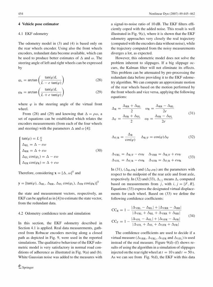
In this section, the EKF odometry described inSection 4.1 is applied. Real data measurements, gath-ered from Robucar encoders moving along a closedpath as depicted in Fig. 9, were used in the reportedsimulations. The qualitative behaviour of the EKF odo-metric model is very satisfactory in normal road con-ditions of adherence as illustrated in Fig. 9(a) and (b).White Gaussian noise was added to the measures with

a signal-to-noise ratio of 10 dB. The EKF filters effi-ciently coped with the added noise. This result is wellillustrated in Fig. 9(c), where it is shown that the EKFodometry approaches very closely the real trajectory(computed with the encoders data without noise), whilethe trajectory computed from the noisy measurementsdiverges a lot, as expected.

However, this odometric model does not solve theproblem inherent to slippages. If a big slippage oc-curs, the Kalman filter will not eliminate its effects.This problem can be attenuated by pre-processing theredundant data before providing it to the EKF odome-try algorithm. We can compute an approximate motionof the rear wheels based on the motion performed bythe front wheels and vice versa, applying the followingequations:

�R = �RR + �RL

2ωR = �RR − �RL

2e

�F = �FR + �FL

2ωF = �FR − �FL

2e

(31)

�F/R = �R

cos(ϕ)�R/F = cos(ϕ)�F (32)

�VRL = �R/F − eωF �VRR = �R/F + eωF

�VFL = �F/R − eωR �VFR = �F/R + eωR(33)

In (31), (�R,ωR) and (�F,ωF) are the parameters withrespect to the midpoint of the rear axle and front axle,respectively. In (32) and (33), �i/j means �i computedbased on measurements from j , with i, j = {F, R}.Equations (33) express the designated virtual displace-ments for each wheel. Based on (33) we define thefollowing confidence coefficients:

CCR = 1 − |�VRL − �RL| + |�VRR − �RR||�VRL + �RL + �VRR + �RR|

CCF = 1 − |�VFL − �FL| + |�VFR − �FR||�VFL + �FL + �VFR + �FR|

(34)

The confidence coefficients are used to decide if avirtual measure (�VRR, �VRL, �VFR and �VFL) is usedinstead of the real measure. Figure 9(d)–(f) shows re-sults of using the algorithm in a simulation of slippagesinjected on the rear right wheel at t = 10 s and t = 50 s.As we can see from Fig. 9(d), the EKF with this data

Springer

Nonlinear Dyn (2007) 49:445–462 455

NoiseRealKalman

20

15

10

5

0

-5

-10

0 10 20 30 40 50 60 70

t[ ]s

[]

mm

NoiseRealKalman

0 10 20 30 40 50 60 70

t[ ]s

0.015

0.01

0.005

[]

-0.005

-o.01

-0.015

rad 0

RealKalmanNoise

492 494 496 498 500 502 504 506 508 510 512x[ ]m

518

516

514

512

y[]

508

506

504

502

m 510

(c)(b)(a)

0 10 20 30 40 50 60-5

0

5

10

15

20

25

30

35

40

t[ ]s

[]

mm

NoiseEKF-CT

495 500 505 510 515

502

504

506

508

510

512

514

516

518

520

x[ ]m

y[

]m

EKF-CTCTReal

485 490 495 500 505 510

500

505

510

515

520

x[ ]m

y[

]m

EKFReal

(f)(e)(d)

Fig. 9 (a) EKF estimation for � (real – encoders measures; noise– measures with white noise; Kalman – obtained estimation);(b) EKF estimation for ω (real – encoders measures; noise –measures with white noise; Kalman – obtained estimation); (c)Odometry results with and without the EKF (real – encodersmeasures; noise – measures with white noise; Kalman – ob-tained estimation); (d) � estimation with a simulated slippage(noise – encoders measures with a simulated slippage at t = 10

and t = 50 s; EKF-CT – estimation with EKF-CT); (e) Odome-try obtained with CT (CT – path estimated applying the CT andodometry model (3); real – path without the simulated slippage;EKF-CT – path estimated applying the EKF-CT); (f) Odome-try obtained with EKF without using CT (real – path withoutthe simulated slippage; EKF – path estimated applying the EKFodometry)

pre-processing, henceforth known as EKF-CT odome-try (EKF odometry with confidence tests), will not fol-low the slippage, hence the algorithm detected a wrongmeasure and replaced it by the virtual measure, com-puted based on the other measures. Estimated paths us-ing the EKF-CT and the EKF algorithms are illustratedin Fig. 9(e) and (f). In both, the solid line represents thereal path. In Fig. 9(e), the dotted line represents the es-timated path using odometry model (3) and confidencetests.

4.3 Fusion of odometry and positioning absolute data

The vehicle is equipped with sensors which provideabsolute positioning data: (1) a SICK laser which pro-vides range-bearing data (d, φ) associated to visiblelandmarks; (2) two magnetic sensing rulers, one placedon the front and the other on the rear of the vehicle.The magnetic sensing rulers developed at ISR [17],based on an array of adjacent Hall effect sensors, de-

tect robustly magnetic markers which are placed on theground defining centerpoints of the path to be followedby the vehicle.

The fusion of odometry data with absolute position-ing data is made by means of EKFs. The vehicle’spose is defined by the Cartesian coordinates (x, y) andheading (θ ), which are the state variables of the EKF.The state variables of the EKF odometry (Section 4.1)are here treated as inputs to the EKF data fusion, i.euk = (�, ω) with an associated noise covariance ma-trix �k . The range-bearing measurements associatedto each landmark are treated as measurements in thefusion process.

(1) System model: The system model is defined bythe kinematic nonlinear equations (3), with statevector xk = [xk yk θk]T, and input uk = [�k ωk]T,which can be written in the compact form (includ-ing noises):

xk = f(xk−1, uk−1, γk−1, σk−1) (35)

Springer

456 Nonlinear Dyn (2007) 49:445–462

M

X

Y

yk

xk

magneticruler

magnet

d

dl

xlaser

ylaser

x

y

laser

scanner

magneticruler

landmark

m

a

θ

α

φ

Κ

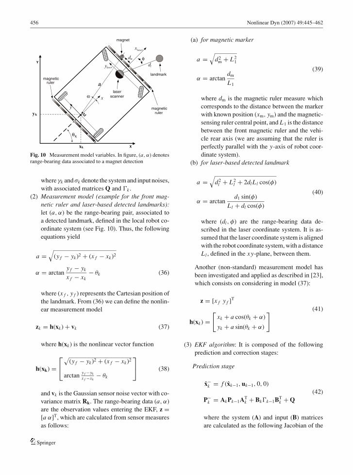
Fig. 10 Measurement model variables. In figure, (a, α) denotesrange-bearing data associated to a magnet detection

where γk and σk denote the system and input noises,with associated matrices Q and �k .

(2) Measurement model (example for the front mag-netic ruler and laser-based detected landmarks):let (a, α) be the range-bearing pair, associated toa detected landmark, defined in the local robot co-ordinate system (see Fig. 10). Thus, the followingequations yield

a =√

(y f − yk)2 + (x f − xk)2

α = arctany f − yk

x f − xk− θk (36)

where (x f , y f ) represents the Cartesian position ofthe landmark. From (36) we can define the nonlin-ear measurement model

zk = h(xk) + vk (37)

where h(xk) is the nonlinear vector function

h(xk) =⎡⎣√

(y f − yk)2 + (x f − xk)2

arctan y f −yk

x f −xk− θk

⎤⎦ (38)

and vk is the Gaussian sensor noise vector with co-variance matrix Rk. The range-bearing data (a, α)are the observation values entering the EKF, z =[a α]T, which are calculated from sensor measuresas follows:

(a) for magnetic marker

a =√

d2m + L2

1

α = arctandm

L1

(39)

where dm is the magnetic ruler measure whichcorresponds to the distance between the markerwith known position (xm, ym) and the magnetic-sensing ruler central point, and L1 is the distancebetween the front magnetic ruler and the vehi-cle rear axis (we are assuming that the ruler isperfectly parallel with the y-axis of robot coor-dinate system).

(b) for laser-based detected landmark

a =√

d2l + L2

l + 2dl Ll cos(φ)

α = arctand1 sin(φ)

Ll + dl cos(φ)

(40)

where (dl , φ) are the range-bearing data de-scribed in the laser coordinate system. It is as-sumed that the laser coordinate system is alignedwith the robot coordinate system, with a distanceLl , defined in the xy-plane, between them.

Another (non-standard) measurement model hasbeen investigated and applied as described in [23],which consists on considering in model (37):

z = [x f y f ]T

(41)

h(xk) =[

xk + a cos(θk + α)

yk + a sin(θk + α)

]

(3) EKF algorithm: It is composed of the followingprediction and correction stages:

Prediction stage

x−k = f (xk−1, uk−1, 0, 0)

(42)P−

k = AkPk−1ATk + Bk�k−1BT

k + Q

where the system (A) and input (B) matricesare calculated as the following Jacobian of the

Springer

Nonlinear Dyn (2007) 49:445–462 457

0 100 200 300 400 500 600 700-4

-2

0

2

4

6

8

10

12

14

[sampling points]

[degre

es]

Theta error (FUZZY)

Theta error (CF)

6 6.2 6.4 6.6 6.8 7 7.2 7.4 7.6 7.8 8-10

-5

0

5

10

15

20

[ms-1]

[degre

es]

Heading Error RMS (CF)

Heading Error RMS (FUZZY)

Heading Error MAX (CF)

Heading Error MAX (FUZZY)

Heading Error MIN (CF)

Heading Error MIN (FUZZY)

(a) (b)

Fig. 11 (a) θtge : Heading error using the chained form controller

(dashed line) and heading error using the fuzzy logic controller(solid line) in degrees; (b) root mean square (RMS), maximum

(MAX) and minimum (MIN) heading error (in degrees) usingthe chained form controller (CF) and the fuzzy logic controller(FUZZY) for three reference velocities (6, 7, 8 ms−1)

system f(·) function:

Ak =

⎡⎢⎣ 1 0 −�k sin(θk + ωk

2

)0 1 �k cos

(θk + ωk

2

)0 0 1

⎤⎥⎦(43)

Bk =

⎡⎢⎢⎢⎣cos

(θk + ωk

2

) −�k2 sin

(θk + ωk

2

)sin

(θk + ωk

2

)�k2 cos

(θk + ωk

2

)0 1

⎤⎥⎥⎥⎦Correction stage

Once measurements (a, α) become available the fol-lowing correction stage is done:

Sk = (HkP−

k HTk + Rk

)Kk = P−

k HTk S−1

k (44)

xk = x−k + Kk(zk − h(x−

k ))

Pk = (I − KkHk)P−k

where I is the identity matrix and Hk is the Jacobian ofthe measurement h(·) function:

Hk = ∇x h(xk) (45)

4.3.1 Data association

In this work, we have adopted the conventional nearestneighbour data association method, using the normal-ized innovation distance

dk = υkTSk

−1υk (46)

where υk denotes the innovation sequence υk = zk −h(x−

k ) and Sk its predicted covariance, for accept-ing/rejecting observations.

5 Simulation results

5.1 Chained form controller vs. fuzzy logic controller

In simulations, the following gains in (27) were usedas in [15]: k1 = λ3, k2 = 3λ2 and k3 = 3λ with λ = 5.The value of λ was obtained iteratively starting froman initial guess λ = 8.

From Figs. 11, 12, 13 and Table 3 one can ob-serve the effectiveness of both controllers in guidingthe car along a predefined path shown in Fig. 14.From Figs. 11(a) and 12(a), it is clear that the chainedform controller attempts to reduce the errors with afaster response, but the reduction is only partiallyachieved since afterwards the errors rise again. The

Springer

458 Nonlinear Dyn (2007) 49:445–462

0 100 200 300 400 500 600 700-0.15

-0.1

-0.05

0

0.05

0.1

0.15

0.2

0.25

0.3

0.35

[sampling points]

[me

ters

]

Lateral error (FUZZY)

Lateral error (CF)

6 6.2 6.4 6.6 6.8 7 7.2 7.4 7.6 7.8 8-0.3

-0.2

-0.1

0

0.1

0.2

0.3

0.4

0.5

0.6

[ms-1]

[me

ters

]

Lateral Error RMS (CF)

Lateral Error RMS (FUZZY)

Lateral Error MAX (CF)

Lateral Error MAX (FUZZY)

Lateral Error MIN (CF)

Lateral Error MIN (FUZZY)

(a) (b)

Fig. 12 (a) d tge : Lateral error using the chained form controller

(dashed line) and lateral error using the fuzzy logic controller(solid line) in meters; (b) root mean square (RMS), maximum

(MAX) and minimum (MIN) lateral error (in meters) usingthe chained form controller (CF) and the fuzzy logic controller(FUZZY) for three reference velocities (6, 7, 8 ms−1)

0 100 200 300 400 500 600 700-25

-20

-15

-10

-5

0

5

10

15

20

25

[degre

es]

[sampling points]

Steering Command (FUZZY)

Steering Command (CF)

6 6.2 6.4 6.6 6.8 7 7.2 7.4 7.6 7.8 8-20

-15

-10

-5

0

5

10

15

20

[ms-1]

[degre

es]

Steering Command RMS (CF)

Steering Command RMS (FUZZY)

Steering Command MAX (CF)

Steering Command MAX (FUZZY)

Steering Command MIN (CF)

Steering Command MIN (FUZZY)

(a) (b)

Fig. 13 (a) ϕc : Steering command using the chained form con-troller (dashed line) and steering command using the fuzzy logiccontroller (solid line); (b) root mean square (RMS), maximum

(MAX) and minimum(MIN) steering command (in degrees) us-ing the chained form controller (CF) and the fuzzy logic con-troller (FUZZY) for three reference velocities (6, 7, 8 ms−1)

previous errors dynamics reveals a two-lobe shapewhen analysed over time, which does not occur withthe fuzzy controller.

Although the fuzzy logic has a better performancein convergence with a predefined path it also has somedrawbacks, it shows a more oscillatory behaviour onthe steering command (Fig. 13(a)).

From the analysis of Table 3, Figs. 11(b), 12(b) and13(b) one can deduce that the fuzzy controller is gen-erally slightly better than the chained form controlleron most of the reference velocities used in the test. The

RMS data presented in Table 3 also reveals that thesteering command effort in the fuzzy logic controlleris not greater than in the chained form controller as itwould be expected by observing (Fig. 13(b)).

Figure 14 shows the path followed by both con-trollers: the solid line is the predefined path, dashdotline is the path followed by the vehicle when using thefuzzy controller and the path followed when using thechained form controller is the dashed one. The fuzzycontroller behaves better on the curves than does thechained form controller but it is worst when the path

Springer

Nonlinear Dyn (2007) 49:445–462 459

Table 3 Comparative effectiveness (reference velocity =7 m s−1 )

RMS Max Min(max negative)

Orientation error θtge (rad)

Chained form 0.1223 0.2862 −0.1292Fuzzy logic 0.1146 0.1920 −0.0426

Lateral error d tge (m)

Chained form 0.2241 0.5631 −0.2311Fuzzy logic 0.1190 0.2423 −0.0487

Steering command ϕc (rad)Chained form 0.2482 0.3491 −0.3491Fuzzy logic 0.2313 0.1463 −0.3486

498 500 502 504 506 508 510 512 514 516500

502

504

506

508

510

512

[meters]

[mete

rs]

Pre-defined path

Chained Form Controller

Fuzzy Controller

Fig. 14 Path-following simulation results, assuming no odom-etry errors (neither measurement noise nor cumulative errors)

is a straight line. The chained form analysed here doesnot embody the same prediction behaviour, describedin Section 3.2.4, as the fuzzy controller, which may beone of the reasons of its inefficiency in curve.

Results presented in the following section concernonly with the fuzzy logic controller because when per-forming simulations or experiments using recalibra-tion, the heading and lateral errors feeded as inputsare not continuous in time, showing significant val-ues change as a result of a recalibration, for which thechained form controller is not able to cope with.

5.2 Magnetic guidance

The VPE based on fusion of odometry and landmarks,described in Section 4.3, has been extensively simu-lated. Some results are shown and discussed in thissection. In the reported simulations two types of distur-bances are considered: systematic errors and Gaussiansensors measurement noise.

xy

added erroradded erroradded error

Fig. 15 Systematic noise added to the pose (47) with K = 1.03,[xe, ye] in meters and [θ cp

e ] in radians

Systematic errors were applied in the process bymultiplying � with a factor K , yielding

⎧⎪⎨⎪⎩xk+1 = xk + � × K × cos(θk + ω/2)

yk+1 = yk + � × K × sin(θk + ω/2)

θk+1 = θk + ω

(47)

and so, uncertainty is introduced in the pose (xk, yk, θk).In order to evaluate the errors introduced by systematicerrors, the magnitude of the disturbance in the vehicle’spose (xe, ye, θ

cpe ) is displayed in Fig. 15.

Additionally, Gaussian noise was added, denoted byC , resulting in

⎧⎪⎨⎪⎩xk+1 = xk + � × K × cos(θk + ω/2) + C

yk+1 = yk + � × K × sin(θk + ω/2) + C

θk+1 = θk + ω + C

(48)

In real environments, the detection of the magnets doesnot return the exact center of the magnet, so in or-der to have simulated measures similar to real ones, arepresentative model of the magnetic field radiated bythe magnetic marker was used in simulations. Thus,a magnetic marker was modelled as a magnetic dipolewith the magnetic field, B(x, y, z), at an arbitrary pointP(x, y, z), expressed as follows (in cgs units):

B = μ0 M4πr5

(3xzi + 3yz j + (2z2 − x2 − y2)k) (49)

Springer

460 Nonlinear Dyn (2007) 49:445–462

500 502 504 506 508 510 512 514 516

500

502

504

506

508

510

512MagnetsReference PathPath Followed

[meters]

[me

ters

]

Fig. 16 Odometry results without EKF corrections

where r =√

x2 + y2 + z2, M is the magnetic momentof the magnetic marker and the z-axis corresponds tothe height relative to the marker center.

Results shown in Figs. 16 and 17 exemplify how thefusion process leads to a correct vehicle path-following.If no correction is done, the path actually followed ismuch different from the reference path. In Fig. 17 theEKF copes with disturbances by using the magnets lo-cated at the marked points. Although the errors areaccumulated during the curves, on the straight lines itrecovers by using the detected magnets. The fusionmethod also handles false detections either comingfrom hardware anomaly or from incorrectly positionedmagnets.

6 Experimental results

Extensive simulations have been done, showing the ef-fectiveness of the proposed VPE data fusion module.Field experiments have also been done, with the pur-pose of analysing the localization system behaviour.Whenever a sensor ruler detects a magnetic marker,the measure (dm) enters the data fusion algorithm andis accepted or not depending on the validation gate re-sult.

Two types of experiments are reported in this sec-tion. Both concern the path-following control of aRobucar moving along a predefined closed path (seeFigs. 18–20). Figure 18 shows the test field environ-ment where the virtual line represents a rough approxi-mation of the planned trajectory. In both cases the samefuzzy path-following controller, described here and in

500 505 510 515

500

502

504

506

508

510

MagnetsReference PathPath followed

[meters]

[me

ters

]

Fig. 17 VPE using EKF fusion of odometry and ten magneticmarkers (five markers on each side of the loop)

Fig. 18 Field test environment

Fig. 19 Experimental results obtained using only the front mag-netic ruler – Robucar moving autonomously under a fuzzy path-following controller. The four bullets represent the four physicalmagnetic markers used in the experiment

detail in [2], was used. However, in one case, the de-tected magnetic markers information was used in theon-line computation of the vehicle’s pose, and so usedin the calculation of the errors to the controller, and inthe other case it was not used either in the vehicle’s pose

Springer

Nonlinear Dyn (2007) 49:445–462 461

-2 0 2 4 6 8 10 12 14 160

2

4

6

8

10

12

x [m]

y[m

]

PathMagnetic markersMagnetometer frontMagnetometer rearStart Positionsd

Fig. 20 Experiment without odometry calibration – one run,Robucar moving autonomously. In this experiment 36 magnetswere used. The path followed by the Robucar was recorded usingdata from the front magnetic ruler (∗), rear magnetic ruler (+)and data from the encoders (solid line) (standard odometry (3))

estimation or in the controller. As shown in Fig. 19,when the vehicle passes through a magnetic marker,the odometry is calibrated based on the detected lat-eral deviation of the vehicle. In the experimental resultshown in Fig. 19, only four magnets, all aligned on oneside of the loop, were used. This simple configurationwas enough to keep the Robucar tracking the path. Soas to compare the performance of the navigation sys-tem, with the calibration method based on the detectedmarkers, Fig. 20 illustrates an experimental test whereno calibration was done to the odometry system. In thesame figure, the solid line represents the computed pathas obtained by the odometry system and the star marksrepresent the path followed by the center of the frontmagnetic ruler, while the cross marks represent the pathfollowed by the center of the rear magnetic ruler. Ascan be observed, the Robucar lost track of the path onthe first loop run, when finishing the loop. Notice thatthe main error is in its orientation, hence the car beforelosing the track of the path, was following a straightline but with a wrong orientation.

7 Conclusions and future work

The fuzzy controller revealed to be very robust, thismeans that it was able to cope with the two types oferrors presented in the simulations and experiments:the first ones arriving from a normal closed loop con-

troller in path-following and the second ones when itwas submitted to sudden changes in the vehicle posi-tion, which arise in the odometry recalibration processusing the magnets. If the magnets used in the simula-tion were disposed in such a way that it would almostbe a continuous line of magnets then the chained formcontroller would also had a good performance in cop-ing the first and second types of errors, otherwise withless recalibration data over time its use revealed to beunsuitable on coping with the second type of errors.

The magnetic guidance system revealed good resultsin experimental tests. We are now testing extensivelythe complete fusion process, integrating also range-bearing data from laser detected natural features [23].

The majority of systematic errors associated to theodometry relying only on encoders are eliminated bythe markers calibration. However, that procedure alonedoes not solve the slippage (or high-slippage) problem,which can be reduced by applying confidence tests asproposed in Section 4.2.

More field experiments are being carried out todeeply characterize the performance of the overall VPEdata fusion module.

Acknowledgements This work was supported by Institute ofSystems and Robotics and Fundacao para a Ciencia e Tecnologiaunder contract NCT04:POSC/EEA-SRI/58016/2004.

References

1. Bento, L.C.: Fuzzy logic lateral controller of a bi-steerable four-wheels actuated vehicle. Technical Report IS-RLM2004/01, Institute of Systems and Robotics, Portugal(2004)

2. Bento, L.C., Nunes, U.: Autonomous navigation control withmagnetic markers guidance of a cybernetic car using fuzzylogic. Mach. Intell. Robotic Control 6(1), 1–10 (2004)

3. Bishop, R.: Intelligent Vehicle Technology and Trends.Artech House, London (2005)

4. Bonnifait, P., Crubill, P., Meizel, D.: Data fusion of four ABSsensors and GPS for an enhanced localization of car-like ve-hicles. In: Proceedings of the IEEE International Conferenceon Robotics and Automation, Seul, Korea, pp. 1597–1602,(2001)

5. Cordesses, L., Martinet, P., Thuilot, B., Berducat, M.: Robotmotion planning and control. In: Proceedings of the 16thIAARC/IFAC/IEEE International Symposium on Automa-tion and Robotics in Construction, Madrid, Spain, pp. 41–46,(1999)

6. Cybercars: Cybernetic technologies for the car in the city.Available via www.cybercars.org (2001)

Springer

462 Nonlinear Dyn (2007) 49:445–462

7. TranSafety: Canadian researchers test driver response to hor-izontal curves. Road Manage. and Eng. J., TranSafety, Inc.(Sept. 1998)

8. Fox, D., Burgard, W., Dellaert, F., Thrun, S.: Monte carlolocalization: Efficient position estimation for mobile robots.In: Proceedings of the 16th National Conference on ArtificialIntelligence, Orlando, FL (1999)

9. Fox, D., Burgard, W., Thrun, S.: Markov localization formobile robots in dynamic environments. J. Artif. Intell. Res.11, 343–349 (1999)

10. Fraichard, Th., Garnier, Ph.: Fuzzy control to drive car-likevehicles. Int. J. Robotics Autonomous Syst. 34, 1–22 (2001)

11. Hessburg, T., Tomizuka, M.: Fuzzy control for lateral vehicleguidance. IEEE Control Syst. Mag. 14, 55–63 (1994)

12. Kiencke, U., Nielsen, L.: Automotive control systems. SAE-Soc. Automotive Eng., ISBN 3-540-66922-1 (2000)

13. Leonard, J., Durrant-Whyte, H.F.: Mobile robot localizationby tracking geometric beacons. IEEE Trans. Robotics Au-tomat. 7(3), 376–382 (1999)

14. Luca, A., Oriolo, G., Samson, C.: Feedback control of anonholonomic car-like robot. In: Robot Motion Planning andControl, Laumond, J.-P. (ed.) LNCIS, Vol. 229, pp. 171–253,Springer, Berlin Heidelberg New York (1998)

15. Mellodge, P.: Feedback Control for a Path Following RoboticCar. M.Sc. thesis in Electrical Engineering, Faculty ofthe Virginia Polytechnic Institute and State University,Blacksburn, VA (2002)

16. Mendes, A., Nunes, U.: Situation-based multi-target de-tection and tracking with laserscanner in outdoor semi-structured environment. In: Proceedings of the IEEE/RSJInternational Conference on Intelligent Robots and Systems,Sendai, Japan, pp. 88–93, (2004)

17. Moita, F., Nunes, U.: Magnetic ruler version 1.0. config-uration, software structure and characterization. TechnicalReport ISRLM2004/03, Institute of Systems and Robotics,Portugal (2004)

18. Parent, M., Gallais, G., Alessandrini, A., Chanard, T.: Cy-berCars: review of first projects. In: Proceedings of the

9th International Conference on Automated People Movers,Singapore (2003)

19. Sekhavat, S., Hermosillo, J.: The cycab robot: a differentiallyflat system. In: Proceedings of the IEEE/RSJ InternationalConference on Intelligent Robots and Systems, Japan, Vol.1, pp. 312–318 (2000)

20. Sika, J., Hilgert, J., Bertram, T., Pauwelussen, J.P., Hiller,M.: Test facility for lateral control of scaled vehicle in an au-tomated highway system. In: Proceedings of the 8th Mecha-tronics Forum International Conference, The Netherlands,pp. 24–26, (2002)

21. Solea, R., Nunes, U.: Trajectory planning with velocity plan-ner for fully-automated passenger vehicles. In: Proceedingsof the IEEE Intelligent Transportation Systems Conference.Toronto, Canada (2006)

22. Sotelo, M.A.: Nonlinear lateral control of vision driven au-tonomous vehicles. Int. J. Mach. Intell. Robotic Control 5(3),87–93 (2003)

23. Surrecio, A., Nunes, U., Araujo, R.: Fusion of odometry withmagnetic sensors using Kalman filters and augmented sys-tem models for mobile robot navigation. In: Proceedings ofthe IEEE International Conference on Industrial Electronics,Dubrovnik, Croacia (2005)

24. Tan, A., Guldner, J., Patwardhan, S., Chen, C., Bougler,B.: Development of an automated steering vehicle based onroadway magnets-A case study of mechatronics system de-sign. IEEE/ASME Mechatron. 4(3), 258–272 (1999)

25. Taylor, C.J., Kosecka, J., Blasi, R., Malik, J.: A compara-tive study of vision-based lateral control strategies for au-tonomous highway driving. Int. J. Robotic Res. 18(5), 442–453 (1999)

26. TranSafety: Simulated on-the-road emergencies used to teststopping sight distance assumptions. Road Manage. and Eng.J., TranSafety, Inc. (July 1997)

27. Zhang, W., Parson, R.E.: An intelligent roadway referencesystem for vehicle lateral guidance/control. In: Proceedingsof the 1990 American Control Conference, San Diego, CApp. 281–286 (1990)

Springer