Data Enabled Predictive Energy Managementof a PV-Battery Smart Home Nanogrid

Chao Sun, Fengchun Sun, and Scott J. Moura

Abstract— This paper proposes a data-enabled predictiveenergy management strategy for a smart home nanogrid (NG)that includes a photovoltaic system and second-life batteryenergy storage. The key novelty is utilizing data-based forecastsof future load demand, weather conditions, electricity price, andpower plant CO2 emissions to improve the NG system efficiency.Specifically, a load demand forecast model is developed usingan artificial neural network (ANN). The forecast model predictsload demand signals for a model predictive controller (MPC).Simulation results show that the data-enabled predictive energymanagement strategy achieves 96%-98% of the optimal NGperformance derived via dynamic programming (DP). Its sen-sitivity to the control horizon length and load demand forecastaccuracy are also investigated.

I. INTRODUCTION

The nanogrid and microgrid concepts have attracted signif-icant interest for integrating distributed and renewable powergeneration into the smart grid [1]. Essentially speaking,a microgrid (MG) is a localized power system consistingof electric generation sources, loads, and energy storageconnecting to the electric grid at a single point. Nanogrids(NGs) are small microgrids typically serving a single build-ing, or a home in this paper’s particular case. Economicviability and reliability of NGs depend critically on theenergy management scheme, which determines flows ofpower between generation, loads, and storage. However,optimal energy management is complicated by uncertaintyin environmental conditions, load demand, and battery aging.In this paper, we develop a predictive energy managementscheme for a home with photovoltaics (PV) and secondlife battery energy storage, using data-based forecasting ofenvironmental conditions, load demand, electricity prices,and grid emissions.

Rule-based energy management approaches have beenwidely studied for MG/NG applications. However, the de-sign of such schemes depend on the designer’s intimateknowledge of the MG/NG. Optimization-based energy man-agement strategies are highly desirable. In particular, modelpredictive control (MPC) is appealing because it incorporatesmodel-based predictions and explicitly enforces constraints[2]. The key challenge in MG/NG applications, however, is

C. Sun is a Ph.D. student of National Engineering Laboratory forElectric Vehicles, Beijing Institute of Technology, Beijing 100081, China.Now he is a visiting student researcher of Department of MechanicalEngineering, University of California, Berkeley, CA 94720, USA (chao-sun.email@gmail.com).

F. Sun is with the National Engineering Laboratory for Electric Vehicles,Beijing Institute of Technology, Beijing 100081, China (sunfch@bit.edu.cn).

S. Moura is with the Department of Civil and Environmental Engineering,University of California, Berkeley, CA 94720, USA (smoura@berkeley.edu).

uncertainty in PV power generation and home load demand.One may forecast PV power via machine learning techniques[3] or irradiation and temperature forecasts in combinationwith photovoltaic system models [4]. Forecasting home loaddemand can be accomplished via machine learning [5],sensing individual plug loads [6], or physical models [7].

The main contribution of this paper is to systematicallyaddress load and solar power uncertainty by incorporatingInternet-based weather data and forecasting methods into amodel predictive control formulation of NG energy manage-ment. In particular, this paper adopts a data-driven approachto forecast future load demand using neural networks. PVpower generation is predicted from photovoltaic models andexisting data-based forecasts of environmental conditions,similar to [4].

The remainder of the paper is organized as follows. InSection II, the configuration and system model of the PV-Battery smart home NG is presented. Section III developsand validates a data-enabled load forecast model. Section IVdetails the model predictive controller. Simulation results andsensitivity studies are illustrated in Section V, followed bykey conclusions in Section VI.

II. PV-GRID SMART HOME MICROGRID

A. Nanogrid ConfigurationIn Fig. 1-(a) the smart home NG is composed of a PV

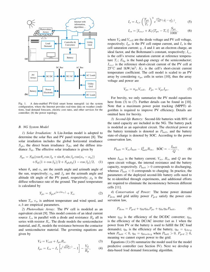
array, a second-life1 lithium-ion battery pack, the home loaddemand, the utility grid, various power converters, data-basedinformation and energy management algorithms. The batteryis necessary to reconcile the imbalance between available PVpower and load demand. The power flow topology is detailedin Fig. 1-(b). The PV panels and the battery are coupled toa DC bus to power DC loads. The DC bus is also connectedto a DC/AC inverter to power AC loads and interact withthe grid. Note that we assume energy will not be exportedto the grid, since a robust regulation for selling electricity tothe grid is absent yet. Compared with conventional homes,the PV-battery smart home NG provides additional degreesof freedom for electric power flow.

The controller’s role is to manage power flow betweenthese components to minimize objectives such as electricitycost or grid power plant emissions, subject to safe operatingconstraints. Specifically, a predictive scheme is applied thatleverages Internet-based data to forecast home load demandand PV power. Next we detail sub-models for the NGcomponents.

1the battery pack is reused from an automotive application, such as anelectric vehicle

Internet with

information,

algorithms ...Photovoltaic

Arrays

Utility

Grid

Controller &

Converters

Battery

Load

Demand

BatteryPower

Electronic

PV

ArraysDC/DC

DC Bus AC Bus

AC Loads

DC Loads

Utility

Grid

DC/AC

(b)

(a)

Fig. 1. A data-enabled PV-Grid smart home nanogrid: (a) the systemconfiguration, where the Internet provides real-time data on weather condi-tions, load demand forecasts, electric cost rates, and other services for thecontroller; (b) the power topology.

B. NG System Model

1) Solar Irradiation: A Liu-Jordan model is adopted todetermine the solar flux and PV panel temperature [8]. Thesolar irradiation includes the global horizontal irradianceSgh, the direct beam irradiance Sdb, and the diffuse irra-diance Sdi. The effective solar irradiance is given by

Spv = Sdb(cos θs cosβp + sin θs sinβp cos(αs − αp))

+Sdi(1 + cosβp)/2 + Sghρg(1− cosβp)/2, (1)

where θs and αs are the zenith angle and azimuth angle ofthe sun, respectively; αp and βp are the azimuth angle andaltitude tilt angle of the PV panel, respectively; ρg is thediffuse reflectance rate of the ground. The panel temperatureis calculated by

Tpv = Spve(a+bvw) + Ta, (2)

where Ta, vw is ambient temperature and wind speed, anda, b are empirical parameters.

2) Photovoltaic Array: The PV cell is modeled as anequivalent circuit [9]. This model consists of an ideal currentsource Ics in parallel with a diode and resistance Rp all inseries with resistor Rs. The diode models the semiconductormaterial, and Rs models the resistance between the contactorand semiconductor material. The governing equations aregiven by

Vd = Vcell + IpvRs, (3)

Ipv = Ics − Is[e

(qVd

AkTpv) − 1

]− VdRp

, (4)

Is = Is,r

(TpvTr

)3

eqEbgAk ( 1

Tr− 1

Tpv), (5)

Ics = [Ics,r +KI(Tpv − Tr)]Spv

1000, (6)

where Vd and Vcell are the diode voltage and PV cell voltage,respectively; Ipv is the PV cell output current, and Is is thecell saturation current; q, A and k are an electron charge, anideal factor, and the Boltzmann’s constant, respectively; Is,ris the cell’s reverse saturation current at reference tempera-ture Tr; Ebg is the band-gap energy of the semiconductor;Ics,r is the reference short-circuit current of the PV cell at25◦C and 1kW/m2; KI is the cell’s short-circuit currenttemperature coefficient. The cell model is scaled to an PVarray by considering npv cells in series [10], thus the arrayvoltage and power are

Vpv = npvVcell, Ppv = VpvIpv. (7)

For brevity, we only summarize the PV model equationshere from (3) to (7). Further details can be found in [10].Note that a maximum power point tracking (MPPT) al-gorithm is required to improve PV efficiency. Details areomitted here for brevity.

3) Second-life Battery: Second-life batteries with 80% ofthe rated capacity are included in the NG. The battery packis modeled as an equivalent circuit. The electrical power atthe battery terminals is denoted as Pbatt, and the batterystate-of-charge is denoted by SOC. According to the powerconservation law,

Pbatt = VocIbatt − I2battRin, ˙SOC = −Ibatt

Q, (8)

where Ibatt is the battery current; Voc, Rin and Q are theopen circuit voltage, the internal resistance and the batterycapacity, respectively. Pbatt > 0 corresponds to discharging,whereas Pbatt < 0 corresponds to charging. In practice, theparameters of the deployed second-life battery cells need tobe re-identified through experiments, and additional effortsare required to eliminate the inconsistency between differentcells [11].

4) Conservation of Power: The home power demandPdem and grid utility power Pgrd satisfy the power con-servation law,

Pdem = Pgrd + ηddηdaPpv + ηdaηbtPbatt, (9)

where ηdd is the efficiency of the DC/DC converter; ηdais the efficiency of the DC/AC inverter (set as 1 when thepower from PV or the battery is used to fulfill the DC loaddemands); ηbt is the efficiency of the battery, ηbt = ηchrgwhen Pbatt < 0, ηbt = ηdischrg when Pbatt > 0. Pgrd ≥ 0,meaning we cannot export power to the grid.

Equations (1)-(9) summarize the model used for the modelpredictive controller (see Section IV). Next we develop adata-based load demand forecasting algorithm.

Apr May Jun Jul Aug Sep Oct Nov Dec Jan Feb Mar

0.5

1

1.5

2

2.5

3

3.5

4

Month

Ele

ctric

ityiL

oadi

HkW

Y

HourlyiLoadDailyiLoadMonthlyiLoadYeariAverage

Fig. 2. Electricity consumption of a single family home in Los Angelesfrom 2013-04-01 to 2014-03-31.

III. DATA ENABLED FORECAST

A. Load Data Analysis

We analyze load data from a single family home inLos Angeles to investigate correlations between the loaddemand and the season, temperature, day of week, and timeof day. The goal is to determine inputs to include in thedata-driven model. The collected data corresponds to daterange 2013-04-01 to 2014-03-31. Figure 2 plots the hourly,daily, monthly and yearly average electricity consumption.The hourly load demand varies between 0.5 kW to 4 kW.The yearly average load is about 1 kW. It is observed thatthe house consumed more energy in August and September(hottest months), and December, January (coldest months)relative to the other months. The correlation between theweekly average load and the weekly average temperatureof this geographical area is also investigated. The resultindicates that more energy is consumed when the weeklyaverage temperature is higher than 21◦C or lower than 14◦C.Since temperature correlates with different seasons, eitherinput can be used for the forecasting model.

The load data is classified according to the day of week,shown in Fig. 3. We can see that from Monday to Thursday,the daily pattern of electricity consumption is similar. Peakloads consistently occur from 7:00 to 8:30 AM, and 6:00 to10:00 PM. On Fridays, the pattern changes. There are twopeak loads observed in the morning, which is clearly differentfrom the Monday-Thursday pattern. During weekends, theelectricity consumption pattern is more random. The peakloads on Saturday and Sunday usually last longer, and thedaytime off-peak load is also higher compared with theweekdays, resulting with a higher average load during theweekend.

This analysis is used to determine the exogenous inputsof the forecast model (to be presented in Section III-B).Note that other information, such as the holidays or personalhabits, can also be incorporated into the forecast model.

B. Load Demand Forecast

A radial basis function neural network (RBF-NN) forecastalgorithm is utilized to forecast short-term future loads. RBF-

Fig. 3. Electric load from Monday to Sunday of the sampled LA data.Blue: load of particular week days; red: hourly average load across allweeks; green: daily average load over all weeks; yellow rectangle: peakload periods.

NN is selected because it captures the nonlinear input-outputrelations of home load demand and achieves reasonable fore-cast accuracy [12]. Please note that other forecast methodsmay be used. Generally, the RBF-NN model contains threelayers: the input layer, the hidden layer, and the output layer.The hidden layer performs nonlinear transforms for featureextraction, and the output layer gives a linear combinationof the output weights. The Gaussian function is used asthe radial basis function in the hidden layer to activate theneurons [5], formulated as

a1 = exp

(−‖ n− c ‖

2

2b2

), (10)

n = Wa0 + b (11)

where a1 and a0 are neural outputs of the current layer andprior layer, respectively; n is accumulator output and W isweight; c is the neural net center and b is the spread width.Both c and b can be fit using a gradient descent method.

Assume the input is X . According to Section III-A, theair temperature, day of week, and time of day are selectedas exogenous inputs to the RBF-NN model, together withthe endogenous input, the historical load. Thus, the input ofthe RBF-NN is designed as X = [Ta Dw Td Lh]T , whereTa is the forecasted air temperature obtained via Internet-based weather services. Ta is the true air temperature andused only during the training process. Dw is the future dayof week. Td is the future time of day. Lh is the historicalload. The output of the forecast algorithm Y is the futurem−dimensional load demand vector, notated as Pdem.

C. Load Demand Forecast Validation

The RBF-NN forecast model is validated in this section.The validation data is one-year real electricity consumptiondata (2013-04-01 to 2014-03-31) collected from two houseslocated in Los Angeles (LA) and Berkeley. The first halfyear data is used for neural network training, and the second

10

20

30° C

0 3 6 9 12 15 18 210

1

2

3

HourAofADayAonA2013 09 15 Tuesday

Load

AbkW

)

10

20

30

0 3 6 9 12 15 18 210

1

2

3

Hour of Day on 2013 12 06 Friday

AirATemperautreAonA09 15

RealALoadForecastAL

AirATemperautreAonA12 06

ba)-1

ba)-2

bb)-1

Fig. 4. Forecast examples and the corresponding air temperature of theLA load data: (a) on 2013-09-15 Tuesday; (b) on 2013-12-06 Friday. Notethat the output vector length is 24-hour, meaning the forecast of the future24-hour loads are completed in one process.

0 0y2 0y4 0y6 0y8 1 1y20

0y2

0y4

0y6

0y8

1

RMSE (kW)

Em

piric

altC

DF

24 21 18 15 12 9 6 3 00y4

0y43

0y46

0y49

0y52

InputtHistoricaltLoadtLength (hour)

Ave

rage

tRM

SE

(kW

)

RMSEtcdftoftLAtDataRMSEtcdftoftBerkeleytData

haA

hbA

Fig. 5. (a): Empirical CDF for forecast RMSE of the LA and Berkeleyload data; (b): Average RMSEs of the LA and Berkeley data with differenthistorical load lengths used in the RBF-NN input (output is 24-hour long).

half year data is used for validation and comparison. Thesampling period of the load data is one hour. The length ofthe historical load (in the input vector) and the length of theprediction horizon (output vector) are both initially set as 24.

An empirical cumulative distribution function (CDF) of allthe root mean square errors (RMSEs) of the forecast resultsare demonstrated in Fig. 5-(a). Note that 80% of the RMSEsare below 0.45 kW and 0.55 kW in the LA and Berkeleydata, respectively. The RBF-NN model is able to maintainthe forecast error within an acceptable range. The accuracyvalidation of the forecast model is further quantified andverified in Section V.

Sensitivity to the input historical load length is alsoinvestigated. The average RMSE of the LA and Berkeleydata with different historical load lengths is illustrated in Fig.5-(b). As expected, longer historical load vectors producebetter forecast accuracy. Interestingly, the marginal accuracyimprovement decreases dramatically for historical load vec-tors greater than six hours. Conversely, the most recent fivehours of load significantly impact forecasting accuracy.

D. Weather, Cost, and Emission Forecasts

Weather forecast services are now ubiquitous from theInternet. We assume that the solar irradiance and air tem-perature information is available via weather forecastingservices (i.e. application programming interfaces (APIs)).The acquired irradiation and temperature information isinjected into the solar irradiation model (see Section II-B.1)to estimate the PV solar flux and PV temperature, denotedas Spv and Tpv , respectively.

In addition, the electric cost and power plant carbonemissions are incorporated into the objective function ofthe controller (see Section IV). This information is alsoassumed to be available from the Internet. The observedelectric rate and unit carbon emission are notated as Re andCe, respectively.

IV. MODEL PREDICTIVE CONTROL

The proposed data-enabled predictive energy managementstrategy determines the optimal power flow, given forecastedload demand, weather conditions, and electricity cost ob-tained from the Internet. Given the system model (1)-(9), werequire one control input to render a casual system, and selectgrid power Pgrd(t). Denoting x(t) as the state variable, u(t)as the control variable, d(t) as the system disturbance, andy(t) as the output, the system model is

x(t) = f(x(t), u(t), d(t)), (12)y(t) = g(x(t), u(t), d(t)), (13)

with x(t) = SOC(t), u(t) = Pgrd(t), y(t) = Pbatt(t).The disturbance d(t) = [Pdem(t), Spv(t), Tpv(t)]T , wherePdem(t), Spv(t), and Tpv(t) are the forecasted load demand,solar irradiation and PV temperature, respectively. The elec-tricity cost and carbon emission can be calculated by

Er(u, t) = Re(t) · u(t), (14)Ec(u, t) = Ce(t) · u(t), (15)

where Re(t) and Ce(t) are time-varying electric rate and unitcarbon emission, respectively. The objective function is

E(u, t) = λ1Er(u, t) + λ2Ec(u, t), (16)

where λ1 and λ2 are weighting parameters. For simplicity,we fix the prediction horizon length equal to the controlhorizon, namely Lp. Assume the time step is ∆t. At timek∆t, the cost function Jk is formulated as

Jk =

∫ (k+Lp)∆t

k∆t

E(u, t)2 dt. (17)

Additionally, the following constraints must be satisfied:

SOCmin ≤ SOC ≤ SOCmax, Iminbatt ≤ Ibatt ≤ Imax

batt ,Pminbatt ≤ Pbatt ≤ Pmax

batt , Pmingrd ≤ Pgrd ≤ Pmax

grd .(18)

Special consideration is given to the battery terminal SOCconstraint during each receding horizon of the MPC. Phys-ically, the battery SOC can vary between SOCmin and

0f40f60f8

1

SO

C

2

0

2

4P

ower

7ykW

G

Monf Tuef Wedf Thuf Frif Satf Sunf15161718

Cen

ts&k

Wh

Load7DemandPV7PowerBattery7PowerGrid7Power

Electric7Rate7from7PGVE

Fig. 6. Week-long control result of the data enabled predictive energymanagement on the LA house when λ1 = 1, λ2 = 0 in cost function (16),with load demand forecast by the RBF-NN.

SOCmax freely. However, in this paper we require theterminal SOC to be equal to a reference value, which is

SOC(k+Lp)∆t = SOC, (19)

where SOC is a pre-defined reference for terminal SOCof each MPC horizon. In this case, the NG works undera charge-sustaining mode, to avoid overcharge or overdis-charge situations. The control procedure of the proposedpredictive energy management strategy follows the standardone of MPC [2].

Dynamic programming (DP) is employed in step twoto solve the constrained nonlinear optimization problemat each time step. Alternative nonlinear formulations thatadmit special structure, e.g. convex programs or quadraticprograms, can utilize corresponding solvers [13]. DP is usedhere for its generality and provable optimality.

V. SIMULATION AND DISCUSSION

A. Data-enabled Predictive Energy Management

The PV panel parameters are adopted from a commercialproduct: Renogy Monocrystalline 250D. The battery packis from a Toyota Prius hybrid electric vehicle, with 168series-arranged C-LiFePO4 cells. Each cell’s nominal chargecapacity is 6.5 Ah, and we assume the second-life pack hasalready degraded to 80% of its original energy capacity. Weconsider 6 PV panels in series and 5 battery packs in parallel.Note that the energy management strategy focuses on slowerdynamics of the NG, thus the control time step is selectedas 1 hour. Faster dynamics are governed by a lower levelcontroller in practice.

1) Supervisory Control: The control and prediction hori-zon length are 24 hours. The electricity load data is collecteddata from single family homes in LA and Berkeley. Theload demand during each control horizon is predicted bythe RBF-NN forecast model. The weather condition, solarflux, electric rate and carbon emission data are obtainedfrom the National Climatic Data Center, PG&E and CAISO,respectively. These information streams are assumed knownto the controller via the Internet.

1 5 9 13 17 21 2555

60

65

70

75

80

85

90

95

100

105

Control%Horizon%Length%(Hour)

Nor

mal

ized

%Cos

t%(P

)

MPC%with%NGDP%OptimalWithout%NG

Fig. 7. Normalized energy management performance when increasing thecontrol horizon length from 1 to 24, where CM stands for the proposed data-enabled predictive energy management strategy. The cost without PV/batteryis normalized as 100% to indicate the worst case performance. Dp optimalis the best-case solution solved by DP when full knowledge is known apriori.

First, we consider λ1 = 1, λ2 = 0 in the cost function(16) to investigate the optimal NG behavior with respect toelectric cost only. A week-long energy management result isshown in Fig. 6. The PV power is intermittent, and dropsto zero during the night. During the day, the solar energy isdirectly used to power the house. Extra energy is stored intothe battery for future use. When solar energy is insufficient tosatisfy load demand, the battery or grid provides support. Thebottom figure shows a two-tiered cost structure, includinghigh-cost “on-peak” rates and lower-cost “off-peak” rates.To reduce the electricity cost, the controller avoids on-peakgrid power as much as possible, as demonstrated in Fig. 6.Consequently the battery generally charges during off-peakperiods, and discharges during on-peak periods.

A similar simulation result is observed where the objectiveis to minimize the carbon emissions Ec, i.e. λ1 = 0, λ2 = 1.The controller avoids using grid power during higher carbon-emission periods.

2) Horizon Length Determination: Next we examine con-trol horizon length. The energy management performance forcontrol horizons of 1 hr. to 25 hrs. are shown in Fig. 7,normalized to the electric cost without PV and battery (i.e.without NG). For a 1 hr. horizon, the MPC is short-sightedand normalized cost is about 85%. As the control lengthincreases, the performance converges towards the lowerbound calculated via dynamic programming (DP) with globaltime horizon and perfect forecasts (DP optimal). When thecontrol length is 7 hours, the cost is 2% greater than theDP result (approximately 64%). Consequently, performancenearly equal to having perfect forecasts (i.e. the DP result)can be achieved with a 7 hour horizon, with negligiblemarginal improvements for longer control horizons.

3) Energy Manager Assessment: Ten weeks are randomlyselected from the LA and Berkeley data sets for a com-prehensive assessment of the controller. Results are listedin Table I. Symbols C, P and σ indicate the cost orcarbon in USD or kg, percentage, and the standard deviation,

TABLE IPERFORMANCE COMPARISON WITH RESPECT TO COST AND CARBON

Type Crt Prt σrt Ccb Pcb σcb

Without NG 27.32 100% – 8.03 100% –DP with NG 16.97 62.1% +/-0.3% 4.93 61.4% +/-0.7%CM with NG 17.54 64.2% +/-0.8% 5.07 63.1% +/-1.2%

(rt indicated for the electric rate, and cb means the carbon emission.)

0 0.1 0.2 0.3 0.4 0.5 0.6 0.7 0.8 0.9

62

64

66

68

70

72

LoadiDemandiForecastiRMSE

Nor

mal

ized

iCos

tip)

U

DPiOptimalUniformiDistributionRBF−NNiResult

Fig. 8. Normalized energy management performance of the artificiallyformulated load demand with uniformly distributed RMSEs from 0 to 1,compared with the RBF-NN energy management results.

respectively. We can see that both the electricity cost andcarbon emission can be reduced by over 35% compared tohomes without a NG system. Moreover, the data-enabledpredictive energy management is only 2% worse than the DPoptimal benchmark. This suggests moderately accurate fore-casts of load demand are sufficient for excellent controller

4) Forecast Error Sensitivity Study: Next we investi-gate load demand forecasting error on energy managementperformance. To conduct this sensitivity study, we appenduniformly distributed random errors to the real load demanddata. The RMSE of this artificially formulated load is in-creased from 0 to 1 (kW). We implant the contaminated loaddemand forecasts into the MPC.

Over 200 tests with uniformly distributed errors are con-ducted, compared with 20 RBF-NN tests, shown in Fig.8. When the RMSE is below 0.3 kW, the energy managerperforms closely to the DP optimal solution, with normalizedcosts are between 62% and 64% compared with no NGscenario. These results demonstrate that normalized costincreases linearly as the forecast RMSE increases.

Additionally, we note the RMSE of the RBF-NN fore-caster is near 0.38 kW. The normalized cost is 63.4%, whichequals the performance of contaminated forecasts with just0.25 kW RMSE. This result is surprisingly good, whichis only 1.5-2% higher than the DP optimal solution. Aftercomparison, we found that the forecast RMSE produced bythe RBF-NN has a tighter distribution (i.e. smaller variance)compared to uniformly distributed errors. This indicatesthat the RBF-NN forecast model captures the nonlinear

performance.characteristics of the load data and provides a reasonabledisturbance estimate for MPC, relative to the performanceachieved with perfect forecasts.

VI. CONCLUSIONS

This paper presents a data enabled predictive energy man-agement strategy for a PV-battery smart home nanogrid. Amodel predictive controller (MPC) is formulated to solve theenergy management problem. A RBF-NN model is utilizedto forecast home load demand, which is used as a disturbanceprediction in the MPC controller. Future weather conditionsand other information streams are acquired from the Internetintegrated into the energy management system. Numericalexperiments demonstrate that the proposed predictive energymanagement system achieves 96%-98% optimality of thedeterministic DP benchmark with respect to electric cost andcarbon emission. In addition, the controller’s sensitivity tothe control horizon length and load demand forecast accuracyare investigated to determine the fundamental tradeoffs. Fu-ture work involves energy storage from plug-in electric vehi-cles, and demonstration of the proposed energy managementstrategy on an experimental smart home at the University ofCalifornia, Davis [11].

REFERENCES

[1] N. Hatziargyriou, H. Asano, R. Iravani, and C. Marnay, “Microgrids,”IEEE Power and Energy Magazine, vol. 5, no. 4, pp. 78–94, 2007.

[2] E. F. Camacho and C. B. Alba, Model Predictive Control. Springer,2013.

[3] A. Chaouachi, R. M. Kamel, R. Andoulsi, and K. Nagasaka, “Mul-tiobjective intelligent energy management for a microgrid,” IEEETransactions on Industrial Electronics, vol. 60, no. 4, pp. 1688–1699,2013.

[4] E. Perez, H. Beltran, N. Aparicio, and P. Rodriguez, “Predictive powercontrol for PV plants with energy storage,” IEEE Transactions onSustainable Energy, vol. 4, no. 2, pp. 482–490, 2013.

[5] H. S. Hippert, C. E. Pedreira, and R. C. Souza, “Neural networksfor short-term load forecasting: A review and evaluation,” IEEETransactions on Power Systems, vol. 16, no. 1, pp. 44–55, 2001.

[6] Y. Suhara, T. Nakabe, G. Mine, and H. Nishi, “Distributed demand sidemanagement system for home energy management,” in 36th AnnualConference on IEEE Industrial Electronics Society. IEEE, 2010, pp.2430–2435.

[7] D. Zhang, L. G. Papageorgiou, N. J. Samsatli, and N. Shah, “Optimalscheduling of smart homes energy consumption with microgrid,” inThe First International Conference on Smart Grids, Green Communi-cations and IT Energy-aware Technologies, 2011, pp. 70–75.

[8] B. Liu and R. Jordan, “Daily insolation on surfaces tilted towardsequator,” ASHRAE J. (United States), vol. 10, 1961.

[9] G. Vachtsevanos and K. Kalaitzakis, “A hybrid photovoltaic simulatorfor utility interactive studies,” IEEE Transactions on Energy Conver-sion, no. 2, pp. 227–231, 1987.

[10] S. J. Moura and Y. A. Chang, “Lyapunov-based switched extremumseeking for photovoltaic power maximization,” Control EngineeringPractice, vol. 21, no. 7, pp. 971–980, 2013.

[11] S. J. Tong, A. Same, M. A. Kootstra, and J. W. Park, “Off-gridphotovoltaic vehicle charge using second life lithium batteries: Anexperimental and numerical investigation,” Applied Energy, vol. 104,pp. 740–750, 2013.

[12] N. Amjady, “Short-term hourly load forecasting using time-seriesmodeling with peak load estimation capability,” IEEE Transactionson Power Systems, vol. 16, no. 3, pp. 498–505, 2001.

[13] S. Boyd and L. Vandenberghe, Convex optimization. Cambridge university press, 2009.