Data-driven System Design in Service Operations System Design in Service Operations ... These...

Data-driven System Design in Service Operations

Yina Lu

Submitted in partial fulfillment of the

requirements for the degree of

Doctor of Philosophy

under the Executive Committee

of the Graduate School of Arts and Sciences

COLUMBIA UNIVERSITY

2013

c©2013

Yina Lu

All Rights Reserved

ABSTRACT

Data-driven System Design in Service Operations

Yina Lu

The service industry has become an increasingly important component in the world’s econ-

omy. Simultaneously, the data collected from service systems has grown rapidly in both size and

complexity due to the rapid spread of information technology, providing new opportunities and

challenges for operations management researchers. This dissertation aims to explore methodolo-

gies to extract information from data and provide powerful insights to guide the design of service

delivery systems. To do this, we analyze three applicationsin the retail, healthcare, and IT service

industries.

In the first application, we conduct an empirical study to analyze how waiting in queue in the

context of a retail store affects customers’ purchasing behavior. The methodology combines a

novel dataset collected via video recognition technology with traditional point-of-sales data. We

find that waiting in queue has a nonlinear impact on purchase incidence and that customers appear

to focus mostly on the length of the queue, without adjustingenough for the speed at which the

line moves. We also find that customers’ sensitivity to waiting is heterogeneous and negatively

correlated with price sensitivity. These findings have important implications for queueing system

design and pricing management under congestion.

The second application focuses on disaster planning in healthcare. According to a U.S. govern-

ment mandate, in a catastrophic event, the New York City metropolitan areas need to be capable

of caring for 400 burn-injured patients during a catastrophe, which far exceeds the current burn

bed capacity. We develop a new system for prioritizing patients for transfer to burn beds as they

become available and demonstrate its superiority over several other triage methods. Based on data

from previous burn catastrophes, we study the feasibility of being able to admit the required num-

ber of patients to burn beds within the critical three-to-five-day time frame. We find that this is

unlikely and that the ability to do so is highly dependent on the type of event and the demographics

of the patient population. This work has implications for how disaster plans in other metropolitan

areas should be developed.

In the third application, we study workers’ productivity ina global IT service delivery system,

where service requests from possibly globally distributedcustomers are managed centrally and

served by agents. Based on a novel dataset which tracks the detailed time intervals an agent spends

on all business related activities, we develop a methodology to study the variation of productiv-

ity over time motivated by econometric tools from survival analysis. This approach can be used

to identify different mechanisms by which workload affectsproductivity. The findings provide

important insights for the design of the workload allocation policies which account for agents’

workload management behavior.

Contents

List of Figures v

List of Tables vii

Acknowledgements x

1 Introduction 1

1.1 Overview . . . . . . . . . . . . . . . . . . . . . . . . . . . . . . . . . . . . . . . 1

1.1.1 Elements in a Service Delivery System . . . . . . . . . . . . . .. . . . . 2

1.1.2 Data-driven Decision Making . . . . . . . . . . . . . . . . . . . . .. . . 4

1.2 Outline . . . . . . . . . . . . . . . . . . . . . . . . . . . . . . . . . . . . . . . . 6

2 Measuring the Effect of Queues on Customer Purchases 9

2.1 Introduction . . . . . . . . . . . . . . . . . . . . . . . . . . . . . . . . . . . .. . 9

2.2 Related Work . . . . . . . . . . . . . . . . . . . . . . . . . . . . . . . . . . . . .13

2.3 Estimation . . . . . . . . . . . . . . . . . . . . . . . . . . . . . . . . . . . . . .. 18

2.3.1 Data . . . . . . . . . . . . . . . . . . . . . . . . . . . . . . . . . . . . . . 19

i

2.3.2 Purchase Incidence Model . . . . . . . . . . . . . . . . . . . . . . . .. . 22

2.3.3 Inferring Queues From Periodic Data . . . . . . . . . . . . . . .. . . . . 27

2.3.4 Outline of the Estimation Procedure . . . . . . . . . . . . . . .. . . . . . 33

2.3.5 Simulation Test . . . . . . . . . . . . . . . . . . . . . . . . . . . . . . . .35

2.3.6 Choice Model . . . . . . . . . . . . . . . . . . . . . . . . . . . . . . . . . 36

2.4 Empirical Results . . . . . . . . . . . . . . . . . . . . . . . . . . . . . . . .. . . 42

2.4.1 Purchase Incidence Model Results . . . . . . . . . . . . . . . . .. . . . 43

2.4.2 Choice Model results . . . . . . . . . . . . . . . . . . . . . . . . . . . .. 48

2.5 Managerial Implications . . . . . . . . . . . . . . . . . . . . . . . . . .. . . . . 51

2.5.1 Queuing Design . . . . . . . . . . . . . . . . . . . . . . . . . . . . . . . 51

2.5.2 Implications for Staffing Decision . . . . . . . . . . . . . . . .. . . . . . 53

2.5.3 Implications for Category Pricing . . . . . . . . . . . . . . . .. . . . . . 55

2.6 Conclusions . . . . . . . . . . . . . . . . . . . . . . . . . . . . . . . . . . . . .. 59

3 Prioritizing Burn-Injured Patients During a Disaster 62

3.1 Introduction . . . . . . . . . . . . . . . . . . . . . . . . . . . . . . . . . . . .. . 62

3.2 Background . . . . . . . . . . . . . . . . . . . . . . . . . . . . . . . . . . . . . .66

3.2.1 Burn Care . . . . . . . . . . . . . . . . . . . . . . . . . . . . . . . . . . . 66

3.2.2 Disaster Plan . . . . . . . . . . . . . . . . . . . . . . . . . . . . . . . . . 67

3.2.3 Operations Literature . . . . . . . . . . . . . . . . . . . . . . . . . .. . . 72

3.3 Model and a Heuristic . . . . . . . . . . . . . . . . . . . . . . . . . . . . . .. . . 74

3.3.1 Potential Triage Policies . . . . . . . . . . . . . . . . . . . . . . .. . . . 76

ii

3.3.2 Proposed Heuristic . . . . . . . . . . . . . . . . . . . . . . . . . . . . .. 77

3.4 Parameter Estimation and Model Refinement . . . . . . . . . . . .. . . . . . . . 80

3.4.1 Parameter Estimation . . . . . . . . . . . . . . . . . . . . . . . . . . .. . 80

3.4.2 Inclusion of Patient Comorbidities . . . . . . . . . . . . . . .. . . . . . . 85

3.4.3 Summary of Proposed Triage Algorithm . . . . . . . . . . . . . .. . . . . 88

3.5 Evaluating the Algorithm . . . . . . . . . . . . . . . . . . . . . . . . . .. . . . . 89

3.5.1 Data Description . . . . . . . . . . . . . . . . . . . . . . . . . . . . . . .90

3.5.2 Simulation Scenarios . . . . . . . . . . . . . . . . . . . . . . . . . . .. . 92

3.5.3 Simulation Results: Unknown Comorbidities . . . . . . . .. . . . . . . . 93

3.5.4 Simulation Results: Comorbidities . . . . . . . . . . . . . . .. . . . . . . 94

3.5.5 Performance of the Proposed Triage Algorithm . . . . . . .. . . . . . . . 97

3.6 Feasibility . . . . . . . . . . . . . . . . . . . . . . . . . . . . . . . . . . . . .. . 100

3.6.1 Clearing Current Patients . . . . . . . . . . . . . . . . . . . . . . .. . . . 102

3.7 Conclusions and Discussion . . . . . . . . . . . . . . . . . . . . . . . .. . . . . 104

4 The Design of Service Delivery Systems with Workload-dependent Service Rates 108

4.1 Introduction . . . . . . . . . . . . . . . . . . . . . . . . . . . . . . . . . . . .. . 108

4.2 Background and Data . . . . . . . . . . . . . . . . . . . . . . . . . . . . . . .. 112

4.2.1 Overview of the Service Delivery Process . . . . . . . . . . .. . . . . . . 112

4.2.2 Data Collection . . . . . . . . . . . . . . . . . . . . . . . . . . . . . . . .115

4.2.3 Sample Selection and Summary Statistics . . . . . . . . . . .. . . . . . . 118

4.3 Econometric Model of Agent’s Productivity . . . . . . . . . . .. . . . . . . . . . 120

iii

4.3.1 Measuring Productivity . . . . . . . . . . . . . . . . . . . . . . . . .. . . 121

4.3.2 Factors Influencing Productivity . . . . . . . . . . . . . . . . .. . . . . . 123

4.4 Estimation Results . . . . . . . . . . . . . . . . . . . . . . . . . . . . . . .. . . 130

4.5 Impact of Workload on Request Allocation Policies . . . . .. . . . . . . . . . . . 136

4.6 Accounting for Agent’s Priority Schemes . . . . . . . . . . . . .. . . . . . . . . 141

4.6.1 Agent Choice Model . . . . . . . . . . . . . . . . . . . . . . . . . . . . . 141

4.6.2 Impact of Processing Order on Request Allocation Policies . . . . . . . . 143

4.7 Conclusion . . . . . . . . . . . . . . . . . . . . . . . . . . . . . . . . . . . . . .146

Bibliography 156

A Appendix for Chapter 2 157

A.1 Determining the Distribution for Deli Visit Time . . . . . .. . . . . . . . . . . . . 157

B Appendix for Chapter 3 160

B.1 Simulation Model . . . . . . . . . . . . . . . . . . . . . . . . . . . . . . . . .. . 160

B.2 Inhalation Injury Summary . . . . . . . . . . . . . . . . . . . . . . . . .. . . . . 162

B.3 Arrival Patterns of Burn-Injured Patients to NY Presbyterian . . . . . . . . . . . . 162

B.4 Resources for Prevalence Data . . . . . . . . . . . . . . . . . . . . . .. . . . . . 163

C Appendix for Chapter 4 164

C.1 Data Linking and Cleaning . . . . . . . . . . . . . . . . . . . . . . . . . .. . . . 164

C.2 Impact of Workload on Interruptions . . . . . . . . . . . . . . . . .. . . . . . . . 167

iv

List of Figures

1.1 The links in the service-profit chain from Heskett et al. (1994) . . . . . . . . . . . 2

2.1 Example of a deli snapshot showing the number of customers waiting (left) and

the number of employees attending (right). . . . . . . . . . . . . . .. . . . . . . . 20

2.2 Sequence of events related to a customer purchase transaction. . . . . . . . . . . . 27

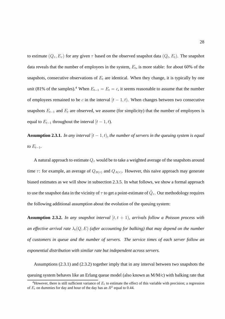
2.3 Estimates of the distribution of the queue length observed by a customer for differ-

ent deli visit times (τ ). The previous snapshot is att = 0 and shows 2 customers

in queue. . . . . . . . . . . . . . . . . . . . . . . . . . . . . . . . . . . . . . . . 32

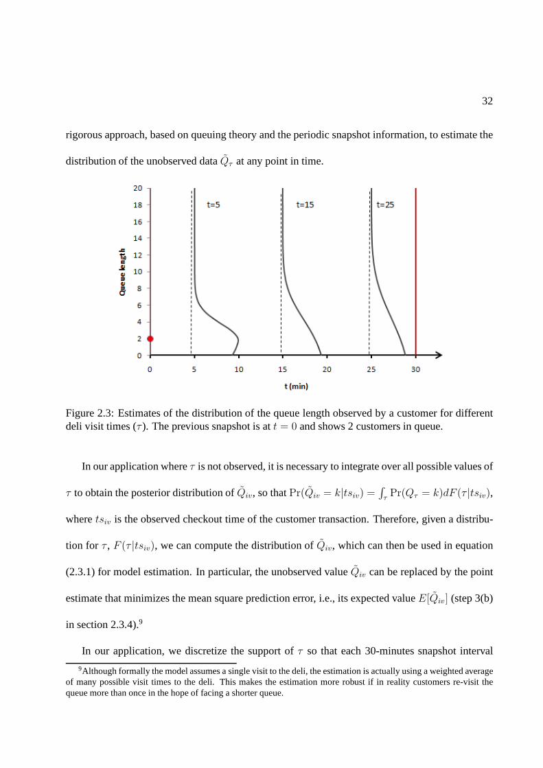
2.4 Estimation results of the purchase incidence model using simulated data. . . . . . . 37

2.5 Results from three different specifications of the purchase incidence model. . . . . 45

2.6 Purchase probability of ham products in the deli sectionversus queue length for

three customer segments with different price sensitivity.. . . . . . . . . . . . . . . 50

2.7 Comparison between the Split Join-Shortest-Queue (JSQ) and Pooled systems. . . 54

3.1 Timeline for care of burn-injured patients: from Wang (2010) and private commu-

nications. . . . . . . . . . . . . . . . . . . . . . . . . . . . . . . . . . . . . . . . 67

3.2 Burn Disaster Receiving Hospital triage matrix as reported in Yurt et al. (2008) . . 71

v

3.3 Relative Improvement of Average Additional Survivors .. . . . . . . . . . . . . . 94

3.4 Relative Improvement of Average Increase in Number of Survivors due to Tier 1

treatment: Proposed-W versus Proposed-N . . . . . . . . . . . . . . .. . . . . . . 98

3.5 Relative Improvement of Average Increase in Number of Survivors due to Tier 1

treatment: Proposed-W versus Original . . . . . . . . . . . . . . . . .. . . . . . 99

3.6 Feasibility: Number of beds fixed at 210 . . . . . . . . . . . . . . .. . . . . . . 101

3.7 Feasibility: Number of patients fixed at 400 . . . . . . . . . . .. . . . . . . . . . 103

4.1 Flowchart of the service delivery process . . . . . . . . . . . .. . . . . . . . . . 115

4.2 Plot of impact of size of agent’s personal queue on agent’s productivity (dashed

lines represent the 95% confidence interval) . . . . . . . . . . . . .. . . . . . . . 132

4.3 Productivity variation at different times of a shift (dash lines represent the 95%

confidence interval) . . . . . . . . . . . . . . . . . . . . . . . . . . . . . . . . .. 134

B.1 Monthly and Day-of-week arrival pattern in NYP data set .. . . . . . . . . . . . 162

C.1 Example: Determining the shift schedule for a representative agent . . . . . . . . 166

vi

List of Tables

2.1 Summary statistics of the snapshot data, point-of-sales data and loyalty card data. . 22

2.2 Statistics for the ten most popular ham products, as measured by the percent of

transactions in the category accounted by the product (Share). Prices are measured

in local currency per kilogram (1 unit of local currency = US$21, approximately). . 39

2.3 Goodness of fit results on alternative specifications of the purchase incidence model

(equation (2.3.1)). . . . . . . . . . . . . . . . . . . . . . . . . . . . . . . . . .. . 43

2.4 MLE results for purchase incidence model (equation (2.3.1)) . . . . . . . . . . . . 44

2.5 Estimation results for the choice model (equation 2.3.2). The estimate and standard

error (s.e.) of each parameter correspond to the mean and standard deviation of its

posterior distribution. . . . . . . . . . . . . . . . . . . . . . . . . . . . . .. . . 48

2.6 Cross-price elasticities describing changes in the probability of purchase of the

high price product (H) from changes in the price of the low price product (L). . . . 58

3.1 Patient parameters for three patient, one bed example . .. . . . . . . . . . . . . . 79

3.2 TIMM coefficients as reported in Osler et al. (2010) . . . . .. . . . . . . . . . . . 81

vii

3.3 Approximate range of survival probability and deterioration weights for different

types of patients . . . . . . . . . . . . . . . . . . . . . . . . . . . . . . . . . . . .83

3.4 Mean patient length-of-stay and standard deviation forburn-injured patients grouped

by burn size and survival outcome as summarized from (American Burn Associa-

tion 2009). . . . . . . . . . . . . . . . . . . . . . . . . . . . . . . . . . . . . . . . 84

3.5 Summary of how model parameters are assigned to patients. Deterioration weights

wi are listed as the values used for most results. Ranges for these values can be

found in Table 3.3. . . . . . . . . . . . . . . . . . . . . . . . . . . . . . . . . . . 85

3.6 Odds Ratio (OR), Transform Coefficient (TC), and prevalence of various Comor-

bidities as reported in Thombs et al. (2007) and others. Prevalence is given for the

American Burn Associate National Burn Repository (ABA-NBR), while for New

York City and the United States, it is given for the general population. When it is

specified by age, the age group is listed after the separationbar, i.e. the prevalence

for Peripheral Vascular Disorder is given for people aged 50and older. . . . . . . . 87

3.7 Triage Index. Higher index corresponds to higher priority for a Tier 1 bed. . . . . 90

3.8 Distribution of age, severity of burn (TBSA), and inhalation injury (when known)

in burn data as summarized from Yurt et al. (2005), Chim et al.(2007), Mahoney

et al. (2005). . . . . . . . . . . . . . . . . . . . . . . . . . . . . . . . . . . . . . . 91

3.9 Distribution of age, severity of burn (TBSA), and inhalation injury for four simu-

lation scenarios. . . . . . . . . . . . . . . . . . . . . . . . . . . . . . . . . . . .. 93

3.10 Scenario Statistics . . . . . . . . . . . . . . . . . . . . . . . . . . . . .. . . . . . 93

viii

3.11 Impact of comorbidity information: Relative improvement and standard error in

percentages. . . . . . . . . . . . . . . . . . . . . . . . . . . . . . . . . . . . . . 97

4.1 Sample of Timing Data for a request that is completed in three sessions, each

column represents a session. . . . . . . . . . . . . . . . . . . . . . . . . . .. . . 117

4.2 Summary statistics of the explanatory variables . . . . . .. . . . . . . . . . . . . 130

4.3 Estimation results of the cox proportional hazard rate model. Standard errors in

parenthesis. Stars indicate the significance level, *** for0.01, ** for 0.05, and *

for 0.1. . . . . . . . . . . . . . . . . . . . . . . . . . . . . . . . . . . . . . . . . . 131

4.4 Numerical example 1: Service capacity required to meet SLA’s . . . . . . . . . . 140

4.5 Estimation results of the agent choice model . . . . . . . . . .. . . . . . . . . . 144

4.6 Numerical example 2: Service capacity required to meet SLA’s . . . . . . . . . . 146

A.1 Regression results for the deli visit time distribution. (* p < 0.1 , ** p < 0.05 ) . . 159

B.1 Fraction of patients with Inhalation Injury in the National Burn Repository dataset

as summarized from Osler et al. (2010). . . . . . . . . . . . . . . . . . .. . . . . 162

B.2 Resources for prevalence data. . . . . . . . . . . . . . . . . . . . . .. . . . . . . 163

C.1 The impact of workload on interruption frequency: summary statistics and regres-

sion coefficients . . . . . . . . . . . . . . . . . . . . . . . . . . . . . . . . . . . .168

C.2 The impact of workload on interruption length: summary statistics and regression

coefficients. Stars indicate the significance level, ** for 0.05, and * for 0.1 . . . . . 169

ix

Acknowledgements

My deepest gratitude goes to my advisors Professor Marcelo Olivares and Professor Linda

Green. It is my honor to work with them. I would not have accomplished this without their

continuous guidance and encouragement throughout the years.

I am grateful to Professor Andres Musalem, Professor Carri Chan, and Aliza Heching for their

invaluable help and advices on my thesis chapters. It was my pleasure to work with them. I also

owe my heartfelt appreciation to Professor Awi Federgruen,Professor Andres Musalem, and Aliza

Heching for serving on my defense committee.

Last but not the least, I would like to give my special thank tomy husband Xingbo Xu, whom

I met here at Columbia, and my parents Zhiqing He and Yunian Lu. Their love and support

throughout these years gave me the strength to overcome hardtimes.

x

To Xingbo, Zhiqing, and Yunian

xi

1

Chapter 1

Introduction

1.1 Overview

The service industry has become an increasingly important component in the world’s economy, ac-

counting for more than 60% of the world’s GDP in year 2012 (Agency (2012), Kenessey (1987)).

The service industry involves the provision of services to businesses as well as final consumers.

It is broad in scope, covering transportation, retail, healthcare, entertainment, financial services,

insurance, tourism, and communications. With the rapid growth of the service industry and in-

formation technology, the data collected from service delivery systems has also been exploding.

These datasets provide great opportunities for operationsmanagement researchers to study the

links in service delivery systems. This dissertation aims to explore methodologies to extract in-

formation from the data and provide powerful insights to guide the design of the service delivery

system.

2

This section provides an overview of the elements in a service delivery system and the data-

driven methodologies one can apply to understand the links among these elements.

1.1.1 Elements in a Service Delivery System

The management and design of service delivery systems have always been an important topic

in operations management. With the rapid growth of the service industry, the focus of service

operations management has shifted gradually from purely pursuing market share and profit targets

to the more fundamental elements in the service chain: the customer, the employee, and their

interaction with the design of the service delivery process. The inherent relationships among these

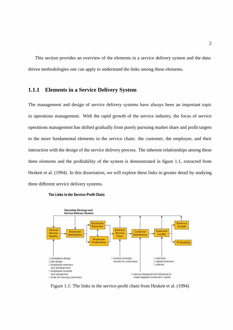
three elements and the profitability of the system is demonstrated in figure 1.1, extracted from

Heskett et al. (1994). In this dissertation, we will explorethese links in greater detail by studying

three different service delivery systems.

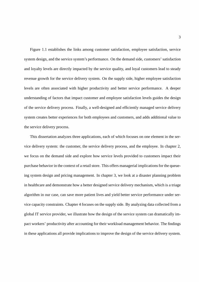
Figure 1.1: The links in the service-profit chain from Heskett et al. (1994)

3

Figure 1.1 establishes the links among customer satisfaction, employee satisfaction, service

system design, and the service system’s performance. On thedemand side, customers’ satisfaction

and loyalty levels are directly impacted by the service quality, and loyal customers lead to steady

revenue growth for the service delivery system. On the supply side, higher employee satisfaction

levels are often associated with higher productivity and better service performance. A deeper

understanding of factors that impact customer and employeesatisfaction levels guides the design

of the service delivery process. Finally, a well-designed and efficiently managed service delivery

system creates better experiences for both employees and customers, and adds additional value to

the service delivery process.

This dissertation analyzes three applications, each of which focuses on one element in the ser-

vice delivery system: the customer, the service delivery process, and the employee. In chapter 2,

we focus on the demand side and explore how service levels provided to customers impact their

purchase behavior in the context of a retail store. This offers managerial implications for the queue-

ing system design and pricing management. In chapter 3, we look at a disaster planning problem

in healthcare and demonstrate how a better designed servicedelivery mechanism, which is a triage

algorithm in our case, can save more patient lives and yield better service performance under ser-

vice capacity constraints. Chapter 4 focuses on the supply side. By analyzing data collected from a

global IT service provider, we illustrate how the design of the service system can dramatically im-

pact workers’ productivity after accounting for their workload management behavior. The findings

in these applications all provide implications to improve the design of the service delivery system.

4

1.1.2 Data-driven Decision Making

The datasets collected from service systems have grown rapidly in both size and complexity due

to the rapid spread of information technology in recent years. It has been estimated that 90% of

the data in the world today has been created in the last two years alone (Frank (2012)). The data

collected from service systems not only grows in its size, but also in its variety. We now summarize

several types of data sources that are commonly used in operations management studies.

Depending on the purpose of its collection, data is classified into primary and secondary data.

Primary data are collected by the researcher for the purposeof the study, whereas secondary data

are collected by other institutes and re-used by researchers. Primary data typically provides more

tailored information, but it is often more expensive to obtain than secondary data. Data can also

be classified depending on its collection method, which includes system operational data, exper-

iments, surveys, interviews, etc. Different data collection methods have their pros and cons. For

example, operational data is typically systematically collected by the service delivery system. It is

a good resource to study the performance of the service delivery system over a long period. Field

or laboratory experiments are expensive to conduct, but they are powerful tools to test hypotheses

and validate model predictions. Survey data is prone to errors, but it tracks information of people’s

subjective opinions. Finally, data also has different origins and sources. Nowadays information

can be obtained through new sources such as smartphones, video cameras, websites, and social

media platforms. All of these data provide new resources foroperations management researchers

with both opportunities and challenges.

The opportunities lie in the potential to unveil the embedded information in these data sources.

5

Traditional operations research efforts typically focus on the development of analytic models with-

out substantial practical support. There typically has been no data available to inform or validate

model assumptions and predictions, or provide insights that may give rise to model refinements

or the need for new models. New data sources provide great opportunities to overcome this de-

ficiency. For empirical researchers in operations management, the analysis of these datasets can

be used to develop policy insights and operational methodologies to improve the effectiveness and

efficiency of the service delivery process. As a good example, Gans et al. (2003) illustrates how the

analysis of real operational data helps to validate model assumptions and motivate model refine-

ments in the context of call centers, a field which is traditionally modeling-oriented. This synergy

between empirical and theoretical methodologies strengthens the usefulness of both.

On the other hand, data-driven methodologies can be costly.Collecting primary data is ex-

pensive; additional efforts are required to link data from different sources; and special techniques

are needed to handle large datasets. The challenge is sometime methodological. When classical

statistical and econometric methodologies are not adequate, a more structured approach needs to

be developed to unveil the embedded information in the data.These methodologies are valuable to

serve as a vehicle for bringing analytical models to practical uses.

A common feature of the studies in this dissertation is that they are motivated and supported

by the analysis of various datasets. In chapter 2, we analyzea novel dataset which was collected

at a supermarket using automatic digital cameras and image recognition technology. We combine

this novel dataset with traditional store transaction datato study customers’ purchase behavior.

The major challenge in this study lies in inferring the stateof the service system from such peri-

odic store operational data. We overcome this by developinga rigorous approach by combining

6

analytical models of the underlying stochastic system witheconometric tools. In chapter 3, the

study is based on secondary data. We first refine the existing empirical models to predict a burn

patient’s survival probability and length-of-stay based on historical burn patients’ treatment data.

These empirical findings motivate us to develop a new heuristic triage plan, which we compare

with existing plans using a simulation based on data from previous burn catastrophes. In chapter

4, a novel dataset was collected with the purpose of studyingagent’s behavior in managing their

workload. This novel dataset is then linked with other operational data, enabling us to develop a

new measure of worker’s productivity. We use this approach to identify different mechanisms by

which workload affects productivity, which is challengingto measure using traditional productiv-

ity measures such as throughput rates and service times. In all these studies, various types of data

collected in the service delivery process play an importantrole in providing insights for the service

system design.

1.2 Outline

The rest of the dissertation is organized as follows.

Chapter 2 studies how waiting in queue in the context of a retail store affects customers pur-

chasing behavior using real-time store operational and transaction data. The major challenge in

this study lies in the periodic nature of the store operational data collected using the image recog-

nition technology and digital camera shots which makes it difficult to infer the queue length that

each customer encounters. We overcome this by developing a rigorous approach that infers these

missing data by modeling the transient behavior of the underlying stochastic process of the queue.

7

The analytical model is then combined with econometric tools to estimate customers’ responses,

and a simulation study is conducted to validate the estimation methodology. Our empirical finding

suggests that waiting in queue has a non-linear impact on purchase decisions and that customers

appear to focus mostly on the length of the queue, without accounting for the service speed. We

also find that customers sensitivity to waiting is heterogeneous and negatively correlated with price

sensitivity. We then discuss the implications of these results for queuing design, staffing, and cate-

gory pricing.

Chapter 3 focuses on disaster planning in healthcare. It is motivated by the U.S. government

mandate that, in a catastrophic event, metropolitan areas need to be capable of caring for 50 burn-

injured patients per million population. This mandate translates into 400 patients in New York

City, while the current burn bed capacity is only 210. To address this gap, we were asked by the

NYC Burn Disaster Plan Working Group to develop a new system for prioritizing burn patients

to maximize the number of survivors given limited bed capacities. To do this, we first refine the

existing models to predict a burn patient’s survival probability and length-of-stay more accurately

based on factors including age, burn size, inhalation injury, and co-morbidities. The empirical

findings of how patient characteristics impact length-of-stay and survivability also motivated the

a new heuristic we developed for prioritizing patients for transfer to burn beds which we show is

superior to several other triage methods. By simulating thenumber of survivors and bed turnovers

under different scenarios based on data from previous burn catastrophes, we also demonstrate that

the current burn bed capacity in NYC is unlikely to be sufficient to conform to the federal mandate.

This work has implications for how disaster plans in other metropolitan areas should be developed.

Chapter 4 investigates factors that impact worker’s productivity in a global IT service delivery

8

system, where service requests from possibly globally distributed customers are managed centrally

and served by agents. In order to identify desirable features of the request allocation and workload

management policy for the dispatcher, we study the link between request allocation policies and

the performance of the service system. Based on a novel dataset which tracks the detailed time

intervals an agent spends on all business related activities, we develop a methodology to study the

variation of productivity over time motivated by econometric tools from survival analysis. This

approach can be used to identify different mechanisms by which workload affects productivity.

The identification of these mechanisms provides interesting insights for the design of the workload

allocation policy.

9

Chapter 2

Measuring the Effect of Queues on

Customer Purchases

2.1 Introduction

Capacity management is an important aspect in the design of service operations. These decisions

involve a trade-off between the costs of sustaining a service level standard and the value that

customers attach to it. Most work in the operations management literature has focused on the

first issue developing models that are useful to quantify thecosts of attaining a given level of

service. Because these operating costs are more salient, itis frequent in practice to observe service

operations rules designed to attain a quantifiable target service level. For example, a common rule

in retail stores is to open additional check-outs when the length of the queue surpasses a given

threshold. However, there isn’t much research focusing on how to choose an appropriate target

service level. This requires measuring the value that customers assign to objective service level

10

measures and how this translates into revenue. The focus of this study is to measure the effect of

service levels– in particular, customers waiting in queue–on actual customer purchases, which can

be used to attach an economic value to customer service.

Lack of objective data is an important limitation to study empirically the effect of waiting on

customer behavior. A notable exception is call centers, where some recent studies have focused

on measuring customer impatience while waiting on the phoneline (Gans et al. (2003)). Instead,

our focus is to studyphysicalqueues in services, where customers are physically presentat the

service facility during the wait. This type of queue is common, for example, in retail stores, banks,

amusement parks and health care delivery. Because objective data on customer service is typically

not available in these service facilities, most previous research relies on surveys to study how

customers’perceptionsof waiting affect theirintendedbehavior. However, previous work has also

shown that customer perceptions of service do not necessarily match with the actual service level

received, and purchase intentions do not always translate into actual revenue (e.g. Chandon et al.

(2005)). In contrast, our work uses objective measures of actual service collected through a novel

technology – digital imaging with image recognition – that tracks operational metrics such as the

number of customers waiting in line. We develop an econometric framework that uses these data

together with point-of-sales (POS) information to estimate the impact of customer service levels on

purchase incidence and choice decisions. We apply our methodology using field data collected in a

pilot study conducted at the deli section of a big-box supermarket. An important advantage of our

approach over survey data is that the regular and frequent collection of the store operational data

allows us to construct a large panel dataset that is essential to identify each customer’s sensitivity

to waiting.

11

There are two important challenges in our estimation. A firstissue is that congestion is highly

dependent on store traffic and therefore periods of high sales are typically concurrent with long

waiting lines. Consequently, we face a reverse causality problem: while we are interested in

measuring the causal effect of waiting on sales, there is also a reverse effect whereby spikes in

sales generate congestion and longer waits. The correlation between waiting times and aggregate

sales is a combination of these two competing effects and therefore cannot be used directly to

estimate the causal effect of waiting on sales. The detailedpanel data with purchase histories of

individual customers is used to address this issue.

Using customer transaction data produces a second estimation challenge. The imaging technol-

ogy captures snapshots that describe the queue length and staffing level at specific time epochs but

does not provide an exact measure of what is observed by each customer (technological limitations

and consumer privacy issues preclude us from tracking the identity of customers in the queue). A

rigorous approach is developed to infer these missing data from periodic snapshot information by

analyzing the transient behavior of the underlying stochastic process of the queue. We believe this

is a valuable contribution that will facilitate the use of periodic operational data in other studies

involving customer transactions obtained from POS information.

Our model also provides several metrics that are useful for the management of service facil-

ities. First, it provides estimates on how service levels affect the effective arrivals to a queuing

system when customers may balk. This is a necessary input to set service and staffing levels op-

timally balancing operating costs against lost revenue. Inthis regard, our work contributes to the

stream of empirical research related to retail staffing decisions (e.g. Fisher et al. (2009), Perdikaki

et al. (2012)). Second, it can be used to identify the relevant visible factors in a physical queuing

12

system that drive customer behavior, which can be useful forthe design of a service facility. Third,

our models provide estimates of how the performance of a queuing system may affect how cus-

tomers substitute among alternative products or services accounting for heterogeneous customer

preferences. Finally, our methodology can be used to attacha dollar value to the cost of waiting

experienced by customers and to segment customers based on their sensitivity to waiting.

In terms of our results, our empirical analysis suggests that the number of customers in the

queue has a significant impact on the purchase incidence of products sold in the deli, and this ef-

fect appears to be non-linear and economically significant.. Moderate increases in the number of

customers in queue can generate sales reduction equivalentto a 5% price increase. Interestingly,

the service capacity – which determines the speed at which the line moves – seems to have a much

smaller impact relative to the number of customers in line. This is consistent with customers us-

ing the number of people waiting in line as the primary visible cue to assess the expected waiting

time. This empirical finding has important implications forthe design of the service facility. For

example, we show that pooling multiple queues into a single queue with multiple servers may lead

to more customers walking away without purchasing and therefore lower revenues (relative to a

system with multiple queues).We also find significant heterogeneity in customer sensitivity to wait-

ing, and that the degree of waiting sensitivity is negatively correlated with customers’ sensitivity

to price. We show that this result has important implications for pricing decisions in the presence

of congestion and, consequently, should be an important element to consider in the formulation of

analytical models of waiting systems.

13

2.2 Related Work

In this section, we provide a brief review of the literature studying the effect of waiting on cus-

tomer behavior and its implications for the management of queues. Extensive empirical research

using experimental and observational data has been done in the fields of operations management,

marketing and economics. We focus this review on a selectionof the literature which helps us

to identify relevant behavioral patterns that are useful indeveloping our econometric model (de-

scribed in section 2.3). At the same time, we also reference survey articles that provide a more

exhaustive review of different literature streams.

Recent studies in the service engineering literature have analyzed customer transaction data

in the context of call centers. See Gans et al. (2003) for a survey on this stream of work. Cus-

tomers arriving to a call-center are modeled as a Poisson process where each arriving customer

has a “patience threshold”: one abandons the queue after waiting more than his patience threshold.

This is typically referred to as the Erlang-A model or the M/M/c+G, where G denotes the generic

distribution of the customer patience threshold. Brown et al. (2005) estimate the distribution of

the patience threshold based on call-center transactionaldata and use it to measure the effect of

waiting time on the number of lost (abandoned) customers.

Customers arriving to a call center typically do not directly observe the number of customers

ahead in the line, so the estimated waiting time may be based on delay estimates announced by the

service provider or their prior experience with the service(Ibrahim and Whitt (2011)). In contrast,

for physical customer queues at a retail store, the length ofthe line is observed and may become

a visible cue affecting their perceived waiting time. Hence, queue length becomes an important

14

factor in customers’ decision to join the queue, which is notcaptured in the Erlang-A model. In

these settings, arrivals to the system can be modeled as a Poisson process where a fraction of the

arriving customers maybalk – that is, not join the queue – depending on the number of people

already in queue (see Gross et al. (2008), chapter 2.10). Ourwork focuses on estimating how

visible aspects of physical queues, such as queue length andcapacity, affect choices of arriving

customers, which provides an important input to normative models.

Png and Reitman (1994) empirically study the effect of waiting time on the demand for gas sta-

tions, and identify service time as an important differentiating factor in this retail industry. Their

estimation is based on aggregate data on gas station sales and uses measures of a station’s capacity

as a proxy for waiting time. Allon et al. (2011) study how service time affects demand across out-

lets in the fast food industry, using a structural estimation approach that captures price competition

across outlets. Both studies use aggregate data from a cross-section of outlets in local markets. The

data for our study is more detailed as it uses individual customer panel information and periodic

measurements of the queue, but it is limited to a single service facility. None of the aforementioned

papers examine heterogeneity in waiting sensitivity at theindividual level as we do in our work.

Several empirical studies suggest that customer responsesto waiting time are not necessarily

linear. Larson (1987) provides anecdotal evidence of non-linear customer disutility under different

service scenarios. Laboratory and field experiments have shown that customer’s perceptions of

waiting are important drivers of dissatisfaction and that these perceptions may be different from

the actual (objective) waiting time, sometimes in a non-linear pattern (e.g. Antonides et al. (2002),

Berry et al. (2002), Davis and Vollmann (1993)). Mandelbaumand Zeltyn (2004) use analytical

queuing models with customer impatience to explain non-linear relationships between waiting time

15

and customer abandonment. Indeed, in the context of call-center outsourcing, the common use of

service level agreements based on delay thresholds at the upper-tail of the distribution (e.g. 95% of

the customers wait less than 2 minutes) is consistent with non-linear effects of waiting on customer

behavior (Hasija et al. (2008)).

Larson (1987) provides several examples of factors that affect customers’ perceptions of wait-

ing, such as: (1) whether the waiting is perceived as socially fair; (2) whether the wait occurs

before or after the actual service begins; and (3) feedback provided to the customer on waiting

estimates and the root causes generating the wait, among other examples. Berry et al. (2002)

provide a survey of empirical work testing some of these effects. Part of this research has used

controlled laboratory experiments to analyze factors thataffect customers perceptions of waiting.

For example, the experiments in Hui and Tse (1996) suggest that queue length has no significant

impact on service evaluation in short-wait conditions, while it has a significant impact on service

evaluation in long-wait conditions. Janakiraman et al. (2011) use experiments to analyze customer

abandonments, and propose two competing effects that explain why abandonments tend to peak in

the mid-point of waits. Hui et al. (1997) and Katz et al. (1994) explore several factors, including

music and other distractions, that may affect customers’ perception of waiting time.

In contrast, our study relies on field data to analyze the effect of queues on customer purchases.

Much of the existing field research relies on surveys to measure objective and subjective wait-

ing times, linking these to customer satisfaction and intentions of behavior. For example, Taylor

(1994) studies a survey of delayed airline passengers and finds that delay decreases service evalua-

tions by invoking uncertainty and anger affective reactions. Deacon and Sonstelie (1985) evaluate

customers’ time value of waiting based on a survey on gasoline purchases. Although surveys are

16

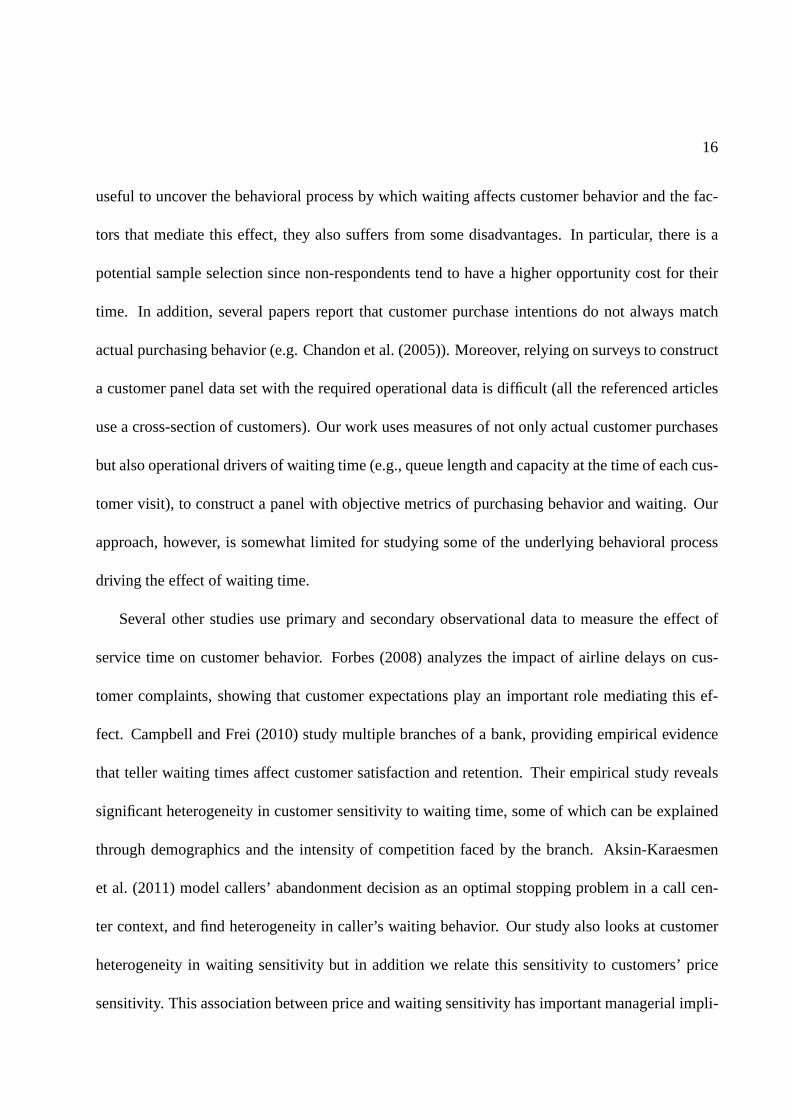
useful to uncover the behavioral process by which waiting affects customer behavior and the fac-

tors that mediate this effect, they also suffers from some disadvantages. In particular, there is a

potential sample selection since non-respondents tend to have a higher opportunity cost for their

time. In addition, several papers report that customer purchase intentions do not always match

actual purchasing behavior (e.g. Chandon et al. (2005)). Moreover, relying on surveys to construct

a customer panel data set with the required operational datais difficult (all the referenced articles

use a cross-section of customers). Our work uses measures ofnot only actual customer purchases

but also operational drivers of waiting time (e.g., queue length and capacity at the time of each cus-

tomer visit), to construct a panel with objective metrics ofpurchasing behavior and waiting. Our

approach, however, is somewhat limited for studying some ofthe underlying behavioral process

driving the effect of waiting time.

Several other studies use primary and secondary observational data to measure the effect of

service time on customer behavior. Forbes (2008) analyzes the impact of airline delays on cus-

tomer complaints, showing that customer expectations playan important role mediating this ef-

fect. Campbell and Frei (2010) study multiple branches of a bank, providing empirical evidence

that teller waiting times affect customer satisfaction andretention. Their empirical study reveals

significant heterogeneity in customer sensitivity to waiting time, some of which can be explained

through demographics and the intensity of competition faced by the branch. Aksin-Karaesmen

et al. (2011) model callers’ abandonment decision as an optimal stopping problem in a call cen-

ter context, and find heterogeneity in caller’s waiting behavior. Our study also looks at customer

heterogeneity in waiting sensitivity but in addition we relate this sensitivity to customers’ price

sensitivity. This association between price and waiting sensitivity has important managerial impli-

17

cations; for example, Afeche and Mendelson (2004) and Afanasyev and Mendelson (2010) show

that it plays an important role for setting priorities in queue and it affects the level of competition

among service providers. Section 2.5 discusses other managerial implications of this price/waiting

sensitivity relationship in the context of category pricing.

Our study uses discrete choice models based on random utility maximization to measure sub-

stitution effects driven by waiting. The same approach was used by Allon et al. (2011), who

incorporate waiting time factors into customers’ utility using a multinomial logit (MNL) model.

We instead use a random coefficient MNL, which incorporates heterogeneity and allows for more

flexible substitution patterns (Train (2003)). The random coefficient MNL model has also been

used in the transportation literature to incorporate the value of time in consumer choice (e.g. Hess

et al. (2005)).

Finally, all of the studies mentioned so far focus on settings where waiting time and congestion

generate disutility to customers. However, there is theorysuggesting that longer queues could

create value to a customer. For example, if a customers’ utility for a good depends on the number of

customers that consume it (as with positive network externalities), then longer queues could attract

more customers. Another example is given by herding effects, which may arise when customers

have asymmetric information about the quality of a product.In such a setting, longer queues

provide a signal of higher value to uninformed customers, making them more likely to join the

queue (see Debo and Veeraraghavan (2009) for several examples).

18

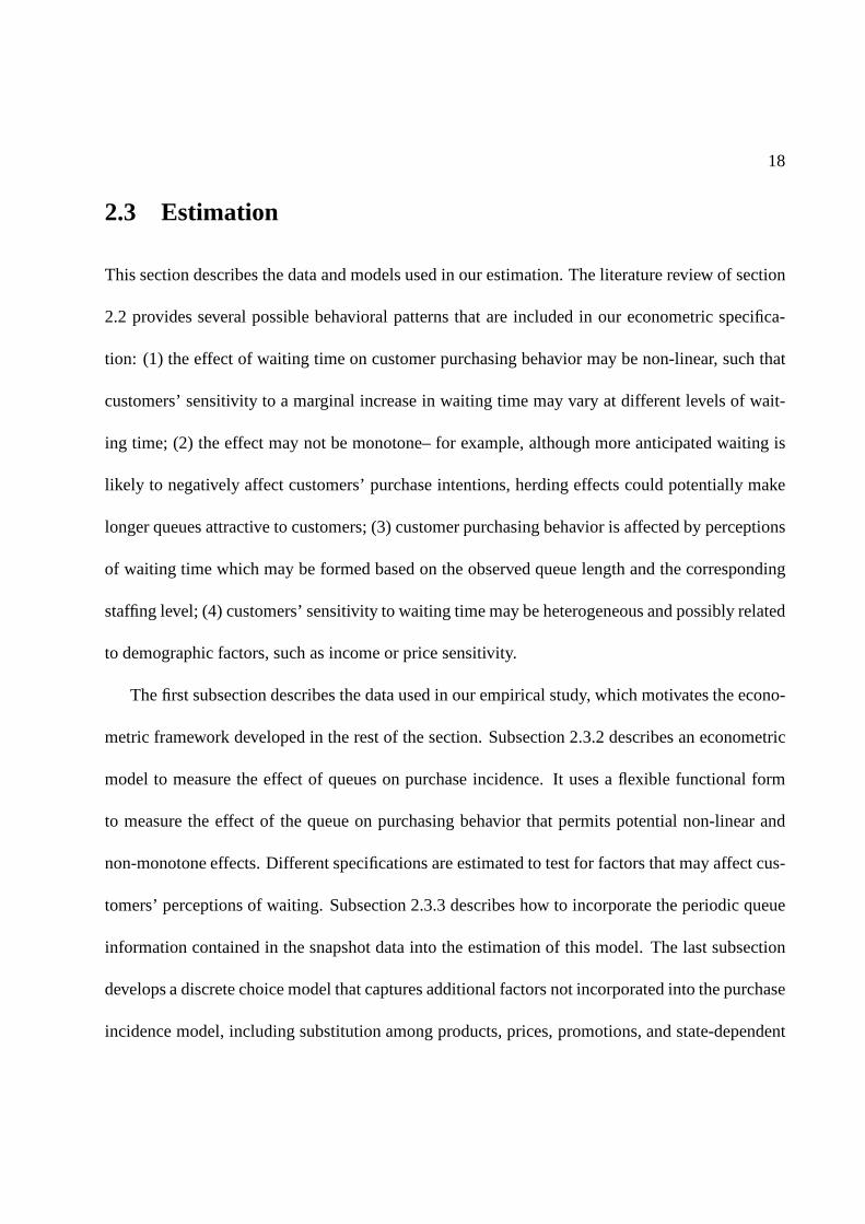
2.3 Estimation

This section describes the data and models used in our estimation. The literature review of section

2.2 provides several possible behavioral patterns that areincluded in our econometric specifica-

tion: (1) the effect of waiting time on customer purchasing behavior may be non-linear, such that

customers’ sensitivity to a marginal increase in waiting time may vary at different levels of wait-

ing time; (2) the effect may not be monotone– for example, although more anticipated waiting is

likely to negatively affect customers’ purchase intentions, herding effects could potentially make

longer queues attractive to customers; (3) customer purchasing behavior is affected by perceptions

of waiting time which may be formed based on the observed queue length and the corresponding

staffing level; (4) customers’ sensitivity to waiting time may be heterogeneous and possibly related

to demographic factors, such as income or price sensitivity.

The first subsection describes the data used in our empiricalstudy, which motivates the econo-

metric framework developed in the rest of the section. Subsection 2.3.2 describes an econometric

model to measure the effect of queues on purchase incidence.It uses a flexible functional form

to measure the effect of the queue on purchasing behavior that permits potential non-linear and

non-monotone effects. Different specifications are estimated to test for factors that may affect cus-

tomers’ perceptions of waiting. Subsection 2.3.3 describes how to incorporate the periodic queue

information contained in the snapshot data into the estimation of this model. The last subsection

develops a discrete choice model that captures additional factors not incorporated into the purchase

incidence model, including substitution among products, prices, promotions, and state-dependent

19

variables that affect purchases (e.g., household inventory). This choice model is also used to mea-

sure heterogeneity in customer sensitivity to waiting.

2.3.1 Data

We conducted a pilot study at the deli section of a super-center located in a major metropolitan area

in Latin America. The store belongs to a leading supermarketchain in this country and is located

in a working-class neighborhood. The deli section sells about 8 product categories, most of which

are fresh cold-cuts sold by the pound.

During a pilot study running from October 2008 to May 2009 (approximately 7 months), we

used digital snapshots analyzed by image recognition technology to periodically track the number

of people waiting at the deli and the number of sales associates serving it. Snapshots were taken

periodically every 30 minutes during the open hours of the deli, from 9am to 9pm on a daily basis.

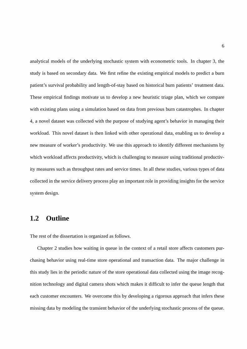
Figure 2.1 shows a sample snapshot that counts the number of customers waiting (left panel) and

the number of employees attending customers behind the delicounter (right panel).1 Throughout

the chapter, we denote the length of the deli queue at snapshot t byQt and the number of employees

serving the deli byEt.

During peak hours, the deli uses numbered tickets to implement a first-come-first-served pri-

ority in the queue. The counter displays a visible panel intended to show the ticket number of the

last customer attended by a sales associate. This information would be relevant for the purpose

of our study to complement the data collected through the snapshots; for example, Campbell and

1The numbers of customers and employees were counted by an image recognition algorithm, which achieved 98%accuracy.

20

Figure 2.1: Example of a deli snapshot showing the number of customers waiting (left) and thenumber of employees attending (right).

Frei (2010) use ticket-queue data to estimate customer waiting time. However, in our case the

ticket information was not stored in the POS database of the retailer and we learned from other

supermarkets that this information is rarely recorded. Nevertheless, the methods proposed in this

study could also be used with periodic data collected via a ticket-queue, human inspection or other

data collection procedures.

In addition to the queue and staffing information, we also collected POS data for all transactions

involving grocery purchases from Jan 1st, 2008 until the endof the study period. In the market

area of our study, grocery purchases typically include bread and about 78% of the transactions

that include deli products also include bread. For this reason, we selected basket transactions that

included bread to obtain a sample of grocery-related shopping visits. Each transaction contains

check-out data, including a time-stamp of the check-out andthe stock-keeping units (SKUs) bought

along with unit quantities and prices (after promotions). We use the POS data prior to the pilot

study period– from January to September of 2008 – to calculate metrics employed in the estimation

of some our models (we refer to this subset of the data as thecalibrationdata).

21

Using detailed information on the list of products offered at this supermarket, each cold-cut

SKU was assigned to a product category (e.g. ham, turkey, bologna, salami, etc.). Some of these

cold-cut SKUs include prepackaged products which are not sold by the pound and therefore are

located in a different section of the store.2 For each SKU, we defined an attribute indicating

whether it was sold in the deli or pre-packaged section. About 29.5% of the transactions in our

sample include deli products, suggesting that deli products are quite popular in this supermarket.

An examination on the hourly variation of the number of transactions, queue length and num-

ber of employees reveals the following interesting patterns. In weekdays, peak traffic hours are

observed around mid-day, between 11am and 2pm, and in the evenings, between 6 and 8pm. Al-

though there is some adjustment in the number of employees attending, this adjustment is insuf-

ficient and therefore queue lengths exhibit an hour-of-day pattern similar to the one for traffic. A

similar effect is observed for weekends, although the peak hours are different. In other words,

congestion generates a positive correlation between aggregate sales and queue lengths, making

it difficult to study the causal effect of queues on traffic using aggregate POS data. In our em-

pirical study, detailedcustomer transactiondata are used instead to address this problem. More

specifically, the supermarket chain in our study operates a popular loyalty program such that more

than 60% of the transactions are matched with a loyalty card identification number, allowing us

to construct a panel of individual customer purchases. Although this sample selection limits the

generalizability of our findings, we believe this limitation is not too critical because loyalty card

customers are perceived as the most profitable customers by the store. To better control for cus-

tomer heterogeneity, we focus on grocery purchases of loyalty card customers who visit the store

2This prepackaged section can be seen to the right of customernumbered 1 in the left panel of figure 1 (top-rightcorner).

22

one or more times per month on average. This accounts for a total of 284,709 transactions from

13,103 customers. Table 2.1 provides some summary statistics describing the queue snapshots, the

POS and the loyalty card data.

# obs mean stdev min max

Periodic snapshot dataLength of the queue (Q ) weekday 3671 3.76 3.81 0 26

weekend 1465 6.42 4.90 0 27Number of employees (E) weekday 3671 2.11 1.26 0 7

weekend 1465 2.84 1.46 0 9Point-of-Sales dataPurchase incidence of deli products 284,709 22.5%Loyalty card datanumber of visits per customer 13,103 62.8 45.7 20 467

Table 2.1: Summary statistics of the snapshot data, point-of-sales data and loyalty card data.

2.3.2 Purchase Incidence Model

Recall that the POS and loyalty card data are used to construct a panel of observations for each

individual customer. Each customer is indexed byi and each store visit byv. Let yiv = 1 if the

customer purchased a deli product in that visit, and zero otherwise. DenoteQiv and Eiv as the

number of people in queue and the number of employees, respectively, that were observed by the

customer during visitv. Throughout the chapter we refer toQiv andEiv altogether as thestate of

the queue.The objective of the purchase incidence model is to estimatehow the state of the queue

affects the probability of purchase of products sold in the deli. Note that we (the researchers) do not

observe the state of the queue directly in the data, which complicates the estimation. Our approach

is to infer the distribution of the state of queue using snapshot and transaction data and then plug

estimates ofQiv and Eiv into a purchase incidence model. This methodology is summarized in

23

section 2.3.4. In this subsection, we describe the purchaseincidence model assuming the state of

the queue estimates are given (step 1 in section 2.3.4); later, subsection 2.3.3 describes how to

handle the unobserved state of the queue.

In the purchase incidence model, the probability of a deli purchase, defined asp(Qiv, Eiv) ≡

Pr[yiv = 1|Qiv, Eiv] , is modeled as:

h(

p(Qiv, Eiv))

= f(Qiv, Eiv, βq) + βxXiv, (2.3.1)

whereh(·) is a link function,f(Qiv, Eiv, βq) is a parametric function that captures the impact of

the state of the queue,βq is a parameter-vector to be estimated, andXiv is a set of covariates that

capture other factors that affect purchase incidence (including an intercept). We use a logit link

function,h(x) = ln[x/(1 − x)], which leads to a logistic regression model that can be estimated

via maximum likelihood methods (ML). We tested alternativelink functions and found the results

to be similar.

Now we turn to the specification of the effect of the state of the queue,f(Qiv, Eiv, βq). Previous

work has documented that customer behavior is affected by perceptions of waiting which may

not be equal to the expected waiting time. Upon observing thestate of the queue(Qiv, Eiv),

the measureWiv = Qiv/Eiv (number of customers in line divided by the number of servers) is

proportional to the expected time to wait in line, and hence is an objective measure of waiting.

Throughout the chapter, we use the term expected waiting time to refer to theobjectiveaverage

waiting time faced by customers for a given state of the queue, which can be different from the

24

perceivedwaiting time they form based on the observed state of the queue. Our first specification

usesWiv to measure the effect of this objective waiting factor on customer behavior.

Note that the functionf(Wiv, βq) captures theoverall effect of expected waiting time on cus-

tomer behavior, which includes the disutility of waiting but also potential herding effects. The

disutility of waiting has a negative effect, whereas the herding effect has a positive effect. Because

both effects occur simultaneously, the estimated overall effect is the sum of both. Hence, the sign

of the estimated effect can be used to test which effect dominates. Moreover, as suggested by Lar-

son (1987), the perceived disutility from waiting may be non-linear. This implies thatf(Wiv, βq)

may not be monotone – herding effects could dominate in some regions whereas waiting disutility

could dominate in other regions. To account for this, we specify f(Wiv, βq) in a flexible manner

using piece-wise linear and quadratic functions.

We also estimate other specifications to test for alternative effects. As shown in some of the

experimental results reported in Carmon (1991), customersmay use the length of the line,Qiv,

as a visible cue to assess their waiting time, ignoring thespeedat which the queue moves. In the

setting of our pilot study, the length of the queue is highly visible, whereas determining the number

of employees attending is not always straightforward. Hence, it is possible for a customer to balk

from the queue based on the observed length of the line, without fully accounting for the speed at

which the line moves. To test for this, we consider specifications where the effect of the state of the

queue is only a function of the queue length,f(Qiv, βq). As before, we use a flexible specification

that allows for non-linear and non-monotone effects.

The two aforementioned models look at extreme cases where the state of the queue is fully cap-

tured either by the objective expected time to wait (Wiv), or by the length of the queue (ignoring the

25

speed of service). These two extreme cases are interesting because there is prior work suggesting

each of them as the relevant driver of customer behavior. In addition,f(Qiv, Eiv, βq) could also be

specified by placing separate weights on the length of the queue (Qiv) and the capacity (Eiv); we

also consider these additional specifications in Section 2.4.

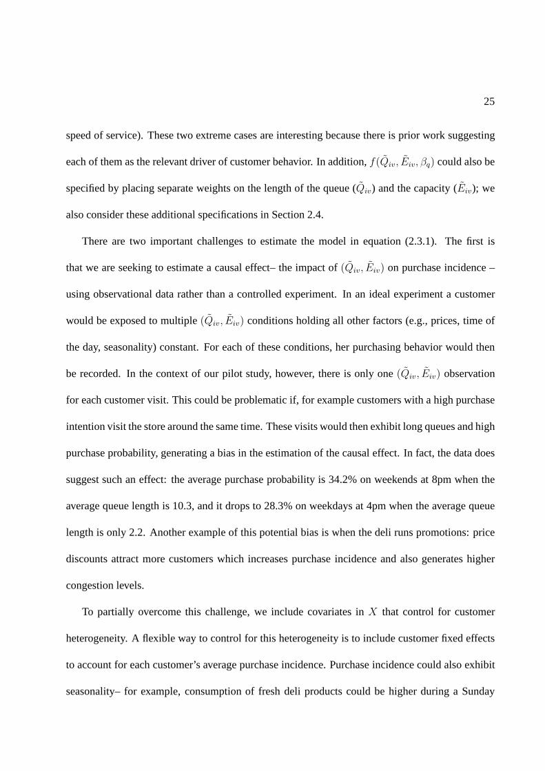
There are two important challenges to estimate the model in equation (2.3.1). The first is

that we are seeking to estimate a causal effect– the impact of(Qiv, Eiv) on purchase incidence –

using observational data rather than a controlled experiment. In an ideal experiment a customer

would be exposed to multiple(Qiv, Eiv) conditions holding all other factors (e.g., prices, time of

the day, seasonality) constant. For each of these conditions, her purchasing behavior would then

be recorded. In the context of our pilot study, however, there is only one(Qiv, Eiv) observation

for each customer visit. This could be problematic if, for example customers with a high purchase

intention visit the store around the same time. These visitswould then exhibit long queues and high

purchase probability, generating a bias in the estimation of the causal effect. In fact, the data does

suggest such an effect: the average purchase probability is34.2% on weekends at 8pm when the

average queue length is 10.3, and it drops to 28.3% on weekdays at 4pm when the average queue

length is only 2.2. Another example of this potential bias iswhen the deli runs promotions: price

discounts attract more customers which increases purchaseincidence and also generates higher

congestion levels.

To partially overcome this challenge, we include covariates in X that control for customer

heterogeneity. A flexible way to control for this heterogeneity is to include customer fixed effects

to account for each customer’s average purchase incidence.Purchase incidence could also exhibit

seasonality– for example, consumption of fresh deli products could be higher during a Sunday

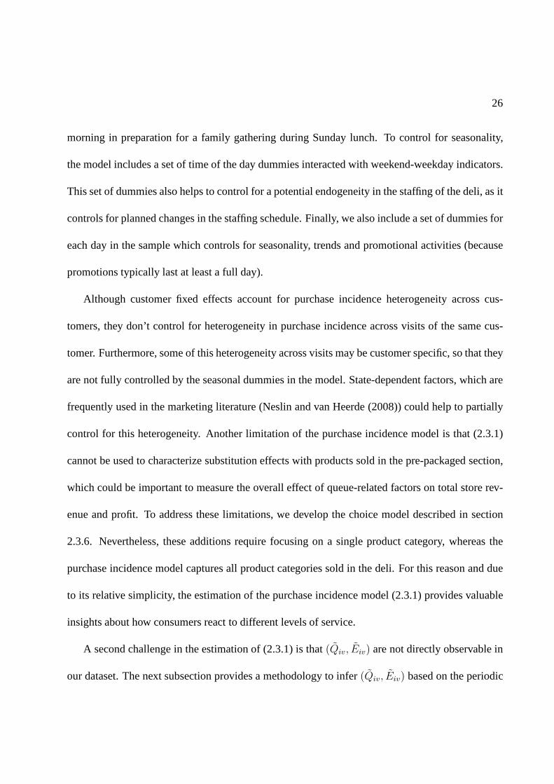
26

morning in preparation for a family gathering during Sundaylunch. To control for seasonality,

the model includes a set of time of the day dummies interactedwith weekend-weekday indicators.

This set of dummies also helps to control for a potential endogeneity in the staffing of the deli, as it

controls for planned changes in the staffing schedule. Finally, we also include a set of dummies for

each day in the sample which controls for seasonality, trends and promotional activities (because

promotions typically last at least a full day).

Although customer fixed effects account for purchase incidence heterogeneity across cus-

tomers, they don’t control for heterogeneity in purchase incidence across visits of the same cus-

tomer. Furthermore, some of this heterogeneity across visits may be customer specific, so that they

are not fully controlled by the seasonal dummies in the model. State-dependent factors, which are

frequently used in the marketing literature (Neslin and vanHeerde (2008)) could help to partially

control for this heterogeneity. Another limitation of the purchase incidence model is that (2.3.1)

cannot be used to characterize substitution effects with products sold in the pre-packaged section,

which could be important to measure the overall effect of queue-related factors on total store rev-

enue and profit. To address these limitations, we develop thechoice model described in section

2.3.6. Nevertheless, these additions require focusing on asingle product category, whereas the

purchase incidence model captures all product categories sold in the deli. For this reason and due

to its relative simplicity, the estimation of the purchase incidence model (2.3.1) provides valuable

insights about how consumers react to different levels of service.

A second challenge in the estimation of (2.3.1) is that(Qiv, Eiv) are not directly observable in

our dataset. The next subsection provides a methodology to infer (Qiv, Eiv) based on the periodic

27

data captured by the snapshots(Qt, Et) and describes how to incorporate these inferences into the

estimation procedure.

2.3.3 Inferring Queues From Periodic Data

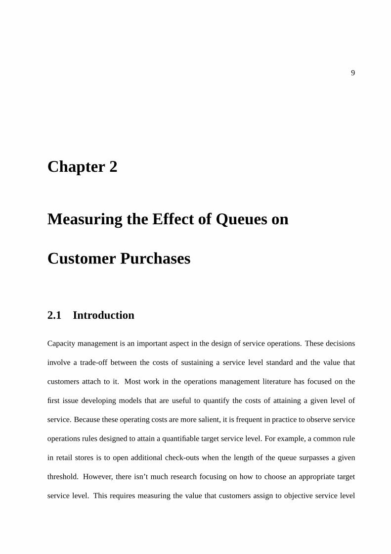
We start by defining some notation regarding event times, as summarized in Figure 2.2. Timets

denotes the observed checkout time-stamp of the customer transaction. Timeτ < ts is the time

at which the customer observed the deli queue and made her decision on whether to join the line

(whereas in reality customers could revisit the deli duringthe same visit hoping to see a shorter line,

we assume a single deli visit to keep the econometric model tractable; see footnote 9 for further

discussion). The snapshot data of the queue were collected periodically, generating time intervals

[t− 1, t), [t, t+ 1), etc. For example, if the checkout timets falls in the interval[t, t+ 1), τ could

fall in the intervals[t − 1, t), [t, t + 1), or in any other interval beforets (but not after). LetB(τ)

andA(τ) denote the index of the snapshots just before and after timeτ . In our application,τ is not

observed and we model it as a random variable , and denoteF (τ |ts) its conditional distribution

given the checkout timets.3

Figure 2.2: Sequence of events related to a customer purchase transaction.

In addition, the state of the queue is only observed at pre-specified time epochs, so even if the

deli visit timeτ was known, the state of the queue is still not known exactly. It is then necessary

3Note that in applications where the time of joining the queueis observed– for example, as provided by a tickettime stamp in a ticket-queue – it may still be unobserved for customers that decided not to join the queue. In thosecases,τ may also be modeled as a random variable for customers that did not join the queue.

28

to estimate(Qτ , Eτ ) for any givenτ based on the observed snapshot data(Qt, Et). The snapshot

data reveals that the number of employees in the system,Et, is more stable: for about 60% of the

snapshots, consecutive observations ofEt are identical. When they change, it is typically by one

unit (81% of the samples).4 WhenEt−1 = Et = c, it seems reasonable to assume that the number

of employees remained to bec in the interval[t − 1, t). When changes between two consecutive

snapshotsEt−1 andEt are observed, we assume (for simplicity) that the number of employees is

equal toEt−1 throughout the interval[t− 1, t).

Assumption 2.3.1.In any interval[t− 1, t), the number of servers in the queuing system is equal

toEt−1.

A natural approach to estimateQτ would be to take a weighted average of the snapshots around

time τ : for example, an average ofQB(τ) andQA(τ). However, this naive approach may generate

biased estimates as we will show in subsection 2.3.5. In whatfollows, we show a formal approach

to use the snapshot data in the vicinity ofτ to get a point-estimate ofQτ . Our methodology requires

the following additional assumption about the evolution ofthe queuing system:

Assumption 2.3.2. In any snapshot interval[t, t + 1), arrivals follow a Poisson process with

an effective arrival rateλt(Q,E) (after accounting for balking) that may depend on the number

of customers in queue and the number of servers. The service times of each server follow an

exponential distribution with similar rate but independent across servers.

Assumptions (2.3.1) and (2.3.2) together imply that in any interval between two snapshots the

queuing system behaves like an Erlang queue model (also known as M/M/c) with balking rate that

4However, there is still sufficient variance ofEt to estimate the effect of this variable with precision; a regressionof Et on dummies for day and hour of the day has anR2 equal to 0.44.

29

depends on the state of queue. The Markovian property implies that the conditional distribution

of Qτ given the snapshot data only depends on the most recent queueobservation before timeτ ,

QB(τ), which simplifies the estimation. We now provide some empirical evidence to validate these

assumptions.

Given that the snapshot intervals are relatively short (30 minutes), stationary Poisson arrivals

within each time interval seem a reasonable assumption. To corroborate this, we analyzed the num-

ber of cashier transactions on every half-hour interval by comparing the fit of a Poisson regression

model with a Negative Binomial (NB) regression. The NB modelis a mixture model that nests the

Poisson model but is more flexible, allowing for over-dispersion – that is, a variance larger than

the mean. This analysis suggests that there is a small over-dispersion in the arrival counts, so that

the Poisson model provides a reasonable fit to the data.5

The effective arrival rate during each time periodλt(Q,E) is modeled asλt(Q,E) = Λt ·

p(Q,E), whereΛt is the overall store traffic that captures seasonality and variations across times

of the day;p(Q,E) is the purchase incidence probability defined in (2.3.1). ToestimateΛt, we

first group the time intervals into different days of the weekand hours of the day and calculate the

average number of total transactions in each group, including those without deli purchases (see step

0 (a) in section 2.3.4). For example, we calculate the average number of customer arrivals across

all time periods corresponding to “Mondays between 9-11am”and use this as an estimate ofΛt

for those periods. The purchase probability functionp(Q,E) is also unknown; in fact, it is exactly

what the purchase incidence model (2.3.1) seeks to estimate. To make the estimation feasible, we

5The NB model assumes Poisson arrivals arrivals with a rateλ that is drawn from a Gamma distribution. Thevariance ofλ is a parameter estimated from the data; when this variance isclose to zero, the NB model is equivalentto a Poisson process. The estimates of the NB model imply a coefficient of variation forλ equal to 17%, which isrelatively low.

30

use an initial rough estimate ofp(Q,E) by estimating model (2.3.1) replacingEτ byEB(ts)−1 and

Qτ byQB(ts)−1 (step 0 (b) in section 2.3.4). We later show how this estimateis refined iteratively.

Provided an estimate ofλt(Q,E) (step 2 (a) in section 2.3.4), the only unknown primitive of

the Erlang model is the service rateµt, or alternatively, the queue intensity levelρt =maxQ[λt(Q,E)]

Et·µt.

Neitherµt nor ρt are observed, and have to be estimated from the data. To estimateρt and also

to further validate assumption 2.3.2, we compared the distribution of the observed samples ofQt

in the snapshot data with the stationary distribution predicted by the Erlang model. To do this,

we first group the time intervals intobucketsCkKk=1, such that intervals in the same bucketk

have the same number of serversEk (see step 0(c) in section 2.3.4). For example, one of these

buckets corresponds to “Mondays between 9-11am, with 2 servers”. Using the snapshots on each

time bucket we can compute the observed empirical distribution of the queue. The idea is then to

estimate a utilization levelρk for each bucket so that the predicted stationary distribution implied

by the Erlang model best matches the empirical queue distribution (step 2(b) in section 2.3.4). In

our analysis, we estimatedρk by minimizing theL2 distance between the empirical distribution of

the queue length and the predicted Erlang distribution.

Overall, the Erlang model provides a good fit for most of the buckets: a chi-square goodness

of fit test rejects the Erlang model only in 4 out of 61 buckets (at a 5% confidence level). By

adjusting the utilization parameterρ, the Erlang model is able to capture shifts and changes in the

shape of the empirical distribution across different buckets. The implied estimates of the service

rate suggest an average service time of 1.31 minutes, and thevariation across hours and days of the

week is relatively small (the coefficient of variation of theaverage service time is around 0.18).6

6We find that this service rate has a negative correlation (-0.46) with the average queue length, suggesting that

31

Now we discuss how the estimate ofQiv is refined (step 3 in section 2.3.4). The Markovian

property (given by assumptions 2.3.1 and 2.3.2) implies that the distribution ofQτ conditional on

a prior snapshot taken at timet < τ is independent of all other snapshots taken prior tot. Given

the primitives of the Erlang model, we can use the transient behavior of the queue to estimate the

distribution ofQτ . The length of the queue can be modeled as a birth-death process in continuous-

time, with transition rates determined by the primitivesEt, λt(Q,E) andρt. Note that we already

showed how to estimate these primitives. The transition rate matrix during time interval[t, t + 1),

denotedRt, is given by:[Rt]i,i+1 = λt(i, Et), [Rt]i,i−1 = mini, Et · µt, [Rt]i,i = −Σj 6=i[Rt]i,j

and zero for the rest of the entries.

The transition rate matrixRt can be used to calculate the transition probability matrix for any

elapsed times, denotedPt(s).7 For any deli visit timeτ , the distribution ofQτ conditional on any

previous snapshotQt(t < τ ) can be calculated asPr(Qτ = k|Qt) = [Pt(τ − t)]Qtk for all k ≥ 0. 8

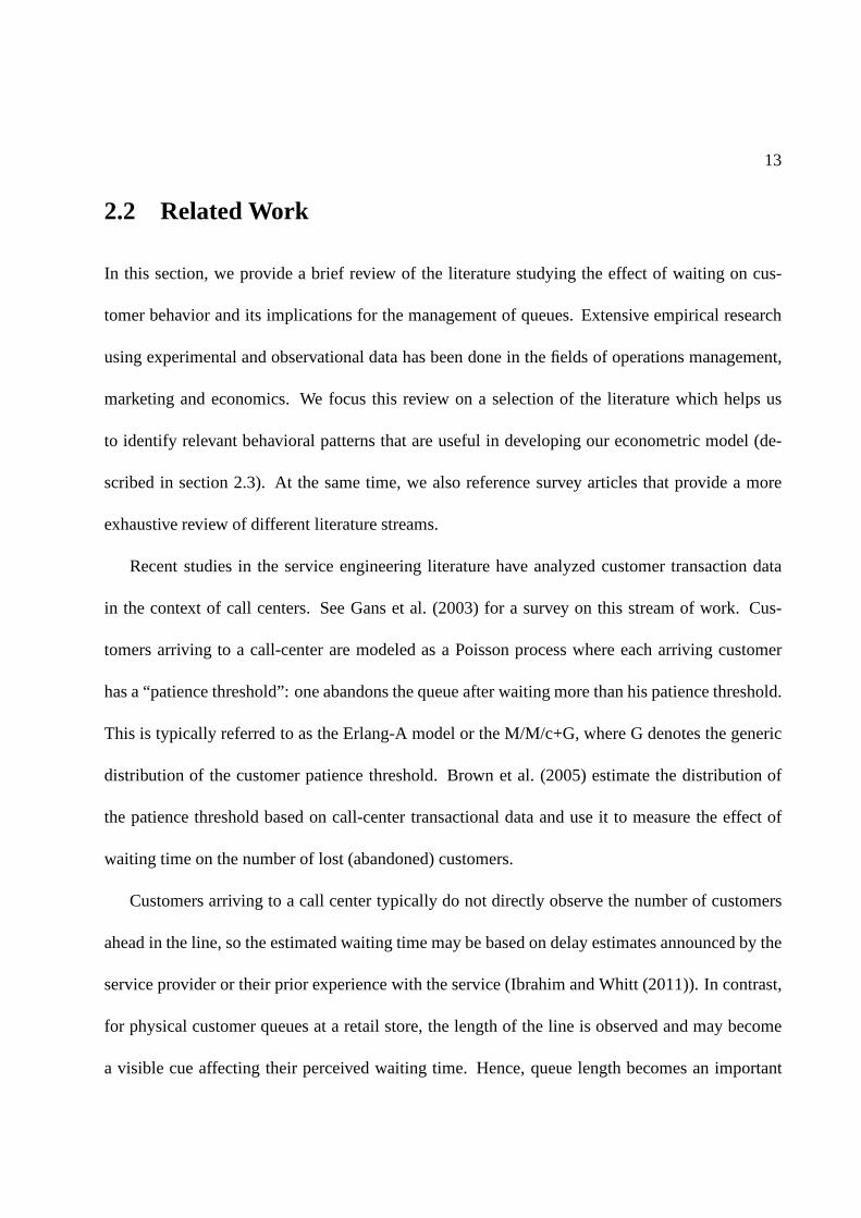
Figure 2.3 illustrates some estimates of the distribution of Qτ for different values ofτ (for

display purposes, the figure shows a continuous distribution but in practice it is a discrete distribu-

tion). In this example, the snapshot information indicatesthatQt = 2, the arrival rate isΛt = 1.2

arrivals/minute and the utilization rate isρ = 80%. Forτ = 5 minutes after the first snapshot, the

distribution is concentrated aroundQt = 2, whereas forτ = 25 minutes after, the distribution is

flatter and is closer to the steady state queue distribution.The proposed methodology provides a

servers speed up when the queue is longer (Kc and Terwiesch (2009) found a similar effect in the context of a healthcaredelivery service).

7Using the Kolmogorov forward equations, one can show thatPt(s) = eRts. See Kulkarni (1995) for furtherdetails on obtaining a transition matrix from a transition rate matrix.

8It is tempting to also use the snapshot afterτ , A(τ), to estimate the distribution ofQτ . Note, however, thatQA(τ) depends on whether the customer joined the queue or not, and is therefore endogenous. Simulation studies insubsection 2.3.5 show that usingQA(τ) in the estimation ofQτ can lead to biased estimates.

32

rigorous approach, based on queuing theory and the periodicsnapshot information, to estimate the

distribution of the unobserved dataQτ at any point in time.

Figure 2.3: Estimates of the distribution of the queue length observed by a customer for differentdeli visit times (τ ). The previous snapshot is att = 0 and shows 2 customers in queue.

In our application whereτ is not observed, it is necessary to integrate over all possible values of

τ to obtain the posterior distribution ofQiv, so thatPr(Qiv = k|tsiv) =∫

τPr(Qτ = k)dF (τ |tsiv),

wheretsiv is the observed checkout time of the customer transaction. Therefore, given a distribu-

tion for τ , F (τ |tsiv), we can compute the distribution ofQiv, which can then be used in equation

(2.3.1) for model estimation. In particular, the unobserved valueQiv can be replaced by the point

estimate that minimizes the mean square prediction error, i.e., its expected valueE[Qiv] (step 3(b)

in section 2.3.4).9

In our application, we discretize the support ofτ so that each 30-minutes snapshot interval

9Although formally the model assumes a single visit to the deli, the estimation is actually using a weighted averageof many possible visit times to the deli. This makes the estimation more robust if in reality customers re-visit thequeue more than once in the hope of facing a shorter queue.

33

is divided into a grid of one-minute increments and calculate the queue distribution accordingly.

However, since we do not have precise data to determine the distribution of the elapsed time be-

tween a deli visit and the cashier time-stamp, an indirect method (described in appendix A.1) is

used to estimate this distribution based on estimates of theduration of store visits and the location

of the deli within the supermarket. Based on this analysis, we determined that a uniform in range

[0,30] minutes prior to check-out time is a reasonable distribution for τ .

Assumption 2.3.3.Customers visit the deli once, and this visiting time is uniformly distributed

with range [0,30] minutes before check-out time.

To avoid problems of endogeneity, we determine the distribution of Qiv conditioning on a

snapshot that is at least 30 minutes before checkout time (that is, the second snapshot before

checkout time) to ensure that we are using a snapshot that occurs before the deli visit time.

Finally, steps 1-3 in section 2.3.4 are run iteratively to refine the estimates of effective arrival

rateλt(Q,E), the system intensityρk, and the queue lengthQiv. In our application, we find that

the estimates converge quickly after 3 iterations.10

2.3.4 Outline of the Estimation Procedure

The outline of the estimation procedure is summarized below.

• Step 0.Initialize the estimation.

1. Calculate the average store trafficΛt using all cashier transactions (including those

10As a convergence criteria, we used a relative difference of 0.1% or less between two successive steps.

34

without deli purchases) for different hours of the day and days of the week (e.g. week-

days between 9-11am).

2. Initialize the state of the queue(Qiv, Eiv) observed by customeri in visit v as the

second previous snapshot before check-out time.

3. Group the snapshot data intotime bucketswith observations for the same time of the

day, day of the week and the same number of employees. For example, one bucket

could contain snapshots taken on weekdays between 9-11am with 2 employees attend-

ing. For each time bucket, compute the empirical distribution of the queue length based

on the snapshot data.

• Step 1.Estimate purchase incidence model 2.3.1 via ML assuming state of queue(Qiv, Eiv)

is observed.

• Step 2.Estimate the queue intensityρt on each time bucket.

1. Based on the estimated store trafficΛt and purchase incidence probabilityp(Q,E),

calculate the effective arrival rateλt(Q,E)=Λtp(Q,E) for each possible state of the

queue in time buckett.

2. Compute the stationary distribution of the queue length on each time buckett as a func-

tion of the queue intensityρt andλt(Q,E): for each time bucket, choose the queue

intensityρt that best matches the predicted stationary distribution tothe observed em-

pirical distribution of the length of the queue (computed inStep 0(c)).

• Step 3.Update the distribution of the observed queue lengthQiv.

35

1. Compute the transition probability matrixPt(s).

2. For a given deli visit timeτ , calculate the distribution ofQτ usingPt(s).

3. Integrate over all possible deli visit timesτ to find the distribution ofQiv. UpdateQiv

by its expectation based on this distribution.

4. Repeat fromStep 1until the estimated length of the queue,Qiv, converges.

2.3.5 Simulation Test

Our estimation procedure has several sources of missing data that need to be inferred: time at

which the customer arrives at the deli is inferred from her check-out time, and the state of the

queue observed by a customer is estimated from the snapshot data. This subsection describes

experiments using simulated data to test whether the proposed methodology can indeed recover

the underlying model parameters under assumptions 2.3.1 and 2.3.2.

The simulated data are generated as follows. First, we simulate a Markov queuing process with

a single server: customers arrive following a Poisson process and join the queue with probabil-

ity logit(f(Q)), wheref(Q) is quadratic inQ and has the same shape as we obtained from the

empirical purchase incidence model (we also considered piece-wise linear specifications and the

effectiveness of the method was similar). After visiting the queue, the customer spends some addi-

tional random time in the store (which follows a uniform [0,30] minutes) and checks out. Snapshots

are taken to record the queue length every 30 minutes. The arrival rate and traffic intensity are set

to be equal to the empirical average value.

Figure 2.4 shows a comparison of different estimation approaches. The black line, labeled

36

True Response, represents the customer’s purchase probabilities that were used to simulate the

data. A consistent estimation shouldgenerate estimates that are close to this line. Three estimation

approaches, shown with dashed lines in the figure, were compared: (i) Using the true state of

the queue,Qτ . Although this information is unknown in our data, we use it as a benchmark to

compare with the other methods. As expected, the purchase probability is estimated accurately

with this method, as shown in the black dashed line. (ii) Using the average of the neighboring

snapshots12(QB(τ) + QA(τ)) and integrating over all possible values ofτ . Although the average

of neighboring snapshots provides an intuitive estimate ofQτ , this method gives biased estimates

of the effect of the state of the queue on purchase incidence (the dots-and-dashes line). This is

becauseQA(τ), the queue length in the snapshot followingτ depends on whether the customer

purchased or not, and therefore is endogenous (if the customer joins the queue, then the queue

following her purchase is likely to be longer). The bias appears to be more pronounced when the

queue is short, producing a (biased) positive slope for small values ofQτ . (iii) Using the inference

method described in subsection 2.3.3 to estimateQτ , depicted by the dotted line; this gives an

accurate estimate of the true curve. We conducted more testsusing different specifications for the

effect of the state of the queue and the effectiveness of the estimation method was similar.

2.3.6 Choice Model

There are three important limitations of using the purchaseincidence model (2.3.1). The first is that

it doesn’t account for changes in a customer’s purchase probability over time, other than through

seasonality variables. This could be troublesome if customers plan their purchases ahead of time,

as we illustrate with the following example. A customer who does weekly shopping on Saturdays

37

0 2 4 6 8 10 12 14 16 18 20

.22

.23

0.24

0.25

0.26

0.27

0.28

0.29

0.30

0.31

Queue

purc

hase

pro

babi

lity

Estimation with Simulated Data

true responseusing actual queue length Q

τ

using average of neighboring snapshotsusing conditional mean based on previous snapshot

Figure 2.4: Estimation results of the purchase incidence model using simulated data.

and is planning to buy ham at the deli section visits the storeearly in the morning when the deli

is less crowded. This customer visits the store again on Sunday to make a few “fill-in” purchases

at a busy time for the deli and does not buy any ham products at the deli because she purchased

ham products the day before. In the purchase incidence model, controls are indeed included to

capture theaveragepurchase probability at the deli for this customer. However, these controls

don’t capture thechangesto this purchase probability between the Saturday and Sunday visits.

Therefore, the model would mistakenly attribute the lower purchase incidence on the Sunday visit

to the higher congestion at the deli whereas in reality the customer would not have purchased

regardless of the level of congestion at the deli on that visit.

A second limitation of the purchase incidence model (2.3.1)is that it cannot be used to attach

an economic value to the disutility of waiting by customers.One possible approach would be

38

to calculate an equivalent price reduction that would compensate the disutility generated by a

marginal increase in waiting. Model (2.3.1) cannot be used for this purpose because it does not

provide a measure of price sensitivity. A third limitation is that model (2.3.1) does not explicitly

capture substitution with products that do not require waiting (e.g., the pre-packaged section),

which can be useful to quantify the overall impact of waitingon store revenues and profit.

To overcome these limitations, we use a random utility model(RUM) to explain customer

choice. As it is common in this type of models, the utility of acustomeri for productj during

a visit v, denotedUijv, is modeled as a function of product attributes and parameters that we

seek to estimate. Researchers in marketing and economics have estimated RUM specifications

using scanner data from a single product category (e.g., Guadagni and Little (1983) model choices

of ground coffee products; Bucklin and Lattin (1991) model saltine crackers purchases; Fader

and Hardie (1996) model fabric softener choices; Rossi et al. (1996) model choices among tuna

products). Note that although deli purchases include multiple product categories, using a RUM to

model customer choice requires us to select a single productcategory for which purchase decisions

are independent from choices in other categories and where customers typically choose to purchase

at most one SKU in the category. The ham category appears to meet these criteria. The correlations

between purchases of ham and other cold-cut categories are relatively small (all less than 8% in

magnitude). About 93% of the transactions with ham purchases included only one ham SKU. In

addition, it is the most popular category among cold-cuts, accounting for more than 33% of the

total sales. The ham category has 75 SKUs, 38 of which are soldin the deli and the rest in the pre-

packaged section, and about 85% of ham sales are generated inthe deli section. In what follows,

39

we describe a RUM framework to model choices among products in the ham category. Table 2.2

shows statistics for a selection of products in the ham category.

Product Avg Price St.Dev. Price Share

1 0.67 0.10 21.23%2 0.40 0.04 9.37%3 0.53 0.06 7.12%4 0.59 0.06 6.13%5 0.64 0.07 5.66%6 0.24 0.01 5.49%7 0.52 0.07 3.97%8 0.54 0.07 3.10%9 0.56 0.07 2.85%10 0.54 0.08 2.20%

Table 2.2: Statistics for the ten most popular ham products,as measured by the percent of transac-tions in the category accounted by the product (Share). Prices are measured in local currency perkilogram (1 unit of local currency = US$21, approximately).

One advantage of using a RUM to characterize choices among SKUs in a category is that it

allows us to include product specific factors that affect substitution patterns. Although many of the

product characteristics do not change over time and can be controlled by a SKU specific dummy,

our data reveals that prices do fluctuate over time and could be an important driver of substitution

patterns. Accordingly, we incorporate product-specific dummies,αj , and product prices for each

customer visit (PRICEvj) as factors influencing customers’ utility for productj. Including prices

in the model also allows us to estimate customer price sensitivity, which we use to put a dollar tag

on the cost of waiting.

As in the purchase incidence model (2.3.1), it is important to control for customer heterogene-

ity. Due to the size of the data set, it is computationally challenging to estimate a choice model

including fixed effects for each customer. Instead, we control for each customer’s average buying

40

propensity by including a covariate measuring the average consumption rate of that customer, de-

noted CRi. This consumption rate was estimated using calibration data as done by Bell and Lattin

(1998). We also use the methods developed by these authors toestimate customers’ inventory of

ham products at the time of purchase, based on a customers’ prior purchases and their consumption

rate of ham products. This measure is constructed at the category level and is denoted by INViv.

We use the following notation to specify the RUM. LetJ be the set of products in the product

category of interest (i.e., ham).JW is the set of products that are sold at the deli section and,

therefore, potentially require the customer to wait.JNW = J\JW is the set of products sold in

the pre-packaged section which require no waiting. LetTv be a vector of covariates that capture

seasonal sales patterns, such as holidays and time trends. Also let1[·] denote the indicator function.

Using these definitions, customeri’s utility for purchasing productj during store visitv is specified

as follows:

Uijv = αj + 1[j ∈ JW ]βqi f

(

Qiv, Eiv

)

+ 1[j ∈ JW ]βfreshi

+βpricei PRICEjv + γcrCRi + γinvINV iv + γTTv + εijv, (2.3.2)

whereεijv is an error term capturing idiosyncratic preferences of thecustomer andf(

Qiv, Eiv

)

captures the effect of the state of the queue on customers’ preference. Note that the indicator

function1[j ∈ JW ] adds the effect of the queue only to the utility of those products which are

sold at the deli section (i.e.,j ∈ JW ) and not to products that do not require waiting. As in the

purchase incidence model (2.3.1), the state of the queue(Qiv, Eiv) is not perfectly observed but the

41

method developed in subsection 2.3.3 can be used to replace these by point-estimates.11 An outside

good, denoted byj = 0, accounts for the option of not purchasing ham, with utilitynormalized to

Ui0v = εi0v. The inclusion of an outside good in the model enables us to estimate how changes in

waiting time affect the total sales of products in this category (i.e., category sales).

Assuming a standard extreme value distribution forεijv, the RUM described by equation (2.3.2)

becomes a random-coefficients multinomial logit. Specifically, the model includes consumer-

specific coefficients forPrice (βpricei ), the dummy variable for products sold in the deli (βfresh

i ),

as opposed to products sold in the pre-package section) and for some of the coefficients associated

with the effect of the queue (βqi ). These random coefficients are assumed to follow a Multivariate

Normal distribution with meanθ = (θprice, θfresh, θq)′ and covariance matrixΩ, which we seek

to estimate from the data. Including random-coefficients for Price andFresh is useful to accom-

modate more flexible substitution patterns based on these characteristics, overcoming some of the

limitations imposed by the independence of irrelevant alternatives of standard multinomial logit

models. For example, if customers are more likely to switch between products with similar prices

or between products that are sold in the deli (or alternatively, in the pre-packaged section), then the

inclusion of these random coefficients will enable us to model that behavior. In addition, allow-

ing for covariation betweenβpricei , βfresh

i andβqi provides useful information on how customers’

sensitivity to the state of the queue relates to the sensitivity to the other two characteristics.

The estimation of the model parameters is implemented usingstandard Bayesian methods (see

Rossi and Allenby (2003)). The goal is to estimate: (i) the SKU dummiesαj; (ii) the effect of the

11In our empirical analysis, we also performed a robustness check where instead of replacing the unobserved queuelengthQiv by point estimates, we sample different queue lengths from the estimated distribution ofQiv. The resultsobtained with the two approaches are similar.

42

consumption rate (γcr), inventory (γinv), and seasonality controls (γT ) on consumer utility; and

(iii) the distribution of the price and queue sensitivity parameters, which is governed byθ andΩ.

In order to implement this estimation, we define prior distributions on each of these parameters of

interest:αj ∼ N(α, σα), γ ∼ N(γ, σγ), θ ∼ N(θ, σθ) andΩ ∼ Inverse Wishart(df, Scale). For

estimation, we specify the following parameter values for these prior distributions:α = γ = θ = 0,

σα = σγ = σθ = 100, df=3 and Scale equal to the identity matrix. These choices produce weak

priors for parameter estimation. Finally, the estimation is carried out using Markov chain Monte

Carlo (MCMC) methods. In particular, each parameter is sampled from its posterior distribution

conditioning on the data and all other parameter values (Gibbs sampling). When there is no closed

form expression for these full-conditional distributions, we employ Metropolis Hastings methods

(see Rossi and Allenby (2003)). The outcome of this estimation process is a sample of values from

the posterior distribution of each parameter. Using these values, a researcher can estimate any

relevant statistic of the posterior distribution, such as the posterior mean, variance and quantiles of

each parameter.

2.4 Empirical Results

This section reports the estimates of the purchase incidence model (2.3.1) and the choice model

(2.3.2) using the methodology described in subsection 2.3.3 to impute the unobserved state of the

queue.

43

2.4.1 Purchase Incidence Model Results

Table 2.3 reports a summary of alternative specifications ofthe purchase incidence model (2.3.1).

All the specifications include customer fixed effects (11,487 of them), daily dummies (192 of

them), and hour of the day dummies interacted with weekend/holiday dummies (30 of them). A

likelihood ratio (LR) test indicates that the daily dummiesand hour of the day interacted with

weekend/holiday dummies are jointly significant (p value< 0.0001), and so are the customer fixed

effects (p value< 0.0001).

Model Form Metric dim(βq) log-likelihood AIC rank BIC rank

I Linear W 1 -118195.3 259808.6 5 382023.4 3II Quadratic W 2 -118193.1 259806.2 4 382031.5 4III Piecewise W 4 -118192.8 259809.7 6 382055.8 6IV Linear Q 1 -118189.5 259797.0 3 382011.8 1V Quadratic Q 2 -118185.4 259790.8 1 382016.0 2VI Piecewise Q 4 -118184.9 259793.7 2 382039.8 5

Table 2.3: Goodness of fit results on alternative specifications of the purchase incidence model(equation (2.3.1)).

Different specifications of the state of the queue effect areare compared, which differ in terms

of: (1) the functional form for the queuing effectf(Q, E, βq), including linear, piecewise linear and

quadratic polynomial; and (2) the measure capturing the effect of the state of the queue, including:

(i) expected time to wait,W = Q/E; and (ii) the queue length,Q (we omit the tilde in the table). In

particular, models I-III are linear, quadratic, and piecewise linear (with segments at(0, 5, 10, 15))

functions ofW ; model IV-VI are the corresponding models ofQ. We discuss other models later

in this section. The table reports the number of parameters associated with the queuing effects

(dim(βq)), the log-likelihood achieved in the MLE, and two additional measures of goodness of fit,

44

Akaike Information Criterion (AIC) and Bayesian Information Criterion (BIC), that are used for

model selection.

Using AIC and BIC to rank the models, the specifications withQ as explanatory variables

(models IV-VI) all fit significantly better than the corresponding ones withW (models I-III), sug-

gesting that purchase incidence appears to be affected moreby the length of the queue rather than

the speed of the service. A comparison of the estimates of themodels based onQ is shown in table

2.4 and figure 2.5 (which plots the results of model IV-VI). Considering models V and VI, which

allow for a non-linear effect ofQ, the pattern obtained in both models is similar: customers appear

to be insensitive to the queue length when it is short, but they balk when experiencing long lines.

This impact on purchase incidence can become quite large forqueue lengths of 10 customers and

more. In fact, our estimation indicates that increasing thequeue length from 10 to 15 customers

would reduce purchase incidence from 30% to 27%, corresponding to a 10% drop in sales.

Variable Coef. Std. Err. z

Model IV Q -0.0133 0.0024 -5.46Model V Q− 5.7 -0.00646 0.00340 -1.90

(Q− 5.7)2 -0.00166 0.00066 -2.50Model VI Q0−5 0.0056 0.0079 0.71

Q5−10 -0.0106 0.0042 -3.54Q10−15 -0.0199 0.0068 -2.92Q15+ -0.0303 0.0210 -1.44

Table 2.4: MLE results for purchase incidence model (equation (2.3.1))

The AIC scores in Table 2.3 also suggest that the more flexiblemodels V and VI tend to provide

a better fit than the less flexible linear model IV. The BIC score, which puts a higher penalization for

the additional parameters, tends to favor the more parsimonious quadratic models V and the linear

model IV. Considering both the AIC and BIC score, we concludethat the quadratic specification

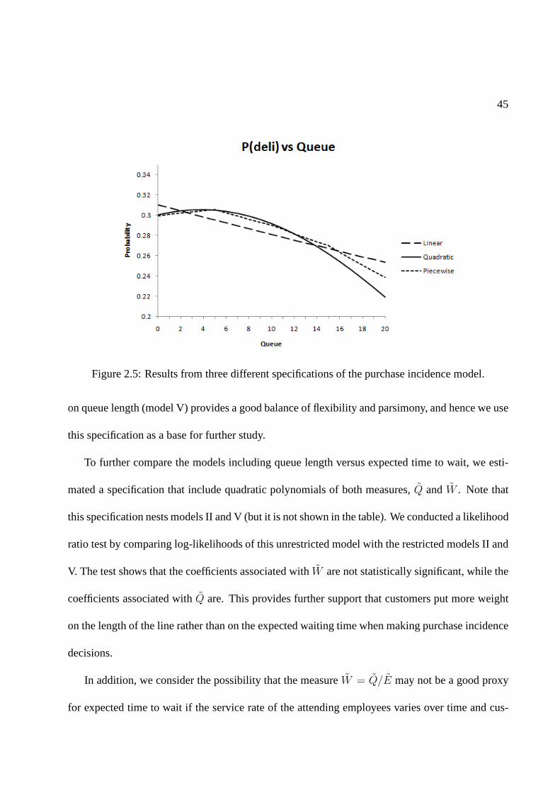
45

Figure 2.5: Results from three different specifications of the purchase incidence model.

on queue length (model V) provides a good balance of flexibility and parsimony, and hence we use

this specification as a base for further study.

To further compare the models including queue length versusexpected time to wait, we esti-

mated a specification that include quadratic polynomials ofboth measures,Q andW . Note that

this specification nests models II and V (but it is not shown inthe table). We conducted a likelihood

ratio test by comparing log-likelihoods of this unrestricted model with the restricted models II and

V. The test shows that the coefficients associated withW are not statistically significant, while the

coefficients associated withQ are. This provides further support that customers put more weight

on the length of the line rather than on the expected waiting time when making purchase incidence

decisions.

In addition, we consider the possibility that the measureW = Q/E may not be a good proxy

for expected time to wait if the service rate of the attendingemployees varies over time and cus-

46

tomers can anticipate these changes in the service rate. Recall, however, that our analysis in section

2.3.3 estimates separate service rates for different days and hours, and shows that there is small

variation across time. Nevertheless, we constructed an alternative proxy of expected time to wait

that accounts for changes in the service rate:W ′ = W/µ, whereµ is the estimated service rate

for the corresponding time period. ReplacingW byW ′ lead to estimates that were similar to those

reported in 2.3.

Although the expected waiting time doesn’t seem to affect customer purchase incidence as

much as the queue length, it is possible that customers do take into account the capacity at which

the system is operating– i.e., the number of employees – in addition to the length of the line. To test

this, we estimated a specification that includes both the queue lengthQ (as a quadratic polynomial)

and the number of serversE as separate covariates.12 The results suggest that the number of servers

E has a positive impact which is statistically significant, but small in magnitude (the coefficient

is 0.0201 with standard error 0.0072). Increasing staffing from 1 to 2 at the average queue length

only increases the purchase probability by 0.9%. To compare, shortening the queue length from 12

to 6 customers, which is the average length, would increase the purchase probability by 5%. Since

both scenarios halve the waiting time, this provides further evidence that customers focus more on

the queue length than the objective expected waiting time when making purchase decisions. We

also found that the effect of the queue length in this model isalmost identical to the one estimated

in Model V (which omits the number of servers). We therefore conclude that although the capacity

does seem to play a role in customer behavior, its effect is minor relative to the effect of the length

of the queue.

12We also estimated models with quadratic term forE but this additional coefficient was not significant.

47

Finally, we emphasize that the estimates provide an overalleffect of the state of the queue

on customer purchases. The estimates suggest that, for queue lengths above the mean (about 5

customers in line) the effect is significantly negative, which implies that the disutility of waiting

seems to dominate any potential herding effects of the queue, while for queue lengths below the

mean neither effect is dominant. In our context, herding effects could still be observed, for ex-

ample, if customers passing by the deli section infer from a long line that the retailer must be

offering an attractive deal, or if long lines make the deli section more salient. While the absence

of a dominant herding effect seems robust for theaveragecustomer, we further tested model V

on subsamples of frequent customers (i.e., customers that made 30 or more visits during the study

period) and infrequent customers (i.e., customers that made less than 30 visits), with the idea that

infrequent customers would be less informed and might potentially learn more from the length of

the line. However, we found no significant differences between the estimates. We also partitioned

customers into new customers and existing customers (customers are considered to be new within

the first 2 months of their first visit), with the idea that new customers should be less informed.13

Again, we found no significant differences in the estimated results for the two groups. In sum-

mary, the statistical evidence in our results are not conclusive on the presence of dominant herding

effects.13We used one year of transaction data prior to the study periodto verify the first customer visit date. We also tried

other definitions of new customers (within 3 months of the first visit), and the results were similar.

48

2.4.2 Choice Model results

In this subsection we present and discuss the results obtained for the choice model described in sec-

tion 2.3.6. The specification for the queuing effectf(Q, E) is based on the results of the purchase

incidence model. In particular, we used a quadratic function of Q, which balanced goodness-of-fit

and parsimony in the purchase incidence model. The utility specification includes product-specific

intercepts, prices, consumption rate (CR), household inventory (INV) and controls for seasonality

as explanatory variables. The model incorporates heterogeneity through random coefficients for

Price, theFreshdummy and the linear term of the length of the queue (Q). We use 2,000 randomly

selected customers in our estimation. After running 20,000MCMC iterations and discarding the

first 10,000 iterations, we obtained the results presented in Table 2.5 (the table omits the estimates

of the product-specific intercept and seasonality). The left part of the table shows the estimates of

the average effects, with the estimated standard error (s.e., measured by the standard deviation of

the posterior distribution of each parameter). The right part of the table shows the estimates of the

variance-covariance matrix (Ω) characterizing the heterogeneity of the random coefficientsβpricei ,

βfreshi andβq

i .

Average Effect Variance/Covariance (Ω)estimate s.e. estimate s.e.

Inv -0.091 0.026 Ω(Price,Price) 31.516 1.671CR 1.975 0.150 Ω(Fresh,Fresh) 7.719 0.436

Fresh 0.403 0.112 Ω(Q,Q) 0.403 0.083Price -9.692 0.203 Ω(Fresh,Q) 0.020 0.144

Q -0.058 0.061 Ω(Price,Fresh) -14.782 0.821Q2 -0.193 0.122 Ω(Price,Q) -0.508 0.267

Table 2.5: Estimation results for the choice model (equation 2.3.2). The estimate and standard error(s.e.) of each parameter correspond to the mean and standarddeviation of its posterior distribution.

49

Price, inventory, and consumption rate all have the predicted signs and are estimated precisely.

The average of the implied price elasticities of demand is -3. The average effects of the queue

coefficients imply qualitatively similar effects as those obtained in the purchase incidence model:

consumers are relatively insensitive to changes in the queue length in theQ = 0 to Q = 5 range,

and then the purchase probability starts exhibiting a sharper decrease for queue length values at or

aboveQ = 6.

These results can also be used to assign a monetary value to customers’ cost of waiting. For

example, for an average customer in the sample, an increase from 5 to 10 customers in queue is

equivalent to a 1.7% increase in price. Instead, an increasefrom 10 to 15 customers is equivalent to

a 5.5% increase in price, illustrating the strong non-linear effect of waiting on customer purchasing

behavior.

The estimates also suggest substantial heterogeneity in customers’ price sensitivities (estimates

on the right side of Table 2.5). The estimated standard deviation of the random price coefficients

is 5.614, which implies a coefficient of variation of 57.9%. There is also significant heterogeneity

in customer sensitivity to waiting, as measured by the standard deviation of the linear queue effect,

which is estimated to be 0.635. The results also show a negative relationship between price and

waiting sensitivity and between price and the fresh indicator variable.

To illustrate the implications of the model estimates in terms of customer heterogeneity, we

measured the effect of the length of the queue on three customer segments with different levels

of price sensitivity: a price coefficient equal to the mean; one standard deviation below the mean

(labeled high price sensitivity); and one standard deviation above the mean (labeled low price

sensitivity). To compute these choice probabilities, we considered customer visits with average

50

levels of prices, consumption rate and consumer inventory.Given the negative correlation between

the price random coefficient and the two other random coefficients, customers with a weaker price

sensitivity will in turn have stronger preferences for fresh products and a higher sensitivity to the

length of the queue and, hence, be more willing to wait in order to buy fresh products. Figure

2.6 illustrates this pattern, showing a stronger effect of the length of the queue in the purchase

probability of the low price sensitivity segment. Interestingly, the low price sensitivity segment is

also the most profitable, with a purchase incidence that morethan doubles that of the high price

sensitivity segment (for small values of the queue length).This has important implications for

pricing product categories under congestion effects, as wediscuss in the next section.

Figure 2.6: Purchase probability of ham products in the delisection versus queue length for threecustomer segments with different price sensitivity.

Finally, since our choice model also considers products that do not require waiting, we measure

51

the extent by which lost sales of fresh products due to a higher queue length are substituted by

sales of the pre-packaged products. In this regard, our results show that when the length of the

line increases, for example, from 5 to 10 customers, only 7% of the deli lost sales are replaced by

non-deli purchases. This small substitution effect can be explained by the large heterogeneity of

theFreshrandom coefficient together with the relatively small shareof purchases of pre-packaged

products that we observe in the data.

2.5 Managerial Implications

The results of the previous section suggest that: (1) purchase incidence appears to be affected

more by the length of the line rather than the speed of the service; and (2) there is heterogeneity

in customers’ sensitivity to the queue length, which is negatively correlated with their price sensi-

tivity. We discuss three important managerial insights implied by these findings. The first shows

that pooling multiple identical queues into a single multi-server queue may lead to an increase

in lost sales. The second considers the benefit of adding servers when making staffing decisions.

The third discusses the implications of the externalities generated by congestion for pricing and

promotion management in a product category.

2.5.1 Queuing Design

The result from the purchase incidence model that customersreact more to the length of the queue

than the speed of service has implications on queuing management policies. In particular, we are

interested in comparing policies between splitting versusmerging queues.

52

It is well known that anM/M/c pooled queuing system achieves much lower waiting time than

a system with separateM/M/1 queues at the same utilization levels. Therefore, if waiting time

is the only measure of customer service, then pooling queuesis beneficial. However, Rothkopf

and Rech (1987) provide several reasons for why pooling queues could be less desirable. For

example, there could be gains from server specialization that can be achieved in the separate queue

setting. Cachon and Zhang (2007b) look at this issue in a setting where two separate queues

compete against each other for the allocation of (exogenous) demand, and show that using a system

with separate queues is more effective (relative to a pooledsystem) at providing the servers with

incentives to increase the service rate. The results in our study provide another argument for why

splitting queues may be beneficial: although the waiting time in the pooled system is shorter, the

queue is longer and this can influence demand. If customers make their decision of joining a queue

based on its queue length, as we find in our empirical study, then a pooled system can lead to fewer

customers joining the system and therefore increase lost sales. We illustrate this in more detail

with the following example.

Consider the following queuing systems: apooledsystem given by anM/M/2 queue with

constant arrival rateλ and asplit JSQsystem with two parallel single-server queues with same

overall arrival given by a Poisson process with rateλ and where customers join the shortest queue

upon arrival and assuming that after joining a line customers don’t switch to a different line (i.e.,

no jockeying). If there is no balking– that is, all customersjoin the queue – it can be shown that

the pooled system dominates the split JSQ system in terms of waiting time. However, the queues

are longer in the pooled system, so if customers may walk awayupon arrival and this balking rate

increases with the queue length, then the pooled system may lead to fewer sales.

53

To evaluate the differences between the two systems, we numerically compute the average

waiting time and revenue for both. For the split JSQ system, the approximate model proposed by

Rao and Posner (1987) is used to numerically evaluate the system performance. When the queue

length is equal ton and the number of servers isc, the arrival rate isλPr(join|Q = n,E = c),

wherePr(join|Q = n,E = c) is customers’ purchase probability. In this numerical example,

we set the purchase probabilities based on the estimates of the purchase incidence model that

includes the quadratic specification ofQ. Traffic intensity is defined asρ = maxn λPr(join|Q =

n,E = c)/µ and revenue is defined as the number of customers that join thequeue. Figure 2.7

shows the long-run steady-state average waiting time and average revenue of the two systems. As

expected, the pooledM/M/2 system always achieves shorter waiting time. However theM/M/2

system generates less revenue as it suffers more traffic lossdue to long queues, and the difference

increases as the traffic intensity approaches one. In our particular case, the split JSQ system gains

2.7% more revenue while increasing the average waiting timeby more than 70% at the highest

level of utilization compared to the pooled system. These results imply that when moving towards

a pooled system, it may be critical to provide information about the expected waiting time so that

customers do not anchor their decision primarily on the length of the line, which tends to increase

when the system is pooled.

2.5.2 Implications for Staffing Decision

The model used in 2.5.1 also provides insights for making staffing decisions. For example, consider

a typical weekday 11:00-12:00 time window versus a weekend 11:00-12:00 window. Given the

average customer arrival rates observed at the deli, the minimum capacity needed to meet the

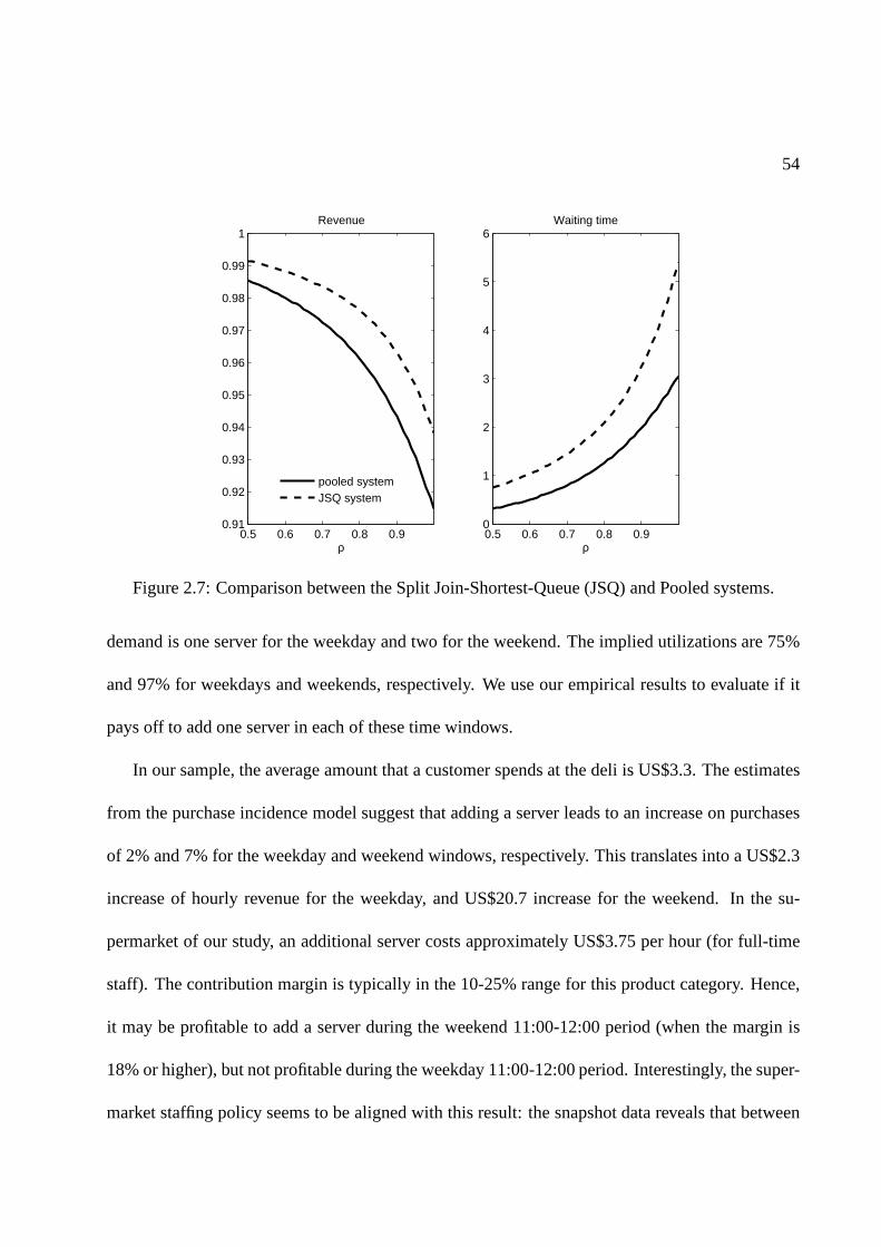
54

0.5 0.6 0.7 0.8 0.90.91

0.92

0.93

0.94

0.95

0.96

0.97

0.98

0.99

1

ρ

Revenue

pooled systemJSQ system

0.5 0.6 0.7 0.8 0.90

1

2

3

4

5

6Waiting time

ρ

Figure 2.7: Comparison between the Split Join-Shortest-Queue (JSQ) and Pooled systems.

demand is one server for the weekday and two for the weekend. The implied utilizations are 75%

and 97% for weekdays and weekends, respectively. We use our empirical results to evaluate if it

pays off to add one server in each of these time windows.

In our sample, the average amount that a customer spends at the deli is US$3.3. The estimates

from the purchase incidence model suggest that adding a server leads to an increase on purchases

of 2% and 7% for the weekday and weekend windows, respectively. This translates into a US$2.3

increase of hourly revenue for the weekday, and US$20.7 increase for the weekend. In the su-

permarket of our study, an additional server costs approximately US$3.75 per hour (for full-time

staff). The contribution margin is typically in the 10-25% range for this product category. Hence,

it may be profitable to add a server during the weekend 11:00-12:00 period (when the margin is

18% or higher), but not profitable during the weekday 11:00-12:00 period. Interestingly, the super-

market staffing policy seems to be aligned with this result: the snapshot data reveals that between

55

30-40% of the time the deli had a single server staffed duringthe weekday hour whereas for the

weekend more than 75% of the snapshots showed 3 or more servers.14

2.5.3 Implications for Category Pricing

The empirical results suggest that customers who are more sensitive to prices are less likely to

change their probability of purchasing fresh deli productswhen the length of the queue increases.

This can have important implications for the pricing of products under congestion effects, as we

show in the following illustrative example.

Consider two vertically differentiated products, H and L, of high and low quality respectively,

with respective pricespH > pL. Customers arrive according to a Poisson process to join an

M/M/1 queue to buy at most one of these two products. Following model (2.3.2), customer

preferences are described by a MNL model, where the utility for customeri if buying product

j ∈ L,H is given byUij = δj − βpi pj − βq

iQ + θi + ǫij . Customer may also choose not to join

the queue and get a utility equal toUi0 = ǫi0. In this RUM,δj denotes the quality of the product

andQ is a r.v. representing the queue length observed by the customer upon arrival. Customers

have heterogeneous price and waiting sensitivity characterized by the parametersβpi andβq

i . In

particular, heterogeneity is modeled through two discretesegments,s = 1, 2 with low and high

price sensitivity, respectively, and each segment accounts for 50% of the customer population

(later in this section we will also consider a continuous heterogeneity distribution based on our

empirical results). Letβp1 andβp

2 be the price coefficients for these segments, with0 < βp1 < βp

2 .

14The revenue increase was estimated using specification V from table 2.4. We repeated the analysis using a modelwhere customers also account for the number of employees staffed and the results are similar.

56

In addition, the waiting sensitivityβqi , is a random coefficient that can take two values:ωh with

probabilityrs andωl with probability1− rs, wheres denotes the customer segment andωl < ωh.

This characterization allows for price and waiting sensitivity to be correlated: ifr1 > r2, then a

customer with low price sensitivity is more likely to be morewaiting-sensitive; ifr1 = r2 then

there is no correlation.

Consider first a setting with no congestion so that Q is alwayszero (for example, if there is

ample service capacity). For illustration purposes, we fixed the parameters as follows:δH =

15, pH = 5, δL = 5, pL = 1.5, βp1 = 1, θ1 = 0, βp

2 = 10, θ2 = 12. In this example,

the difference in quality and prices between the two products is sufficiently large so that most of

the price sensitive customers (s = 2) buy the low quality productL. Moreover, define the cross

price elasticity of demandEHL as the percent increase in sales ofH product from increasing the

price ofL by 1%, and vice-versa forELH . In this numerical example, we allow for significant

heterogeneity with respect to price sensitivity such that,in the absence of congestion, the cross

elasticities between the two products are close to zero (to be exact,EHL = 0.002, ELH = 0.008).

Now consider the case where customers observe queues. This generates an externality: in-

creasing the demand of one product generates longer queues,which decreases the utility of some

customers who may in turn decide not to purchase. Hence, lowering the price of one product in-

creases congestion and thereby has an indirect effect on thedemand of the other product, which

we refer to as theindirect cross elasticity effect.

We now show how customer heterogeneity and negative correlation between price and waiting

sensitivity can increase the magnitude of the indirect cross elasticity between the two products.

We parametrized the waiting sensitivity of each segment asωl = 1.25 − 0.5∆ andωh = 1.25 +

57

0.5∆, where∆ is a measure of heterogeneity in waiting sensitivity. We also varied the conditional

probabilitiesr1 andr2 to vary the correlation between waiting and price sensitivity while keeping

the marginal distribution of waiting sensitivity constant(50% ωl and 50%ωh). Fixing all the

parameters of the model (including pricespH andpL), it is possible to calculate the stationary

probabilities of the queue lengthQ. Using the RUM together with this stationary distribution it is

then possible to calculate the share of each product (definedas the fraction of arriving customers

that buy each product). Applying finite differences with respect to prices, one can then calculate

cross elasticities that account for the indirect effect through congestion.

Based on this approach, we evaluated the cross elasticity ofthe demand for the H product

when changing the price of the L product (EHL) for different degrees of heterogeneity in customer

sensitivity to wait (∆) and several correlation patterns. The results of this numerical experiment

are presented in Table 2.6. Note that in the absence of heterogeneity– that is,∆ = 0 – the cross-

price elasticity is low: the two products H and L appeal to different customer segments and there

is little substitution between them. However, adding heterogeneity and correlation can lead to a

different effect. In the presence of heterogeneity, anegativecorrelation between price and waiting

sensitivity increasesEHL, showing that theindirect cross-elasticity increases when the waiting

sensitive customers are also the least sensitive to price. The changes in cross-elasticity due to

correlation can become quite large for higher degrees of customer heterogeneity. In the example,

when∆ = 2, the cross elasticity changes from 0.011 to 0.735 when moving from positive to

negative correlation patterns.

We now discuss the intuition behind the patterns observed inthe example of Table 2.6. When

there is heterogeneity in price sensitivity, lowering the price of the L product attracts customers

58

Correlation between price and waiting sensitivityHeterogeneity -0.9 -0.5 0 0.5 0.9

∆ = 0.0 - - 0.042 - -∆ = 1.0 0.342 0.228 0.120 0.047 0.010∆ = 2.0 0.735 0.447 0.209 0.070 0.011

Table 2.6: Cross-price elasticities describing changes inthe probability of purchase of the highprice product (H) from changes in the price of the low price product (L).

who were not purchasing before the price reduction (as opposed to cannibalizing the sales of the

H product). Due to this increase in traffic, congestion in thequeue increases, generating longer

waiting times for all customers. But when price and waiting sensitivity are negatively correlated,

the disutility generated by the congestion will be higher for the less price sensitive customers

and they will be more likely to walk away after the price reduction in L. Since a larger portion

of the demand for the H product comes from the less price sensitive buyers, the indirect cross-

price elasticity will increase as the correlation between price and waiting sensitivity becomes more

negative.

Although the above example uses discrete customer segments, similar effects occur when con-

sidering heterogeneity described through a continuous distribution, as in our empirical model.

Similar to the previous discrete case example, we assume theutility for customeri to purchasej is

given byUij = δj − βpi pj + f(βq

i , Q) + θi. But now the queue effect is specified by the quadratic

form with random coefficients for(βp, βq, θ) which are normally distributed with the same covari-

ance matrix as the one estimated in Table 2.5. PricespL andpH are picked to reflect the true price

of high end and low end products, andλ to reflect the empirical average arrival rate in the deli

session. In this case, our calculation shows a cross price elasticity equal toEHL = 0.81. In a

counter-factual that forces the waiting sensitivityβq to be independent of the other random coef-

59

ficients(βp, θ), the price elasticityEHL drops to 0.083, one order of magnitude smaller, showing

qualitatively similar results to those from the discrete heterogeneity example.

In summary, the relationship between price and waiting sensitivity is an important factor affect-

ing the prices in a product category when congestion effectsare present. Congestion can induce

price-demand interactions among products which in the absence of congestion would have a low

direct cross price-elasticity of demand. Our analysis illustrates how heterogeneity and negative cor-

relation between price and waiting sensitivity can exacerbate these interactions through stronger

indirect cross-elasticity effects. This can have important implications on how to set prices in the

presence of congestion.

2.6 Conclusions

In this study, we use a new data set that links the purchase history of customers in a supermarket

with objective service level measures to study how an important component of the service experi-

ence – waiting in queue – affects customer purchasing behavior.

An important contribution of this study is methodological.An existing barrier to study the

impact of service levels on customer buying behavior in retail environments comes from the lack

of objective data on waiting time and other customer servicemetrics. This work uses a novel data

collection technique to gather high frequency store operational metrics related to the actual level

of service delivered to customers. Due to the periodic nature of these data, an important challenge

arises in linking the store operational data with actual customer transactions. We develop a new

econometric approach that relies on queuing theory to inferthe level of service associated with each

60

customer transaction. In our view, this methodology could be extended to other contexts where

periodic service level metrics and customer transaction data are available. This methodology also

enables us to estimate a comprehensive descriptive model ofhow waiting in queue affects customer

purchase decisions. Based on this model we provide useful prescriptions for the management of

queues and other important aspects of service management inretail. In this regard, a contribution of

our work is to measure the overall impact of the state of the queue on customer purchase incidence,

thereby attaching an economic value to the level of service provided. This value of service together

with an estimate of the relevant operating costs can be used to determine an optimal target service

level, a useful input for capacity and staffing decisions.

Second, our approach empirically determines the most important factors in a queuing system

that influence customer behavior. The results suggest that customers seem to focus primarily on

the length of the line when deciding to join a queue, whereas the number of servers attending the

queue, which determines the speed at which the queue advances, has a much smaller impact on

customers’ decisions. This has implications for the designof a queuing system. For example,

although there are several benefits of pooling queues, the results in this study suggest that some

precautions should be taken. In moving towards a pooled system, it may be critical to provide

information about the expected waiting time so that customers are not drawn away by longer

queues. In addition, our empirical analysis provides strong evidence that the effect of waiting

on customer purchases is non-linear. Hence, measuring extremes in the waiting distribution – for

example, the fraction of the time that 10 or more customers are waiting in queue – may be more

appropriate than using average waiting time to evaluate thesystem’s performance.

Third, our econometric model can be used to segment customers based on their waiting and

61

price sensitivities. The results show that there is indeed asubstantial degree of heterogeneity in how

customers react to waiting and price, and moreover, the waiting and price sensitivity are negatively

correlated. This has important implications for the pricing of a product category where congestion

effects are present. Lowering prices for one product increases demand for that alternative, but

also raises congestion generating a negative externality for the demand of other products from

that category. Heterogeneity and negative correlation in price and waiting sensitivity exacerbates

this externality, and therefore should be accounted for in category pricing decisions. We hope

that this empirical finding fosters future analytical work to study further implications of customer

heterogeneity on pricing decisions under congestion.

Finally, our study has some limitations that could be explored in future research. For example,

our analysis focuses on studying the short term implications of queues by looking at how customer

purchases are affected during a store visit. There could be long-term effects whereby a negative

service experience also influences future customer purchases, for example, the frequency of visits

and retention. Another possible extension would be to measure how observable customer charac-

teristics – such as demographics – are related to their sensitivity to wait. This would be useful, for

example, to prescribe target service levels for a new store based on the demographics of the mar-

ket. Competition could also be an important aspect to consider; this would probably require data

from multiple markets to study how market structure mediates the effect of queues on customer

purchases.

On a final note, this study highlights the importance of integrating advanced methodologies

from the fields of operations management and marketing. We hope that this work stimulates further

research on the interface between these two academic disciplines.

62

Chapter 3

Prioritizing Burn-Injured Patients During a

Disaster

3.1 Introduction

Following the terrorist attacks on September 11, 2001, the US government initiated the develop-

ment of disaster plans for resource allocation in a bioterrorism or other mass casualty event (AHRQ

Brief 2006). There are many important operational issues tobe considered in catastrophic events.

Supply chain management as well as facility location and staffing are important factors when de-

termining how to dispense antibiotics and other counter measures (Bravata et al. 2006, Lee et al.

2009). In the event of a nuclear attack, guidance is needed onwhether people should evacuate or

take shelter-in-place (Wein et al. 2010). For large events,a critical consideration is how to deter-

mine who gets priority for limited resources (Argon et al. 2008). In this work, we focus on disaster

planning for burn victims.

63

Patients with severe burns require specialized care due to their susceptibility to infection and

potential complications due to inhalation injury and/or shock. Specialized treatments, including

skin grafting surgeries and highly specialized wound care,are best delivered in burn centers and

are important in increasing the likelihood of survival and reducing complications and adverse out-

comes (Committee on Trauma 1999).

There have been a number of events in recent years which wouldqualify as ‘burn disasters’.

For instance, in 2003, 493 people were caught in a fire at a Rhode Island night club and 215 of

them required treatment at a hospital (Mahoney et al. 2005).During this event, the trauma floor

of the Rhode Island Hospital was converted to a burn center inorder to provide the necessary

resources to care for the victims. Other burn disasters weredue to terrorist attacks such as those in

Bali in 2002 and 2005 and the Jakarta Marriott Hotel bombing in 2003 (Chim et al. 2007). In these

events, some patients were transported to Australia and Singapore for treatment. In all of these

burn disaster events, there were more burn victims than could be adequately treated by existing

burn centers and other measures were required to provide care for all the patients.

To prepare for the possibility of a burn disaster occurring in American cities, the Federal Health

Resources and Services Administration (HRSA) has developed standards for metropolitan areas.

These include a mandate to develop a plan to care for 50 burn-injured patients per million people,

beyond which a national plan would be activated to transportpatients to other locations. For most

metropolitan areas, such as New York City (NYC), this mandate exceeds the current burn center

capacity. Hence, there is a need to develop a burn disaster plan for the triage, transportation,

and other related issues involved in managing an overloadedsituation. The plan must include

“guidelines and other materials for the management and treatment of selected burn-injured patients

64

for the first three to five days in non-burn centers in the eventof a large chemical or explosive event”

(Fund for Public Health in New York, Inc. 2005). The three to five day horizon is consistent with

clinical guidelines for the surgical treatment of burn victims.

There are currently 71 burn beds in NYC, which is typically a sufficient number to care for the

normal demands of burn-injured patients. During periods ofvery high demand, burn centers can

provide ‘surge’ capacity of about 50% over their normal capacity by treating patients in other units

of the hospital using burn service personnel. There are an additional 69 burn center beds in the

60 mile radius surrounding NYC (including New Jersey and Connecticut), bringing the total surge

bed capacity in the greater metropolitan area to 210. Based on 2000 US census data, the federal

mandate of 50 patients per million people corresponds to being able to care for 400 NYC patients

(Yurt et al. 2008), which far exceeds the surge capacity of 210 beds.

Consequently, a task force of burn specialists, emergency medicine physicians, hospital admin-

istrators and NYC officials was created to develop a burn disaster response plan (Yurt et al. 2008).

To do this, they identified hospitals which do not have burn centers, but have agreed to assist in

stabilizing burn-injured patients until they can be transferred to a burn center.

The main focus of the work presented in this study was to develop a detailed triage plan for

prioritizing burn-injured patients for transfer to burn beds in order to maximize the benefit gained

across all patients from receiving specialized burn care. More specifically, the NYC Task Force

asked us to identify methods for refining and improving the initial triage system presented in Yurt

et al. (2008) which uses broad categories based on age and burn severity to classify patients. We

propose a new triage algorithm which includes individual survivability estimates and incorporates

patient length-of-stay as well as specific comorbidities which have significant impact on the triage

65

performance. Based on data from previous burn catastrophes, we demonstrate that this new al-

gorithm results in significantly better performance than other candidate triage methodologies. We

also consider the feasibility of the proposed disaster planto provide care in burn units for the vast

majority of the 400 burn victims mandated by the federal guidelines for NYC. Our analyses sug-

gest that it is highly improbable that most burn-injured patients will be able to be transferred to

burn beds within the prescribed 3 to 5 day stabilization period. This suggests that federal assistance

may be necessary even when the total number of burn-injured patients is much smaller than the 50

per million population guideline. Though this work focuseson improving the initial plan for NYC

as outlined in Yurt et al. (2008), it provides useful insights for the development of burn disaster

plans in other cities.

The rest of the chapter is organized as follows. Section 3.2 provides background on burn

care and the initial disaster plan established in 2008 (Yurtet al. 2008). Section 3.3 presents our

stochastic model and optimization framework. Due to the complexity of the problem, we develop

a heuristic prioritization algorithm. In Section 3.4, we discuss how to translate our model into

practice and how to include two additional key factors: length-of-stay (LOS) and comorbidities.

In Section 3.5, we show that including these factors can improve triage performance, measured

in expected number of additional survivors, by up to 15%. Section 3.6 considers the feasibility

of caring for all 400 patients in Tier 1 burn beds. We find that the ability to treat all burn-injured

patients within the first 3 to 5 days is highly dependent on thetype of event and the severity of the

patients. Finally, we provide some concluding remarks in Section 3.7.

66

3.2 Background

Careful triage of patients in any disaster scenario is critical in effectively utilizing limited health-

care resources. It is particularly vital in a burn disaster due to the specific and nuanced care required

by burn-injured patients.

3.2.1 Burn Care

Figure 3.1 summarizes the typical treatment timeline for a burn-injured patient. During the first

hours after injury, care for seriously injured burn patients focuses upon stabilization, resuscitation,

and wound assessment. In the ensuing days, supportive care is continued, and, if possible, the

patient is taken to the operating room for wound debridementand grafting as tolerated. It is rec-

ommended that such surgeries are performed by burn specialists. While there is limited literature

on the impact of delayed transfer to burn centers, it is widely accepted that it is not likely that there

will be worse outcomes as long as patients are cared for by burn specialists within the first 3 to 5

days. Delayed treatment from burn specialists much longer than 5 days may result in worse out-

comes if wounds are not properly cared for and begin to exhibit symptoms of infection and other

clinical complications (Sheridan et al. 1999). Note that patients who suffer from extensive burn

wounds may require multiple surgeries with recovery times between them because each skin graft

covers a limited area.

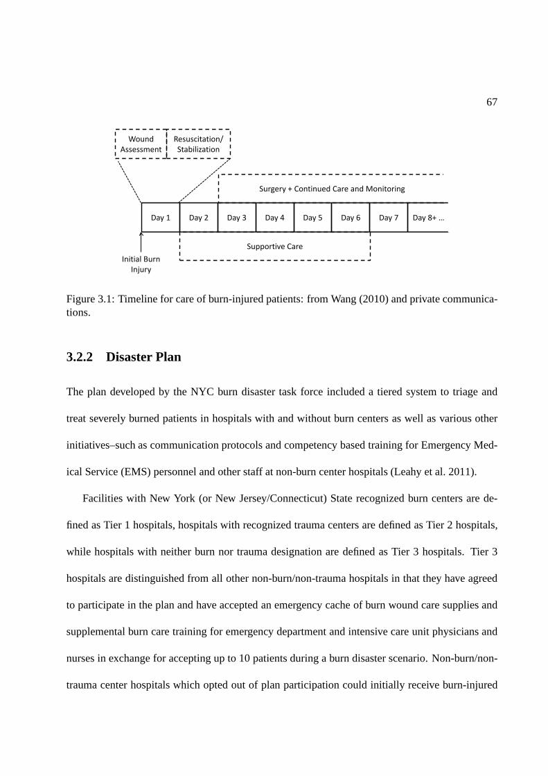
67

Wound

Assessment

Resuscitation/

Stabilization

Supportive Care

Surgery + Continued Care and Monitoring

Day 1 Day 2 Day 3 Day 4 Day 5 Day 6 Day 7 Day 8+ …

Initial Burn

Injury

Figure 3.1: Timeline for care of burn-injured patients: from Wang (2010) and private communica-tions.

3.2.2 Disaster Plan

The plan developed by the NYC burn disaster task force included a tiered system to triage and

treat severely burned patients in hospitals with and without burn centers as well as various other

initiatives–such as communication protocols and competency based training for Emergency Med-

ical Service (EMS) personnel and other staff at non-burn center hospitals (Leahy et al. 2011).

Facilities with New York (or New Jersey/Connecticut) Staterecognized burn centers are de-

fined as Tier 1 hospitals, hospitals with recognized trauma centers are defined as Tier 2 hospitals,

while hospitals with neither burn nor trauma designation are defined as Tier 3 hospitals. Tier 3

hospitals are distinguished from all other non-burn/non-trauma hospitals in that they have agreed

to participate in the plan and have accepted an emergency cache of burn wound care supplies and

supplemental burn care training for emergency department and intensive care unit physicians and

nurses in exchange for accepting up to 10 patients during a burn disaster scenario. Non-burn/non-

trauma center hospitals which opted out of plan participation could initially receive burn-injured

68

patients who self-refer or are transported to these hospitals because of the availability of resources

and/or proximity to the scene, but would then be transferredto participating hospitals.

While some catastrophes may develop over the course of a few days, the Task Force was

primarily concerned with disasters which create a sudden large surge in patient arrivals such as

those caused by a bombing or large fire. In such events, patients arrive to hospitals within a few

hours and certainly by the end of the first day. The timescale of patient arrivals is extremely short

in relation to the average length-of-stay of burn-injured patients, which is 13 days; hence, the Task

Force focused on a reasonable worse-case scenario where allpatients arrive at the beginning of the

horizon.

As patients arrive to hospital emergency departments, theywill be classified and given a triage

score after examination. Based on these assessments, some patients will be transferredinto Tier

1 hospitals while others may be transferredout so as to reflect the prioritization scheme of the

burn disaster plan. The Virtual Burn Consultation Center (VBCC) is a centralized tracking system

which will be used to coordinate such interfacility transportation (Leahy et al. 2011).

Though the initial transportation and transfer logistics are part of the overall burn disaster plan

developed by the Task Force, the major focus of the work described here was the development

of a triage algorithm to determine the prioritization of patients during the initial assessment and

reassignment period as well as for the transfer of patients who are provided their initial care in Tier

2 and 3 hospitals, but who will be transferred to Tier 1 hospitals as those beds become available. It

is important to note that any triage algorithm is a decision aid which is meant to provide guidance

to clinicians who ultimately make the actual determinationof patient priorities. However, given the

69

number of relevant factors, an algorithm is necessary to deal with the complexity and it is assumed

that it will be followed in most cases.

The total surge capacity of Tier 1 hospitals’ burn beds in thegreater metropolitan area is 210.

If there are more than 210 burn-injured patients, Tier 2 and 3hospitals will be used to stabilize

patients until they can be transferred into a Tier 1 hospital, with preference given to Tier 2 hospi-

tals. Because burn-injured patients may require resuscitation, cardiopulmonary stabilization, and

emergency care procedures prior to skin grafting surgeries, the Tier 2 and 3 hospitals were selected

based on their ability to stabilize and provide the basic wound care required within the first few

days. By day 3, most burn-injured patients should receive specialized burn care in a Tier 1 hospi-

tal. Some patients are less delay sensitive and can wait up to5 days to receive Tier 1 care without

incurring harm. If the total number of burn-injured patients is estimated to be beyond the number

that can be admitted to treatment in a specialized burn bed byday5, a national plan which would

involve air transport to other metropolitan areas would go into effect. Since such a national plan

would be very costly, complex, and potentially dangerous for many burn victims, the objective of

the Task Force was to devise a plan that could provide for the treatment of up to 400 burn-injured

patients in Tier 1 facilities within 3 to 5 days.

There are three main factors which affect patient survivability and length-of-stay: Burn size (as

measured by Total Body Surface Area (TBSA)), age and inhalation injury (IHI). The triage deci-

sion matrix from Saffle et al. (2005) classifies patients based on likelihood of survival. Patients who

are expected to survive and have good outcomes without requiring burn center admission are cate-

gorized as Outpatients; Very High patients who are treated in a burn center have survival likelihood

≥ 90% and require a length-of-stay (LOS) between 14-21 days and 1-2 surgical procedures; High

70

patients also have high survival likelihood≥ 90% but require more aggressive care with multiple

surgeries and LOS greater than 21 days; Medium patients havesurvival likelihood50 − 90% and

require multiple surgeries and LOS of greater than 21 days; Low patients have survival likelihood

less than50% even with aggressive treatment; Expectant patients have survival likelihood less than

10%. LOS is defined as the duration of time in the burn unit until discharge.

This initial matrix was modified to include the presence of inhalation injury (Yurt et al. 2008).

If the goal were simply to maximize the expected number of survivors, patients with the highest

probability of survival would be favored for access to Tier 1burn beds. However, priority for

Tier 1 beds was determined under the premise that burn beds should first be given to patients

who are severe enough that they will benefit significantly from specialized burn care, but not so

severe that they are unlikely to survive even if provided with the prescribed treatment. Hence,

the Burn Disaster Triage matrix was based on the clinical judgment of burn treatment experts

as to which patients wouldbenefit mostfrom specialized burn care. In this determination, the

least injured patients were deemed to have a very high likelihood of survival, even if they are not

admitted to a burn unit within the 5 day horizon mentioned above and so they were not included

in the highest priority group. The modified decision matrix,shown in Figure 3.2, creates a block

priority structure that was the starting point for the work described in this study. A patient’stype

determines his priority for Tier 1 beds. All patients categorized as Outpatient are not considered

in the burn disaster infrastructure.Type 1patients (in gray) are given first priority for Tier 1 beds.

These patients consist of Very High, High and Medium patients from Saffle et al. (2005) and were

identified as the types of patients who are most likely to benefit from being treated in a burn center.

All other patients (labeled with Tier 2/3 in the matrix) havelower priority for transfer into Tier 1

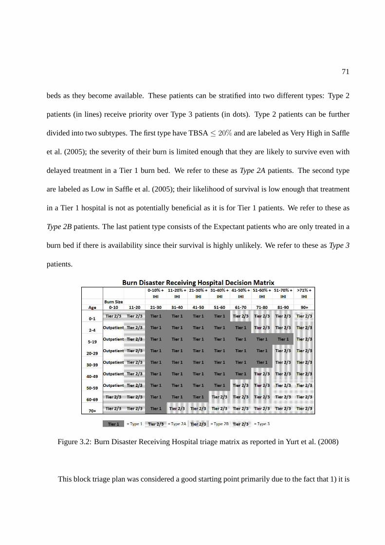
71

beds as they become available. These patients can be stratified into two different types: Type 2

patients (in lines) receive priority over Type 3 patients (in dots). Type 2 patients can be further

divided into two subtypes. The first type have TBSA≤ 20% and are labeled as Very High in Saffle

et al. (2005); the severity of their burn is limited enough that they are likely to survive even with

delayed treatment in a Tier 1 burn bed. We refer to these asType 2Apatients. The second type

are labeled as Low in Saffle et al. (2005); their likelihood ofsurvival is low enough that treatment

in a Tier 1 hospital is not as potentially beneficial as it is for Tier 1 patients. We refer to these as

Type 2Bpatients. The last patient type consists of the Expectant patients who are only treated in a

burn bed if there is availability since their survival is highly unlikely. We refer to these asType 3

patients.

Figure 3.2: Burn Disaster Receiving Hospital triage matrixas reported in Yurt et al. (2008)

This block triage plan was considered a good starting point primarily due to the fact that 1) it is

72

based on data from the National Burn Repository as well as theclinical judgment of experienced

burn clinicians and 2) it is simple and easy to implement. However, a major shortcoming of this

triage system is that it is a gross categorization scheme with three priority types: Type 1, 2, and 3.

If there are more Type 1 patients than there are Tier 1 beds, there are no guidelines to determine

which patients get priority. Similarly, as Tier 1 beds become available, there are no guidelines

to differentiate among the Type 2 and Type 3 patients. Finally, while this block plan is based on

expert opinion on patients’ expected increase in likelihood of survival due to treatment in a burn

unit, it does not incorporate any individual estimates of survival either with or without specialized

burn care. We discuss this issue in more detail later.

The goal of the work we were asked to perform by the NYC task force was to prioritize pa-

tients within these gross categories. In doing so, we decided to consider if and how to incorporate

comorbidities in the triage plan noting that comorbiditiescan significantly impact patient surviv-

ability and length-of-stay. As we discuss in subsequent sections, we also examined the implicit

assumptions of the original block matrix plan, and the feasibility of providing burn unit treatment

for all 400 burn victims within the designated time horizon.

3.2.3 Operations Literature

Patient triage, which is essentially a prioritization scheme, has generated substantial attention from

the operations research community. Classical index rule results from the scheduling literature (see

Pinedo (2008)) can often provide insight into how to manage patient triage. The well-known c-µ

rule minimizes holding costs in a variety of settings (Buyukkoc et al. 1985, van Mieghem 1995).

73

Saghafian et al. (2011) modifies this priority rule to incorporate a complexity measure for patient

triage in the Emergency Department.

Patient triage in disaster scenarios has the additional complication that, because the number of

patients exceeds the number of health resources (beds, nurses, physicians, etc.), some, or even

many, patients may not be able to receive treatment before they die, corresponding to patient

abandonment. Glazebrook et al. (2004) proposes a c-µ-like priority rule which maximizes reward

as the exponential abandonment rates go to zero. A similar priority rule is proposed in Argon et al.

(2008) for general service times and abandonment rates. What separates our work from these is

that we consider how to leverage the structure and timeline of the treatment of burn-injured patients

in designing a triage system. In doing so, we emphasize the need to combine mathematical rigor

with clinical relevance and judgment to encourage physician adoption.

One issue of great concern to the physicians is how to triage patients when their medical history

is unknown. In a classification scheme based on patient severity, the presence or lack of comorbidi-

ties can have substantial impact on a patient’s priority. Argon and Ziya (2009) proposes a triage

scheme to minimize long-run average waiting costs under imperfect customer classification. Each

patient is associated with a probability of being of higher priority and triage is done in decreasing

order of this probability. Our work also considers uncertainty in patient classification; however, it

may be possible to expend some effort, via tests or speaking to the patient, to extract information

about the presence of a particular comorbidity. Certainly,it is time consuming and costly to ex-

tract information onall possible comorbidities. Hence, we determine which, if any,comorbidities

are most important in assessing survival probabilities and/or length of stay. Finally, the objective

74

of our triage system is quite different as our time horizon isfinite given the criticality of treating

burn-injured patients within the first 3-5 days following injury.

Our goal in this work is to bring a systematic framework to a current, important and real world

problem. Triage plans, especially in disaster scenarios, are inherentlyqualitativeas decisions have

to be made quickly with limited data. The challenge is to bring mathematical rigor based on

incomplete data to an inherently clinical and subjective decision process.

3.3 Model and a Heuristic

The goal of a disaster triage plan is to use the limited resources available so as to maximize the

overall benefit to the affected population. Though in the case of burn patients, benefit can include

improvements with respect to scarring and disability, the most important performance metric is

clearly the increase in the likelihood of survival. Therefore, the ideal model for prioritizing patients

to burn beds would be one that maximizes the overall increasein the expected number of survivors

due to use of these beds. We describe such a model for the NYC burn disaster situation in this

section. As we explain in more detail in a subsequent section, we must infer these benefits due to

limitations in available data.

There areN patients who are eligible for treatment in one of theB Tier 1 burn beds at the

beginning of the horizon, whereB < N . We assume that there is sufficient capacity in the Tier

2/3 beds to accommodate all burn-injured patients not initially placed into a Tier 1 bed while they

wait to be transferred into a Tier 1 burn bed.

We assume that we know all patients’ probability of survivalif they do not receive timely care

75

in a Tier 1 bed as well as the increase in this probability if they do. We further assume that patients

fall into one of two classes which defines their delay tolerance for burn unit care. Specifically, a

Class 1 patient must be transferred to a Tier 1 bed within3 days in order to realize the associated

improvement in survivability while a Class 2 patient can remain in a Tier 2/3 bed for up to5 days

before being transferred to a Tier 1 bed without jeopardizing his probability of survival.

Each patienti ∈ 1, 2, . . . , N is defined by his class,Ci ∈ 1, 2, his increase in probability

of survival due to timely Tier 1 burn care,∆Pi, and his expected length-of-stay (LOS),Li. Though

we initially assume that patienti’s LOS is exponentially distributed with meanLi, we relax this

assumption later.

Let ti be the time at which patienti is transferred into one of theB beds at which time he

generates reward

∆Pi[1ti≤3,Ci=1 + 1ti≤5,Ci=2]

That is, a class1 patient who is transferred within his3 day delay tolerance will benefit∆Pi from

Tier 1 burn care. Note that not all class1 patients are necessarily Type1 patients. Likewise, a

class2 patient must be transferred within his5 day delay tolerance. Letti(π) be the (random) time

patienti is transferred into a Tier 1 burn bed under triage policyπ. Our objective is to select the

triage algorithm,π, which maximizes the total expected increase in the number of survivors due to

timely burn unit treatment.

maxπ

E

[

N∑

i=1

∆Pi[1ti(π)≤3,Ci=1 + 1ti(π)≤5,Ci=2]

]

(3.3.1)

76

3.3.1 Potential Triage Policies

If all patients had tocomplete, rather thanstart, treatment within the first 5 days, then a simple

index rule which prioritizes patients in decreasing order of the ratio between patient benefit, i.e.

increase in survivability, and expected LOS (∆Pi/Li), i.e. the incremental reward per day in the

burn center, would be optimal. This can be shown via a simple interchange argument. Such an

index rule leverages known results from the classical scheduling literature whereWeighted Shortest

Processing Time (WSPT) firstis optimal for a number of parallel processing scheduling problems

(see Pinedo (2008)).

Our problem has a modified constraint which requires class1 and2 patients tobegintreatment

within the first3 and5 days, respectively, in order to generate any reward. This makes our schedul-

ing problem substantially more difficult. In particular, one can map our scheduling problem with

objective (3.3.1) to a stochastic scheduling problem with an objective of minimizing the weighted

number of tardy jobs, where the weight for jobi is∆Pi and the due date is31Ci=1+51Ci=2+Si,

whereSi is the processing time for jobi. Hence, the job must start processing by timeT = 3 (or

5) days if he is class1 (or 2). If patient LOS were deterministic, i.e. ifSi = Li with probability1,

this problem would be NP-hard (Pinedo 2008). The most commonly used heuristic for the deter-

ministic problem is the WSPT index rule:∆Pi/Li. However, in the worst case, the performance

of this heuristic can be arbitrarily bad. In our stochastic model, the service times are independent

exponential random variables so the due dates are now randomand correlated with the service

times, adding additional complexity.

There are various results in the literature on minimizing expected weighted tardy jobs. More

77

general models, for instance with arbitrary deadlines or service times distribution, can be shown to

be NP-hard. In special cases, optimal policies are known. For instance, with i.i.d. due dates and

processing times, it is optimal to sequence jobs in order of weights (Boxma and Forst 1986). Forst

(2010) identifies conditions for optimality, which in our case would correspond to the optimality

of WPST if∆Pi ≥ ∆Pj if and only ifLi ≤ Lj . Unfortunately, this condition is too restrictive for

the burn triage problem and so WSPT is not necessarily optimal. In other cases, such as Jang and

Klein (2002), which examines a single machine with a common deterministic due date, heuristic

algorithms must be considered.

3.3.2 Proposed Heuristic

Given the inherent difficulty of solving for the optimal triage algorithm, we focus on a modified

version of the most commonly used heuristic which is to prioritize patients in decreasing order

of ∆Pi/Li. The average LOS of burn-injured patients is quite large (much more than 5 days),

as seen in Table 3.4. Consequently, the distinction betweenstartingversuscompletingtreatment

within the first 3 or 5 days is significant. Consider a simple example with two class2 patients and

one bed. Patient A has benefit potential 0.10 and expected LOSof 30 days. Patient B has benefit

potential 0.05 and expected LOS of 10 days. Using the WSPT heuristic, patient B gets priority

since0.05/10 > 0.10/30. With probability 0.3935, patient B completes before 5 days, and patient

A can also start treatment within the first 5 days. Hence, the expected benefit, i.e. number of

additional patients lives saved, by scheduling patient B first is0.0893 = 0.05 + 0.3935 ∗ 0.10. On

the other hand, the expected benefit by scheduling patient A first is0.1077 = 0.10+0.1535 ∗ 0.05.

Because these patients both have very long LOS, the likelihood of being able to start treatment for

78

the second patient is very low. Hence, it is better to start with the patient with the highest benefit

potential (patient A).

Consider a more general example with two patients and one bed. PatientA andB have benefit

potential∆PA and∆PB, respectively; they are both class1; their LOS,SA andSB, are exponen-

tially distributed with meanLA andLB. We consider the criteria such that patient A should be

given priority, i.e. under what conditions is the expected benefit larger when patient A is given

priority versus when patient B is given priority? This occurs when:

∆PA +∆PBFA(3) ≥ ∆PB +∆PAFB(3)

∆PA

1− FA(3)≥ ∆PB

1− FB(3)(3.3.2)

whereFi(x) = P (Si < x) is the cdf of an exponential random variable with meanLi. Hence,

patientA should be given priority if his index, ∆PA

P (SA≥3), is larger than patientB’s index, ∆PB

P (SB≥3).

Based on this analysis, our proposed heuristic algorithm isto prioritize patients in decreasing order

of the following triage index:

∆Pi

P (Si ≥ 3)= ∆Pie

3/Li (3.3.3)

This new triage index would give priority to patient A in the example given above where WSPT

gives priority to patient B. Hence, it has a higher expected benefit than WSPT. In general, the

proposed algorithm is not optimal. Consider the following example with three patients and one

bed. The patient parameters are summarized in Table 3.1. Patient A has the shortest expected

LOS, but also the lowest benefit potential. However, given the short horizon of 3 days, patientA

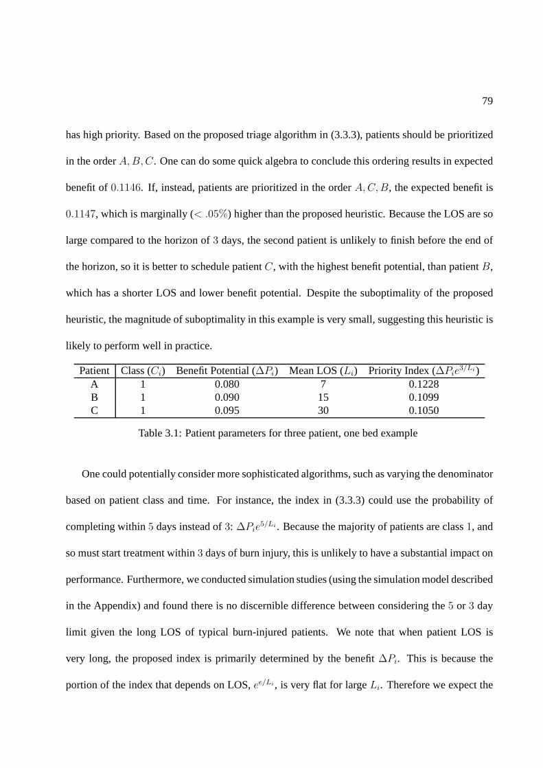
79

has high priority. Based on the proposed triage algorithm in(3.3.3), patients should be prioritized

in the orderA,B,C. One can do some quick algebra to conclude this ordering results in expected

benefit of0.1146. If, instead, patients are prioritized in the orderA,C,B, the expected benefit is

0.1147, which is marginally (< .05%) higher than the proposed heuristic. Because the LOS are so

large compared to the horizon of3 days, the second patient is unlikely to finish before the end of

the horizon, so it is better to schedule patientC, with the highest benefit potential, than patientB,

which has a shorter LOS and lower benefit potential. Despite the suboptimality of the proposed

heuristic, the magnitude of suboptimality in this example is very small, suggesting this heuristic is

likely to perform well in practice.

Patient Class (Ci) Benefit Potential (∆Pi) Mean LOS (Li) Priority Index (∆Pie3/Li)

A 1 0.080 7 0.1228B 1 0.090 15 0.1099C 1 0.095 30 0.1050

Table 3.1: Patient parameters for three patient, one bed example

One could potentially consider more sophisticated algorithms, such as varying the denominator

based on patient class and time. For instance, the index in (3.3.3) could use the probability of

completing within5 days instead of3: ∆Pie5/Li . Because the majority of patients are class1, and

so must start treatment within3 days of burn injury, this is unlikely to have a substantial impact on

performance. Furthermore, we conducted simulation studies (using the simulation model described

in the Appendix) and found there is no discernible difference between considering the5 or 3 day

limit given the long LOS of typical burn-injured patients. We note that when patient LOS is

very long, the proposed index is primarily determined by thebenefit∆Pi. This is because the

portion of the index that depends on LOS,ee/Li, is very flat for largeLi. Therefore we expect the

80

suboptimality to be small in such cases. Finally, our proposed triage index in (3.3.3) is relatively

simple which makes it ideal for real world implementation.

A major challenge in actually using the proposed model and heuristic is the lack of appropriate

data. Quantifying the benefit,∆Pi, for each patient is not possible as there is no source of dataon

the likelihood of survival for burn patients not treated in aburn unit since almost all burn patients

are transferred to burn units for care. The National Burn Repository only maintains outcome data

for burn-injured patients who are treated in burn units. In the next section, we describe several

approaches for dealing with this data limitation.

3.4 Parameter Estimation and Model Refinement

3.4.1 Parameter Estimation

We now consider how to estimate the parameters for our proposed algorithm for use in the burn

disaster plan. In particular, we need to determine the benefit, expected LOS, and class, (∆Pi, Li,

andCi) for each patienti.

Survival Probability: We begin with the likelihood of survival from which we infer the benefit

of Tier 1 care. The nominal survival probability can be estimated using the TIMM model in Osler

et al. (2010), which is based on a non-linear function of patient’s age, burn size, and presence of

inhalation injury. This provides a continuous measure for mortality rate rather than the previously

used coarse matrix blocks based on age and severity of burn asin Saffle et al. (2005). More specif-

ically, TIMM uses the following logistic regression model to predict the thermal injury probability

81

of survival:

Pi =1

1 + eβ0+β1TBSA+β2Age+β3IHI+β4

√TBSA+β5

√Age+β6TBSA×IHI+β7Age×IHI+β8TBSA×Age/100

(3.4.1)

where TBSA is Total Burn Surface Area and is measured in percentage; Age is measured in years;

and inhalation injury (IHI) is a binary variable. The coefficients of the function are estimated from

the National Burn Repository Data Set (39,888 Patients), and are listed in Table 3.2. We assume

this survival probability decreases for patients who are admitted to a burn center after the initial 3

or 5 day window. This decrease captures thebenefitof Tier 1 burn care.

k Variable βk0 Constant -7.63881 TBSA 0.03682 Age 0.13603 IHI 3.33294

√TBSA 0.4839

5√Age -0.8158

6 TBSA× IHI -0.02627 Age× IHI -0.02228 TBSA×Age/100 0.0236

Table 3.2: TIMM coefficients as reported in Osler et al. (2010)

Benefit: There is no generally accepted model for how patients’ conditions evolve over time

depending on the type of treatment given. This is primarily because of the limited quantitative data

on the reduction in mortality when transferred into a burn center. Sheridan et al. (1999) is one of

the few works which look at the impact of delayed transfers; however, the study only includes a

total of 16 pediatric patients with delayed treatment of up to 44 days. The small sample size, the

specialized population and the often long delays involved make it impossible to use their results in

82

our model. As such, we infer the benefit of burn center care based on the New York City plan and

the judgment of the clinicians on the Task Force.

In order to translate our objective into the increase in number of survivors, we introduce the

following construct: Each patient has a deterioration factorw ∈ [0, 1], which represents therelative

benefit of Tier 1 burn care, i.e. the patient’s survivabilitywill decrease byw if he is not transferred

to a burn bed before his delay tolerance expires. A patient’sabsolutebenefit is then:

∆Pi = wiPi

The deterioration factors are chosen so that, in general, priority is given to Type 1 patients, followed

by Type 2 patients, and finally Type 3 patients. This is to be consistent with the clinical judgment

used to establish the initial triage matrix. In that spirit we assume that, within each patient type,

the relative benefit of Tier 1 treatment is identical. As such, we must derive 4 deterioration factors:

w1, w2A, w2B andw3. Because the survivability of patients within each type canvary quite a bit,

the absolute benefit,∆Pi, will differ across patients of the same type.

We start with an estimate of the range ofw2A and derive ranges for the remaining patient

types. The survivability for Type 2A patients is very high; hence, even a small deterioration factor

translates into a large benefit. As such, and supported by clinical judgment, we assume this factor

is between 5-15%. Because the absolute benefit for Type 1 patients is assumed to be the largest

(resulting in their initial priority for Tier 1 treatment),we require thatw1 > w2A. More generally,

givenw2A, the ranges of deterioration factors for the other patient types are estimated as to be

consistent with the priorities given by the Triage Matrix inFigure 3.2. These deterioration factors

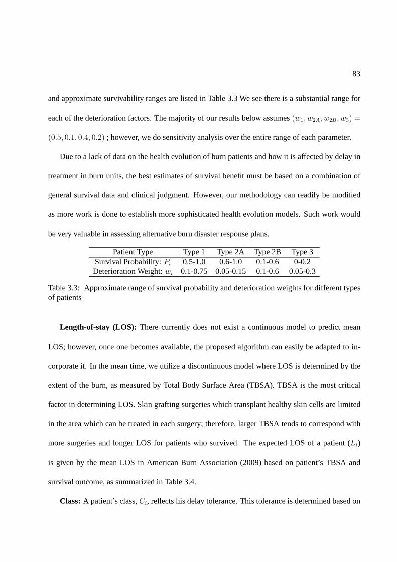
83

and approximate survivability ranges are listed in Table 3.3 We see there is a substantial range for

each of the deterioration factors. The majority of our results below assumes(w1, w2A, w2B, w3) =

(0.5, 0.1, 0.4, 0.2) ; however, we do sensitivity analysis over the entire range of each parameter.

Due to a lack of data on the health evolution of burn patients and how it is affected by delay in

treatment in burn units, the best estimates of survival benefit must be based on a combination of

general survival data and clinical judgment. However, our methodology can readily be modified

as more work is done to establish more sophisticated health evolution models. Such work would

be very valuable in assessing alternative burn disaster response plans.

Patient Type Type 1 Type 2A Type 2B Type 3Survival Probability:Pi 0.5-1.0 0.6-1.0 0.1-0.6 0-0.2Deterioration Weight:wi 0.1-0.75 0.05-0.15 0.1-0.6 0.05-0.3

Table 3.3: Approximate range of survival probability and deterioration weights for different typesof patients

Length-of-stay (LOS): There currently does not exist a continuous model to predictmean

LOS; however, once one becomes available, the proposed algorithm can easily be adapted to in-

corporate it. In the mean time, we utilize a discontinuous model where LOS is determined by the

extent of the burn, as measured by Total Body Surface Area (TBSA). TBSA is the most critical

factor in determining LOS. Skin grafting surgeries which transplant healthy skin cells are limited

in the area which can be treated in each surgery; therefore, larger TBSA tends to correspond with

more surgeries and longer LOS for patients who survived. Theexpected LOS of a patient (Li)

is given by the mean LOS in American Burn Association (2009) based on patient’s TBSA and

survival outcome, as summarized in Table 3.4.

Class:A patient’s class,Ci, reflects his delay tolerance. This tolerance is determinedbased on

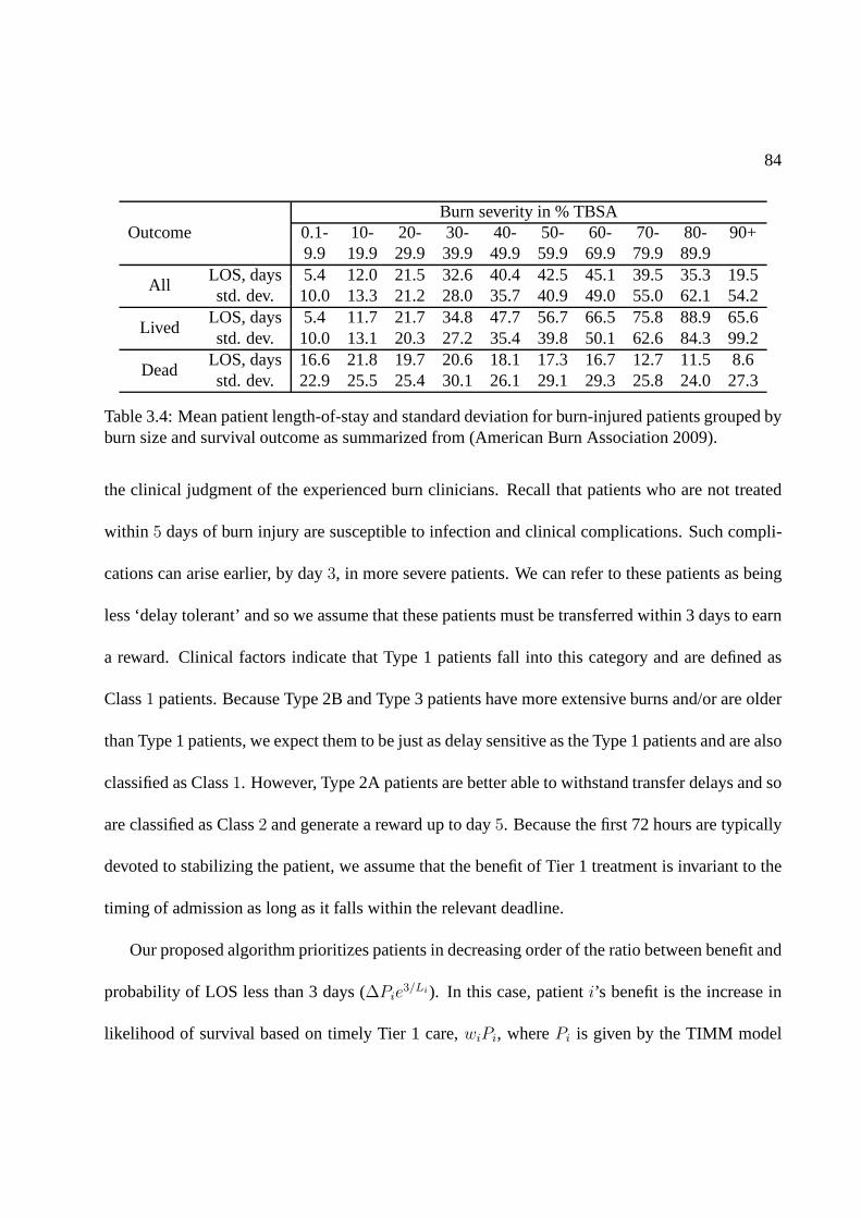
84

Burn severity in % TBSAOutcome 0.1- 10- 20- 30- 40- 50- 60- 70- 80- 90+

9.9 19.9 29.9 39.9 49.9 59.9 69.9 79.9 89.9

AllLOS, days 5.4 12.0 21.5 32.6 40.4 42.5 45.1 39.5 35.3 19.5std. dev. 10.0 13.3 21.2 28.0 35.7 40.9 49.0 55.0 62.1 54.2

LivedLOS, days 5.4 11.7 21.7 34.8 47.7 56.7 66.5 75.8 88.9 65.6std. dev. 10.0 13.1 20.3 27.2 35.4 39.8 50.1 62.6 84.3 99.2

DeadLOS, days 16.6 21.8 19.7 20.6 18.1 17.3 16.7 12.7 11.5 8.6std. dev. 22.9 25.5 25.4 30.1 26.1 29.1 29.3 25.8 24.0 27.3

Table 3.4: Mean patient length-of-stay and standard deviation for burn-injured patients grouped byburn size and survival outcome as summarized from (AmericanBurn Association 2009).

the clinical judgment of the experienced burn clinicians. Recall that patients who are not treated

within 5 days of burn injury are susceptible to infection and clinical complications. Such compli-

cations can arise earlier, by day3, in more severe patients. We can refer to these patients as being

less ‘delay tolerant’ and so we assume that these patients must be transferred within 3 days to earn

a reward. Clinical factors indicate that Type 1 patients fall into this category and are defined as

Class1 patients. Because Type 2B and Type 3 patients have more extensive burns and/or are older

than Type 1 patients, we expect them to be just as delay sensitive as the Type 1 patients and are also

classified as Class1. However, Type 2A patients are better able to withstand transfer delays and so

are classified as Class2 and generate a reward up to day5. Because the first 72 hours are typically

devoted to stabilizing the patient, we assume that the benefit of Tier 1 treatment is invariant to the

timing of admission as long as it falls within the relevant deadline.

Our proposed algorithm prioritizes patients in decreasingorder of the ratio between benefit and

probability of LOS less than 3 days (∆Pie3/Li). In this case, patienti’s benefit is the increase in

likelihood of survival based on timely Tier 1 care,wiPi, wherePi is given by the TIMM model

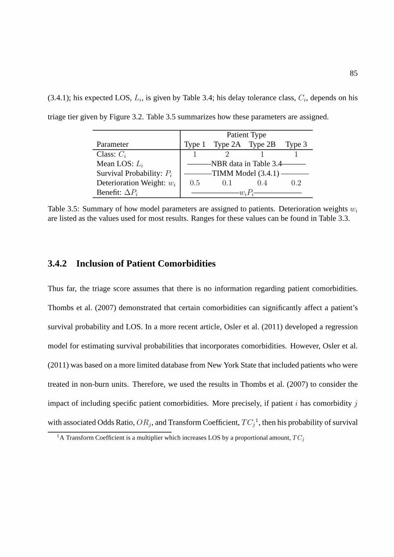
85

(3.4.1); his expected LOS,Li, is given by Table 3.4; his delay tolerance class,Ci, depends on his

triage tier given by Figure 3.2. Table 3.5 summarizes how these parameters are assigned.

Patient TypeParameter Type 1 Type 2A Type 2B Type 3Class:Ci 1 2 1 1Mean LOS:Li ———NBR data in Table 3.4———Survival Probability:Pi ———–TIMM Model (3.4.1) ———–Deterioration Weight:wi 0.5 0.1 0.4 0.2Benefit:∆Pi ——————wiPi——————

Table 3.5: Summary of how model parameters are assigned to patients. Deterioration weightswi

are listed as the values used for most results. Ranges for these values can be found in Table 3.3.

3.4.2 Inclusion of Patient Comorbidities

Thus far, the triage score assumes that there is no information regarding patient comorbidities.

Thombs et al. (2007) demonstrated that certain comorbidities can significantly affect a patient’s

survival probability and LOS. In a more recent article, Osler et al. (2011) developed a regression

model for estimating survival probabilities that incorporates comorbidities. However, Osler et al.

(2011) was based on a more limited database from New York State that included patients who were

treated in non-burn units. Therefore, we used the results inThombs et al. (2007) to consider the

impact of including specific patient comorbidities. More precisely, if patienti has comorbidityj

with associated Odds Ratio,ORj, and Transform Coefficient,TCj1, then his probability of survival

1A Transform Coefficient is a multiplier which increases LOS by a proportional amount,TCj

86

and LOS are adjusted from the base values if he did not have thecomorbidities:

P Yi =

PNi

PNi + (1− PN

i )ORj

LYi = TCjL

Ni (3.4.2)

where the superscript denotes whether the patient has the comorbidity: Y for Yes, andN for No.

Note that the TIMM model and LOS estimates include patients with comorbidities. Hence, those

estimates can be used to determinePNi andLN

i based on the prevalence,qj , of comorbidityj in

the sample used for estimation:

E[Pi] = (1− qj)PNi + qjP

Yi = (1− qj)P

Ni + qj

PNi

PNi + (1− PN

i )ORj

E[Li] = (1− qj)LNi + qjL

Yi = (1− qj)L

Ni + qjTCjL

Ni (3.4.3)

Table 3.6 summarizes the Odds Ratios and Transform Coefficients for the comorbidities which

have statistically significant impact on mortality and/or LOS. It also includes the prevalence in the

National Burn Repository dataset which was used to estimatethese parameters and was required

to determinePNi andLN

i .

Thombs et al. (2007) determined that if a patient has more than one comorbidity, then his

survival probability is first adjusted by the most significant (in terms of impact) comorbidity, and

is further adjusted by each additional (but no more than three) comorbidities using an odds ratio

of 1.33. For example, consider a 50 year old patient with TBSA= 11% and no inhalation injury;

hence, he is Type 2A. This patient has renal disease and is obese. Based on his age, TBSA, and

87

Prevalence (%)Co-morbidity Category OR TC NBR NYC USHIV/AIDS 10.19 1.49 0.2 0.46 0.37Renal Disease 5.11 1.44 0.6 16.8Liver Disease 4.82 1.3 0.6 2Metastatic Cancer 4.55 NS 0.6 0.447Pulmonary Circulation Disorders2.88 NS 0.1 <3Congestive Heart Failure 2.39 1.23 1.6 1.76Obesity 2.11 NS 1.2 25.6 33.8Malignancy w/o Metastasis 2.08 NS 0.4 0.447Peripheral Vascular Disorders 1.84 1.39 0.6 5|50+Alcohol Abuse 1.83 1.36 5.8 4.65 4.3Other Neurological Disorders 1.56 1.52 1.6 <2Cardiac Arrhythmias 1.49 1.4 2.0 12.6|60+Cerebrovascular Disease NS 1.14 0.3 <2Dementia NS 1.6 0.3 13.9|70+Diabetes NS 1.26 4.4 12.5 7.8Drug Abuse NS 1.2 3.3 16 14Hypertension NS 1.17 9.6 28.8 21.7Paralysis NS 1.9 1.7 1.9Peptic Ulcer Disease NS 1.53 0.4 <1Psychiatric Diagnosis NS 1.42 2.9 <1Valvular Disease NS 1.32 0.4 <2

Table 3.6: Odds Ratio (OR), Transform Coefficient (TC), and prevalence of various Comorbiditiesas reported in Thombs et al. (2007) and others. Prevalence isgiven for the American Burn Asso-ciate National Burn Repository (ABA-NBR), while for New York City and the United States, itis given for the general population. When it is specified by age, the age group is listed after theseparation bar, i.e. the prevalence for Peripheral Vascular Disorder is given for people aged 50 andolder.

lack of inhalation injury, his nominal survival probability and expected LOS arePNi = .918 and

LNi = 13.6 days. His deterioration factor isw2A = 0.1. Now, we adjust for the comorbidities:

first adjusting for renal disease and then adjusting with an odds ratio of 1.33 for additionally being

88

obese:

P Yi =

PNi

PNi +(1−PN

i )5.11

PNi

PNi +(1−PN

i )5.11+ (1− PN

i

PNi +(1−PN

i )5.11)1.33

= .622

LYi = 1.44LN

i = 19.6 days (3.4.4)

We can see that this patient’s comorbidities significantly alters his triage priority index from

∆Pie3/Li = 0.1145 to ∆PA

i e3/LA

i = .07249. Depending on the demographics of the other pa-

tients, this change could be the difference between being transferred first or last.

3.4.3 Summary of Proposed Triage Algorithm

The triage algorithm can be summarized as follows:

1. For each patient,i, determine his triage type, survivability,PAi , and expected LOS,LA

i . The

superscriptA denotes the fact that these parameters are adjusted if it is known the patient

has or does not have a significant comorbidity.

2. Patienti’s benefit is∆Pi = wiPAi ; his deterioration factorwi = 0.5 if patient i is Type 1,

wi = 0.1 if he is Type 2A,wi = 0.4 if he is Type 2B, andwi = 0.2 is he is Type 3; his class

isCi = 2 if patienti is Type 2A, otherwiseCi = 1.

3. Prioritize patients based on their triage index:∆Pie3/LA

i

4. Patienti generates reward∆Pi[1ti≤3,Ci=1 + 1ti≤5,Ci=2], whereti is the time at which he

is transferred into a Tier 1 burn bed.

89

Note that the presented algorithm serves as the baseline forpatient prioritization and clinical

judgment can be used to reduce a patient’s prioritization inspecial circumstances such as family

wishes for limited end of life care, presence of a imminentlyterminal illness, and/or a Glasgow

Coma Score of less than 6, which reflects severe brain injury low cognitive activity.

3.5 Evaluating the Algorithm

We now evaluate our proposed algorithm relative to four others using simulation. The first algo-

rithm, referred to as the Original Algorithm, is the original three tier triage matrix proposed in Yurt

et al. (2008) and depicted in Figure 3.2. Because there is no differentiation within each tier, the

algorithm is equivalent to randomly prioritizing patientswithin each tier. The second algorithm,

referred to as the Survival Algorithm, follows the initial proposal of the Task Force which is to

differentiate patients within a single triage tier based only on survival probability. The remaining

algorithms utilize the parameters whose estimation is given in Section 3.4.1. The third algorithm is

Weighted Shortest Processing Time First. The fourth algorithm, refereed to as the Proposed-N al-

gorithm is our proposed algorithm but assumes noinformation about comorbidities is known. The

fifth algorithm is our Proposed-W algorithm withcomorbidities, i.e. it accounts for the presence

(or lack) of comorbidities and ranks patients based on theiradjustedindex. We use simulation to

estimate expected rewards. Details of our simulation modelcan be found in the Appendix. Table

3.7 summarizes the algorithms which are simulated.

90

Triage Algorithm IndexOriginal (from Yurt et al. (2008)) Tiered with Random SelectionSurvival Tiered with priority in each tier according to:Pi

WSPT ∆Pi/LAi

Proposed-N ∆Pie3/Li

Proposed-W ∆Pie3/LA

i

Table 3.7: Triage Index. Higher index corresponds to higherpriority for a Tier 1 bed.

3.5.1 Data Description

In this section we describe the patient data which we use in our simulation model to compare the

triage algorithms described in the previous section. We have a number of data sources: 775 cases

of patients treated at the New York-Presbyterian/Weill Cornell Medical Center Burn Center during

the year 2009, published data from previous disaster eventsand published census data. The patient

population from NY Presbyterian (NYP) is generally not indicative of what would be expected in

a disaster scenario–for example, nearly 50% of the patientsare under the age of 5 and the median

TBSA was 2%. Given that age is a significant factor in determining patient survivability and LOS,

we turn to published data on previous disaster events to build representative scenarios of the types

the Federal Health Resources and Services Administration wants to prepare for. We will return to

the NYP data when considering the feasibility of the federalmandate in Section 3.6.

Each simulation scenario we consider attempts to emulate the demographics and severity of

prior burn disasters. We looked at four disaster events: theWorld Trade Center attacks on Septem-

ber 11, 2001 in NYC (Yurt et al. 2005), a 2002 suicide bombing in Bali (Chim et al. 2007), a

2003 suicide bombing at the Jakarta Marriot hotel (Chim et al. 2007), and a 2003 nightclub fire in

Rhode Island (Mahoney et al. 2005). The patients’ ages rangefrom 18 to 59 and the severity of

burns range from 2% to 100% TBSA. These statistics are summarized in Table 3.8. The patients

91

in the four disaster events were older and experienced more severe burns than the average patient

treated at NYP in 2009.

Age TBSA IHIEvent Median Min. Max. Median Min. Max.NYC 9/11 2001 44 (avg.) 27 59 52% (avg.) 14% 100% 66.7%Bali 2002 29 20 50 29% 5% 55%Jakarta 2003 35 24 56 10% 2% 46%Rhode Island 2005 31 (avg.) 18 43 <20% <20% >40%

Table 3.8: Distribution of age, severity of burn (TBSA), andinhalation injury (when known) inburn data as summarized from Yurt et al. (2005), Chim et al. (2007), Mahoney et al. (2005).

Outside of the NYC 9/11 2001 event, there was no information on patient inhalation injury.

However, the data from the National Burn Repository (NBR) does include this information for

burn-injured patients treated from 1973-2007. We have summarized the distribution of IHI based

on age and extent of burn in Table B.1 in the Appendiz. The average IHI across patients in the

NBR data who fall within the same demographics as NYC 9/11, i.e. age from[30, 60] and TBSA

from [20%, 100%], is 48.95%, which is slightly lower than the observed 66.7% documented from

9/11.

There was no information on the presence of comorbidities inthese references. We used a

series of references to collect prevalence data of relevantcomorbidities in the general population.

Prevalence of any given comorbidity could be dependent on the type of event as well as where it

takes place. The population in an office building may have a different set of demographics than that

in a subway or sports arena. Therefore, it would be desirableto have prevalence data based on, at

the very least, age and gender. However, this fine-grained information was not generally available

and so, for consistency, we used prevalence for the general population. In some cases, we were

able to get prevalence data specific to NYC or New York State rather than national data. Since

92

these data more closely correspond to the potential burn-injured patient population for which the

algorithm was being developed, we used these when available. The prevalence of the comorbidities

of interest are summarized in Table 3.6.

3.5.2 Simulation Scenarios

Due to the variability across the burn disaster events, we consider a number of simulation scenarios.

We simulate the average increase in number of survivors due to Tier 1 treatment for the triage

policies described above.

For the sake of simplicity, our simulations assume that all burn beds are available to handle

the burn victims resulting from the catastrophe. We discussthe implications of this assumption

later. The number of burn beds is fixed at 210 to represent the total number of Tier 1 beds in the

NYC region when accounting for the surge capacity. We consider scenarios which are likely to be

representative of an actual burn disaster. The first scenario is based on the Indonesia and Rhode

Island events. Age is uniformly distributed from[18, 60], burn severity is uniformly distributed

from [0%, 60%], and inhalation injury is present with probability which isconsistent with 9/11, i.e.

.667. For our second scenario, we consider inhalation injury which is dependent on age and TBSA

as summarized in Table B.1. Our third and fourth scenarios aim to be representative of events like

NYC 9/11: the age distribution is still[18, 60], but the extend of the burn is more severe with TBSA

uniformly distributed from[10%, 90%]. In summary, the four scenarios we consider are listed in

Table 3.9, and Table 3.10 shows the statistics of patients interms of class and Type under each

scenario.

93

Age TBSA IHIScenario Uniform Distribution Uniform Distribution Bernoulli Distribution1 [18, 60] [0%, 60%] .6672 [18, 60] [0%, 60%] NBR Data in Table B.13 [18, 60] [10%, 90%] .6674 [18, 60] [10%, 90%] NBR Data in Table B.1

Table 3.9: Distribution of age, severity of burn (TBSA), andinhalation injury for four simulationscenarios.

Scenario Class 1 Class 2 Type 1 Type 2 or 31 93.9% 6.1% 85.5% 14.4%2 81.7% 18.3% 74.2% 25.8%3 95.9% 4.1% 58.7% 41.3%4 88.8% 11.3% 54.5% 45.4%

Table 3.10: Scenario Statistics

3.5.3 Simulation Results: Unknown Comorbidities

We compare the relative improvement in benefit under four different triage algorithms described

in Table 3.7. Hence, the performance is given by the increasein average number of survivors due

to timely transfer into Tier 1 beds within the 3-5 day window divided by the number of survivors

under the original block triage system. We assume that comorbidities are unknown or ignored.

Hence, in this casePAi = Pi andLA

i = Li, so that the Proposed-N and Proposed-W algorithms

are identical. Figure 3.3 shows the relative improvement ofthe objective compared to the original

triage algorithm from Yurt et al. (2008).

It is clear that the impact of including LOS in the triage score depends on the type of event as

given by the age and severity of the burn victims. In severe cases (Scenario 3 and 4), ignoring LOS

and simply using survivability (Survival Algorithm:P0) does noticeably worse than the Proposed-

N algorithm. The Proposed-N algorithmalwaysoutperforms the original algorithm, by as much as

94

200 250 300 350 400−0.05

0

0.05

0.1

# of patients

Rel

ativ

e im

prov

emen

t

Improvement in the objective, Scenario 1

200 250 300 350 400−0.05

0

0.05

0.1

# of patients

Rel

ativ

e im

prov

emen

t


200 250 300 350 400−0.05

0

0.05

0.1

# of patients

Rel

ativ

e im

prov

emen

t


200 250 300 350 400−0.05

0

0.05

0.1

# of patients

Rel

ativ

e im

prov

emen

t


P0WSPTProposed−N

Figure 3.3: Relative Improvement of Average Additional Survivors

10%, which corresponds to 21 additional lives saved. In somecases, WSPT generates more than

5% less benefit than the original algorithm; this is expectedas discussed in Section 3.3.1, WSPT

is suboptimal.

3.5.4 Simulation Results: Comorbidities

We now consider the impact of incorporating comorbidities in triaging patients. Determining the

presence of comorbidities may be costly or difficult. This determination has to be made within the

first hours, and certainly within the first day as triage decisions are made. Some comorbidities,

such as obesity, can easily be determined upon simple examination while others, such as HIV

may be less so. Though some comorbidities will show up via routine blood work done upon

95

arrival to the hospital, the laboratory may be overwhelmed in a disaster scenario, causing delays

in obtaining these results. Additionally, some patients may arrive to the hospital unconscious or

they may be intubated immediately upon arrival to the hospital making it difficult or impossible

for them to communicate which comorbidities they have. As information about comorbidities

becomes available, they can be used to transfer patients to the correct tier.

The NYC Task Force was hesitant to incorporate comorbidities into the triage algorithm due

to potential difficulties in identifying the presence of comorbidities. However, as seen in Thombs

et al. (2007), the presence of comorbidities can significantly affect mortality and LOS, which will

ultimately affect a patient’s triage priority. Uncertainty about the presence of a comorbidity may

result in an incorrect triage priority, ultimately resulting in a reduction in total average benefit

generated by the triage algorithm. On the other hand, the impact of some comorbidities may be so

limited that knowledge of them would not significantly affect the expected benefit. Therefore, it is

important to determine which comorbidities are likely to beworth the cost of identifying for use

in triage.

For each comorbidity,j, with associated Odds Ratio,ORj, Transform Coefficient,TCj, and

prevalence,qj , consider the following two extreme scenarios:

1. Perfect information of comorbidityj is available. That is, we know whether each patient

does or does not have comorbidityj, in which case we can adjust the survival probability

and LOS accordingly as described in (3.4.2). That is, if the patient has the comorbidity,

PAi = P Y

i andLAi = LY

i , elsePAi = PN

i andLAi = LN

i .

2. No information of comorbidityj is available. We assume each patient has comorbidityj

96

with probability qj, whereqj is the prevalence of comorbidityj in the population. The

expectation of the adjusted probability and probability ofcompleting within 3 days are:

PAi = qjP

Yi + (1− qj)P

Ni

E[P (Si < 3)] = E[e3/LAi ] = qje

3/LYi + (1− qj)e

3/LNi (3.5.1)

wherePNi andLN

i are the nominal survival probability and LOS, respectively, given patient

i has no comorbidities. Patienti’s index is then given by∆PiE[e3/LA

i ], with ∆Pi = wiPAi .

For each comorbidity, we compare the average additional number of survivors due to burn bed

treatment in each scenario. In particular, we examine the relative improvement of having perfect

information for comorbidityj versus having no information. Again, we consider the four scenarios

based on the previous disaster events. Because these references do not have information regard-

ing comorbidities, we randomly generated comorbidities for each patient based on the available

prevalence data in Table 3.6. We generated 10,000 patient cohorts and corresponding realizations

of LOS, survival, inhalation injury, and (non)existence ofcomorbidityj.

The comorbidities with significant impact are summarized inTable 3.11. The comorbidities

which are omitted have no significant impact due to small effect on LOS or survival and/or due

to low prevalence. In all scenarios, renal disease has the most significant improvement for having

full information versus no information with relative improvement 1.381%-1.578%. The relative

improvement for all remaining comorbidities is less than 0.5%–more than a factor of 2 less than

renal disease. We note that in this case, renal disease includes varying levels of disease severity

and is defined by 13 different ICD9 codes, one of which corresponds to end stage renal disease.

97

Relative Improvement (Std Err)Comorbidity Category Scenario 1 Scenario 2 Scenario 3 Scenario 4Renal Disease 1.534 ( 0.036 ) 1.486 ( 0.038 ) 1.578 ( 0.043 ) 1.381 ( 0.040 )Obesity 0.332 ( 0.029 ) 0.356 ( 0.030 ) 0.402 ( 0.033 ) 0.332 ( 0.033 )Liver Disease 0.288 ( 0.017 ) 0.313 ( 0.018 ) 0.335 ( 0.020 ) 0.277 ( 0.018 )HIV/AIDS 0.119 ( 0.008 ) 0.108 ( 0.009 ) 0.109 ( 0.010 ) 0.090 ( 0.009 )Pulmonary Circ. Disorder 0.101 ( 0.013 ) 0.108 ( 0.014 ) 0.134 ( 0.016 ) 0.117 ( 0.015 )Alcohol Abuse 0.087 ( 0.013 ) 0.095 ( 0.014 ) 0.109 ( 0.016 ) 0.082 ( 0.015 )Congestive Heart Failure 0.074 ( 0.010 ) 0.061 ( 0.011 ) 0.071 ( 0.012 ) 0.047 ( 0.011 )Metastatic Cancer 0.045 ( 0.007 ) 0.033 ( 0.007 ) 0.052 ( 0.008 ) 0.047 ( 0.007 )Peripheral Vasc. Disorder 0.028 ( 0.007 ) 0.025 ( 0.007 ) 0.031 ( 0.008 ) 0.041 ( 0.007 )

Table 3.11: Impact of comorbidity information: Relative improvement and standard error in per-centages.

Recognizing highly complex algorithms which require a lot of information gathering and training

will be difficult to implement during disaster scenarios, weelect to include only one comorbidity

in the final triage algorithm: renal disease.

3.5.5 Performance of the Proposed Triage Algorithm

The final triage algorithm we propose prioritizes patients based on the index which is the ratio

of their benefit in probability of survival from treatment ina burn bed to their adjusted probabil-

ity of completing treatment within 3 days:∆PAi e

3/LAi . A patient’s LOS and benefit are adjusted

if the patient has renal disease, but ignores all other comorbidities. In our simulations, we as-

sume full knowledge of renal disease since this may be detected through routine blood tests2. In

more extreme cases of renal disease, such as chronic, end stage renal disease requiring dialysis, a

physical exam that reveals an implanted dialysis catheter can reveal such a condition. Using our

simulation model described in the Appendix, we compare the performance in terms of average

2We note that other insults to the renal system that may resultfrom acute burn trauma or resuscitation process canmimic these findings.

98

increase in number of survivors due to burn bed treatment of the Proposed-W triage algorithm to

the Proposed-N algorithm (Figure 3.4) and to the original one which was proposed in Yurt et al.

(2008) (Figure 3.5) which do not utilize comorbidity information to adjust a patient’s probability of

survival and expected LOS. In all scenarios, the Proposed-Walgorithm achieves over 1.5% more

reward (3 additional lives saved) than the Proposed-N algorithm and 2.5% more reward than the

original algorithm. In Scenario 1, Proposed-W achieves up to 15% more reward (31 additional

lives saved).

250 300 350 4000

0.005

0.01

0.015

0.02

# of patients

Rel

ativ

e im

prov

emen

t


Proposed−W vs.Proposed−N

250 300 350 4000

0.005

0.01

0.015

0.02

# of patients

Rel

ativ

e im

prov

emen

t


250 300 350 4000

0.005

0.01

0.015

0.02

# of patients

Rel

ativ

e im

prov

emen

t


250 300 350 4000

0.005

0.01

0.015

0.02

# of patients

Rel

ativ

e im

prov

emen

t


Figure 3.4: Relative Improvement of Average Increase in Number of Survivors due to Tier 1treatment: Proposed-W versus Proposed-N

Under severe disaster scenarios (Scenarios 3 and 4), the relative benefit is much lower. This

is because in severe events, the number of survivors is goingto be quite low, irrespective of the

99

250 300 350 4000

0.05

0.1

0.15

# of patients

Rel

ativ

e im

prov

emen

tImprovement in the objective, Scenario 1

Proposed−W vs. by Tier

250 300 350 4000

0.05

0.1

0.15

# of patients

Rel

ativ

e im

prov

emen

t


250 300 350 4000

0.05

0.1

# of patients

Rel

ativ

e im

prov

emen

t


250 300 350 4000

0.05

0.1

# of patients

Rel

ativ

e im

prov

emen

t


Figure 3.5: Relative Improvement of Average Increase in Number of Survivors due to Tier 1treatment: Proposed-W versus Original

algorithm used. Additionally, there is low bed turnover (only 7-12 additional patients are admitted

from the Tier 2/3 hospitals within 3-5 days as compared to up to 36 additional patients under

Scenario 1), so all algorithms are unable to provide treatment in burn units for many patients

beyond the initial 210 which are admitted. However, we note that in such cases, accounting for

LOS is even more essential because any sort of turnover will be helpful (refer back to Figure 3.3

to see the benefits of including LOS). While prioritizing solely based on survivability performs

reasonably well, we emphasize that the Proposed-W algorithm still outperforms the others.

It is also interesting to consider the variation in the number of survivors under each triage

algorithm. While we notice that the Proposed-W policy out performs all other policies with respect

100

to expected number of survivors, this could potentially come with increased variation, i.e. risk.

When comparing the standard deviation of the number of survivors in our simulations, we find

that the Proposed-W policy always has the smallest standarddeviation. Hence, we find that our

proposed algorithm not only yields a higher expected numberof survivors, but also a slightly lower

level of uncertainty.

We note that the results were similar over various values of the deterioration factors within the

allowable ranges specified in Table 3.3. In all cases, Proposed-W outperformed all of the other

policies. The magnitude of this improvement varied from 2.2%-16.1%.

3.6 Feasibility

In this section, we analyze the feasibility of admitting alleligible burn-injured patients to a burn

center during the specified time frame during a catastrophe given the current burn bed capacity and

the proposed burn disaster plan. With a surge capacity of 210burn beds in the NYC region, all

patients can be immediately cared for in a Tier 1 bed if there are 210 or fewer patients. However,

as can be seen in Table 3.4, burn-injured patients can have long recovery times–much longer than

5 days–and so it is not at all clear that the requisite 400 patients can all be transferred to a burn bed

during the 3-5 day time period.

The feasibility of meeting the government mandate will be highly dependent on the size of the

event, i.e. the number of patients, as well as the severity ofthe patients. If most patients have

minimal burns (i.e. TBSA< 10%), they will have shorter LOS; there will be more turnoverin

the Tier 1 burn beds; and more patients can be cared for in the first few days following the event.

101

On the other hand, if most patients have very severe burns, they will have very long LOS and it is

unlikely that many new patients will be transferred within the specified time frame.

We consider the four scenarios for events as summarized in Table 3.9. The number of Tier 1

beds is fixed at 210 and we vary the number of patients in the event. For all of our simulations, we

use the Proposed-W triage algorithm which includes information about renal disease and prioritizes

patients according to their score:∆Pie3/LA

i . Figure 3.6 shows the percentage of admitted patients.

With more than 250 patients, some patients cannot be transferred within the specified 3-5 day

window. In events with more severe patients (Scenario 3 and 4), more than 45% of the 400 patients

cannot be transferred within the desired time frame.

200 250 300 350 4000.5

0.6

0.7

0.8

0.9

1

# of patients

frac

tion

of p

atie

nts

adm

itted

fraction of patients admitted, Scenario 1

Proposed

200 250 300 350 4000.5

0.6

0.7

0.8

0.9

1

# of patients

frac

tion

of p

atie

nts

adm

itted


200 250 300 350 4000.5

0.6

0.7

0.8

0.9

1

# of patients

frac

tion

of p

atie

nts

adm

itted


200 250 300 350 4000.5

0.6

0.7

0.8

0.9

1

# of patients

frac

tion

of p

atie

nts

adm

itted


Figure 3.6: Feasibility: Number of beds fixed at 210

102

3.6.1 Clearing Current Patients

In assessing the feasibility of meeting the government mandate, we assumed that the burn centers

could be cleared of all current patients in order to accommodate new patients from the burn disaster.

On September 11, 2001, New York Presbyterian (NYP) was able to transfer all current patients to

make room for all new burn-injured patients (Yurt et al. 2005). However, there were only 41 burn-

injured patients who were directly admitted or transferredinto a burn center, which is substantially

smaller than the 400 required by the federal government.

New York Presbyterian (NYP) has one of the largest burn centers in the country with 40 beds.

We obtained data on all patients who were treated in this center during 2009 including patient

age, burn severity as measured by TBSA, presence of inhalation injury, gender, length-of-stay, and

comorbidity information. While the patient population andseverity of these 775 patients is quite

different than prior burn disasters, we can utilize this data to consider the likelihood of clearing all

patients if a disaster occurs.

In 2009, the average daily arrival rate was 2.12 per day with astandard deviation 1.56. Daily

arrivals ranged from 0 to 7. Figure B.1 in the Appendix shows the monthly and day-of-week

patterns of daily arrivals. There was a peak in arrivals fromJanuary-April, which is consistent

with anecdotal evidence from the burn clinicians, since burns are much more common in the winter

months. Differences in arrival rate across days of the week are not significant, though the number

of admissions on Tuesdays is slightly higher. More importantly, the burn specialists at the NYP

burn center estimate that the burn center is overcrowded on the order of twice a week during winter

months. Hence, the number of beds which are available to carefor burn disaster patients is likely

103

to vary significantly depending on when the event takes place. Some current patients may be too

severely injured to move out of the burn center, effectivelyremoving beds from the disaster plan.

The assumption of being able to clear all current patients ishighly optimistic, making the feasibility

of transferring all patients even more unlikely.

Given the possibility of having fewer than the maximum 210 beds, we consider how much more

difficult it is to satisfy the federal mandate when fewer bedsare available. Specifically, we assume

there are 400 burn-injured patients, as given by the federalmandate and consider the percentage of

patients who are admitted within their deadline of 3 or 5 days, as appropriate. As seen in Figure

3.7, for a wide range of scenarios, it is likely that fewer than 200 patients (i.e.< 50%) will be able

to receive Tier 1 care within the desired time frame.

50 100 150 2000

0.1

0.2

0.3

0.4

0.5

0.6

0.7

# of beds

frac

tion

of p

atie

nts

adm

itted


Proposed

50 100 150 2000

0.1

0.2

0.3

0.4

0.5

0.6

0.7

# of beds

frac

tion

of p

atie

nts

adm

itted


50 100 150 2000

0.1

0.2

0.3

0.4

0.5

0.6

0.7

# of beds

frac

tion

of p

atie

nts

adm

itted


50 100 150 2000

0.1

0.2

0.3

0.4

0.5

0.6

0.7

# of beds

frac

tion

of p

atie

nts

adm

itted


Figure 3.7: Feasibility: Number of patients fixed at 400

104

Clearly, the NYC disaster plan cannot meet the guidelines ofthe Federal Health Resources

and Services Administration. In order to treat 50 burn-injured patients per million in population

in NYC, more resources would be needed. Either more actual burn beds with the corresponding

surgical facilities and professional staff capabilities would need to be provided or federal support to

transport patients to burn centers in other states would be necessary to care for all 400 burn-injured

patients. The amount of additional resources needed would vary depending on the type and size of

event.

3.7 Conclusions and Discussion

Hospital systems and governments must be prepared to handlepotential disaster events where the

number of patients who seek care exceeds the initial available resources. Federal guidelines specify

that metropolitan areas be able to care for 50 burn-injured patients per million in the 3 to 5 days

following such an event. In this study, we presented a triagesystem to maximize the expected

benefit and applied it to evaluate the feasibility of meetingthis standard given the mix of burn and

non-burn trauma beds that have been designated for use during a burn disaster in New York City.

This triage algorithm is the first to incorporate burn centerLOS and comorbidities to prioritize

patients for transfer to burn beds.

Given the initial proposed NYC disaster plan, which utilizes burn beds in NYC and hospitals

within a 60-mile radius region which have agreed to assist inan event, it is highly unlikely that

all burn-injured patients will be able to be transferred into a Tier 1 burn bed within 5 days. More-

over, ignoring patient LOS and some comorbidities would additionally reduce the total benefit to

105

treated patients. These findings persuaded the NYC Task Force to incorporate these factors into

their proposed revised triage plan. Leahy et al. (2011) describes the current burn disaster plan rec-

ommendation by the NYC Task Force, including the triage plandescribed here, in addition to other

considerations such as medical training for EMS and Tier 2/3personnel and provider indemnity.

While we focus on burn disaster planning in NYC, the insightsgained from this work can

be applied to other cities. Because NY is the largest city in the United States, it is often seen

as a model for other metropolitan areas. In particular, it isclear that any triage system should

incorporate LOS and some comorbidities such as renal disease. The need to explore methods

to expand resources in order to satisfy the federal mandate depends on the current burn center

resources and population. Certainly, NY has the largest patient requirement, but it also has one of

the largest (if not largest) aggregate number of burn beds. There are only 125 burn centers in the

United States (American Burn Association 2009), so while there are 9 burn centers within a 60

mile radius of NYC, other cities may be more limited in the number of beds available at nearby

burn centers. In situations where burn centers are available, these smaller cities are likely to be

even more capacity constrained than NYC, making it even moreessential to utilize a carefully

designed triage algorithm.

One limitation of this work is that all of the available LOS data is based on scenarios where

there is not a large backlog of patients waiting to be transferred into the burn center. Furthermore,

the LOS from Saffle et al. (2005) ishospitalLOS, not burn center LOS. However, these can be

considered equivalent since most burn-injured patients are discharged directly from the burn center.

In a catastrophic scenario, it may be possible to transfer burn-injured patients to non-burn beds

before they are ready to be discharged from the hospital. This could free burn beds earlier, enabling

106

additional patients to receive the necessary skin graftingsurgeries or wound care thereby increasing

the number of patients who are able to benefit from care in Tier1 beds. There is no available data

regarding what theminimal LOS in the burn center would be; hence, we could not accurately

account for this in our model. It may be possible to reduce LOS–a Canadian burn center was

able to reduce patient LOS for patients with TBSA less than 20% and who did not require surgery

(Jansen et al. 2012). However, the majority of patients in the disaster scenario considered in this

study are likely to require surgery and/or have TBSA greaterthan 20%, so it is not clear whether

any significant reduction in LOS could be achieved in this situation. Another limitation is that we

have inferred the benefit of receiving treatment in a burn center within 3-5 days from the existing

burn triage matrix. There is currently no quantitative dataon the outcomes (survival or LOS) of

burn-injured patients who are not treated in specialized burn centers nor is there any evidence-based

model of the impact of delay of surgery on mortality for patients in the first few days after injury.

The only available information is qualitative and minimal,i.e. more sophisticated treatments which

are often performed in burn centers has significantly improved LOS (Curreri et al. 1980), or based

on clinical judgement as in Yurt et al. (2008). However, as more data becomes available, our

methodology can be modified appropriately.

Finally, our triage model, as any other triage model, assumes accurate knowledge of the burn

size and severity of each patient. Yet, anecdotal evidence (e.g. Lozano (2012)) suggests that

non-burn physicians often misjudge the extent of burns resulting in both overestimates and un-

derestimates. One possible remedy is the installation of high-resolution cameras in the Tier 2/3

hospitals that would enable burn specialist to make the assessments of TBSA for triage purposes.

Such a program was successfully instituted at Lehigh ValleyHealth Network, Pennsylvania.

107

Despite these limitations, our work has improved upon the burn disaster plan initially devel-

oped by the NYC Task Force and described in Yurt et al. (2008).In particular, our proposed triage

algorithm, which incorporates a continuous model for survival likelihood, patient LOS, and co-

morbidities, increases the number of survivors due to Tier 1treatment by up to 15%. Perhaps the

most practically useful insight from this study is that the proposed tiered system may be sufficient

in small to moderately sized events; however, the current resources are likely to be insufficient

when the number of patients is large and/or the severity of burns is high. More generally, this

demonstrates that non-burn beds that are used to stabilize patients awaiting care in a burn center

have limited usefulness due to the long LOS of severely burned patients.

108

Chapter 4

The Design of Service Delivery Systems with

Workload-dependent Service Rates

4.1 Introduction

In this research, we focus on analyzing the productivity of aservice delivery system (SDS) as char-

acterized by the service rate of its server – trained employees which constitute the main resources

to handle the incoming service requests to the system. Our objective is to identify different mech-

anisms by which the design of the request allocation policy can influence the productivity of its

employees, which can then be used to improve the SDS design tomaximize its efficiency.

We look at a typical SDS under which resources are managed centrally. The SDS consists of

a number of “agents”, and is responsible for handling service requests (“requests”) brought up by

its customers. A dispatcher receives the requests and assigns them to agents following established

processing standards. The service delivery process involves two stages. The dispatcher first decides

109

when and to which agent each request is assigned, and then each agent independently controls the

order in which he processes the requests that have been assigned to him.

In order to identify desirable features of the request allocation and workload management pol-

icy for the dispatcher, we study the link between request allocation policies and the performance of

the SDS. A key aspect affecting the system performance is theagents’ service rates. While tradi-

tional queuing models of SDS’s typically consider the service rate to be constant, recent empirical

work suggests that an agent’s service rate can be influenced by the system workload (KC and

Terwiesch (2009), Schultz et al. (1999, 1998)). Consequently, the dispatcher can impact agents’

service rates by managing each agent’s workload, which contains all the requests assigned to that

agent, and thereby affect the SDS’s performance.

We conduct our empirical analysis based on data collected from a world leading IT service

delivery provider with globally distributed service delivery centers. A novel dataset, which tracks

the detailed time intervals each agent spends on all business related activities, is collected for the

special purpose of studying the agent’s behavior in managing his workload. Using this detailed

data, we develop a novel methodology, based on econometric techniques from survival analysis, to

study productivity. The resulting measure can be interpreted as the agent’s instantaneous service

rate at which he processes requests. Our approach enables usto identify different mechanisms by

which workload affects productivity, which is challengingto measure using traditional productivity

measures such as throughput rates and service times. The identification of these mechanisms

provides interesting insights for the design of the workload allocation policy.

Specifically, we seek to explore the following four distinctive mechanisms by which workload

affects productivity. In the first mechanism, which resembles the optimal control of queues with

110

dynamic adjustments of the service rate (George and Harrison (2001)), higher workload levels

may cause agents to temporarily increase their service rate(possibly incurring higher cognitive

costs) to reduce the waiting time of the requests in his workload. (KC and Terwiesch (2009)

identify such an effect in patient transport of a hospital.)In the second mechanism, workload

generates work accumulation that may affect productivity through learning-by-doing (Pisano et al.

(2001)) and fatigue/stress (Kuntz et al. (2012)). In the third mechanism, higher workload may

result in the occurrence of longer or more frequent interruptions, which may break the agent’s

working rhythm and generate a negative impact on productivity (Schultz et al. (2003)). In the fourth

mechanism, higher workload provides agents with more flexibility to arrange the order in which

they process requests, potentially taking advantage of such flexibility to improve productivity. In

particular, agents may learn from specialization and become more productive when focusing on

similar requests (Staats and Gino (2012)).

The identification of these mechanisms has different insights for the request allocation policy.

First, we find that the agent’s speed of work increases with his individual workload level, but the

marginal increase in productivity diminishes as the workload increases. In contrast, the workload

of the entire team does not have a significant impact on agents’ productivity. These findings suggest

that the dispatcher has the incentive to assign requests to an agent earlier in order to keep individual

workload at a high level to increase his productivity. Second, we find that agents’ productivity also

increases with accumulated workload during the working shift, demonstrating a learning-by-doing

effect. Third, we find that different types of interruptionshave different temporary impacts on

agent productivity. This implies the cost of having higher workload levels, because higher work-

load levels may result in longer suspending periods once a request is interrupted, which require

111

additional set-up efforts when agents revisit the requests. Finally, we find that short-term special-

ization boosts productivity as agents become more productive when working on similar requests,

suggesting that it may be beneficial to assign similar requests to each agent.

Based on these findings, we further explore managerial insights regarding the request allocation

policies by analyzing a team that serves requests of two priory levels. Each priority level has an as-

sociated service level agreement (“SLA”) which specifies its contractually required level of service

performance as measured by the request completion time. We compare the team performance in

terms of the minimal number of agents required to meet the SLAs associated with the two priority

levels under three commonly used request allocation policies: (i) thedecentralized system, where

the dispatcher does not hold any requests and assigns each request to an agent upon arrival; (ii)

thecentralized system, where the dispatcher holds a central queue of requests and assigns requests

as agents become available; (iii) thestream system, where agents are separated into two groups to

independently handle two priority levels of requests.

After accounting for agents’ behavior of managing their processing order, our empirical find-

ings imply the following trade-off among these three systems. The decentralized system takes full

advantage of the productivity boost by keeping all the requests in agents’ workload. The central-

ized system enjoys the benefit of resource pooling and centralized control, because the dispatcher

can fully manage the processing order of different requeststo ensure that different requests are effi-

ciently prioritized to meet SLA requirements. However, thecentralized system suffers from lower

productivity since all the requests are kept as the team’s workload rather than the agent’s individual

workload. The stream system combines some features from each of the first two systems. Within

each stream, agents retain their own workload, taking advantage of the productivity gains as in the

112

decentralized system. Furthermore, the dispatcher can adjust the number of servers assigned to

each stream, thereby managing the service level for different priority requests to ensure that SLAs

are optimally attained. As an application, a simulation study, calibrated with our empirical results,

is conducted to compare the required service capacity underthe three allocation policies. We find

that the performance of a request allocation policy is closely related to the impact of workload

on productivity as well as the agent’s behavior of managing the order in which he processes the

requests. A careful analysis of these two effects provides interesting implications to improve the

request allocation policy.

4.2 Background and Data

4.2.1 Overview of the Service Delivery Process

We conduct our study of services delivery management withinthe context of a large globally dis-

tributed IT services delivery environment. We consider an IT services delivery provider (“provider”)

who maintains multiple globally distributed service delivery locations (“SDLs”) from which IT

infrastructure support and services are provided to globally distributed customers. Customers out-

source components of their IT infrastructure operations tothe provider who uses a combination of

onsite and offsite resources to manage the operations on behalf of the customers. Support is pro-

vided by “agents” who may have different range of skills and different levels of experience within

any skill that they possess. Agents are typically grouped into “agent teams” where agents in an

agent team have common range of skill and level of experience.

Figure 4.1 illustrates the service delivery process. Requests for service created by the customers

113

may arrive from multiple sources including: following a service interruption a customer may report

an issue via a Web-ticketing system; help desk personnel whocannot resolve a customer inquiry

may create a request for service; a request for service may becreated by the provider’s team that

proactively monitors the customer’s IT systems or by automated monitoring systems. A description

of the service request is created in the provider’s systems,documenting the details of the request

including the customer, the creation date, the affected system, the severity, and a description of the

problem.

Requests are then classified into “request classes” based upon key attributes including type

of request, priority, complexity, customer, and the geographic region from which the request was

generated. There are three major types of requests (Faulin et al. (2012), Steinberg et al. (2011)):

An incidentrefers to an unplanned event that results in interruption toIT service or reduction in

quality of IT service provided to the customer. Achangerequest involves modification to any

component of the IT system. This includes changes to IT architecture, processes, tooling, and IT

services. Change requests are typically scheduled to be implemented over the weekends or at other

times when affected system usage is low. Finally,project requests are highly complex and mul-

tistage customer requests that involve multiple agent teams to ensure successful execution. The

duration of a project request is relatively long as comparedwith other request types. A request’s

priority level reflects the impact of the request (or, delay in responding tothe request) on the cus-

tomer business processes. Requests that have more significant business impact and cause greater

disruption to business processes and business operations are assigned a higher priority level. A

request’scomplexity level(e.g., low/medium/high) reflects the level of skill required to process the

114

request. Less experienced agents are typically assigned low complexity requests, reserving more

experienced agents to process complex requests.

Once classified, the requests are routed to an agent team at anSDL, based upon prescribed

rules. Upon arrival to the agent team, the request joins the agent team’s “central queue” and is

subsequently reviewed by a dispatcher who assigns the request to agents in the team. Factors

including request priority, agent skill, and agent availability are considered in this assignment. A

critical factor in the assignment decision is the quality guarantee associated with each request.

Service quality guarantees, provided in the form ofService Level Agreements(“SLAs”), represent

a contractual agreement between the provider and the customer regarding the level of service that

the customer will receive. The combination of request type,priority,and customer determine the

service quality guarantees associated with the request. A provider will typically have numerous

service level agreements in place with each customer. Although there are many forms of SLAs, a

typical SLA will specify the scope of the agreement, a targetservice level, a percentage attainment

level, and a time frame. As an example, a customer may contract with the provider that 95% of all

priority 3 incidents created each month must be resolved within 72 hours. The scope of this SLA is

priority 3 incidents, the time frame is month, the target is 72 hours, and the percentage attainment

level is 95%.

The performance and revenue of the SDS are determined by the attainment of SLAs, which are

based on request completion times. Although service quality is not directly reflected in SLAs, it is

not a primary concern in the context of this study. This is because the current system allows the

customer to re-open the request if he is not satisfied with theresult. Therefore, low service quality

is actually penalized by a longer request completion time due to customer’s re-open decision. The

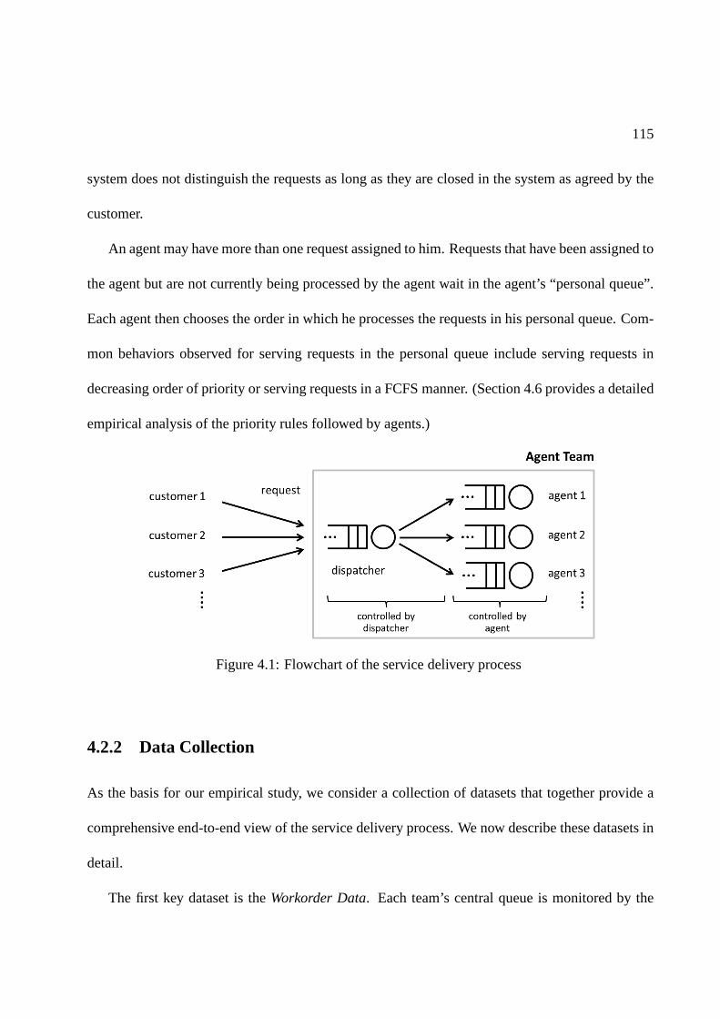
115

system does not distinguish the requests as long as they are closed in the system as agreed by the

customer.

An agent may have more than one request assigned to him. Requests that have been assigned to

the agent but are not currently being processed by the agent wait in the agent’s “personal queue”.

Each agent then chooses the order in which he processes the requests in his personal queue. Com-

mon behaviors observed for serving requests in the personalqueue include serving requests in

decreasing order of priority or serving requests in a FCFS manner. (Section 4.6 provides a detailed

empirical analysis of the priority rules followed by agents.)

Figure 4.1: Flowchart of the service delivery process

4.2.2 Data Collection

As the basis for our empirical study, we consider a collection of datasets that together provide a

comprehensive end-to-end view of the service delivery process. We now describe these datasets in

detail.

The first key dataset is theWorkorder Data. Each team’s central queue is monitored by the

116

team’s dispatcher to identify new requests that have been routed by the provider to the agent team.

For each new request, the dispatcher creates aworkorder record in the Workorder Data. The

workorder record is used to monitor service progress on the request as it is being served by the

agent team. Fields in the workorder record include the request type, complexity, priority, customer,

request creation date and time, and agent to whom the requestis assigned. The workorder record

also records the time that the request is completed. This information is populated by the agent

upon completion of the request. Analysis of the Workorder Data enables a full characterization of

the portfolio of requests waiting in each agent’s personal queue at any point in time.

The second key dataset is theTiming Data, which is gathered for the purpose of understanding

the effort required to serve the different requests handledby the agents in the teams. Data collec-

tion in each team extended for approximately one month. (Theactual time period during which

data was collected varied across the different teams.) During the data collection time period in

each agent team, each agent in the team recorded detailed time intervals he spent on all business-

related activities, including handling different requests, communicating with group members, or

even lunch and breaks. The agent recorded each time he started any business related activity,

paused the activity (for reasons such as to start a differentactivity or to take a break), and when

he completed an activity. Thus the Timing Data provides detailed information on each agent’s

time allocation among different activities and the order inwhich agents prioritize activities. This

unique data-set provides a perfect resource to study agents’ time allocation behavior, the request

processing order, and the variation in their productivity over time.

Table 4.1 lists three sample records from the Timing Data. Each record in the Timing Data

corresponds to a single “session”, or uninterrupted interval of time that the agent allocated to an

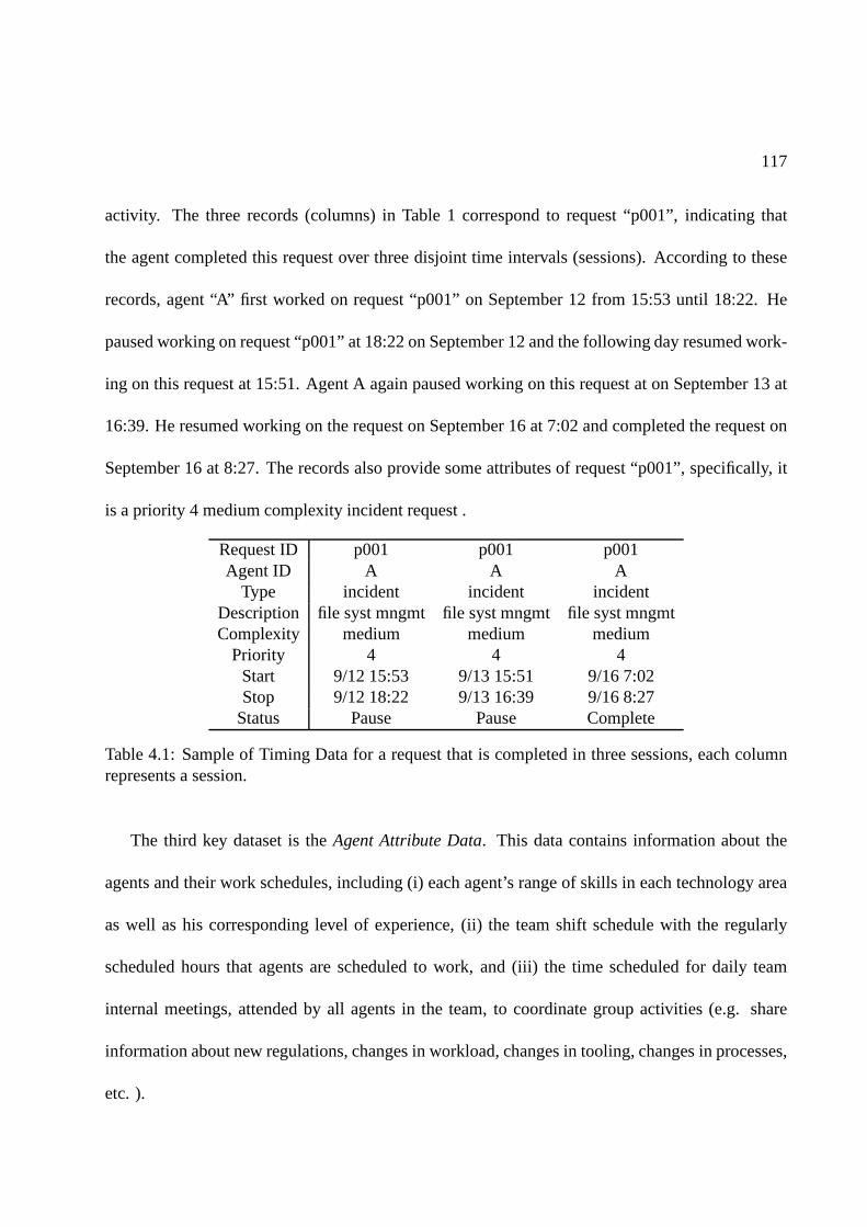
117

activity. The three records (columns) in Table 1 correspondto request “p001”, indicating that

the agent completed this request over three disjoint time intervals (sessions). According to these

records, agent “A” first worked on request “p001” on September 12 from 15:53 until 18:22. He

paused working on request “p001” at 18:22 on September 12 andthe following day resumed work-

ing on this request at 15:51. Agent A again paused working on this request at on September 13 at

16:39. He resumed working on the request on September 16 at 7:02 and completed the request on

September 16 at 8:27. The records also provide some attributes of request “p001”, specifically, it

is a priority 4 medium complexity incident request .

Request ID p001 p001 p001Agent ID A A A

Type incident incident incidentDescription file syst mngmt file syst mngmt file syst mngmtComplexity medium medium medium

Priority 4 4 4Start 9/12 15:53 9/13 15:51 9/16 7:02Stop 9/12 18:22 9/13 16:39 9/16 8:27

Status Pause Pause Complete

Table 4.1: Sample of Timing Data for a request that is completed in three sessions, each columnrepresents a session.

The third key dataset is theAgent Attribute Data. This data contains information about the

agents and their work schedules, including (i) each agent’srange of skills in each technology area

as well as his corresponding level of experience, (ii) the team shift schedule with the regularly

scheduled hours that agents are scheduled to work, and (iii)the time scheduled for daily team

internal meetings, attended by all agents in the team, to coordinate group activities (e.g. share

information about new regulations, changes in workload, changes in tooling, changes in processes,

etc. ).

118

As is common when working with large data-sets, significant effort was required to eliminate

inaccurate records in the data-sets and link these multiplelarge datasets. A key challenge was that

no systematic methods were employed across all of the data sources to record key information

such as a unique request identifier. This challenge in removing inaccuracies from the data-sets and

linking the data-sets is exacerbated when performing empirical analysis in a globally distributed

problem setting. Time stamp fields in the data collected in the different data sources and in the dif-

ferent geographically dispersed agent teams was associated with different time zones, such as the

server system time zone (time zone for the server system storing the data), agent team time zone,

customer time zone, etc. Appendix C.1 details the various statistical methods that we employed to

link the various data sets and eliminate data inconsistencies.

4.2.3 Sample Selection and Summary Statistics

In this section we describe the selection of the sample agentteam for this study and some summary

statistics describing the type of requests processed by theteam.

Our main empirical analysis is focused on a single agent teamwhich is located in India, and

provides 24/7 service for a single customer. We chose this team because its agents keep track of the

unique request identifier very well in the timing study, which enables us to link a high percentage

(92%) of the sessions in the Timing Data with the corresponding workorder records (see appendix

C.1 for details). The focal team has 62 agents of whom 59% havelow experience level, 27% have

medium experience level, and the remaining 14% are comprised of highly experienced agents.

The Timing Data was collected for three weeks during September 2011; during this time 19,089

records (sessions) were recorded. About 70% of the workloadserved by the team are incident

119

requests. Change requests, representing the next largest category of requests in the Workload Data

(30%), are typically jointly scheduled by the customer and provider (rather than controllable by the

agents or dispatcher) and therefore not of interest in our study of how agents organize workload.

Project requests represent less than 1% of the requests processed by the agent team. Although

the agent teams serve multiple types of requests, we focus our empirical study of agents’ working

productivity and their practices for managing workload on incident requests, because the time and

the duration of change requests are typically pre-scheduled and are beyond the agent’s control.

A total of 5049 incidents were recorded during the three weekstudy period. Only about 0.1%

of these incidents are labeled with the highest priority level, priority 1. Priority 2 incidents account

for 25% of the overall incident requests and have a significantly stricter SLA relative to priority

3 and 4 incidents. Our analysis of the Timing Data revealed that it is common for an agent to

interrupt service of a request for reasons such as agent waiting for a customer response, lunch or

break, attending a team meeting, encountering the end of a shift, or switch to serve a different

request. About 33% of the incident requests were interrupted at least once prior to completion,

and it took on average 1.69 sessions to complete an incident request. The average time to process

an incident request, excluding interruptions, was 62 minutes, with a standard deviation of 108

minutes. Consequently, it is common for factors such as agent’s workload level to vary during the

the service time of a request. In fact, we see that for 20% of the incident requests, the variation

of the size of the agent’s personal queue exceeds 3 during theservice time of the request. We

will discuss this time-dependent feature of productivity in greater detail when we introduce our

productivity measure.

Significant effort was spent in matching records between thetiming study data and the work-

120

load data (see C.1). We successfully matched 92% of the sessions in the Timing Data with the

corresponding records in the Workorder Data, but only 71% ofall incident requests recorded in

the Workorder Data for our representative agent team could be linked with corresponding records

in the Timing Data. This is because the agents did not record all their activities in the Timing Data

with complete information. This linking rate is lower (42%)for priority 1 requests, suggesting that

agents fail to record their activities or populate the request identifier more frequently when han-

dling these most urgent requests. The linking rates for priority 2-4 requests are similar and range

between 68%-71%. The linking rates for requests of different complexity levels are also similar

and range between 67%-72%. Therefore, requests recorded inthe timing study actually represent a

sample of all the requests that were processed during the timing study period. Although we did find

the matching rate to be lower for the most urgent (priority 1)requests, they only represent 0.1%

of all incident requests. For the remaining incident requests, the linking rates are consistent across

requests with different priorities and complexity levels,requests that are assigned at different time

of the day, and requests that are handled by different agents. Therefore, we expect these matched

requests to represent all the incident requests assigned tothis agent team, and the findings of the

productivity analysis based on these matched requests to have general implications for the team’s

request management policy.

4.3 Econometric Model of Agent’s Productivity

In this section we describe an econometric model we developed based on the Timing Data to study

the effect of factors influencing an agent’s productivity. We first provide a modeling framework to

121

measure changes in agents’ productivity over time which is suitable for the context of our appli-

cation. Then, based on an exhaustive revision of previous research analyzing worker productivity,

we describe the main factors we hypothesize to affect productivity, and how our proposed produc-

tivity measure can help to disentangle the different mechanisms by which workload may impact

productivity.

4.3.1 Measuring Productivity

Request completion time or its reciprocal, throughput rate, have traditionally been used in the

Operations Management literature as measures of productivity (KC (2012), KC and Terwiesch

(2009), Staats and Gino (2012)). However, the IT service delivery environment analyzed in this

study has several characteristics that require a differentapproach to measure productivity. First,

the total service time of the incidencerequests is relatively long and factors that impact productivity

such as workload levels may fluctuate considerably during this time interval. Such fluctuation of

productivity within the completion time of a request needs to be considered in this study, but it is

challenging to measure using request completion time or throughput rate. Second, the IT service

requests are highly heterogeneous since each request has different features (complexity, priority,

and the matching with the agent’s skill level). These features have different impacts on the request

service time. Consequently, general throughput rates may not accurately capture the impact of

the mixture of different types of requests on an agent’s productivity. The intangible and interactive

nature of the service outputs are also discussed in Djellal and Gallouj (2012) as a challenge to mea-

sure productivity in general service industries, where productivity can not be measured by simply

counting the output in units. Finally, measures such as throughput rates and request completion

122

time capture the overall impact of workload on productivity. Using these measures to identify the

impact of interruptions, which is one of the mechanisms we seek to explore, is challenging. This

is because longer requests are more likely to be interrupted, the positive correlation between total

completion time and the number of interruptions cannot be interpreted as a causal effect. Hence, a

different measure of productivity is needed to study the impact of these interruptions.

To address these challenges, we propose using thehazard rateof the request processing time as

a measure of productivity. Hazard rate, a concept in survival analysis, is defined as the failure rate

at timet conditional on survival until timet. In our setting, failure corresponds to the completion

of a request. More formally, letT denote the total effective processing time of a request (excluding

interruption periods). The hazard rate, expressed as a function of time t, is defined asλ(t) =

limdt→0Pr(t≤T<t+dt)

Pr(t≤T ). The total request processing time can also be recovered in terms of the

hazard rate by the formulaE[T ] =∫∞0exp(−

∫ t

0λ(s)ds)dt. Intuitively, the hazard rate can be

interpreted as the instantaneous rate at which the request is being processed. Modeling productivity

as hazard rates allows productivity to fluctuate during the lifetime of a request and the possibility

to explore the impact of time-varying factors including workload and interruptions. Estimating the

parameters of a hazard rate model requires detailed information on the specific activities an agent

is performing at any given time; this information is accurately provided in our Timing Data.

We estimate the dynamic of the hazard rate using the Cox proportional hazard rate model, as

originally discussed in Breslow (1975), Cox (1972). The hazard rate for agenti who is processing

requestj at timet, denoted asλij(t), is modeled as:

λij(t) = λ0(t′ijt)e

β′Xijt (4.3.1)

123

In equation 4.3.1,t′ijt is the cumulative time that agenti has spent on requestj up to time

t, andλ0(·) is a non-parametric baseline hazard rate function that flexibly captures the common

fluctuation trends of hazard rates when processing all the requests. Explanatory variablesXijt

may be time-dependent and affect the hazard rate in an exponential form, with the coefficientsβ

to be estimated from the data. The model 4.3.1 can be efficiently estimated by maximizing par-

tial likelihoods and the inferences of maximum likelihood estimates can be obtained accordingly

(Kalbfleisch and Prentice (2002)). Next, we discuss the set of factors affecting productivity that

are included in covariatesXt.

4.3.2 Factors Influencing Productivity

We are interested in measuring the impact of factors that canbe controlled through the design of

the SDS on agent productivity. In this subsection, we discuss evidence from previous work to

formulate a set of hypotheses related to the different mechanisms by which workload may affect

productivity and develop metrics to test these hypotheses in the context of our application.

Concurrent workload level

The first mechanism hypothesizes that an agent’s service rate is affected by his workload level.

Laboratory experiments (Schultz et al. (1999, 1998)) show that workers in Just-In-Time production

systems exhibit shorter processing times as their own inputbuffer (or workload level) increases,

which indicates that workers will work faster if they are thebottleneck of the flow line. KC (2012)

analyzes the data collected in a hospital emergency room andfinds that physician’s throughput rate

increases as he is seeing more patients.

In the context of our application, it is plausible for agentsto adjust their service rate at which

124

they process requests. The agent may incur a higher “cognitive” cost when working at a higher

service rate, and adjust the service rate dynamically to attain the required SLAs while minimizing

their time-average cognitive cost. Intuitively, it is moreefficient to speed-up when the queue is

longer, because the additional cognitive effort has a higher impact on the total waiting time of the

requests in queue. (George and Harrison (2001) shows conditions under which the optimal service

rate increases with the queue length.)

While the aforementioned studies suggest productivity increases at higher workload levels,

other studies suggest that productivity may drop. Workloadlevels may generate stress that hurts

workers’ productivity, as shown in Dahl (2010). Holstrom (1994), Schmenner (1988) study indus-

trial statistics and find that productivity, measured by theoutput per employee, is inversely related

to lead time, suggesting that higher workload levels reduceproductivity.

The combination of these different impacts can lead to non-linear and non-monotone effects

of concurrent workload on worker productivity, as Kuntz et al. (2012) shows in an empirical study

using hospital data. To capture the effect of these different potential impacts related to the agent’s

concurrent workload, we defineWKLDit as the number of unfinished requests assigned to agent

i at timet ,that is, the request in the agent’s personal queue. We include both a linear and quadratic

term ofWKLD in the model to capture non-monotonicities.

An agent’s productivity may also be impacted by his co-workers’ workload level in addition

to his own. For example, the laboratory experiments conducted by Schultz et al. (1999, 1998),

which replicate an industrial production line, find that workers adjust their productivity depending

on the inventory of other workers in the production line. In another experimental study, Schultz

et al. (2003) finds that when performance feedback is available such that workers can see the

125

performance of others, their productivity increases. KC and Terwiesch (2009) shows that higher

system workload levels lead to shorter patient transportation times within the hospitals and shorter

length of stay of cardiac surgery patients in a medical hospital. The field experiment conducted

by Bandiera et al. (2012) discovers that workers, especially the slower ones, work faster when

feedback is available.

In the context of our study, agents do not directly observe the queues of the other agents in

their team. but they may still share this information through personal communications. We define,

TEAMWKLDt =∑

j WKLDjt, which aggregates all the requests in the team members’ per-

sonal queues. We include the linear and quadratic term ofTEAMWKLD in the model to capture

the impact of the entire team’s concurrent workload level onagent’s productivity.

Accumulated workload

In a longer time-span, sustained workload by an agent generates work accumulation which can

induce further effects on his productivity. One mechanism relates to accumulated experience is

that it can lead to productivity gains through a learning-by-doing effect. This learning-by-doing

effect has long been recognized (Wright (1936)). Several recent studies also provide empirical

support for this effect. For example, Pisano et al. (2001) finds that cumulative experience leads

to higher productivity, and the rate of this learning effectvaries across hospitals based on a study

of cardiac surgery data. More recently, Gans et al. (2012) studies call center data and identifies

different patterns in agents’ learning curves.

On the other hand, long periods of sustained high workload can induce reductions in produc-

tivity due to fatigue. For example, KC and Terwiesch (2009) finds that although high workload can

induce short-term boosts to productivity, sustained above-average workload levels lead to drops in

126

productivity. Caldwell (2001), Setyawati (1995) also find similar phenomenon for aircrews and

production workers, where fatigue causes diminishing productivity.

Our study spans a relatively short-time horizon – three weeks – which provides limited time

for agents to experience long-term learning. We observe, however, significant differences in the

experience among the agents. These differences are controlled throughagent fixed effects, which

are included in our model specification. In addition, we alsocontrol for short-term learning ef-

fects during the span of a worker shift, through the covariateCUMWORK which measures the

number of hours since the start of the current shift. The square ofCUMWORK is also included

to capture a potential non-linear/non-monotone effects ofthis variable– for example, after long

working hours, productivity may decay due to a fatigue effect.

Request specialization

In addition to thevolumeof workload, we explore the impact of the diversity/varietyof work-

load on agent productivity. Staats and Gino (2012) providesa comprehensive review of different

mechanisms by which request specialization may influence productivity. An important benefit of

request specialization is that the number of changeovers isreduced, thereby decreasing the num-

ber of adjustments in the cognitive process associated withswitching between dissimilar requests.

(This is analogous to the switching time incurred for a machine to change its production modes

(Bailey (1989)).)

The Timing Data provides detailed information on an agent’srequest switching activities. Each

record in the Timing Data contains a description of the associated request, which can be used to

define a measure of similarity between requests and track when an agent switches between different

types of requests. Two requests are considered similar if they have the same request description and

127

the same type (e.g., both are incidence requests with the description “file system management”).

The dummy variableSAMEWORK indicates whether the request under execution was preceded

by a session when the agent is processing a similar request, ignoring breaks or other non-request-

related activities in between. If changeover costs betweendifferent requests are substantial, we

would expect to see a positive effect ofSAMEWORK on productivity.

Focus, a concept introduced by Skinner (1974), is another mechanism through which request

specialization can benefit productivity. Developing expertise in a narrower set of requests can

facilitate process improvement efforts and thereby achieve higher efficiency. The degree of focus

can be typically defined at different hierarchical levels within an organization: for example, in

the healthcare application studied by KC and Terwiesch (2011), specialization can be defined at

a hospital level (e.g., a cardiac-specialty hospital), at the service department level (e.g., a cardiac

service specialized in revascularization procedures), orat the doctor level (e.g., a cardiac surgeon

that focuses on a specific type of procedure or technique).

In the context of the SDS in our study, the degree of specialization can be defined at both the

agent team and the agent level. Team specialization is kept fixed in our study because the empirical

analysis focuses on a representative team. However, different agents in this representative team

focus on different skill levels: some agents have expertisein more technical skills, and likewise,

requests are classified according to the required skill level needed to solve the problem. Hence,

a request is considered to be within the focused expertise set of an agent if the specified request

skill level matches his skill level. We measure “focus mismatch” with two dummy variables,

SKILLBELOW andSKILLABOV E, indicating whether whether the skill of the agent is

128

below or above the request’s required skill level (when the request and agent skills match, both

indicators are equal to zero).

Interruptions

The Timing Data also enables us to identify various types of interruptions which occur during

an agents’ working hours. The impact of interruptions is important to explore because productivity

may be indirectly impacted by agents’ workload levels through the impact of interruptions as fol-

lows: First, higher workload may increase the likelihood oflonger and more frequent interruptions

of certain types. Second, the occurrence and the length of certain interruptions may have varying

impact on productivity. For example, some interruptions may break the agent’s working rhythm

and incur a set-up cost upon resuming (DeMarco and Lister (1999), Schultz et al. (2003), Spira and

Feintuch (2005)), others may work as a physical relaxation and increase the productivity (Henning

et al. (1997)).

In our study, we seek to measure both the magnitude and the duration of the impact of different

types of interruptions on productivity. Some interruptions cause an agent to pause all his work-

ing activities and may potentially impact all the succeeding activities. We identify two classes

of such interruptions, including: (i) lunch or breaks and (ii) regular team meetings (described in

section 4.2.2). We index these two classes of interruptionsasBreak, Team, and measure their

impacts on the productivity forall the sessions that occur after these interruptions. Anotherset of

interruptions refer to the scenario when an uncompleted request is suspended and resumed after

a period of time. During this period of time, an agent can perform any activities such as taking

breaks or working on other requests. Based on the length of the suspending period, we clas-

sify these interruptions into two classes, and measure their impacts on the productivity when the

129

request is resumed after such an interruption. These interruptions include (iii) over-night interrup-

tions, where the suspending period contains at least one endof the working shift; (iv) same-shift

interruptions, where the suspending period lies in the sameworking shift. We index them as

multishift,sameshift respectively. Since the effect of interruptions is likely to be temporary, we

measure its effect through a set of lagged dummy variables, defined asITRPTijt(c, l), which in-

dicate whether agenti works on requestj at timet after an interruption of classc which occurred

l periods ago, wherec ∈break,team,multishift,sameshift. Lagged time periods are defined by

6 ten-minute intervals within an hour. The length of breaks and team meeting interruptions typ-

ically do not vary much, however, for the second set of interruptions when unfinished requests

are suspended, their impact on productivity is also likely to be related to the length of the sus-

pending time due to forgetting. Therefore, forc ∈multishift,sameshift, we measure the impact

usingITRPTijt(c, l) · Lengthijt(c), whereLengthijt(c) is the length of the suspending period

after which agenti resumes requestj measured in hours.

Control variables

In addition, our specification includes several control variables. Request complexity is captured

through a set of dummy variables indicating three levels of complexity (the lowest level excluded

as the base level). Similarly, we include a set of dummy variables capturing three levels of request

priority (lowest priority excluded as the base level). To capture seasonal effects, we include a set

of dummy variables indicating weekdays/weekends and hour-of-the-day (12 blocks of two-hour

periods) and all their interactions.

The summary statistics of the aforementioned factors are reported in table 4.2.

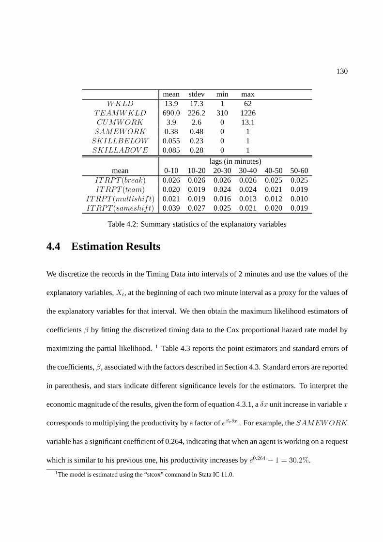
130

mean stdev min maxWKLD 13.9 17.3 1 62

TEAMWKLD 690.0 226.2 310 1226CUMWORK 3.9 2.6 0 13.1SAMEWORK 0.38 0.48 0 1SKILLBELOW 0.055 0.23 0 1SKILLABOV E 0.085 0.28 0 1

lags (in minutes)mean 0-10 10-20 20-30 30-40 40-50 50-60

ITRPT (break) 0.026 0.026 0.026 0.026 0.025 0.025ITRPT (team) 0.020 0.019 0.024 0.024 0.021 0.019

ITRPT (multishift) 0.021 0.019 0.016 0.013 0.012 0.010ITRPT (sameshift) 0.039 0.027 0.025 0.021 0.020 0.019

Table 4.2: Summary statistics of the explanatory variables

4.4 Estimation Results

We discretize the records in the Timing Data into intervals of 2 minutes and use the values of the

explanatory variables,Xt, at the beginning of each two minute interval as a proxy for the values of

the explanatory variables for that interval. We then obtainthe maximum likelihood estimators of

coefficientsβ by fitting the discretized timing data to the Cox proportional hazard rate model by

maximizing the partial likelihood.1 Table 4.3 reports the point estimators and standard errors of

the coefficients,β, associated with the factors described in Section 4.3. Standard errors are reported

in parenthesis, and stars indicate different significance levels for the estimators. To interpret the

economic magnitude of the results, given the form of equation 4.3.1, aδx unit increase in variablex

corresponds to multiplying the productivity by a factor ofeβxδx . For example, theSAMEWORK

variable has a significant coefficient of 0.264, indicating that when an agent is working on a request

which is similar to his previous one, his productivity increases bye0.264 − 1 = 30.2%.

1The model is estimated using the “stcox” command in Stata IC 11.0.

131

variableX βX (X − X)2

WKLD 0.0178*** -8.01e-4***(3.70e-3) (1.96e-4)

TEAMWKLD -1.63e-4 -6.05e-7(1.32e-4) (4.61e-7)

CUMWORK 0.0387*** -3.02e-3(0.0131) (-3.71e-3)

SAMEWORK 0.264***(0.0519)

SKILLBELOW -0.610(0.554)

SKILLABOV E 1.38*(0.794)

lags (in minutes)0-10 10-20 20-30 30-40 40-50 50-60

ITRPT 0.326*** 0.292*** 0.118 0.137 0.201 0.139(break) (0.123) (0.105) (0.111) (0.112) (0.126) (0.104)ITRPT 0.225 -0.204 0.175 0.520*** 0.472*** 0.212(team) (0.155) (0.210) (0.151) (0.136) (0.144) (0.159)

ITRPT · Length -0.0236*** -8.46e-3*** -6.83e-3* -6.13e-4 3.25e-3 2.79e-3(multishift) (5.57e-3) (3.06e-3) (3.61e-3) (2.69e-3) (2.25e-3) (3.21e-3)

ITRPT · Length -0.179*** -0.0755 -0.0821 0.0376 0.0937 -0.0309(sameshift) (0.0649) (0.0663) (0.0735) (0.0591) (0.0759) (0.0607)

Table 4.3: Estimation results of the cox proportional hazard rate model. Standard errors in paren-thesis. Stars indicate the significance level, *** for 0.01,** for 0.05, and * for 0.1.

Concurrent workload level

The results in Table 4.3 indicate that workload, as measuredby the size of an agent’s personal

queue, impacts productivity. In Figure 4.2, we provide a plot of agent productivity (as measured

by hazard rate of request handling time) as a function of the size of an agent’s personal queue.

For the ease of comparison, the productivity when the personal queue contains only 1 request is

normalized to be 1. The solid line provides the measure of productivity; the dashed lines represent

the 95% confidence interval. Productivity increases with the size of an agent’s personal queue, and

132

peaks as the size of an agent’s personal queue approaches 25;with this level of workload an agent’s

productivity can be 60% higher than when his personal queue is empty. The marginal increase in

productivity becomes smaller and diminishes as the size of an agent’s personal queue exceeds 25

requests. Interestingly, the team’s workload level does not have significant impact on individual

agent’s productivity. These results provide evidence thatagents increases their speed of processing

requests when their concurrent workload level increases, but the increase of speed diminishes as

workload level exceeds some threshold. The overall relationship between individual workload and

productivity suggests that it is beneficial for the dispatcher to ensure that agents have some requests

in their personal queues.

5 10 15 20 25 30 35 401

1.1

1.2

1.3

1.4

1.5

1.6

1.7

1.8

1.9

2productivity vs. workload level

concurrent workload level

haza

rd r

ate

Figure 4.2: Plot of impact of size of agent’s personal queue on agent’s productivity (dashed linesrepresent the 95% confidence interval)

To further explore its managerial insights, it is useful to check if there is heterogeneity in

133

this relationship among different agents. If different groups of agents respond to the workload in

different ways, the dispatcher would respond by applying different request allocation policies to

each group. We therefore estimate the relationship betweenindividual workload and productivity

for sub-groups of agents with different skill levels, and find the results to be robust and consistent

for these sub-groups. Namely, productivity increases concavely with individual workload, while

the team’s workload has no significant impact on agent’s productivity. The policy insights of these

findings will be further discussed in section 4.5.

Accumulated workload

The variableCUMWORK reflects the time duration since the start of the agent’s current shift,

and the impact of this explanatory variable evaluates agentproductivity at different times since the

start of the agent’s shift. Here, use of the hazard rate modelis particularly critical to capture the

dynamic nature of this variable. Our analysis indicates that the coefficient ofCUMWORK is

significant. Figure 4.3 displays a plot of agent productivity as a function of the number of hours

that have elapsed since the start of the agent’s shift based on the results in Table 4.3. The solid line

represents the measure of productivity; the dashed lines represent the 95% confidence bounds. The

shape of the curve indicates that productivity increases (agents work faster) at the end of the shift.

(We note that the typical length of a shift is nine hours). This is consistent with a learning effect

associated with higher cumulative workload (Halm et al. (2002), Pisano et al. (2001)).

Request specialization

Our analysis also shows that similarity of consecutive requests processed by an agent impacts

agent productivity. As indicated in Table 4.3, the coefficient of SAMEWORK is statistically

significant with a coefficient of0.264. The interpretation of this coefficient is that an agent’s

134

0 1 2 3 4 5 6 7 8 91

1.1

1.2

1.3

1.4

1.5

1.6

1.7

1.8

1.9

2productivity vs. cumulative workload

time since the start of the shift (hrs)

haza

rd r

ate

Figure 4.3: Productivity variation at different times of a shift (dash lines represent the 95% confi-dence interval)

productivity is on average 30% higher when processing a request that is similar to the previous

request he processed. This suggests that specialization isbeneficial in the short term, and the

dispatcher may consider assigning similar requests to the same agent. The finding that short-term

specialization improves productivity is consistent with the findings of Staats and Gino (2012).

Interruptions

Finally, the estimates of lagged dummies for the different classes of interruptions have different

signs, indicating that the different classes of interruptions have different impacts on the productiv-

ity. Further, the impacts on productivity are temporary since all the estimates become statistically

insignificant for dummies with longer lags. More specifically, interruptions of classbreak, have a

positive temporary impact on productivity. A higher productivity is observed for the first twenty

135

minutes after an agent returns from a lunch or break session.This increased level of productivity

may be explained by the relaxation of physical discomfort and mental stress during long periods

of computer work (Henning et al. (1997)). Interruptions caused by team meetings also increase

productivity; the effect is observed 30-50 minutes after the start of the team huddle meeting. Since

team meetings are scheduled to last for about thirty minutes, the result of our analysis is consistent

with an increase in productivity for the first twenty minutesfollowing a team meeting. This finding

is consistent with the objective of team huddle meetings, which encourages agents to communicate

and help each other with their work.

In contrast, the estimates forITRPT (multishift)·Length andITRPT (sameshift)·Length

indicate that request suspending periods exhibit a negative impact on productivity, and such neg-

ative impact is more pronounced for longer interruptions. For example, during the first 10 min-

utes when an agent resumes a request following a 24-hour overnight interruption, he works1 −

e−0.0236∗24 = 43% slower. It takes another 10 minutes before the agent recovers his normal speed of

work. This reduced level of productivity may be explained bythe set-up or recovery time required

for an agent to revisit a request and remind himself of the particulars of the request (DeMarco and

Lister (1999), Spira and Feintuch (2005)). It is worth pointing out that many of these findings, such

as the temporary impact of interruptions on agent productivity, are natural products of the hazard

rate analysis and the Timing Data, and would otherwise be difficult to obtain if one only studies

the service completion time or throughput rate.

To understand how interruptions are related to the impact ofworkload on productivity and

its implication for the request allocation policy, we also need to explore how workload levels

impact the frequency and length of different types of interruptions. Team huddle meetings and

136

lunch breaks are either pre-scheduled or unavoidable in nature, and hence can be considered to

be exogenous. In appendix C.2, we study the relationship between workload and the second set

of interruptions where requests are suspended. Interestingly, our analysis reveals that higher in-

dividual workload levels are associated with longer suspending periods. The frequency of these

interruptions, on the other hand, are not impacted by the workload level. This indicates another

type of cost associated with high workload levels: assigning many requests to an agent prolongs

the revisit time for suspended requests, which reduces the agent’s productivity when he revisit the

request.

4.5 Impact of Workload on Request Allocation Policies

The findings in section 4.4 indicates higher levels of workload are associated with increased agent

productivity. In this section we discuss how these findings can be integrated into request allocation

policies in SDS’s to positively impact agent productivity through a simulation study.

State-dependent service rates like this have been discussed in analytical literature. Crabill

(1972) and George and Harrison (2001) examined the optimal control policy for anM/M/1 queue

with state-dependent service rates, where the tradeoff is customers’ waiting cost and the cost asso-

ciated with different service rates. Cachon and Zhang (2006, 2007a) analyzed the tradeoff between

incentives to provide faster service and the correspondingcost in a queueing model with two strate-

gic servers. Girbert and Weng (1998)investigated a two-server queuing system where the servers

are self-interested and can adjust their service rate. Girbert and Weng (1998) compared two cus-

tomer allocation strategies: common queue and separate queues and showed that separate queues

137

can create strong incentives for individual servers to speed up. van Olijen and Bertrand (2003)

investigated a system where service rate increases and thendecreases with workload, and showed

that the performance of the system could be improved by implementing an arrival-rate control pol-

icy. Bekker and Borst (2006) considered anM/G/1 queue where the service rate is first increasing

and then decreasing as a function of the workload and found the optimal admission control policy.

We now explore the implications of this finding for optimal request allocation in an SDS. Specif-

ically, we consider three alternative request allocation mechanisms: (i) thedecentralized system,

where the dispatcher does not hold any requests and assigns each request to an agent upon arrival,

(ii) the centralized system, where the dispatcher maintains a central queue of requestsand assigns

requests to agents as agents become available, and (iii) thestream system, where agents are sep-

arated into teams that serve a dedicated request class(es).Note that in an SDS, we distinguish

between actions that are controlled by the dispatcher and those controlled by the agents in the

agent team. While the dispatcher determines the time at which requests are assigned to agents as

well as to which agent each request should be assigned, each agent independently determines the

order in which to serve requests in his personal queue. We nowdescribe these alternative systems

in greater detail.

Under thedecentralized system, the dispatcher immediately assigns each arriving requestto

the agent with the smallest personal queue. The benefit of this allocation policy is that it takes full

advantage of the productivity boost achieved by higher workload levels, by maintaining all requests

in the personal agent queues. However, a decentralized system has potential shortcomings. First, it

reduces the SDS to a parallel queueing system, which is less efficient in utilizing service capacities

compared to a multi-server pooled system. This operationalinefficiency is small, however, because

138

of the join-shortest-queue criteria. Second, a request with long service time will delay all the

remaining requests in the agent’s personal queue, reducingfairness of the system.

Under thecentralized system, the dispatcher holds all the incoming requests in a centralqueue,

and prioritizes high-priority requests. When an agent becomes available the dispatcher assigns him

the first request from the prioritized central queue. The centralized system provides the operational

benefit of resource pooling. On the other hand, it is unable tobenefit from the productivity boost

gained by long personal queues since requests are retained in the dispatcher’s central queue. De-

pending on the magnitude of the impact of workload on productivity, the productivity loss of the

centralized system could be quite considerable.

Under thestream system,agents are divided into groups and each group is dedicated toserve

one subset of request classes. Within each group, the dispatcher assigns arriving requests to the

agent with the shortest personal queue. Stream systems are often implemented when there is a

desire to provide “special” or “fast track” service to a subset of request classes. The concept

of stream systems has been introduced in Emergency Departments (Saghafian et al. (2012),Welch

(2008)) to more efficiently provide medical care to urgent patients. Although stream systems result

in some loss of resource pooling, it allows for dedicated service to high priority request classes with

short target times. Depending on the relative volumes of arriving workload for the different request

classes, a stream system may introduce imbalanced workloadfor the different groups of agents.

In the remainder of this section, we describe the results of asimulation study where we explore

the performance of these three systems to gain greater insight into the implications of the impact

of workload on request allocation policies. We consider an agent team that, for ease of exposition,

serves two classes of requests:h and l, whereh requests have higher priority overl requests.

139

Requests arrive according to independent Poisson processes with rateλh =5/hr andλl=15/hr and

join a central queue managed by a dispatcher. The requests are subject to contractual SLAs which

specify thatpi ∈ (0, 1) of typei requests must be completed withinai time units, (i ∈ h, l). The

SLA requirements for typeh requests are stricter than those for typel requests:ph > pl, ah < al.

The goal of the service system is to meet SLA requirements forboth request classes. Specifically,

the SLAs require that 95% of theh requests must be completed within 4 hours from the time that

the request arrives to the system and 80% of thel requests must be completed within 48 hours

of when the request arrives to the system. The composition and the SLAs of requests of the two

priority levels are set according to the observed value in our study period.

The dispatcher decideswhenrequests are assigned to agents as well as towhomeach request

should be assigned. Each agent independently controls the order in which he processes the requests

that have been assigned to him. In this section, we consider the ideal situation where agents adopt

the following two rules: (i)h requests are prioritized overl requests and (ii) requests of the same

class are processed according to FCFS order. Furthermore, we assume each agent’s service rate

changes with his workload following the relationship demonstrated in Figure 4.2, and their service

rates are normalized to 1 request/hr with empty workload levels.

We simulate performance of this SDS under the three request allocation policies. For each

policy, we simulate 100,000 arriving requests and measure service level performance for the two

types of requests. Table 4.4 reports on the minimum number ofagents required to meet the SLAs

under each of the three request allocation policies. The decentralized system requires a minimum

of 13 agents. With this level of staffing 95% ofh requests are completed in 3.3 hours and 80% of

l requests are completed in 19.4 hours, achieving the contractual SLAs. The centralized system

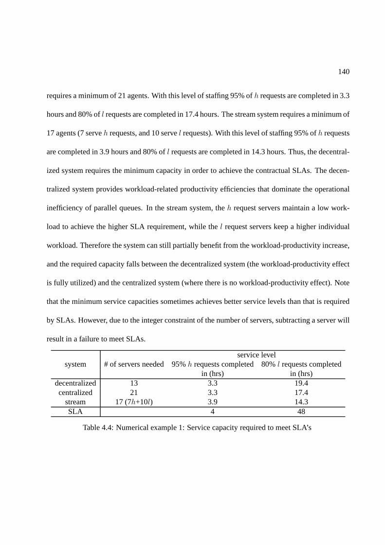
140

requires a minimum of 21 agents. With this level of staffing 95% ofh requests are completed in 3.3

hours and 80% ofl requests are completed in 17.4 hours. The stream system requires a minimum of

17 agents (7 serveh requests, and 10 servel requests). With this level of staffing 95% ofh requests

are completed in 3.9 hours and 80% ofl requests are completed in 14.3 hours. Thus, the decentral-

ized system requires the minimum capacity in order to achieve the contractual SLAs. The decen-

tralized system provides workload-related productivity efficiencies that dominate the operational

inefficiency of parallel queues. In the stream system, theh request servers maintain a low work-

load to achieve the higher SLA requirement, while thel request servers keep a higher individual

workload. Therefore the system can still partially benefit from the workload-productivity increase,

and the required capacity falls between the decentralized system (the workload-productivity effect

is fully utilized) and the centralized system (where there is no workload-productivity effect). Note

that the minimum service capacities sometimes achieves better service levels than that is required

by SLAs. However, due to the integer constraint of the numberof servers, subtracting a server will

result in a failure to meet SLAs.

service levelsystem # of servers needed 95%h requests completed 80%l requests completed

in (hrs) in (hrs)decentralized 13 3.3 19.4centralized 21 3.3 17.4

stream 17 (7h+10l) 3.9 14.3SLA 4 48

Table 4.4: Numerical example 1: Service capacity required to meet SLA’s

141

4.6 Accounting for Agent’s Priority Schemes

In this section, we explore insights for the request allocation policy considering both the workload

effect and the agent’s behavior of managing his processing order. The results presented in Table

4.4 are based on the assumption that agents strictly prioritizeh requests overl requests and process

requests following the FCFS rule, which is an ideal and efficient order to process requests. More

realistically, once the dispatcher assigns requests to an agent’s personal queue, it is challenging for

the dispatcher or provider to control how an agent manages the workload in his personal queue and

each agent will adopt his preferred policy. The order in which each agent processes the requests

affects the waiting time of requests and thus the service level performance. In this section, we

will explore how agents manage to process the requests in practice, and extend the results of our

analysis presented in Table 4.4 by considering alternativerules by which agents may manage the

requests in their personal queues.

4.6.1 Agent Choice Model

We begin by describing a model to empirically study how an agent manages requests in his per-

sonal queue. At any point in time, the agent’s workload management problem can be decomposed

into two decisions: (i) how long to serve the request he is currently serving, and (ii) which request

to serve next. The first decision (time to serve the request currently in service) is not fully con-

trolled by the agent. Service is typically not interrupted unless exogenous factors such as the need

to wait for a customer input, encountering unexpected problems or unavoidable interruptions, cus-

tomer demanding immediate response, scheduled meetings, etc. The second decision is typically

142

controlled by the agent and more relevant to the processing order. We develop the following choice

model to study the agent’s behavior of managing the order in which he processes requests.

Conditional on an agent starting to process a new request in his personal queue, we use a

conditional logit model to describe his choice of the request to process. More specifically, assume

agenti decides to start processing a new request at timet, and let choice setJit contain all the

unprocessed requests in his personal queue at timet. For each jobj ∈ Jit, the utility for agenti to

choose it is

Uitj = Xitjβ + ǫitj (4.6.1)

In equation 4.6.1,ǫijt is a double-exponentially distributed error term following standard as-

sumptions. We include the following explanatory variablesXijt.

The first variable represents the arriving order of the request, denoted asORDERitj, and is

calculated by (requestj’s order of arriving inJit)/(number of requests inJit). It lies in (0, 1]

and reflects the relative order of requestj in Jit. The request withORDERitj = 1 is the one

assigned to agenti most recently. If agents prioritize first-come requests, a negative coefficient

will be expected. The second variable represents the severity level of the request. We useSEV kj

as the binary indicator of requestj being a priorityk request,k = 1, 2, · · · , 4. Given that priority

1 requests only account for 0.1% in population, we combined them with priority 2 requests as

a group of high priority requests. Finally, we include theSAMEWORKijt variable to account

for the fact that agents may manage to process similar requests together. The binary variable

143

SAMEWORKijt = 1 if the candidate requestj is similar to the request previously served by

agenti before timet, and 0 otherwise.

Following the standard assumptions of logistic regressions, the probability for agenti to choose

requestj ∈ Jit to process next follows the logistic function formPitj =eXitjβ

∑k∈Jit

eXitkβ .We estimate

the logit model 4.6.1 using empirical data, and MLE results of the coefficients are reported in Ta-

ble 4.5. The standard error of the estimators are reported inthe parenthesis, and the star codes

follow the same rule as in Table 4.3. The choice model predicts 18% of the choice successfully

in the sample, with a pseudoR2 of 3.2%. VariableORDER has a significant odds ratio of 0.784,

which indicates that the last-come request is on average 22%less likely to be picked by the agent

comparing to the first-come request in the queue. The indicator of high priority requestsSEV 1,2

has a significant positive coefficient 1.472, showing that a high priority request is about 47% more

likely to be chosen than a low priority request, given that they arrive at the same time. Priority

3 requests are not significantly prioritized over priority 4requests, which is not surprising since

both of these requests are less priority requests. Similarly, theSAMEWORK coefficient is also

insignificant, indicating that agents do not prioritize to group similar requests together. In sum-

mary, the estimation results indicate that agents give slight priority to requests that arrive earlier

and requests with higher priority, but significant uncertainty remains in their choices. We test the

same model on sub-groups of agents grouping by their skill level, and find consistent results.

4.6.2 Impact of Processing Order on Request Allocation Policies

Similar to section 4.5, we again consider three request allocation policies, but now accounting for

the agent’s prioritizing behavior. That is, agents no longer follow strict prioritizing rules nor FCFS

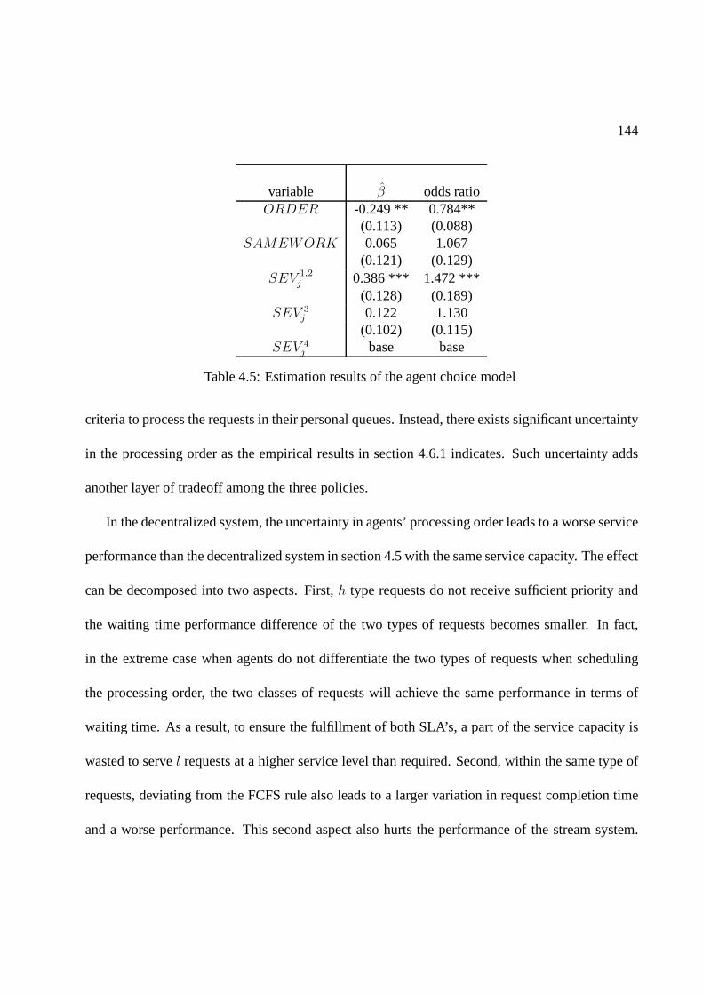
144

variable β odds ratioORDER -0.249 ** 0.784**

(0.113) (0.088)SAMEWORK 0.065 1.067

(0.121) (0.129)SEV 1,2

j 0.386 *** 1.472 ***(0.128) (0.189)

SEV 3j 0.122 1.130

(0.102) (0.115)SEV 4

j base base

Table 4.5: Estimation results of the agent choice model

criteria to process the requests in their personal queues. Instead, there exists significant uncertainty

in the processing order as the empirical results in section 4.6.1 indicates. Such uncertainty adds

another layer of tradeoff among the three policies.

In the decentralized system, the uncertainty in agents’ processing order leads to a worse service

performance than the decentralized system in section 4.5 with the same service capacity. The effect

can be decomposed into two aspects. First,h type requests do not receive sufficient priority and

the waiting time performance difference of the two types of requests becomes smaller. In fact,

in the extreme case when agents do not differentiate the two types of requests when scheduling

the processing order, the two classes of requests will achieve the same performance in terms of

waiting time. As a result, to ensure the fulfillment of both SLA’s, a part of the service capacity is

wasted to servel requests at a higher service level than required. Second, within the same type of

requests, deviating from the FCFS rule also leads to a largervariation in request completion time

and a worse performance. This second aspect also hurts the performance of the stream system.

145

In the centralized system, the performance remains the samebecause the dispatcher holds all the

incoming requests and decides the processing order centrally.

In the remainder of this section, we conduct a simulation study to explore the insights of the

performance of the three systems when both the impact of workload effect and the uncertainty

in agents’ processing order are present. The settings are the same as the first simulation study in

section 4.5, except that now the agent chooses the next request to process according to the the

estimation result obtained in Table 4.5 rather than the FCFSrule.

In table 4.6, we compare the minimal number of servers required under each allocation pol-

icy to meet the SLA’s. As table 4.6 indicates, the results forthe centralized system remains the

same. The number of servers needed in the stream system is still the same, but the service levels,

measured by thepi quantile of request completion time, are longer. This is dueto the deviation

from the FCFS order. The decentralized system’s performance is affected the most. It now needs

23 (previously 13) servers to meet both SLA’s. Notice that because of the inefficient processing

order, a substantial amount of service capacity is actuallywasted since typel requests are now

completed at a much quicker time than required by its SLA. In this example, the stream system

requires the least number of servers because it takes advantage of both the workload-productivity

effect (within agent groups), and the flexibility to controlthe performance of different types of

requests by adjusting the size of agent groups.

146

service levelsystem # of servers needed 95%h requests completed 80%l requests completed

in (hrs) in (hrs)decentralized 24 3.8 2.1centralized 21 3.3 17.4

stream 18 (8h+10l) 3.6 17.9SLA 4 48

Table 4.6: Numerical example 2: Service capacity required to meet SLA’s

4.7 Conclusion

In this study, we seek to explore the impact of workload levels on productivity from a distinct point

of view. To do this, we utilize the Timing Data, a new dataset which tracks the time intervals agents

spend on specific activities, to study agent’s productivityin a SDS. Based on the econometric

techniques from survival analysis, we are able to develop a new methodology to measure agent’s

productivity, which incorporates the time dependent feature of the productivity. This approach

enables us to identify different mechanisms by which workload levels impact productivity, which

provides important implications for the workload allocation policy.

We examine the impact of workload on productivity through four factors: the concurrent work-

load level, the accumulative workload level, specialization of the workload composition, and dif-

ferent types of interruptions. Our first finding indicates a nonlinear relationship between an agent’s

concurrent workload level and his speed of work: agents temporarily increase their processing

speed when facing a longer personal queue, but the marginal increase diminishes as the queues

grow longer. This provides the dispatcher with the incentive to assign requests to agents earlier in

order to keep agents’ personal queues longer. In terms of theaccumulated workload, we identify

an increase in productivity as workload accumulates in the working shift. Higher productivity can

147

also be achieved when the agent specializes his work on similar requests, suggesting the benefit of

short-term specialization and focus. This provides incentive for the dispatcher to assign similar re-

quests to each agent, an implication regarding managing thecomposition of the agent’s workload

in addition to its volume. Finally, we also find different types of interruptions to have different

temporary impacts on agent productivity. Such effort of quantifying both the magnitude and the

effective time of the impact of interruptions based on data of a real SDS, to our best knowledge,

has not been done before.

In light of these findings, we further integrate the feature of workload-dependent service rates

into the SDS’s request allocation policy. We explore the trade-off between three commonly ob-

served request allocation systems (the decentralized, centralized, and steam system) through a

simulation study. We illustrate the insights by analyzing ateam that serves requests of two priory

levels and compare the minimal number of servers required tomeet the different SLAs associ-

ated with the two priority levels. There are essentially twofactors determining the performance

of the service time: the service speed, which is impacted by the individual workload level, and

the processing order, which is determined by the agent or thedispatcher depending on the alloca-

tion policy. Consequently, the dispatcher’s decision on when to assign requests needs to account

for two competing goals: earlier allocation leads to higherindividual workload levels and faster

service rates; while late allocation ensures the dispatcher to have better control of the request pro-

cessing order. The control of the processing order is particularly important when there is much

randomness when agents are managing their own processing order, as is the case in this study. Our

example demonstrates how the request allocation time and the randomness in agent’s processing

order can have significant impact on the team’s service levelperformance.

148

We believe the findings and the methodology presented in thisstudy can motivate further re-

search on productivity in the context of service operationsand beyond. For example, there may

exist unobservable factors affecting an agent’s workload management behavior, and well-designed

field experiments are useful to investigate these factors and validate the outcome of different re-

quest allocation policies. Applying analytical tools to understand them is another potential research

direction. In summary, productivity analysis has always been an important issue in operations

management, and we believe that the present study provides deeper understanding of some of the

behavioral phenomena of worker productivity as well as powerful insights for future research.

Bibliography

Afanasyev, M., H. Mendelson. 2010. Service provider competition: Delay cost structure, segmentation, andcost advantage.Manufacturing & Service Operations Management12(2) 213–235.

Afeche, P., H. Mendelson. 2004. Pricing and priority auctions in queueing systems with a generalized delaycost structure.Management Science869–882.

Agency, Central Intelligence. 2012. The world factbook: Gdp composition by sector. URLhttps://www.cia.gov/library/publications/the-world-factbook/fields/2012.html.

AHRQ Brief. 2006. Bioterrorism and Health System Preparedness: Issue Briefs. Agency for HealthcareResearch and Quality, Rockville, MD. URLwww.ahrq.gov/news/ulp/btbriefs/.

Aksin-Karaesmen, Zeynep, Baris Ata, Seyed Emadi, Che-Lin Su. 2011. Structural Estimation of CallersDelay Sensitivity in Call Centers. Working paper.

Allon, Gad, Awi Federgruen, Margaret Pierson. 2011. How Much Is a Reduction of Your Customers’ WaitWorth? An Empirical Study of the Fast-Food Drive-Thru Industry Based on Structural EstimationMethods.Manufacturing and Service Operations Management13(4) 489–507.

American Association of Neurological Surgeons. 2005. Cerebrovascular disease. URLwww.aans.org/PatientInformation/ConditionsandTreatments/CerebrovascularDisease.aspx.

American Burn Association. 2009. National Burn RepositoryReport of Data from 1999-2008.

Antonides, Gerrit, Peter C. Verhoef, Marcel van Aalst. 2002. Consumer Perception and Evaluation ofWaiting Time: A Field Experiment.Journal of Consumer Psychology12(3) 193–202.

Argon, N.T., S. Ziya. 2009. Priority assignment under imperfect information on customer type identities.MSOM11 674–693.

Argon, N.T., S. Ziya, R. Righter. 2008. Scheduling impatient jobs in a clearing system with insights onpatient triage in mass-casualty incidents.Probability in the Engineering and Informational Sciences22 301–332.

Bailey, Charles D. 1989. Forgetting and the learning curve:A laboratory study.Management science35(3)340–352.

Bandiera, O., I. Barankay, I. Rasul. 2012. Team Incentives:Evidence from a Firm Level Experiment.working paper.

Bekker, R., S.C. Borst. 2006. Optimal admission control in queues with workload-dependent service rates.Probability in the Engineering and Informational Sciences20(4) 543–570.

Bell, D.R., J.M. Lattin. 1998. Shopping behavior and consumer preference for store price format: Why”large basket” shoppers prefer EDLP.Marketing Science17(1) 66–88.

149

https://www.cia.gov/library/publications/the-world-factbook/fields/2012.html



www.ahrq.gov/news/ulp/btbriefs/

www.aans.org/Patient Information/Conditions and Treatments/Cerebrovascular Disease.aspx



150

Berry, L.L., K. Seiders, D. Grewal. 2002. Understanding service convenience.Journal of Marketing66(3)1–17.

BF, Stewart, Siscovick D, Lind BK, Gardin JM, Gottdiener JS,Smith VE. 1997. Clinical factors associatedwith calcific aortic valve disease. Cardiovascular Health Study. J Am Coll Cardiol29 630–634.

Bloomberg, Michael R., Thomas R. Frieden. 2007. HIV epidemiology and field services semiannual report.NYC Department of Health and Mental Hygiene.

Boxma, O.J., F.G. Forst. 1986. Minimizing the epected weighted number of tardy jobs in stochastic flowshops.Operations Research Letters5 119–126.

Bravata, D.M., G.S. Zaric, J.C. Holty, M.L. Brandeau, E.R. Wilhelm, K.M. McDonald, D.K. Owens. 2006.Reducing mortality from anthrax bioterrorism: Strategiesfor stockpiling and dispensing medical andpharmaceutical supplies.Biosecurity and Bioterrorism: Biodefense Strategy, Practice, and Science4244–262.

Breslow, N.E. 1975. Analysis of Survival Data under the Proportional Hazards Model.InternationalStatistical Review43(1) 45–57.

Brown, L., N. Gans, A. Mandelbaum, A. Sakov, H. Shen, S. Zeltyn, L. Zhao. 2005. Statistical analysis of atelephone call center: A queueing-science perspective.Journal of the American Statistical Association100(469) 36–50.

Bucklin, R.E, J.M. Lattin. 1991. A two-state model of purchase incidence and brand choice.MarketingScience1024–39.

Buyukkoc, C, P. Varaiya, J. Walrand. 1985. Thec − µ rule revisited.Advances in Applied Probability17237–238.

Cachon, G.P., F. Zhang. 2006. Procuring Fast Delivery: SoleSourcing with Information Asymmetry.Management Science52(6) 881–896.

Cachon, G.P., F. Zhang. 2007a. Obtaining Fast Service in a Queueing System via Performance-BasedAllocation of Demand.Management Science53(3) 408–420.

Cachon, G.P., F. Zhang. 2007b. Obtaining fast service in a queueing system via performance-based alloca-tion of demand.Management Science53(3) 408.

Caldwell, T.B. 2001. The impact of fatigue in air medical andother types of operations: a review of fatiguefacts and potential countermeasures.Air Medical Journal1(20) 25–32.

Campbell, D., F. Frei. 2010. Market Heterogeneity and LocalCapacity Decisions in Services.Manufactur-ing & Service Operations Management.

Carmon, Ziv. 1991. Recent studies of time in consumer behavior. Advances in Consumer Research18(1)703–705.

Chandon, P., V.G. Morwitz, W.J. Reinartz. 2005. Do intentions really predict behavior? Self-generatedvalidity effects in survey research.Journal of Marketing69(2) 1–14.

Chim, H., W. S. Yew, C. Song. 2007. Managing burn victims of suicide bombing attacks: outcomes, lessonslearnt, and changes made from three attacks in Indonesia.Critical Care11 R15.

Committee on Trauma. 1999. Resources for optimal care of theburn injured patient.American College ofSurgeons.

Cox, D.R. 1972. Regression Models and Life-Tables.Journal of the Royal Statistical Society34(2) 187–220.

Crabill, T.B. 1972. Optimal control of a service facility with variable exponential service times and constantarrival rate.Management Science18(9) 560–566.

151

Curreri, P. W., A. Luterman, D. W. Braun, G. T. Shires. 1980. Burn injury. Analysis of survival and hospi-talization time for 937 patients.Annals of Surgery192472–478.

Dahl, Michael S. 2010. Organizational Change and Employee Stress.Management Science57(2) 240–256.

Davis, M.M., T.E. Vollmann. 1993. A framework for relating waiting time and customer satisfaction in aservice operation.Journal of Services Marketing4(1) 61–69.

Deacon, Robert T., Jon Sonstelie. 1985. Rationing by Waiting and the Value of Time: Results from a NaturalExperiment.Journal of Political Economy93(4) 627–647.

Debo, Laurens, Senthil Veeraraghavan. 2009.Consumer-Driven Demand and Operations Management, vol.131, chap. 4 , Models of Herding Behavior in Operations Management. Springer Science, 81–111.

DeMarco, T., T. Lister. 1999.Peopleware: Productive Projects and Teams (Second Edition). Dorset House.

Djellal, F., F. Gallouj. 2012. Beyond Productivity Measurement and Strategies: Performance Evaluation andStrategies in Services .Working paper.

Emedicine health. 2010. Peripheral vascular disease. URLwww.emedicinehealth.com/peripheral_vascular_disease/article_em.htm.

Epilepsy Foundation. 2010. Epilepsy and seizure statistics. URLwww.epilepsyfoundation.org/about/statistics.cfm.

Fader, P.S., B.G.S Hardie. 1996. Modeling Consumer Choice Among SKUs.Journal of Marketing Reserach33(4) 442–452.

Faulin, J., A.A. Juan, S.E. Grasman, M.J. Fry. 2012.Decision Making in Service Industries: A PracticalApproach. CRC Press.

Fisher, M.L., J. Krishnan, S. Netessine. 2009. Are your staffing levels correct? International CommerceReview8(2) 110–115.

Flegal, M., M. D. Carroll, C. L. Ogden, L. R. Curtin. 2010. Prevalence and trends in obesity among USadults, 1999-2008.The Journal of the American Medical Association235–241.

Forbes, S.J. 2008. The effect of air traffic delays on airlineprices. International Journal of IndustrialOrganization26(5) 1218–1232.

Forst, F.G. 2010. Minimizing the expected weighted number of tardy jobs with non-identically distributedprocessing times and due dates.Research in Business and Economics Journal2 1–7.

Frank, Christopher. 2012. Improving decision making in theworld of big data.URL http://www.forbes.com/sites/christopherfrank/2012/03/25/improving-decision-making-in-the-world-of-big-data/.

Fund for Public Health in New York, Inc. 2005. NYC Bioterrorism Hospital Preparedness Program: HospitalPreparedness Task Force For Patients with Burns. Request for Proposals.

Gans, N., G. Koole, A. Mandelbaum. 2003. Telephone call centers: Tutorial, review, and research prospects.Manufacturing and Service Operations Management5(2) 79–141.

Gans, N., N. Liu, A. Mandelbaum, H. Shen, H. Ye. 2012. ServiceTimes in Call Centers: Agent Hetero-geneity and Learning with some Operational Consequences.working paper.

George, J.M., J.M. Harrison. 2001. Dynamic control of a queue with adjustable service rate.OperationsResearch49(5) 720–731.

Girbert, S.M., A.K. Weng. 1998. .Incentive Effects Favor Nonconsolidating Queues in a Service System:The Principal Agent Perspective44(12) 1662–1669.

www.emedicinehealth.com/peripheral_vascular_disease/article_em.htm

www.emedicinehealth.com/peripheral_vascular_disease/article_em.htm

www.epilepsyfoundation.org/about/statistics.cfm

www.epilepsyfoundation.org/about/statistics.cfm

http://www.forbes.com/sites/christopherfrank/2012/03/25/improving-decision-making-in-the-world-of-big-data/

http://www.forbes.com/sites/christopherfrank/2012/03/25/improving-decision-making-in-the-world-of-big-data/

152

Glazebrook, K. D., P. S. Ansell, R. T. Dunn, R. R. Lumley. 2004. On the optimal allocation of service toimpatient tasks.Journal of Applied Probability4151–72.

Gross, D., J. Shortle, J. Thompson, C. Harris. 2008.Queueing Theory. 4th ed. Wiley.

Guadagni, P.M., J.D.C. Little. 1983. A logit model of brand choice calibrated on scanner data.MarketingScience2 203–238.

Halm, E.A., C. Lee, M.R. Chassin. 2002. Is volume related to outcome in health care? A systematic reviewand methodologic critique of the literature.Annals of Internal Medicine137(6) 511–521.

Hasija, S., E. Pinker, R. Shumsky. 2008. Call center outsourcing contracts under information assymetry.Management Science54(4)793–807.

Henning, R.A., P. Jacques, G.V. Kissel, A.B. Sullivan, S.M.Alteras-Webb. 1997. Frequent short rest breaksfrom computer work: effects on productivity and well-beingat two field sites. Ergonomics40(1)78–91.

Heskett, James L., Thomas O. Jones, Gary W. Loveman, W. Earl Sasser, Leonard A. Schlesinger. 1994.Putting the service-profit chain to work.Harvard Business Review72(2) 164–174.

Hess, S., M. Bierlaire, J.W. Polak. 2005. Estimation of value of travel-time savings using mixed logitmodels.Transportation Research Part A: Policy and Practice39(2-3) 221–236.

Holstrom, J. 1994. The relationship between speed and productivity in industry networks: A study ofindustrial statistics.Int. J. Production Economics34 91–97.

Hui, Michael K., David K. Tse. 1996. What to Tell Consumers inWaits of Different Lengths: An IntegrativeModel of Service Evaluation.The Journal of Marketing60(2) 81–90.

Hui, M.K., Dube Laurette, Jean-Charles Chebat. 1997. The impact of music on consumers reactions towaiting for services.Journal of Retailing73(1) 87–104.

Hui, S.K., P.S. Fader, E.T. Bradlow. 2009. The traveling salesman goes shopping: The systematic deviationsof grocery paths from tsp optimality.Marketing Science28(3) 566–572.

Ibrahim, Rouba, Ward Whitt. 2011. Wait-Time Predictors forCustomer Service Systems with Time-VaryingDemand and Capacity.Operations Research59(5) 1106–1118.

Janakiraman, Narayan, Robert J. Meyer, Stephen J. Hoch. 2011. The Psychology of Decisions to AbandonWaits for Service.Journal of Marketing Research48 970–984.

Jang, W., C. M. Klein. 2002. Minimizing the expected number of tardy jobs when processing times arenormally distributed.Operations Research Letters30 100–106.

Jansen, L. A., S. L. Hynes, S. A. Macadam, A. Papp. 2012. Reduced Length of Stay in Hospital for BurnPatients Following a Change in Practice Guidelines: Financial Implications.J Burn Care Researchtoappear.

Jassal, D., S. Sharma, B. Maycher. 2009. Pulmonary hypertension imaging.Emedicine.

Kalbfleisch, J.D., R.L. Prentice. 2002.The statistical analysis of failure time data, Second edition. Wiley.

Katz, Karen, M. Larson Blaire, Larson R C. 1994. Prescription for the waiting-in-line blues: Enlighten,entertain, and engage.Sloan Management Review32(2) 44–53.

KC, D.S. 2012. Does Multi-Tasking Improve Productivity andQuality? Evidence from the EmergencyDepartment .working paper.

Kc, D.S., C. Terwiesch. 2009. Impact of workload on service time and patient safety: An econometricanalysis of hospital operations.Management Science55(9) 1486–1498.

153

KC, D.S., C. Terwiesch. 2009. Impact of Workload on Service Time and Patient Safety: An EconometricAnalysis of Hospital Operations.Management Science55(9) 1486–1498.

KC, D.S., C. Terwiesch. 2011. The Effects of Focus on Performance: Evidence from California Hospitals .Management Science57(11) 1898–1912.

Kenessey, Zoltan. 1987. The primary, secondary, tertiary and quaternary sectors of the economy.Review ofIncome and Wealth33(4) 359–385.

Kulkarni, V.G. 1995.Modeling and analysis of stochastic systems. Chapman & Hall/CRC.

Kuntz, L., R. Mennicken, S. Scholtes. 2012. Stress on the ward: An empirical study of the nonlinearrelationship between organizational workload and servicequality. working paper.

Larson, J.S., E.T. Bradlow, P.S. Fader. 2005. An exploratory look at supermarket shopping paths.Interna-tional Journal of research in Marketing22(4) 395–414.

Larson, R.C. 1987. Perspective on queues: Social justice and the psychology of queueing.OperationsResearch35(6) 895–905.

Leahy, N. E., R. W. Yurt, E. J. Lazar, A. A. Villacara, A. C. Rabbitts, L. Berger, C. Chan, L. Chertoff, K. M.Conlon, A. Cooper, L. V. Green, B. Greenstein, Y. Lu, S. Miller, F. P. Mineo, D. Pruitt, D. S. Ribaudo,C. Ruhren, S. H. Silber, L. Soloff. 2011. Burn Disaster Response Planning in New York City: UpdatedRecommendations for Best Practices.J Burn Care Researchto appear.

Lee, E.K., C.-H. Chen, F. Pietz, B. Benecke. 2009. Modeling and optimizing the public-health infrastructurefor emergency response.Interfaces39 476–490.

Lozano, Daniel. 2012. Medical Director, Lehigh Valley Healthcare Network regional burn center. PrivateCommunication.

Mahoney, E.J., D.R. Harrington, W.L. Biffl, J. Metzger, T. Oka, W. G. Cioffi. 2005. Lessons learned from anightclub fire: Institutional disaster preparedness.Journal of Trauma-Injury Infection & Critical Care58 487–491.

Mandelbaum, A., S. Zeltyn. 2004. The impact of customers patience on delay and abandonment: Someempirically-driven experiments with the mmng queue.OR Spectrum26(3) 377–411.

National Inst. on Alcohol Abuse and Alcoholism. 2004. 2001-2002 National Epidemiologic Survey onAlcohol and Related Conditions. URLwww.niaaa.nih.gov/NewsEvents/NewsReleases/Pages/NESARCNews.aspx#chart.

Neslin, S.A., H.J. van Heerde. 2008. Promotion dynamics.Foundations and Trends in Marketing3 (4)177–268.

NYC Department of Health and Mental Hygiene. 2008. EpiQuery: NYC interactive health data. URLa816-healthpsi.nyc.gov/epiquery/EpiQuery/index.html.

NYC Dept. of Health and Mental Hygiene. 2007. Hepatitis A, B and C Surveillance Report, NewYork City, 2006 and 2007. URLwww.nyc.gov/html/doh/downloads/pdf/dires/dires-2008-report-semi1.pdf.

NYS Department of Health. 2000. The burden of cardiovascular disease in new york: Mortality, preva-lence, risk factors, costs and selected populations. URLwww.health.ny.gov/diseases/cardiovascular/heart_disease/docs/burden_of_cvd_in_nys.pdf.

NYS Department of Health. 2004. Dementias Reported in Hospitalizations Among New YorkState Residents. URLwww.health.state.ny.us/diseases/conditions/dementia/alzheimer/dementia_registry.htm.

www.niaaa.nih.gov/NewsEvents/NewsReleases/Pages/NESARCNews.aspx#chart

www.niaaa.nih.gov/NewsEvents/NewsReleases/Pages/NESARCNews.aspx#chart

a816-healthpsi.nyc.gov/epiquery/EpiQuery/index.html

www.nyc.gov/html/doh/downloads/pdf/dires/dires-2008-report-semi1.pdf

www.nyc.gov/html/doh/downloads/pdf/dires/dires-2008-report-semi1.pdf

www.health.ny.gov/diseases/cardiovascular/heart_disease/docs/burden_of_cvd_in_nys.pdf

www.health.ny.gov/diseases/cardiovascular/heart_disease/docs/burden_of_cvd_in_nys.pdf

www.health.state.ny.us/diseases/conditions/dementia/alzheimer/dementia_registry.htm

www.health.state.ny.us/diseases/conditions/dementia/alzheimer/dementia_registry.htm

154

NYS Department of Health. 2007. New York State Cancer Registry Estimated Cancer Prevalence by Site ofCancer and Gender, 2007. URLwww.health.ny.gov/statistics/cancer/registry/pdf/table8.pdf.

NYS Department of Health. 2008. New York Diabetes Prevalence Data (BRFSS). URLwww.nyshealthfoundation.org/content/document/detail/1148/.

Osler, T., L. G. Glance, D. W. Hosmer. 2010. Simplified Estimates of the Probability of Death After BurnInjuries: Extending and Updating the Baux Score.J Trauma68 690–697.

Osler, T., L. G. Glance, D. W. Hosmer. 2011. Comparison of Hospital Mortality Rates After Burn Injury inNew York State: A Risk-Adjusted Population-Based Observational Study.J Trauma71 1040–1047.

Perdikaki, O., S. Kesavan, J.M. Swaminathan. 2012. Effect of traffic on sales and conversion rates of retailstores.Manufacturing & Service Operations Management14(1) 145–162.

Pinedo, M. 2008.Scheduling Theory, Algorithms, and Systems. Springer.

Pisano, P., R.M.J. Bohmer, A.C. Edmondson. 2001. Organizational diferences in rates of learning: evidencefrom the adoption of minimally invasive cardiac surgery.Management Science47(6) 752–768.

Png, I.P.L., D. Reitman. 1994. Service time competition.The Rand Journal of Economics25(4) 619–634.

Rao, B.M., M.J.M. Posner. 1987. Algorithmic and approximation analyses of the shorter queue model.Naval Research Logistics34381–398.

Rossi, P.E., G.M. Allenby. 2003. Bayesian statictics and marketing. Marketing Science22 (3)304–328.

Rossi, P.E., R.E. McCulloch, G.M. Allenby. 1996. The value of purchase history data in target marketing.Marketing Science15 321–240.

Rothkopf, M.H., P. Rech. 1987. Perspectives on queues: Combining queues is not always beneficial.Oper-ations Research35(6) 906–909.

Saffle, J. R., N. Gibran, M. Jordan. 2005. Defining the ratio ofoutcomes to resources for triage of burnpatients in mass casualties.J Burn Care Rehabil26 478–482.

Saghafian, S., W. Hopp, M. Van Oyen, J. Desmond, S. Kronick. 2011. Complexity-Based Triage: A Toolfor Improving Patient Safety and Operational Efficiency.Working Paper, University of Michigan.

Saghafian, S., W.J. Hopp, M.P. Van Oyen, J.S. Desmond, S.L. Kronick. 2012. Patient Streaming as aMechanism for Improving Responsiveness in Emergency Departments . Operations Research60(5)1080–1097.

Saydah, S, M Eberhardt, N Rios-Burrows, D Williams, L Geiss.2007. Prevalence of Chronic KidneyDisease and Associated Risk Factors - United States 1999-2004. J Burn Care Res56 161–165.

Schmenner, R.W. 1988. The merit of making things fast.Sloan Management Review8 11–17.

Schultz, K.L., D.C. Juran, J.W. Boudreau. 1999. The effectsof low inventory on the development of pro-ductivity norms.Management Science45(12) 1664–1678.

Schultz, K.L., D.C. Juran, J.W. Boudreau, J.O. McClain, L.J. Thomas. 1998. Modeling and worker motiva-tion in JIT production systems.Management Science44(12) 1595–1607.

Schultz, K.L., J.O. McClain, L.J. Thomas. 2003. Overcomingthe darkside of workerflexibility .Journal ofOperations Management21(1) 81–92.

Setyawati, L. 1995. Relation between feelings of fatigue, reaction time and work productivity.J. Hum.Ergol (Tokyo)1(24) 129–135.

www.health.ny.gov/statistics/cancer/registry/pdf/table8.pdf

www.health.ny.gov/statistics/cancer/registry/pdf/table8.pdf

www.nyshealthfoundation.org/content/document/detail/1148/

www.nyshealthfoundation.org/content/document/detail/1148/

155

Sheridan, R., J Wber, K Prelack, L. Petras, M. Lydon, R. Tompkins. 1999. Early burn center transfershortens the length of hospitilization and reduces complications in children with serious burn injuries.J Burn Care Rehabil20347–50.

Skinner, Wickham. 1974.The focused factory. Harvard Business Review.

Spira, J.B., J.B. Feintuch. 2005. Spira, Jonathan B., and Joshua B. Feintuch. ”The cost of not paying atten-tion: How interruptions impact knowledge worker productivity.” Report from Basex (2005).Reportfrom Basex.

Staats, B.R., F. Gino. 2012. Specialization and Variety in Repetitive Tasks: Evidence from a Japanese Bank.Management Science58(6) 1141–1159.

Steinberg, R.A., C. Rudd, S. Lacy, A. Hanna. 2011.IT Infrastructure library service operations. TheStationery Office.

Tapson, Victor F., Marc Humbert. 2006. Incidence and prevalence of chronic thromboembolic pulmonaryhypertension.The Proceedings of the American Thoracic Society564–567.

Taylor, Shirley. 1994. Waiting for Service: The Relationship between Delays and Evaluations of Service.The Journal of Marketing58(2) 56–69.

Thombs, B. D., V. A. Singh, J. Halonen, A. Diallo, S. M. Milner. 2007. The effects of preexisting medicalcomorbidities on mortality and length of hospital stay in acute burn injury: Evidence from a nationalsample of 31,338 adult patients.Annals of Surgery245(4) 629–634.

Train, K. 2003.Discrete choice methods with simulation. Cambridge Univ Press.

U.S. Department of Health and Human Services. 2008. National survey on drug use and health. URLwww.oas.samhsa.gov/nhsda.htm.

van Mieghem, J.A. 1995. Dynamic scheduling with convex delay costs: The generalizedc|µ rule. TheAnnals of Applied Probability5 809–833.

van Olijen, H.P.G., J.W.M. Bertrand. 2003. The effects of a simple arrival rate control policy on throughputand work-in-process in production systems with workload dependent processing rates.Int. J. Produc-tion Economics85 61–68.

Wang, S. C. 2010. Michigan?s plan for burn mass-casualty incidents. URL http://www.advocatehealth.com/documents/trauma/Regional%20Burn%20Response_Wang.pdf.

Wein, L. M., Y. Choi, S. Denuit. 2010. Analyzing evacuation versus shelter-in-place strategies after aterrorist nuclear detonation.Risk Analysis30 1315–1327.

Welch, S.J. 2008. Patient segmentation: Redisigning flow.Emergency Medicine News31(8).

Wright, T.P. 1936. Factors affecting the costs of airplanes. Journal of Aeronautical Science1(3) 122–128.

Wrongdiagnosis. 2011a. Prevalence and incidence of arrhythmias. URLwww.wrongdiagnosis.com/a/arrhythmias/prevalence.htm.

Wrongdiagnosis. 2011b. Prevalence and incidence of paralysis. URLwww.wrongdiagnosis.com/p/paralysis/prevalence.htm.

Wrongdiagnosis. 2011c. Prevalence and incidence of pepticulcer. URLwww.wrongdiagnosis.com/p/peptic_ulcer/prevalence.htm.

Yurt, R. W., P. Q. Bessey, G. J. Bauer, R. Dembicki, H. Laznick, N. Alden, A. Rabbits. 2005. A RegionalBurn Center?s Response to a Disaster: September 11, 2001, and the Days Beyond.J Burn CareRehabil26 117–124.

www.oas.samhsa.gov/nhsda.htm

www.oas.samhsa.gov/nhsda.htm

http://www.advocatehealth.com/documents/trauma/Regional%20Burn%20Response_Wang.pdf



www.wrongdiagnosis.com/a/arrhythmias/prevalence.htm

www.wrongdiagnosis.com/a/arrhythmias/prevalence.htm

www.wrongdiagnosis.com/p/paralysis/prevalence.htm

www.wrongdiagnosis.com/p/paralysis/prevalence.htm

www.wrongdiagnosis.com/p/peptic_ulcer/prevalence.htm

www.wrongdiagnosis.com/p/peptic_ulcer/prevalence.htm

156

Yurt, R. W., E. J. Lazar, N. E. Leahy, N. V. Cagliuso, A. C. Rabbits, V. Akkapeddi, A. Cooper, A. Dajer,J. Delaney, F. Mineo, S. Silber, L. Soloff, K. Magbitang, D. W. Mozingo. 2008. Burn disaster responseplanning: An urban region’s approach.J Burn Care Rehabil29158–165.

157

Appendix A

Appendix for Chapter 2

A.1 Determining the Distribution for Deli Visit Time

Our estimation method requires integrating over differentpossible values of deli visit time. This

appendix describes how to obtain an approximation of this distribution. Our approach follows

two steps. First, we seek to estimate the distribution of theduration of a supermarket visit. Sec-

ond, based on the store layout and previous research on customer paths in supermarket stores, we

determine (approximately) in which portion of the store visit customers would cross the deli.

In terms of the first step, to get an assessment of the durationof a customer visit to the store,

we conducted some additional empirical analysis using store foot traffic data. Specifically, we

collected data on the number of customers that entered the store during 15 minute intervals (for the

month of February of 2009). With these data, our approach requires discretizing the duration of

a visit in 15 minutes time intervals. Accordingly, letT denote a random variable representing the

duration of visit, from entry until finishing the purchase transaction at the cashier, with support in

158

0, 1, 2, 3, 4, 5, 6. T = 0 is a visit of 15 minutes or less,T = 1 corresponds to a visit between 15

and 30 minutes, and similarly for the other values. Letθt = Pr(T = t) denote the probability mass

function of this random variable. Not all customers that enter the store go through the cashier: with

probabilityψ a customer leaves the store without purchasing anything. Hence,∑6

t=0 θt + ψ = 1.

Note thatθtt=0...6 andψ completely characterize the distribution of the visit duration T .

LetXt be the number of entries observed during periodt andYt the total number of observed

transactions in the cashiers during that period. We have:

E(Yt|Xrr≤t) =6

∑

s=0

Xt−sθs.

Because the conditional expectation ofYt is linear in the contemporaneous and lagged entries

Xt, . . . , Xt−6, the distribution of the duration of the visit can be estimated through the linear re-

gression:

Yt =

6∑

s=0

Xt−sθs + ut.

Note that the regression does not have an intercept. The following table shows the Ordinary Least

Squares estimates of this regression.1

The parametersθ0 throughθ4 are positive and statistically significant (the other parameters are

close to zero and insignificant, so we consider those being equal to zero). Conditional on going

through the cashier, about 70% of the customers spend 45 minutes or less in the store (calculated

as∑2

t=0 θt/∑4

t=0 θt), and 85% of them less than an hour. The average duration of a visit is about

1The parameters of the regression could be constrained to be positive and to sum to less than one. However, in theunconstrained OLS estimates all the parameters that are statistically significant satisfy these constraints.

159

Estimate Std.Err.θ0 0.0689** (0.0209)θ1 0.107** (0.0261)θ2 0.101** (0.0272)θ3 0.0631** (0.0274)θ4 0.0657** (0.0274)θ5 0.0289 (0.0265)θ6 -0.0197 (0.0226)N 879R2 0.928

Table A.1: Regression results for the deli visit time distribution. (* p < 0.1 , ** p < 0.05 )

35 minutes. Moreover, the distribution of the duration of the store visit could be approximated

reasonably well by a uniform distribution with range [0,75]minutes.

To further understand the time at which a customer visits thedeli, it is useful to understand the

path that a customer follows during a store visit. In this regard, the study by Larson et al. (2005)

provides some information of typical customer shopping paths in supermarket stores. They show

that most customers tend to follow a shopping path through the “race-track”– the outer ring of the

store that is common in most supermarket layouts. In fact, the supermarket where we base our

study has the deli section located in the middle of the race-track. Moreover, Hui et al. (2009) show

that customers tend to buy products in a sequence that minimizes total travel distance. Hence, if

customer baskets are evenly distributed through the racetrack, it is likely that the visit to the deli

is done during the middle of the store visit. Given that the visit duration tends to follow a uniform

distribution between [0,75] minutes, we approximate the distribution of deli visit time by a uniform

distribution with range [0,30] minutes before check-out time.

160

Appendix B


B.1 Simulation Model

We now describe the simulation model which is used to analyzevarious scenarios. This simulation

model is based on the mathematical model described in Section 3.4 as well as discussions with burn

physicians. There are currently 140 burn beds in NYC and the surrounding area. These centers

can be flexed up to 210 in a catastrophic event. We simulate a potential event in NYC and consider

how patients are treated and transferred into these 210 Tier1 burn beds. The simulation considers

a time period of 5 days, and makes the following assumptions:

1. The number of beds is fixed at 210.

2. All N patients are available to be transferred at the beginning ofthe horizon. These patients

consist of inpatients only.

3. Patienti has expected LOS,Li. The realization of his LOS is independent of all other patients

161

and is log-normally distributed with location and scale parameters calibrated using the mean

and standard deviation from the National Burn Repository data as summarized in Table 3.4.

4. Patienti is classified as class1 (Ci = 1) if he is a Type 1, 2B, or 3 patient. Otherwise, he is a

Type 2A patient (a Tier 2/3 patient with TBSA less than 20% andno inhalation injury) and

is classified as class2 (Ci = 2)

5. Patienti has benefit,∆Pi = wiPi, which is given by the TIMM model for survival probabil-

ity, Pi, and the deterioration factor given in Table 3.3.

(a) If a class1 patient is transferred into a burn bed within the first3 days, he generates

reward∆Pi. Otherwise, he generates0 benefit.

(b) If a class2 patient is transferred into a burn bed within the first5 days, he generates

reward∆Pi. Otherwise, he generates0 benefit.

Patients are prioritized according to the specified triage algorithm. Patients who are not given a

bed at the beginning of the horizon are assumed to be cared forand stabilized in a Tier 2/3 hospital.

Once a patient departs from the burn center, a new bed becomesavailable. The patient with the

highest triage index is selected from the remaining patients to be transferred into the Tier 1 burn

bed. For each simulation, we generated 10,000 patient cohorts and realizations for LOS.

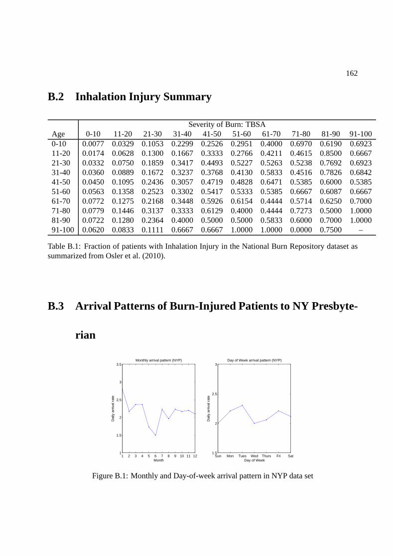
162

B.2 Inhalation Injury Summary

Severity of Burn: TBSAAge 0-10 11-20 21-30 31-40 41-50 51-60 61-70 71-80 81-90 91-1000-10 0.0077 0.0329 0.1053 0.2299 0.2526 0.2951 0.4000 0.6970 0.6190 0.692311-20 0.0174 0.0628 0.1300 0.1667 0.3333 0.2766 0.4211 0.4615 0.8500 0.666721-30 0.0332 0.0750 0.1859 0.3417 0.4493 0.5227 0.5263 0.5238 0.7692 0.692331-40 0.0360 0.0889 0.1672 0.3237 0.3768 0.4130 0.5833 0.4516 0.7826 0.684241-50 0.0450 0.1095 0.2436 0.3057 0.4719 0.4828 0.6471 0.5385 0.6000 0.538551-60 0.0563 0.1358 0.2523 0.3302 0.5417 0.5333 0.5385 0.6667 0.6087 0.666761-70 0.0772 0.1275 0.2168 0.3448 0.5926 0.6154 0.4444 0.5714 0.6250 0.700071-80 0.0779 0.1446 0.3137 0.3333 0.6129 0.4000 0.4444 0.7273 0.5000 1.000081-90 0.0722 0.1280 0.2364 0.4000 0.5000 0.5000 0.5833 0.6000 0.7000 1.000091-100 0.0620 0.0833 0.1111 0.6667 0.6667 1.0000 1.0000 0.0000 0.7500 –

Table B.1: Fraction of patients with Inhalation Injury in the National Burn Repository dataset assummarized from Osler et al. (2010).

B.3 Arrival Patterns of Burn-Injured Patients to NY Presbyt e-

rian

1 2 3 4 5 6 7 8 9 10 11 121

1.5

2

2.5

3

3.5Monthly arrival pattern (NYP)

Dai

ly a

rriv

al r

ate

MonthSun Mon Tues Wed Thurs Fri Sat

1.5

2

2.5

3Day of Week arrival pattern (NYP)

Dai

ly a

rriv

al r

ate

Day of Week

Figure B.1: Monthly and Day-of-week arrival pattern in NYP data set

163

B.4 Resources for Prevalence Data

Prevalence data was obtained from the resources listed in table B.2.

Comorbiditiy ResourceHIV/AIDS Bloomberg and Frieden (2007)Renal disease Saydah et al. (2007)Liver disease NYC Dept. of Health and Mental Hygiene (2007)Metastatic cancer NYS Department of Health (2007)Pulmonary circulation disordersJassal et al. (2009), Tapson and Humbert (2006)Congestive heart failure NYS Department of Health (2000)Obesity Flegal et al. (2010)Malignancy w/o metastasis NYS Department of Health (2007)Peripheral vascular disorders Emedicine health (2010)Alcohol abuse National Inst. on Alcohol Abuse and Alcoholism (2004)Other neurological disorders Epilepsy Foundation (2010)Cardiac arrhythmias Wrongdiagnosis (2011a)Cerebrovascular disease American Association of Neurological Surgeons (2005)Dementia NYS Department of Health (2004)Diabetes NYS Department of Health (2008)Drug abuse U.S. Department of Health and Human Services (2008)Hypertension NYC Department of Health and Mental Hygiene (2008)Paralysis Wrongdiagnosis (2011b)Peptic ulcer disease Wrongdiagnosis (2011c)Valvular disease BF et al. (1997)

Table B.2: Resources for prevalence data.

164

Appendix C


C.1 Data Linking and Cleaning

Significant effort was required to cleaning and link the multiple large data-sets, since no systematic

methods were employed to record key information across all data sources. For example, the unique

identifier used to identify requests was not common across the Timing Data and the Workorder

Data. We employed text matching algorithms to match the textin a free text field in the Timing

Data, which agents often populated with the request unique identifier that is used in the Workorder

Data, to link request records in the Timing Data and Workorder Data. The text matching algorithms

that we employed enabled us to match 92% of the incident-related records in the Timing Data

with their corresponding records in the Workorder Data. We also note that not all the request-

related activities are recorded in the timing data, becauseagents may forget to record some of their

activities in the timing data, especially when they are working on urgent tasks. As a result, 71% of

165

all the incident requests in the Workorder Data were linked with the corresponding activities in the

Timing Data.

As another example, the Team Schedule Data informs on the team schedule but not on the

assignment of agents to specific shifts. It is important to identify the specific shift schedules for

each agent because it is useful to construct explanatory variables such as the agent’s cumulative

work time during the current shift, and overnight interruptions. We applied statistical methods to

learn each agent’s shift assignment, by comparing each agent’s records in the Timing Data with the

shift schedules provided in the Team Schedule Data to identify the pair with the highest correlation.

Figure C.1 illustrates this procedure for a single agent in our representative agent team. The gray

dashed line represents the total number of sessions in the Timing Data recorded by a representative

agent in our representative agent team at different times ofthe week. Recording sessions in the

Timing Data during a specific time period are an indication that the agent is on shift during that

time period. For example, the gray dashed line indicates that the representative agent worked

during the hours 13:30 to 22:30 on Saturday to Wednesday. We group the records in the Timing

Data by time of day and day of week because the shift patterns cycle through hours of the day

and days of the week.Then, of all the weekly shift schedules in this team (represented by binary

variables), we identify the shift that has the highest correlation with the gray dash line to be agent

A’s shift schedule, which is plotted in the black solid line.Comparing the two lines in figure C.1,

the matched shift schedule indeed reflects agent A’s active time in the week accurately, and the

correlation is 89% in this case. For all the agents, the results of matching are also satisfactory, and

the correlation of the matched shift schedule achieves an average of 84%.

As a final example, a common challenge when working with largedata-sets obtained from

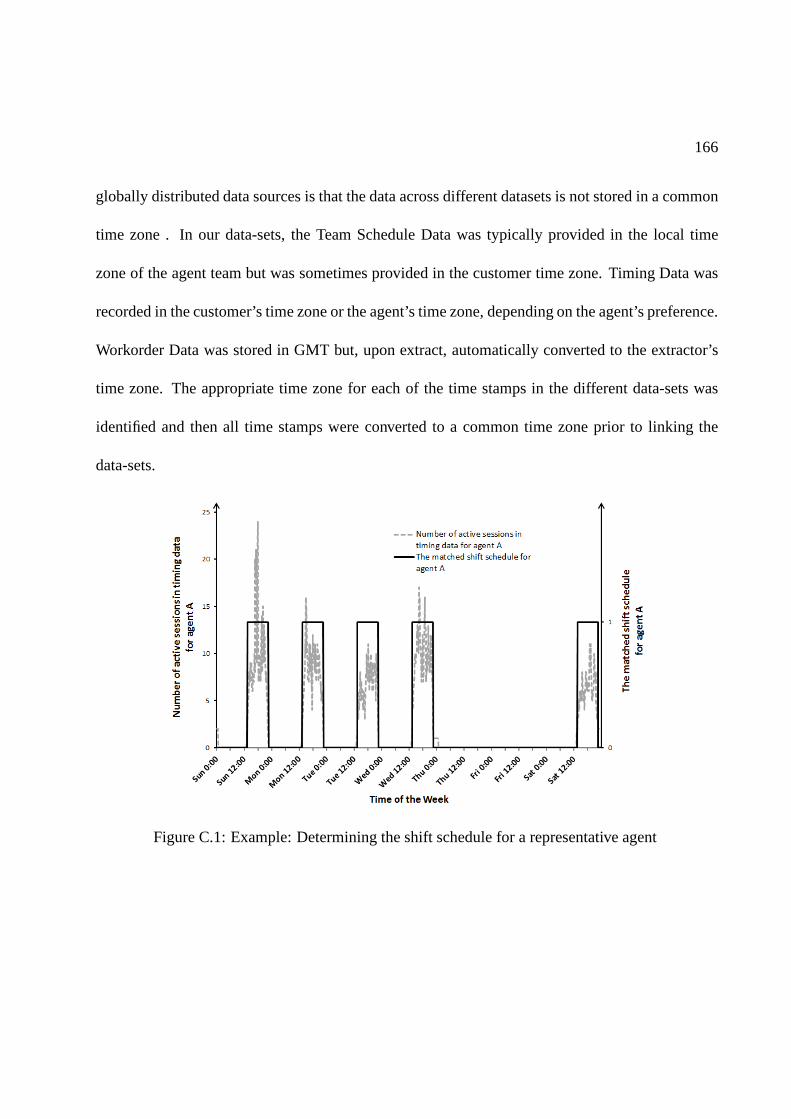
166

globally distributed data sources is that the data across different datasets is not stored in a common

time zone . In our data-sets, the Team Schedule Data was typically provided in the local time

zone of the agent team but was sometimes provided in the customer time zone. Timing Data was

recorded in the customer’s time zone or the agent’s time zone, depending on the agent’s preference.

Workorder Data was stored in GMT but, upon extract, automatically converted to the extractor’s

time zone. The appropriate time zone for each of the time stamps in the different data-sets was

identified and then all time stamps were converted to a commontime zone prior to linking the

data-sets.

Figure C.1: Example: Determining the shift schedule for a representative agent

167

C.2 Impact of Workload on Interruptions

The results in section 4.4 indicates that when a request is suspended for a period of time before

completion, the productivity of the agent is temporarily reduced after it is revisited. This section

describes two empirical models to study the impact of workload levels on the frequency and the

length of these interruptions. We also distinguish betweenplanned workload (change type requests

which are pre-scheduled for a fixed period of time) and unplanned workload (incident requests

which are assigned dynamically).

To test if interruption frequency is impacted by the workload level, we estimate the following

fixed effect linear regression model.

yih = β1WKLDplannedih + β1WKLDunplanned

ih + αi + γh + ǫih (C.1)

In equation C.1,yit counts the number of times that an incident request is suspended before

completion for agenti during hourh. VariablesWKLDplannedih andWKLDunplanned

ih are the av-

erage planned and unplanned workload levels of agenti during hourh. Fixed effects for agents

(αi) and for hour of the day (γh) are included to control for heterogeneity. The regressionhas an

R2 of 12%, and the summary statistics and the regression coefficients are reported in table C.1.

The coefficients for both types of workload levels are not statistically significant, and a joint F test

cannot reject that both of them are zero. One reason to explain this phenomenon is that the inter-

ruptions are more commonly caused by exogenous factors thatare independent of workload levels

(for example, a request is suspended because the agent is waiting for the customer’s response as an

input).

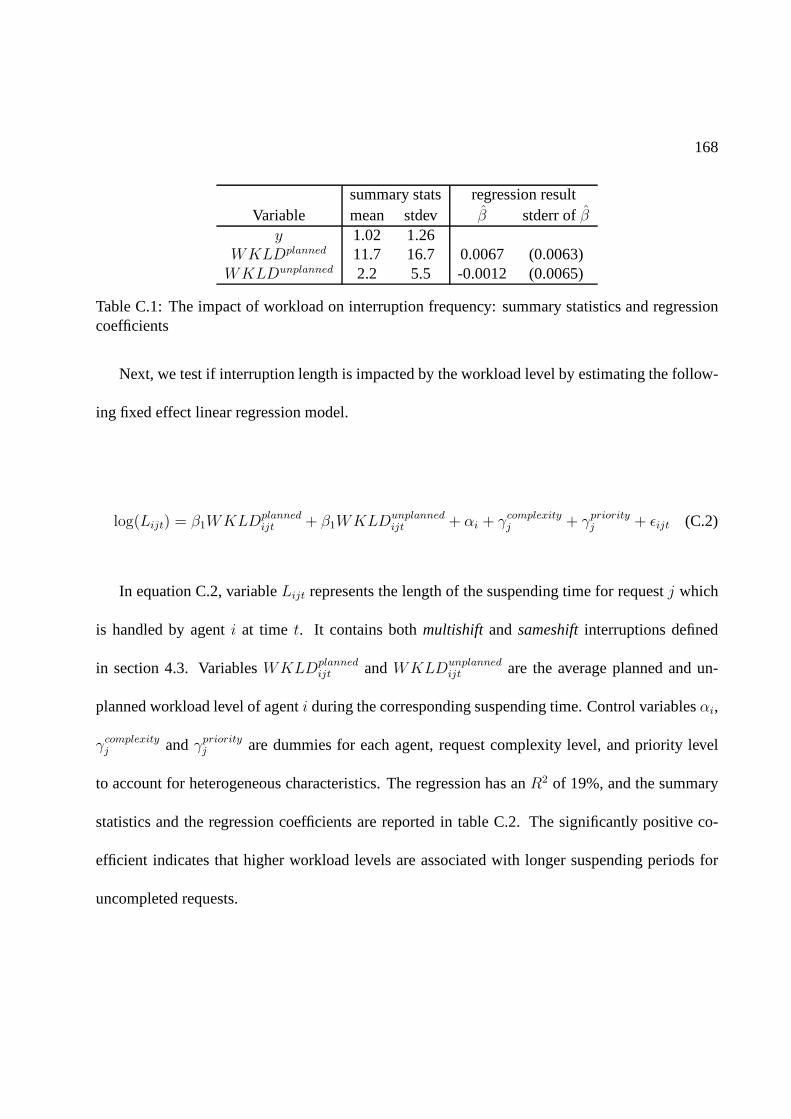
168

summary stats regression resultVariable mean stdev β stderr ofβ

y 1.02 1.26WKLDplanned 11.7 16.7 0.0067 (0.0063)WKLDunplanned 2.2 5.5 -0.0012 (0.0065)

Table C.1: The impact of workload on interruption frequency: summary statistics and regressioncoefficients

Next, we test if interruption length is impacted by the workload level by estimating the follow-

ing fixed effect linear regression model.

log(Lijt) = β1WKLDplannedijt + β1WKLDunplanned

ijt + αi + γcomplexityj + γpriorityj + ǫijt (C.2)

In equation C.2, variableLijt represents the length of the suspending time for requestj which

is handled by agenti at time t. It contains bothmultishift and sameshiftinterruptions defined

in section 4.3. VariablesWKLDplannedijt andWKLDunplanned

ijt are the average planned and un-

planned workload level of agenti during the corresponding suspending time. Control variablesαi,

γcomplexityj andγpriorityj are dummies for each agent, request complexity level, and priority level

to account for heterogeneous characteristics. The regression has anR2 of 19%, and the summary

statistics and the regression coefficients are reported in table C.2. The significantly positive co-

efficient indicates that higher workload levels are associated with longer suspending periods for

uncompleted requests.

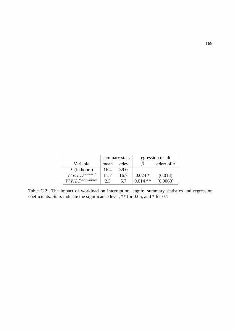
169

summary stats regression resultVariable mean stdev β stderr ofβ

L (in hours) 16.4 39.0WKLDplanned 11.7 16.7 0.024 * (0.013)WKLDunplanned 2.3 5.7 0.014 ** (0.0063)

Table C.2: The impact of workload on interruption length: summary statistics and regressioncoefficients. Stars indicate the significance level, ** for 0.05, and * for 0.1

Data-driven System Design in Service Operations System Design in Service Operations ... These...

Documents

Transcript of Data-driven System Design in Service Operations System Design in Service Operations ... These...