Data-Driven, Mechanistic and Hybrid Modelling for ... 12.pdf · Data-Driven, Mechanistic and Hybrid...

1

Data-Driven, Mechanistic and Hybrid Modelling for

Statistical Fault Detection and Diagnosis in Chemical

Processes

by:

Shallon Stubbs

A Thesis submitted in partial fulfilment of the requirements for the degree

of Doctor of Philosophy

School of Chemical Engineering and Advanced Materials

Newcastle University

United Kingdom

November, 2011

i

Abstract

Research and applications of multivariate statistical process monitoring and fault diagnostic

techniques for performance monitoring of continuous and batch processes continue to be a

very active area of research. Investigations into new statistical and mathematical methods

and there applicability to chemical process modelling and performance monitoring is

ongoing. Successive researchers have proposed new techniques and models to address the

identified limitations and shortcomings of previously applied linear statistical methods such

as principal component analysis and partial least squares. This thesis contributes to this

volume of research and investigation into alternative approaches and their suitability for

continuous and batch process applications. In particular, the thesis proposes a modified

canonical variate analysis state space model based monitoring scheme and compares the

proposed scheme with several existing statistical process monitoring approaches using a

common benchmark simulator – Tennessee Eastman benchmark process. A hybrid data

driven and mechanistic model based process monitoring approach is also investigated. The

proposed hybrid scheme gives more specific considerations to the implementation and

application of the technique for dynamic systems with existing control structures. A non-

mechanistic hybrid approach involving the combination of nonlinear and linear data based

statistical models to create a pseudo time-variant model for monitoring of large complex

plants is also proposed. The hybrid schemes are shown to provide distinct advantages in

terms of improved fault detection and reliability. The demonstration of the hybrid schemes

were carried out on two separate simulated processes: a CSTR with recycle through a heat

exchanger and a CHEMCAD simulated distillation column. Finally, a batch process

monitoring schemed based on a proposed implementation of interval partial least squares

(IPLS) technique is demonstrated using a benchmark simulated fed-batch penicillin

production process. The IPLS strategy employs data unfolding methods and a proposed

algorithm for segmentation of the batch duration into optimal intervals to give a unique

implementation of a Multiway-IPLS model. Application results show that the proposed

method gives better model prediction and monitoring performance than the conventional

IPLS approach.

ii

Acknowledgement

I would like to first express my deepest appreciation for the supervision and guidance

offered by my academic supervisors Dr. Jie Zhang and Professor Julian Morris. Their

patience and accommodation was instrumental to arriving at this point and as done much for

my character development.

I would like to acknowledge my sponsors, BP International Ltd and the Engineering and

Physical Science Research Council (EPSRC) and express my gratitude for being made a

recipient of the Dorothy Hodgkin’s Postgraduate Award. Also a special thank you note to

my industrial supervisors and liaisons, Dr. Zaid Rawi and Dr. Ian Alleyne.

Finally, a big thank you to my parents, brothers, and sisters who have all been very

encouraging and supportive over the last four years, love you all.

iii

Table of Contents

Abstract ................................................................................................................................ i

Acknowledgement ............................................................................................................... ii

Publications ..................................................................................................................... vivi

List of Figures ................................................................................................................... vii

List of Tables ........................................................................................................................x

List of Acronyms and Abbreviations..……………………………………………………xi

Chapter 1 : Introduction ...........................................................................................................1

1.1 Background and Motivation .....................................................................................1

1.2 Aims and Objective ..................................................................................................4

1.3 Thesis Contribution ..................................................................................................5

1.4 Thesis Outline ..........................................................................................................6

Chapter 2 : Review of Linear Multivariate Statistical Monitoring Techniques .......................9

2.1 Introduction ..............................................................................................................9

2.2 Principal Component Analysis ...............................................................................11

2.3 Partial Least Squares .............................................................................................17

2.4 Monitoring Metrics: Hotelling’s T2 and Q Statistics ..............................................20

2.5 Multiblock and Multiway PCA/PLS methods and Interval PLS (IPLS) ...............27

2.5.1 Multiblock Partial Least Squares .......................................................................27

2.5.2 Multiway PLS and PCA ....................................................................................28

2.5.3 Interval Partial Least Squares ................................................................................30

2.6 Dynamic PCA and PLS ..........................................................................................31

2.7 Summary ................................................................................................................33

Chapter 3 : Review of Subspace, Non-linear and Hybrid Modelling Techniques .................34

3.1 Introduction ............................................................................................................34

3.2 Canonical Variate Analysis and State Space Approach ........................................35

3.2.1 Canonical Variate Analysis ................................................................................36

3.2.2 State Space Modelling ....................................................................................38

3.2.3 State Vector Derivation ..................................................................................39

3.2.4 Stochastic estimation of the state space matrices ...........................................42

3.3 N4SID and MOESP ...............................................................................................44

3.4 Model order selection and past and future vector lag sizing ......................................51

3.4.1 Akaike Information Criterion .............................................................................52

iv

3.4.2 Normalized Residual Sum of Squares ............................................................54

3.4.3 Multiple correlation coefficient ............................................................................54

3.4.4 The Overall F-Test of the loss function ................................................................55

3.4.5 The Final prediction error criterion .......................................................................56

3.4.6 The Bayesian Information Criterion ............................................................56

3.4.7 The Law of Iterated Logarithms Criterion ...................................................57

3.5 Nonlinear Extension to PCA and PLS ...................................................................57

3.5.1 Nonlinear PCA (NLPCA) .....................................................................................58

3.5.2 Non-linear Projection to latent spaces (NLPLS) ...................................................61

3.5.3 Non-Linear Canonical Correlation Analysis (NLCCA)........................................63

3.6 Hybrid Data Driven/ Mechanistic Model based Approaches .................................64

3.7 Summary ................................................................................................................68

Chapter 4 : A Simplified CVA State Space Modelling Approach for Process-Monitoring

Specific Applications .............................................................................................................70

4.1 Introduction ............................................................................................................70

4.2 The CVA State Space Modified Approach ............................................................72

4.2.1 The Proposed Representation and Redefining of the Past Vector .....................72

4.2.2 Simplification of the State Matrices Derivation .................................................74

4.3 State matrix sizing and other modelling considerations.........................................78

4.4 Simulation 1: Evaluating the Proposed CVA SS model Accuracy and Predictive

Capabilities .........................................................................................................................85

4.5 Simulation 2: Fault Detection Capabilities Based on TE Simulator ......................88

4.5.1 The Tennessee Eastman Process ...........................................................................88

4.5.2 Fault Monitoring Statistics and Results ................................................................93

4.6. Conclusions .................................................................................................................99

Chapter 5 : Hybrid Model Based Approach to Process-Monitoring ...............................101

5.1 Introduction ..........................................................................................................101

5.2 The Plant, Model, and Fault Simulator ......................................................................103

5.2.1 CSTR Plant Simulator .........................................................................................103

5.2.2 The CSTR Simulator with Model Plant Mismatch .............................................106

5.3. Exploring Data Driven and Hybrid Model based Approaches ............................109

5.4 Performance Comparison of Mechanistic and Hybrid Fault Detection Monitoring

Schemes ............................................................................................................................121

5.4.1 The Fault Simulations .........................................................................................121

5.4.2 Fault Detection ....................................................................................................125

v

5.5 Distillation column, hybrid model, and disturbance overview ................................134

5.6 Hybrid Model Development and Fault Detection Scheme ......................................137

5.7 Impact Analysis and Detection of Simulated Disturbances .....................................140

5.7.1 Feed Temperature Change .................................................................................140

5.7.2 Feed Composition Change .................................................................................142

5.7.3 Change in Feed Flow Rate .................................................................................144

5.7.4 Combine fault Detection ....................................................................................145

5.8 Conclusions .............................................................................................................147

Chapter 6 : Batch Process Monitoring Using Multi-way and Interval PLS methods .....149

6.1 Introduction ..........................................................................................................149

6.2. Combining Data Unfolding and Interval Splicing Techniques ............................151

6.2.1 Three-dimensional data unfolding ......................................................................151

6.2.2 A binary dividing search algorithm approach for subdivision length selection ..153

6.3 Fed-batch penicillin simulator prediction and fault monitoring.................................160

6.3.1 Fed-batch Penicillin Production Process Simulator Overview ........................160

6.3.2 Prediction and Process Monitoring ..................................................................163

6.4 Prediction and Monitoring Results .............................................................................167

6.4.1 Predictive Model Performance of MiPLS Approach .......................................167

6.4.2 Process Monitoring Performance .....................................................................169

6.5 Conclusion ............................................................................................................173

Chapter 7 : Conclusions and Suggestions for Further Works .........................................174

7.1 Conclusions ..........................................................................................................174

7.2 Suggestions for Further Works ............................................................................177

Appendix A .........................................................................................................................180

Appendix B ........................................................................................................................191

References ……………………………………………………………………………….. 194

vi

Publications

Stubbs, S., J. Zhang, and J. Morris (2009), Fault detection of dynamic processes using a

simplified monitoring-specific CVA state space approach, 19th

European Symposium on

Computer Aided Process Engineering – ESCAPE19, Krakow, Poland.

Stubbs, S., J. Zhang, and J, Morris (2010), A Revised State Space Modelling Approach and

Improved Fault Detection Using Combined Index Monitoring for Dynamic Processes, 9th

International Symposium on Dynamics and Control of Process Systems - DYCOPS, Leuven,

Belgium.

Stubbs, S., J. Zhang, and J. Morris (2011), Fault detection of dynamic processes using a

simplified monitoring-specific CVA state space approach, Journal of Computers and

Chemical Engineering. (Accepted subject to minor revisions)

Stubbs, S., J. Zhang, and J. Morris (2011), Multiway Interval Partial Least Squares and a

Novel Algorithm for Optimal Interval Splicing, Journal of Chemometrics and Intelligent

Laboratory Systems. (Review Pending)

vii

List of Figures

Figure 2.1 Decomposition of the data matrix X into a collection of scores and loadings

………………………………………………………………………………15

Figure 2.2 Example plot of an SPE and T2

Monitoring on three different data sets of

historical data collected during different periods of process operation. (Stubbs, 2007) ........24

Figure 2.3 SPE contribution chart of a PCA model developed for monitoring of catalyst

production plant (Excerpt from MSc. Thesis – Stubbs, 2007) ...............................................26

Figure 2.4 Time-mode Unfolding ......................................................................................28

Figure 2.5 Batch-mode Unfolding .....................................................................................29

Figure 2.6 Variable-Mode Unfolding ................................................................................29

Figure 2.7 Unfolding of site level (batch) data. (Cherry and Qin., 2006) ..........................30

Figure 3.1 Comparing the subspace development algorithm stage of N4SID, MOESP, and

CVA………… .......................................................................................................................45

Figure 3.2 The polygonal line algorithm ............................................................................60

Figure 3.3 Architecture of neural network used to implement NLCCA. Hsieh (2001)......63

Figure 3.4 Model based PCA .............................................................................................65

Figure 3.5 Super-model based PCA ...................................................................................67

Figure 4.1 a) 3-D plot of model error vs. state vector and lag window sizes; b) Equivalent

2-D family of plots for different lag size L - MSE versus state vector dimension. ...............80

Figure 4.2 Plots of the AIC, BIC, LILC criteria dissected in terms of model complexity

term and model fitness term ...................................................................................................84

Figure 4.3 Autocorrelation plots of the output residuals ABG state space model .............86

Figure 4.4 Autocorrelation plots of the output residuals ABCDG state space model. ......87

Figure 4.5 Reconstruction of outputs for both CVA State Space models ..........................87

Figure 4.6 Histogram plot of the output residual distribution for both CVA SS models ...88

Figure 4.7 Diagram of the Tennessee Eastman process simulator under Lyman and

Georgakis control scheme. (Lyman and Georgakis, 1995) ....................................................89

Figure 4.8 AIC and NRSS computation for the monitoring-specific SS models (ABG)

spanning lag size from 1 to 5 and state order from 10 to 50. .................................................91

Figure 4.9 BIC and LLIC computation for the monitoring-specific SS models (ABG)

spanning lag size from 1 to 5 and state order from 10 to 50. .................................................92

Figure 4.10. Fault detection delay time comparison of the 5 monitoring statistics across the

2 CVA state space models. Missing bars indicate zero detection delay time, negative bars

indicate false alarm condition and full length bars indicate failed/missed detections. ..........95

Figure 4.11 Detection of fault No. 15 using ABG and ABCDG state space models ..........96

Figure 4.12 Fault detection performance of the Hotelling’s T2 statistics on the output

residuals (ABG model)...........................................................................................................97

Figure 5.1. Continuous Stirred Tank Reactor CSTR with recycle loop via Heat Exchanger

HTX…………. .....................................................................................................................104

Figure 5.2 Plant vs Mechanistic Model Outputs for different size plant-model mismatch

error…………. .....................................................................................................................108

Figure 5.3 Mismatch index plot monitoring for four different level of plant-model

mismatch……. .....................................................................................................................109

viii

Figure 5.4 Mechanistic Model-Plant interfacing options along with compensation data

driven model (a) Traditional Mechanistic Model-Plant interface (b) Proposed mechanistic-

plant interface. ......................................................................................................................110

Figure 5.5 Plant-model offset in controller output (manipulated variables) due to

mechanistic model implementation approach of Figure 5.7(a). ...........................................111

Figure 5.6 Data-based compensation model employing delayed feedback output of the

plant and mechanistic model ................................................................................................113

Figure 5.7 Mechanistic (left pane) versus PLS1 hybrid (right pane) one-step ahead

prediction of plant measured variables. Mechanistic implementation of Figure 5.4(a)

employed……. .....................................................................................................................115

Figure 5.8 Mechanistic (left pane) vs PLS1 hybrid (right pane) prediction of plant

measured variables. Mechanistic implementation of Figure 5.4(b) employed. ...................116

Figure 5.9 NRSE plots per output for hybrid model alternatives....................................119

Figure 5.10 NN Hybrid model HM2 and uncompensated mechanistic model normal

probability plot on residuals .................................................................................................119

Figure 5.11 Simulated perturbations of CSTR input variables with additive noise. ..........120

Figure 5.12. Plant overview showing unit operation faults Fp and sensor faults Fs within

and outside the process control loop. ...................................................................................121

Figure 5.13 (a) Incipient fault - Product Stream Pipe Blockage (b) Incipient faults – Cool-

water (CW) valve sticking....................................................................................................123

Figure 5.14 Fault Detection Performance of Mechanistic Model (non-hybrid approach)

using a Q statistics monitoring index. ..................................................................................126

Figure 5.15 (a) The impact of the heat exchanger fouling fault on the measured process

variables and mechanistic model output (b) The gradual decline in the magnitude of the

squared residual after the fault is initiated. ..........................................................................127

Figure 5.16 Heat exchanger fouling fault impact and detection via hybrid mechanistic –

data driven model .................................................................................................................128

Figure 5.17 Fault detection monitoring using Q statistic applied to the residuals of the 4

different hybrid model variants. ...........................................................................................129

Figure 5.18 Detection of recycle pipe blockage fault using Q, T2 and combine index

monitoring statistics on the hybrid HM3 model. .................................................................130

Figure 5.19 Detection of reactor level sensor drift using Q, T2, and combine index

statistics on the hybrid HM3 model. ....................................................................................131

Figure 5.20 Fault Magnitudes at the point of detection for the Q-statistics of the four

hybrid models.133

Figure 5.21 Dynamic Distillation Column with feed composition and condition switch

implementation .....................................................................................................................135

Figure 5.22 Hybrid data driven model architecture comprising an ANN and an OLS

model. One network is developed for each output variable. ................................................138

Figure 5.23 Complete multi-network hybrid data driven model base monitoring scheme

……………… ......................................................................................................................139

Figure 5.24 Training data profile of some of the process variable measurements used as

input and output of the hybrid data driven base process performance monitoring scheme .140

Figure 5.25 Impact of feed temperature change on distillate stream (a) flow rate plot

(b) temperature plot. .............................................................................................................141

Figure 5.26 Detection of feed temperature disturbance using T2 and Q statistics ..........142

ix

Figure 5.27 Impact of feed composition change on composition of top product. ...........142

Figure 5.28 Impact of feed composition change on distillate stream (a) flow rate plot

(b) temperature plot. .............................................................................................................143

Figure 5.29 PCA based T2 and Q Statistics detection of composition disturbance. .......144

Figure 5.30 (a) Impact of feed flow disturbance based on the distillate steam flow rate

(b) Detection of the feed flow rate disturbance using T2 and Q statistics. ...........................145

Figure 5.31 Distillate stream process variable profiles before and after feed flow-rate and

temperature change (a) Temperature (b) Mass flow-rate. ....................................................146

Figure 5.32 T2 detection of simultaneous fault conditions – (i) temperature and flow rate

change (ii) Temperature and composition change. ..............................................................147

Figure 6.1 a) Time Unfolding b) Batch-mode Unfolding..............................................152

Figure 6.2 Batch-wise interval segmented unfolding of data set. ..................................153

Figure 6.3 Flowchart of binary interval splitting algorithm .........................................154

Figure 6.4 Illustrative example of binary division algorithm for interval splitting .......155

Figure 6.5 Plot of predicted response versus actual response through different stages of

the interval splitting algorithm for case 1 with Smin = 15. ....................................................160

Figure 6.6 Flow sheet of Penicillin Cultivation Process ...............................................161

Figure 6.7 PLS2 and PLS1 implementation of a) Predictive model b) Fault monitoring

model………… ....................................................................................................................163

Figure 6.8 Plot comparing prediction of Penicillin and Biomass concentration using

online measurements a) Standard PLS model b) proposed MiPLS model ..........................168

Figure 6.9 Plot of root-mean square error RMSE reduction with discovery of the

intervals ................................................................................................................................168

Figure 6.10 Impact of a 50% step decrease in substrate feed rate (Fault #2) on a) Biomass

concentration b) Penicillin Concentration ............................................................................169

Figure 6.11 Detection of sudden faults 1 through to 3 using T2 and SPE statistics ........170

Figure 6.12 Detection of incipient faults 1 and 2 using Hotelling’s T2 statistics ............171

Figure 6.13 Detection of incipient Fault # 2 using T2 statistics a) Fault initiated at t = 50h

b) Fault initiated at t = 100h c) Fault initiated at t = 200h ...................................................172

Figure A.1 Canonical Variate Analysis (CVA) state space script layout .………...… 181

Figure A.2 CSTR plant-model mismatch coding chart ……………………………… 182

Figure A.3 Code chart outline of binary dividing segment length search algorithm… 183

Figure B.1 Interpretation of the orthogonal projection in the j-dimensional space (j = 2 in

this case) …………………………………………………………………………………..192

Figure B.2 Interpretation of the oblique projection in the j-dimensional space (j = 2 in

this case) …………………………………………………………………………………..193

x

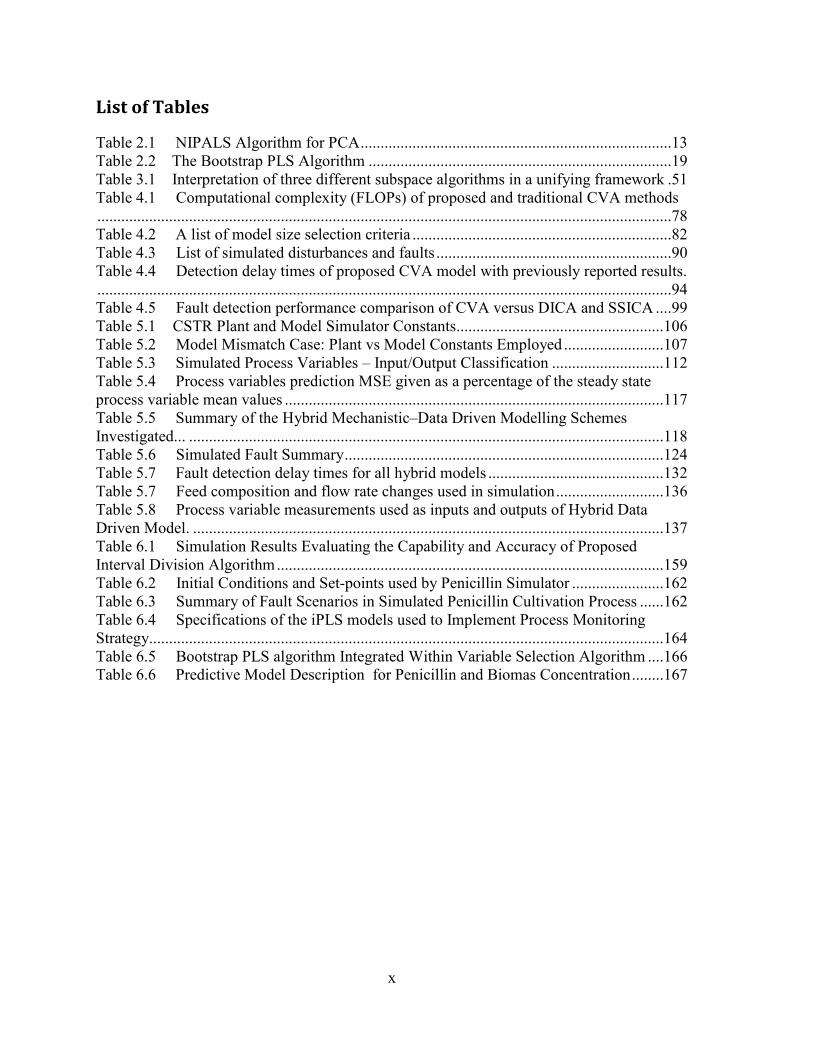
List of Tables

Table 2.1 NIPALS Algorithm for PCA ..............................................................................13

Table 2.2 The Bootstrap PLS Algorithm ............................................................................19

Table 3.1 Interpretation of three different subspace algorithms in a unifying framework .51

Table 4.1 Computational complexity (FLOPs) of proposed and traditional CVA methods

................................................................................................................................................78

Table 4.2 A list of model size selection criteria .................................................................82

Table 4.3 List of simulated disturbances and faults ...........................................................90

Table 4.4 Detection delay times of proposed CVA model with previously reported results.

................................................................................................................................................94

Table 4.5 Fault detection performance comparison of CVA versus DICA and SSICA ....99

Table 5.1 CSTR Plant and Model Simulator Constants ....................................................106

Table 5.2 Model Mismatch Case: Plant vs Model Constants Employed .........................107

Table 5.3 Simulated Process Variables – Input/Output Classification ............................112

Table 5.4 Process variables prediction MSE given as a percentage of the steady state

process variable mean values ...............................................................................................117

Table 5.5 Summary of the Hybrid Mechanistic–Data Driven Modelling Schemes

Investigated... .......................................................................................................................118

Table 5.6 Simulated Fault Summary ................................................................................124

Table 5.7 Fault detection delay times for all hybrid models ............................................132

Table 5.7 Feed composition and flow rate changes used in simulation ...........................136

Table 5.8 Process variable measurements used as inputs and outputs of Hybrid Data

Driven Model. ......................................................................................................................137

Table 6.1 Simulation Results Evaluating the Capability and Accuracy of Proposed

Interval Division Algorithm .................................................................................................159

Table 6.2 Initial Conditions and Set-points used by Penicillin Simulator .......................162

Table 6.3 Summary of Fault Scenarios in Simulated Penicillin Cultivation Process ......162

Table 6.4 Specifications of the iPLS models used to Implement Process Monitoring

Strategy.................................................................................................................................164

Table 6.5 Bootstrap PLS algorithm Integrated Within Variable Selection Algorithm ....166

Table 6.6 Predictive Model Description for Penicillin and Biomas Concentration ........167

xi

List of Abbreviations and Acronyms

Symbol Description

ABCDG 5 Matrices State Space Representation

ABG 3 Matrices State Space Representation

AIC Akaike Information Criterion

ANN Artificial Neural Network

BIC Bayesian Information Criterion

BR Balanced Realisation

BTPLS Box-Tidwell transformation based partial least squares

CA Correspondence Analysis

CCA Canonical Correlation Analysis

CCR Canonical Correlation Regression

cov Covariance

CSTR Continuous Stirred Tank Reactor

CUSUM Cumulative Sum (Statistic Monitoring Chart)

CVA Canonical Variate Analysis

CW Cool Water

DICA Dynamic Independent Component Analysis

DPCA Dynamic Principal Component Analysis

DPLS Dynamic Partial Least Squares

EWMA

Exponentially Weighted Moving Average (Statistic Monitoring

Chart)

FLOPS Floating point operations

FPE Final Prediction Error (criterion)

FTIR mid-infrared spectrum

GA Genetic Algorithm

GSVD Generalized Single Value Decomposition

HANN Hybrid Artificial Neural Network

IID Identically Identically Distributed

iPLS Interval Partial Least Squares

LILC Law of Iterative Logarithms Criterion

MBPLS Multiblock Partial Least Squares

MIMO Multiple Input Multiple Output

MiPLS Multi-way Interval Partial Least Squares

MOESP Multiple Output Error State Space

MPLS Multiway Partial Least Squares

MSE Mean Squared Error

MSPC Multivariate Statistical Process Control

xii

N4SID Numerical Algorithms for Subspace State Space System

Identification

NIPALS Non-linear Iterative Partial Least Square

NIR Near infrared spectrum

NLCCA Non-linear canonical correlation analysis

NLPLCA Non-linear Principal Component Analysis

NLPLS Non-linear Partial Least Squares

NN Neural Network

NRSS Normalized Residual Sum Squares

OLS Ordinary Least Squares

OVF Overall F-test of the loss function (criterion)

PCA Principal Component Analysis

PENSIM

Fed-batch Penicillin Fermentation Simulator (Birol, et al.,

2002)

PLS Partial Least Squares

PLS1 Single-Block PLS

PLS2 Two-Block PLS

PLSR Partial Least Squares Regression

QPLS Quadratic Partial Least Squares

RMSE Root Mean Square Error

SPC Statistical Process Control

SPE Square Prediction Error or Q Statistics

SS State Space

SSICA State Space Independent Component Analysis

SVD Single Value Decomposition

TE Tennessee Eastman (Simulator)

TSS Total Sum of Squares

1

Chapter 1 : Introduction

1.1 Background and Motivation

Two separate advances, one in sensing technology and data acquisition system and the other in

process modelling software has revolutionized the chemical process industry in aspects ranging

from plant design, implementation, monitoring and controls. The control strategies have become

more complex and more model-based strategies are being explored as the drive to be more

efficient, globally competitive and environmentally friendly continues to impose upon

production facilities tighter safety and product quality operating constraints. Engineers, plant

managers, and operators are becoming increasingly aware of the unlocked potential of the

volume of measurement data that is sampled and stored in computer archives. With more

complex plants and operating constraints, more efforts are being utilized to extract as much

information and understanding from the process data gathered by the various plant sensors. The

ultimate objective is that such acquired knowledge and insight into the plant dynamics can be

translated into improved plant performance monitoring and control schemes.

There is also the growing curiosity about extracting more usefulness from chemical process

modelling software beyond plant design or feasibility and pinch analysis evaluation. To that end

advances in chemical modelling software continue to seek to provide more user-friendly

development environment for more robust and accurate dynamic models that can be employed as

engines in model-based control systems or for the purposes of online process monitoring and

quality variable prediction.

2

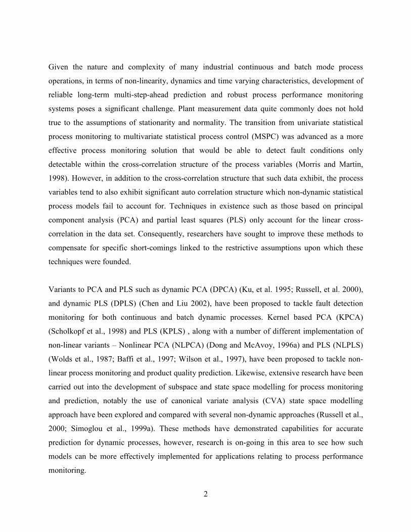
Given the nature and complexity of many industrial continuous and batch mode process

operations, in terms of non-linearity, dynamics and time varying characteristics, development of

reliable long-term multi-step-ahead prediction and robust process performance monitoring

systems poses a significant challenge. Plant measurement data quite commonly does not hold

true to the assumptions of stationarity and normality. The transition from univariate statistical

process monitoring to multivariate statistical process control (MSPC) was advanced as a more

effective process monitoring solution that would be able to detect fault conditions only

detectable within the cross-correlation structure of the process variables (Morris and Martin,

1998). However, in addition to the cross-correlation structure that such data exhibit, the process

variables tend to also exhibit significant auto correlation structure which non-dynamic statistical

process models fail to account for. Techniques in existence such as those based on principal

component analysis (PCA) and partial least squares (PLS) only account for the linear cross-

correlation in the data set. Consequently, researchers have sought to improve these methods to

compensate for specific short-comings linked to the restrictive assumptions upon which these

techniques were founded.

Variants to PCA and PLS such as dynamic PCA (DPCA) (Ku, et al. 1995; Russell, et al. 2000),

and dynamic PLS (DPLS) (Chen and Liu 2002), have been proposed to tackle fault detection

monitoring for both continuous and batch dynamic processes. Kernel based PCA (KPCA)

(Scholkopf et al., 1998) and PLS (KPLS) , along with a number of different implementation of

non-linear variants – Nonlinear PCA (NLPCA) (Dong and McAvoy, 1996a) and PLS (NLPLS)

(Wolds et al., 1987; Baffi et al., 1997; Wilson et al., 1997), have been proposed to tackle non-

linear process monitoring and product quality prediction. Likewise, extensive research have been

carried out into the development of subspace and state space modelling for process monitoring

and prediction, notably the use of canonical variate analysis (CVA) state space modelling

approach have been explored and compared with several non-dynamic approaches (Russell et al.,

2000; Simoglou et al., 1999a). These methods have demonstrated capabilities for accurate

prediction for dynamic processes, however, research is on-going in this area to see how such

models can be more effectively implemented for applications relating to process performance

monitoring.

3

The developments of simple process faults often propagate into complex faults due to process

feed recycle loops and control system feedback. The control system may also conceal the

development of the fault depending upon the nature of the fault and its impact on the process.

Developing better understand of the impact such control loops have on the detection and

development of faults is one avenue by which existing fault monitoring schemes could be

enhanced. It is the author’s view that in deriving and developing better statistical models for

monitoring, not only the statistical nature of the process data but also other aspects specific to the

design and operation of industrial processes should be taken into consideration. Such work will

hopefully help resolve some of the conflict that sometimes appears to exist between process

controls and process monitoring systems. Process control and predictive modelling should be

able to co-exist with statistical process monitoring, each providing support and coordinating with

the other.

The statistical data based models for monitoring is significantly more prevalent than mechanistic

first principle models because of the time, process knowledge and overall cost involved in

developing robust and reliable mechanistic models, particular for large plants characterized by

complex and non-linear dynamics. The main advantage that the mechanistic model approach

may provide over data driven models is the ability to incorporate process knowledge into the

model design. With the models being based upon actual chemistry and design parameters of the

process, it may prove more effective in capturing the relevant process dynamics and non-linear

features characterizing the operation of plant, thus enabling more reliable and robust model for

process monitoring application. Reported advances in software development packages,

particularly in the area of dynamic online models, have made such endeavours more feasible.

However, the question of whether it is possible to produce robust and sufficiently reliable model

based on limited process information and or imprecise data with uncertainty is the more pertinent

issue that also needs to be taken into consideration.

The two approaches have contrasting strengths and weaknesses which should be weighed against

each in order for one method to be declared better than the other. Case in point, if the

mechanistic fault monitoring approach is capable of yielding better detection and diagnostic

improvements over a statistical data driven method, is the improvements significant enough to

4

warrant the additional effort in developing such models? Or perhaps one may want to consider

whether the fusion of the two approaches could be orchestrated to complement each other and

yield a superior hybrid process monitoring scheme.

Mcpherson (2007) explored several hybrid schemes in her doctoral research thesis, the schemes

analysed used PCA, CVA, NLPCA, autoregressive with exogenous input (ARX) time series

model combined with mechanistic models of a batch process to monitor several different types of

simulated faults. The analysis, however, does not include the application of hybrid approaches

involving the merger of different statistical data driven methods or the comparative performance

of pure data driven or pure mechanistic approaches for process performance monitoring.

1.2 Aims and Objective

The main goal of this research is to provide novel statistical modelling solutions and or

enhancements to existing methods that will improve the reliability, speed of fault detection, and

scope of application for model based process monitoring and fault diagnostics systems. More

specifically, the following objectives will be sought to be achieved:

i) Discovering statistical methods and design methodologies for improving dynamic

modelling approaches. The success of any proposed method to be evaluated via

comparative analysis with pre-existing approaches.

ii) Development of hybrid approaches involving the combination of mechanistic

(first principle models) and statistical linear and or non-linear data driven

methods. Specific consideration will be given to implementation, the impact of

mechanistic model-plant mismatches on the performances of such system, the

choice of data based model and performance improvement over traditional non-

hybrid data driven approaches.

iii) Development of hybrid data based models employing both linear and non-linear

statistical data driven methods for applications where the cost of development of a

mechanistic model is prohibitive or the chemistry and dynamics of the system are

not well defined.

iv) Improving predictive modelling and fault monitoring of batch processes

characterized by nonlinearity and significant inter-batch variation.

5

1.3 Thesis Contribution

The thesis contributes both investigatory research expanding upon evaluation and analysis

carried out by previous researchers and also proposes several novel approaches to fault detection

model development and detection monitoring metrics for both continuous and batch process

performance monitoring. The key contributions are summarized as follows:

� An amendment to the traditional canonical variate analysis state space model

development process is proposed that leads to a simpler monitoring scheme. The model’s

simplification is demonstrated via the reduction in the model parameterization

dimensions and the computationally simpler algorithms required for parametric

estimation. The fault detection performance capabilities of the proposed model is

compared with several other traditional statistical models such as PCA, DPCA,

correspondence analysis (CA), and the Larimore’s CVA state space model

implementation. The results indicate that the fault detection performance of the proposed

model is not compromised by the simplification achieved.

� A central aim of this research was to investigate the employment of hybrid modelling

architecture for process performance monitoring endeavours. The hybrid schemes

investigated in this thesis involved mechanistic (first principle) models and data driven

statistical models as well as combining statistical data driven approaches of different

types. To justify the need for the proposed hybrid approaches or the role of the data based

compensation model, the fault detection and process performance monitoring hybrid

schemes were evaluated and compared against an approach based on a mechanistic based

only system. A non-mechanistic hybrid scheme implementation combining an ordinary

least squares (OLS) and neural network based model is proposed and evaluated as a

solution to large scale plant monitoring applications characterized by nonlinear variability

due to operating point fluctuations.

� Finally, multi-way data unfolding method was combined with interval partial least

squares (iPLS) to provide an improved linear approximation model of a highly non-linear

batch penicillin production process. An algorithm for deriving the optimal lengths of the

6

intervals to be employed was developed by the author and demonstrated to give very

consistent results. Multiway interval partial least squares (MiPLS) models were

developed for both quality variable prediction and fault detection.

1.4 Thesis Outline

The remaining part of the thesis is organised as follows. Chapter 2 summarizes and provides

succinct description of some of the linear multivariate statistical process monitoring approaches

that have been reported in the literature. The review spans a wide range of research commencing

with an overview of PCA and PLS. The coverage will expand to the several extensions of these

methods, namely multi-way and multi-block PCA and PLS, and a more recent evolution in PLS

modelling – interval partial least squares.

Chapter 3 extends the literature review focusing on dynamic and non-linear extension to the

linear statistical models introduced in Chapter 2. The coverage will include DPCA and DPLS,

and other subspace projection methods will also be discussed such as CVA state space models

and so forth. With regards to the nonlinear models, the chapter will review nonlinear principal

component analysis (NLPCA) and nonlinear partial least squares (NLPLS) along with a dynamic

nonlinear canonical correlation analysis (CCA) approach. The chapter also gives an overview of

several hybrid mechanistic – data driven model approaches that have been previously proposed

in literature.

.

Chapter 4 presents the author’s investigation into CVA state space modelling for dynamic

process monitoring and modelling. A variant to the traditional CVA state space model is

presented and both the proposed and traditional CVA state space modelling approach were

dissected revealing the significant gains in computational simplicity achieved via use of a

simpler state space representation and estimation algorithms employed by the proposed model.

The performance results of the models will be evaluated on the Tennessee Eastman process

simulator and compared against other statistical projection techniques such as (D)PCA and

correspondence analysis CA. Results obtain from a second case study based upon process

monitoring of a distillation column model will also be reported.

7

In Chapter 5, several hybrid modelling schemes for process monitoring are proposed and

analyzed. For the proposed mechanistic-data driven hybrid scheme specific consideration are

given to the implementation and monitoring of process plants under close-loop controls. The

chapter explores implementation issues with regards to defining the interface between the

mechanistic model and the actual plant. The impact of model plant mismatches is also explored

and the capabilities of the data based model to compensate for such. The fault detection and

monitoring performance of several proposed hybrid architectures are analyzed. The hybrid model

based performance monitoring schemes were evaluated using a continuous stirred tank reactor

CSTR – heat exchanger recycle loop simulator which has been employed in previous research

work (Zhang, 2006; Zhang, et al., 1996). An alternative hybrid scheme based on combining a

nonlinear and linear statistical data base model is also proposed as a means of developing a

pseudo time-variant model for a distillation column process simulator.

The results reported in the chapter demonstrate the feasibility of both proposed hybrid schemes.

More specifically it provides evidence that both the prediction and fault detection performance of

a mechanistic model-based monitoring scheme can be enhanced by compensating the model with

a data-driven model.

In Chapter 6 the focus is shifted to addressing quality variable prediction and performance

monitoring of non-linear batch processes using a monitoring strategy that merges both three

dimensional data unfolding techniques proposed by Wold et al. 1987 with an emerging partial

least squares modelling technique referred to as interval partial least squares iPLS. The multiway

iPLS (MiPLS) model development employs a novel algorithm, described in the chapter, for

partitioning of the intervals used by the model. The MiPLS model’s quality variable prediction

and overall batch monitoring performance is demonstrated to be superior to the standard PLS

model-based approach. The well-known penicillin fermentation simulator developed and

enhance by researchers out of Illinois Institute of Technology (Birol, et al. 2002) was employed

for evaluating the predictive and process monitoring capable of the proposed model.

8

Chapter 7 closes with a summary overview on the various statistical and mechanistic model-

based approaches explored in the research, highlighting the main conclusions from key results

obtained. The scope of potential future research in the area is also discussed.

9

Chapter 2 : Review of Linear Multivariate Statistical Monitoring

Techniques

2.1 Introduction

The major limitation of traditional univariate statistical process control (SPC) for process

performance monitoring, as pointed out by Martin et al. (1996) , is the independent basis by

which each process variable is monitored to identify developing faults. The detection and

diagnosis of malfunctions may in such case be impaired by this limitation. Firstly, due to the fact

that the select monitored variables are not necessarily independent and hence faults due to

multivariate correlated occurrences may go undetected. And secondly, in the case of large

complex plant set up, the large number of sensor measurement sampled on a 24 hour basis can

easily overwhelm such an approach. Multivariate SPC (MSPC) is an extension of univariate

SPC where the correlation between process quality variables and process variables are taken into

consideration.

MSPC methods unlike its univariate counterpart are capable of detecting malfunctions that are

due to correlated events and events that are not detected readily by magnitude deviations in

independently monitored quality variables. MSPC is based mainly on projection methods that

seeks to extract the correlation in variability among a set of simultaneously measured process

variables and or to quantify the extent to which such variability and correlation structure may be

linked to observable trends in one or more process quality variables. The two most common

projection methods are PCA and PLS (MacGregor et al., 1991) .

PCA is a data dimension reduction technique that exploits the correlations among the vast

amounts of plant measurement data collected (Jolliffe, 2002; Wold, et al., 1987). It is inherently

10

static as the projection and directional information with respect to the variability in the data at

any given time is only dependent upon the current samples and does not take into account the

possible influence of past samples on the current observation (Russell, et al., 2000).

Projection to latent structures or partial least squares seeks to simultaneously reduce the

dimensional space of the process measurement variables and process quality variables. The

method is employed in product quality prediction as PLS extracts a set of latent variables that not

only account for the variability in the process variables but are also most correlated to the

variability in the product quality variables.

During the reign of univariate SPC, the univariate monitoring of process quality variables would

involve the use of univariate statistical charts, such as CUSUM (cumulative sum) plots, EWMA

(exponentially weighted moving average) charts and Shewhart charts (MacGregor and Kourti,

1995). These charts evaluate the performance of the process by comparing them against derived

control limits determined from measurements taken when the process was known to be

conforming to the product specification limits. Similarly an essential component to MSPC is the

development of multivariate control charts to detect disturbances and fault conditions as they

may arise. Multivariate project techniques employ the same philosophy as that for univariate or

multivariate shewharts charts (MacGregor and Kourti, 1995). The multivariate Hotelling’s T2

chart and the square prediction error (SPE) or Q-Statistics chart is generated based upon of a

subset of the latent vectors used in defining the model. The main understanding and justification

of the use of such chart for monitoring can be found in Kresta et al. (1991b). The mathematics

behind such charts is described in greater detail in later subsections. Other proposed multivariate

control charts include Multivariate CUSUM charts (Healy, 1987), multivariate EWMA charts

(Lowry et al., 1991).

Recent researches have been directed at addressing and compensating for specific-shortcomings

linked to the restrictive assumptions upon which techniques such as PCA and PLS is based. That

is, the assumption that the data samples exhibit minimal auto and cross-correlation. Several

variants to the standard PCA and PLS approach have been proposed in the literature and will be

addressed in this and the following chapter.

11

The remainder of this chapter is as follows. Section 2.2 describe the projection method of PCA,

the NIPALS PCA algorithm, and theory behind identifying the reduce subspace for data

dimension reduction. Section 2.3 reviews both the single and two block PLS methods, the

various proposed PLS algorithms and discussion on their suitability for process monitoring

applications. Section 2.4 looks the two most well-known monitoring statistics – Hotelling’s T2

and Q statistics and discusses their application to process monitoring. Section 2.5 reviews the

PLS and PCA variants that have been reported in the literature which are particularly applicable

to batch processes such as Multi-way and Multi-block PLS and PCA methods. Section 2.6

reviews the dynamic extension to the standard PCA and PLS method. Section 2.7 closes the

chapter with a summary overview of the literature reviewed.

2.2 Principal Component Analysis

Principal component analysis (PCA) is a mathematical linear orthogonal transformation

technique that exploits the correlation existing among measured process variables in order to

reduce the dimensionality of the measurements. The principal component score vectors are linear

weighted sum of the original process variables. The weights associated with the process variables

for a given score/principal component computation defines the principal component score vector

and are alternately referred to as the loadings for the principal component. The loadings are

derived from the eigenvectors of the covariance matrix and as such the resulting scores are

themselves uncorrelated and hence a significantly reduce number of scores can be used to

represent the majority of the variability in the measurement variables provided that the process

variables exhibit a high degree of correlation.

PCA was first introduced by Karl Pearson in 1991 but did not really catch on in use and

popularity until advances in computing and electronics facilitated such (Jolliffe, 2002). The

methods of deriving the principal component using eigenvector decomposition or single value

decomposition (SVD) were considered computationally intensive at the time of its inception. The

method has will be shown in the following analysis is both scale and noise sensitive.

12

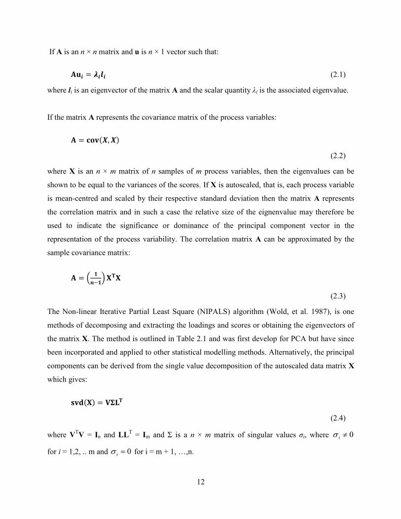
If A is an n × n matrix and u is n × 1 vector such that:

�� = �� (2.1)

where li is an eigenvector of the matrix A and the scalar quantity λi is the associated eigenvalue.

If the matrix A represents the covariance matrix of the process variables:

� = ��, �

(2.2)

where X is an n × m matrix of n samples of m process variables, then the eigenvalues can be

shown to be equal to the variances of the scores. If X is autoscaled, that is, each process variable

is mean-centred and scaled by their respective standard deviation then the matrix A represents

the correlation matrix and in such a case the relative size of the eignenvalue may therefore be

used to indicate the significance or dominance of the principal component vector in the

representation of the process variability. The correlation matrix A can be approximated by the

sample covariance matrix:

� = � ��

(2.3)

The Non-linear Iterative Partial Least Square (NIPALS) algorithm (Wold, et al. 1987), is one

methods of decomposing and extracting the loadings and scores or obtaining the eigenvectors of

the matrix X. The method is outlined in Table 2.1 and was first develop for PCA but have since

been incorporated and applied to other statistical modelling methods. Alternatively, the principal

components can be derived from the single value decomposition of the autoscaled data matrix X

which gives:

�� = ��

(2.4)

where VTV = In and LL

T = Im and Σ is a n × m matrix of singular values σi, where 0≠iσ

for i = 1,2, .. m and 0=iσ for i = m + 1, …,n.

13

The singular values are the standard deviations of the principal component scores and are hence

related to the square root of the eigenvalues of the correlation matrix A since:

�� = �Σ�� Σ��

�� = �Σ� Σ��

Post-multiplying both sides by L:

!� = ��"#$

Considering the above equation in relation to Eq. (2.1), the right-hand size matrix L and diagonal

matrix of singular values Σ maps unto the full set of eigenvectors and eigenvalues:

L = [l1, l2, ..... , lm] and �" = �%&'(�,)(", … . . , ($ (2.5)

Table 2.1 NIPALS Algorithm for PCA

0 Set t = to a column in X; set E0 = X; set threshold (e.g. , = 0.001 for convergence

check; i = 1.

1 Project X onto t to find the corresponding loading l: �/ = 0/�1� 2/ 2/�2/ 3

2 Normalize the loading vector l to unit length:

�/ = �/ 4��/5

3 Project X onto l to find the corresponding score vector t: 2/ = 0/�1� �/ ��/ 3

4 Check for convergence:

If the difference between the eigenvalues 6 78 = 2/�2/ in the current iteration is > , ∗ 6:;< then return to step 1 else move to step 5.

5 Prepare for next loadings and score vector extraction:

i = i + 1; 0/ = =/�1 − 2/�/�

14

The scores may be interpreted as the projection or mapping of the original sample measurements

unto the subspace spanned by the subset of the p selected uncorrelated principal component

vectors. Eq.(2.7) describes the linear variable transformation carried out on the m process

variables collected at the ith sample instance to compute the score projection onto the jth

principal component:

immjijijijij xlxlxlxlt +++= ..........332211

(2.6)

The principal component vector loading lkj is the coefficient associated with the kth process

variable and the jth principal component while xik, is the ith sampled measurement of the kth

process variables. The principal component scores computation of n samples using a subset of p

principal component loadings is represented in matrix form via Eq.(2.8) or diagrammatically in

Figure 2.1.

=

mpmm

p

p

nmnn

m

m

npnn

p

p

lll

lll

lll

xxx

xxx

xxx

ttt

ttt

ttt

....

....

....

.

.

.

.

..

..

...

...

...

...

..

..

21

22221

11211

21

22221

11211

21

22221

11211

(2.7)

The principal component loadings (Lp = [l1 l2 ……. lp]) are of unit length and are orthogonal as

such, if the full set or subset of principal component are used, the loading matrix pre-multiplied

by its transpose would give a p x p identity matrix:

pp

T

p ILL = (2.8)

where p <= m. Note post-multiplication does not result in an identity matrix as will be shown

later.

15

= + + .....+

Figure 2.1 Decomposition of the data matrix X into a collection of scores and loadings

The reconstruction based upon the reduce dimension subspace of principal component loadings

and computed scores is given by:

T

ppLTX =ˆ

(2.9)

The choice of the subspace dimension (p < m) usually incorporates the most significant principal

components. The common justification provided is that, the choice separates the full dimension

of principal components into two subspace with Lp subspace accounting for the structured

variability present in the measurement and the other subspace made up of the higher order

principal components accounting mostly for the unstructured noise present in the measurements

(MacGregor and Kourti, 1995).

Since Tp = XLp then:

m

T

ppˆ XPLXLX ==

(2.10)

where Pm is an m × m matrix but not necessarily an identity matrix.

In fact Pm only computes into a perfect identity matrix when the full complement or the number

of components equal to the rank order of the matrix is included in the PCA model.

�1� t1 �?� t2 X E

16

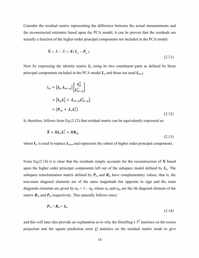
Consider the residual matrix representing the difference between the actual measurements and

the reconstructed estimates based upon the PCA model, it can be proven that the residuals are

actually a function of the higher-order principal components not included in the PCA model:

)(XX~

mm PIXX −=−=

(2.11)

Now by expressing the identity matrix Im using its two constituent parts as defined by those

principal components included in the PCA model Lp and those not used Lm-p:

�@ = A�B)�@�BC D �B��@�B� E

))))))= A�B�B� +)�@�B�@�B� C

))))))= GH@ +)�I�I�J

(2.12)

It, therefore, follows from Eq.(2.12) that residual matrix can be equivalently expressed as:

�K = ��I�I� = �L@

(2.13)

where Lr is used to replace Lm-p and represents the subset of higher order principal components.

From Eq.(2.14) it is clear that the residuals simply accounts for the reconstruction of X based

upon the higher order principal components left out of the subspace model defined by Lp. The

subspace transformation matrix defined by Pm and Rm have complementary values, that is, the

non-main diagonal elements are of the same magnitude but opposite in sign and the main

diagonals elements are given by αri = 1 – αpi where αri and αpi are the ith diagonal element of the

matrix Rm and Pm respectively. This naturally follows since:

Pm + Rm = Im

(2.14)

and this will later also provide an explanation as to why the Hotelling’s T2 statistics on the scores

projection and the square prediction error Q statistics on the residual matrix tends to give

17

complimentary detection, that is, a fault detected by one statistics may fail to be detected by the

other.

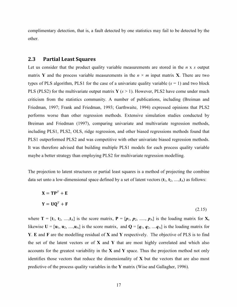
2.3 Partial Least Squares

Let us consider that the product quality variable measurements are stored in the n x s output

matrix Y and the process variable measurements in the n × m input matrix X. There are two

types of PLS algorithm, PLS1 for the case of a univariate quality variable (s = 1) and two block

PLS (PLS2) for the multivariate output matrix Y (s > 1). However, PLS2 have come under much

criticism from the statistics community. A number of publications, including (Breiman and

Friedman, 1997; Frank and Friedman, 1993; Garthwaite, 1994) expressed opinions that PLS2

performs worse than other regression methods. Extensive simulation studies conducted by

Breiman and Friedman (1997), comparing univariate and multivariate regression methods,

including PLS1, PLS2, OLS, ridge regression, and other biased regressions methods found that

PLS1 outperformed PLS2 and was competitive with other univariate biased regression methods.

It was therefore advised that building multiple PLS1 models for each process quality variable

maybe a better strategy than employing PLS2 for multivariate regression modelling.

The projection to latent structures or partial least squares is a method of projecting the combine

data set unto a low-dimensional space defined by a set of latent vectors (t1, t2, ....,tA) as follows:

� = �M� + N

O = PQ� + R

(2.15)

where T = [t1, t2, ....,tA] is the score matrix, P = [p1, p2, ....., pA] is the loading matrix for X,

likewise U = [u1, u2, ....,uA] is the score matrix, and Q = [q1, q2, ....qA] is the loading matrix for

Y. E and F are the modelling residual of X and Y respectively. The objective of PLS is to find

the set of the latent vectors or of X and Y that are most highly correlated and which also

accounts for the greatest variability in the X and Y space. Thus the projection method not only

identifies those vectors that reduce the dimensionality of X but the vectors that are also most

predictive of the process quality variables in the Y matrix (Wise and Gallagher, 1996).

18

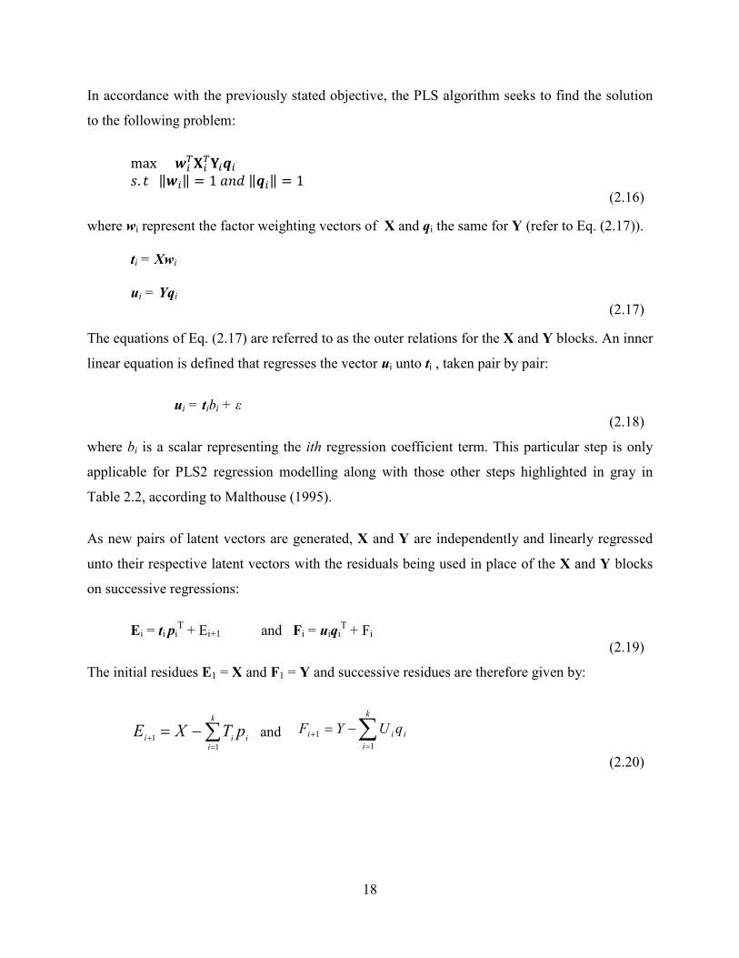
In accordance with the previously stated objective, the PLS algorithm seeks to find the solution

to the following problem:

max V/��/�O/W/ X. Y)))ZV/Z = 1)[\])ZW/Z = 1))) (2.16)

where wi represent the factor weighting vectors of X and qi the same for Y (refer to Eq. (2.17)).

ti = Xwi

ui = Yqi

(2.17)

The equations of Eq. (2.17) are referred to as the outer relations for the X and Y blocks. An inner

linear equation is defined that regresses the vector ui unto ti , taken pair by pair:

ui = tibi + ε

(2.18)

where bi is a scalar representing the ith regression coefficient term. This particular step is only

applicable for PLS2 regression modelling along with those other steps highlighted in gray in

Table 2.2, according to Malthouse (1995).

As new pairs of latent vectors are generated, X and Y are independently and linearly regressed

unto their respective latent vectors with the residuals being used in place of the X and Y blocks

on successive regressions:

Ei = ti piT + Ei+1 and Fi = uiqi

T + Fi

(2.19)

The initial residues E1 = X and F1 = Y and successive residues are therefore given by:

∑=

+ −=k

iiii

pTXE1

1 and ∑

=+ −=

k

i

iii qUYF1

1

(2.20)

19

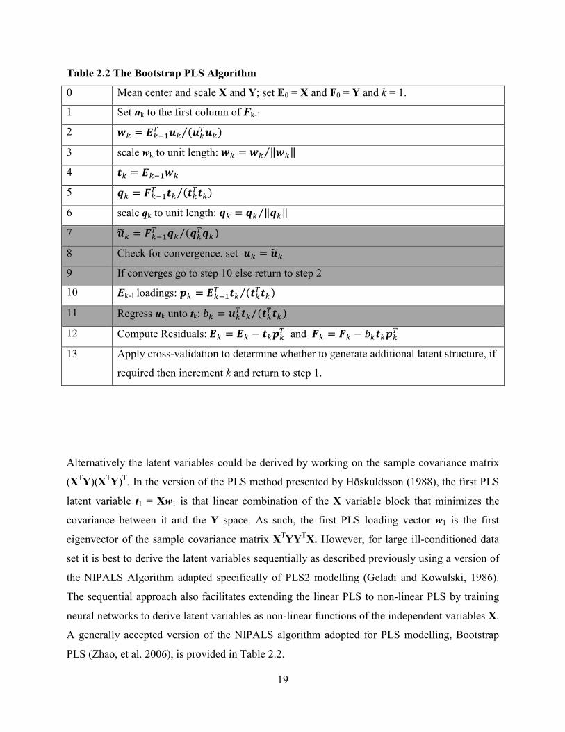
Table 2.2 The Bootstrap PLS Algorithm

0 Mean center and scale X and Y; set E0 = X and F0 = Y and k = 1.

1 Set uk to the first column of Fk-1

2 V^ = 0^�1� _^ _�_^ 3

3 scale wk to unit length: V^ = V^ ZV^Z3

4 2^ = 0^�1V^

5 W^ = `^�1� 2^ 2�2^ 3

6 scale qk to unit length: W^ = W^ ZW^Z3

7 _a^ = `^�1� W^ W�W^ 3

8 Check for convergence. set _^ = _a^

9 If converges go to step 10 else return to step 2

10 Ek-1 loadings: b^ = 0^�1� 2^ 2�2^ 3

11 Regress uk unto tk: c^ = _�2^ 2�2^ 3

12 Compute Residuals:)0^ = 0^ − 2^b� and )`^ = `^ − c^2^b�

13 Apply cross-validation to determine whether to generate additional latent structure, if

required then increment k and return to step 1.

Alternatively the latent variables could be derived by working on the sample covariance matrix

(XTY)(X

TY)

T. In the version of the PLS method presented by Höskuldsson (1988), the first PLS

latent variable t1 = Xw1 is that linear combination of the X variable block that minimizes the

covariance between it and the Y space. As such, the first PLS loading vector w1 is the first

eigenvector of the sample covariance matrix XTYY

TX. However, for large ill-conditioned data

set it is best to derive the latent variables sequentially as described previously using a version of

the NIPALS Algorithm adapted specifically of PLS2 modelling (Geladi and Kowalski, 1986).

The sequential approach also facilitates extending the linear PLS to non-linear PLS by training

neural networks to derive latent variables as non-linear functions of the independent variables X.

A generally accepted version of the NIPALS algorithm adopted for PLS modelling, Bootstrap

PLS (Zhao, et al. 2006), is provided in Table 2.2.

20

If we define the following R = [r1, r2,....., rA] as:

d1 = V1

d/ = ∏f#@ −Vgbg�hV/, i > 1

(2.21)

Then the scores matrix T can be computed directly from the original X matrix without deflation

and the final model can be expressed in closed form multiple regression type prediction model

(Dejong, 1993; Li, et al., 2010):

� = �i (2.22)

O = �jklm + R

jklm = iQ�

(2.23)

P, R, and W have the following relationship:

i = nM�n �1

(2.24)

ioM = Moi = non = #!

(2.25)

Li, et al. (2010) compared the suitability of two other proposed PLS algorithms – Weight-

deflated PLS (WPLS) (Helland, 1998) and SIMPLS (Dejong, 1993) with the standard

(established) PLS algorithm described earlier and documented in Table 2.2. The paper concluded

based upon geometric analysis of the algorithms and simulation performance results that the

standard PLS algorithm was best suited for applications involving fault detection monitoring.

2.4 Monitoring Metrics: Hotelling’s T2 and Q Statistics

The Hotelling’s T2 and squared prediction error (SPE) or Q-statistics monitoring plots and

contribution charts are quite effective multivariate control charts which can be employed in

distinguishing between the good-nominal operating plant conditions versus an abnormal plant

condition (MacGregor and Kourti, 1995). The T2 plots and SPE (Q) statistics are interlinked in

21

that they are both dependent upon the number of principal components (latent variables in the

case of PLS) chosen for inclusion.

2g = p�qV�g

(2.26)

where tj is the scores/principal component, lj is the jth loading vector or latent variables (in the

case of PLS), and xnew is the 1 × m row vector of new measurements on the process variables.

Note that there is a score vector evaluated per loading vector and represents the projection of the

variance in the original measurement variables onto that particular principal component axis.

The T2 plot is a measure of the deviation of the squared scores scaled by the eigenvalues

(variance of the scores) obtained from the PCA model developed using normal operation (NOP)

data. Eq. (2.27) evaluates the overall squared score values at the ith sample instance by summing

together the square of the A scores value representing the projection of the m process variables

unto the A dominant principal component vectors.

∑=

=A

jj

ij

i

tT

1

2

2

λ

(2.27)

Alternatively, the Hotelling’s T2 statistics on the scores can be expressed using matrix notation:

r? = )��b��"�B��

(2.28)

PLS has been used in multivariate monitoring of process is pretty much identical ways to PCA

based monitoring (Kresta, et al., 1991a). In the case of PLS, similar T2 statistics have been

proposed for monitoring using the latent vectors of X that can be conveniently be extracted using

Eq. (2.22), the Hotelling’s T2 statistics is then similarly calculated using:

2 = pstui

r? =) 2 78o v��2 78 (2.29)

where v = 1 �1�� is the sample covariance matrix of the scores.

22

In general, SPE or Q statistics plot is based upon evaluating the summation of the square

difference or squared residuals between actual process variable measurements and that of the

reconstructed estimates of the said:

2

,1

,)ˆ(

inew

m

iinew

xxSPE −= ∑=

where T

AnewAnewPTX

,ˆ =

(2.30)

In the case of PCA the estimation �w can be derived using Eq. (2.9) or (2.10) and the residuals �K = � − �w can be alternatively computed directly from X using Eq. (2.13). Consequently, the

PCA Q statistics can also be interpreted in terms of the lower-order principal components. If the

first p of the total m principal components are chosen the Q (SPE) statistics maybe expressed in

terms a dot product operation followed by a summation along the rows of the matrix to give a

single column vector and this can be shown to be mathematically equivalent to the following

matrix operation:

x = )pL@L@� p�

(2.31)

where x = [xi1 xi2... xim] is a 1 × m row vector representing ith sample instance within the data

matrix X. Eq.(2.32) is simplified to:

y = )p�I�I�p�

(2.32)

Since L@L@� =)�I�I��I�I� = �Izd�I�

Applying a Q statistics to the PLS type model is achieved by evaluating the summation of the

squared of the residuals on the quality variables x =){|K{? where OK = O − Ow. The most

convenient means of deriving the predictions Ow of the quality variables is via the closed form

regression equation given as Eq. (2.23). However, such is only possible if the quality variable

measurements are available online.

23

The confidence bounds on the scores, SPE and T2 plot are the equivalent of control limits defined

for univariate control charts. They are used to aid in the detection of the m-dimensional process

departure from the nominal in-control process operation. The Hotelling’s T2 distribution as the

statistic (n – 1)mF/(n – m), where F has a central F-distribution. The confidence bound on such

a distribution is therefore given by

( )

( )mnn

mFnT

mnm

−

−> − α,,2

0

1

(2.33)

where there is a 100α % (5% if α = 0.05) chance that a detected departure is a false alarm

(Martin, et al., 1996).

Jackson and Mudkulhor (1979) proposed a transformation that could be used to transform the Q

statistics or SPE of the residuals of a principal component analysis model to a standard normal

distribution of zero mean and unit variance:

( ) ( ){ }[ ]

+−−=

2

02

2

10021

1

2

1/10

h

hhQC

h

θ

θθθθ

(2.34)

where 3

210

3

21

θθθ

−=h and ( ) 3,2,1,1

== ∑+=

jforp

qi

j

ij λθ

The control limit of the Q statistics can then be mapped to the normal variate value cα which

encapsulates an area under the distribution of 95% or 99% (α = 0.95 or α = 0.99). Rearrangement

of Eq. (2.34) would then give:

( ){ }[ ]( ) )/1(2

1002

2

021

0

1/12h

hhhcq +−+= θθθθ αα

(2.35)

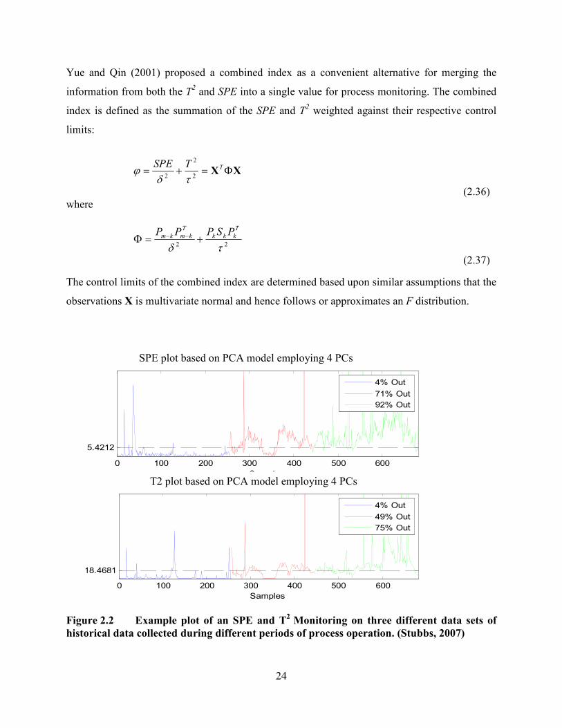
Figure 2.2 provides an example illustration of the application of the T2 and Q statistics

monitoring. The application is an excerpt taken from results documented by the author in a

previous MSc. dissertation (Stubbs, 2007).

24

Yue and Qin (2001) proposed a combined index as a convenient alternative for merging the

information from both the T2 and SPE into a single value for process monitoring. The combined

index is defined as the summation of the SPE and T2 weighted against their respective control

limits:

XX Φ=+= TTSPE2

2

2 τδϕ

(2.36)

where

22 τδ

T

kkk

T

kmkm PSPPP+=Φ −−

(2.37)

The control limits of the combined index are determined based upon similar assumptions that the

observations X is multivariate normal and hence follows or approximates an F distribution.

Figure 2.2 Example plot of an SPE and T2

Monitoring on three different data sets of

historical data collected during different periods of process operation. (Stubbs, 2007)

0 100 200 300 400 500 600

18.4681

T2 plot using 4 PCsbatch(es): R6G8

Score Residue

Samples

0 100 200 300 400 500 600

5.4212

Partial Model SPE using 4 PCs, experimental batch(es): R6G8

Residuals

Samples

4% Out

49% Out

75% Out

4% Out

71% Out

92% Out

SPE plot based on PCA model employing 4 PCs

T2 plot based on PCA model employing 4 PCs

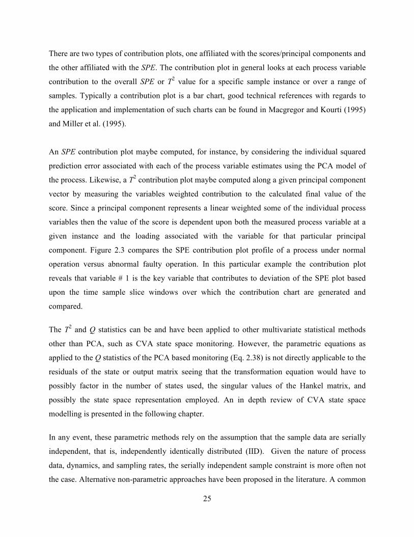
25

There are two types of contribution plots, one affiliated with the scores/principal components and

the other affiliated with the SPE. The contribution plot in general looks at each process variable

contribution to the overall SPE or T2 value for a specific sample instance or over a range of

samples. Typically a contribution plot is a bar chart, good technical references with regards to

the application and implementation of such charts can be found in Macgregor and Kourti (1995)

and Miller et al. (1995).

An SPE contribution plot maybe computed, for instance, by considering the individual squared

prediction error associated with each of the process variable estimates using the PCA model of

the process. Likewise, a T2 contribution plot maybe computed along a given principal component

vector by measuring the variables weighted contribution to the calculated final value of the

score. Since a principal component represents a linear weighted some of the individual process

variables then the value of the score is dependent upon both the measured process variable at a

given instance and the loading associated with the variable for that particular principal

component. Figure 2.3 compares the SPE contribution plot profile of a process under normal

operation versus abnormal faulty operation. In this particular example the contribution plot

reveals that variable # 1 is the key variable that contributes to deviation of the SPE plot based

upon the time sample slice windows over which the contribution chart are generated and

compared.

The T2 and Q statistics can be and have been applied to other multivariate statistical methods

other than PCA, such as CVA state space monitoring. However, the parametric equations as

applied to the Q statistics of the PCA based monitoring (Eq. 2.38) is not directly applicable to the

residuals of the state or output matrix seeing that the transformation equation would have to

possibly factor in the number of states used, the singular values of the Hankel matrix, and

possibly the state space representation employed. An in depth review of CVA state space

modelling is presented in the following chapter.

In any event, these parametric methods rely on the assumption that the sample data are serially

independent, that is, independently identically distributed (IID). Given the nature of process

data, dynamics, and sampling rates, the serially independent sample constraint is more often not

the case. Alternative non-parametric approaches have been proposed in the literature. A common

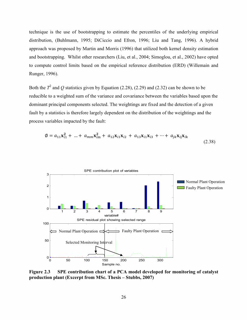
26

technique is the use of bootstrapping to estimate the percentiles of the underlying empirical

distribution, (Buhlmann, 1995; DiCiccio and Efron, 1996; Liu and Tang, 1996). A hybrid

approach was proposed by Martin and Morris (1996) that utilized both kernel density estimation

and bootstrapping. Whilst other researchers (Liu, et al., 2004; Simoglou, et al., 2002) have opted

to compute control limits based on the empirical reference distribution (ERD) (Willemain and

Runger, 1996).

Both the T2 and Q statistics given by Equation (2.28), (2.29) and (2.32) can be shown to be

reducible to a weighted sum of the variance and covariance between the variables based upon the

dominant principal components selected. The weightings are fixed and the detection of a given

fault by a statistics is therefore largely dependent on the distribution of the weightings and the

process variables impacted by the fault:

∅ = [11p/1" +)…+)[@@p/~" +)[1?p/1p/?) +)[1�p/1p/�) +⋯+)[g^p/�p/�) (2.38)

Figure 2.3 SPE contribution chart of a PCA model developed for monitoring of catalyst

production plant (Excerpt from MSc. Thesis – Stubbs, 2007)

1 2 3 4 5 6 7 8 90

1

2

3SPE contribution plot of variables

Scaled variable contribution

variable#

0 50 100 150 200 250 3000

50

100SPE residual plot showing selected range

Square Prediction Error, SPE

Sample no.

Faulty Plant Operation

Normal Plant Operation

Normal Plant Operation Faulty Plant Operation

Selected Monitoring Interval

27

2.5 Multiblock and Multiway PCA/PLS methods and Interval PLS (IPLS) Multi-block PLS (MBPLS) and multi-way PCA are yet another variant to PCA and PLS intended

at adapting the methods to better suit batch processes with time dependencies and those

processes involving a very large number of variables.

2.5.1 Multiblock Partial Least Squares

In MBPLS approach, large sets of process variables (X) are divided in to smaller meaningful

sub-blocks, for instance each block may be associated with a specific section of the plant or a

specific process unit. From this multivariate control charts for the important subsection of the

plant and the entire plant can be constructed.

In the Multiblock PLS approach the sub-blocks are weighted in such a way that they are most

predictive of Y thus the monitoring space is determined by the combined model and not by

separate models for each block. Details of the theory and algorithm for the implementation of

MBPLS are documented in the works of Wangen and Kowalski (1989) and more recently by

Westerthuis and Coenegracht (1997). These two algorithms are different in the sense that the

early publication proposed deflates the X and Y blocks using the block scores while the more

recent publications have endorsed deflation by way of the super-scores. It turns out that the latter

approach leads to superior predictive performance equivalent to that which would have been

obtained using the unfolded matrix and application of the traditional PLS method (Lopes, et al.

2002). In an application of MBLS to an industrial pharmaceutical process, Lopes et al. (2002)

modelled the production of an active pharmaceutical ingredient by fermentation. The

observations gathered over thirty batch runs where separated into four data blocks of

manipulated and quality variables for incolium production stage and the API production

fermentation stage.

28

2.5.2 Multiway PLS and PCA

Multiway partial least squares is an extension of PLS to deal with data in three dimension arrays.

By three dimensions we refer to variables sampled over a fix time duration collected across

several batches (repeat runs of the same process). The multiway technique of transforming a

three dimensional data set into a two dimensional representation was first introduced and applied

to PCA and PLS by Wold et al. (1987), and was followed up by several other key publications

(Nomikos and MacGregor, 1995; Kosanovich, et al., 1994). Since then there have been many

publications on the applications of MPCA, MPLS, and their variants such as batch dynamic PCA

and PLS (Chen and Liu, 2002; Hu and Yuan, 2008). The MPLS is essentially the equivalent of

PLS applied to the unfolded three dimension data set X (I × J × K) where I is the number of

batches J is the number of variables and K represents the number of measurement sample for the

duration of the batch run. As shown in Figures 2.4 to 2.6 the data can be unfolded in one of three

different modes: i) Time ii) Batch and iii) Variable.

Figure 2.4 Time-mode Unfolding

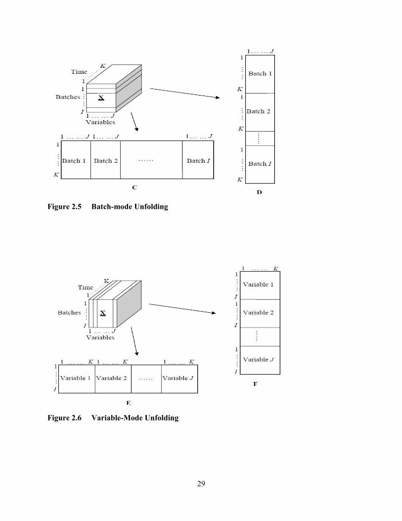
29

Figure 2.5 Batch-mode Unfolding

Figure 2.6 Variable-Mode Unfolding

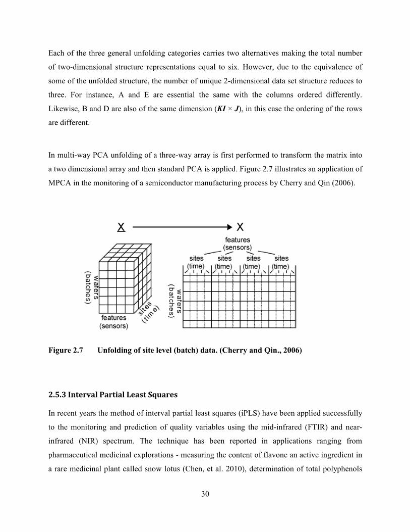
30

Each of the three general unfolding categories carries two alternatives making the total number

of two-dimensional structure representations equal to six. However, due to the equivalence of

some of the unfolded structure, the number of unique 2-dimensional data set structure reduces to

three. For instance, A and E are essential the same with the columns ordered differently.

Likewise, B and D are also of the same dimension (KI × J), in this case the ordering of the rows

are different.

In multi-way PCA unfolding of a three-way array is first performed to transform the matrix into

a two dimensional array and then standard PCA is applied. Figure 2.7 illustrates an application of

MPCA in the monitoring of a semiconductor manufacturing process by Cherry and Qin (2006).

Figure 2.7 Unfolding of site level (batch) data. (Cherry and Qin., 2006)

2.5.3 Interval Partial Least Squares

In recent years the method of interval partial least squares (iPLS) have been applied successfully

to the monitoring and prediction of quality variables using the mid-infrared (FTIR) and near-

infrared (NIR) spectrum. The technique has been reported in applications ranging from

pharmaceutical medicinal explorations - measuring the content of flavone an active ingredient in

a rare medicinal plant called snow lotus (Chen, et al. 2010), determination of total polyphenols

31

content in green tea (Chen, et al. 2008), and for simultaneous active substance detection in

pharmaceutical formulations (Silva, et al. 2009), to the detection of quality parameters in

biodiesel/diesel blends (Ferrao, et al. 2011) and the detection of contaminants in lubricating oil

(Borin and Poppi, 2005). The principle of this method involves splitting a spectrum or batch

duration into several equidistance sub-intervals or regions and then developing PLS algorithm

for each sub-interval using a select number of latent variables. This iPLS approach will be

employed and applied to the batch-wise unfolded data set to produce Multiway iPLS (MiPLS)

monitoring and predictive models in Chapter 6.

2.6 Dynamic PCA and PLS

The PCA model is limited to capturing only the static underlying correlation and cross-

covariance structure between the process variables. This is a direct result of the scores or latent

variables being based only on the current time samples of all the process variables as shown in

Eq. (2.6). In a dynamic system the current state or values of the process outputs (variables) are

also dependent upon the past values. Therefore, a representative model would be required not

only to capture the linear relation between the variables at the current time t but also the serial

correlation (autocorrelation), the relationship between X(t) and previous instances - X(t-1), X(t –

2), and so forth. PCA can be extended to dynamic system by carrying out a matrix expansion of

the original data matrix with time-shifted duplicated vectors. By appropriate selection of the

number of lags l to be included - X(t – l), both the static and dynamic relationship between the

variables can be accounted for.

Xd = [X(k) X(k-1) ……X(k-l)]

(2.39)

One of the earlier publications describing the extension of PCA to dynamic multivariate

statistical monitoring was by Ku, et al. (1995) in which the theoretical basis and justification of

the approach was presented. More recently Liu, et al. (2004) look at the application of DPCA to

enhance chunk monitoring of an industrialized fluidized-bed reactor and explored several

methods of selecting the number of lags l to be used. The additional task of identifying the

number of lag terms to be used in the dynamic model is a major drawback associated with the

dynamic model extension of PCA and will also apply in the case of dynamic partial least squares

32

(DPLS) and CVA. The selection process becomes an even more challenging task when the

dynamic expansion is to be carried out on a variable-dependent basis. There is also the risk of the

dynamic matrix given by Eq. (2.40) being ill-conditioned due to strong serial correlation in the

measurement data.

As it relates to DPLS there are few different approaches to incorporating the time-shifted data

variables. This can be applied only on the X block as carry out by Ricker (1988), both orthogonal

decomposition and PLS decomposition was applied to the Xd matrix to improve the conditioning

of the matrix and subsequent the estimation of regression parameters. Alternatively dynamic

expansion of both the X and Y block can be carried out as done by Qin and McAvoy (1993) to

reflect an autoregressive moving average (ARMA) time series mathematical model. In a later

publication dynamic PLS was combined with a neural network approach to develop a non-linear

finite impulse response FIR model (Qin and McAvoy, 1996). The ARMA time series model

includes past values of the response (output) variables as part of the dynamic expansion of the X

block unlike the FIR model:

�� = A�� , �� − 1 ,⋯ �� − �� , �� − 1 , �� − 2 …,)))�� − �� C (2.40)

where lx is the number of lags on the input and ly is the number of lags on the outputs.

Lakshminarayanan, et al. (1997) chose to build a dynamic regression model to define the inner

relation between the time-shifted scores of the X and Y blocks without expansion of the original

variable block with time-shifted process variables.

The major drawback of these dynamic projection methods is the increased numerical

computation involving a much larger data set with the time-shifted variable duplications added

on. A limited number of the published applications have actually explored defining variable

specific lags as different process variables will have different dynamics. Simoglou, et al. (1999a)

applied such an approach in the development of a DPLS and CVA statistical model of a binary

distillation column.

33

2.7 Summary

Multivariate statistical process controls is an extension of univariate SPC that has proven to be a

more effective statistical approach to process monitoring because it accounts for both the

variance and covariance structure in a data set. PCA and PLS are the two corner stone projection

methods of MSPC from which several offshoots have emerged. These offshoots have emerged

out of necessity to address issues relating to improve modelling and monitoring of dynamic,

nonlinear processes, and batch processes.

In the case of dynamic processes – DPCA and DPLS have been proposed as extensions to to

PCA and PLS respectively. For batch processes Multi-way and Multi-block PLS and PCA have

evolved to more effectively capture the correlation structure across the batches and sub block of

process variables of different types.

Finally, the literature review touched on the two most common monitoring statistics –

Hotelling’s T2 square and Q statistics. The review presented on some of the equations that been

proposed for computing the control limit of these statistics

34

Chapter 3 : Review of Subspace, Non-linear and

Hybrid Modelling Techniques

3.1 Introduction

Subspace system identification is a very popular system identification method that has been

around since the early eighties. The popularity is owed to the advantages that the modelling

technique and algorithm offers over other methods. In particularly, they are non-iterative, and

robust as they employ primarily numerically stable mathematical methods of linear algebra.

They are well suited to modelling multiple-input multiple output systems providing reliable state

space model alternatives to polynomial based models and models based on instrumental variable

method (Borjas and Garcia, 2010).

State Space modelling is a class of subspace modelling that seeks to model, monitor and/or

control the process by successive approximation of the memory or states of the process.

Approximation of the states of the process may be carried out in a number of different ways:

PLS, numerical algorithms for state space subspace system identification (N4SID); balanced

realisation (BR) and canonical correlation regression CCR. Comparisons with CVA against these

alternatives have been carried out (Juricek, et al. 2005; Negiz and Cinar, 1997b; Simoglou, et al.,

1999a) and they have all concluded that CVA outperforms the other methods in terms of model

stability and parsimony. Several methods used for identifying the dimension of the subspace

35

model in terms of the number of lags, states and other modelling parameters have been applied in

the literature and will be reviewed in this chapter.

One can usually assume that the process behaves fairly linear within the region of its operating

conditions, however when this is not the case application of linear PCA and PLS methods may

generate erroneous results and lead to misleading interpretation (Dong and McAvoy, 1996b).

Several nonlinear extensions to PCA and PLS proposed in the literature will be particularly

applicable to processes whose variability are characterized by significant nonlinearity. Other

approaches to quantifying and effectively model nonlinear process dynamics have applied hybrid

models combining mechanistic and data driven statistical models (Lee, et al. 2005; Oliveira

2004; Peres, et al. 2001; Psichogios and Ungar, 1992).

This chapter will review three subspace algorithms. Section 3.2 will review an algorithm

proposed by Larimore (Larimore, 1983; Larimore, 1990) which employs the mathematics of

principal angles and directions to identify a canonical correlation structure upon which the

subspace model predictive capabilities are based. In section 3.3 two other algorithms are

explored in less detail – MOESP proposed by Verhaegen (1994) and stands for Multiple Output

Error State Space, and N4SID by Van Overschee and De Moor (1994). N4SID stands for

‘numerical algorithms for subspace state space system identification’. Section 3.4 provides an

overview of several model selection criterion and procedures that have been applied in the

literature. Section 3.5 discusses several nonlinear extensions to linear projections and dynamic

subspace methods covered in this and the previous chapter. Section 3.6 revisits several hybrid

models that have been applied in the literature for prediction and process monitoring

applications. Section 3.7 provides a summary overview of the modelling approaches reviewed in

the chapter.

3.2 Canonical Variate Analysis and State Space Approach

Canonical Correlation Analysis (CCA) was first introduced by Hotelling sometime between

1933 and 1936 based on the accounts of Negiz and Cinar (1997b). It was later applied to linear

dynamic system modelling and Markovian state space system identification by Akaike, see

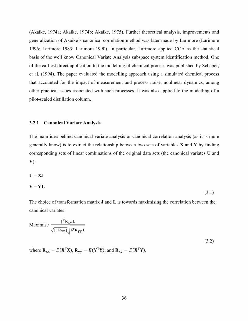
36

(Akaike, 1974a; Akaike, 1974b; Akaike, 1975). Further theoretical analysis, improvements and

generalization of Akaike’s canonical correlation method was later made by Larimore (Larimore

1996; Larimore 1983; Larimore 1990). In particular, Larimore applied CCA as the statistical

basis of the well know Canonical Variate Analysis subspace system identification method. One

of the earliest direct application to the modelling of chemical process was published by Schaper,

et al. (1994). The paper evaluated the modelling approach using a simulated chemical process

that accounted for the impact of measurement and process noise, nonlinear dynamics, among

other practical issues associated with such processes. It was also applied to the modelling of a

pilot-scaled distillation column.

3.2.1 Canonical Variate Analysis

The main idea behind canonical variate analysis or canonical correlation analysis (as it is more

generally know) is to extract the relationship between two sets of variables X and Y by finding

corresponding sets of linear combinations of the original data sets (the canonical variates U and

V):

U = XJ

V = YL

(3.1)

The choice of transformation matrix J and L is towards maximising the correlation between the

canonical variates:

Maximise ��i��)��i��)�4��i��)�

(3.2)

where i�� = =�� , i�� = =O�O , and i�� = =��O .

37

The objective specified by Eq. (3.2) is equivalent to solving the following constrained

optimization problem:

∅ = ��i�� + ��#� − ��i�� + ��f#� − ��i��h

(3.3)

where Ix and Iy are identity matrices of appropriate dimensions and λx and λy are the Lagrange

constants. The solution to Eq (3.3) commences with differentiating the function with respect to J

and L and solving the resulting pair of simultaneous equation below:

]∅ ]�3 = ��i�� − "��i�� = 0

(3.4)

]∅ ]�3 = ��i�� − ��i�� = 0

(3.5)

The solution is given by:

��fi��1/?i��i��1/?h = ��

(3.6)

� = i��1/?��; � = i��1/?��

(3.7)

The main diagonal of the S matrix contains the correlation coefficients. The combined operation

of Eq. (3.6) and Eq. (3.7) is referred to as the generalized singular value decomposition (GSVD)

of Rxy.

CVA is conceptually similar to DPLS, in that both method seek to extract a subspace

representation of the correlation between two blocks of data set. A comparison of Balanced,

PLS, CV state space realization by Negiz and Cinar (1997b) revealed that the three approaches

were all capable of identifying a minimal state order model but concluded that the CV state space

realization offered a much more robust tool for system identification in state space than PLS and

the balanced realization methods. The main advantage offered by CVA realization is that it

generates states that are orthogonal at zero lag and requires a one-step SVD algorithm to arrive at

the states. The classical PLS algorithm, however, requires an additional SVD step in order for the

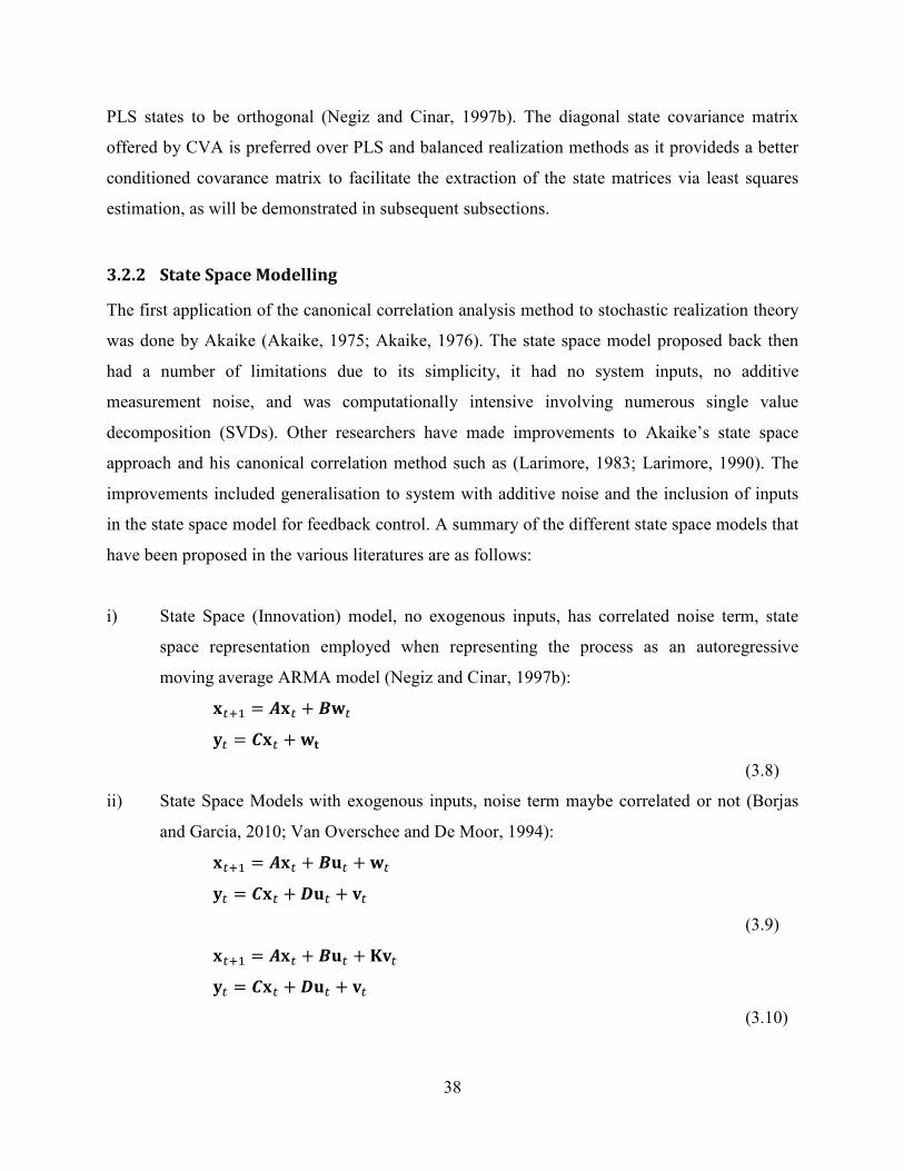
38

PLS states to be orthogonal (Negiz and Cinar, 1997b). The diagonal state covariance matrix

offered by CVA is preferred over PLS and balanced realization methods as it provideds a better

conditioned covarance matrix to facilitate the extraction of the state matrices via least squares

estimation, as will be demonstrated in subsequent subsections.

3.2.2 State Space Modelling

The first application of the canonical correlation analysis method to stochastic realization theory

was done by Akaike (Akaike, 1975; Akaike, 1976). The state space model proposed back then

had a number of limitations due to its simplicity, it had no system inputs, no additive

measurement noise, and was computationally intensive involving numerous single value

decomposition (SVDs). Other researchers have made improvements to Akaike’s state space

approach and his canonical correlation method such as (Larimore, 1983; Larimore, 1990). The

improvements included generalisation to system with additive noise and the inclusion of inputs

in the state space model for feedback control. A summary of the different state space models that

have been proposed in the various literatures are as follows:

i) State Space (Innovation) model, no exogenous inputs, has correlated noise term, state

space representation employed when representing the process as an autoregressive

moving average ARMA model (Negiz and Cinar, 1997b):

p��1 = !p� + j�� = �p� +��

(3.8)

ii) State Space Models with exogenous inputs, noise term maybe correlated or not (Borjas

and Garcia, 2010; Van Overschee and De Moor, 1994):

p��1 = !p� + j�� +�� = �p� + �� + �

(3.9)

p��1 = !p� + j�� + �� = �p� + �� + �

(3.10)

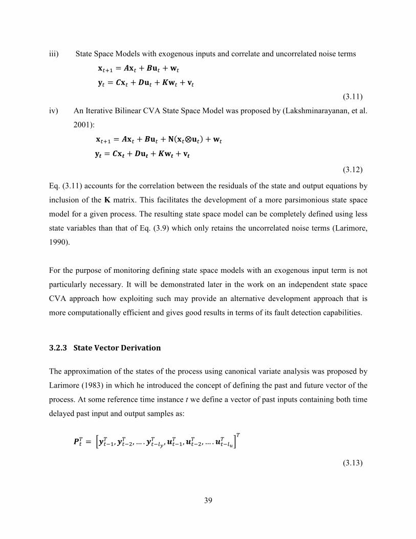
39

iii) State Space Models with exogenous inputs and correlate and uncorrelated noise terms

p��1 = !p� + j�� +��

�� = �p� + �� +�� + �

(3.11)

iv) An Iterative Bilinear CVA State Space Model was proposed by (Lakshminarayanan, et al.

2001):

p��1 = !p� + j�� + �p�⨂�� + ��

�2 = �p2 + ��2 +��2 + 2

(3.12)

Eq. (3.11) accounts for the correlation between the residuals of the state and output equations by

inclusion of the K matrix. This facilitates the development of a more parsimonious state space

model for a given process. The resulting state space model can be completely defined using less

state variables than that of Eq. (3.9) which only retains the uncorrelated noise terms (Larimore,

1990).

For the purpose of monitoring defining state space models with an exogenous input term is not

particularly necessary. It will be demonstrated later in the work on an independent state space

CVA approach how exploiting such may provide an alternative development approach that is

more computationally efficient and gives good results in terms of its fault detection capabilities.

3.2.3 State Vector Derivation

The approximation of the states of the process using canonical variate analysis was proposed by

Larimore (1983) in which he introduced the concept of defining the past and future vector of the

process. At some reference time instance t we define a vector of past inputs containing both time

delayed past input and output samples as:

H�� =) ¡¢��1� , ¢��?� , … . ¢��;£� , _��1� , _��?� , … . _��;¤� ¥�

(3.13)

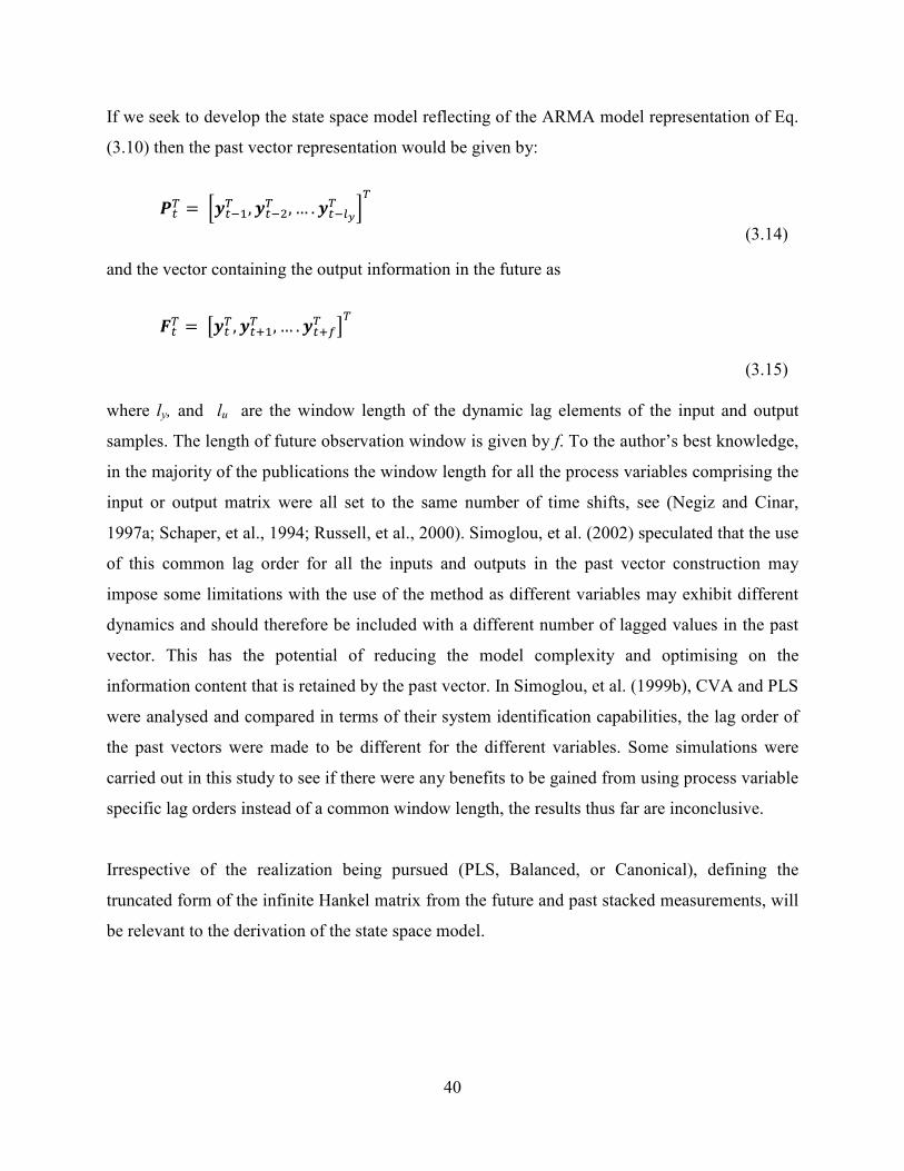
40

If we seek to develop the state space model reflecting of the ARMA model representation of Eq.

(3.10) then the past vector representation would be given by:

H�� =) ¡¢��1� , ¢��?� , … . ¢��;£� ¥�

(3.14)

and the vector containing the output information in the future as

`�� =) A¢�� , ¢��1� , … . ¢��¦� C�

(3.15)

where ly, and lu are the window length of the dynamic lag elements of the input and output

samples. The length of future observation window is given by f. To the author’s best knowledge,

in the majority of the publications the window length for all the process variables comprising the

input or output matrix were all set to the same number of time shifts, see (Negiz and Cinar,

1997a; Schaper, et al., 1994; Russell, et al., 2000). Simoglou, et al. (2002) speculated that the use

of this common lag order for all the inputs and outputs in the past vector construction may

impose some limitations with the use of the method as different variables may exhibit different

dynamics and should therefore be included with a different number of lagged values in the past

vector. This has the potential of reducing the model complexity and optimising on the

information content that is retained by the past vector. In Simoglou, et al. (1999b), CVA and PLS

were analysed and compared in terms of their system identification capabilities, the lag order of

the past vectors were made to be different for the different variables. Some simulations were

carried out in this study to see if there were any benefits to be gained from using process variable

specific lag orders instead of a common window length, the results thus far are inconclusive.

Irrespective of the realization being pursued (PLS, Balanced, or Canonical), defining the

truncated form of the infinite Hankel matrix from the future and past stacked measurements, will

be relevant to the derivation of the state space model.

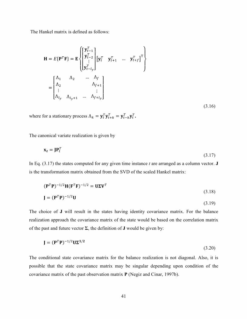
41

The Hankel matrix is defined as follows:

§ = =¨M�R© = Nª«¬«®° ��1��?�⋮��;£� ²³³

³ A�� 1� … ��¦� C�µ«¶«·

=®° Λ1 Λ? … Λ¦Λ? Λ¦�1⋮Λ;£ Λ;£�1 ⋮… Λ¦�;£²³³

³

(3.16)

where for a stationary process Λ^ = ��^� = ��^� ��.

The canonical variate realization is given by

p2 = �M��

(3.17)

In Eq. (3.17) the states computed for any given time instance t are arranged as a column vector. J

is the transformation matrix obtained from the SVD of the scaled Hankel matrix:

M�M �1/?§R�R �1/? = P��

(3.18)

� = M�M �1/?P

(3.19)

The choice of J will result in the states having identity covariance matrix. For the balance

realization approach the covariance matrix of the state would be based on the correlation matrix

of the past and future vector Σ, the definition of J would be given by:

� = M�M �1/?P��/"

(3.20)

The conditional state covariance matrix for the balance realization is not diagonal. Also, it is

possible that the state covariance matrix may be singular depending upon condition of the

covariance matrix of the past observation matrix P (Negiz and Cinar, 1997b).

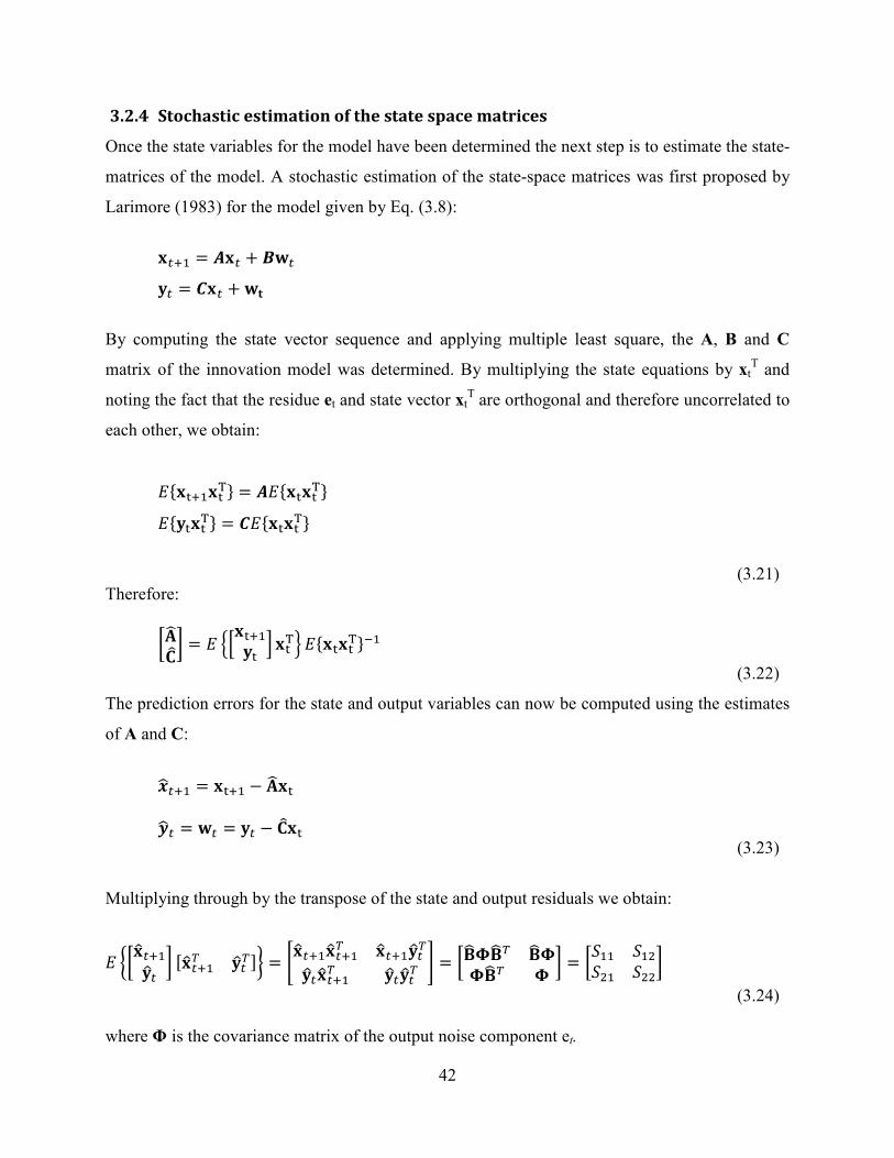
42

3.2.4 Stochastic estimation of the state space matrices

Once the state variables for the model have been determined the next step is to estimate the state-

matrices of the model. A stochastic estimation of the state-space matrices was first proposed by

Larimore (1983) for the model given by Eq. (3.8):

p��1 = !p� + j�� = �p� +��

By computing the state vector sequence and applying multiple least square, the A, B and C

matrix of the innovation model was determined. By multiplying the state equations by xtT and

noting the fact that the residue et and state vector xtT are orthogonal and therefore uncorrelated to

each other, we obtain:

=¨p¹�1p¹�© = !=¨p¹p¹�© =¨�¹p¹�© = �=¨p¹p¹�©

(3.21)

Therefore:

º�w»¼½ = = ¾¡p¹�1�¹ ¥ p¹�¿ =¨p¹p¹�©�1

(3.22)

The prediction errors for the state and output variables can now be computed using the estimates

of A and C:

ÀÁ��1 = p¹�1 − �wp¹

¢Á� = �� = �� − »¼p¹ (3.23)

Multiplying through by the transpose of the state and output residuals we obtain:

= ÂºpÃ��1�Ã� ½ GpÃ��1� �Ã��JÄ = DpÃ��1pÃ��1� pÃ��1�Ã��Ã�pÃ��1� �Ã��Ã�� E = ºÅwÆÅw� ÅwÆÆÅw� Æ ½ = º�11 �1?�?1 �??½ (3.24)

where Φ is the covariance matrix of the output noise component et.

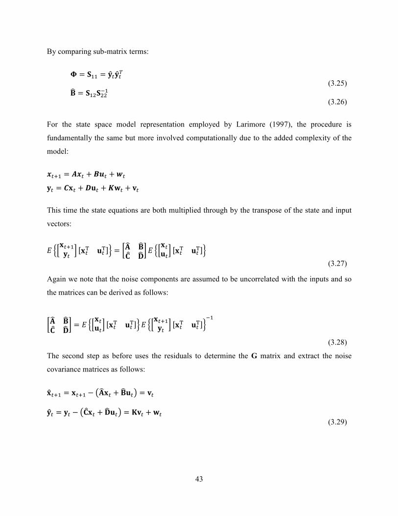
43

By comparing sub-matrix terms:

Æ = �11 = �Ã��Ã��

(3.25)

Åw = �1?�??�1 (3.26)

For the state space model representation employed by Larimore (1997), the procedure is

fundamentally the same but more involved computationally due to the added complexity of the

model:

À��1 = !À� + j_� +V� �� = �p� + �� +�� + �

This time the state equations are both multiplied through by the transpose of the state and input

vectors:

= ¾¡p��1�� ¥ Gp�� J¿ = º�w Åw»¼ Çw½= ¾¡p��¥ Gp�� J¿ (3.27)

Again we note that the noise components are assumed to be uncorrelated with the inputs and so

the matrices can be derived as follows:

º�w Åw»¼ Çw½ = = ¾¡p��¥ Gp�� J¿ = ¾¡p��1�� ¥ Gp�� J¿�1

(3.28)

The second step as before uses the residuals to determine the G matrix and extract the noise

covariance matrices as follows:

pÃ��1 = p��1 − f�wp� + Åw��h = � �Ã� = �� − f»¼p� + Çw��h = �� +�� (3.29)

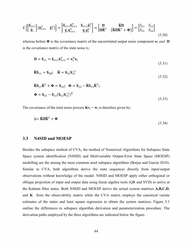
44

= ÂºpÃ��1�Ã� ½ GpÃ��1� �Ã��JÄ = DpÃ��1pÃ��1� pÃ��1�Ã��Ã�pÃ��1� �Ã��Ã�� E = º È �wÈÈ�w� f�wÈ�w� +Æh½ = º�11 �1?�?1 �??½ (3.30)

whereas before Φ is the covariance matrix of the uncorrelated output noise component wt and Π

is the covariance matrix of the state noise vt:

È = �11 = pÃ��1pÃ��1� = �� (3.31)

�w�11 = ��"; �w = �1?�11�1

(3.32)

�w�11�w� +Æ = �??; Æ = �?? − �w�11�w�;

Æ = �?? − �1?�1?�11�1 �

(3.33)

The covariance of the total noise process Kvt + wt is therefore given by:

∆= �wÈ�w� +Æ

(3.34)

3.3 N4SID and MOESP

Besides the subspace method of CVA, the method of Numerical Algorithms for Subspace State

Space system identification (N4SID) and Multivariable Output-Error State Space (MOESP)

modelling are the among the most common used subspace algorithms (Borjas and Garcia 2010).

Similar to CVA, both algorithms derive the state sequences directly from input/output

observations without knowledge of the model. N4SID and MOESP apply either orthogonal or

oblique projection of input and output data using linear algebra tools (QR and SVD) to arrive at

the Kalman filter states. Both N4SID and MOESP derive the actual system matrices A,B,C,D,

and K from the observability matrix while the CVA matrix employs the canonical variate

estimates of the states and least square regression to obtain the system matrices. Figure 3.1

outline the differences in subspace algorithm derivation and parameterization procedure. The

derivation paths employed by the three algorithms are indicated below the figure.

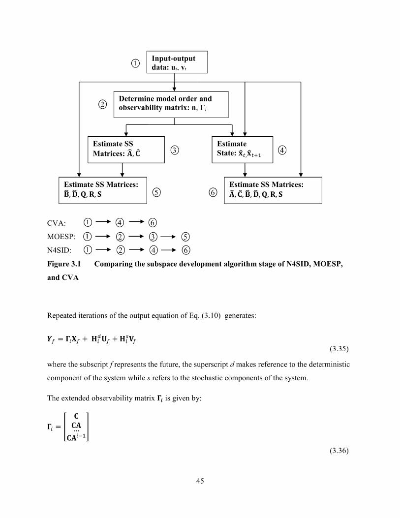
45

CVA:

MOESP:

N4SID:

Figure 3.1 Comparing the subspace development algorithm stage of N4SID, MOESP,

and CVA

Repeated iterations of the output equation of Eq. (3.10) generates:

|¦ = Ê/�¦ +)§/<P¦ + §/Ë�¦

(3.35)

where the subscript f represents the future, the superscript d makes reference to the deterministic

component of the system while s refers to the stochastic components of the system.

The extended observability matrix Ê/ is given by:

Ê/ = Ì »»�…»�/�1Í (3.36)

Input-output

data: ut, yt

Determine model order and

observability matrix: n, Γi

Estimate

State: pÃ�,pÃ��1

Estimate SS

Matrices: �w, »¼

Estimate SS Matrices: Åw,Çw , Q, i, �

Estimate SS Matrices: �w, »¼, Åw, Çw , Q, i, �

1

2

3 4

5 6

1 4 6

1 2 3 5

1 2 4 6

46

§/< is a lower block triangular Toeplitz matrix given by:

)§/< = ®° Ç 0 0 … 0»Å Ç 0 … 0»�Å…»�Î�?Å

»Å…»�Î��ÅÇ……

……»Å0…D²³³³

(3.37)

While the covariance matrix §/Ë is given by:

§/< =®¯° v/ v/�1 v/�? … v1v/�1 v/ v/�1 … v?v/�?…v?/�1

v/�1…v?/�?v/……

……v/�1v�…v/ ²³³³ = Ê/Ð/Ë and v/ = Ñ»�Î�1Ò ))))))Ó > 0v/ )))))))))))))))Ó = 0A»�Î�1ÒC� )Ó < 0

(3.38)

The G matrix is a cross-covariance matrix defined as:

Ö = =×p^��Ø. (3.39)

The past and future input and output block-Hankel matrices are defined as:

PB =®¯° uÚ u1 ))))u? ))… ug�1u1 u? u� ))… ug⋮u/�?u/�1

⋮…u/⋮))…)))))))u/�1

………⋮u/�g��u/�g�?²³

³³

(3.40)

where Û^ ∈ ℝ@ is the input vector observation at the kth time instance. The output Yp, Yf, and

noise Vp, Vf Block-Hankel are all similarly constructed.

P¦ =®¯° u/ u/�1 ))))u? ))… u/�g�1u/�1 u/�? u/�� … u/�g⋮u?/�?u?/�1

⋮…u?/ ) ⋮…))u?/�1………

⋮u?/�g��u?/�g�?²³³³

47

The MOESP solves the subspace problem by first deriving an approximation of the extended

observability matrix Ê/. This is achieved by eliminating the last two terms in the right side of Eq.

(3.35) and is carried out in two steps:

i) An orthogonal projection of Eq. (3.35) is performed into the row space of Þ¦ß and

yields:

|¦/Þ¦ß = Ê/�¦/Þ¦ß +)§/<P¦/Þ¦ß + §/Ë�¦/Þ¦ß

(3.41)

Applying one of the properties of orthogonal projection (P¦/Þ¦ß = 0), Eq. (3.41) can

be simplified to:

|¦/Þ¦ß = Ê/�¦/Þ¦ß +)§/Ë�¦/Þ¦ß

(3.42)

ii) To eliminate the noises term in Eq. (3.42), the equation is multiplied by an

instrumental variable à = fPB�OBh� and this yields:

|¦/Þ¦ßá = Ê/�¦/Þ¦ßá +)§/Ë�¦/Þ¦ßá

(3.43)

Since it is assumed that the noise is uncorrelated with the input and output past data then that

would mean �¦/Þ¦ßá)) = â and therefore Eq. (3.43) is further simplified to:

|¦/Þ¦ßá = Ê/�¦/Þ¦ßá) (3.44)

From Eq. (3.44) the estimates of the Kalman filter state is given by �w¦ = �¦/Þ¦ßá and the

column space of Ê/ can be calculated from the SVD of |¦/Þ¦ßá.

48

N4SID arrives at an alternative subspace model solution to the problem by means of an

approximation of the past and future Kalman filter state sequence. First an oblique projection of

Eq (3.35) is carried out along the row space of Uf onto the row space of Z:

|¦/ãäá = Ê/�¦/ãäá +)§/<P¦/ãäá + §/Ë�¦/ãäá

(3.45)

The last two terms of the Eq. (3.45) are zero by the property of oblique projection and based

upon the assumption that the noise is uncorrelated with input and output past data. Based upon

theorem in Overschee and Moor (1996), Eq. (3.45) can be written as:

å/ = Ê/�w/ (3.46)

where �w/ = �¦/ãäá and å/ = |¦/ãäá.

It was shown in Overschee and Moor (1996) that the column space and of Ê/ can be calculated

from the SVD of å/: Ê/ = æ1�11/?

(3.47)

With Ê/ and å/ known the state sequence �w/ can be computed easily by applying Eq. (3.46) and

the next state can also be calculated as:

�w/�1 = Ê/�1�1å/�1

(3.48)

where å/�1 = |¦�/ÞäçáB� and Ê/�1 denotes the matrix Ê/ without the last l rows.

Several other subspace algorithms have been proposed in the literature for identification of

combine deterministic-stochastic systems. The subspace algorithm proposed by Viberg, et al.

(1993) in an instrumental variable framework was shown to be an equivalent to N4SID

algorithms in terms of how the model order and observability matrix Ê/ are determined

(Overschee and Moor, 1995). More recently Borjas and Garcia (2010) proposed an hybrid

49

algorithm merging the N4SID method with the MOESP approach. The algorithm employs the

MOESP method to extract the obervability matrix and then use the N4SID method to calculate

the matrices A,B,C,D through least squares regression.

An interpretation of Larimore’s CVA subspace method in an effort to summarize the similarities

and difference that exist between the method versus MOESP and N4SID subspace identification

methods is presented in Overschee and Moor (1995). Reference was made to the analysis and

description of the CVA method Larimore provided (Larimore, 1990). In order to compare the

method with the N4SID and MOESP approach it was necessary to establish the parallels between

the notations employed by Larimore and those used previously in describing the N4SID and

MOESP method, the definition are as follows:

i) the past inputs and outputs matrix

b ≝ éÞB|Bê

( 3.49)

ii) the future outputs

ë ≝ |¦

( 3.50)

iii) and the future inputs (not included in the analysis in Section 3.2)

_ ≝ Þ¦

( 3.51)

In relation to the analysis presented in Section 3.2 the notations p and f are equivalent to P and F

respectively.

The primary goal of a system identification model can be categorized as given in Overschee and

Moor (1995):

i) Optimal prediction. To arrive at a model that will sufficiently accurately predict the

behaviour of the process variables. For the linear subspace system identification case

this may be formulated mathematically as finding the optimal linear combination of

50

the past input-outputs b and future inputs _ to predict the future state of the outputs ë:

ì��b,�_ íë − �B �î �b_�íï"

( 3.52)

where �B ∈ ℝ��)×)ì�� e and �î ∈ ℝ��)×)ì�

The optimal combination of the past input/outputs p to predict the future f can be

geometrically interpreted as the oblique projection of the row space of f along the row

space of p:

ñ ≝ �Bb

( 3.53)

ii) Complexity reduction. A second goal is that for a given model accuracy, the complexity

of the model should be limited to its minimal dimension. This second requirement can be

mathematically formulated as:

) ì��òZó1ñ − ò ó?Zï"

(3.54)

where ò ∈ ℝ;/)p)g, n1 ∈ ℝ;/)p);/)and n? ∈ ℝg)p)g). The choice of the weighting matrices

W1 and W2 determines the information retained by the reduced subspace representation ò

of the model ñ. The choice of weightings, as shown in Table 3.1, is also the basis of

distinction between the different subspace methods covered in this literature review. The

solution to Eq. (3.54) for the optimal reduction is given by:

ò = ó1��Þ1ô1�1�ó?��

( 3.55)

where the following SVD gives:

ó1ñó? = Þ1 Þ? �ô1 00 0� õ�1��?�ö

( 3.56)

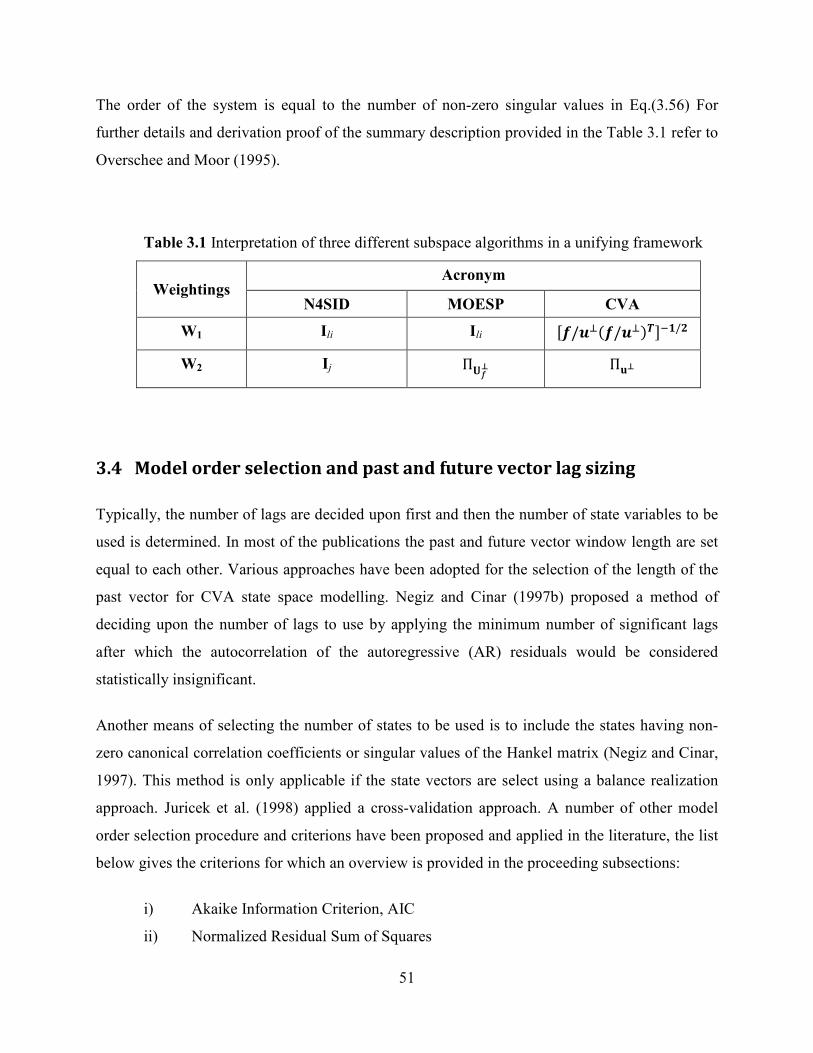
51

The order of the system is equal to the number of non-zero singular values in Eq.(3.56) For

further details and derivation proof of the summary description provided in the Table 3.1 refer to

Overschee and Moor (1995).

Table 3.1 Interpretation of three different subspace algorithms in a unifying framework

Weightings Acronym

N4SID MOESP CVA

W1 Ili Ili Gë/_ßë/_ß oJ��/"

W2 Ij ΠPäø Π�ø

3.4 Model order selection and past and future vector lag sizing

Typically, the number of lags are decided upon first and then the number of state variables to be

used is determined. In most of the publications the past and future vector window length are set

equal to each other. Various approaches have been adopted for the selection of the length of the

past vector for CVA state space modelling. Negiz and Cinar (1997b) proposed a method of

deciding upon the number of lags to use by applying the minimum number of significant lags

after which the autocorrelation of the autoregressive (AR) residuals would be considered

statistically insignificant.

Another means of selecting the number of states to be used is to include the states having non-

zero canonical correlation coefficients or singular values of the Hankel matrix (Negiz and Cinar,

1997). This method is only applicable if the state vectors are select using a balance realization

approach. Juricek et al. (1998) applied a cross-validation approach. A number of other model

order selection procedure and criterions have been proposed and applied in the literature, the list

below gives the criterions for which an overview is provided in the proceeding subsections:

i) Akaike Information Criterion, AIC

ii) Normalized Residual Sum of Squares

52

iii) Multiple Correlation Coefficient

iv) Adjusted Multiple Correlation Coefficient

v) Overall F-test of the loss function, OVF

vi) Final prediction error ,FPE criterion

vii) Bayessian estimation criterion, BIC

viii) Law of iterative logarithms criterion, LILC

3.4.1 Akaike Information Criterion

Akaike information criterion is a measure of the fitness of a statistical model in the context of

quantifying the trade off between bias and variance of the statistical model, that is, model

accuracy versus model complexity. The criterion was first published by Akaike (1974a).

Larimore (1983) applied the Akaike information criterion AIC by generating ARX time series

models of varying orders. The model order that minimized the AIC would define the optimal

length of the past vector. This approach would involve regression of the output vector Y unto to

past vector P:

Y = BP + E with B = YPT(PP

T)-1

(3.57)

The general form of the AIC is defined in terms of the sum of the log likelihood function and the

number of free parameters may be expressed as:

AIC(k) = ( ) kMkiii Mfuxyp 2,,ln +∑ θ

(3.58)

As it pertains to Akaike original work, the correction factor fM has a value of unity, the

correction term was introduced by Hurvich, et al. (1990) to apply correction to the AIC order

selection for cases of limited number of samples, the correction factor is given by:

( ) ( )[ ]2/1/ +−−= yykN nnmNNf

(3.59)

53

The commonly used equation for computing the number of free parameters as applied in the

literature (Schaper, et al. 1994; Simoglou, et al. 1999a) is given by:

2/)1()2( ++++= yyuyuyk nnnnnnkm (3.60)

where k is the number of states, nu is the number of inputs, and ny is the number of outputs. The

origin of the Eq. (3.60) is tied to the number of parameters required to parameterize the general

state-space canonical form (Candy, et al., 1979). The number was reported to be far less than the

number of elements in the various state-space matrices.

Eq. (3.58) has been translated and applied in terms of exact model parameters via different

equations in different publications (Simoglou, et al., 1999a; Liu, et al., 2004):

( ) ( ) ( )[ ] kMeey MfknNkAIC 2ln2ln1 +Σ++= π (3.61)

( ) ( )[ ] kMeey MfkNnkAIC 2ln2ln +Σ+= π (3.62)

where Σee is the error covariance matrix (the sample covariance is equal to the normalized

residual sum squares NRSS).

The AIC criterion has also been applied to selecting the number of states to include in the states

space model. One method of doing this is to create a one-step ahead ARX prediction model by

regressing the output Y unto the states X and choosing the state vector size based upon

minimizing the AIC criterion (Juricek, et al., 1999):

Y = BX + E with B = YXT(XX

T)-1

(3.63)

It is cautioned that the AIC is a model-specific criterion. For example, the AIC when applied in

the above case or used to determine the number of lags to be included in the past vector using the

ARX least square regression model approach, the value of Mk would be set equal to the number

of parameters in the B matrix, however when applied directly to the state-space model of the

process, Eq. (3.60) would apply (Simoglou, et al. 1999a). So as to not make premature

conclusions about which of the forms of the equation was best suited for computing the number

54

of free parameters Mk, given the state space representation employed in my research, both Eq.

(3.60) and Eq. (3.61) along with independently derived equations for Mk were used in the test

simulations documented in the case study of Chapter 4.

3.4.2 Normalized Residual Sum of Squares

The Normalized Residual Sum of Squares (NRSS) is a lack of fit metric, also commonly known

as the Mean Squared Error MSE and is essentially the mean of the squared residuals across all

reconstructed/predicted response for all observations:

∑∑= =

=m

j

N

i

ijeN

NRSS1 1

21 (3.64)

where m is the number of process variables and N is the number of observations. Typically the

model that gives the lowest value is used to define the model order or number of lags to use in

the case of an ARX model. This fitness measure can be applied to any model as it is based purely

on the model error. To avoid over-fitting the model when applying this criterion it is advisable to

using one set of data to build the model and a second set of unseen data to determine the model

order.

3.4.3 Multiple correlation coefficient

The multiple correlation coefficient R2 is given by:

TSS

RSSR −= 12 (3.65)

where the residual sum of squares RSS is defined as:

( )∑∑∑∑= == =

−==m

j

N

i

ijij

m

j

N

i

ij yyeRSS1 1

2

1 1

2 ˆ (3.66)

55

and the total sum of squares TSS is given by:

( )∑∑= =

−=m

j

N

i

jij yyTSS1 1

2

(3.67)

Where yij is the ith observation of the jth variable, ijy is the model predicted response and jy is

the mean of the jth variable. If the data is autoscaled prior to modeling then the ratio of RSS to

TSS is essentially a measure of the ratio of the residual on the jth variable to its observed size.

The more accurate the model the more this ratio will tend to zero and the R2 value tends to one.

Again, this criterion as before is prone to over-fitting.

The Adjusted Multiple Correlation Coefficient, 2

aR , was proposed by Draper and Smith (1998)

to reduce over-fitting by taking into account the degrees of freedom in a model, it is given by:

( )

−−

−−=k

amN

NRR

111 22

(3.68)

where mk is the number of model parameters. Like in the case of the multiple correlation

coefficient, the aim is to attain a model that gives a value 2

aR close to unity.

3.4.4 The Overall F-Test of the loss function

The overall F-test of the loss function OVF proposed by Haber and Unbenhauen (1990 is given

by:

−−

−=

kmN

N

RSS

RSSTSSOVF

1

(3.69)

the terms appearing are as defined previously. The OVF can be alternatively expressed as:

−−

−−

=kmN

N

ROVF

11

1

12

(3.70)

Therefore, as R2 tends to 1 the OVF value gets larger. This criterion compares the models under

investigation against a fix TSS value and the model that gives the highest OVF is then selected.

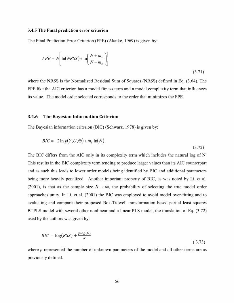
56

3.4.5 The Final prediction error criterion

The Final Prediction Error Criterion (FPE) (Akaike, 1969) is given by:

( )

−

++=

k

k

mN

mNNRSSNFPE lnln

(3.71)

where the NRSS is the Normalized Residual Sum of Squares (NRSS) defined in Eq. (3.64). The

FPE like the AIC criterion has a model fitness term and a model complexity term that influences

its value. The model order selected corresponds to the order that minimizes the FPE.

3.4.6 The Bayesian Information Criterion

The Bayesian information criterion (BIC) (Schwarz, 1978) is given by:

( ) ( )NmUYpBIC k ln,,ln2 +Θ−=

(3.72)

The BIC differs from the AIC only in its complexity term which includes the natural log of N.

This results in the BIC complexity term tending to produce larger values than its AIC counterpart

and as such this leads to lower order models being identified by BIC and additional parameters

being more heavily penalized. Another important property of BIC, as was noted by Li, et al.

(2001), is that as the sample size ù → ∞, the probability of selecting the true model order

approaches unity. In Li, et al. (2001) the BIC was employed to avoid model over-fitting and to

evaluating and compare their proposed Box-Tidwell transformation based partial least squares

BTPLS model with several other nonlinear and a linear PLS model, the translation of Eq. (3.72)

used by the authors was given by:

ü�ý = log�� + B;:��

( 3.73)

where p represented the number of unknown parameters of the model and all other terms are as

previously defined.

57

3.4.7 The Law of Iterated Logarithms Criterion

The Law of Iterated Logarithms Criterion LILC was also developed to address the problem of

model over-fitting, Hannan and Quinn (1979) proposed the following criterion:

( ) ( )NcmUYpLILC k ln,,ln2 +Θ−=

( 3.74)

where c is a multiplicative constant (>1). The constant is typically assigned a value between 2

and 4 when the information criterion is used for identifying the order of an ARMAX model. This

c term increases the complexity of identifying the true order of the model as the optimal value of

c has to be identified prior to the identification of the true order.

The previously summarized list of criterions can be categorized into a few general groups: the

first two methods are only based on evaluating model fitness while the others incorporate some

form of model complexity term. The model complexity maybe incorporated as a multiplicative

term or additive term. In the case of the last four methods on the list and the AIC criterion the

complexity term was addictive, however in the case of the Overall F-test criterion and the

adjusted multiple correlation coefficient criterion, the term was multiplicative.

3.5 Nonlinear Extension to PCA and PLS

If the underlying linear functional relationship characterizing the projection methods covered in

Chapter 2 is replaced with a non-linear function then we have a non-linear adaptation of the

traditional PLS, CCA or PCA method. Performance monitoring and prediction of process

variables for processes characterized by significant nonlinearities necessitates the use of such

nonlinear modelling methods.

Even multi-way PCA and data unfolding methods in some way seeks to mitigate for the presence

of process non-linearity by accounting for the time trajectory on the average value of the process

variable during scaling. Likewise moving window PCA and adaptive or recursive PCA (Li, et al.,

2000) takes into account the shift in the process characteristic that may occur over time.

However, with such extension to PCA described in the previous chapter, the scores or latent

variables or derived states are nonetheless linear functions of the process variables and or past

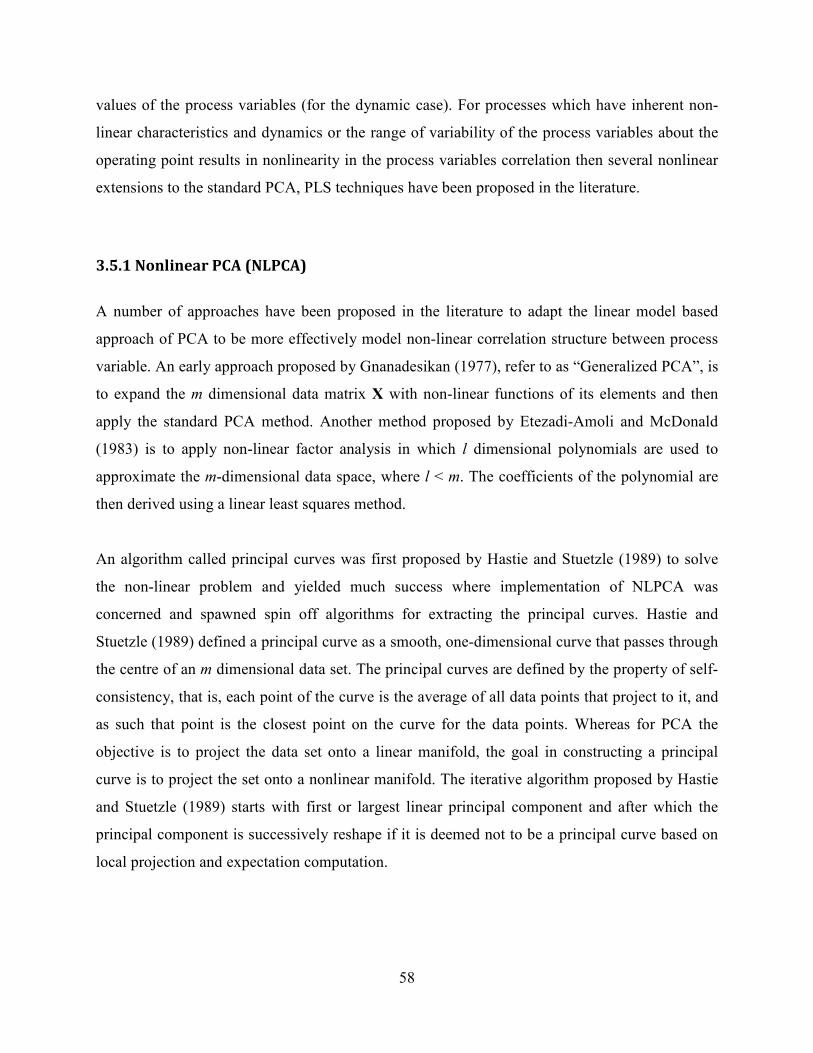
58

values of the process variables (for the dynamic case). For processes which have inherent non-

linear characteristics and dynamics or the range of variability of the process variables about the

operating point results in nonlinearity in the process variables correlation then several nonlinear

extensions to the standard PCA, PLS techniques have been proposed in the literature.

3.5.1 Nonlinear PCA (NLPCA)

A number of approaches have been proposed in the literature to adapt the linear model based

approach of PCA to be more effectively model non-linear correlation structure between process

variable. An early approach proposed by Gnanadesikan (1977), refer to as “Generalized PCA”, is

to expand the m dimensional data matrix X with non-linear functions of its elements and then

apply the standard PCA method. Another method proposed by Etezadi-Amoli and McDonald

(1983) is to apply non-linear factor analysis in which l dimensional polynomials are used to

approximate the m-dimensional data space, where l < m. The coefficients of the polynomial are

then derived using a linear least squares method.

An algorithm called principal curves was first proposed by Hastie and Stuetzle (1989) to solve

the non-linear problem and yielded much success where implementation of NLPCA was

concerned and spawned spin off algorithms for extracting the principal curves. Hastie and

Stuetzle (1989) defined a principal curve as a smooth, one-dimensional curve that passes through

the centre of an m dimensional data set. The principal curves are defined by the property of self-

consistency, that is, each point of the curve is the average of all data points that project to it, and

as such that point is the closest point on the curve for the data points. Whereas for PCA the

objective is to project the data set onto a linear manifold, the goal in constructing a principal

curve is to project the set onto a nonlinear manifold. The iterative algorithm proposed by Hastie

and Stuetzle (1989) starts with first or largest linear principal component and after which the

principal component is successively reshape if it is deemed not to be a principal curve based on

local projection and expectation computation.

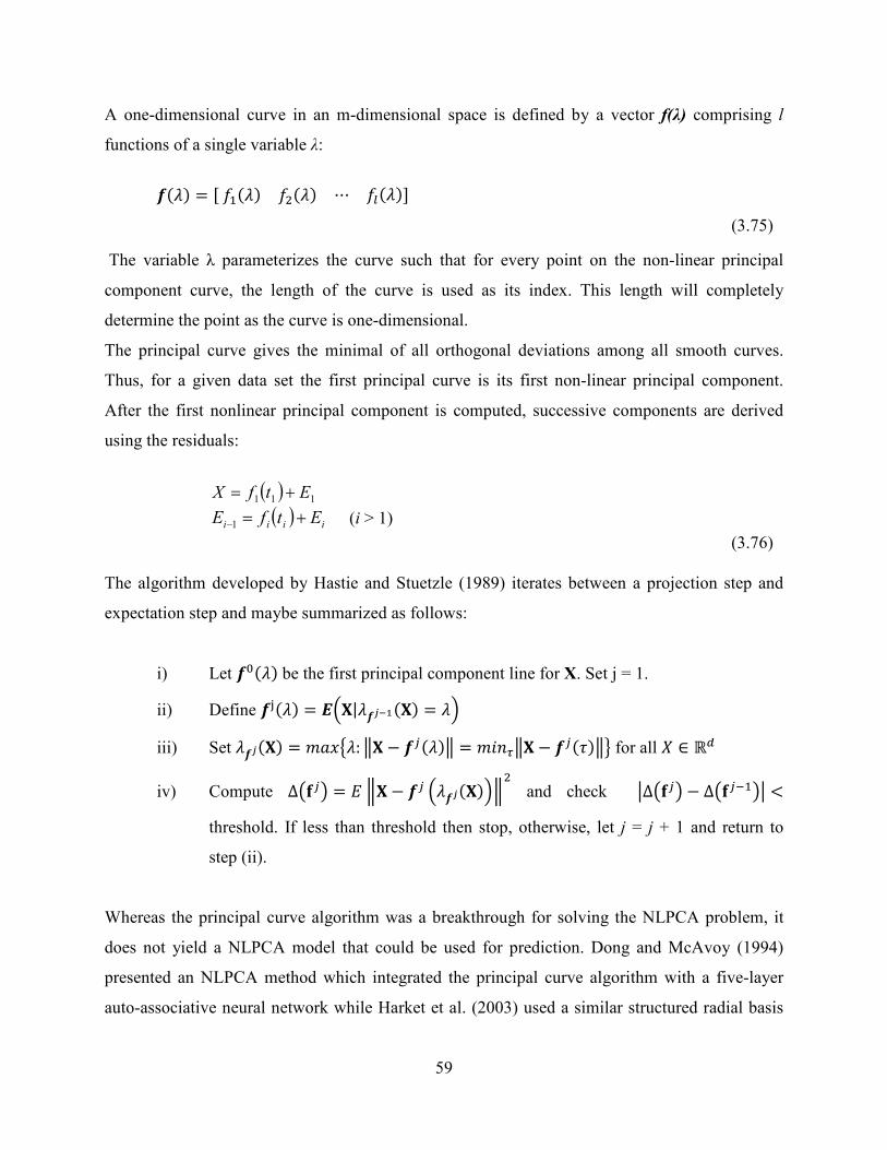
59

A one-dimensional curve in an m-dimensional space is defined by a vector f(λ) comprising l

functions of a single variable λ:

ë� = G)�1� �?� ⋯ �;� J

(3.75)

The variable λ parameterizes the curve such that for every point on the non-linear principal

component curve, the length of the curve is used as its index. This length will completely

determine the point as the curve is one-dimensional.

The principal curve gives the minimal of all orthogonal deviations among all smooth curves.

Thus, for a given data set the first principal curve is its first non-linear principal component.

After the first nonlinear principal component is computed, successive components are derived

using the residuals:

( ) 111 EtfX +=

( ) iiii EtfE +=−1 (i > 1)

(3.76)

The algorithm developed by Hastie and Stuetzle (1989) iterates between a projection step and

expectation step and maybe summarized as follows:

i) Let ëÚ� be the first principal component line for X. Set j = 1.

ii) Define ë�� = 0��ë�ç� = ��

iii) Set �ë�� = [�×�: {� − ëg� { = Ó\ {� − ëg, {Ø for all � ∈ ℝ<

iv) Compute Δf�gh = = í� − ëg ��ë�� í? and check �Δf�gh − Δf�g�1h� <

threshold. If less than threshold then stop, otherwise, let j = j + 1 and return to

step (ii).

Whereas the principal curve algorithm was a breakthrough for solving the NLPCA problem, it

does not yield a NLPCA model that could be used for prediction. Dong and McAvoy (1994)

presented an NLPCA method which integrated the principal curve algorithm with a five-layer

auto-associative neural network while Harket et al. (2003) used a similar structured radial basis

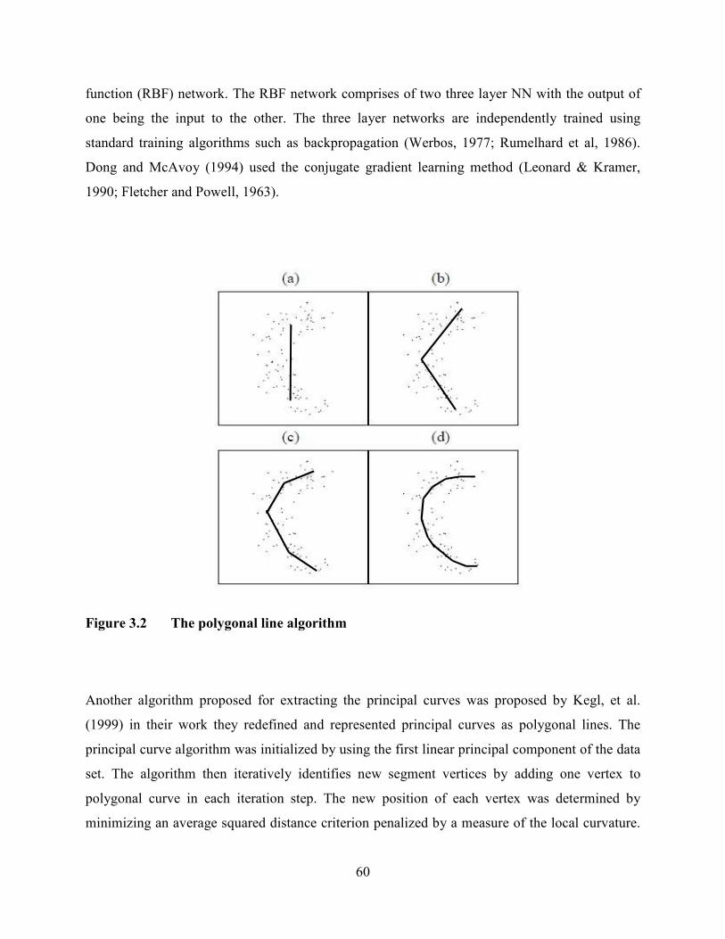
60

function (RBF) network. The RBF network comprises of two three layer NN with the output of

one being the input to the other. The three layer networks are independently trained using

standard training algorithms such as backpropagation (Werbos, 1977; Rumelhard et al, 1986).

Dong and McAvoy (1994) used the conjugate gradient learning method (Leonard & Kramer,

1990; Fletcher and Powell, 1963).

Figure 3.2 The polygonal line algorithm

Another algorithm proposed for extracting the principal curves was proposed by Kegl, et al.

(1999) in their work they redefined and represented principal curves as polygonal lines. The

principal curve algorithm was initialized by using the first linear principal component of the data

set. The algorithm then iteratively identifies new segment vertices by adding one vertex to

polygonal curve in each iteration step. The new position of each vertex was determined by

minimizing an average squared distance criterion penalized by a measure of the local curvature.

61

The stopping criterion is based on a heuristic complexity measure, determined by the number of

segments k, the dimension of data matrix, and the average squared distance of the polygonal line

from the data points. A pictorial illustration of the algorithmic process unfolding is provided in

Figure 3.2.

The algorithm was proven to be more robust than the Hastie and Stuetzle algorithm due to the

heuristics it uses to adapt the smoothing term and the number of line segments to the data. The

estimation bias is eliminated by minimizing the average distance from the curve rather than from

the vertices of the curve (this also separates it from other algorithms based on vector

quantization, such as the self-organizing map SOM or the generative topographic mapping). The

algorithm is also faster especially for large data sets.

3.5.2 Non-linear Projection to latent spaces (NLPLS)

Based on the literature reviewed, NLPLS implementations all share one thing in common, the

linear inner relationship mapping the Y scores to the X scores of the PLS algorithm is replaced

by a non-linear function:

T = XPT

+ E

(3.77)

U = YQT + F

(3.78)

U = f(T)

(3.79)

A number of different methods of defining/deriving the nonlinear inner relationship for the PLS

algorithm have been proposed in the literature:

i) Early publications of Wold, et al. (1989) and Hoskuldsson (1992) established the

framework for the quadratic nonlinear extension to the linear PLS approach. The work of

Wold, et al. (1989) was revisited by Baffi, et al. (1999b) and they recommended three

62

improvements to Wold’s algorithm to improve its applicability to modelling highly

nonlinear data sets.

ii) Wold (1992) later applied a spline function approach in which a smooth bivariate spline

function (piecewise polynomial functions - quadratic or cubic) was applied as the inner

relation to fit a nonlinear mapping between the pair of latent variables. The spline

function approach provided more generality and flexibility in defining the non-linear

relationship of the inner relationship than the QPLS approach (Wold, et al., 1989).

However, both these approaches are essentially a pseudo-linear fit and in the case of a

defining a complicated nonlinear relationship, nonlinear parameter estimation would be

required. Li, et al. (1999) therefore proposed combining an efficient nonlinear parameter

estimation algorithm in the form of a numeric genetic algorithm within the nonlinear PLS

algorithm. Identifying that the adaptation of the linear PLS weight selection process was

a critical issue for the different non-linear PLS methods, Hassel et al. (2001) proposed an

estimation of the weight vector based upon the principle of weighted averages and

reciprocal variance criterion.

iii) Qin and McAvoy (1992) generalized the PLS model to a nonlinear framework by

imbedding feedforward neural networks into PLS modelling. The feedforward network

implementation developed a single feedforward network to map the inner relations

between each pair of scores generated sequentially. As such this approach decomposed

the multivariate regression problem into a number of univariate nonlinear regressors.

Malthouse, et al. (1997) conducted simulation exercises to compare the NLPLS

feedforward model with pursuit regression based and neural network modelling

approaches and concluded that NLPLS did give much advantage over other projection-

based algorithms such as pursuit regression based algorithms and neural networks. Apart

from feedforward networks other neural networks can be applied to map the non-linear

relationship, such as radial basis networks, see Baffi, et al. (1999a). However, RBF

networks are considered superior to the sigmoidal feedforward networks because the

training is simpler and faster. The NN approach has been demonstrated to provide a

stable and generic (no prior assumption is made about the nonlinear nature of the process)

modelling tool.

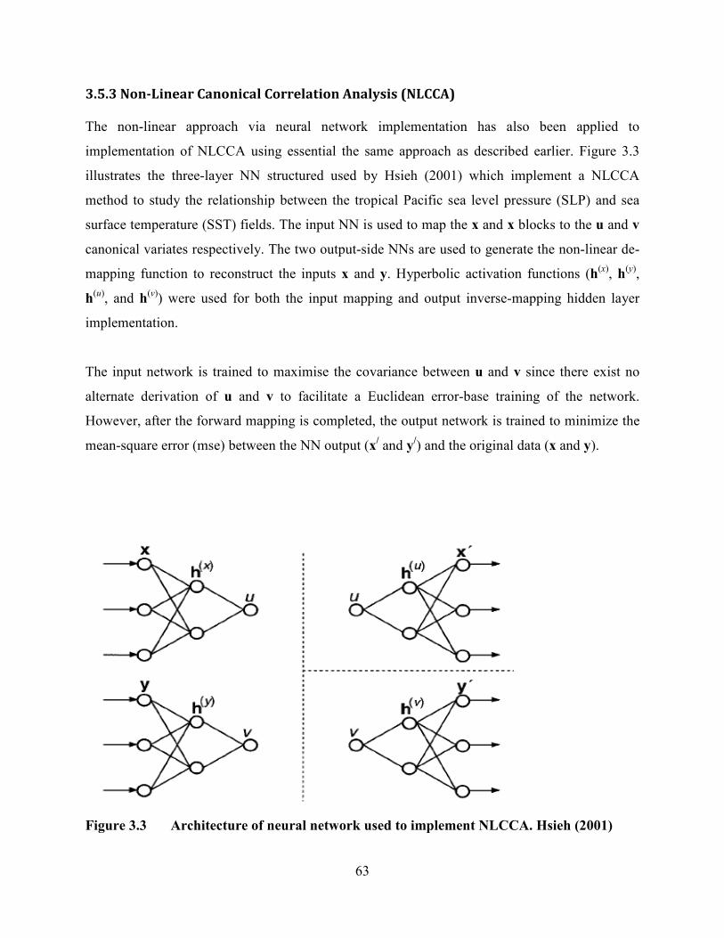
63

3.5.3 Non-Linear Canonical Correlation Analysis (NLCCA)

The non-linear approach via neural network implementation has also been applied to

implementation of NLCCA using essential the same approach as described earlier. Figure 3.3

illustrates the three-layer NN structured used by Hsieh (2001) which implement a NLCCA

method to study the relationship between the tropical Pacific sea level pressure (SLP) and sea

surface temperature (SST) fields. The input NN is used to map the x and x blocks to the u and v

canonical variates respectively. The two output-side NNs are used to generate the non-linear de-

mapping function to reconstruct the inputs x and y. Hyperbolic activation functions (h(x)

, h(y)

,

h(u)

, and h(v)

) were used for both the input mapping and output inverse-mapping hidden layer

implementation.

The input network is trained to maximise the covariance between u and v since there exist no

alternate derivation of u and v to facilitate a Euclidean error-base training of the network.

However, after the forward mapping is completed, the output network is trained to minimize the

mean-square error (mse) between the NN output (x/ and y

/) and the original data (x and y).

Figure 3.3 Architecture of neural network used to implement NLCCA. Hsieh (2001)

64

3.6 Hybrid Data Driven/ Mechanistic Model based Approaches

Prior to the proliferation of the data based black-box models for process modelling, first

principle mechanistic models were used to determine whether a process was operating desirably.

Mechanistic models are particularly appealing because of the following reasons:

i) The challenges of making process monitoring more robust and reliable especially for

dynamic and or highly non-linear processes could be improved if known chemical

and physical relationships about the process could be incorporated in the process

monitoring scheme.

ii) Mechanistic models based upon actual chemistry and design of the process affords

tracing and understanding of the nature and source of process upsets to be linked to

specific process variables or unit operations.

iii) Data based black-box models do not give much insight into the underlying process

behaviours and diagnosis and interpretation of process upset can be subjective.

Improving the reliability and confidence in the diagnosis maybe accomplished by the

inclusion of known and designed relationship existing between the process variables.

One of the methods that have been explored briefly in the literature to combat and address the

issue of providing robust reliable monitoring of non-linear batch and continuous processes

characterized by grade changes is model-based PCA proposed by Wachs and Lewin (1999). This

was one of the earliest published papers in which the concept of combining a first principle

mechanistic model of the process with a database statistical model was explored. The concept

which is illustrated in Figure 3.4 is premised on existence of a first principle model of the

process which is sufficiently accurate such that the process non-linearity characteristic and

whatever serial correlation that exist between the process variables are captured. Then the

process of subtracting the model outputs from the real plant data would result in residuals free of

non-linearity and autocorrelation. The residuals could therefore be treated using any standard

linear statistical multivariate technique such as PCA.

In theory a perfect model would result in the residuals being essentially white noise and as such

any process disturbance, faulty sensor, or equipment failure would manifest itself in the residual

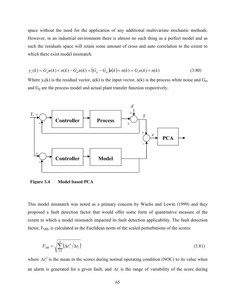
65

space without the need for the application of any additional multivariate stochastic methods.

However, in an industrial environment there is almost no such thing as a perfect model and as

such the residuals space will retain some amount of cross and auto correlation to the extent to

which there exist model mismatch:

( ) ( ) )()()()()()()( knkuGknkuGGkuGknkuGky empmpe +=+−=−+= (3.80)

Where ye(k) is the residual vector, u(k) is the input vector, n(k) is the process white noise and Gm

and Gp are the process model and actual plant transfer function respectively.

This model mismatch was noted as a primary concern by Wachs and Lewin (1999) and they

proposed a fault detection factor that would offer some form of quantitative measure of the

extent to which a model mismatch impacted its fault detection applicability. The fault detection

factor, FMB, is calculated as the Euclidean norm of the scaled perturbations of the scores:

( )∑=

∆∆=k

i

i

d

iMB ttF1

(3.81)

where d

it∆ is the mean in the scores during normal operating condition (NOC) to its value when

an alarm is generated for a given fault, and it∆ is the range of variability of the score during

Controller

Process

Controller

PCA

Model

+

-

+

-

+

-

+

+

d

e

Y Ys

Figure 3.4 Model based PCA

66

normal operating condition. The more detectable a disturbances is or unaffected by model

uncertainty then the greater FMB is. Values of FMB < 1 indicate faults that are difficult to detect.

Another measure of model mismatch measurement suggested in a publication by Rotem et al.

(2000) is to apply the Durbin-Watson test to elucidate the autocorrelation retained in the

residuals:

[ ]

( )∑

∑

=

+

=

−−=

n

k

n

k

ke

keke

1

2

1

2

2)1()(

ρ

(3.82) where e(k) and e(k-1) are the sample residuals one time sample apart.

If the numerator term is expanded, then the following is obtained:

( )[ ]∑=

−+−−n

k

kekekeke2

22)1()1()(2

(3.83)

and if the samples are uncorrelated then ( ) ( )∑∑+

=

+

=

−=1

2

21

2

21

n

i

n

i

keke and the summation of the product

term should tend to zero and hence ρ tends to a value of 2. Positive autocorrelation would be

indicated in the range of 0 ≤ ρ < 2 and negative autocorrelation would give values in the range

2 < ρ ≤ 4.

Recognising the limitations of model-based PCA in that unless the model was a perfect one, the

residuals could still retain serial and autocorrelation structure, McPherson, et al. (2002) proposed

a super-model based approach to monitoring of batch processes. The concept is illustrated in

Figure 3.5 and the idea behind it is that an additional stage (error model) would be incorporated

to augment the mechanistic plant model to end of removing whatever remaining structure that

may exist in the first stage residuals.

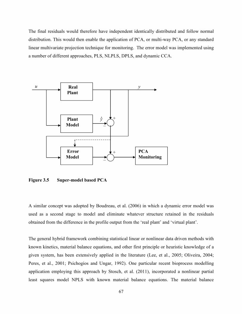
67

The final residuals would therefore have independent identically distributed and follow normal

distribution. This would then enable the application of PCA, or multi-way PCA, or any standard

linear multivariate projection technique for monitoring. The error model was implemented using

a number of different approaches, PLS, NLPLS, DPLS, and dynamic CCA.

Figure 3.5 Super-model based PCA

A similar concept was adopted by Boudreau, et al. (2006) in which a dynamic error model was

used as a second stage to model and eliminate whatever structure retained in the residuals

obtained from the difference in the profile output from the ‘real plant’ and ‘virtual plant’.

The general hybrid framework combining statistical linear or nonlinear data driven methods with

known kinetics, material balance equations, and other first principle or heuristic knowledge of a

given system, has been extensively applied in the literature (Lee, et al., 2005; Oliveira, 2004;

Peres, et al., 2001; Psichogios and Ungar, 1992). One particular recent bioprocess modelling

application employing this approach by Stosch, et al. (2011), incorporated a nonlinear partial

least squares model NPLS with known material balance equations. The material balance

Real

Plant

Plant

Model

Error

Model

PCA

Monitoring

u y

+

_

+

_

68

equations were used to capture the dynamics of the bioprocess – both the cellular and bioreactor

system. The model was evaluated on a fed-batch production of a recombinant protein –

Bordetella Pertussis batch cultivation and demonstrated better prediction accuracy over

alternative non-hybrid approaches at implementing a dynamic model.

Hybrid approaches involving the integration of different statistical data driven modeling

techniques are also quite common in the literature. Yan (2010) developed a soft sensor for

detection of naptha dry point using an Hybrid Artificial Neural Network HANN. The HANN

network employed a partial least square regression PLSR model to remove the multicolinearity

among the hidden layer neuron outputs and to enhance the relational model between the hidden

and output layer neuron outputs.

3.7 Summary

Three subspace method were reviewed – CVA, N4SID and MOESP. The literature review

sought to identify the commons traits of each of the three subspace method in terms of the

central objective of representing a data set in a lower order dimensional space. The differences

were also highlighted and suitability of the CVA method for process monitoring applications

based upon comparative studies conducted by several researchers was the motivating factor to

pursue and a proposed a CVA state space model based dynamic modelling approach in this

thesis.

The review also explored a number of successfully proposed methods of adapting linear

statistical methods of PCA and PLS to tackle nonlinear process modelling and monitoring

applications. More specifically, several algorithmic approaches to implementing principle curves

in the case of NLPCA were reviewed. The review also covered several methods of modifying the

linear PLS algorithm to incorporate a neural network based or polynomial inner relationship.

Several hybrid model based approaches for prediction and performance monitoring across both

batch and continuous processes were reviewed. The class of hybrid models included those

combining mechanistic (first principle model) with data driven model based approaches and

69

those non-mechanistic approach combining statistical data driven methods of different paradigms

such as linear versus nonlinear data based modelling techniques.

70

Chapter 4 : A Simplified CVA State Space Modelling

Approach for Process-Monitoring Specific Applications

4.1 Introduction

The use of state space models for the modelling, control and monitoring of dynamic

processes have been reported to be superior to other multivariate statistical methods. In the area

of system identification and predictive modelling, Juricek, et al. (2005) demonstrated that

subspace models based on canonical variate analysis (CVA) and numerical algorithm for

subspace identification (N4SID) outperformed regression models based on partial least squares

(PLS) and constraint categorical regression (CCR). They also demonstrated that of the two

subspace modelling methods, the CVA model was more accurate than its N4SID counterpart.

Other comparative analysis works carried out by Simoglou, et al. (1999a) and Negiz and Cinar

(1997b) have also provided support for the superior performance of CVA based state space

models .

A few variants of the state space model representations have also been explored and presented on

in the literature. Typically, the form of CVA based state-space representation is one that can be

used in applications ranging from process modelling, control and monitoring. Such a model

generally requires the estimation of five matrices to fully parameterize the model. In control

system applications the representation is necessary, as control of the plant is achieved via

71

methods involving the application of calculated input signal(s) based upon the past output

measurements. Thus far very little emphasis has been placed on selecting a state-space model

based upon its intended application and most if not all recent papers employing state space

models for process monitoring applications have resorted to this full model representation (Lee,

et al., 2006; Yao and Gao, 2008; Odiowei and Cao, 2010).

An adaptation of the state-space model representation and CVA based derivation for the specific

purpose of process monitoring is proposed in this chapter. The proposed state space model

employs a significantly reduced number of parameters. The reduced dimensionality of the model

in conjunction with a slightly amended method of constructing the past vector, provides for a

much simpler and more efficient stochastic estimation method for deriving the state matrices.

Using the benchmark Tennessee Eastman processor simulator under close-loop control, a

comprehensive fault detection analysis is carried out using the Hotelling’s T2 statistics and

squared prediction error (Q) statistics of the state and output residuals. The results were

compared with reported fault detection performance from previous publications (Russell, et al.,

2000; Detroja, et al., 2007), both of papers published fault detection results on the same set of 21

faults reviewed in this paper. Russell, et al. (2000) evaluated three different fault detection

models: the traditional CVA state space modelling technique, standard and dynamic principal

component analysis (D)PCA. While Detroja, et al. (2007) evaluated the detection performance of

the Hotelling’s T2 statistics and Q statistics based upon a statistical method called

correspondence analysis (CA). The results from these previous publications points to the

traditional CVA state space model being overall the best performing model. The results of this

research demonstrates that the proposed CVA state space model can offer at least the same and

in some cases better fault detection capabilities in terms of detection delay time when compared

with the fault detection performance of the traditional CVA state space model.

The chapter is organised as follows: Section 4.2 highlights the differences between the proposed

state space model and state variable derivation with that of the models and methods pioneered by

Larimore (Larimore, 1990) and reviewed in Chapter 3. Section 4.3 delves into the application of

several model selection criterions and how they were employed for the selection of the

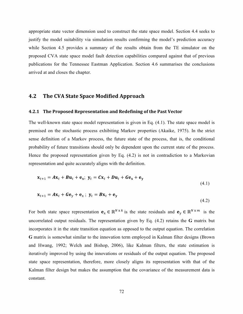
72

appropriate state vector dimension used to construct the state space model. Section 4.4 seeks to

justify the model suitability via simulation results confirming the model’s prediction accuracy

while Section 4.5 provides a summary of the results obtain from the TE simulator on the

proposed CVA state space model fault detection capabilities compared against that of previous

publications for the Tennessee Eastman Application. Section 4.6 summarises the conclusions

arrived at and closes the chapter.

4.2 The CVA State Space Modified Approach

4.2.1 The Proposed Representation and Redefining of the Past Vector

The well-known state space model representation is given in Eq. (4.1). The state space model is

premised on the stochastic process exhibiting Markov properties (Akaike, 1975). In the strict

sense definition of a Markov process, the future state of the process, that is, the conditional

probability of future transitions should only be dependent upon the current state of the process.

Hence the proposed representation given by Eq. (4.2) is not in contradiction to a Markovian

representation and quite accurately aligns with the definition.

p��1 = !p� + j�� + �p; �� = �p� + �� + ��p + ��

(4.1)

p��1 = !p� + �� + �� ; �� = jp� + ��

(4.2)

For both state space representation �� ∈ ℝ�)�)^)is the state residuals and �� ∈ ℝ�)�)@) is the

uncorrelated output residuals. The representation given by Eq. (4.2) retains the G matrix but

incorporates it in the state transition equation as opposed to the output equation. The correlation

G matrix is somewhat similar to the innovation term employed in Kalman filter designs (Brown

and Hwang, 1992; Welch and Bishop, 2006), like Kalman filters, the state estimation is

iteratively improved by using the innovations or residuals of the output equation. The proposed

state space representation, therefore, more closely aligns its representation with that of the

Kalman filter design but makes the assumption that the covariance of the measurement data is

constant.

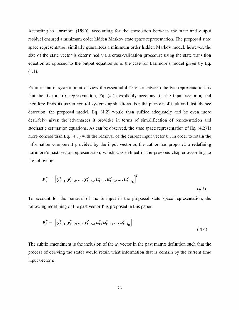
73

According to Larimore (1990), accounting for the correlation between the state and output

residual ensured a minimum order hidden Markov state space representation. The proposed state

space representation similarly guarantees a minimum order hidden Markov model, however, the

size of the state vector is determined via a cross-validation procedure using the state transition

equation as opposed to the output equation as is the case for Larimore’s model given by Eq.

(4.1).

From a control system point of view the essential difference between the two representations is

that the five matrix representation, Eq. (4.1) explicitly accounts for the input vector ut and

therefore finds its use in control systems applications. For the purpose of fault and disturbance

detection, the proposed model, Eq. (4.2) would then suffice adequately and be even more

desirably, given the advantages it provides in terms of simplification of representation and

stochastic estimation equations. As can be observed, the state space representation of Eq. (4.2) is

more concise than Eq. (4.1) with the removal of the current input vector ut. In order to retain the

information component provided by the input vector ut the author has proposed a redefining

Larimore’s past vector representation, which was defined in the previous chapter according to

the following:

H�� =) ¡¢��1� , ¢��?� , … . ¢��;£� , _��1� , _��?� , … . _��;¤� ¥�

(4.3)

To account for the removal of the ut input in the proposed state space representation, the

following redefining of the past vector P is proposed in this paper:

H�� =) ¡¢��1� , ¢��?� , … . ¢��;£� , _�� , _��1� , … . _��;¤� ¥�

( 4.4)

The subtle amendment is the inclusion of the ut vector in the past matrix definition such that the

process of deriving the states would retain what information that is contain by the current time

input vector ut.

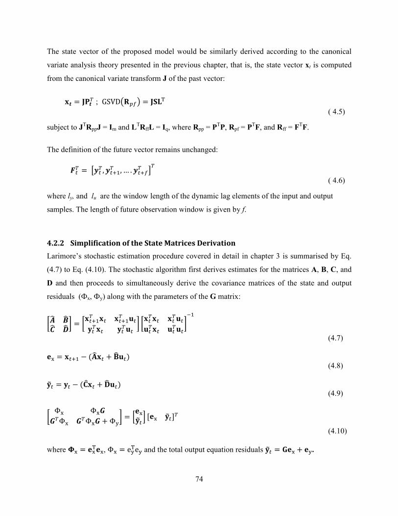
74

The state vector of the proposed model would be similarly derived according to the canonical

variate analysis theory presented in the previous chapter, that is, the state vector xt is computed

from the canonical variate transform J of the past vector:

p2 = �M2� ; GSVDfiB¦h = ��

( 4.5)

subject to JTRppJ = Im and L

TRffL = Iq, where Rpp = P

TP, Rpf = P

TF, and Rff = F

TF.

The definition of the future vector remains unchanged:

`�� =) A¢�� , ¢��1� , … . ¢��¦� C�

( 4.6)

where ly, and lu are the window length of the dynamic lag elements of the input and output

samples. The length of future observation window is given by f.

4.2.2 Simplification of the State Matrices Derivation

Larimore’s stochastic estimation procedure covered in detail in chapter 3 is summarised by Eq.

(4.7) to Eq. (4.10). The stochastic algorithm first derives estimates for the matrices A, B, C, and

D and then proceeds to simultaneously derive the covariance matrices of the state and output

residuals (Фx, Фy) along with the parameters of the G matrix:

º!w jw�w �w½ = ºp��1� p� p��1� ��p� �� ½ ºp��p� p��p� ��½

�1

(4.7)

�� = p��1 − �wp� + Åw��

(4.8)

�� = �� − »¼p� + Çw��

(4.9)

º Φ� Φ��Φ� ��Φ��+Φ�½ = ¡�� ¥ G�� J�

(4.10)

where Æ� = ��, Φ� = e��e� and the total output equation residuals �� = Ò�� + ��.

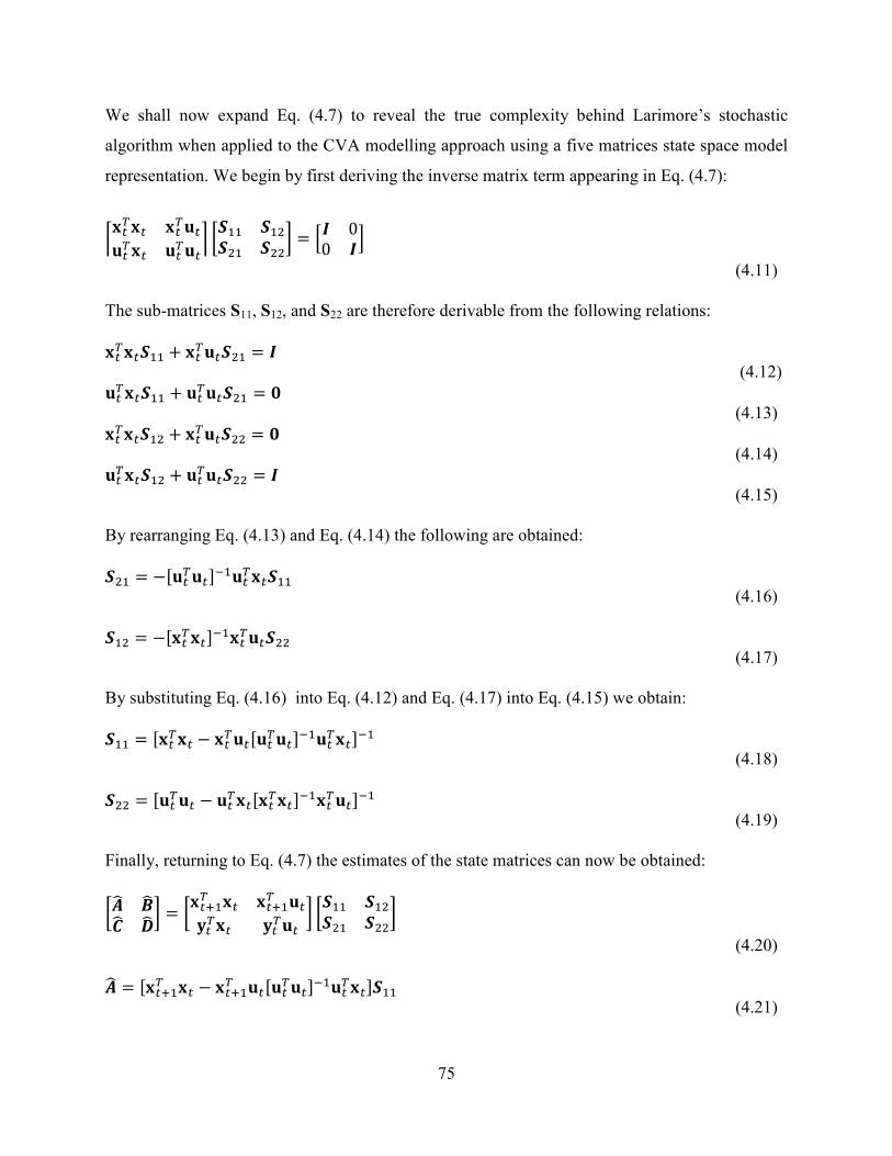
75

We shall now expand Eq. (4.7) to reveal the true complexity behind Larimore’s stochastic

algorithm when applied to the CVA modelling approach using a five matrices state space model

representation. We begin by first deriving the inverse matrix term appearing in Eq. (4.7):

�p��p� p��p� �� ºô11 ô1?ô?1 ô??½ = ¡z 00 z¥

(4.11)

The sub-matrices S11, S12, and S22 are therefore derivable from the following relations:

p��p�ô11 + p��ô?1 = z (4.12) ��p�ô11 + ��ô?1 = â

(4.13) p��p�ô1? + p��ô?? = â (4.14) ��p�ô1? + ��ô?? = z

(4.15)

By rearranging Eq. (4.13) and Eq. (4.14) the following are obtained:

ô?1 = −G��J�1��p�ô11 (4.16)

ô1? = −Gp��p�J�1p��ô?? (4.17)

By substituting Eq. (4.16) into Eq. (4.12) and Eq. (4.17) into Eq. (4.15) we obtain:

ô11 = Gp��p� − p��G��J�1��p�J�1 (4.18)

ô?? = G�� − ��p�Gp��p�J�1p��J�1 (4.19)

Finally, returning to Eq. (4.7) the estimates of the state matrices can now be obtained:

º!w jw�w �w½ = ºp��1� p� p��1� ��p� �� ½ ºô11 ô1?ô?1 ô??½

(4.20)

!w = Gp��1� p� − p��1� ��G��J�1��p�Jô11

(4.21)

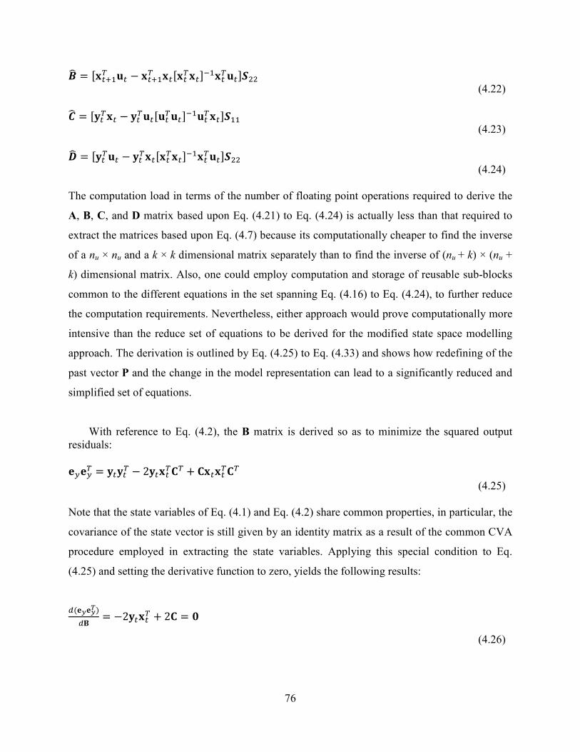
76

jw = Gp��1� �� − p��1� p�Gp��p�J�1p��Jô??

(4.22)

�w = G��p� − ��G��J�1��p�Jô11 (4.23)

�w = G�� − ��p�Gp��p�J�1p��Jô?? (4.24)

The computation load in terms of the number of floating point operations required to derive the

A, B, C, and D matrix based upon Eq. (4.21) to Eq. (4.24) is actually less than that required to

extract the matrices based upon Eq. (4.7) because its computationally cheaper to find the inverse

of a nu × nu and a k × k dimensional matrix separately than to find the inverse of (nu + k) × (nu +

k) dimensional matrix. Also, one could employ computation and storage of reusable sub-blocks

common to the different equations in the set spanning Eq. (4.16) to Eq. (4.24), to further reduce

the computation requirements. Nevertheless, either approach would prove computationally more

intensive than the reduce set of equations to be derived for the modified state space modelling

approach. The derivation is outlined by Eq. (4.25) to Eq. (4.33) and shows how redefining of the

past vector P and the change in the model representation can lead to a significantly reduced and

simplified set of equations.

With reference to Eq. (4.2), the B matrix is derived so as to minimize the squared output

residuals:

�� = �� − 2��p��»� + »p�p��»�

(4.25)

Note that the state variables of Eq. (4.1) and Eq. (4.2) share common properties, in particular, the

covariance of the state vector is still given by an identity matrix as a result of the common CVA

procedure employed in extracting the state variables. Applying this special condition to Eq.

(4.25) and setting the derivative function to zero, yields the following results:

<�£�£� <Å = −2��p�� + 2» = â)

(4.26)

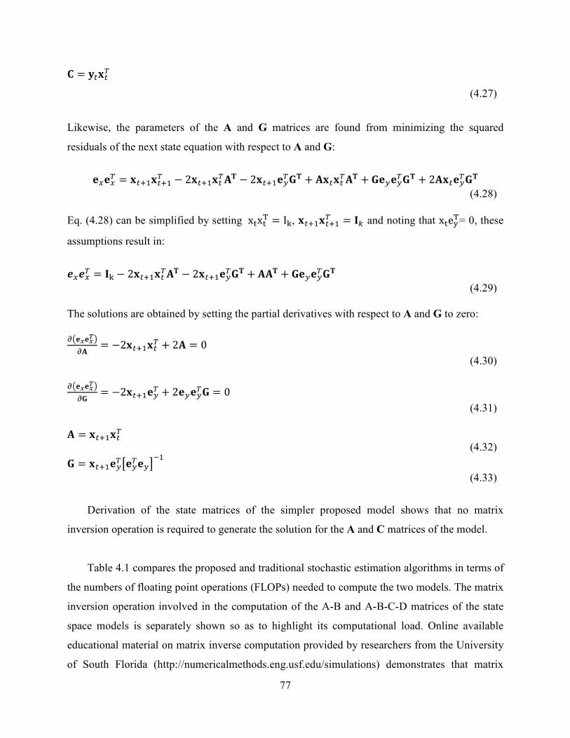
77

» = ��p��

(4.27)

Likewise, the parameters of the A and G matrices are found from minimizing the squared

residuals of the next state equation with respect to A and G:

�� = p��1p��1� − 2p��1p�� − 2p��1��Ò� + �p�p�� + Ò��Ò� + 2�p��Ò�

(4.28)

Eq. (4.28) can be simplified by setting )x¹x¹� = I�, p��1p��1� = #^ and noting that x¹e��= 0, these

assumptions result in:

q�q�� = #� − 2p��1p�� − 2p��1��Ò� + �� + Ò��Ò�

(4.29)

The solutions are obtained by setting the partial derivatives with respect to A and G to zero:

�f��h

�� = −2p��1p�� + 2� = 0

(4.30)

�f��h

�Ò = −2p��1�� + 2��Ò = 0

(4.31)

� = p��1p�� (4.32) Ò = p��1��A��C�1

(4.33)

Derivation of the state matrices of the simpler proposed model shows that no matrix

inversion operation is required to generate the solution for the A and C matrices of the model.

Table 4.1 compares the proposed and traditional stochastic estimation algorithms in terms of

the numbers of floating point operations (FLOPs) needed to compute the two models. The matrix

inversion operation involved in the computation of the A-B and A-B-C-D matrices of the state

space models is separately shown so as to highlight its computational load. Online available

educational material on matrix inverse computation provided by researchers from the University

of South Florida (http://numericalmethods.eng.usf.edu/simulations) demonstrates that matrix

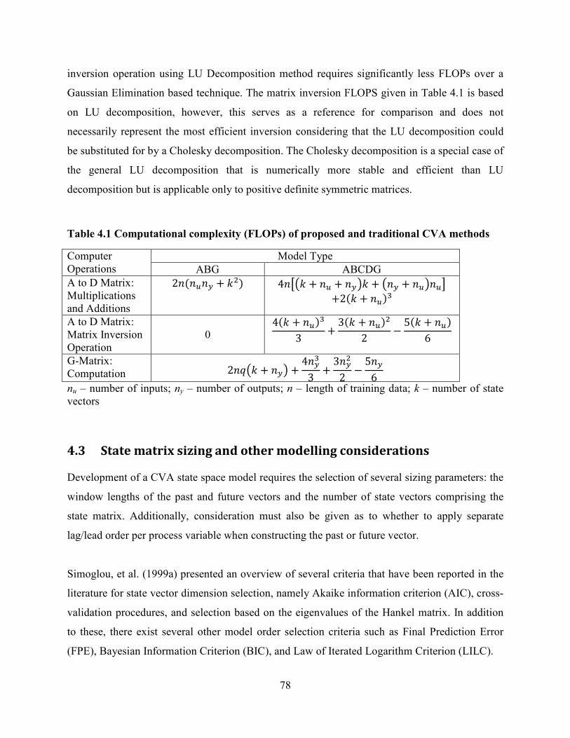
78

inversion operation using LU Decomposition method requires significantly less FLOPs over a

Gaussian Elimination based technique. The matrix inversion FLOPS given in Table 4.1 is based

on LU decomposition, however, this serves as a reference for comparison and does not

necessarily represent the most efficient inversion considering that the LU decomposition could

be substituted for by a Cholesky decomposition. The Cholesky decomposition is a special case of

the general LU decomposition that is numerically more stable and efficient than LU

decomposition but is applicable only to positive definite symmetric matrices.

Table 4.1 Computational complexity (FLOPs) of proposed and traditional CVA methods

Computer

Operations

Model Type

ABG ABCDG

A to D Matrix:

Multiplications

and Additions

2\\î\� + �? 4\Af� + \î + \�h� + f\� + \îh\îC +2� + \î �

A to D Matrix:

Matrix Inversion

Operation

0 4� + \î �

3 + 3� + \î ?2 − 5� + \î 6

G-Matrix:

Computation 2\$f� + \�h + 4\��3 + 3\�?2 − 5\�

6

nu – number of inputs; ny – number of outputs; n – length of training data; k – number of state

vectors

4.3 State matrix sizing and other modelling considerations

Development of a CVA state space model requires the selection of several sizing parameters: the

window lengths of the past and future vectors and the number of state vectors comprising the

state matrix. Additionally, consideration must also be given as to whether to apply separate

lag/lead order per process variable when constructing the past or future vector.

Simoglou, et al. (1999a) presented an overview of several criteria that have been reported in the

literature for state vector dimension selection, namely Akaike information criterion (AIC), cross-

validation procedures, and selection based on the eigenvalues of the Hankel matrix. In addition

to these, there exist several other model order selection criteria such as Final Prediction Error

(FPE), Bayesian Information Criterion (BIC), and Law of Iterated Logarithm Criterion (LILC).

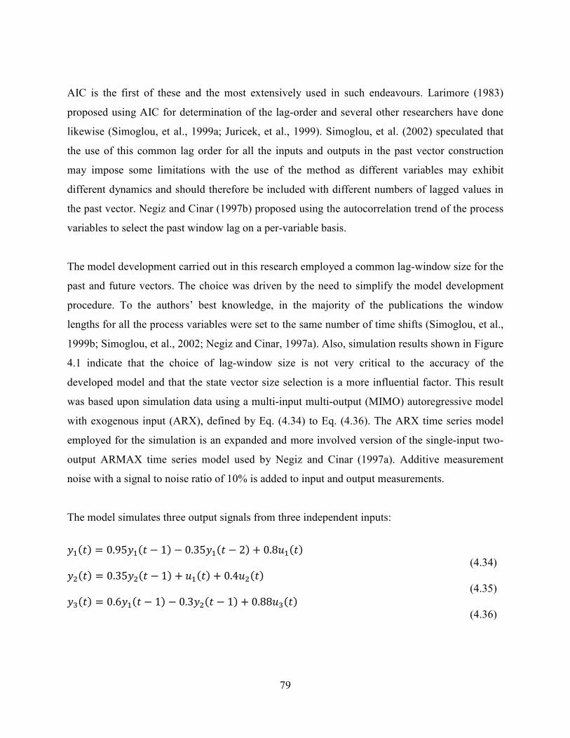
79

AIC is the first of these and the most extensively used in such endeavours. Larimore (1983)

proposed using AIC for determination of the lag-order and several other researchers have done

likewise (Simoglou, et al., 1999a; Juricek, et al., 1999). Simoglou, et al. (2002) speculated that

the use of this common lag order for all the inputs and outputs in the past vector construction

may impose some limitations with the use of the method as different variables may exhibit

different dynamics and should therefore be included with different numbers of lagged values in

the past vector. Negiz and Cinar (1997b) proposed using the autocorrelation trend of the process

variables to select the past window lag on a per-variable basis.

The model development carried out in this research employed a common lag-window size for the

past and future vectors. The choice was driven by the need to simplify the model development

procedure. To the authors’ best knowledge, in the majority of the publications the window

lengths for all the process variables were set to the same number of time shifts (Simoglou, et al.,

1999b; Simoglou, et al., 2002; Negiz and Cinar, 1997a). Also, simulation results shown in Figure

4.1 indicate that the choice of lag-window size is not very critical to the accuracy of the

developed model and that the state vector size selection is a more influential factor. This result

was based upon simulation data using a multi-input multi-output (MIMO) autoregressive model

with exogenous input (ARX), defined by Eq. (4.34) to Eq. (4.36). The ARX time series model

employed for the simulation is an expanded and more involved version of the single-input two-

output ARMAX time series model used by Negiz and Cinar (1997a). Additive measurement

noise with a signal to noise ratio of 10% is added to input and output measurements.

The model simulates three output signals from three independent inputs:

%1Y = 0.95%1Y − 1 − 0.35%1Y − 2 + 0.8Û1Y (4.34)

%?Y = 0.35%?Y − 1 + Û1Y + 0.4Û?Y (4.35)

%�Y = 0.6%1Y − 1 − 0.3%?Y − 1 + 0.88Û�Y (4.36)

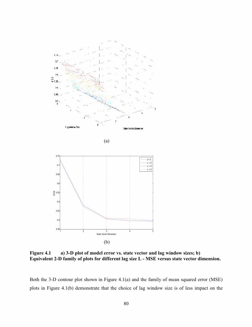
80

(a)

(b)

Figure 4.1 a) 3-D plot of model error vs. state vector and lag window sizes; b)

Equivalent 2-D family of plots for different lag size L - MSE versus state vector dimension.

Both the 3-D contour plot shown in Figure 4.1(a) and the family of mean squared error (MSE)

plots in Figure 4.1(b) demonstrate that the choice of lag window size is of less impact on the

1 2 3 4 50.35

0.4

0.45

0.5

0.55

0.6

0.65

0.7

0.75

State Vector Dimension

MSE

L= 2

L = 3

L = 4

L = 5

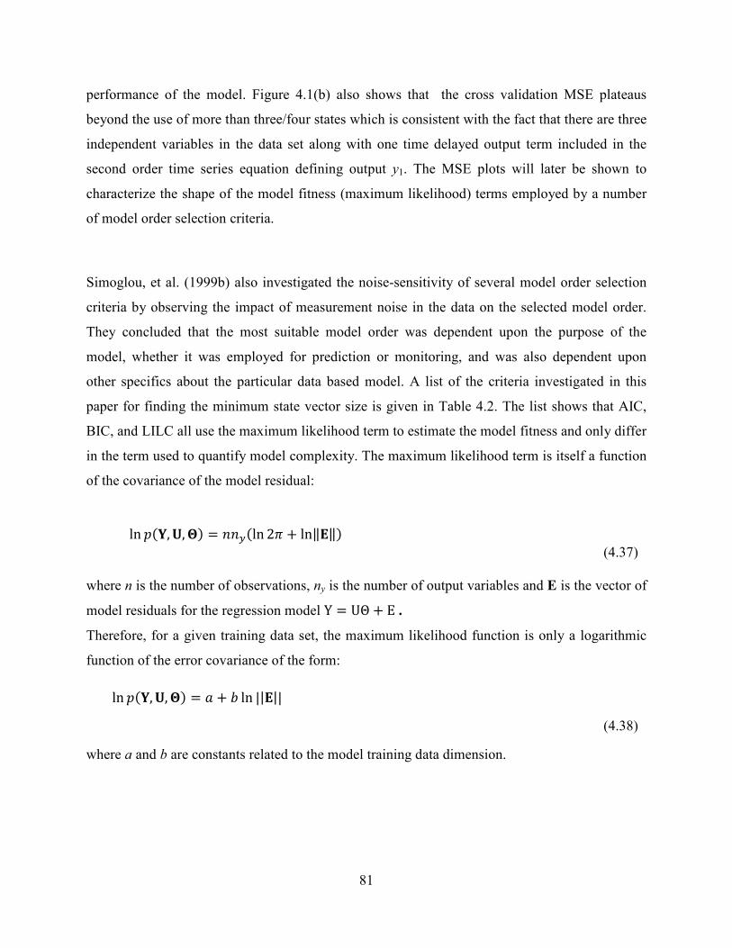
81

performance of the model. Figure 4.1(b) also shows that the cross validation MSE plateaus

beyond the use of more than three/four states which is consistent with the fact that there are three

independent variables in the data set along with one time delayed output term included in the

second order time series equation defining output y1. The MSE plots will later be shown to

characterize the shape of the model fitness (maximum likelihood) terms employed by a number

of model order selection criteria.

Simoglou, et al. (1999b) also investigated the noise-sensitivity of several model order selection

criteria by observing the impact of measurement noise in the data on the selected model order.

They concluded that the most suitable model order was dependent upon the purpose of the

model, whether it was employed for prediction or monitoring, and was also dependent upon

other specifics about the particular data based model. A list of the criteria investigated in this

paper for finding the minimum state vector size is given in Table 4.2. The list shows that AIC,

BIC, and LILC all use the maximum likelihood term to estimate the model fitness and only differ

in the term used to quantify model complexity. The maximum likelihood term is itself a function

of the covariance of the model residual:

ln )O,P, ñ = \\�ln2* + lnZNZ

(4.37)

where n is the number of observations, ny is the number of output variables and E is the vector of

model residuals for the regression model Y = UΘ + E .

Therefore, for a given training data set, the maximum likelihood function is only a logarithmic

function of the error covariance of the form:

ln )O,P, ñ = [ + c ln ��N��))

(4.38)

where a and b are constants related to the model training data dimension.

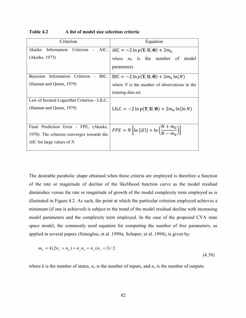
82

Table 4.2 A list of model size selection criteria

Criterion Equation

Akaike Information Criterion - AIC,

(Akaike, 1973)

AIC = −2 ln )O,P, ñ + 2^

where mk is the number of model

parameters

Bayesian Information Criterion - BIC,

(Hannan and Quinn, 1979)

BIC = −2 ln)O, P, ñ + 2^ lnù where N is the number of observations in the

training data set

Law of Iterated Logarithm Criterion - LILC,

(Hannan and Quinn, 1979)

LILC = −2 ln )O,P, ñ + 2^ lnlnù Final Prediction Error - FPE, (Akaike,

1970). The criterion converges towards the

AIC for large values of N.

34= = ù ºln ��=��+ ln éù +^ù −^ê½

The desirable parabolic shape obtained when these criteria are employed is therefore a function

of the rate or magnitude of decline of the likelihood function curve as the model residual

diminishes versus the rate or magnitude of growth of the model complexity term employed as is

illustrated in Figure 4.2. As such, the point at which the particular criterion employed achieves a

minimum (if one is achieved) is subject to the trend of the model residual decline with increasing

model parameters and the complexity term employed. In the case of the proposed CVA state

space model, the commonly used equation for computing the number of free parameters, as

applied in several papers (Simoglou, et al. 1999a; Schaper, et al. 1994), is given by:

2/)1()2( ++++= yyuyuyk nnnnnnkm

(4.39)

where k is the number of states, nu is the number of inputs, and ny is the number of outputs.

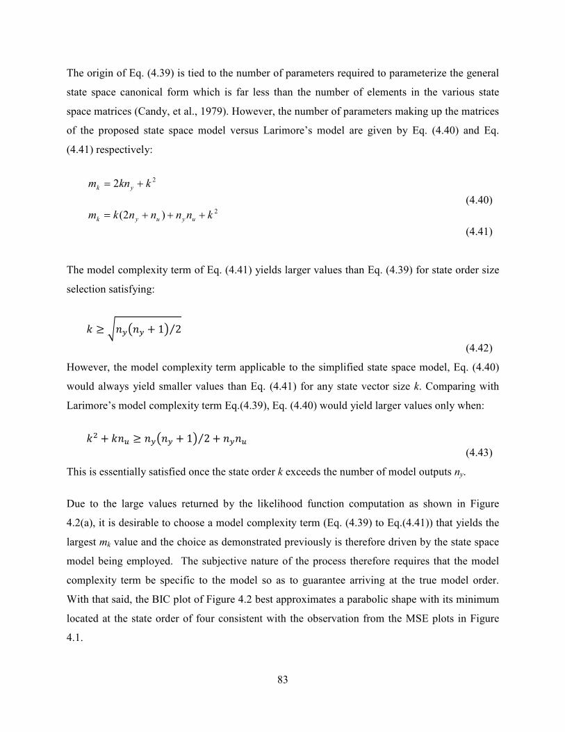
83

The origin of Eq. (4.39) is tied to the number of parameters required to parameterize the general

state space canonical form which is far less than the number of elements in the various state

space matrices (Candy, et al., 1979). However, the number of parameters making up the matrices

of the proposed state space model versus Larimore’s model are given by Eq. (4.40) and Eq.

(4.41) respectively:

22 kknm yk +=

(4.40) 2)2( knnnnkm uyuyk +++=

(4.41)

The model complexity term of Eq. (4.41) yields larger values than Eq. (4.39) for state order size

selection satisfying:

� ≥ 4\�f\� + 1h 23

(4.42)

However, the model complexity term applicable to the simplified state space model, Eq. (4.40)

would always yield smaller values than Eq. (4.41) for any state vector size k. Comparing with

Larimore’s model complexity term Eq.(4.39), Eq. (4.40) would yield larger values only when:

�? + �\î ≥ \�f\� + 1h 23 + \�\î

(4.43)

This is essentially satisfied once the state order k exceeds the number of model outputs ny.

Due to the large values returned by the likelihood function computation as shown in Figure

4.2(a), it is desirable to choose a model complexity term (Eq. (4.39) to Eq.(4.41)) that yields the

largest mk value and the choice as demonstrated previously is therefore driven by the state space

model being employed. The subjective nature of the process therefore requires that the model

complexity term be specific to the model so as to guarantee arriving at the true model order.

With that said, the BIC plot of Figure 4.2 best approximates a parabolic shape with its minimum

located at the state order of four consistent with the observation from the MSE plots in Figure

4.1.

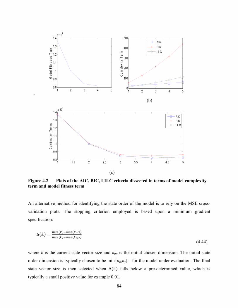
84

.

Figure 4.2 Plots of the AIC, BIC, LILC criteria dissected in terms of model complexity

term and model fitness term

An alternative method for identifying the state order of the model is to rely on the MSE cross-

validation plots. The stopping criterion employed is based upon a minimum gradient

specification:

∆� = @Ë7^ �@Ë7^�1 @Ë7^ �@Ë7^678

(4.44)

where k is the current state vector size and kint is the initial chosen dimension. The initial state

order dimension is typically chosen to be min{nu,ny} for the model under evaluation. The final

state vector size is then selected when Δk falls below a pre-determined value, which is

typically a small positive value for example 0.01.

4

1 2 3 4 50.8

0.9

1

1.1

1.2

1.3

1.4x 10

4

Model Fitnesss Term

1 2 3 4 50

100

200

300

400

500

Complexity Term

AIC

BIC

LILC

1 1.5 2 2.5 3 3.5 4 4.5 50.8

0.9

1

1.1

1.2

1.3

1.4x 10

4

Combination Terms

AIC

BIC

LILC

(b)

(c)

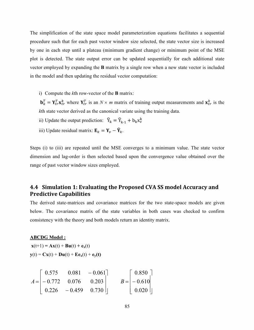
85

The simplification of the state space model parameterization equations facilitates a sequential

procedure such that for each past vector window size selected, the state vector size is increased

by one in each step until a plateau (minimum gradient change) or minimum point of the MSE

plot is detected. The state output error can be updated sequentially for each additional state

vector employed by expanding the B matrix by a single row when a new state vector is included

in the model and then updating the residual vector computation:

i) Compute the kth row-vector of the B matrix:

:� = O�I� p�I where O�I� is an N × m matrix of training output measurements and p�I is the

kth state vector derived as the canonical variate using the training data.

ii) Update the output prediction: )Yw� = Yw�-1 + b�x=�

iii) Update residual matrix: N^ = O> − Ow^.

Steps (i) to (iii) are repeated until the MSE converges to a minimum value. The state vector

dimension and lag-order is then selected based upon the convergence value obtained over the

range of past vector window sizes employed.

4.4 Simulation 1: Evaluating the Proposed CVA SS model Accuracy and

Predictive Capabilities

The derived state-matrices and covariance matrices for the two state-space models are given

below. The covariance matrix of the state variables in both cases was checked to confirm

consistency with the theory and both models return an identity matrix.

ABCDG Model :

x(t+1) = Ax(t) + Bu(t) + ex(t)

y(t) = Cx(t) + Du(t) + Eex(t) + ey(t)

−

−

−

=

730.0459.0226.0

203.0076.0772.0

061.0081.0575.0

A

−=

020.0

610.0

850.0

B

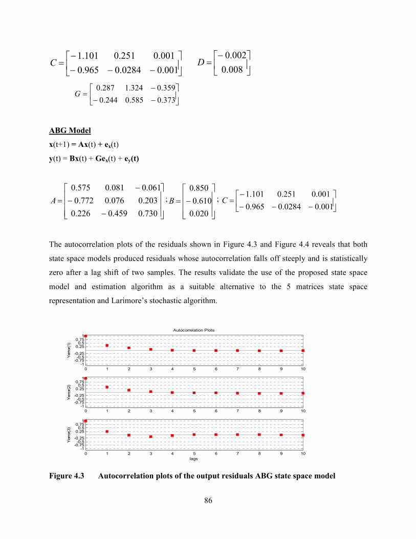
86

−−−

−=

001.00284.0965.0

001.0251.0101.1C

−−

−=

373.0585.0244.0

359.0324.1287.0G

ABG Model

x(t+1) = Ax(t) + ex(t)

y(t) = Bx(t) + Gex(t) + ey(t)

−

−

−

=

730.0459.0226.0

203.0076.0772.0

061.0081.0575.0

A ;

−=

020.0

610.0

850.0

B ;

−−−

−=

001.00284.0965.0

001.0251.0101.1C

The autocorrelation plots of the residuals shown in Figure 4.3 and Figure 4.4 reveals that both

state space models produced residuals whose autocorrelation falls off steeply and is statistically

zero after a lag shift of two samples. The results validate the use of the proposed state space

model and estimation algorithm as a suitable alternative to the 5 matrices state space

representation and Larimore’s stochastic algorithm.

Figure 4.3 Autocorrelation plots of the output residuals ABG state space model

−=

008.0

002.0D

0 1 2 3 4 5 6 7 8 9 10

-1-0.75-0.5-0.25

0.250.50.751

Autocorrelation Plots

Yerror(1)

0 1 2 3 4 5 6 7 8 9 10

-1-0.75-0.5-0.25

0.250.50.751

Yerror(2)

0 1 2 3 4 5 6 7 8 9 10

-1-0.75-0.5-0.25

0.250.50.751

Yerror(3)

lags

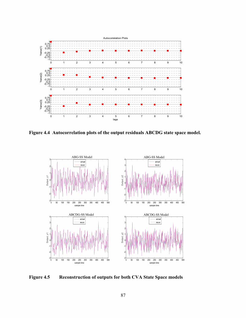
87

Figure 4.4 Autocorrelation plots of the output residuals ABCDG state space model.

Figure 4.5 Reconstruction of outputs for both CVA State Space models

0 1 2 3 4 5 6 7 8 9 10

-1-0.75-0.5-0.25

0.250.50.751

Autocorrelation PlotsYerror(1)

0 1 2 3 4 5 6 7 8 9 10

-1-0.75-0.5-0.25

0.250.50.751

Yerror(2)

0 1 2 3 4 5 6 7 8 9 10

-1-0.75-0.5-0.25

0.250.50.751

Yerror(3)

lags

0 50 100 150 200 250 300 350 400 450 500-3

-2

-1

0

1

2

3

Output, y1

sample time

ABC-SS model

0 50 100 150 200 250 300 350 400 450 500-3

-2

-1

0

1

2

3

4

Output, y2

sample time

ABC-SS model

0 50 100 150 200 250 300 350 400 450 500-3

-2

-1

0

1

2

3

4

Output, y1

sample time

ABCDE-SS model

0 50 100 150 200 250 300 350 400 450 500-3

-2

-1

0

1

2

3

4

Output, y2

sample time

ABCDE-SS model

actual

recon

actual

recon

actual

recon

actual

recon

ABG-SS Model ABG-SS Model

ABCDG-SS Model ABCDG-SS Model

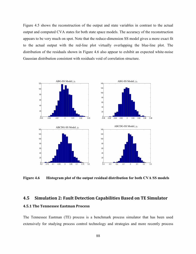
88

Figure 4.5 shows the reconstruction of the output and state variables in contrast to the actual

output and computed CVA states for both state space models. The accuracy of the reconstruction

appears to be very much on spot. Note that the reduce-dimension SS model gives a more exact fit

to the actual output with the red-line plot virtually overlapping the blue-line plot. The

distribution of the residuals shown in Figure 4.6 also appear to exhibit an expected white-noise

Gaussian distribution consistent with residuals void of correlation structure.

Figure 4.6 Histogram plot of the output residual distribution for both CVA SS models

4.5 Simulation 2: Fault Detection Capabilities Based on TE Simulator

4.5.1 The Tennessee Eastman Process

The Tennessee Eastman (TE) process is a benchmark process simulator that has been used

extensively for studying process control technology and strategies and more recently process

-0.03 -0.02 -0.01 0 0.01 0.02 0.030

20

40

60

80

100

120ABC-SS model, Output Y1

-0.08 -0.06 -0.04 -0.02 0 0.02 0.04 0.06 0.080

20

40

60

80

100

120

140ABC-SS model, Output Y2

-0.2 -0.15 -0.1 -0.05 0 0.05 0.1 0.15 0.20

20

40

60

80

100

120

140ABCDE-SS model, Output Y1

-0.4 -0.3 -0.2 -0.1 0 0.1 0.2 0.30

20

40

60

80

100

120

140ABCDE-SS model, Output Y2ABCDG-SS Model, y1

ABCDG-SS Model, y2

ABG-SS Model, y1 ABG-SS Model, y2

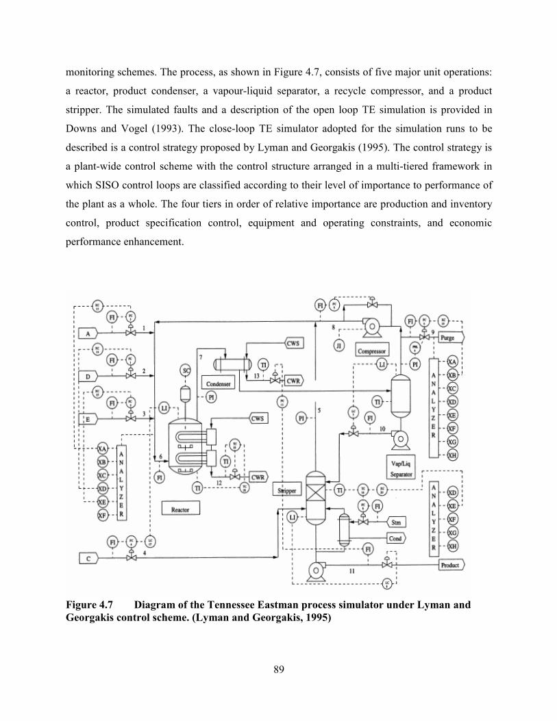
89

monitoring schemes. The process, as shown in Figure 4.7, consists of five major unit operations:

a reactor, product condenser, a vapour-liquid separator, a recycle compressor, and a product

stripper. The simulated faults and a description of the open loop TE simulation is provided in

Downs and Vogel (1993). The close-loop TE simulator adopted for the simulation runs to be

described is a control strategy proposed by Lyman and Georgakis (1995). The control strategy is

a plant-wide control scheme with the control structure arranged in a multi-tiered framework in

which SISO control loops are classified according to their level of importance to performance of

the plant as a whole. The four tiers in order of relative importance are production and inventory

control, product specification control, equipment and operating constraints, and economic

performance enhancement.

Figure 4.7 Diagram of the Tennessee Eastman process simulator under Lyman and

Georgakis control scheme. (Lyman and Georgakis, 1995)

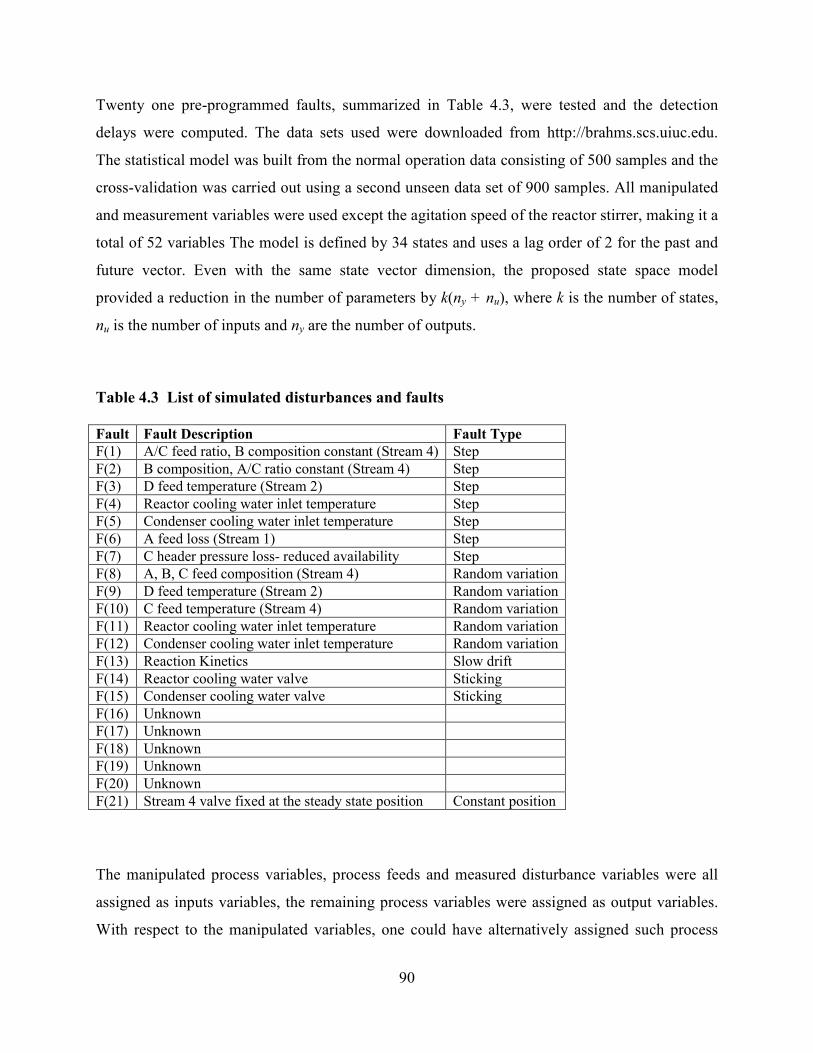
90

Twenty one pre-programmed faults, summarized in Table 4.3, were tested and the detection

delays were computed. The data sets used were downloaded from http://brahms.scs.uiuc.edu.

The statistical model was built from the normal operation data consisting of 500 samples and the

cross-validation was carried out using a second unseen data set of 900 samples. All manipulated

and measurement variables were used except the agitation speed of the reactor stirrer, making it a

total of 52 variables The model is defined by 34 states and uses a lag order of 2 for the past and

future vector. Even with the same state vector dimension, the proposed state space model

provided a reduction in the number of parameters by k(ny + nu), where k is the number of states,

nu is the number of inputs and ny are the number of outputs.

Table 4.3 List of simulated disturbances and faults

Fault Fault Description Fault Type

F(1) A/C feed ratio, B composition constant (Stream 4) Step

F(2) B composition, A/C ratio constant (Stream 4) Step

F(3) D feed temperature (Stream 2) Step

F(4) Reactor cooling water inlet temperature Step

F(5) Condenser cooling water inlet temperature Step

F(6) A feed loss (Stream 1) Step

F(7) C header pressure loss- reduced availability Step

F(8) A, B, C feed composition (Stream 4) Random variation

F(9) D feed temperature (Stream 2) Random variation

F(10) C feed temperature (Stream 4) Random variation

F(11) Reactor cooling water inlet temperature Random variation

F(12) Condenser cooling water inlet temperature Random variation

F(13) Reaction Kinetics Slow drift

F(14) Reactor cooling water valve Sticking

F(15) Condenser cooling water valve Sticking

F(16) Unknown

F(17) Unknown

F(18) Unknown

F(19) Unknown

F(20) Unknown

F(21) Stream 4 valve fixed at the steady state position Constant position

The manipulated process variables, process feeds and measured disturbance variables were all

assigned as inputs variables, the remaining process variables were assigned as output variables.

With respect to the manipulated variables, one could have alternatively assigned such process

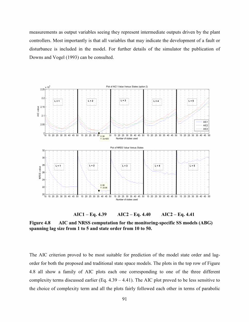
91

measurements as output variables seeing they represent intermediate outputs driven by the plant

controllers. Most importantly is that all variables that may indicate the development of a fault or

disturbance is included in the model. For further details of the simulator the publication of

Downs and Vogel (1993) can be consulted.

AIC1 – Eq. 4.39 AIC2 – Eq. 4.40 AIC2 – Eq. 4.41

Figure 4.8 AIC and NRSS computation for the monitoring-specific SS models (ABG)

spanning lag size from 1 to 5 and state order from 10 to 50.

The AIC criterion proved to be most suitable for prediction of the model state order and lag-

order for both the proposed and traditional state space models. The plots in the top row of Figure

4.8 all show a family of AIC plots each one corresponding to one of the three different

complexity terms discussed earlier (Eq. 4.39 – 4.41). The AIC plot proved to be less sensitive to

the choice of complexity term and all the plots fairly followed each other in terms of parabolic

10 15 20 25 30 35 40 45 50 15 20 25 30 35 40 45 50 15 20 25 30 35 40 45 50 15 20 25 30 35 40 45 50 15 20 25 30 35 40 45 502

2.05

2.1

2.15

2.2

2.25x 10

5

Plot of AIC1 Value Versus States (option 2)

AIC value

Number of states usedX: 68

Y: 2e+005

10 15 20 25 30 35 40 45 50 15 20 25 30 35 40 45 50 15 20 25 30 35 40 45 50 15 20 25 30 35 40 45 50 15 20 25 30 35 40 45 5020

22

24

26

28

30

32Plot of NRSS Value Versus States

NRSS value

Number of states used

X: 68

Y: 20.98

AIC1

AIC2

AIC3

L = 1 L = 2 L = 3 L = 4 L = 5

L = 5L = 4L = 3L = 2L = 1

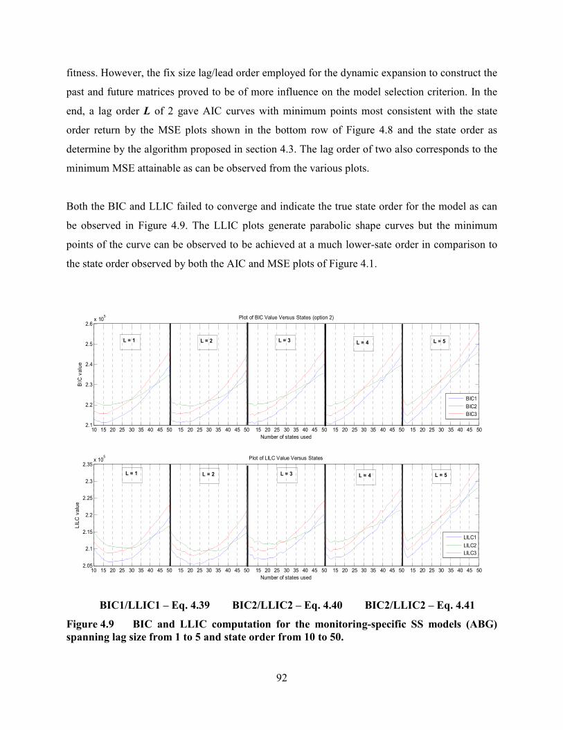
92

fitness. However, the fix size lag/lead order employed for the dynamic expansion to construct the

past and future matrices proved to be of more influence on the model selection criterion. In the

end, a lag order L of 2 gave AIC curves with minimum points most consistent with the state

order return by the MSE plots shown in the bottom row of Figure 4.8 and the state order as

determine by the algorithm proposed in section 4.3. The lag order of two also corresponds to the

minimum MSE attainable as can be observed from the various plots.

Both the BIC and LLIC failed to converge and indicate the true state order for the model as can

be observed in Figure 4.9. The LLIC plots generate parabolic shape curves but the minimum

points of the curve can be observed to be achieved at a much lower-sate order in comparison to

the state order observed by both the AIC and MSE plots of Figure 4.1.

BIC1/LLIC1 – Eq. 4.39 BIC2/LLIC2 – Eq. 4.40 BIC2/LLIC2 – Eq. 4.41

Figure 4.9 BIC and LLIC computation for the monitoring-specific SS models (ABG)

spanning lag size from 1 to 5 and state order from 10 to 50.

10 15 20 25 30 35 40 45 50 15 20 25 30 35 40 45 50 15 20 25 30 35 40 45 50 15 20 25 30 35 40 45 50 15 20 25 30 35 40 45 502.05

2.1

2.15

2.2

2.25

2.3

2.35x 10

5 Plot of LILC Value Versus States

LILC value


10 15 20 25 30 35 40 45 50 15 20 25 30 35 40 45 50 15 20 25 30 35 40 45 50 15 20 25 30 35 40 45 50 15 20 25 30 35 40 45 502.1

2.2

2.3

2.4

2.5

2.6x 10

5 Plot of BIC Value Versus States (option 2)

BIC value


BIC1

BIC2

BIC3

LILC1

LILC2

LILC3

L = 1L = 4

L = 3L = 2 L = 5

L = 5L = 2 L = 3 L = 4L = 1

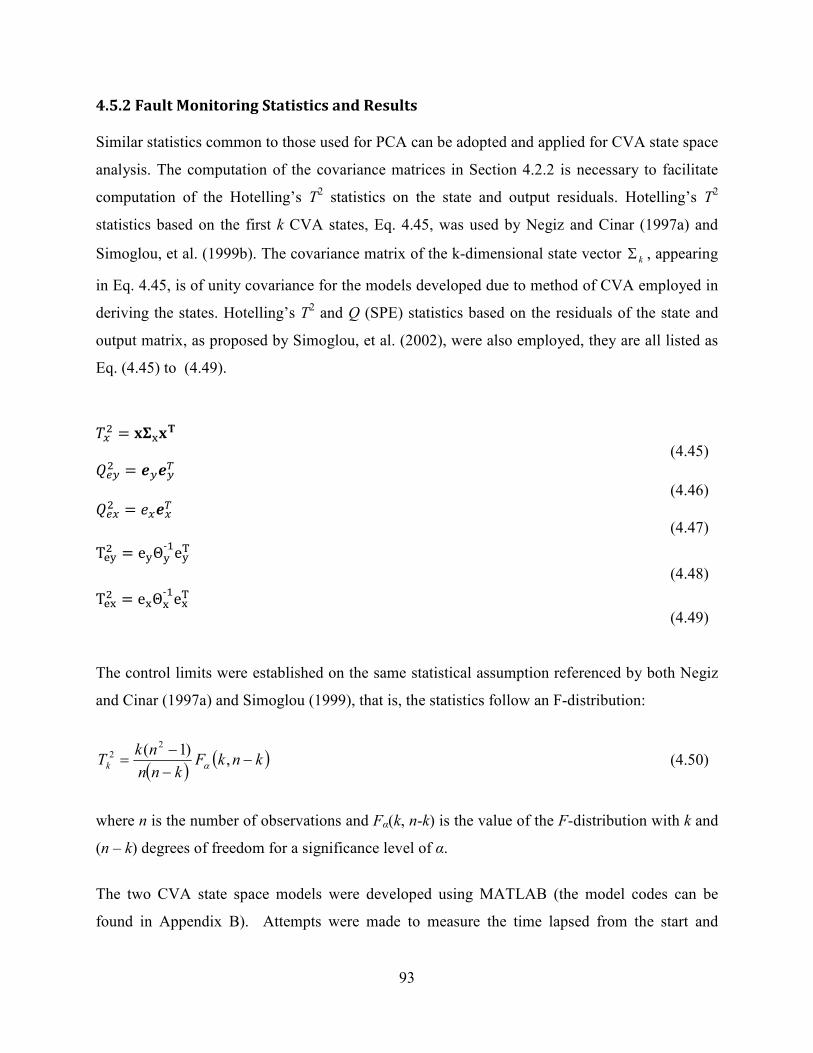
93

4.5.2 Fault Monitoring Statistics and Results

Similar statistics common to those used for PCA can be adopted and applied for CVA state space

analysis. The computation of the covariance matrices in Section 4.2.2 is necessary to facilitate

computation of the Hotelling’s T2 statistics on the state and output residuals. Hotelling’s T

2

statistics based on the first k CVA states, Eq. 4.45, was used by Negiz and Cinar (1997a) and

Simoglou, et al. (1999b). The covariance matrix of the k-dimensional state vector kΣ , appearing

in Eq. 4.45, is of unity covariance for the models developed due to method of CVA employed in

deriving the states. Hotelling’s T2 and Q (SPE) statistics based on the residuals of the state and

output matrix, as proposed by Simoglou, et al. (2002), were also employed, they are all listed as

Eq. (4.45) to (4.49).

r�? = p��p� (4.45) y7�? = q�q��

(4.46) y7�? = ?�q��

(4.47)

Tt�? = e�Θ�-1e��

(4.48)

Tt�? = e�Θ�-1e��

(4.49)

The control limits were established on the same statistical assumption referenced by both Negiz

and Cinar (1997a) and Simoglou (1999), that is, the statistics follow an F-distribution:

( )( )knkF

knn

nkTk −

−−

= ,)1( 2

2

α (4.50)

where n is the number of observations and Fα(k, n-k) is the value of the F-distribution with k and

(n – k) degrees of freedom for a significance level of α.

The two CVA state space models were developed using MATLAB (the model codes can be

found in Appendix B). Attempts were made to measure the time lapsed from the start and

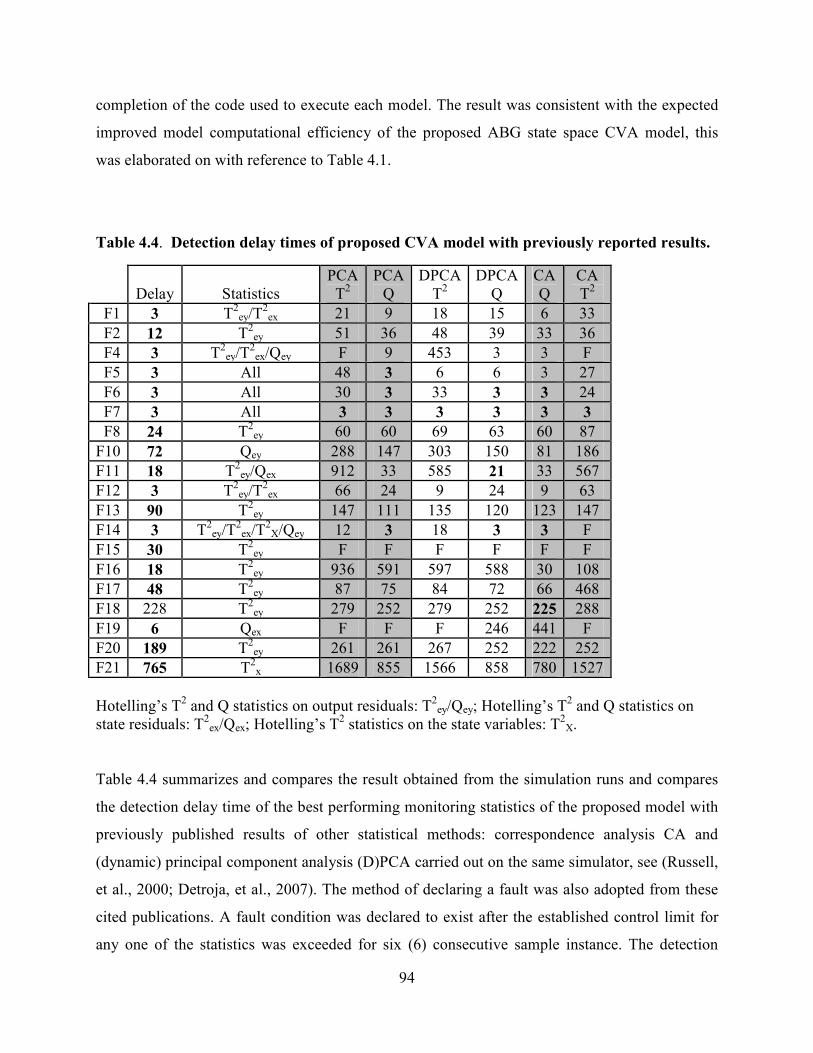
94

completion of the code used to execute each model. The result was consistent with the expected

improved model computational efficiency of the proposed ABG state space CVA model, this

was elaborated on with reference to Table 4.1.

Table 4.4. Detection delay times of proposed CVA model with previously reported results.

Delay Statistics

PCA

T2

PCA

Q

DPCA

T2

DPCA

Q

CA

Q

CA

T2

F1 3 T2

ey/T2

ex 21 9 18 15 6 33

F2 12 T2

ey 51 36 48 39 33 36

F4 3 T2

ey/T2

ex/Qey F 9 453 3 3 F

F5 3 All 48 3 6 6 3 27

F6 3 All 30 3 33 3 3 24

F7 3 All 3 3 3 3 3 3

F8 24 T2

ey 60 60 69 63 60 87

F10 72 Qey 288 147 303 150 81 186

F11 18 T2

ey/Qex 912 33 585 21 33 567

F12 3 T2

ey/T2

ex 66 24 9 24 9 63

F13 90 T2

ey 147 111 135 120 123 147

F14 3 T2

ey/T2

ex/T2

X/Qey 12 3 18 3 3 F

F15 30 T2

ey F F F F F F

F16 18 T2

ey 936 591 597 588 30 108

F17 48 T2

ey 87 75 84 72 66 468

F18 228 T2

ey 279 252 279 252 225 288

F19 6 Qex F F F 246 441 F

F20 189 T2

ey 261 261 267 252 222 252

F21 765 T2

x 1689 855 1566 858 780 1527

Hotelling’s T2 and Q statistics on output residuals: T

2ey/Qey; Hotelling’s T

2 and Q statistics on

state residuals: T2

ex/Qex; Hotelling’s T2 statistics on the state variables: T

2X.

Table 4.4 summarizes and compares the result obtained from the simulation runs and compares

the detection delay time of the best performing monitoring statistics of the proposed model with

previously published results of other statistical methods: correspondence analysis CA and

(dynamic) principal component analysis (D)PCA carried out on the same simulator, see (Russell,

et al., 2000; Detroja, et al., 2007). The method of declaring a fault was also adopted from these

cited publications. A fault condition was declared to exist after the established control limit for

any one of the statistics was exceeded for six (6) consecutive sample instance. The detection

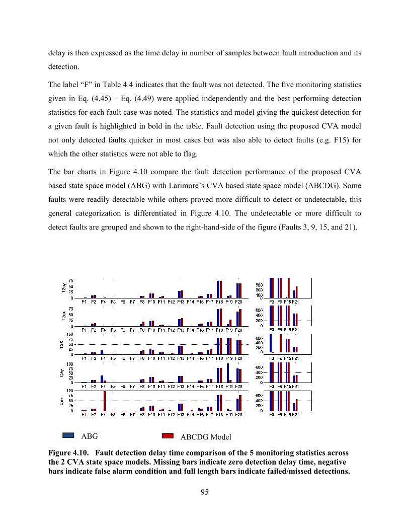
95

delay is then expressed as the time delay in number of samples between fault introduction and its

detection.

The label “F” in Table 4.4 indicates that the fault was not detected. The five monitoring statistics

given in Eq. (4.45) – Eq. (4.49) were applied independently and the best performing detection

statistics for each fault case was noted. The statistics and model giving the quickest detection for

a given fault is highlighted in bold in the table. Fault detection using the proposed CVA model

not only detected faults quicker in most cases but was also able to detect faults (e.g. F15) for

which the other statistics were not able to flag.

The bar charts in Figure 4.10 compare the fault detection performance of the proposed CVA

based state space model (ABG) with Larimore’s CVA based state space model (ABCDG). Some

faults were readily detectable while others proved more difficult to detect or undetectable, this

general categorization is differentiated in Figure 4.10. The undetectable or more difficult to

detect faults are grouped and shown to the right-hand-side of the figure (Faults 3, 9, 15, and 21).

Figure 4.10. Fault detection delay time comparison of the 5 monitoring statistics across

the 2 CVA state space models. Missing bars indicate zero detection delay time, negative

bars indicate false alarm condition and full length bars indicate failed/missed detections.

ABG

Model ABCDG Model

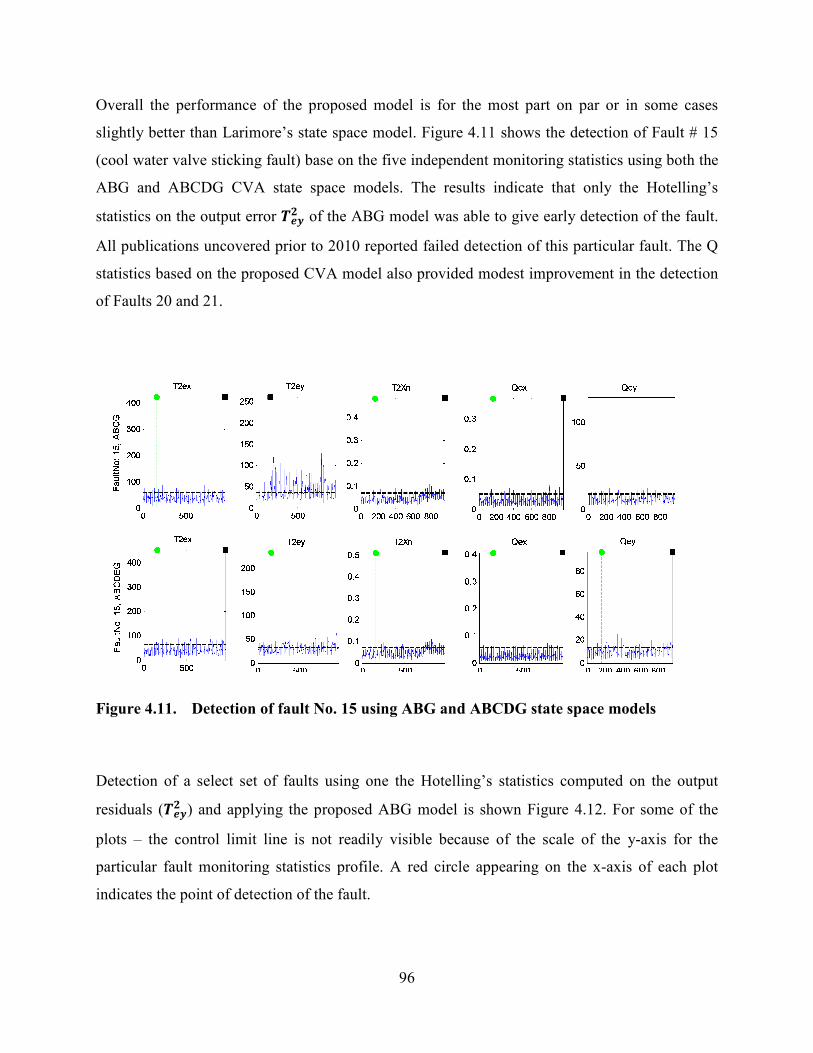
96

Overall the performance of the proposed model is for the most part on par or in some cases

slightly better than Larimore’s state space model. Figure 4.11 shows the detection of Fault # 15

(cool water valve sticking fault) base on the five independent monitoring statistics using both the

ABG and ABCDG CVA state space models. The results indicate that only the Hotelling’s

statistics on the output error oq¢" of the ABG model was able to give early detection of the fault.

All publications uncovered prior to 2010 reported failed detection of this particular fault. The Q

statistics based on the proposed CVA model also provided modest improvement in the detection

of Faults 20 and 21.

Figure 4.11. Detection of fault No. 15 using ABG and ABCDG state space models

Detection of a select set of faults using one the Hotelling’s statistics computed on the output

residuals (oq¢" ) and applying the proposed ABG model is shown Figure 4.12. For some of the

plots – the control limit line is not readily visible because of the scale of the y-axis for the

particular fault monitoring statistics profile. A red circle appearing on the x-axis of each plot

indicates the point of detection of the fault.

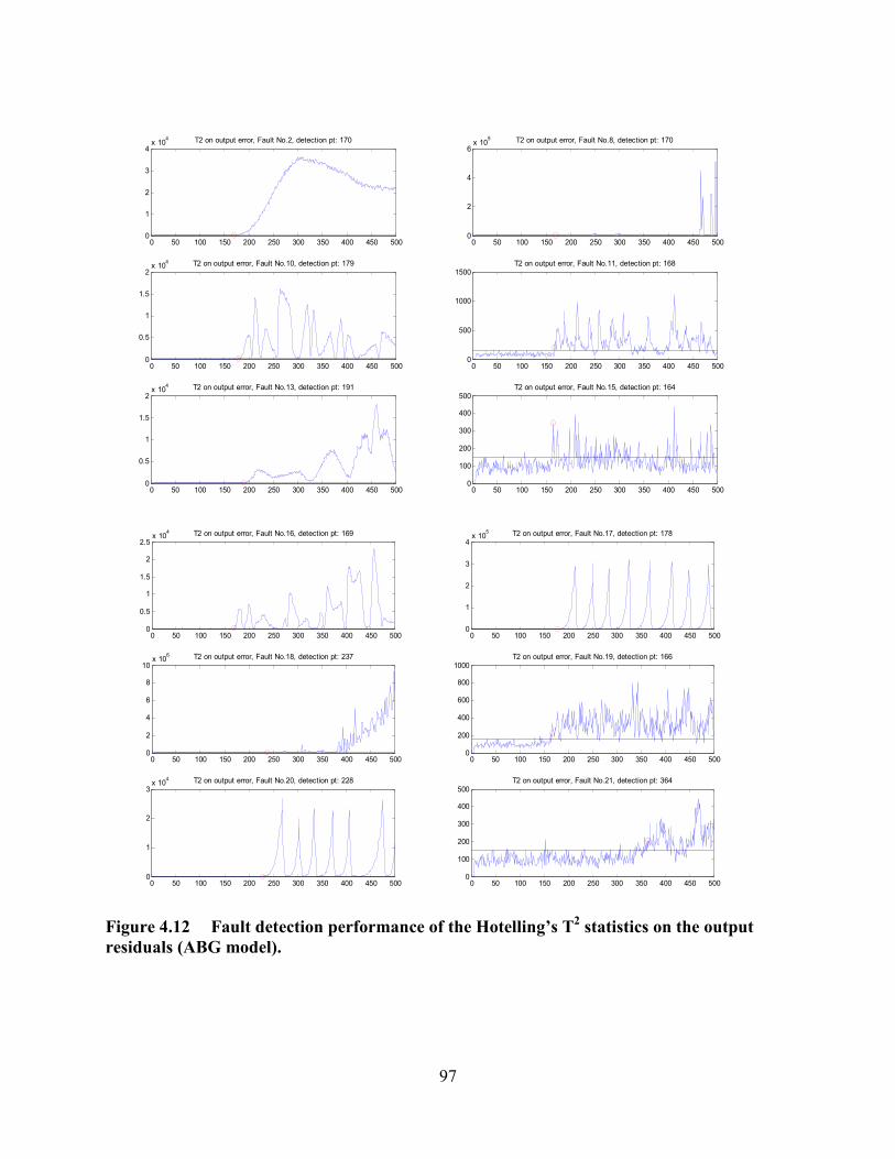
97

Figure 4.12 Fault detection performance of the Hotelling’s T2 statistics on the output

residuals (ABG model).

0 50 100 150 200 250 300 350 400 450 5000

1

2

3

4x 10

4 T2 on output error, Fault No.2, detection pt: 170

0 50 100 150 200 250 300 350 400 450 5000

2

4

6x 10


0 50 100 150 200 250 300 350 400 450 5000

0.5

1

1.5

2x 10


0 50 100 150 200 250 300 350 400 450 5000

500

1000

1500T2 on output error, Fault No.11, detection pt: 168

0 50 100 150 200 250 300 350 400 450 5000

0.5

1

1.5

2x 10


0 50 100 150 200 250 300 350 400 450 5000

100

200

300

400


0 50 100 150 200 250 300 350 400 450 5000

0.5

1

1.5

2

2.5x 10


0 50 100 150 200 250 300 350 400 450 5000

1

2

3

4x 10


0 50 100 150 200 250 300 350 400 450 5000

2

4

6

8

10x 10


0 50 100 150 200 250 300 350 400 450 5000

200

400

600

800


0 50 100 150 200 250 300 350 400 450 5000

1

2

3x 10


0 50 100 150 200 250 300 350 400 450 5000

100

200

300

400


98

A more recent publication by Odiowei and Cao (2010) also conducted a comparative analysis of

their proposed state space independent component analysis SSICA approach against the

performance of the CVA and dynamic independent component analysis DICA approach. The

SSICA is essentially a combination of a first stage CVA state space model and a second stage

independent component analysis ICA approach. The authors attributed the improved

performance of SSICA over the usual DICA approach due to the fact that CVA SS model is

better suited for capturing the dynamics of a process than a dynamic principal component

analysis DPCA method upon which DICA is based. ICA method is said to be better suited for

process characterised by non-Gaussian distribution.

Both detection delay times and percentage reliability metrics were analysed, Table 4.5 compares

extracts of their results with the fault monitoring performance of the proposed CVA state space

performance. The percentage reliability is defined as the percentage of the samples outside the

control limits. The proposed model outperformed or detected on par with the SSICA/DICA

method in terms of detection delay time for faults 1,2,4,5,6,7,11,12,13,14,16,17 and 19 but

performed inferior for the remaining faults not including fault 21 which was not included in

Odiowei and Cao (2010) fault simulation and analysis study.

In particular, Odiowei and Cao (2010) have reported successful detection of faults # 3 and # 9

with relatively high reliability. Based on the authors’ literature review, no other publications

have reported achieving such. Beside these two faults, the fault detection reliability was above

97% for all detectable faults for the proposed CVA state space model and therefore gave an

overall better fault performance than both the DICA and SSICA schemes in that regards.

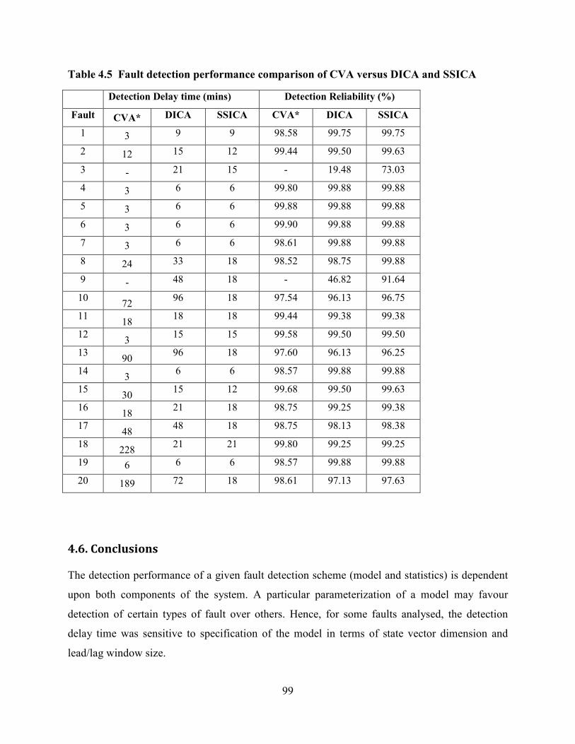
99

Table 4.5 Fault detection performance comparison of CVA versus DICA and SSICA

Detection Delay time (mins) Detection Reliability (%)

Fault CVA* DICA SSICA CVA* DICA SSICA

1 3 9 9 98.58 99.75 99.75

2 12 15 12 99.44 99.50 99.63

3 - 21 15 - 19.48 73.03

4 3 6 6 99.80 99.88 99.88

5 3 6 6 99.88 99.88 99.88

6 3 6 6 99.90 99.88 99.88

7 3 6 6 98.61 99.88 99.88

8 24 33 18 98.52 98.75 99.88

9 - 48 18 - 46.82 91.64

10 72

96 18 97.54 96.13 96.75

11 18

18 18 99.44 99.38 99.38

12 3

15 15 99.58 99.50 99.50

13 90

96 18 97.60 96.13 96.25

14 3

6 6 98.57 99.88 99.88

15 30

15 12 99.68 99.50 99.63

16 18

21 18 98.75 99.25 99.38

17 48

48 18 98.75 98.13 98.38

18 228

21 21 99.80 99.25 99.25

19 6 6 6 98.57 99.88 99.88

20 189 72 18 98.61 97.13 97.63

4.6. Conclusions

The detection performance of a given fault detection scheme (model and statistics) is dependent

upon both components of the system. A particular parameterization of a model may favour

detection of certain types of fault over others. Hence, for some faults analysed, the detection

delay time was sensitive to specification of the model in terms of state vector dimension and

lead/lag window size.

100

A simplified CVA based state-space model design for the specific purpose of process monitoring

was achieved using a simpler and more efficiently estimation of a reduced set of state space

parameter matrices. The performance integrity of the state space model was maintained in

conjunction with a dramatic reduction in the number of model parameters and simplification of

the set of stochastic estimation equations used to derive the model parameters. Application

results on the Tennessee Eastman benchmark process indicate that the proposed state space

representation and model development technique provides comparable, and in many cases better,

fault detection performance than the traditional CVA state space modelling technique. Most

notable is the detection of fault No. 15 in the Tennessee Eastman benchmark process and the

significant reduction in detection delay time achieved for the more difficult to detect faults. The

overall best performing monitoring statistics in terms of fault detection and detection delay time

is the Hotelling’s T2 statistics of the output residuals T

2ey.

The fault detection performance also faired comparably to that reported for the DICA and SSICA

schemes (Odiowei and Cao 2010) save for the unprecedented detection of faults # 3 and 9.

However, for those faults detectable by the proposed CVA method, the percentage performance

reliability was better on average than that of DICA and SSICA. Future research could explore

what further fault performance improvements could be yield from combining the ICA approach

with a CVA state space model as proposed in this paper.

101

Chapter 5 : Hybrid Model Based Approach to Process-

Monitoring

5.1 Introduction

Previous researchers have proposed several different hybrid framework for process

monitoring and modeling. Some methods have included hybrid approaches involving

integration of different data driven modeling techniques, Yan (2010). Other approaches have

considered combining linear or nonlinear data driven model based approaches with

mechanistic model based approaches when there exist information about known kinetics,

material balance equations, and other first principle or heuristic knowledge of the system

being modeled or monitored (Lee, et al., 2005; Oliveira, 2004; Peres, et al., 2001; Psichogios

and Ungar, 1992).

As it relates to the specific application of process performance monitoring and fault

detection, Wachs and Lewin (1998) proposed model-based PCA and more recently

McPherson et al (2002) proposed a super-model base approach to monitoring of batch

processes. The main difference or improvement of super model-based PCA over model-base

PCA proposed by Wachs and Lewin (1998) is that the hybrid model incorporated the use of

an additional stage referred to as an error model. The error model was used to augment the

102

mechanistic plant model to remove whatever remaining structure that may exist in its

residuals, that is, the plant-mechanistic model residuals.

This chapter contributes to research and exploration into the suitability and advantages that a

hybrid model architecture may offer to fault detection and process monitoring applications.

Specific improvements and implementation considerations are given to the hybrid

mechanistic-data driven model based monitoring scheme applicable to close-loop process

operations. The impact of model-plant mismatches on the fault detection and monitoring

performance is also considered. The work presented in this chapter demonstrates the

feasibility of combining a statistical data based model with a mechanistic model

implementation that does not require implementation of the plant control loops to perform

fault detection.

The effectiveness of the hybrid mechanistic-data driven fault monitoring scheme and the

problems arising from plant model mismatch when employing mechanistic first principle

models are both analyzed using a simulated CSTR process with a recycle via a heat

exchanger. The results provide evidence that both the prediction and fault detection

performance of the mechanistic model can be enhanced by compensating the mechanistic or

first principle model with a data-driven based statistical model. Linear PLS data-based

modeling and a non-linear PLS implementation based on a quadratic PLS (QPLS)

implementation originally proposed by Wold et. al (1989) were employed. Both data-based

models proved to offer effective compensation for the mechanistic models implemented and

the associated plant-model mismatch. The most suitable model for fault detection was

identified from fault detection simulation analysis results.

An alternative hybrid scheme combining two different types of statistical data driven models

was also explored. The hybrid architecture combines a neural network model with an

ordinary least squares (OLS) regression model to map the nonlinear plant dynamics of a

simulated distillation column developed using ChemCad version 6.

103

The remainder of the chapter is organized as follows. Section 5.2 provides an overview of the

first principle equations applied in the development of the simulated CSTR. The subsection also

explains the method used to introduce and evaluate the plant-model mismatch issue. In section

5.3 several hybrid modelling schemes are proposed and evaluated to assess what improvement

the hybrid approaches bring to bear on the residual whitening and model predictive capabilities.

In section 5.4 a subset of the hybrid models presented in section 5.3 is further analyzed and

combined with Hotelling’s T2 and Q statistics to evaluate their fault detection performance.

Section 5.5 documents an alternative hybrid data driven model scheme which combines two

different classes of statistical data modelling approaches. The hybrid scheme was evaluated and

applied to performance monitoring of a simulated distillation column.

5.2 The Plant, Model, and Fault Simulator

5.2.1 CSTR Plant Simulator

The CSTR system shown in Figure 5.1 is an adaptation of a similar model used by Zhang et al

(1996) to evaluate the detection and diagnostic capable of principal component analysis PCA

based monitoring scheme. The reaction model is one of an irreversible heterogeneous catalytic

exothermic conversion of a reactant A to a product B. The control objective is to maintain the

product concentration at a desired level by indirect control of the temperature, residence time and

mixing conditions in the CSTR. A recycle product stream circulated via a heat exchanger (HTX)

is used to facilitate the temperature control and ensure well-mixed condition. The reactor

temperature is controlled by manipulating the flow rate of the cold water feed to the heat

exchanger via a cascade control loop. The residence time is controlled by maintaining the level

in the reactor.

104

Figure 5.1. Continuous Stirred Tank Reactor CSTR with recycle loop via Heat

Exchanger HTX.

The reaction and dynamics of the reactor was modelled using Eq.(5.1) through to Eq(5.6).

The rate of change of the liquid level H in the reactor is given by:

<A<� = 1B 31 + 3? − 3�

(5.1)

where F1 is the flow rate of the inlet stream, F2 is the flow rate of the recycle stream and F3 is the

flow rate of the stream exiting in the reactor.

The rate of change of the reactant concentration Cr in the reactor is given by:

<CD<� = ïCDEBA + CD

BA 3? − 3� − [I?�FD/�ýI

(5.2)

From the mass-balance applied around the reactor F2 – F3 = -F1 therefore Eq. (5.2) maybe

written as:

F1

F2

F3

F4

Fc

105

<CD<� = ïBA ýIÚ − ýI − [I?�FD/�ýI

The rate of change of the product concentration Cp in the outlet stream F4 is net of that being

converted (generated) in the reactor, that which already exist in the tank outlet stream F3 and the

amount being taken away by the recycle stream F2:

<CG<� = [I?�FD/�ýI + CGBA 3� − 3?

(5.3)

Again applying the mass balance equation Eq.(5.3) may alternatively be expressed as:

<CG<� = [I?�FD/�ýI + ïBA ýB

The rate of change of the temperature in the reactor is given by:

HIü? <�D<� = ü131r1 − rI − ü?3?rI − r? + II[I?�FD/�ýI

(5.4)

where T1 is the temperature of stream F1, T2 is the temperature of stream F2, and Tr is the

temperature of the reactor.

The dynamics of the heat exchanger was modeled by the non-linear first order equation given by:

ü?� <�J<� = ü?3?rI − r? − � KïLMïL�Ú.NKïLM� OPQP3Pr? − rP

(5.5)

where ü1 = OIQIýIÚ + 1 − ýIÚ OËQË and ü? = OIQIfýI + ýBh + f1 − ýI − ýBhOËQË.

The pressure at the base of the tank is given by:

4Ú = IOIfýI + ýBh + f1 − ýI − ýBhOË

(5.6)

The description of all the constants and variables for the model along with their assign values

and steady state condition is provided in Table 5.1.

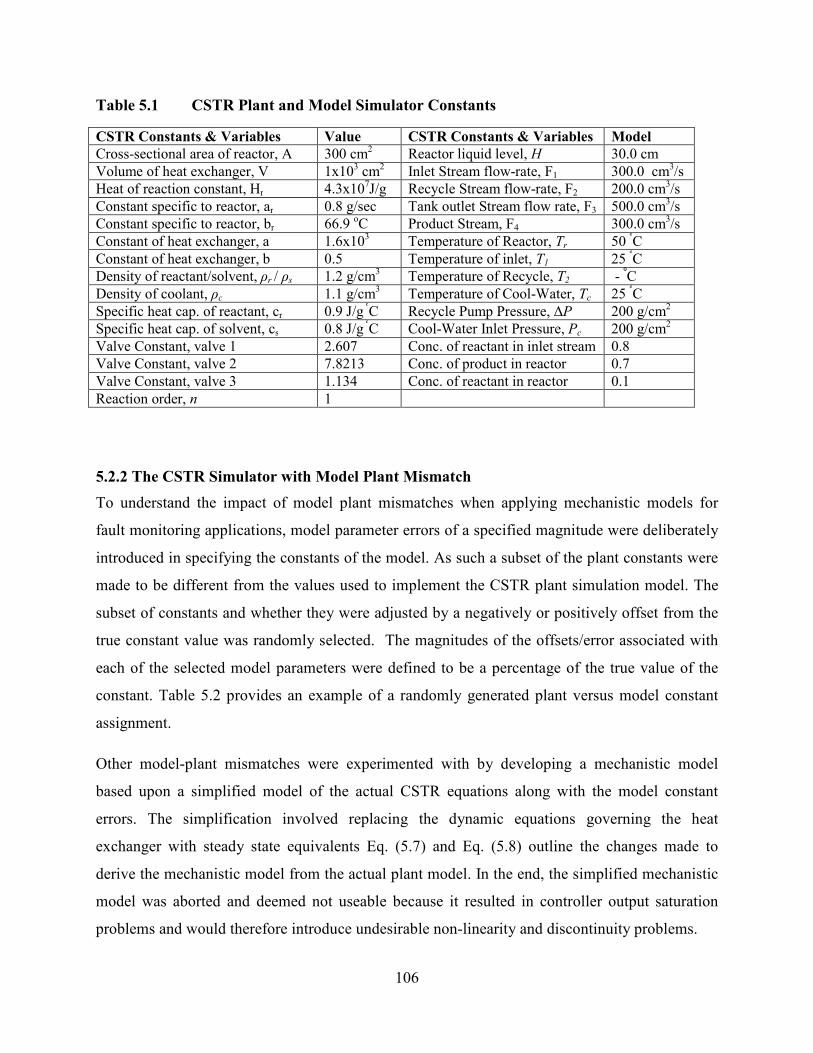
106

Table 5.1 CSTR Plant and Model Simulator Constants

CSTR Constants & Variables Value CSTR Constants & Variables Model

Cross-sectional area of reactor, A 300 cm2

Reactor liquid level, H 30.0 cm

Volume of heat exchanger, V 1x103 cm

2 Inlet Stream flow-rate, F1 300.0 cm

3/s

Heat of reaction constant, Hr 4.3x107J/g Recycle Stream flow-rate, F2 200.0 cm

3/s

Constant specific to reactor, ar 0.8 g/sec Tank outlet Stream flow rate, F3 500.0 cm3/s

Constant specific to reactor, br 66.9 ᴏC Product Stream, F4 300.0 cm

3/s

Constant of heat exchanger, a 1.6x103 Temperature of Reactor, Tr 50

ºC

Constant of heat exchanger, b 0.5 Temperature of inlet, T1 25 ºC

Density of reactant/solvent, ρr / ρs 1.2 g/cm3

Temperature of Recycle, T2 - ºC

Density of coolant, ρc 1.1 g/cm3 Temperature of Cool-Water, Tc 25

ºC

Specific heat cap. of reactant, cr 0.9 J/g ºC Recycle Pump Pressure, ∆P 200 g/cm

2

Specific heat cap. of solvent, cs 0.8 J/g ºC Cool-Water Inlet Pressure, Pc 200 g/cm

2

Valve Constant, valve 1 2.607 Conc. of reactant in inlet stream 0.8

Valve Constant, valve 2 7.8213 Conc. of product in reactor 0.7

Valve Constant, valve 3 1.134 Conc. of reactant in reactor 0.1

Reaction order, n 1

5.2.2 The CSTR Simulator with Model Plant Mismatch

To understand the impact of model plant mismatches when applying mechanistic models for

fault monitoring applications, model parameter errors of a specified magnitude were deliberately

introduced in specifying the constants of the model. As such a subset of the plant constants were

made to be different from the values used to implement the CSTR plant simulation model. The

subset of constants and whether they were adjusted by a negatively or positively offset from the

true constant value was randomly selected. The magnitudes of the offsets/error associated with

each of the selected model parameters were defined to be a percentage of the true value of the

constant. Table 5.2 provides an example of a randomly generated plant versus model constant

assignment.

Other model-plant mismatches were experimented with by developing a mechanistic model

based upon a simplified model of the actual CSTR equations along with the model constant

errors. The simplification involved replacing the dynamic equations governing the heat

exchanger with steady state equivalents Eq. (5.7) and Eq. (5.8) outline the changes made to

derive the mechanistic model from the actual plant model. In the end, the simplified mechanistic

model was aborted and deemed not useable because it resulted in controller output saturation

problems and would therefore introduce undesirable non-linearity and discontinuity problems.

107

The steady state equation for the heat exchanger is derived from Eq. (5.5) by setting the rate of

change of the recycle loop temperature term to zero:

r? = RJïJ�D�õ STLMTLUE.VSTLMöWLPLïL�Lõ STLM

TLUE.VSTLMöWLPLïL�RJïJ (5.7)

For the case where the constant are given the assignments a = 2 and b = 1 the above reduces to:

r? = RJïJ�D�WLPLïL�LWLPLïL�RJïJ (5.8)

Table 5.2 Model Mismatch Case: Plant vs Model Constants Employed

CSTR Model Constants Plant Model

Cross-sectional area of reactor, A 300 cm2

300 cm2

Volume of heat exchanger, V 1x103 cm

2 1x10

3 cm

2

Heat of reaction constant, Hr 4.3x107J/g 4.68x10

7J/g

Constant specific to reactor, ar 0.8 g/sec 0.75 g/sec

Constant specific to reactor, br 66.9 ᴏC 68.2 ᴏ

C

Constant of heat exchanger, a 1.6x103 1.68x10

3

Constant of heat exchanger, b 0.5 0.55

Density of reactant/product 1.2 g/cm3

1.31 g/cm3

Density of coolant 1.1 g/cm3 1.08 g/cm

3

Specific heat cap. of reactant, cr 0.9 J/g ᴏC 0.913 J/g

ᴏC

Specific heat cap. of product 0.8 J/g ᴏC 0.787 J/g

ᴏC

Valve Constant, valve 1 2.607 2.744



Reaction order 1 1.044

Figure 5.2 illustrates the impact of the model plant mismatch for a subset of the process variables

generated by the model. The deviation/offset of the model outputs from those of the actual plant

is shown to increase with increasing percentages of model-mismatches. Note, however, that the

difference in the plant-model outputs is bounded for the entire simulation run time for all cases

of model-plant mismatch presented. This is a necessary condition for any model to be used for

fault detection applications.

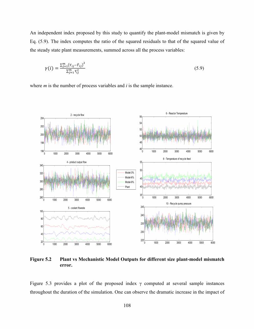
108

An independent index proposed by this study to quantify the plant-model mismatch is given by

Eq. (5.9). The index computes the ratio of the squared residuals to that of the squared value of

the steady state plant measurements, summed across all the process variables:

XÓ = Y fZ6��Z¼6�hJ[�\Y Z6�J[�\

(5.9)

where m is the number of process variables and i is the sample instance.

Figure 5.2 Plant vs Mechanistic Model Outputs for different size plant-model mismatch

error.

Figure 5.3 provides a plot of the proposed index γ computed at several sample instances

throughout the duration of the simulation. One can observe the dramatic increase in the impact of

0 1000 2000 3000 4000 5000 6000196

198

200

202

2042 - recycle flow

0 1000 2000 3000 4000 5000 6000260

280

300

320

3404 - product output flow

0 1000 2000 3000 4000 5000 600020

40

60

80

1005 - coolant flowrate

0 1000 2000 3000 4000 5000 600046

48

50

52

54

566 - Reactor Temperature

0 1000 2000 3000 4000 5000 600035

40

45

50

558 - Temperature of recycle feed

0 1000 2000 3000 4000 5000 6000225

230

235

240

24510 - Recycle pump pressure

Model-3%

Model-6%

Model-9%

Plant

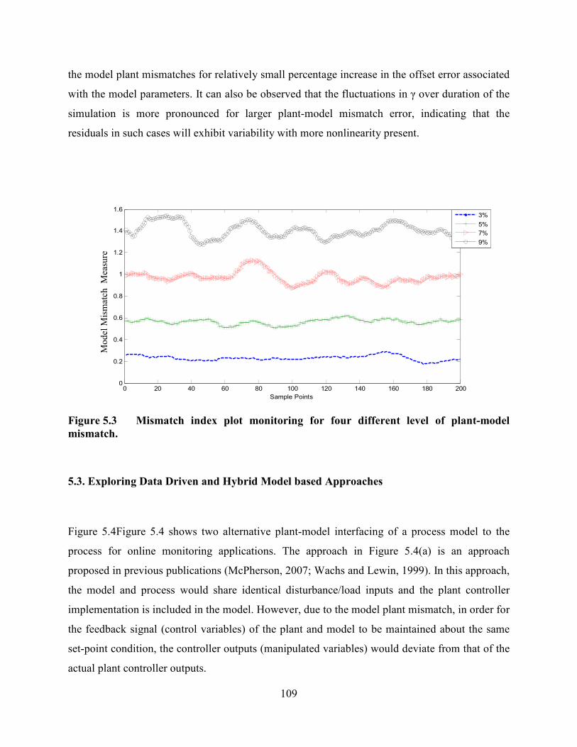
109

the model plant mismatches for relatively small percentage increase in the offset error associated

with the model parameters. It can also be observed that the fluctuations in γ over duration of the

simulation is more pronounced for larger plant-model mismatch error, indicating that the

residuals in such cases will exhibit variability with more nonlinearity present.

Figure 5.3 Mismatch index plot monitoring for four different level of plant-model

mismatch.

5.3. Exploring Data Driven and Hybrid Model based Approaches

Figure 5.4Figure 5.4 shows two alternative plant-model interfacing of a process model to the

process for online monitoring applications. The approach in Figure 5.4(a) is an approach

proposed in previous publications (McPherson, 2007; Wachs and Lewin, 1999). In this approach,

the model and process would share identical disturbance/load inputs and the plant controller

implementation is included in the model. However, due to the model plant mismatch, in order for

the feedback signal (control variables) of the plant and model to be maintained about the same

set-point condition, the controller outputs (manipulated variables) would deviate from that of the

actual plant controller outputs.

0 20 40 60 80 100 120 140 160 180 2000

0.2

0.4

0.6

0.8

1

1.2

1.4

1.6

Sample Points

Model Mis-math Measure

3%

5%

7%

9%

Mo

del

Mis

mat

ch

Mea

sure

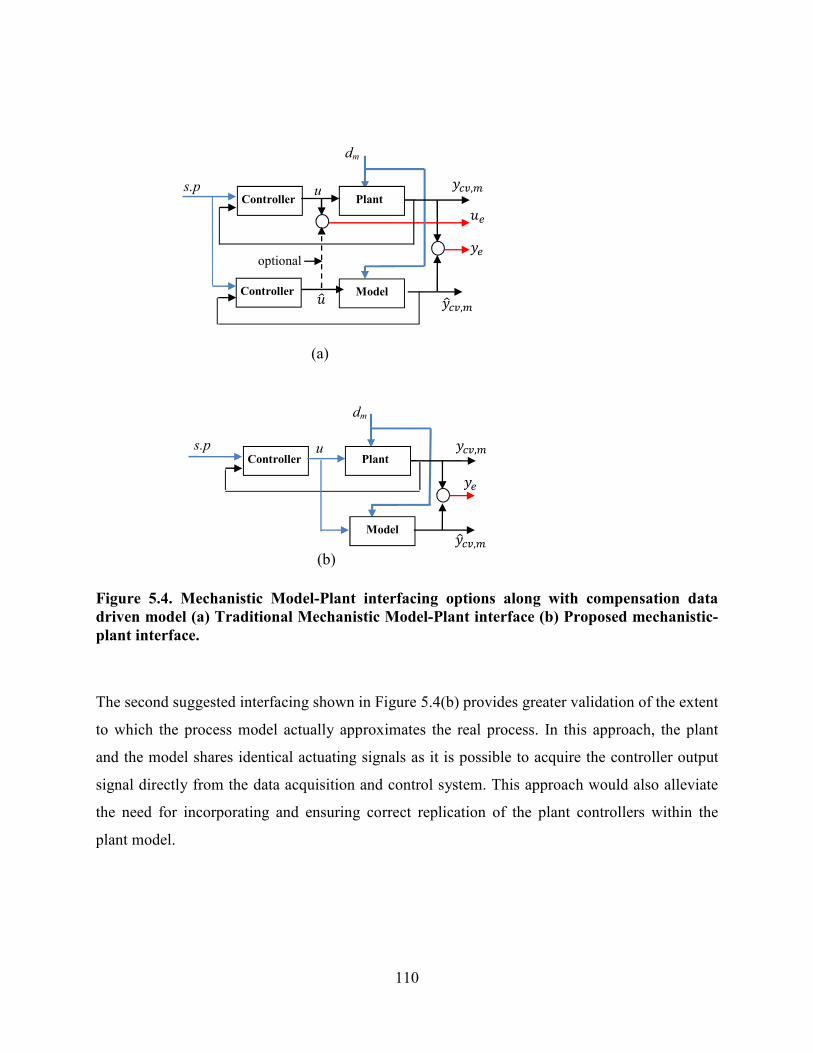
110

(a)

Figure 5.4. Mechanistic Model-Plant interfacing options along with compensation data

driven model (a) Traditional Mechanistic Model-Plant interface (b) Proposed mechanistic-

plant interface.

The second suggested interfacing shown in Figure 5.4(b) provides greater validation of the extent

to which the process model actually approximates the real process. In this approach, the plant

and the model shares identical actuating signals as it is possible to acquire the controller output

signal directly from the data acquisition and control system. This approach would also alleviate

the need for incorporating and ensuring correct replication of the plant controllers within the

plant model.

Controller

Controller Model

Plant

Controller

Model

Plant

optional

s.p u

dm

dm

u s.p

(b)

%ÃP>,@

%ÃP>,@

%P>,@

%P>,@

%7

Û7

%7

ÛÃ

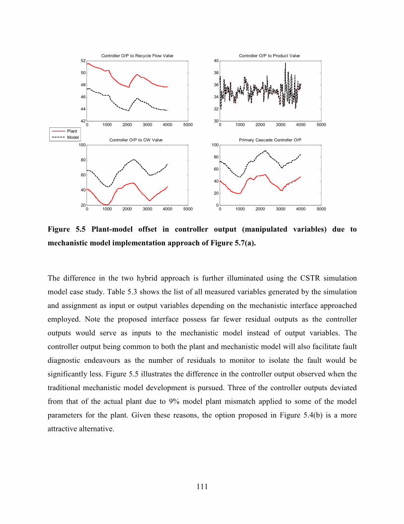
111

Figure 5.5 Plant-model offset in controller output (manipulated variables) due to

mechanistic model implementation approach of Figure 5.7(a).

The difference in the two hybrid approach is further illuminated using the CSTR simulation

model case study. Table 5.3 shows the list of all measured variables generated by the simulation

and assignment as input or output variables depending on the mechanistic interface approached

employed. Note the proposed interface possess far fewer residual outputs as the controller

outputs would serve as inputs to the mechanistic model instead of output variables. The

controller output being common to both the plant and mechanistic model will also facilitate fault

diagnostic endeavours as the number of residuals to monitor to isolate the fault would be

significantly less. Figure 5.5 illustrates the difference in the controller output observed when the

traditional mechanistic model development is pursued. Three of the controller outputs deviated

from that of the actual plant due to 9% model plant mismatch applied to some of the model

parameters for the plant. Given these reasons, the option proposed in Figure 5.4(b) is a more

attractive alternative.

0 1000 2000 3000 4000 500042

44

46

48

50

52Controller O/P to Recycle Flow Valve

0 1000 2000 3000 4000 500030

32

34

36

38

40Controller O/P to Product Valve

0 1000 2000 3000 4000 500020

40

60

80

100Controller O/P to CW Valve

0 1000 2000 3000 4000 50000

20

40

60

80

100Primary Cascade Controller O/P

Plant

Model

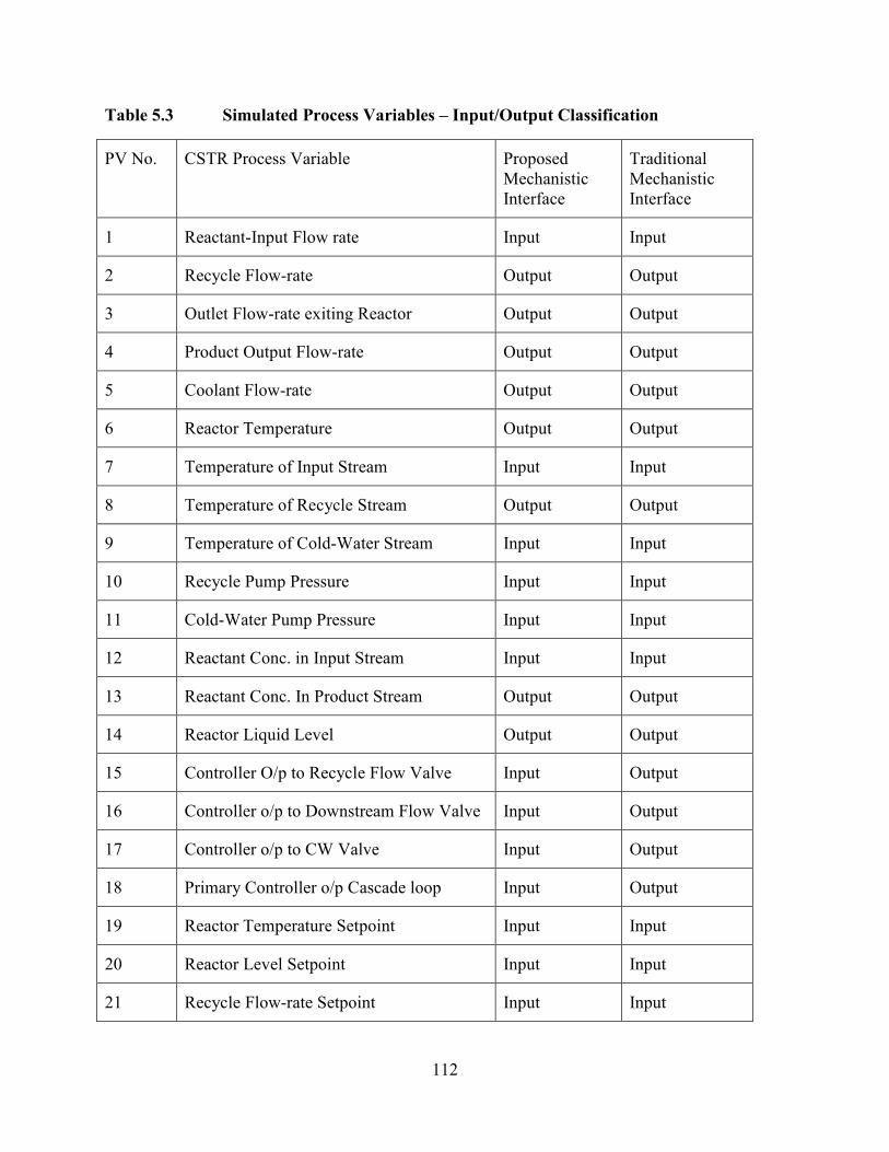
112

Table 5.3 Simulated Process Variables – Input/Output Classification

PV No. CSTR Process Variable Proposed

Mechanistic

Interface

Traditional

Mechanistic

Interface

1 Reactant-Input Flow rate Input Input

2 Recycle Flow-rate Output Output

3 Outlet Flow-rate exiting Reactor Output Output

4 Product Output Flow-rate Output Output

5 Coolant Flow-rate Output Output

6 Reactor Temperature Output Output

7 Temperature of Input Stream Input Input

8 Temperature of Recycle Stream Output Output

9 Temperature of Cold-Water Stream Input Input

10 Recycle Pump Pressure Input Input

11 Cold-Water Pump Pressure Input Input

12 Reactant Conc. in Input Stream Input Input

13 Reactant Conc. In Product Stream Output Output

14 Reactor Liquid Level Output Output

15 Controller O/p to Recycle Flow Valve Input Output

16 Controller o/p to Downstream Flow Valve Input Output

17 Controller o/p to CW Valve Input Output

18 Primary Controller o/p Cascade loop Input Output

19 Reactor Temperature Setpoint Input Input

20 Reactor Level Setpoint Input Input

21 Recycle Flow-rate Setpoint Input Input

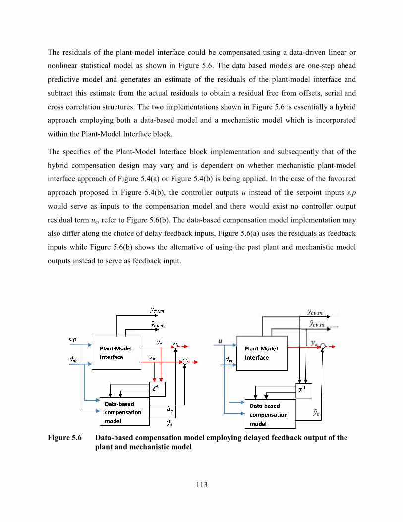
113

The residuals of the plant-model interface could be compensated using a data-driven linear or

nonlinear statistical model as shown in Figure 5.6. The data based models are one-step ahead

predictive model and generates an estimate of the residuals of the plant-model interface and

subtract this estimate from the actual residuals to obtain a residual free from offsets, serial and

cross correlation structures. The two implementations shown in Figure 5.6 is essentially a hybrid

approach employing both a data-based model and a mechanistic model which is incorporated

within the Plant-Model Interface block.

The specifics of the Plant-Model Interface block implementation and subsequently that of the

hybrid compensation design may vary and is dependent on whether mechanistic plant-model

interface approach of Figure 5.4(a) or Figure 5.4(b) is being applied. In the case of the favoured

approach proposed in Figure 5.4(b), the controller outputs u instead of the setpoint inputs s.p

would serve as inputs to the compensation model and there would exist no controller output

residual term ue, refer to Figure 5.6(b). The data-based compensation model implementation may

also differ along the choice of delay feedback inputs, Figure 5.6(a) uses the residuals as feedback

inputs while Figure 5.6(b) shows the alternative of using the past plant and mechanistic model

outputs instead to serve as feedback input.

(a) (b)

Figure 5.6 Data-based compensation model employing delayed feedback output of the

plant and mechanistic model

%ÃP>,@

%Ã7

%P>,@

114

All approaches described would ultimately derive a dynamic data-based model capable of

capturing what remaining structure is still retained in the residuals of the plant-mechanistic

model interface. For a dynamic system the current values of the variables are also dependent

upon the past values. Thus, the model would be required not only to capture the linear

relationship between X(t) but also X(t-1), X(t – 2), and so forth. PLS can be extended to dynamic

systems by carrying out a matrix expansion of the original data matrix with time-shifted

duplicate vectors. By appropriate selection of the number of lags l to be included X(t – l), both

the static and dynamic relationship between the variables can be captured.

Xd = [X(t-1) X(t-2) ……X(k-l)]

(5.10)

For the application reported in this paper, the X matrix composed of both input/disturbance

measurements and past time-delayed output variables(control, manipulated, and monitored

measurements). Implementation of a one-step ahead predictive model also meant that the

response vector or matrix Y would comprise of the set of output variables at the current time

instance:

Y = [Ym(t),Ycv(t),Ucv(t)]

(5.11)

where Ycv(t) is the set of contol variables and Ucv(t) is the set of manipulated input variables and

Ym(t) is the set of monitored output variables not belonging to the two previously stated groups.

The non-linear QPLS model employed the same set of data for its input (X) and outputs (Y)

matrix. In the case of the QPLS, several methods of parameterization of the quadratic inner

relation were explored based upon the original work of Wold et al.(1989) and three variants of

that approach investigated by Baffi et al.(1999b). All QPLS updating alternatives are linked by

the Newton-Raphson linearization of the quadratic inner relation and for this specific case study

there was no distinctive performance difference between the alternatives and so ultimately the

original algorithm by Wolds et al. (1989) was used. For both the linear and nonlinear QPLS

model the number of latent vectors employed by the model was automatically selected based

upon cross-validation and convergence specification tolerance.

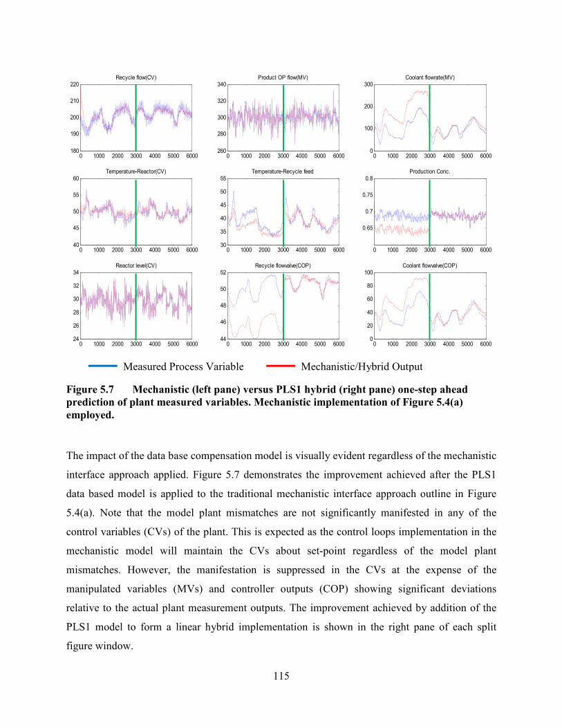
115

Figure 5.7 Mechanistic (left pane) versus PLS1 hybrid (right pane) one-step ahead

prediction of plant measured variables. Mechanistic implementation of Figure 5.4(a)

employed.

The impact of the data base compensation model is visually evident regardless of the mechanistic

interface approach applied. Figure 5.7 demonstrates the improvement achieved after the PLS1

data based model is applied to the traditional mechanistic interface approach outline in Figure

5.4(a). Note that the model plant mismatches are not significantly manifested in any of the

control variables (CVs) of the plant. This is expected as the control loops implementation in the

mechanistic model will maintain the CVs about set-point regardless of the model plant

mismatches. However, the manifestation is suppressed in the CVs at the expense of the

manipulated variables (MVs) and controller outputs (COP) showing significant deviations

relative to the actual plant measurement outputs. The improvement achieved by addition of the

PLS1 model to form a linear hybrid implementation is shown in the right pane of each split

figure window.

0 1000 2000 3000 4000 5000 6000180

190

200

210

220Recycle flow(CV)

0 1000 2000 3000 4000 5000 6000260

280

300

320

340Product OP flow(MV)

0 1000 2000 3000 4000 5000 60000

100

200

300Coolant flowrate(MV)

0 1000 2000 3000 4000 5000 600040

45

50

55

60Temperature-Reactor(CV)

0 1000 2000 3000 4000 5000 600030

35

40

45

50

55Temperature-Recycle feed

0 1000 2000 3000 4000 5000 6000

0.65

0.7

0.75

0.8Production Conc.

0 1000 2000 3000 4000 5000 600024

26

28

30

32

34Reactor level(CV)

0 1000 2000 3000 4000 5000 600044

46

48

50

52Recycle flowvalve(COP)

0 1000 2000 3000 4000 5000 60000

20

40

60

80

100Coolant flowvalve(COP)

Measured Process Variable Mechanistic/Hybrid Output

116

Even better results were obtained using the proposed mechanistic model interface strategy,

Figure 5.8 shows the before and after impact of incorporating the PLS1 model as a data-based

compensation model to implement an hybrid model, refer to Figure 5.6(b). In this approach the

plant-model mismatch is not masked by the control loop since its driven by the same control

output signals as the plant, hence there exist a more measurable difference between the plant and

model control variables (CVs). However, the compensation data base model is more effective

with this mechanistic interface approach because it is able to exploit the information content in

the controller output signal to provide better correction, estimation (one-step ahead predictive

tracking) of the other plant variables.

Figure 5.8 Mechanistic (left pane) vs PLS1 hybrid (right pane) prediction of plant

measured variables. Mechanistic implementation of Figure 5.4(b) employed.

Table 5.4 compares the mean square error of the measured residuals of the compensated (hybrid)

and uncompensated mechanistic model for both the traditional and proposed implementation.

From the analysis thus far it is clear that the mechanistic online monitoring interface approach

0 1000 2000 3000 4000 5000 6000180

190

200

210

220

230

240Recycle flow(CV)

0 1000 2000 3000 4000 5000 6000260

280

300

320

340Product OP flow(MV)

0 1000 2000 3000 4000 5000 60000

50

100

150

200

250Coolant flowrate(MV)

0 1000 2000 3000 4000 5000 600040

45

50

55

60Temperature-Reactor(CV)

0 1000 2000 3000 4000 5000 600030

35

40

45

50

55Temperature-Recycle feed

0 1000 2000 3000 4000 5000 60000.62

0.64

0.66

0.68

0.7

0.72

0.74Production Conc.

Measured Process Variable Mechanistic/Hybrid Output

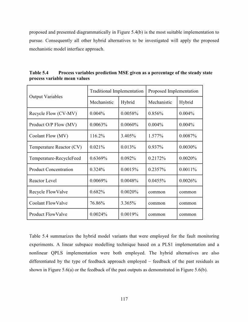
117

proposed and presented diagrammatically in Figure 5.4(b) is the most suitable implementation to

pursue. Consequently all other hybrid alternatives to be investigated will apply the proposed

mechanistic model interface approach.

Table 5.4 Process variables prediction MSE given as a percentage of the steady state

process variable mean values

Output Variables

Traditional Implementation Proposed Implementation

Mechanistic Hybrid Mechanistic Hybrid

Recycle Flow (CV-MV) 0.004% 0.0058% 0.856% 0.004%

Product O/P Flow (MV) 0.0063% 0.0060% 0.004% 0.004%

Coolant Flow (MV) 116.2% 3.405% 1.577% 0.0087%

Temperature Reactor (CV) 0.021% 0.013% 0.937% 0.0030%

Temperature-RecycleFeed 0.6369% 0.092% 0.2172% 0.0020%

Product Concentration 0.324% 0.0015% 0.2357% 0.0011%

Reactor Level 0.0069% 0.0048% 0.0455% 0.0026%

Recycle FlowValve 0.682% 0.0020% common common

Coolant FlowValve 76.86% 3.365% common common

Product FlowValve 0.0024% 0.0019% common common

Table 5.4 summarizes the hybrid model variants that were employed for the fault monitoring

experiments. A linear subspace modelling technique based on a PLS1 implementation and a

nonlinear QPLS implementation were both employed. The hybrid alternatives are also

differentiated by the type of feedback approach employed – feedback of the past residuals as

shown in Figure 5.6(a) or the feedback of the past outputs as demonstrated in Figure 5.6(b).

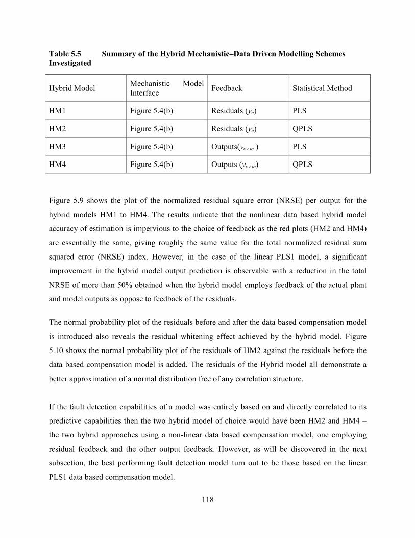
118

Table 5.5 Summary of the Hybrid Mechanistic–Data Driven Modelling Schemes

Investigated

Hybrid Model Mechanistic Model

Interface Feedback Statistical Method

HM1 Figure 5.4(b) Residuals (ye) PLS

HM2 Figure 5.4(b) Residuals (ye) QPLS

HM3 Figure 5.4(b) Outputs(ycv,m ) PLS

HM4 Figure 5.4(b) Outputs (ycv,m) QPLS

Figure 5.9 shows the plot of the normalized residual square error (NRSE) per output for the

hybrid models HM1 to HM4. The results indicate that the nonlinear data based hybrid model

accuracy of estimation is impervious to the choice of feedback as the red plots (HM2 and HM4)

are essentially the same, giving roughly the same value for the total normalized residual sum

squared error (NRSE) index. However, in the case of the linear PLS1 model, a significant

improvement in the hybrid model output prediction is observable with a reduction in the total

NRSE of more than 50% obtained when the hybrid model employs feedback of the actual plant

and model outputs as oppose to feedback of the residuals.

The normal probability plot of the residuals before and after the data based compensation model

is introduced also reveals the residual whitening effect achieved by the hybrid model. Figure

5.10 shows the normal probability plot of the residuals of HM2 against the residuals before the

data based compensation model is added. The residuals of the Hybrid model all demonstrate a

better approximation of a normal distribution free of any correlation structure.

If the fault detection capabilities of a model was entirely based on and directly correlated to its

predictive capabilities then the two hybrid model of choice would have been HM2 and HM4 –

the two hybrid approaches using a non-linear data based compensation model, one employing

residual feedback and the other output feedback. However, as will be discovered in the next

subsection, the best performing fault detection model turn out to be those based on the linear

PLS1 data based compensation model.

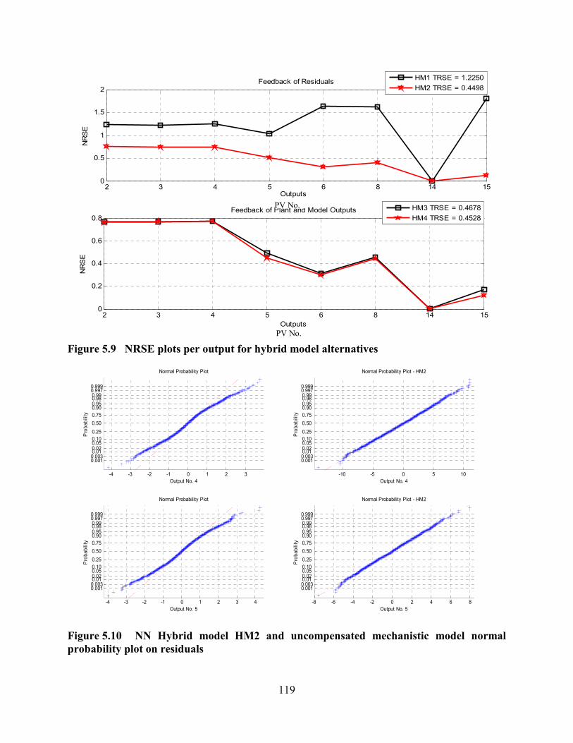
119

Figure 5.9 NRSE plots per output for hybrid model alternatives

Figure 5.10 NN Hybrid model HM2 and uncompensated mechanistic model normal

probability plot on residuals

2 3 4 5 6 8 14 150

0.5

1

1.5

2

Outputs

NRSE

Feedback of Residuals

2 3 4 5 6 8 14 150

0.2

0.4

0.6

0.8

Outputs

NRSE

Feedback of Plant and Model Outputs

HM1 TRSE = 1.2250

HM2 TRSE = 0.4498

HM3 TRSE = 0.4678

HM4 TRSE = 0.4528

-4 -3 -2 -1 0 1 2 3

0.0010.0030.01 0.02 0.05 0.10

0.25

0.50

0.75

0.90 0.95 0.98 0.99 0.9970.999

Output No. 4

Probability

Normal Probability Plot

-10 -5 0 5 10

0.0010.0030.01 0.02 0.05 0.10

0.25

0.50

0.75

0.90 0.95 0.98 0.99 0.9970.999

Output No. 4

Probability

Normal Probability Plot - HM2

-4 -3 -2 -1 0 1 2 3 4

0.0010.0030.01 0.02 0.05 0.10

0.25

0.50

0.75

0.90 0.95 0.98 0.99 0.9970.999

Output No. 5

Probability

Normal Probability Plot

-8 -6 -4 -2 0 2 4 6 8

0.0010.0030.01 0.02 0.05 0.10

0.25

0.50

0.75

0.90 0.95 0.98 0.99 0.9970.999

Output No. 5

Probability

Normal Probability Plot - HM2

PV No.

PV No.

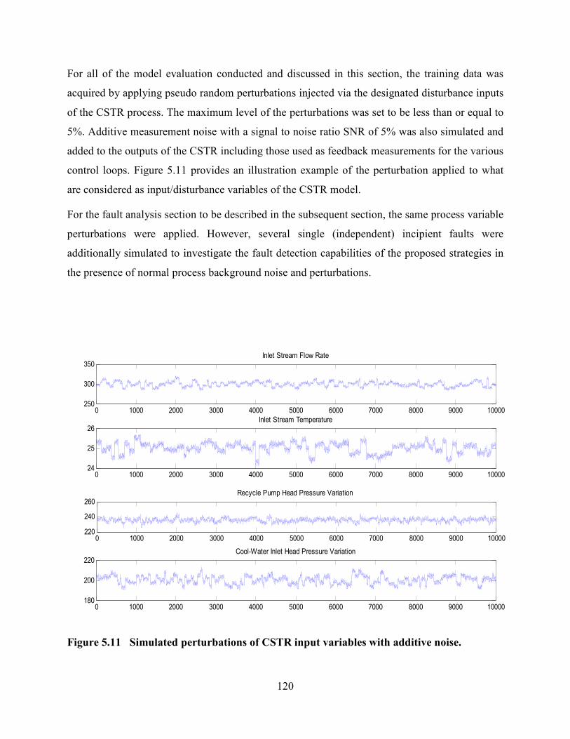
120

For all of the model evaluation conducted and discussed in this section, the training data was

acquired by applying pseudo random perturbations injected via the designated disturbance inputs

of the CSTR process. The maximum level of the perturbations was set to be less than or equal to

5%. Additive measurement noise with a signal to noise ratio SNR of 5% was also simulated and

added to the outputs of the CSTR including those used as feedback measurements for the various

control loops. Figure 5.11 provides an illustration example of the perturbation applied to what

are considered as input/disturbance variables of the CSTR model.

For the fault analysis section to be described in the subsequent section, the same process variable

perturbations were applied. However, several single (independent) incipient faults were

additionally simulated to investigate the fault detection capabilities of the proposed strategies in

the presence of normal process background noise and perturbations.

Figure 5.11 Simulated perturbations of CSTR input variables with additive noise.

0 1000 2000 3000 4000 5000 6000 7000 8000 9000 10000250

300

350Inlet Stream Flow Rate

0 1000 2000 3000 4000 5000 6000 7000 8000 9000 1000024

25

26Inlet Stream Temperature

Cool-Water Temperature

0 1000 2000 3000 4000 5000 6000 7000 8000 9000 10000220

240

260Recycle Pump Head Pressure Variation

0 1000 2000 3000 4000 5000 6000 7000 8000 9000 10000180

200

220Cool-Water Inlet Head Pressure Variation

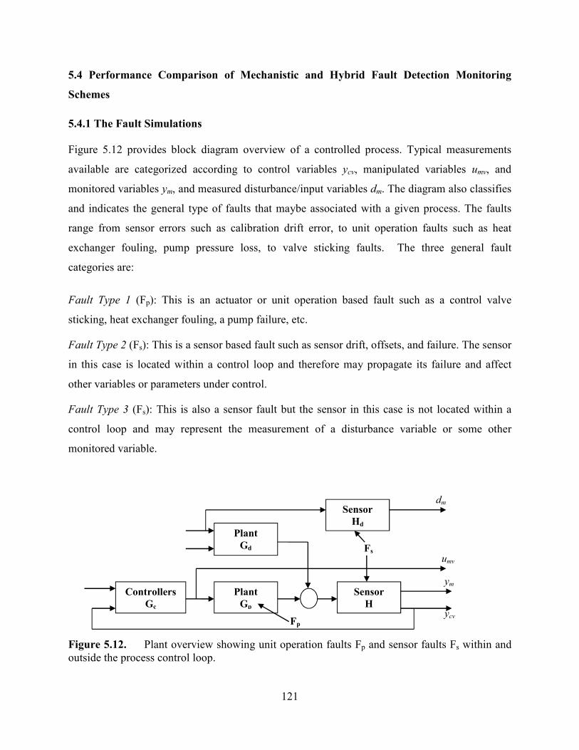
121

5.4 Performance Comparison of Mechanistic and Hybrid Fault Detection Monitoring

Schemes

5.4.1 The Fault Simulations

Figure 5.12 provides block diagram overview of a controlled process. Typical measurements

available are categorized according to control variables ycv, manipulated variables umv, and

monitored variables ym, and measured disturbance/input variables dm. The diagram also classifies

and indicates the general type of faults that maybe associated with a given process. The faults

range from sensor errors such as calibration drift error, to unit operation faults such as heat

exchanger fouling, pump pressure loss, to valve sticking faults. The three general fault

categories are:

Fault Type 1 (Fp): This is an actuator or unit operation based fault such as a control valve

sticking, heat exchanger fouling, a pump failure, etc.

Fault Type 2 (Fs): This is a sensor based fault such as sensor drift, offsets, and failure. The sensor

in this case is located within a control loop and therefore may propagate its failure and affect

other variables or parameters under control.

Fault Type 3 (Fs): This is also a sensor fault but the sensor in this case is not located within a

control loop and may represent the measurement of a disturbance variable or some other

monitored variable.

Figure 5.12. Plant overview showing unit operation faults Fp and sensor faults Fs within and

outside the process control loop.

Controllers

Gc

Plant

Gp

Sensor

H

Plant

Gd

Sensor

Hd

Fs

Fp

dm

umv

ym

ycv

122

The manifestation of the faults in terms of process variables affected was dependent upon the

type of fault and its location. Faults generated within control loops, be it of the sensor or unit

operation type, tend to be more readily detected because of the propagating effect of the control

loop. Other faults resulted in more subtle shift in the mean level of the auto-scaled process

variables which would not be easily detected by an operator, relying on visual observation of

trend charts, until perhaps the fault magnitude was much more severe. An example of such a

fault scenario is shown in Figure 5.13(a), this is a developing pipe blockage fault and can only be

observed to impact the mean deviation on the downstream flow controller output signal to the

valve.

The valve sticking faults are of a dynamic nature and were only detectable under significant

valve stem movement. The example provided in

Figure 5.13Figure 5.13(b) is shown to generate unstable oscillatory effects, impacting the

frequency content and standard deviation spread of the process variables affected.

The effect of a given fault on the process variable deviation, as shown in the two examples

provided, can be very subtle and difficult to detect by mere visual monitoring of one or more of

the process variables. An effective model-based fault monitoring system should, however, be

able to detect such faults and do so within an acceptable time window relative to the onset of the

fault. Subsequently, the time delay to the detection of a fault will be one of the key metrics used

to evaluate the performance of the proposed hybrid schemes that will follow in the proceeding

sections. It can also be observed that the impact of the fault on the monitored process variables is

dependent on the specific fault in terms of its location and type. Case in point, the cool-water

valve sticking fault impact is most visible via the onset of oscillation in the cool-water flow-rate

measurements whereas the pipe blocking fault effect is more subtle and does not result in the

onset of any oscillation.

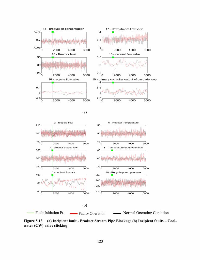
123

(a)

(b)

Figure 5.13 (a) Incipient fault - Product Stream Pipe Blockage (b) Incipient faults – Cool-

water (CW) valve sticking

0 2000 4000 60000.65

0.7

0.7514 - production concentration

0 2000 4000 600025

30

3515 - Reactor level

0 2000 4000 60004.9

5

5.1

16 - recycle flow valve

0 2000 4000 60003

3.5

417 - downstream flow valve

0 2000 4000 60002.5

3

3.518 - coolant flow valve

0 2000 4000 60002.5

3

3.5

419 - primary controller output of cascade loop

0 2000 4000 6000190

200

2102 - recycle flow

0 2000 4000 6000250

300

3504 - product output flow

0 2000 4000 600060

80

1005 - coolant flowrate

0 2000 4000 600045

50

556 - Reactor Temperature

0 2000 4000 600035

40

458 - Temperature of recycle feed

0 2000 4000 6000220

230

240

25010 - Recycle pump pressure

Faulty Operation Normal Operating Condition Fault Initiation Pt.

124

All faults were initiated at sample instance 1500. The incipient type faults were implemented

using a constant drift percentage to produce a linear deviation from the true nominal reading over

time. The incipient grow rate of the simulated faults differed, however, all sensor faults were

implemented such that the maximum deviation at the end of each simulation run (5500 samples)

was set to 10% of the measured process variable nominal value. Table 5.16 gives a list of the

faults simulated and the fault type category classification of each.

Table 5.6 Simulated Fault Summary

Fault No. Fault Description Fault Type

1 Reactor temp. sensor drift 2

2 Reactant input stream temp. sensor drift 3

3 Recycle temp. sensor drift 3

4 CW feed temperature sensor drift 3

5 Recycle pump pressure sensor drift 3

6 CW feed pump pressure sensor drift 3

7 Reactor level sensor 2

8 Input stream - flow sensor drift 3

9 Recycle loop - flow sensor drift 2

10 Product-output flow sensor drift 3

11 Cool-water flow sensor drift 2

12 Heat exchanger fowling 1

13 Pipe Blockage-Recycle loop 1

14 Pipe Blockage-Product Stream 1

15 Pipe Blockage-CoolingWater Feed 1

16 Recycle Pump Failure 1

17 Valve Sticking – CoolWater Valve 1

18 Valve Sticking – Product Valve 1

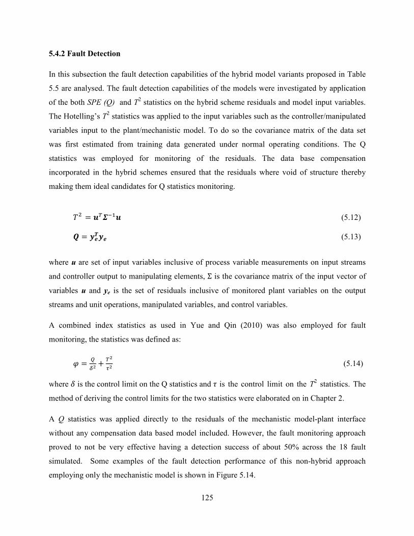
125

5.4.2 Fault Detection

In this subsection the fault detection capabilities of the hybrid model variants proposed in Table

5.5 are analysed. The fault detection capabilities of the models were investigated by application

of the both SPE (Q) and T2 statistics on the hybrid scheme residuals and model input variables.

The Hotelling’s T2 statistics was applied to the input variables such as the controller/manipulated

variables input to the plant/mechanistic model. To do so the covariance matrix of the data set

was first estimated from training data generated under normal operating conditions. The Q

statistics was employed for monitoring of the residuals. The data base compensation

incorporated in the hybrid schemes ensured that the residuals where void of structure thereby

making them ideal candidates for Q statistics monitoring.

r? = _�]�1_ (5.12)

x = ¢qo¢q (5.13)

where u are set of input variables inclusive of process variable measurements on input streams

and controller output to manipulating elements, Σ is the covariance matrix of the input vector of

variables u and ye is the set of residuals inclusive of monitored plant variables on the output

streams and unit operations, manipulated variables, and control variables.

A combined index statistics as used in Yue and Qin (2010) was also employed for fault

monitoring, the statistics was defined as:

^ = _`J + �J

J )))))))))))))))))))))))))))))))))))))))))))))))))))))))))))))))))))))))))))))))))))))))))))))))))))))))))))))))))))))))))))))))))(5.14)

where a is the control limit on the Q statistics and , is the control limit on the T2 statistics. The

method of deriving the control limits for the two statistics were elaborated on in Chapter 2.

A Q statistics was applied directly to the residuals of the mechanistic model-plant interface

without any compensation data based model included. However, the fault monitoring approach

proved to not be very effective having a detection success of about 50% across the 18 fault

simulated. Some examples of the fault detection performance of this non-hybrid approach

employing only the mechanistic model is shown in Figure 5.14.

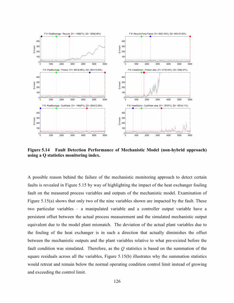
126

Figure 5.14 Fault Detection Performance of Mechanistic Model (non-hybrid approach)

using a Q statistics monitoring index.

A possible reason behind the failure of the mechanistic monitoring approach to detect certain

faults is revealed in Figure 5.15 by way of highlighting the impact of the heat exchanger fouling

fault on the measured process variables and outputs of the mechanistic model. Examination of

Figure 5.15(a) shows that only two of the nine variables shown are impacted by the fault. These

two particular variables – a manipulated variable and a controller output variable have a

persistent offset between the actual process measurement and the simulated mechanistic output

equivalent due to the model plant mismatch. The deviation of the actual plant variables due to

the fouling of the heat exchanger is in such a direction that actually diminishes the offset

between the mechanistic outputs and the plant variables relative to what pre-existed before the

fault condition was simulated. Therefore, as the Q statistics is based on the summation of the

square residuals across all the variables, Figure 5.15(b) illustrates why the summation statistics

would retreat and remain below the normal operating condition control limit instead of growing

and exceeding the control limit.

0 1000 2000 3000 4000 5000 60000

100

200

300

400

Q-mean

F13 -PipeBlockage - Recycle, D1= -1368(F%), D2= 1200(2.66%)

0 1000 2000 3000 4000 5000 60000

100

200

300

400

Q-mean

F14 -PipeBlockage - Product, D1= 3091(6.86%), D2= 4501(10.00%)

0 1000 2000 3000 4000 5000 60000

100

200

300

400

Q-mean

F15 -PipeBlockage - CoolWater, D1= -1464(F%), D2= 2834(12.59%)

0 1000 2000 3000 4000 5000 60000

100

200

300

400

Q-mean

F16 -Recycle Pump Failure, D1= 825(1.83%), D2= 4501(10.00%)

0 1000 2000 3000 4000 5000 60000

100

200

300

400

Q-mean

F18 -ValveStickin - Product valve, D1= 217(0.43%), D2= 239(0.47%)

0 1000 2000 3000 4000 5000 60000

100

200

300

400

Q-mean

F19 -ValveStickin - CoolWater valve, D1= -787(F%), D2= 1851(4.11%)

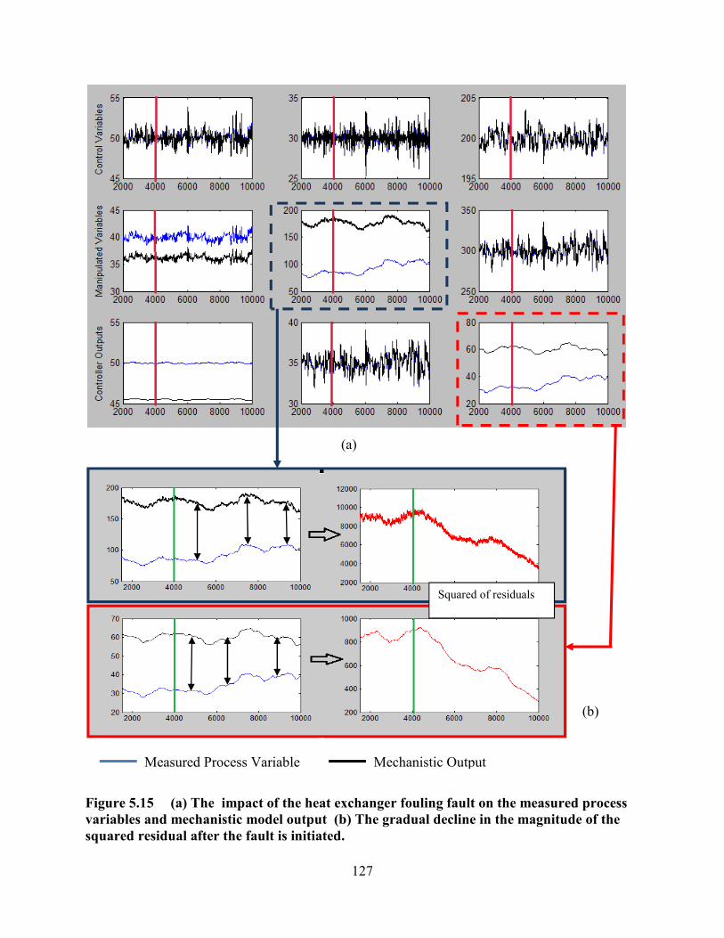
127

(a)

Figure 5.15 (a) The impact of the heat exchanger fouling fault on the measured process

variables and mechanistic model output (b) The gradual decline in the magnitude of the

squared residual after the fault is initiated.

(b)

Measured Process Variable Mechanistic Output

Squared of residuals

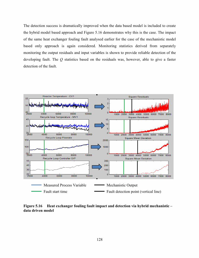
128

The detection success is dramatically improved when the data based model is included to create

the hybrid model based approach and Figure 5.16 demonstrates why this is the case. The impact

of the same heat exchanger fouling fault analysed earlier for the case of the mechanistic model

based only approach is again considered. Monitoring statistics derived from separately

monitoring the output residuals and input variables is shown to provide reliable detection of the

developing fault. The Q statistics based on the residuals was, however, able to give a faster

detection of the fault.

Figure 5.16 Heat exchanger fouling fault impact and detection via hybrid mechanistic –

data driven model

Measured Process Variable Mechanistic Output

Fault start time Fault detection point (vertical line)

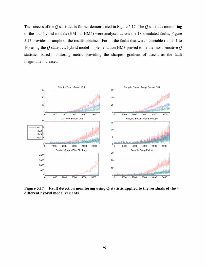
129

The success of the Q statistics is further demonstrated in Figure 5.17. The Q statistics monitoring

of the four hybrid models (HM1 to HM4) were analysed across the 18 simulated faults, Figure

5.17 provides a sample of the results obtained. For all the faults that were detectable (faults 1 to

16) using the Q statistics, hybrid model implementation HM3 proved to be the most sensitive Q

statistics based monitoring metric providing the sharpest gradient of ascent as the fault

magnitude increased.

Figure 5.17 Fault detection monitoring using Q statistic applied to the residuals of the 4

different hybrid model variants.

0 1000 2000 3000 4000 50000

20

40

60Reactor Temp. Sensor Drift

0 1000 2000 3000 4000 50000

20

40

60Recycle Stream Temp. Sensor Drift

0 1000 2000 3000 4000 50000

5

10

15

20CW Flow Sensor Drift

0 1000 2000 3000 4000 50000

5

10

15

Recycle Stream Pipe Blockage

0 1000 2000 3000 4000 50000

1000

2000

3000

4000

Product Stream Pipe Blockage

0 1000 2000 3000 4000 50000

10

20

30Recycle Pump Failure

HM1

HM2

HM3

HM4

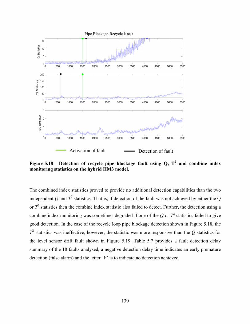
130

Figure 5.18 Detection of recycle pipe blockage fault using Q, T2 and combine index

monitoring statistics on the hybrid HM3 model.

The combined index statistics proved to provide no additional detection capabilities than the two

independent Q and T2 statistics. That is, if detection of the fault was not achieved by either the Q

or T2 statistics then the combine index statistic also failed to detect. Further, the detection using a

combine index monitoring was sometimes degraded if one of the Q or T2 statistics failed to give

good detection. In the case of the recycle loop pipe blockage detection shown in Figure 5.18, the

T2 statistics was ineffective, however, the statistic was more responsive than the Q statistics for

the level sensor drift fault shown in Figure 5.19. Table 5.7 provides a fault detection delay

summary of the 18 faults analysed, a negative detection delay time indicates an early premature

detection (false alarm) and the letter “F’ is to indicate no detection achieved.

0 500 1000 1500 2000 2500 3000 3500 4000 4500 5000 55000

5

10

15Q Statistics

Heat Exchanger Fowling Fault

0 500 1000 1500 2000 2500 3000 3500 4000 4500 5000 55000

50

100

150

200

T2 Statistics

0 500 1000 1500 2000 2500 3000 3500 4000 4500 5000 55000

1

2

3

T2Q Statistics

Pipe Blockage-Recycle loop

Activation of fault Detection of fault

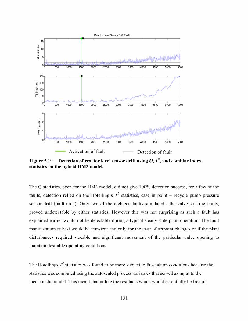
131

Figure 5.19 Detection of reactor level sensor drift using Q, T2, and combine index

statistics on the hybrid HM3 model.

The Q statistics, even for the HM3 model, did not give 100% detection success, for a few of the

faults, detection relied on the Hotelling’s T2 statistics, case in point – recycle pump pressure

sensor drift (fault no.5). Only two of the eighteen faults simulated - the valve sticking faults,

proved undetectable by either statistics. However this was not surprising as such a fault has

explained earlier would not be detectable during a typical steady state plant operation. The fault

manifestation at best would be transient and only for the case of setpoint changes or if the plant

disturbances required sizeable and significant movement of the particular valve opening to

maintain desirable operating conditions

The Hotellings T2 statistics was found to be more subject to false alarm conditions because the

statistics was computed using the autoscaled process variables that served as input to the

mechanistic model. This meant that unlike the residuals which would essentially be free of

0 500 1000 1500 2000 2500 3000 3500 4000 4500 5000 55000

5

10

15

Q Statistics

Reactor Level Sensor Drift Fault

0 500 1000 1500 2000 2500 3000 3500 4000 4500 5000 55000

50

100

150

200

T2 Statistics

0 500 1000 1500 2000 2500 3000 3500 4000 4500 5000 55000

1

2

3

T2Q Statistics

Activation of fault Detection of fault

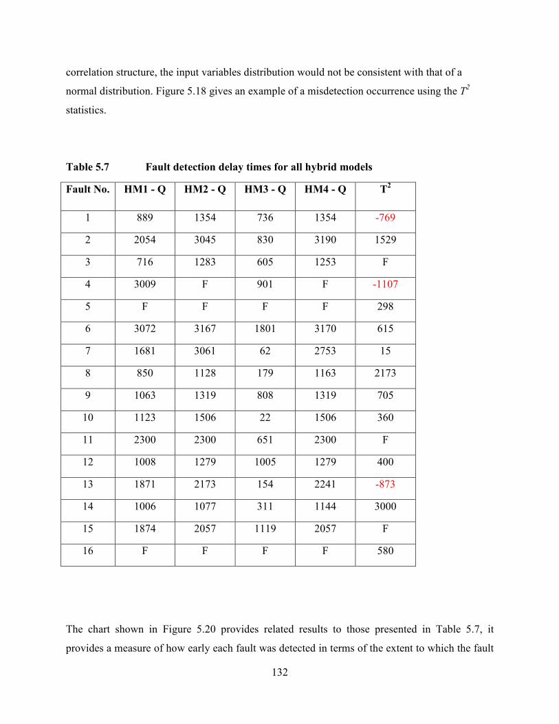
132

correlation structure, the input variables distribution would not be consistent with that of a

normal distribution. Figure 5.18 gives an example of a misdetection occurrence using the T2

statistics.

Table 5.7 Fault detection delay times for all hybrid models

Fault No. HM1 - Q HM2 - Q HM3 - Q HM4 - Q T2

1 889 1354 736 1354 -769

2 2054 3045 830 3190 1529

3 716 1283 605 1253 F

4 3009 F 901 F -1107

5 F F F F 298

6 3072 3167 1801 3170 615

7 1681 3061 62 2753 15

8 850 1128 179 1163 2173

9 1063 1319 808 1319 705

10 1123 1506 22 1506 360

11 2300 2300 651 2300 F

12 1008 1279 1005 1279 400

13 1871 2173 154 2241 -873

14 1006 1077 311 1144 3000

15 1874 2057 1119 2057 F

16 F F F F 580

The chart shown in Figure 5.20 provides related results to those presented in Table 5.7, it

provides a measure of how early each fault was detected in terms of the extent to which the fault

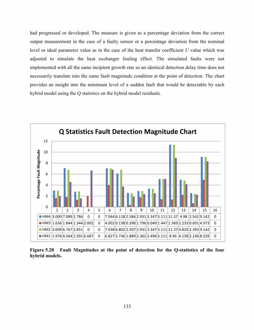
133

had progressed or developed. The measure is given as a percentage deviation from the correct

output measurement in the case of a faulty sensor or a percentage deviation from the nominal

level or ideal parameter value as in the case of the heat transfer coefficient U value which was

adjusted to simulate the heat exchanger fouling effect. The simulated faults were not

implemented with all the same incipient growth rate so an identical detection delay time does not

necessarily translate into the same fault magnitude condition at the point of detection. The chart

provides an insight into the minimum level of a sudden fault that would be detectable by each

hybrid model using the Q statistics on the hybrid model residuals.

Figure 5.20 Fault Magnitudes at the point of detection for the Q-statistics of the four

hybrid models.

1 2 3 4 5 6 7 8 9 10 11 12 13 14 15 16

HM4 3.009 7.089 2.784 0 0 7.044 6.118 2.584 2.931 3.347 5.111 11.37 4.98 2.542 9.142 0

HM3 1.636 1.844 1.344 2.002 0 4.002 0.138 0.398 1.796 0.049 1.447 1.369 2.233 0.691 4.973 0

HM2 3.009 6.767 2.851 0 0 7.038 6.802 2.507 2.931 3.347 5.111 11.37 4.829 2.393 9.142 0

HM1 1.976 4.564 1.591 6.687 0 6.827 3.736 1.889 2.362 2.496 5.111 8.96 4.158 2.236 8.329 0

0

2

4

6

8

10

12

Pe

rce

nta

ge

Fa

ult

Ma

gn

itu

de

Q Statistics Fault Detection Magnitude Chart

134

5.5 Distillation column, hybrid model, and disturbance overview

A simple dynamic distillation process model was developed using CHEMCAD to investigate the

fault/disturbance detection performance using a hybrid data driven model architecture and its

applicability to distillation column monitoring. Three independent feed condition changes were

simulated:

i) change in feed flow rate

ii) change in feed composition

iii) change in feed temperature

Sufficiently severe enough changes in any of the above three conditions can lead to column

flooding – vapour or liquid flooding condition. Also investigated was the effect of the combine

fault scenarios:

i) simultaneous change in feed flowrate and temperature

ii) simultaneous change in feed temperature and composition

The purpose of this particular case study was to investigate the applicability of hybrid

approaches which do not incorporate a mechanistic or first principle model of the plant. Quite

often developing a sufficiently accurate mechanistic model is not feasible for many real life

applications. This may be the case either because of insufficient information about the plant

dynamics or due to the sheer complexity of the plant, such undertaking might be too costly and

time consuming. As such the hybrid model implementation employed for fault monitoring for

the case study employed the use of a NN model and multiple ordinary least squares (OLS)

regression models. The objective being to approximate a quasi time-variant model by developing

several localised OLS models optimized about different operating points for the plant. The

artificial neural network model was use to provide a mapping between the coefficients of the

OLS models for the various operating points of the plant. The NN model therefore essential

serves the function of switching in the appropriate OLS model based upon the observed short-

term mean value of select process variables used to identified the current operating point of the

plant. Further details and results into the implementation of the column and faults, hybrid model,

and fault detection performance will be provided in the subsequent subsections to follow.

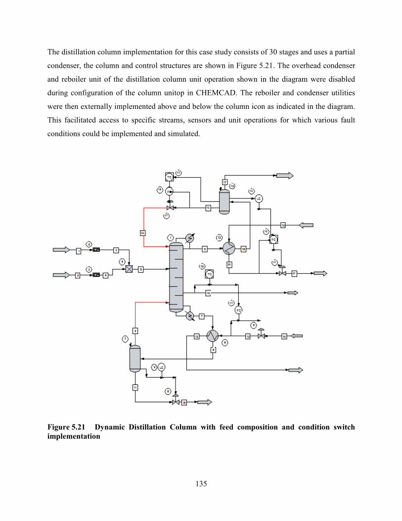
135

The distillation column implementation for this case study consists of 30 stages and uses a partial

condenser, the column and control structures are shown in Figure 5.21. The overhead condenser

and reboiler unit of the distillation column unit operation shown in the diagram were disabled

during configuration of the column unitop in CHEMCAD. The reboiler and condenser utilities

were then externally implemented above and below the column icon as indicated in the diagram.

This facilitated access to specific streams, sensors and unit operations for which various fault

conditions could be implemented and simulated.

Figure 5.21 Dynamic Distillation Column with feed composition and condition switch

implementation

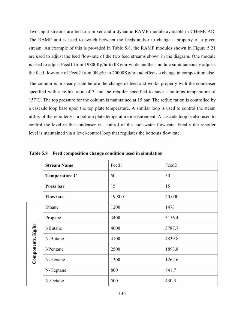
136

Two input streams are fed to a mixer and a dynamic RAMP module available in CHEMCAD.

The RAMP unit is used to switch between the feeds and/or to change a property of a given

stream. An example of this is provided in Table 5.8, the RAMP modules shown in Figure 5.21

are used to adjust the feed flow-rate of the two feed streams shown in the diagram. One module

is used to adjust Feed1 from 19800Kg/hr to 0Kg/hr while another module simultaneously adjusts

the feed flow-rate of Feed2 from 0Kg/hr to 20000Kg/hr and effects a change in composition also.

The column is in steady state before the change of feed and works properly with the condenser

specified with a reflux ratio of 3 and the reboiler specified to have a bottoms temperature of

157оC. The top pressure for the column is maintained at 15 bar. The reflux ration is controlled by

a cascade loop base upon the top plate temperature. A similar loop is used to control the steam

utility of the reboiler via a bottom plate temperature measurement. A cascade loop is also used to

control the level in the condenser via control of the cool-water flow-rate. Finally the reboiler

level is maintained via a level-control loop that regulates the bottoms flow rate.

Table 5.8 Feed composition change condition used in simulation

Stream Name Feed1 Feed2

Temperature C 50 50

Press bar 15 15

Flowrate 19,800 20,000

Co

mp

on

ents

, K

g/h

r

Ethane 1200 1473

Propane 3400 3156.4

I-Butane 4000 3787.7

N-Butane 4100 4839.8

I-Pentane 2500 1893.8

N-Hexane 1300 1262.6

N-Heptane 800 841.7

N-Octane 500 430.3

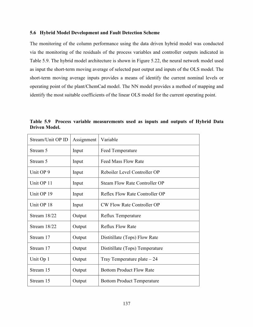
137

5.6 Hybrid Model Development and Fault Detection Scheme

The monitoring of the column performance using the data driven hybrid model was conducted

via the monitoring of the residuals of the process variables and controller outputs indicated in

Table 5.9. The hybrid model architecture is shown in Figure 5.22, the neural network model used

as input the short-term moving average of selected past output and inputs of the OLS model. The

short-term moving average inputs provides a means of identify the current nominal levels or

operating point of the plant/ChemCad model. The NN model provides a method of mapping and

identify the most suitable coefficients of the linear OLS model for the current operating point.

Table 5.9 Process variable measurements used as inputs and outputs of Hybrid Data

Driven Model.

Stream/Unit OP ID Assignment Variable

Stream 5 Input Feed Temperature

Stream 5 Input Feed Mass Flow Rate

Unit OP 9 Input Reboiler Level Controller OP

Unit OP 11 Input Steam Flow Rate Controller OP

Unit OP 19 Input Reflex Flow Rate Controller OP

Unit OP 18 Input CW Flow Rate Controller OP

Stream 18/22 Output Reflux Temperature

Stream 18/22 Output Reflux Flow Rate

Stream 17 Output Distitillate (Tops) Flow Rate

Stream 17 Output Distitillate (Tops) Temperature

Unit Op 1 Output Tray Temperature plate – 24

Stream 15 Output Bottom Product Flow Rate

Stream 15 Output Bottom Product Temperature

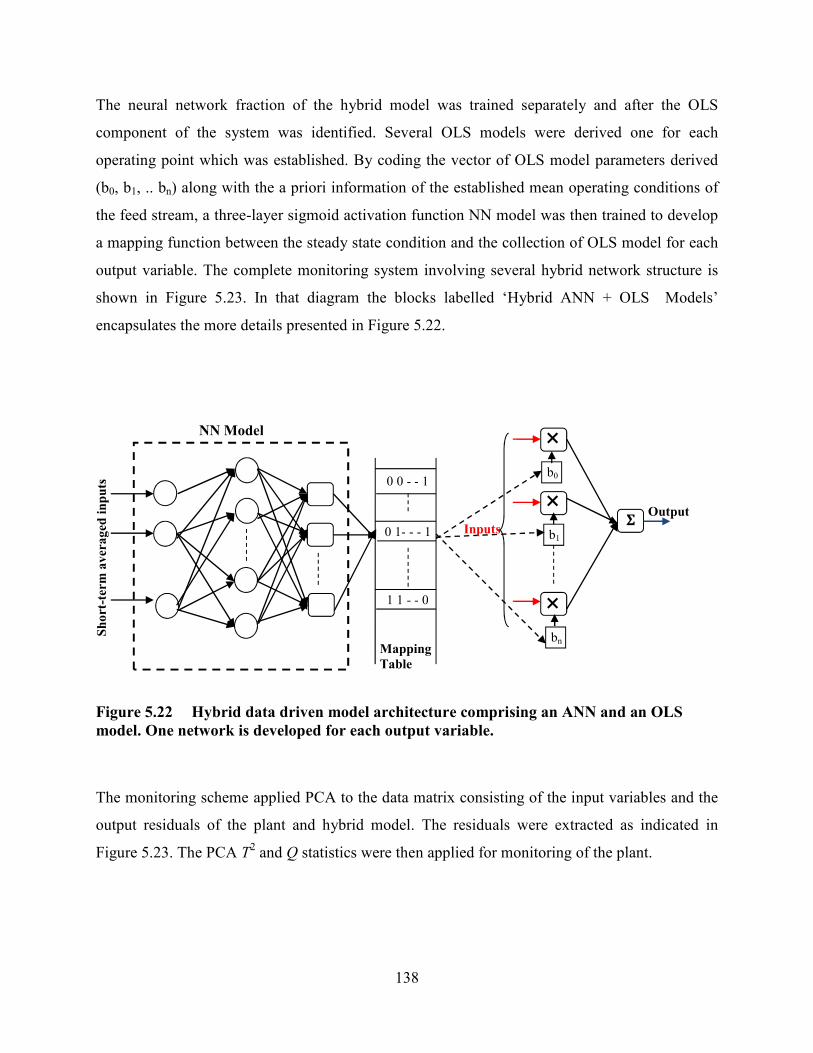
138

The neural network fraction of the hybrid model was trained separately and after the OLS

component of the system was identified. Several OLS models were derived one for each

operating point which was established. By coding the vector of OLS model parameters derived

(b0, b1, .. bn) along with the a priori information of the established mean operating conditions of

the feed stream, a three-layer sigmoid activation function NN model was then trained to develop

a mapping function between the steady state condition and the collection of OLS model for each

output variable. The complete monitoring system involving several hybrid network structure is

shown in Figure 5.23. In that diagram the blocks labelled ‘Hybrid ANN + OLS Models’

encapsulates the more details presented in Figure 5.22.

Figure 5.22 Hybrid data driven model architecture comprising an ANN and an OLS

model. One network is developed for each output variable.

The monitoring scheme applied PCA to the data matrix consisting of the input variables and the

output residuals of the plant and hybrid model. The residuals were extracted as indicated in

Figure 5.23. The PCA T2 and Q statistics were then applied for monitoring of the plant.

0 1- - - 1

0 0 - - 1

1 1 - - 0

b0

b1

bn

�

Mapping

Table

Inputs

NN Model

Output

Sh

ort

-ter

m a

ver

ag

ed i

np

uts

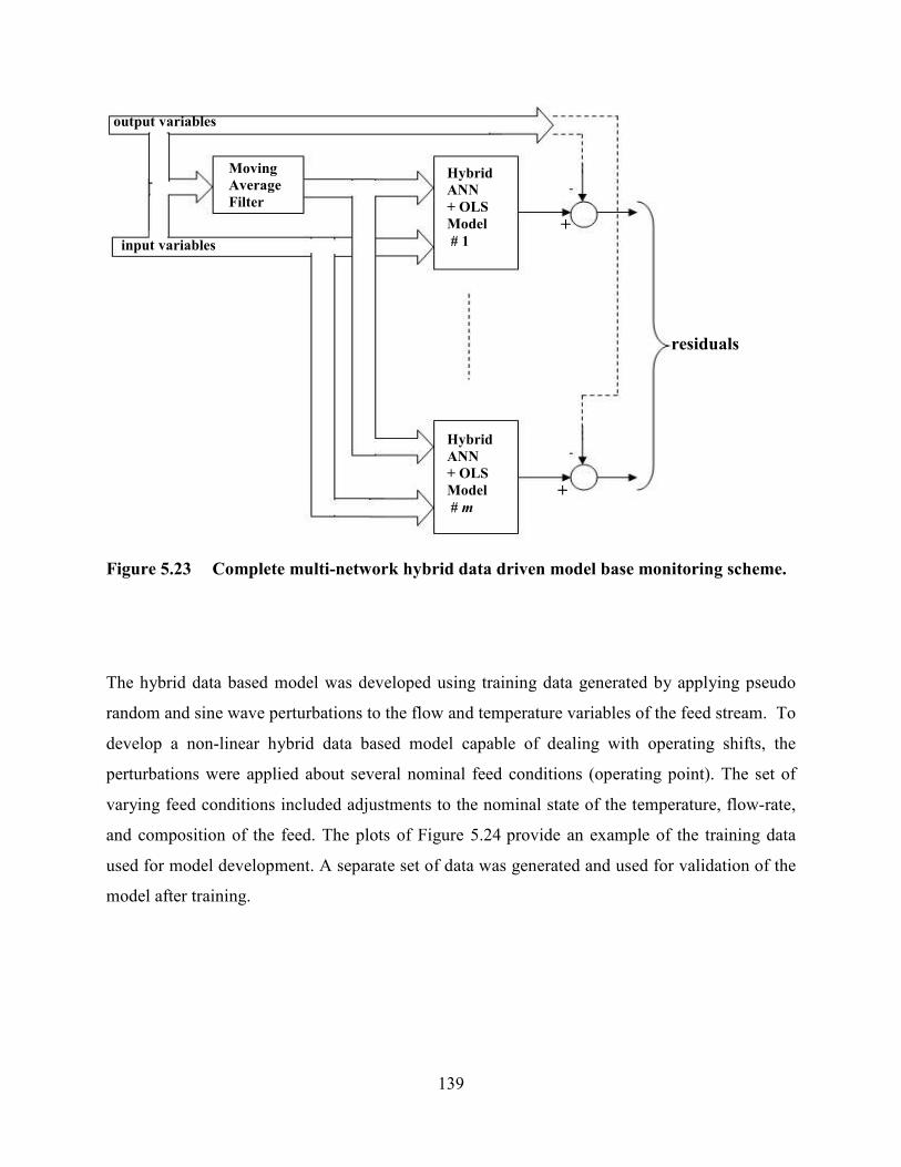
139

Figure 5.23 Complete multi-network hybrid data driven model base monitoring scheme.

The hybrid data based model was developed using training data generated by applying pseudo

random and sine wave perturbations to the flow and temperature variables of the feed stream. To

develop a non-linear hybrid data based model capable of dealing with operating shifts, the

perturbations were applied about several nominal feed conditions (operating point). The set of

varying feed conditions included adjustments to the nominal state of the temperature, flow-rate,

and composition of the feed. The plots of Figure 5.24 provide an example of the training data

used for model development. A separate set of data was generated and used for validation of the

model after training.

residuals

+

+

Hybrid

ANN

+ OLS

Model

# 1

Hybrid

ANN

+ OLS

Model

# m

Moving

Average

Filter

input variables

output variables

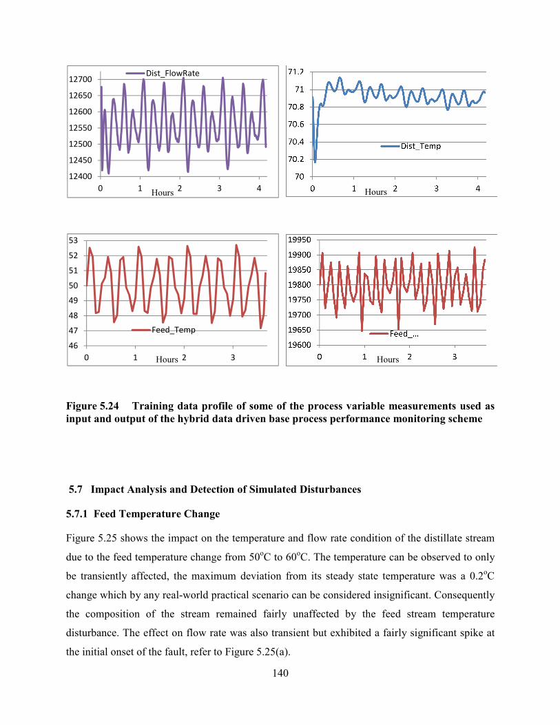
140

Figure 5.24 Training data profile of some of the process variable measurements used as

input and output of the hybrid data driven base process performance monitoring scheme

5.7 Impact Analysis and Detection of Simulated Disturbances

5.7.1 Feed Temperature Change

Figure 5.25 shows the impact on the temperature and flow rate condition of the distillate stream

due to the feed temperature change from 50оC to 60

оC. The temperature can be observed to only

be transiently affected, the maximum deviation from its steady state temperature was a 0.2оC

change which by any real-world practical scenario can be considered insignificant. Consequently

the composition of the stream remained fairly unaffected by the feed stream temperature

disturbance. The effect on flow rate was also transient but exhibited a fairly significant spike at

the initial onset of the fault, refer to Figure 5.25(a).

12400

12450

12500

12550

12600

12650

12700

0 1 2 3 4

Dist_FlowRate

46

47

48

49

50

51

52

53

0 1 2 3

Feed_Temp

Hours Hours

Hours Hours

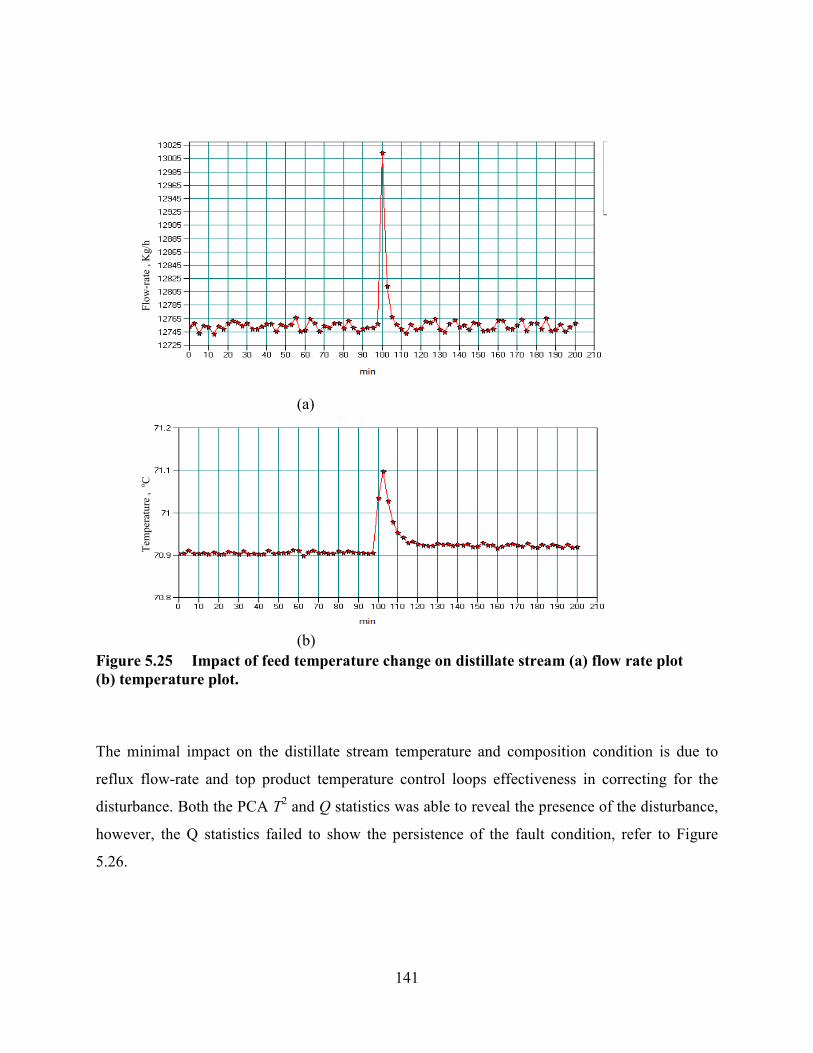
141

Figure 5.25 Impact of feed temperature change on distillate stream (a) flow rate plot

(b) temperature plot.

The minimal impact on the distillate stream temperature and composition condition is due to

reflux flow-rate and top product temperature control loops effectiveness in correcting for the

disturbance. Both the PCA T2 and Q statistics was able to reveal the presence of the disturbance,

however, the Q statistics failed to show the persistence of the fault condition, refer to Figure

5.26.

(a)

(b)

Flo

w-r

ate

, K

g/h

T

emper

atu

re ,

ᴏC

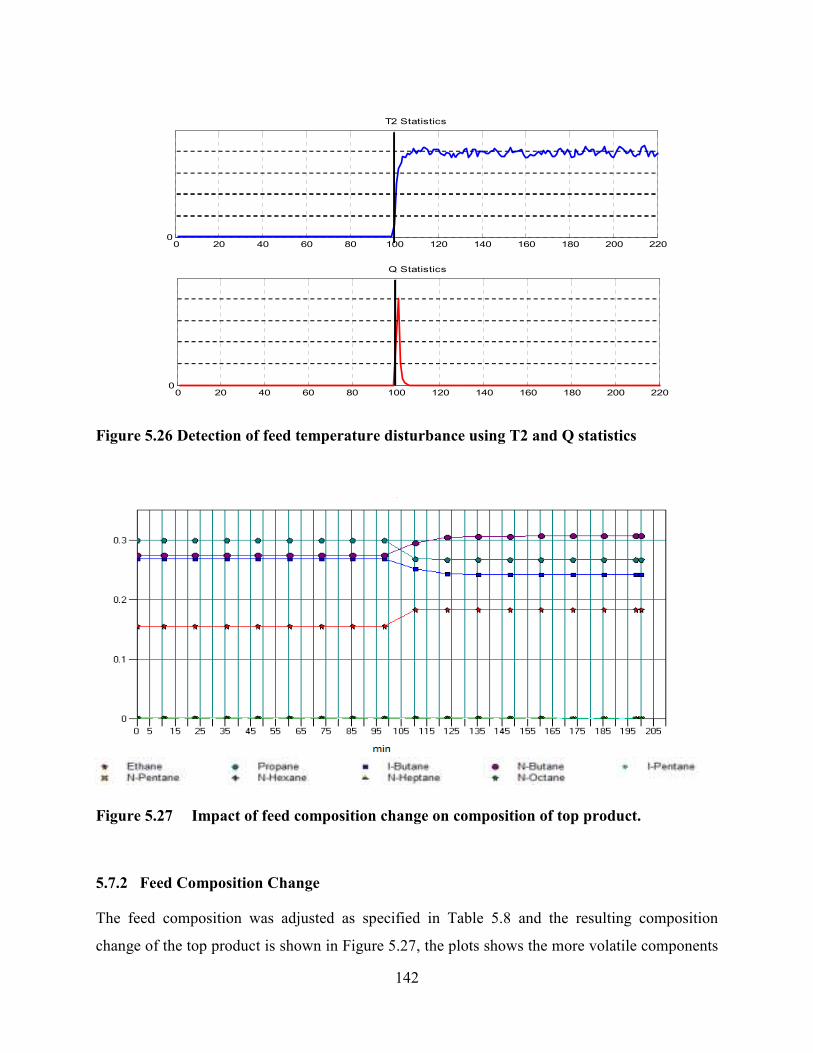
142

Figure 5.26 Detection of feed temperature disturbance using T2 and Q statistics

Figure 5.27 Impact of feed composition change on composition of top product.

5.7.2 Feed Composition Change

The feed composition was adjusted as specified in Table 5.8 and the resulting composition

change of the top product is shown in Figure 5.27, the plots shows the more volatile components

0 20 40 60 80 100 120 140 160 180 200 2200

T2 Statistics

0 20 40 60 80 100 120 140 160 180 200 2200

Q Statistics

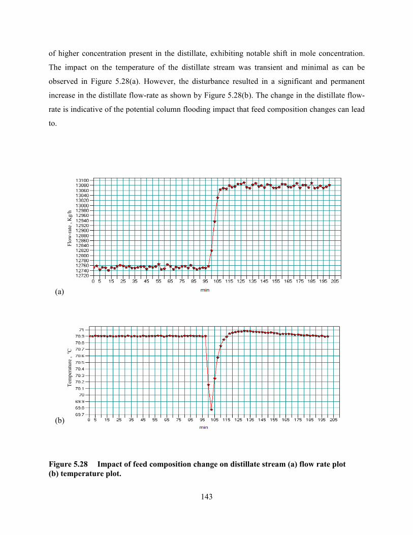
143

of higher concentration present in the distillate, exhibiting notable shift in mole concentration.

The impact on the temperature of the distillate stream was transient and minimal as can be

observed in Figure 5.28(a). However, the disturbance resulted in a significant and permanent

increase in the distillate flow-rate as shown by Figure 5.28(b). The change in the distillate flow-

rate is indicative of the potential column flooding impact that feed composition changes can lead

to.

Figure 5.28 Impact of feed composition change on distillate stream (a) flow rate plot

(b) temperature plot.

(a)

(b)

Flo

w-r

ate

, K

g/h

T

emper

atu

re ,

ᴏC

144

Both the T2 and Q statistics proved effective in detection of the composition disturbance with the

T2 statistics being slightly quicker and aggressive in its detection, see Figure 5.29. Both statistics

also indicate that the fault/disturbance persists.

Figure 5.29 PCA based T2 and Q Statistics detection of composition disturbance.

5.7.3 Change in Feed Flow Rate

The feed flow rate change appears only to have an impact on the distillation stream mass flow

rate variable as shown in Figure 5.30(a), both temperature and composition was unaffected by

the fault. Figure 5.30(b) shows the detection of this disturbance using T2 and Q statistics

computed from applying PCA on the residuals only.

0 10 20 30 40 50 60 70 80 900

T2 Statistics

0 10 20 30 40 50 60 70 80 900

Q Statistics

800

600

400

200

1.0

2.0

3.0

4.0

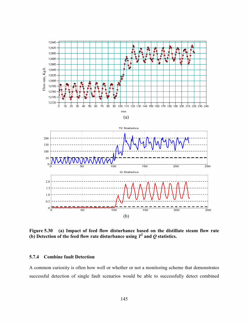
145

Figure 5.30 (a) Impact of feed flow disturbance based on the distillate steam flow rate

(b) Detection of the feed flow rate disturbance using T2 and Q statistics.

5.7.4 Combine fault Detection

A common curiosity is often how well or whether or not a monitoring scheme that demonstrates

successful detection of single fault scenarios would be able to successfully detect combined

0 50 100 150 200 2500

T2 Statistics

0 50 100 150 200 2500

Q Statistics

(a)

(b)

Flo

w r

ate,

Kg/h

0.5

1.0

1.5

2.0

50

100

150

200

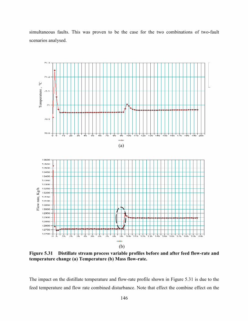
146

simultaneous faults. This was proven to be the case for the two combinations of two-fault

scenarios analysed.

Figure 5.31 Distillate stream process variable profiles before and after feed flow-rate and

temperature change (a) Temperature (b) Mass flow-rate.

The impact on the distillate temperature and flow-rate profile shown in Figure 5.31 is due to the

feed temperature and flow rate combined disturbance. Note that effect the combine effect on the

Flo

w r

ate,

Kg/h

T

emp

erat

ure

,

ᴏC

(a)

(b)

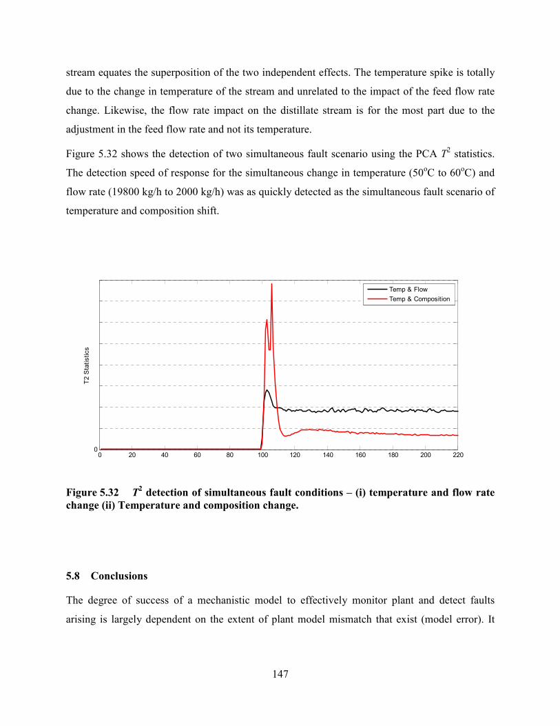
147

stream equates the superposition of the two independent effects. The temperature spike is totally

due to the change in temperature of the stream and unrelated to the impact of the feed flow rate

change. Likewise, the flow rate impact on the distillate stream is for the most part due to the

adjustment in the feed flow rate and not its temperature.

Figure 5.32 shows the detection of two simultaneous fault scenario using the PCA T2 statistics.

The detection speed of response for the simultaneous change in temperature (50оC to 60

оC) and

flow rate (19800 kg/h to 2000 kg/h) was as quickly detected as the simultaneous fault scenario of

temperature and composition shift.

Figure 5.32 T2 detection of simultaneous fault conditions – (i) temperature and flow rate

change (ii) Temperature and composition change.

5.8 Conclusions

The degree of success of a mechanistic model to effectively monitor plant and detect faults

arising is largely dependent on the extent of plant model mismatch that exist (model error). It

0 20 40 60 80 100 120 140 160 180 200 2200

T2 Statistics

Temp & Flow

Temp & Composition

148

was shown that such model parametric errors can lead to offset between the process variables

and plant model output variability and this in some cases inhibits fault detection.

Compensation via linear or non-linear data based model can dramatically improve the fault

detection by providing compensation to correct the inaccuracy of the mechanistic model process

variable estimation. The residual whitening effect of the data based compensation model not only

facilitates fault detection but also improves the reliability of the statistics against false alarm

condition.

A non-mechanistic hybrid approach comprising a NN and OLS model, prove to have the same

degree of success with regards to mitigating false alarm conditions due to shift in processing

operating point and nonlinear process variability. The scheme was also very effective in

detecting the simulated disturbances associated with the column feed stream for both single and

dual simultaneous fault scenarios. In most cases the ability to detect two independent faults

normally translates to being able to detect both faults if occurring simultaneously.

Based upon the analysis study conducted on the impact of several different fault scenarios on the

process variables, one can conclude that a perfect fault diagnosis system capable of automatically

linking a given fault condition to a specific fault scenario case, may not be feasible in all cases.

This being the conclusion as it was observed that for some cases faults of different origins can

affect the same subset of process variables with very similar characteristics. For cases like this a

fault diagnostic system may only be able to narrow the search by identifying a set of possible

fault conditions.

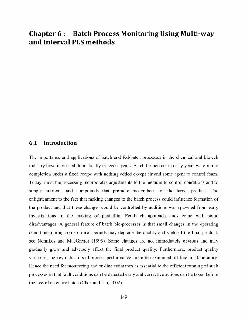
149

Chapter 6 : Batch Process Monitoring Using Multi-way

and Interval PLS methods

6.1 Introduction

The importance and applications of batch and fed-batch processes in the chemical and biotech

industry have increased dramatically in recent years. Batch fermenters in early years were run to

completion under a fixed recipe with nothing added except air and some agent to control foam.

Today, most bioprocessing incorporates adjustments to the medium to control conditions and to

supply nutrients and compounds that promote biosynthesis of the target product. The

enlightenment to the fact that making changes to the batch process could influence formation of

the product and that these changes could be controlled by additions was spawned from early

investigations in the making of penicillin. Fed-batch approach does come with some

disadvantages. A general feature of batch bio-processes is that small changes in the operating

conditions during some critical periods may degrade the quality and yield of the final product,

see Nomikos and MacGregor (1995). Some changes are not immediately obvious and may

gradually grow and adversely affect the final product quality. Furthermore, product quality

variables, the key indicators of process performance, are often examined off-line in a laboratory.

Hence the need for monitoring and on-line estimators is essential to the efficient running of such

processes in that fault conditions can be detected early and corrective actions can be taken before

the loss of an entire batch (Chen and Liu, 2002).

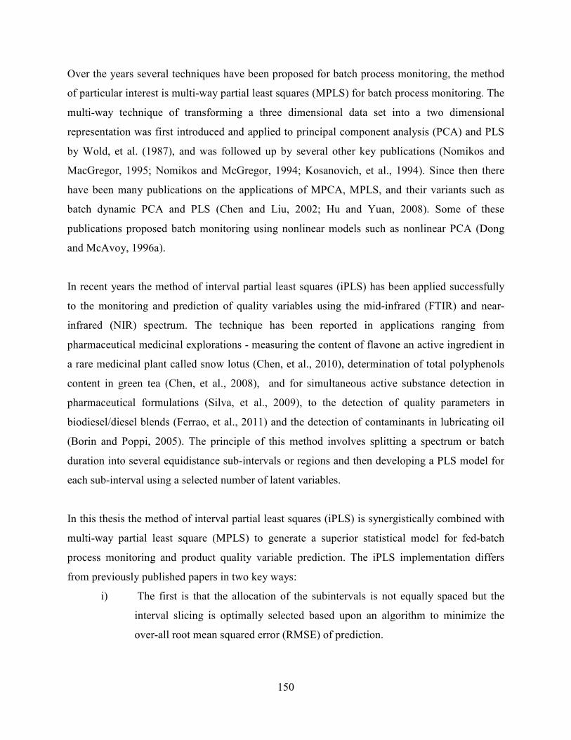
150

Over the years several techniques have been proposed for batch process monitoring, the method

of particular interest is multi-way partial least squares (MPLS) for batch process monitoring. The

multi-way technique of transforming a three dimensional data set into a two dimensional

representation was first introduced and applied to principal component analysis (PCA) and PLS

by Wold, et al. (1987), and was followed up by several other key publications (Nomikos and

MacGregor, 1995; Nomikos and McGregor, 1994; Kosanovich, et al., 1994). Since then there

have been many publications on the applications of MPCA, MPLS, and their variants such as

batch dynamic PCA and PLS (Chen and Liu, 2002; Hu and Yuan, 2008). Some of these

publications proposed batch monitoring using nonlinear models such as nonlinear PCA (Dong

and McAvoy, 1996a).

In recent years the method of interval partial least squares (iPLS) has been applied successfully

to the monitoring and prediction of quality variables using the mid-infrared (FTIR) and near-

infrared (NIR) spectrum. The technique has been reported in applications ranging from

pharmaceutical medicinal explorations - measuring the content of flavone an active ingredient in

a rare medicinal plant called snow lotus (Chen, et al., 2010), determination of total polyphenols

content in green tea (Chen, et al., 2008), and for simultaneous active substance detection in

pharmaceutical formulations (Silva, et al., 2009), to the detection of quality parameters in

biodiesel/diesel blends (Ferrao, et al., 2011) and the detection of contaminants in lubricating oil

(Borin and Poppi, 2005). The principle of this method involves splitting a spectrum or batch

duration into several equidistance sub-intervals or regions and then developing a PLS model for

each sub-interval using a selected number of latent variables.

In this thesis the method of interval partial least squares (iPLS) is synergistically combined with

multi-way partial least square (MPLS) to generate a superior statistical model for fed-batch

process monitoring and product quality variable prediction. The iPLS implementation differs

from previously published papers in two key ways:

i) The first is that the allocation of the subintervals is not equally spaced but the

interval slicing is optimally selected based upon an algorithm to minimize the

over-all root mean squared error (RMSE) of prediction.

151

ii) Secondly, all subintervals are employed as the objective of the model is to support

the detection of fault condition developing at any stage in the batch which may

have adverse impact on the target product quality.

The iPLS model is developed and applied to the batch-wise unfolded data set to produce a Multi-

way iPLS (MiPLS) monitoring and predictive model. The model’s improved fault detection

performance and quality variable prediction capabilities are demonstrated using data generated

from the well-known benchmark fed-batch penicillin fermentation simulator – Pensim (Birol, et

al., 2002). It will also be shown that optimal splitting of the interval can dramatically diminish

the number of subintervals required and subsequently the number of PLS models required to

represent the full spectrum or duration of the batch process.

The chapter is structured as follows. Section 6.2.1 introduces the concept of batch duration

interval splicing and proposes a method of synergistically combining two data unfolding

methods with the interval splicing approach. The novel algorithm proposed by the authors to

achieve optimal interval splicing is described in detail in subsection 6.2.2. Section 6.3 gives a

descriptive overview of the fed-batch penicillin process simulator and provides specifics on the

development of the process monitoring and predictive models employed in this work. Section 6.4

presents simulation results and analysis obtained using the proposed process monitoring and

prediction models. Section 6.5 concludes the paper with a summary of the major conclusions and

findings obtained.

6.2. Combining Data Unfolding and Interval Splicing Techniques

6.2.1 Three-dimensional data unfolding

Multi-way partial least squares MPLS is an extension of PLS to deal with data in three

dimension arrays. MPLS is essentially the equivalent of PLS applied to the unfolded three

dimension data set X (I x J x K) where I is the number of batches J is the number of variables

and K represents the number of measurement samples for the duration of the batch run. As was

shown in Figures 2.4 to 2.6 of chapter 2, the data can be unfolded in one of three different

modes: i) Time ii) Batch and iii) Variable. The approach adopted for this application employed a

merger of both time and batch unfolding methods shown in Figure 6.1.

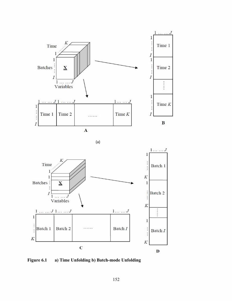
152

(a)

Figure 6.1 a) Time Unfolding b) Batch-mode Unfolding

153

The process involves first splitting the batches along identical time slice intervals. Each

subinterval is then unfolded according to option D in Figure 5.1(b). Data blocks extracted from

identical intervals across each batch are combined into r subinterval grouping and a PLS model

is constructed for each subinterval as shown in Figure 6.2.

Figure 6.2 Batch-wise interval segmented unfolding of data set.

6.2.2 A binary dividing search algorithm approach for subdivision length selection

Critical to the success of this method is the process of arriving at the ideal interval subdivision

across all batches or the selection of a subset of the intervals which will minimize the overall

RMSE. Chen et al. (2010) applied genetic algorithm (GA) programming to select a subset of the

intervals that most efficiently contributes to the prediction of the quality parameter sought to be

quantified. In this subsection we describe a novel procedure which has been effectively applied

to derive the best interval subdivision across all batches. The approach renders the selection of

subintervals unnecessary as it will be demonstrated that if the spectrum or batch duration is

S1

S2

S3

Sr

Batch 1

1

K

S1

S2

S3

Sr

Batch 2

1

K

S1

S2

S3

Sr

Batch I

1

K

1 ……………… J

Batch 1

Batch I

1 …………….. J

Batch 1

Batch I

1 ……………... J

Batch 1

Batch I

Sub-Interval S1: Sub-Interval S2: Sub-Interval Sr:

1 ……………… J 1 ……………… J 1 ……………… J

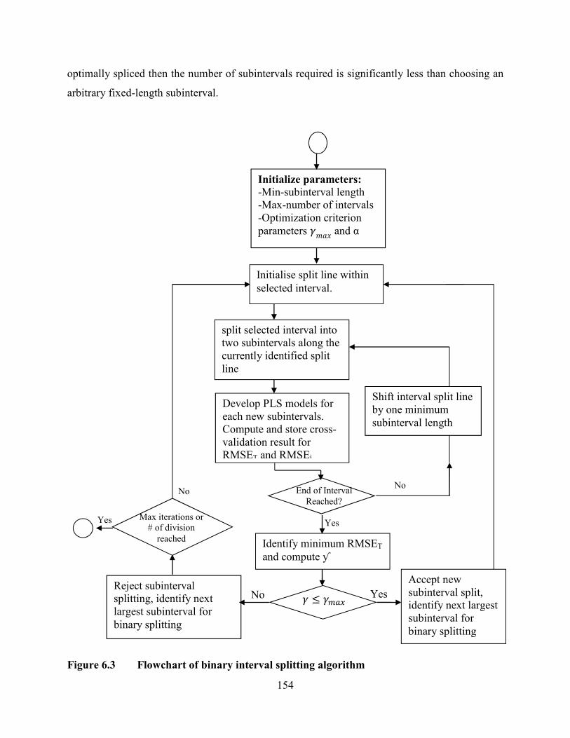
154

optimally spliced then the number of subintervals required is significantly less than choosing an

arbitrary fixed-length subinterval.

Figure 6.3 Flowchart of binary interval splitting algorithm

Initialize parameters:

-Min-subinterval length

-Max-number of intervals

-Optimization criterion

parameters X[� and α

split selected interval into

two subintervals along the

currently identified split

line

Develop PLS models for

each new subintervals.

Compute and store cross-

validation result for

RMSET and RMSEi

Identify minimum RMSET

and compute ƴ

Reject subinterval

splitting, identify next

largest subinterval for

binary splitting

End of Interval

Reached?

X ≤ X@K�

Max iterations or

# of division

reached

No

Yes

Yes No

Yes

No

Accept new

subinterval split,

identify next largest

subinterval for

binary splitting

Shift interval split line

by one minimum

subinterval length

Initialise split line within

selected interval.

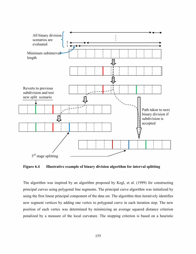
155

Figure 6.4 Illustrative example of binary division algorithm for interval splitting

The algorithm was inspired by an algorithm proposed by Kegl, et al. (1999) for constructing

principal curves using polygonal line segments. The principal curve algorithm was initialized by

using the first linear principal component of the data set. The algorithm then iteratively identifies

new segment vertices by adding one vertex to polygonal curve in each iteration step. The new

position of each vertex was determined by minimizing an average squared distance criterion

penalized by a measure of the local curvature. The stopping criterion is based on a heuristic

Reverts to previous

subdivision and test

new split scenario

Path taken to next

binary division if

subdivision is

accepted

3rd

stage splitting

previous

1 2

All binary division

scenarios are

evaluated

Minimum subinterval

length

156

complexity measure, determined by the number of segments k, the dimension of data matrix, and

the average squared distance of the polygonal line from the data points.

The proposed algorithm is initialized by defining first a minimum subinterval length or step size,

all subsequently selected interval lengths are integer multiples of this minimum interval spacing.

The process could be best described as an iterative binary subdivision process that terminates

when either a predefined maximum number of subdivisions is reached or the algorithm deems

that further subdivision of the intervals would not achieve any significant improvement in the

RMSE of prediction. To evaluate the degree of success or failure of a given subdivision stage,

we define two measurement - the total and segment RMSE, given by Eq. (6.1) and Eq. (6.2)

respectively, note that the total batch RMSE is computed as a weighted sum of the interval

RMSE such that the largest subinterval will have the most influence on the overall value.

�c�=� = Y 6� �c�=/I/d1

(6.1)

�c�=/ = 4Y�Ã�)� J 6

(6.2)

where ni is the length of the ith subinterval, N is the full length of the batch duration and r is the

total number of segments the batch is currently divided into, %Ã is the estimated/predicted value of

the quality variable measurement y based upon the PLS model of the ith subinterval.

Identifying the best binary split of any given segment is a sequential process of evaluating all

split scenarios as illustrated in the flowchart of Figure 6.3 and the example of Figure 6.4. The

partitioning is adjusted in discrete step size defined by the minimum subinterval. The binary

division algorithm compares the segment RMSE value (RMSEi) before a split (�c�=/�)) with

the weighted sum of the RMSE of the split version of the given interval (�c�=/�)) to determine

whether splitting the segment into two parts achieves any improvement over keeping the

segment as a single block. Additionally, the impact of a given subinterval binary splitting on the

157

total RMSE (RMSET) is factored in by considering the ratio of the combined weighted RMSE

across all subintervals before and after the most recent binary split:

X/ = e fgmh�Ufgmh�ç + 1 − e fgmh6Ufgmh6ç

(6.3)

where �c�=�� is the evaluated total RMSE after a given subinterval is trialed split and �c�=��

is the total RMSE before. The weight parameter α takes on values over the range from 0 to 1,

setting the parameter closer to 1 allows more emphasis to be placed on improving the total

RMSE of the fit. By design, therefore, γ will take on values less than 1 if a given trial split of a

subinterval reduces the overall RMSE and will be equal to or greater than 1 if the experimental

splitting of the batch fails to improve the prediction fit.

Based upon the criterion of Eq. (6.3), the algorithm is biased to splitting of the largest subinterval

in any given stage since a registered improvement in the segment RMSE resulting from binary

splitting exercise will impact the RMSET value more if that particular subinterval represents a

larger proportion of the total batch duration. Therefore, as indicated in Figure 6.4, the flow of the

program will first target the largest subinterval and may either revert to the previous state if the

split is rejected or proceed, in either case targeting the next largest subinterval for splitting.

After the optimal subdivision of the batch duration is arrived at, the final stage of the process

involves developing a partial least squares model to fit each interval:

∑∑∑∑====

++++ −−−−====k

i

iik pTXE1

1 and ∑∑∑∑====

++++ −−−−====k

i

iik qUYF1

1

(6.4)

where k is the number of latent variables used to defined a given interval, X is the process

measurements, Y is the process quality variables. The process measurement and quality variable

are therefore simultaneously decomposed into a set of scores T and U using a matrix of loading

vectors p and q, respectively. A linear inner relation between the scores ensures that the scores of

X are generated to be most correlated while being highly predictive of Y.

158

The binary division interval splicing algorithm was first evaluated using simulated data defined

by Eq. (6.5), the coefficients a1 and a2 of the equation were designed to take on different

parameter values over different time interval range. Subsequently, the linear relationship

between the response variable y and predictor variables x1 and x2 is dependent upon the current

time or sample instance. The data is corrupted with random noise of n(t) with zero mean and

variance equal to 10% that of the true measurement variances. Three different scenarios

experimented with are provided in the leftmost column of Table 1.

%Y = [1�1Y + [?�?Y + \Y

(6.5)

Ten batches of data each spanning a batch duration of 300 samples (a matrix of data with the size

3 x 300 for each batch) were generated and the multiway unfolding and interval splitting

algorithm was applied. The final results obtained and the number of iterations used to arrive at

the interval subdivision outcomes are summarized in Table 6.1. The number of stages required in

case was equal to twice the number of subdivision as the algorithm before terminating would

iterates through each discovered subinterval to determine whether further binary splitting was

necessary.

It was found that the algorithm gave best results when the weight parameter α and the value of

γmax were assigned values in the range: 0.6 < α < 1.0 and 0.8 < γmax < 0.9 respectively. If γmax

was chosen too close to the value of 1.0 and or α chosen to be 0.5 or less, the binary division

algorithm was found to be too sensitive to provide improvement in the segment RMSE – RMSEi

and had the tendency of overshooting the actual number of segment intervals required in some

cases. The number of iterations per stage is a function of the minimum subinterval length (Smin)

and the subdivision discovery path taken by the algorithm. Figure 6.5 shows the prediction fitting

evolution for the response variable y as the algorithm discovered the optimal splicing of batch

data set range.

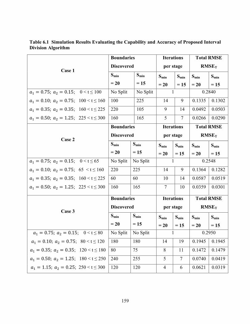
159

Table 6.1 Simulation Results Evaluating the Capability and Accuracy of Proposed Interval

Division Algorithm

Case 1

Boundaries

Discovered

Iterations

per stage

Total RMSE

RMSET

Smin

= 20

Smin

= 15

Smin

= 20

Smin

= 15

Smin

= 20

Smin

= 15 [1 = 0.75; )[? = 0.15 ; 0 < t ≤ 100 [1 = 0.10; )[? = 0.75 ; 100 < t ≤ 160 [1 = 0.35; )[? = 0.35 ; 160 < t ≤ 225 [1 = 0.50; )[? = 1.25 ; 225 < t ≤ 300

No Split No Split 1 0.2840

100 225 14 9 0.1335 0.1302

220 105 9 14 0.0492 0.0503

160 165 5 7 0.0266 0.0290

Case 2

Boundaries

Discovered

Iterations

per stage

Total RMSE

RMSET

Smin

= 20

Smin

= 15

Smin

= 20

Smin

= 15

Smin

= 20

Smin

= 15 [1 = 0.75; )[? = 0.15 ; 0 < t ≤ 65 [1 = 0.10; )[? = 0.75 ; 65 < t ≤ 160 [1 = 0.35; )[? = 0.35 ; 160 < t ≤ 225 [1 = 0.50; )[? = 1.25 ; 225 < t ≤ 300


220 225 14 9 0.1364 0.1282

60 60 10 14 0.0587 0.0519

160 165 7 10 0.0359 0.0301

Case 3

Boundaries

Discovered

Iterations

per stage

Total RMSE

RMSET

Smin

= 20

Smin

= 15

Smin

= 20

Smin

= 15

Smin

= 20

Smin

= 15 [1 = 0.75; )[? = 0.15 ; 0 < t ≤ 80 [1 = 0.10; )[? = 0.75 ; 80 < t ≤ 120 [1 = 0.35; )[? = 0.35 ; 120 < t ≤ 180 [1 = 0.50; )[? = 1.25 ; 180 < t ≤ 250 [1 = 1.15; )[? = 0.25; 250 < t ≤ 300


180 180 14 19 0.1945 0.1945

80 75 8 11 0.1472 0.1479

240 255 5 7 0.0740 0.0419

120 120 4 6 0.0621 0.0319

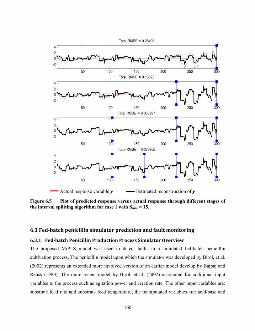
160

Figure 6.5 Plot of predicted response versus actual response through different stages of

the interval splitting algorithm for case 1 with Smin = 15.

6.3 Fed-batch penicillin simulator prediction and fault monitoring

6.3.1 Fed-batch Penicillin Production Process Simulator Overview

The proposed MiPLS model was used to detect faults in a simulated fed-batch penicillin

cultivation process. The penicillin model upon which the simulator was developed by Birol, et al.

(2002) represents an extended more involved version of an earlier model develop by Bajpaj and

Reuss (1980). The more recent model by Birol, et al. (2002) accounted for additional input

variables to the process such as agitation power and aeration rate. The other input variables are:

substrate feed rate and substrate feed temperature; the manipulated variables are: acid/base and

50 100 150 200 250 300

-2

0

2

4

Total RMSE = 0.28403

50 100 150 200 250 300

-2

0

2

4


50 100 150 200 250 300

-2

0

2

4


50 100 150 200 250 300

-2

0

2

4


Actual response variable y Estimated reconstruction of y

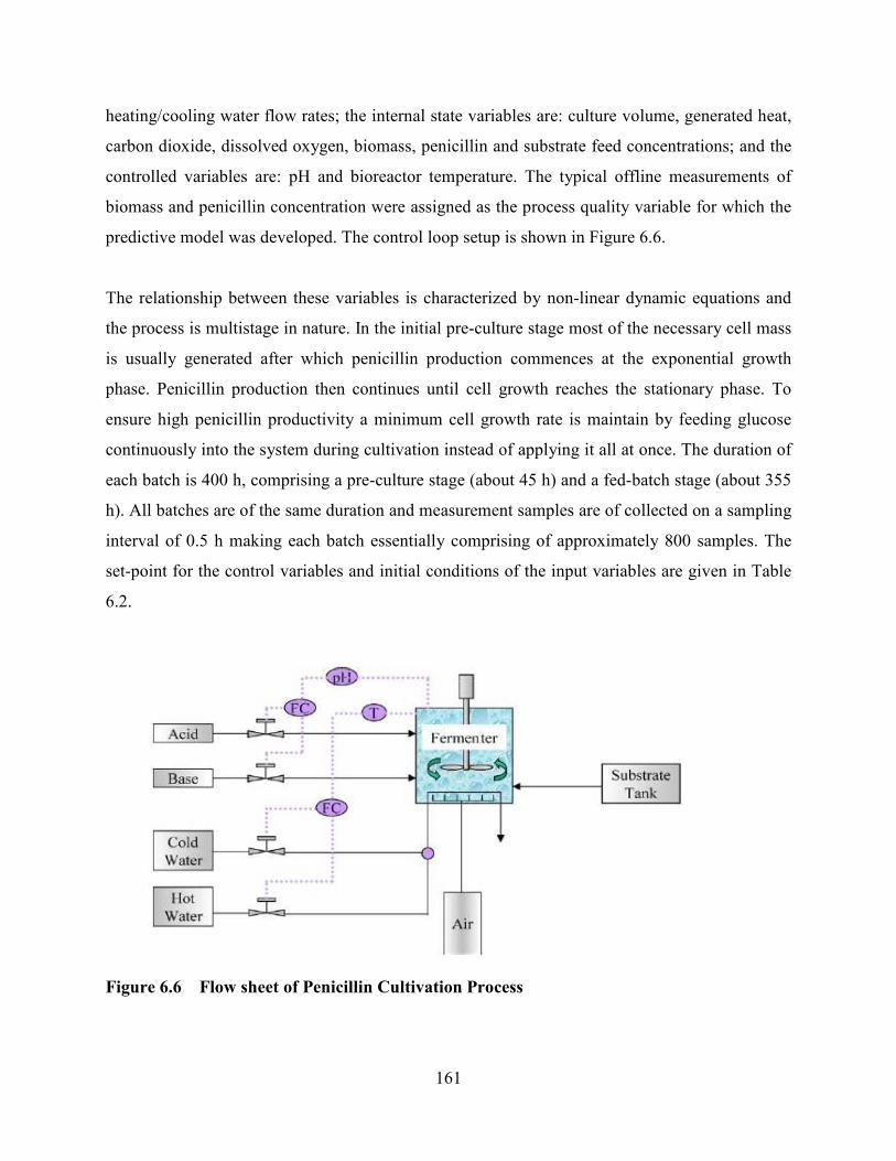
161

heating/cooling water flow rates; the internal state variables are: culture volume, generated heat,

carbon dioxide, dissolved oxygen, biomass, penicillin and substrate feed concentrations; and the

controlled variables are: pH and bioreactor temperature. The typical offline measurements of

biomass and penicillin concentration were assigned as the process quality variable for which the

predictive model was developed. The control loop setup is shown in Figure 6.6.

The relationship between these variables is characterized by non-linear dynamic equations and

the process is multistage in nature. In the initial pre-culture stage most of the necessary cell mass

is usually generated after which penicillin production commences at the exponential growth

phase. Penicillin production then continues until cell growth reaches the stationary phase. To

ensure high penicillin productivity a minimum cell growth rate is maintain by feeding glucose

continuously into the system during cultivation instead of applying it all at once. The duration of

each batch is 400 h, comprising a pre-culture stage (about 45 h) and a fed-batch stage (about 355

h). All batches are of the same duration and measurement samples are of collected on a sampling

interval of 0.5 h making each batch essentially comprising of approximately 800 samples. The

set-point for the control variables and initial conditions of the input variables are given in Table

6.2.

Figure 6.6 Flow sheet of Penicillin Cultivation Process

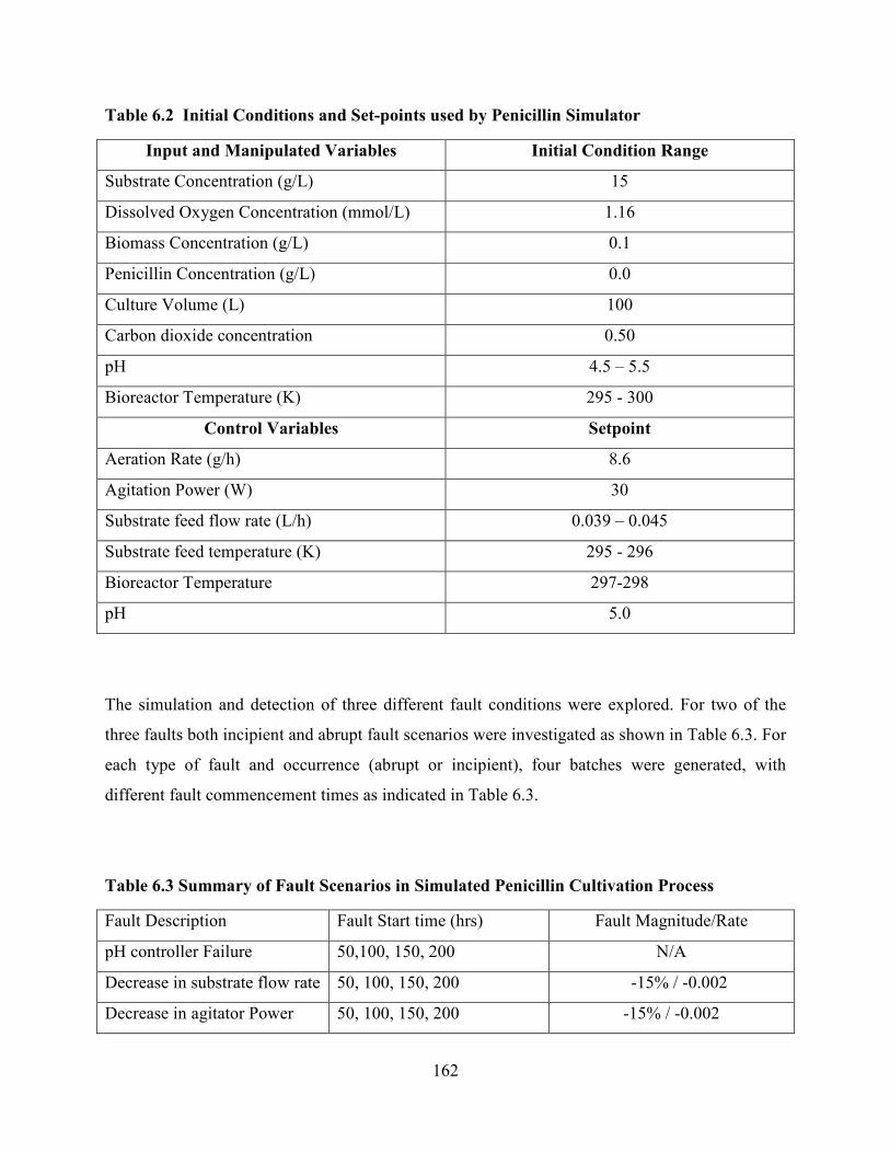
162

Table 6.2 Initial Conditions and Set-points used by Penicillin Simulator

Input and Manipulated Variables Initial Condition Range

Substrate Concentration (g/L) 15

Dissolved Oxygen Concentration (mmol/L) 1.16

Biomass Concentration (g/L) 0.1

Penicillin Concentration (g/L) 0.0

Culture Volume (L) 100

Carbon dioxide concentration 0.50

pH 4.5 – 5.5

Bioreactor Temperature (K) 295 - 300

Control Variables Setpoint

Aeration Rate (g/h) 8.6

Agitation Power (W) 30

Substrate feed flow rate (L/h) 0.039 – 0.045

Substrate feed temperature (K) 295 - 296

Bioreactor Temperature 297-298

pH 5.0

The simulation and detection of three different fault conditions were explored. For two of the

three faults both incipient and abrupt fault scenarios were investigated as shown in Table 6.3. For

each type of fault and occurrence (abrupt or incipient), four batches were generated, with

different fault commencement times as indicated in Table 6.3.

Table 6.3 Summary of Fault Scenarios in Simulated Penicillin Cultivation Process

Fault Description Fault Start time (hrs) Fault Magnitude/Rate

pH controller Failure 50,100, 150, 200 N/A

Decrease in substrate flow rate 50, 100, 150, 200 -15% / -0.002

Decrease in agitator Power 50, 100, 150, 200 -15% / -0.002

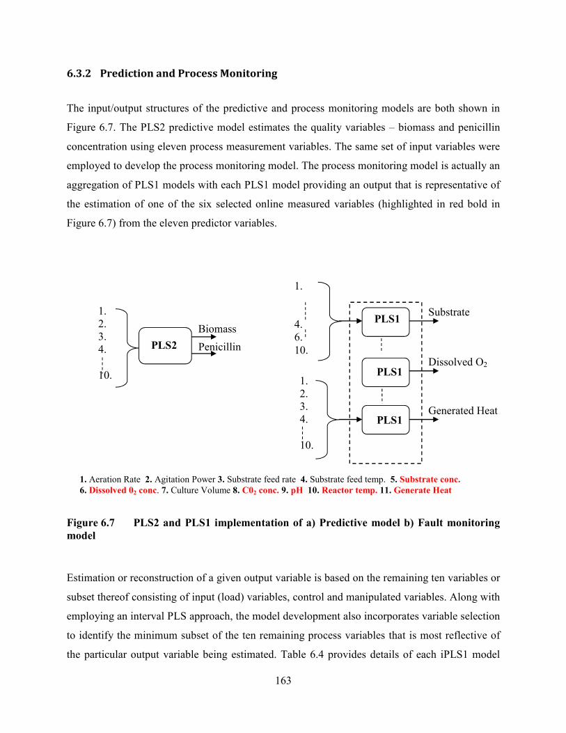
163

6.3.2 Prediction and Process Monitoring

The input/output structures of the predictive and process monitoring models are both shown in

Figure 6.7. The PLS2 predictive model estimates the quality variables – biomass and penicillin

concentration using eleven process measurement variables. The same set of input variables were

employed to develop the process monitoring model. The process monitoring model is actually an

aggregation of PLS1 models with each PLS1 model providing an output that is representative of

the estimation of one of the six selected online measured variables (highlighted in red bold in

Figure 6.7) from the eleven predictor variables.

Figure 6.7 PLS2 and PLS1 implementation of a) Predictive model b) Fault monitoring

model

Estimation or reconstruction of a given output variable is based on the remaining ten variables or

subset thereof consisting of input (load) variables, control and manipulated variables. Along with

employing an interval PLS approach, the model development also incorporates variable selection

to identify the minimum subset of the ten remaining process variables that is most reflective of

the particular output variable being estimated. Table 6.4 provides details of each iPLS1 model

PLS2

PLS1

PLS1

PLS1

1. Aeration Rate 2. Agitation Power 3. Substrate feed rate 4. Substrate feed temp. 5. Substrate conc.

6. Dissolved 02 conc. 7. Culture Volume 8. C02 conc. 9. pH 10. Reactor temp. 11. Generate Heat

1.

2.

3.

4.

10.

Biomass

Penicillin

Substrate

Dissolved O2

Generated Heat

1.

2.

3.

4.

10.

1.

4.

6.

10.

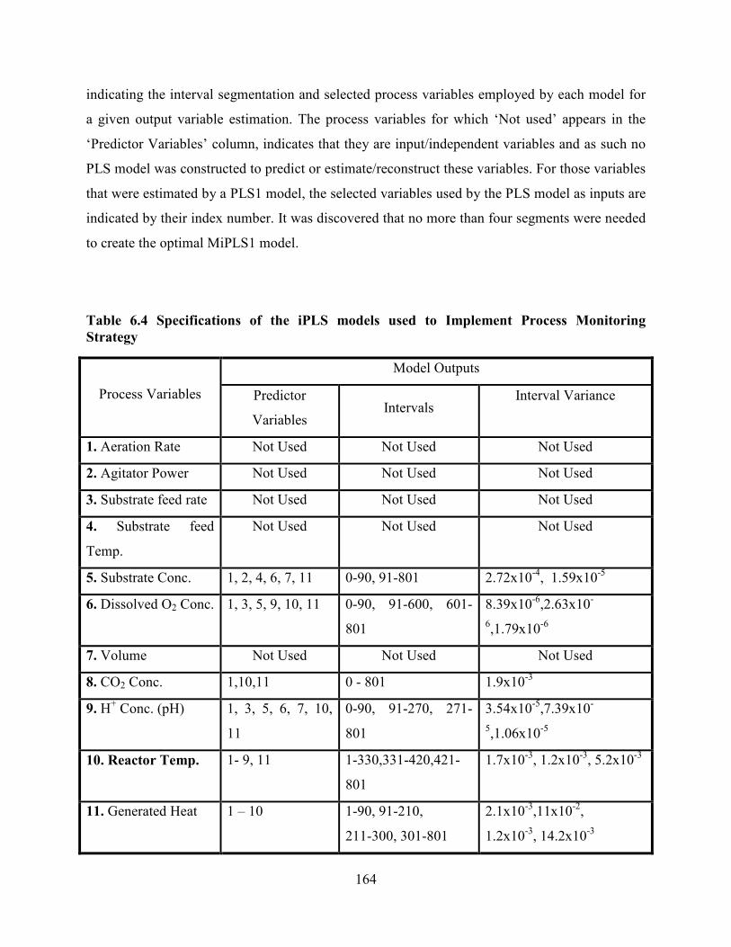
164

indicating the interval segmentation and selected process variables employed by each model for

a given output variable estimation. The process variables for which ‘Not used’ appears in the

‘Predictor Variables’ column, indicates that they are input/independent variables and as such no

PLS model was constructed to predict or estimate/reconstruct these variables. For those variables

that were estimated by a PLS1 model, the selected variables used by the PLS model as inputs are

indicated by their index number. It was discovered that no more than four segments were needed

to create the optimal MiPLS1 model.

Table 6.4 Specifications of the iPLS models used to Implement Process Monitoring

Strategy

Process Variables

Model Outputs

Predictor

Variables Intervals

Interval Variance

1. Aeration Rate Not Used Not Used Not Used

2. Agitator Power Not Used Not Used Not Used

3. Substrate feed rate Not Used Not Used Not Used

4. Substrate feed

Temp.

Not Used Not Used Not Used

5. Substrate Conc. 1, 2, 4, 6, 7, 11 0-90, 91-801 2.72x10-4

, 1.59x10-5

6. Dissolved O2 Conc. 1, 3, 5, 9, 10, 11 0-90, 91-600, 601-

801

8.39x10-6

,2.63x10-

6,1.79x10

-6

7. Volume Not Used Not Used Not Used

8. CO2 Conc. 1,10,11 0 - 801 1.9x10-3

9. H+ Conc. (pH) 1, 3, 5, 6, 7, 10,

11

0-90, 91-270, 271-

801

3.54x10-5

,7.39x10-

5,1.06x10

-5

10. Reactor Temp. 1- 9, 11 1-330,331-420,421-

801

1.7x10-3

, 1.2x10-3

, 5.2x10-3

11. Generated Heat 1 – 10 1-90, 91-210,

211-300, 301-801

2.1x10-3

,11x10-2

,

1.2x10-3

, 14.2x10-3

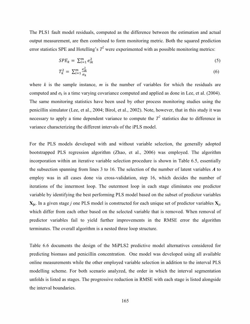
165

The PLS1 fault model residuals, computed as the difference between the estimation and actual

output measurement, are then combined to form monitoring metric. Both the squared prediction

error statistics SPE and Hotelling’s T2 were experimented with as possible monitoring metrics:

�4=^ =)Y ?/?@/d1 (5)

r? =)Y 76kJlk

@/d1 (6)

where k is the sample instance, m is the number of variables for which the residuals are

computed and σk is a time varying covariance computed and applied as done in Lee, et al. (2004).

The same monitoring statistics have been used by other process monitoring studies using the

penicillin simulator (Lee, et al., 2004; Birol, et al., 2002). Note, however, that in this study it was

necessary to apply a time dependent variance to compute the T2 statistics due to difference in

variance characterizing the different intervals of the iPLS model.

For the PLS models developed with and without variable selection, the generally adopted

bootstrapped PLS regression algorithm (Zhao, et al., 2006) was employed. The algorithm

incorporation within an iterative variable selection procedure is shown in Table 6.5, essentially

the subsection spanning from lines 3 to 16. The selection of the number of latent variables A to

employ was in all cases done via cross-validation, step 16, which decides the number of

iterations of the innermost loop. The outermost loop in each stage eliminates one predictor

variable by identifying the best performing PLS model based on the subset of predictor variables

Xjc. In a given stage j one PLS model is constructed for each unique set of predictor variables Xjc

which differ from each other based on the selected variable that is removed. When removal of

predictor variables fail to yield further improvements in the RMSE error the algorithm

terminates. The overall algorithm is a nested three loop structure.

Table 6.6 documents the design of the MiPLS2 predictive model alternatives considered for

predicting biomass and penicillin concentration. One model was developed using all available

online measurements while the other employed variable selection in addition to the interval PLS

modelling scheme. For both scenario analyzed, the order in which the interval segmentation

unfolds is listed as stages. The progressive reduction in RMSE with each stage is listed alongside

the interval boundaries.

166

Table 6.5 Bootstrap PLS algorithm Integrated Within Variable Selection Algorithm

Step 1 Initiate outermost loop iteration to start at first column c = 1; set j = 1;

Step 2 Mean center and scale X and Y;

3 Remove a predictor variable (column c from X) and save the remaining variables as

Xjc,

set E0 = Xjc and F0 = Y and k = 1.

4 Set uk to the first column of Fk-1

5 V^ = 0^�1� _^ _�_^ m

6 scale wk to unit length: V^ = V^ ZV^Z3

7 2^ = 0^�1V^

8 W^ = `^�1� 2^ 2�2^ m

9 scale qk to unit length: W^ = W^ ZW^Z3

10 _a^ = `^�1� W^ W�W^ m

11 Check for convergence. set _^ = _a^

12 If converges go to step 13 else return to step 5

13 Ek-1 loadings: b^ = 0^�1� 2^ 2�2^ 3

14 Regress uk unto tk: c^ = _�2^ 2�2^ 3

15 Compute Residuals:)0^ = 0^ − 2^b� and )`^ = `^ − c^2^b�

16 Apply cross-validation to determine whether to generate additional latent structure if

required then return to step 5 else move to step 17.

17 Execute interval splicing algorithm, repeating steps 3 to 16 to identify optimal

interval splitting; save best iPLS model.

18 If c is less than columns of X then set c = c + 1 and return to step (2) else step 19;

19 Identify best PLS model based on RMSE comparison and set new X = Xjc (best

case);

20 If j > 1 compare current best case PLS model with previous if RMSE if lower then set

j = j + 1 and return step 1 else terminate outermost loop;

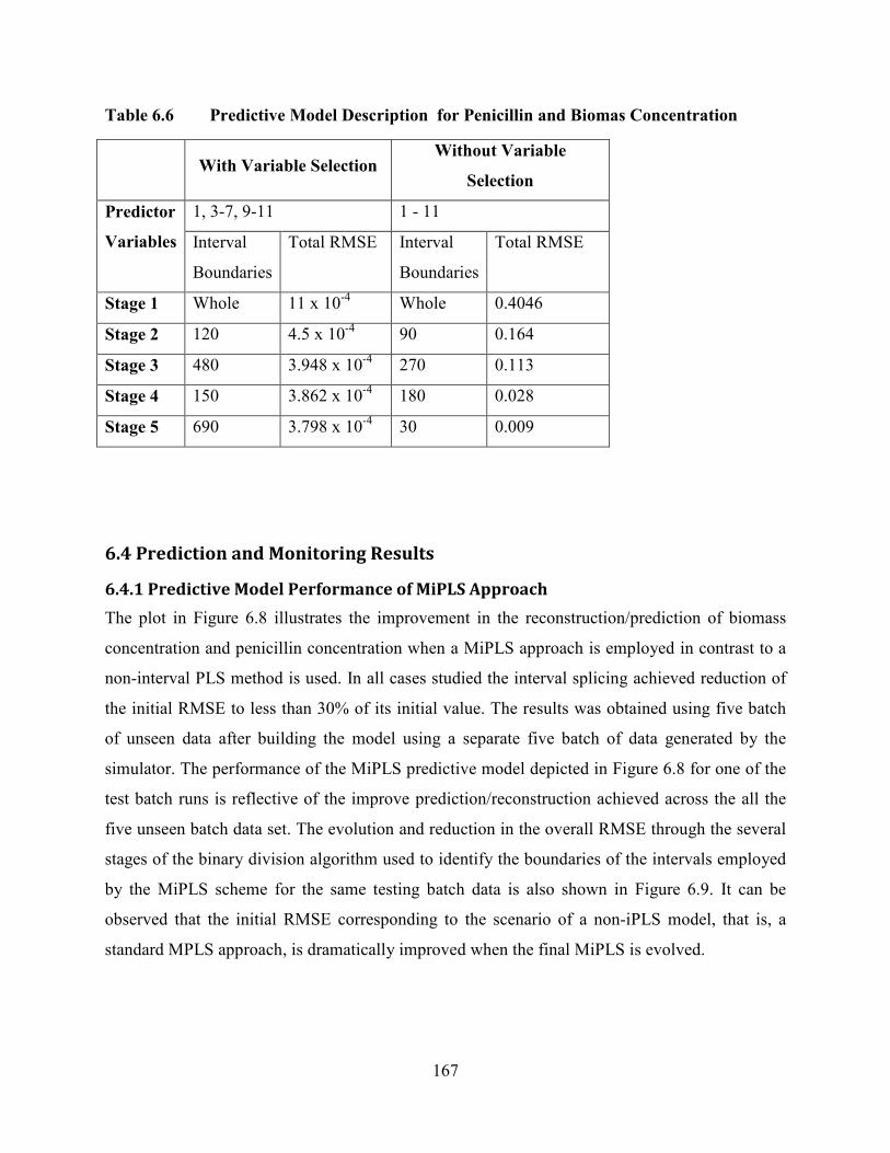
167

Table 6.6 Predictive Model Description for Penicillin and Biomas Concentration

With Variable Selection

Without Variable

Selection

Predictor

Variables

1, 3-7, 9-11 1 - 11

Interval

Boundaries

Total RMSE Interval

Boundaries

Total RMSE

Stage 1 Whole 11 x 10-4

Whole 0.4046

Stage 2 120 4.5 x 10-4 90 0.164

Stage 3 480 3.948 x 10-4 270 0.113

Stage 4 150 3.862 x 10-4 180 0.028

Stage 5 690 3.798 x 10-4

30 0.009

6.4 Prediction and Monitoring Results

6.4.1 Predictive Model Performance of MiPLS Approach

The plot in Figure 6.8 illustrates the improvement in the reconstruction/prediction of biomass

concentration and penicillin concentration when a MiPLS approach is employed in contrast to a

non-interval PLS method is used. In all cases studied the interval splicing achieved reduction of

the initial RMSE to less than 30% of its initial value. The results was obtained using five batch

of unseen data after building the model using a separate five batch of data generated by the

simulator. The performance of the MiPLS predictive model depicted in Figure 6.8 for one of the

test batch runs is reflective of the improve prediction/reconstruction achieved across the all the

five unseen batch data set. The evolution and reduction in the overall RMSE through the several

stages of the binary division algorithm used to identify the boundaries of the intervals employed

by the MiPLS scheme for the same testing batch data is also shown in Figure 6.9. It can be

observed that the initial RMSE corresponding to the scenario of a non-iPLS model, that is, a

standard MPLS approach, is dramatically improved when the final MiPLS is evolved.

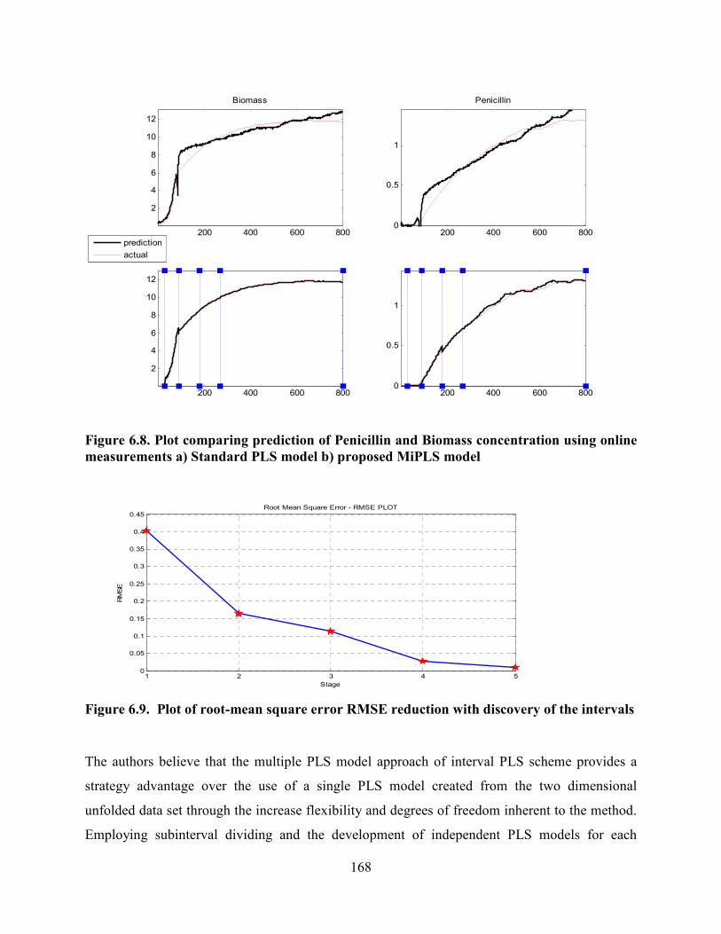
168

Figure 6.8. Plot comparing prediction of Penicillin and Biomass concentration using online

measurements a) Standard PLS model b) proposed MiPLS model

Figure 6.9. Plot of root-mean square error RMSE reduction with discovery of the intervals

The authors believe that the multiple PLS model approach of interval PLS scheme provides a

strategy advantage over the use of a single PLS model created from the two dimensional

unfolded data set through the increase flexibility and degrees of freedom inherent to the method.

Employing subinterval dividing and the development of independent PLS models for each

200 400 600 800

2

4

6

8

10

12

Biomass

200 400 600 8000

0.5

1

Penicillin

200 400 600 800

2

4

6

8

10

12

200 400 600 8000

0.5

1

prediction

actual

1 2 3 4 50

0.05

0.1

0.15

0.2

0.25

0.3

0.35

0.4

0.45Root Mean Square Error - RMSE PLOT

Stage

RMSE

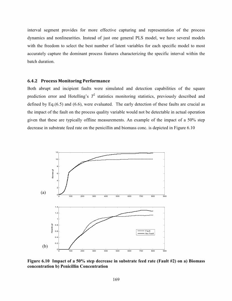
169

interval segment provides for more effective capturing and representation of the process

dynamics and nonlinearities. Instead of just one general PLS model, we have several models

with the freedom to select the best number of latent variables for each specific model to most

accurately capture the dominant process features characterizing the specific interval within the

batch duration.

6.4.2 Process Monitoring Performance

Both abrupt and incipient faults were simulated and detection capabilities of the square

prediction error and Hotelling’s T2 statistics monitoring statistics, previously described and

defined by Eq.(6.5) and (6.6), were evaluated. The early detection of these faults are crucial as

the impact of the fault on the process quality variable would not be detectable in actual operation

given that these are typically offline measurements. An example of the impact of a 50% step

decrease in substrate feed rate on the penicillin and biomass conc. is depicted in Figure 6.10

Figure 6.10 Impact of a 50% step decrease in substrate feed rate (Fault #2) on a) Biomass

concentration b) Penicillin Concentration

0 100 200 300 400 500 600 700 800 9000

2

4

6

8

10

12

Biomass g/l

0 100 200 300 400 500 600 700 800 9000

0.2

0.4

0.6

0.8

1

1.2

1.4

Penicillin g/l

Fault

No Fault

(a)

(b)

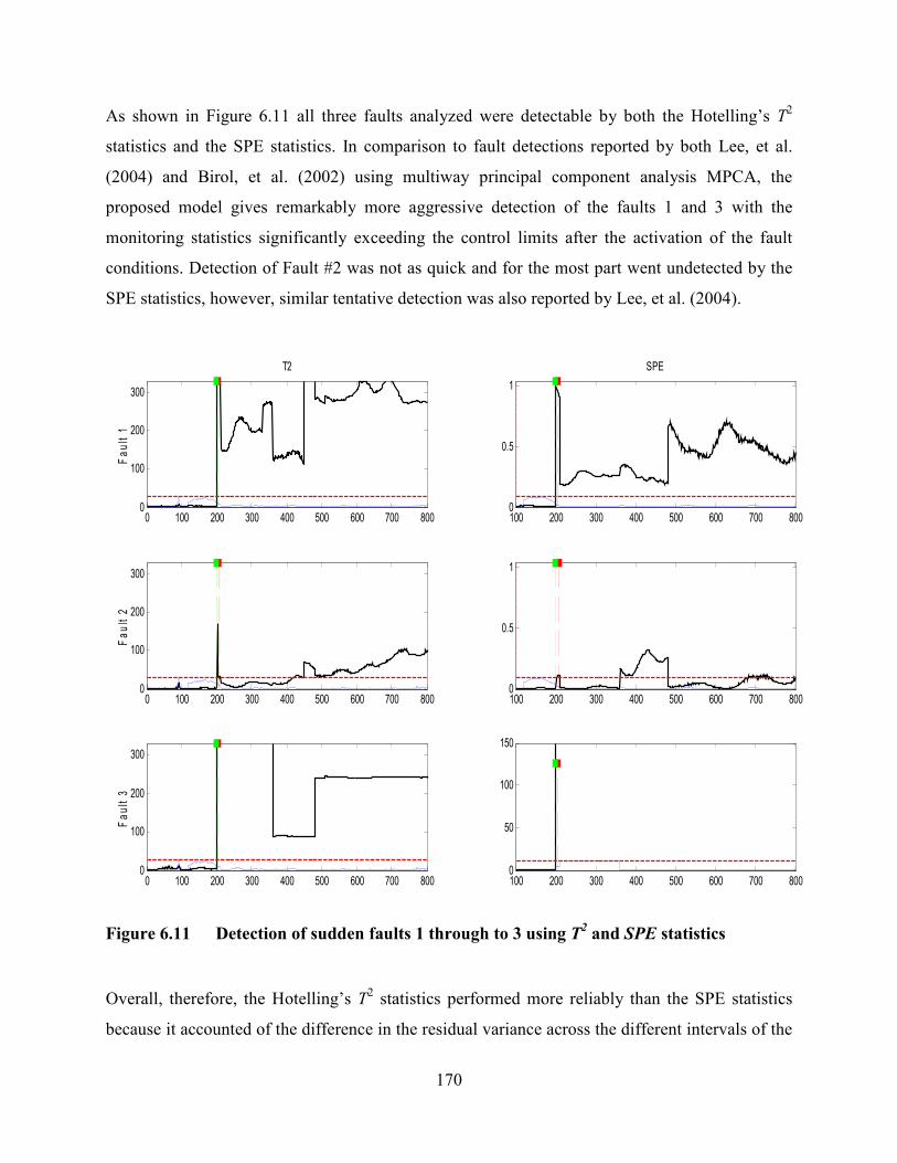
170

As shown in Figure 6.11 all three faults analyzed were detectable by both the Hotelling’s T2

statistics and the SPE statistics. In comparison to fault detections reported by both Lee, et al.

(2004) and Birol, et al. (2002) using multiway principal component analysis MPCA, the

proposed model gives remarkably more aggressive detection of the faults 1 and 3 with the

monitoring statistics significantly exceeding the control limits after the activation of the fault

conditions. Detection of Fault #2 was not as quick and for the most part went undetected by the

SPE statistics, however, similar tentative detection was also reported by Lee, et al. (2004).

Figure 6.11 Detection of sudden faults 1 through to 3 using T2 and SPE statistics

Overall, therefore, the Hotelling’s T2 statistics performed more reliably than the SPE statistics

because it accounted of the difference in the residual variance across the different intervals of the

0 100 200 300 400 500 600 700 8000

100

200

300

T2

Fault 1

100 200 300 400 500 600 700 8000

0.5

1

SPE

0 100 200 300 400 500 600 700 8000

100

200

300

Fault 2

100 200 300 400 500 600 700 8000

0.5

1

0 100 200 300 400 500 600 700 8000

100

200

300

Fault 3

100 200 300 400 500 600 700 8000

50

100

150

171

PLS model fit. To prevent false alarm condition for the SPE statistics it may be advisable to

employ a variable control limit over different interval time span of the batch duration, similar to

the control limits employed by Lee, et al. (2004).

Figure 6.12 compares the incipient fault detection of both fault 1 and 3 for the fault initiation

time of t = 150 hr. The detection of incipient fault # 1 is achieved more readily than incipient

fault # 3.

Figure 6.12 Detection of incipient faults 1 and 2 using Hotelling’s T2 statistics

Figure 6.13 illustrates the detection of an incipient fault (Fault # 2), the point of detection of the

incipient faults and the detection delay time is indicated. For the case of this particular incipient

fault the results indicated a trend of reduce detection delay time for fault initiated later in the

process. For the other two faults simulated the detection delay time was fairly constant.

0 100 200 300 400 500 600 700 8000

50

100

150

200

delay = [223 250]

Normal Operation Fault #1 Fault #2

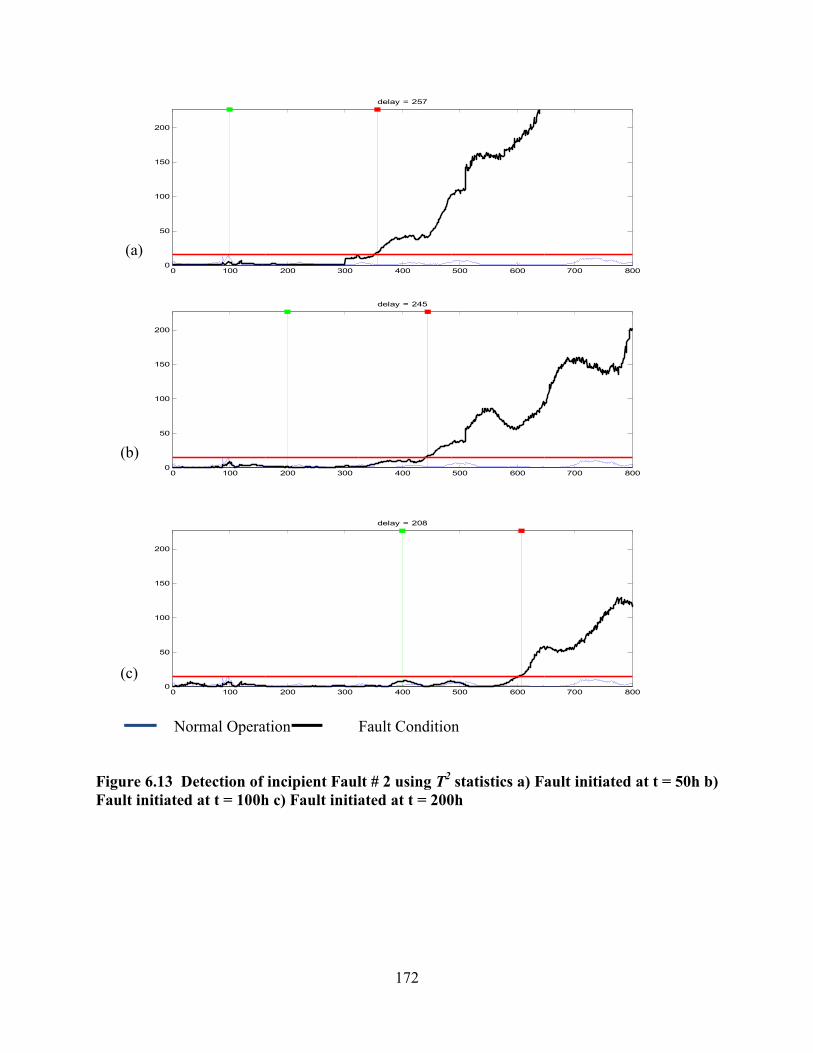
172

Figure 6.13 Detection of incipient Fault # 2 using T2 statistics a) Fault initiated at t = 50h b)

Fault initiated at t = 100h c) Fault initiated at t = 200h

0 100 200 300 400 500 600 700 8000

50

100

150

200

delay = 257

0 100 200 300 400 500 600 700 8000

50

100

150

200

delay = 245

0 100 200 300 400 500 600 700 8000

50

100

150

200

delay = 208

Normal Operation Fault Condition

(b)

(c)

(a)

173

6.5 Conclusion

The predictive capability of the PLS model in terms of quality variables proved to dramatically

improved by combining the interval PLS approach with previously proposed data unfolding

methods. This multi-way modelling approach combined with the proposed algorithm for

identifying the optimal interval subdivision proved to produce significant reduction in the RMSE

over the stand MPLS approach. The binary division algorithms offers an efficient alternative to

employing a fix size interval selection approach to the implementation of an iPLS model. Fix-

interval length iPLS approach would typically involve the use of a genetic algorithm to select a

subset of the intervals that are best predictive of the quality variable. However, the binary

algorithm demonstrates that optimal selection can significantly reduce the number of

segments/intervals needed and thereby eliminating the need for employing a genetic algorithm.

The fault monitoring capabilities of the proposed process monitoring scheme did not provided as

dramatic an improvement in comparison to previously reported methods but demonstrated that it

was just as effective. If more simulated fault scenarios were supported by the simulator, perhaps

a more clear distinction in the fault detection capabilities of the proposed scheme could be

arrived at. Overall, both the Hotelling T2 and SPE statistics seem to be capable of detecting both

incipient and sudden faults arising at the differing points in the cultivation batch process, with

the T2 statistics proving slightly more reliable than the SPE statistics.

174

Chapter 7 : Conclusions and Suggestions for Further

Works

7.1 Conclusions Research efforts in the field of process performance monitoring have had significant impact on

the utilisation of process measurement data gathered from plants. The reported applications have

ranged from quality variable prediction, fault and disturbance detection, knowledge based fault

diagnostic systems, and model based process control systems. Researchers have drawn upon

statistical methods, mathematics, and design concepts from non-chemical engineering disciplines

and adapted, investigate suitability, and conducted comparative study towards the goal of

refining and improving their applicability to field of process performance monitoring. Chapters 2

and 3 reviewed some of these methods, the innovations and improvements have been contributed

over the years by different researchers since the inception of multivariate statistical process

controls.

This thesis also seeks to contribute to the efforts of refining and improving existing methods and

suggest innovative solutions to expand the scope of applicability to more complex processes.

Hence, the main aims and objectives of the thesis as were set out in Chapter 1.

175

The contribution of Chapter 4 sought to satisfy the first stated objective of subsection 1.2 in

Chapter 1. A simplified CVA based state-space model design for the specific purpose of process

monitoring was achieved by way of proposing the use of simpler state space representation more

suitable for process monitoring specific applications and deriving a more efficiently estimation

procedure for parameterization of state space matrices.

The CVA state space model was evaluated on the well-known Tennessee Eastman benchmark

process. The fault detection performance showed that the performance capability of the state

space model was maintained while achieving dramatic simplification of the set of stochastic

estimation equations used to derive the reduce set of model parameters. A comparative study

conducted by comparing published fault detection performance results of other statistical

methods (CA, PCA, DPCA, and the traditionally CVA approach) for the same simulated faults

on TE simulator, revealed that the proposed state space representation gave comparable, and in

many cases better, fault detection performance than the traditional CVA state space modelling

technique. Most notable is the detection of fault No. 15 in the Tennessee Eastman benchmark

process and the significant reduction in detection delay time achieved for the more difficult to

detect faults. The overall best performing monitoring statistics in terms of fault detection and

detection delay time is the Hotelling’s T2 statistics of the output residuals T

2ey.

The fault detection performance also faired comparably to that reported for the DICA and SSICA

schemes (Odiowei and Cao 2010). They reported detection of faults # 3 and 9 a feat not

previously accomplished to the author’s best knowledge. The proposed CVA method,

nevertheless, did fair better in terms of the percentage performance reliability for the faults

detectable.

Chapter 5 explored two hybrid model approaches. One approach considered the merging of a

mechanistic and data driven model based approach. The other investigated a hybrid

implementation of two data based model a NN model and an OLS model. The hybrid

mechanistic data based approaches were evaluated using a CSTR simulator while the hybrid data

based model was evaluated using a ChemCad distillation column simulator.

176

In the case of the proposed mechanistic-data based hybrid scheme, a central difference to that of

the traditional approach was related to the interface between the mechanistic model and the

plant. The proposed scheme suggested using the controller output as injected inputs into the

mechanistic model as oppose to implement the control loop and controller within the model.

Several hybrid variants were evaluated with all demonstrating improve detection performance

over the pure mechanistic approach. It was demonstrated through select fault examples why the

model uncertainty (model plant mismatches) can have negative impact on the fault detection

capability via monitoring of the mechanistic model-plant residuals. The best performing hybrid

model in relation to fault detection was the mechanistic – PLS1 based data based model HM3.

The HM3 data based model was a one step ahead predictive model employing past output

measurements to estimate the current outputs of the data based model.

Sixteen of the eighteen faults simulated on the CSTR were successfully detected, the valve

sticking faults proved undetectable under steady state operation. The collection of detectable

faults included incipient sensor fault drift error faults, the gradual failing of unit operations such

as heat exchanger fouling and pump pressure lost. The impact of the sensor or unit operation

fault was dependent upon whether the unit was incorporated within a control loop or not. Fault

sensors or unit operations within the control or recycle loops could prove more troubling to

isolate because of the inherent propagating effect of the loop.

Both the hybrid data based method proposed in Chapter 5 for the monitoring of the continuous

distillation column and the multi-way interval PLS (MiPLS) model proposed in Chapter 6 for the

monitoring of the batch penicillin process, employed an approach of developing multiple linear

models to approximate and capture the nonlinearity of the process under monitor. The hybrid

approach used OLS regression models to capture the variability in the process data

measurements about different operating feed condition of the stream. The existing steady state

condition of the distillation process was identified by applying a short-term moving average filter

to the past values of the process variables. A NN model successfully provided a means of

switching in the best fit OLS regression model to track and predict the process output variance

based upon the current input variable variance.

177

The MiPLS model, on the other hand, exploited the fix time duration of the batch and derived

linear PLS models that gave the best approximation over the specific interval of the batch. The

optimal interval segmentations were identified by a proposed algorithm inspired by the polygon

line segment algorithm proposed by Kegl et al. (1999) for constructing principal curves. The

accuracy of the prediction of the process quality variables demonstrated significant improvement

when the interval PLS derived using the optimal interval subdivision algorithm was combined

with previously proposed data unfolding methods.

The proposed binary division algorithms offers an efficient alternative to employing a fix size

interval selection approach to the implementation of an iPLS model. Fix-interval length iPLS

approach would typically involve the use of a genetic algorithm to select a subset of the intervals

that are best predictive of the quality variable. Employing the binary algorithm have facilitated

the use of a far smaller set of define segments/intervals to implement the iPLS model thereby

eliminating the need for employing a genetic algorithm.

Investigation into the detection of combine faults conducted in chapter 5 seem to reveal that a

monitoring scheme ability to detect independent single fault conditions usually translates into

being able to detect the existence of a multiple simultaneous fault scenario. The research analysis

was limited two fault scenarios as such no conclusions or comment on multiple simultaneous

faults beyond the two fault scenario can be made.

Building localized fault monitoring systems around specific unit operations or area of a plant

may be more efficient that a plant-wide strategy. The impact of a fault tends to affect variables

local to its vicinity first and may propagate outward, however, earliest detection would therefore

best be facilitated via monitoring of those local variables. A distributed plant monitoring strategy

as opposed to a centralized strategy would also better facilitate fault isolation and diagnostics.

7.2 Suggestions for Further Works A significant amount of the analysis conducted in Chapter 5 was devoted to identify the best

hybrid architecture in terms of mechanistic model – plant interface and the choice of past time

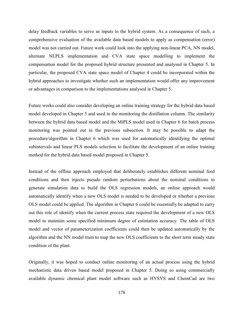
178

delay feedback variables to serve as inputs to the hybrid system. As a consequence of such, a

comprehensive evaluation of the available data based models to apply as compensation (error)

model was not carried out. Future work could look into the applying non-linear PCA, NN model,

alternate NLPLS implementation and CVA state space modelling to implement the

compensation model for the proposed hybrid structure presented and analysed in Chapter 5. In

particular, the proposed CVA state space model of Chapter 4 could be incorporated within the

hybrid approaches to investigate whether such an implementation would offer any improvement

or advantages in comparison to the implementations analysed in Chapter 5.

Future works could also consider developing an online training strategy for the hybrid data based

model developed in Chapter 5 and used to the monitoring the distillation column. The similarity

between the hybrid data based model and the MiPLS model used in Chapter 6 for batch process

monitoring was pointed out in the previous subsection. It may be possible to adapt the

procedure/algorithm in Chapter 6 which was used for automatically identifying the optimal

subintervals and linear PLS models selection to facilitate the development of an online training

method for the hybrid data based model proposed in Chapter 5.

Instead of the offline approach employed that deliberately establishes different nominal feed

conditions and then injects pseudo random perturbations about the nominal conditions to

generate simulation data to build the OLS regression models, an online approach would

automatically identify when a new OLS model is needed to be developed or whether a previous

OLS model could be applied. The algorithm in Chapter 6 could be essentially be adapted to carry

out this role of identify when the current process state required the development of a new OLS

model to maintain some specified minimum degree of estimation accuracy. The table of OLS

model and vector of parameterization coefficients could then be updated automatically by the

algorithm and the NN model train to map the new OLS coefficients to the short term steady state

condition of the plant.

Originally, it was hoped to conduct online monitoring of an actual process using the hybrid

mechanistic data driven based model proposed in Chapter 5. Doing so using commercially

available dynamic chemical plant model software such as HYSYS and ChemCad are two

179

software options readily available if the tradition mechanistic model plant interface is to be

applied. Doing so for the case of the proposed mechanistic model plant interface would however

require some adaptation of the software plant simulator to be able to accept external controller

output signals to drive the plant actuators directly instead of implementing the controller and

control loop within the simulator. In the case of HYSYS this could possibly be achieved by

switching the controllers to manual model and using a spreadsheet to tie the manual output value

of the controllers in the simulator to the actual controller output levels extracted from the plant

SCADA system. In manual mode the controller output can be directly manipulated.

A final proposed area of future work is the use of variable specific lags/leads specification as

opposed to specifying a fix lag/lead window size for all process variables employed by the

dynamic model. Preliminary work and investigation into this design consideration, not

documented in this thesis, does not seem to provide any significant improvement to the dynamic

model developed. However, a more comprehensive investigation may confirm the assertion that

the use of variable specific lag order may facilitate a more effective capturing of the dynamics of

the process variables which may be characterized by different dynamics. One may want to

consider the use of genetic algorithm (GA) to naturally evolve to an optimal or sub optimal

variable lag order selection. This could be combined with the proposed CVA state space model

of Chapter 5 to further improve on the model dimensionality reduction and one-step ahead

prediction accuracy.

180

Appendix A

Introduction

The appendix provides a summary overview of some of the essential coding developed and used

over the duration of my research to carry out model development, simulate and conduct fault

analysis scenarios. Due to size constraints copying the codes directly into the appendix, as was

done with the PLS algorithms at the end of section, would have made the report very bulky and

the appendix not very reader friendly. Consequently, three charts are provided in the appendix to

assist with navigating through some of the scripts/codes archived on the CD attached to the back

of the inside cover of the booklet.

The charts graphically lay out the interlinking between the various scripts, identifying the main

script and various subroutines/called functions employed by each script. The tier structure of the

chart also seeks to indicate the function calling structure, that is, which scripts/functions serve as

subroutines to which other functions.

CVA State Space Model Code

The chart shown in Figure A.1 outlines the code implementation used to conduct significant

components of the analysis and results generated in chapter 4. The state space model

implementation, in particular, was implemented using the script CVASSModel.m which calls

upon three other subroutines as shown in the chart. The other subroutine were used to implement

the monitoring statistics, evaluate fault detection points and carry out various data scaling and

other pre-conditioning operation of the data set.

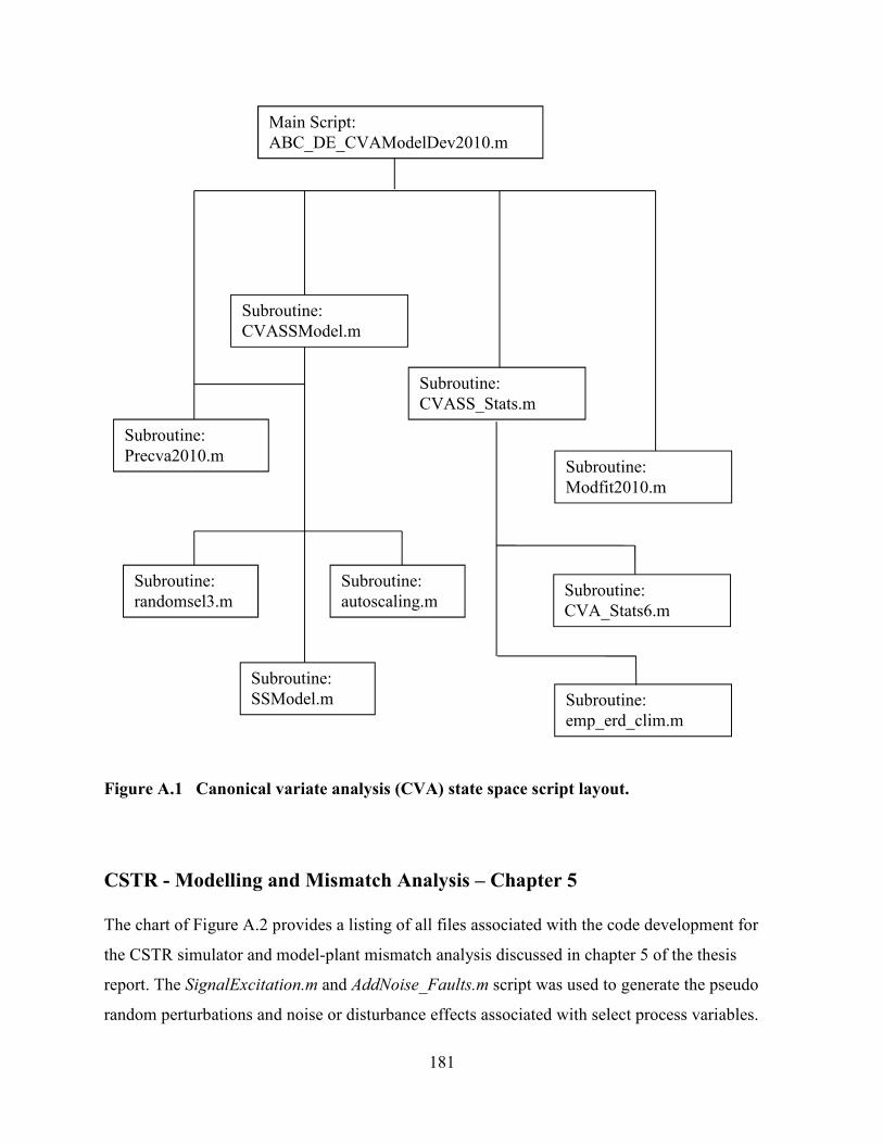
181

Figure A.1 Canonical variate analysis (CVA) state space script layout.

CSTR - Modelling and Mismatch Analysis – Chapter 5

The chart of Figure A.2 provides a listing of all files associated with the code development for

the CSTR simulator and model-plant mismatch analysis discussed in chapter 5 of the thesis

report. The SignalExcitation.m and AddNoise_Faults.m script was used to generate the pseudo

random perturbations and noise or disturbance effects associated with select process variables.

Main Script:

ABC_DE_CVAModelDev2010.m

Subroutine:

Precva2010.m

Subroutine:

CVASSModel.m

Subroutine:

CVASS_Stats.m

Subroutine:

randomsel3.m

Subroutine:

Modfit2010.m

Subroutine:

emp_erd_clim.m

Subroutine:

CVA_Stats6.m

Subroutine:

autoscaling.m

Subroutine:

SSModel.m

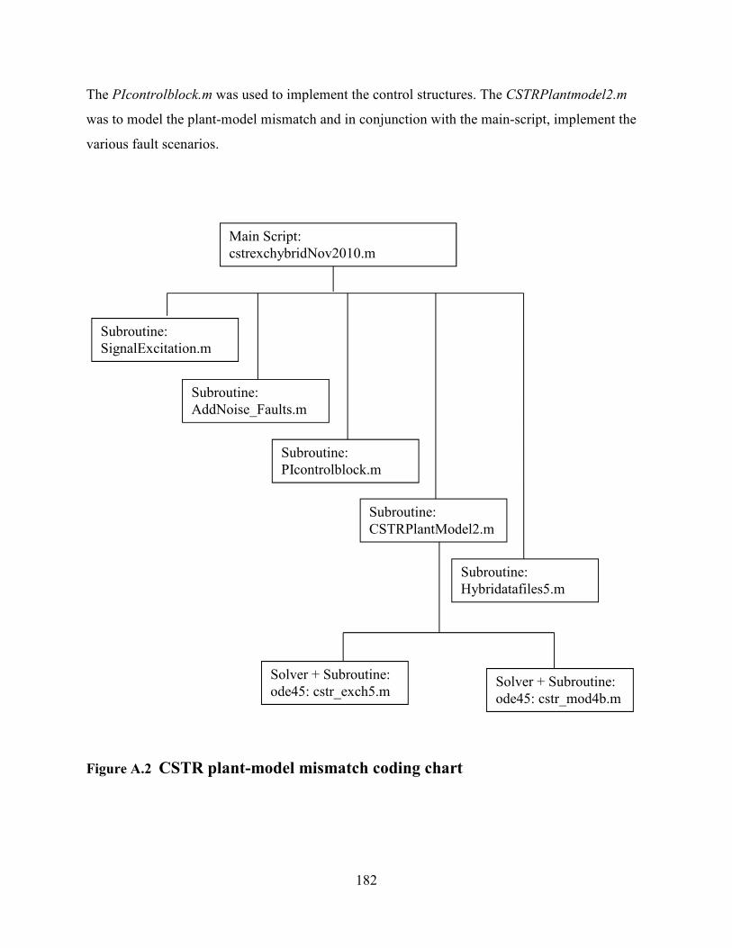
182

The PIcontrolblock.m was used to implement the control structures. The CSTRPlantmodel2.m

was to model the plant-model mismatch and in conjunction with the main-script, implement the

various fault scenarios.

Figure A.2 CSTR plant-model mismatch coding chart

Main Script:

cstrexchybridNov2010.m

Subroutine:

SignalExcitation.m

Subroutine:

AddNoise_Faults.m

Subroutine:

PIcontrolblock.m

Subroutine:

CSTRPlantModel2.m

Subroutine:

Hybridatafiles5.m

Solver + Subroutine:

ode45: cstr_exch5.m Solver + Subroutine:

ode45: cstr_mod4b.m

183

Binary Division Search Algorithm and PLS Algorithms

The chart of Figure A.3 shows the interlink between the matlab script files used to implement the

binary division search algorithm proposed in chapter 6. The segment splitting algorithm can be

adapted to incorporate any regression algorithm or subspace based algorithm for segment

modelling: ordinary least squares OLS, partial least squares PLS, CVA state space modelling,

etc. The loop iterations is implemented in the main script and terminates when the optimal sub-

division splitting and models are derived. The splitsegment2.m script is essential to evaluating a

particular subdivision selection and is an essential and permanent subroutine irregardless of the

regression method employed for segment modelling.

Figure A.3 Code Chart Outline of binary dividing segment length search algorithm

Main Script:

binearysearch_psimfault270111.m

Subroutine:

iOLSxval.m

Subroutine:

multiOLS2.m

Subroutine:

splitsegment2.m

Subroutine:

iOLSxval2.m

Subroutine:

iOLS2.m

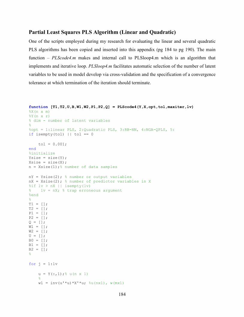
184

Partial Least Squares PLS Algorithm (Linear and Quadratic)

One of the scripts employed during my research for evaluating the linear and several quadratic

PLS algorithms has been copied and inserted into this appendix (pg 184 to pg 190). The main

function – PLScode4.m makes and internal call to PLSloop4.m which is an algorithm that

implements and iterative loop. PLSloop4.m facilitates automatic selection of the number of latent

variables to be used in model develop via cross-validation and the specification of a convergence

tolerance at which termination of the iteration should terminate.

function [T1,T2,U,B,W1,W2,P1,P2,Q] = PLScode4(Y,X,opt,tol,maxiter,lv) %X(n x m) %Y(n x r) % dim - number of latent variables % %opt = 1:linear PLS, 2:Quadratic PLS, 3:RB-NN, 4:NGA-QPLS, 5: if isempty(tol) || tol == 0

tol = 0.001; end %initialize Ysize = size(Y); Xsize = size(X); n = Xsize(1);% number of data samples

nY = Ysize(2); % number or output variables nX = Xsize(2); % number of predictor variables in X %if lv > nX || isempty(lv) % lv = nX; % trap erroneous argument %end % T1 = []; T2 = []; P1 = []; P2 = []; Q = []; W1 = []; W2 = []; U = []; B0 = []; B1 = []; B2 = []; %

for j = 1:lv

u = Y(:,1);% u(n x 1) % w1 = inv(u'*u)*X'*u; %u(nx1), w(mx1)

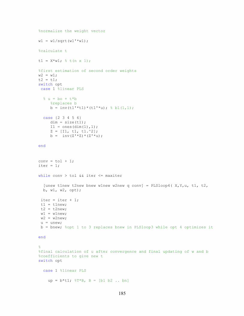
185

%normalize the weight vector

w1 = w1/sqrt(w1'*w1);

%calculate t

t1 = X*w1; % t(n x 1);

%first estimation of second order weights w2 = w1; t2 = t1; switch opt case 1 %linear PLS

% u = bo + t*b %replaces b b = inv(t1'*t1)*(t1'*u); % b1(1,1);

case {2 3 4 5 6} dim = size(t1); I1 = ones(dim(1),1); Z = [I1, t1, t1.^2]; b = inv(Z'*Z)*(Z'*u);

end

conv = tol + 1; iter = 1;

while conv > tol && iter <= maxiter

[unew t1new t2new bnew w1new w2new q conv] = PLSloop4( X,Y,u, t1, t2,

b, w1, w2, opt);

iter = iter + 1; t1 = t1new; t2 = t2new; w1 = w1new; w2 = w2new; u = unew; b = bnew; %opt 1 to 3 replaces bnew in PLSloop3 while opt 4 optimizes it

end

% %final calculation of u after convergence and final updating of w and b %coefficients to give new t switch opt

case 1 %linear PLS

up = b*t1; %T*B, B = [b1 b2 .. bn]

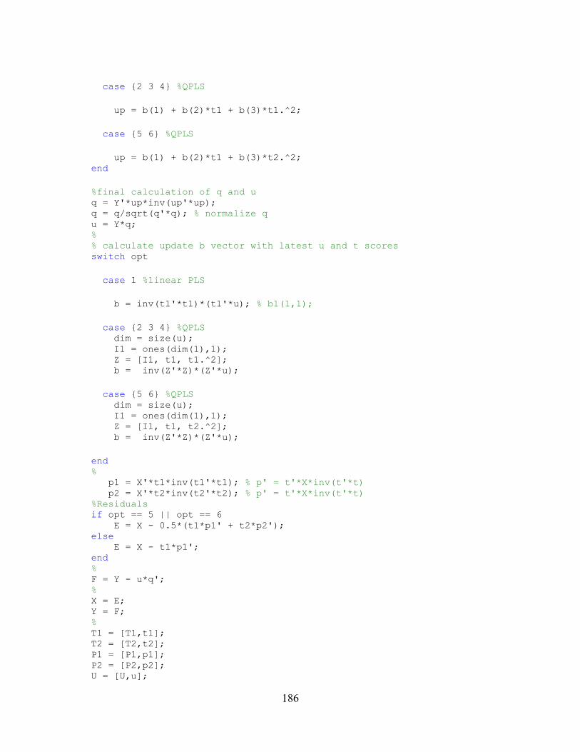
186

case {2 3 4} %QPLS

up = b(1) + b(2)*t1 + b(3)*t1.^2;

case {5 6} %QPLS

up = b(1) + b(2)*t1 + b(3)*t2.^2; end

%final calculation of q and u q = Y'*up*inv(up'*up); q = q/sqrt(q'*q); % normalize q u = Y*q; % % calculate update b vector with latest u and t scores switch opt

case 1 %linear PLS

b = inv(t1'*t1)*(t1'*u); % b1(1,1);

case {2 3 4} %QPLS dim = size(u); I1 = ones(dim(1),1); Z = [I1, t1, t1.^2]; b = inv(Z'*Z)*(Z'*u);

case {5 6} %QPLS dim = size(u); I1 = ones(dim(1),1); Z = [I1, t1, t2.^2]; b = inv(Z'*Z)*(Z'*u);

end % p1 = X'*t1*inv(t1'*t1); % p' = t'*X*inv(t'*t) p2 = X'*t2*inv(t2'*t2); % p' = t'*X*inv(t'*t) %Residuals if opt == 5 || opt == 6 E = X - 0.5*(t1*p1' + t2*p2'); else E = X - t1*p1'; end % F = Y - u*q'; % X = E; Y = F; % T1 = [T1,t1]; T2 = [T2,t2]; P1 = [P1,p1]; P2 = [P2,p2]; U = [U,u];

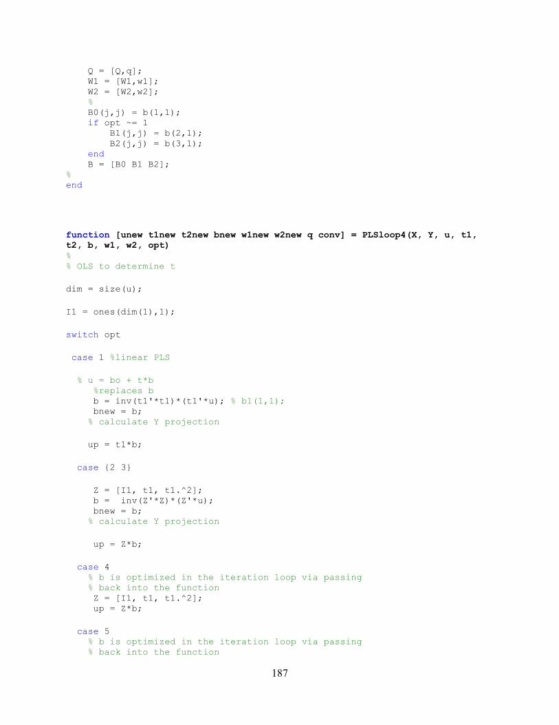
187

Q = [Q,q]; W1 = [W1,w1]; W2 = [W2,w2]; % B0(j,j) = b(1,1); if opt ~= 1 B1(j,j) = b(2,1); B2(j,j) = b(3,1); end B = [B0 B1 B2]; % end

function [unew t1new t2new bnew w1new w2new q conv] = PLSloop4(X, Y, u, t1,

t2, b, w1, w2, opt) % % OLS to determine t

dim = size(u);

I1 = ones(dim(1),1);

switch opt

case 1 %linear PLS

% u = bo + t*b %replaces b b = inv(t1'*t1)*(t1'*u); % b1(1,1); bnew = b; % calculate Y projection

up = t1*b;

case {2 3}

Z = [I1, t1, t1.^2]; b = inv(Z'*Z)*(Z'*u); bnew = b; % calculate Y projection

up = Z*b;

case 4 % b is optimized in the iteration loop via passing % back into the function Z = [I1, t1, t1.^2]; up = Z*b;

case 5 % b is optimized in the iteration loop via passing % back into the function

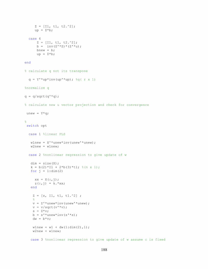
188

Z = [I1, t1, t2.^2]; up = Z*b;

case 6 Z = [I1, t1, t2.^2]; b = inv(Z'*Z)*(Z'*u); bnew = b; up = Z*b;

end

% calculate q not its transpose

q = Y'*up*inv(up'*up); %q( r x 1)

%normalize q

q = q/sqrt(q'*q);

% calculate new u vector projection and check for convergence

unew = Y*q;

% switch opt

case 1 %linear PLS

w1new = X'*unew*inv(unew'*unew); w2new = w1new;

case 2 %nonlinear regression to give update of w

dim = size(X); k = b(2)*I1 + 2*b(3)*t1; %(n x 1); for j = 1:dim(2)

xx = X(:,j); z(:,j) = k.*xx; end

Z = [z, I1, t1, t1.^2] ; % v = Z'*unew*inv(unew'*unew); v = v/sqrt(v'*v); s = Z*v; b = s'*unew*inv(s'*s); dw = b*v;

w1new = w1 + dw(1:dim(2),1); w2new = w1new;

case 3 %nonlinear regression to give update of w assume c is fixed

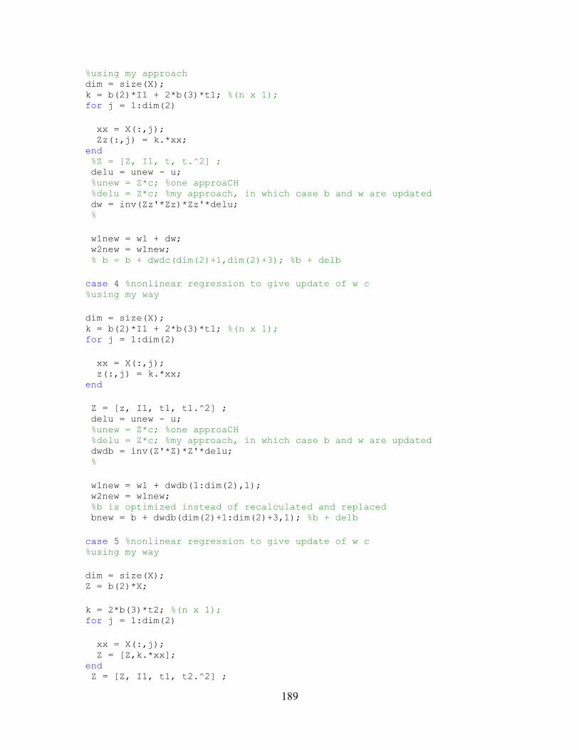
189

%using my approach dim = size(X); k = b(2)*I1 + 2*b(3)*t1; %(n x 1); for j = 1:dim(2)

xx = X(:,j); Zz(:,j) = k.*xx; end %Z = [Z, I1, t, t.^2] ; delu = unew - u; %unew = Z*c; %one approaCH %delu = Z*c; %my approach, in which case b and w are updated dw = inv(Zz'*Zz)*Zz'*delu; %

w1new = w1 + dw; w2new = w1new; % b = b + dwdc(dim(2)+1,dim(2)+3); %b + delb

case 4 %nonlinear regression to give update of w c %using my way

dim = size(X); k = b(2)*I1 + 2*b(3)*t1; %(n x 1); for j = 1:dim(2)

xx = X(:,j); z(:,j) = k.*xx; end

Z = [z, I1, t1, t1.^2] ; delu = unew - u; %unew = Z*c; %one approaCH %delu = Z*c; %my approach, in which case b and w are updated dwdb = inv(Z'*Z)*Z'*delu; %

w1new = w1 + dwdb(1:dim(2),1); w2new = w1new; %b is optimized instead of recalculated and replaced bnew = b + dwdb(dim(2)+1:dim(2)+3,1); %b + delb

case 5 %nonlinear regression to give update of w c %using my way

dim = size(X); Z = b(2)*X;

k = 2*b(3)*t2; %(n x 1); for j = 1:dim(2)

xx = X(:,j); Z = [Z,k.*xx]; end Z = [Z, I1, t1, t2.^2] ;

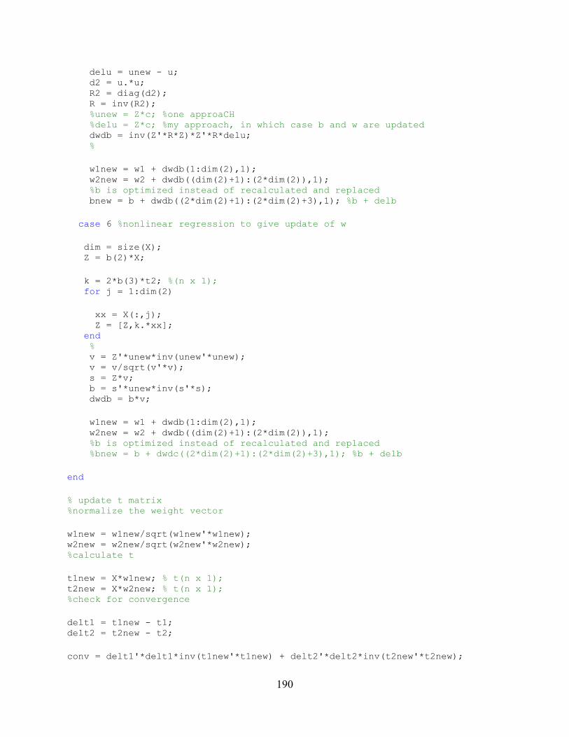
190

delu = unew - u; d2 = u.*u; R2 = diag(d2); R = inv(R2); %unew = Z*c; %one approaCH %delu = Z*c; %my approach, in which case b and w are updated dwdb = inv(Z'*R*Z)*Z'*R*delu; %

w1new = w1 + dwdb(1:dim(2),1); w2new = w2 + dwdb((dim(2)+1):(2*dim(2)),1); %b is optimized instead of recalculated and replaced bnew = b + dwdb((2*dim(2)+1):(2*dim(2)+3),1); %b + delb

case 6 %nonlinear regression to give update of w

dim = size(X); Z = b(2)*X;

k = 2*b(3)*t2; %(n x 1); for j = 1:dim(2)

xx = X(:,j); Z = [Z,k.*xx]; end % v = Z'*unew*inv(unew'*unew); v = v/sqrt(v'*v); s = Z*v; b = s'*unew*inv(s'*s); dwdb = b*v;

w1new = w1 + dwdb(1:dim(2),1); w2new = w2 + dwdb((dim(2)+1):(2*dim(2)),1); %b is optimized instead of recalculated and replaced %bnew = b + dwdc((2*dim(2)+1):(2*dim(2)+3),1); %b + delb

end

% update t matrix %normalize the weight vector

w1new = w1new/sqrt(w1new'*w1new); w2new = w2new/sqrt(w2new'*w2new); %calculate t

t1new = X*w1new; % t(n x 1); t2new = X*w2new; % t(n x 1); %check for convergence

delt1 = t1new - t1; delt2 = t2new - t2;

conv = delt1'*delt1*inv(t1new'*t1new) + delt2'*delt2*inv(t2new'*t2new);

191

Appendix B

Introduction

The appendix provides a more detail explanation and the background theory associated with the

orthogonal and oblique projection mathematics employed in the description of subspace system

identification covered in chapter 3.

B.1 Orthogonal Projection The orthogonal projection of the row space of A into the row space of B is defined as:

!/j = )!j�jj� nj

Where • n denotes the Moore-Penrose pseudo-inverse of the matrix • .

The projection of the row space of A into the orthogonal complement of the row space of B is:

!/jß = )! − !/j

Alternatively Eq. (B.1) maybe represent as:

!/j = )!∏R

where ∏R denotes the operator that projects the row space of a matrix onto the row space of

matrix B:

∏R =)j�jj� nj

192

Likewise∏Rø denotes the geometric operator that projects the row space of a matrix onto the

orthogonal complex of the row space of B:

!/jß = )!∏Rø

where:

∏Rø = zR −∏R

and IB is an identity matrix of the same dimension as B.

The geometric interpretation of these orthogonal projections is depicted in Figure B.1. The

combination of the projections ∏Rø and ∏R decomposes a matrix A into two matrices of which

the row spaces are orthogonal:

! = )!∏Rø + !∏R

The decomposition may also be considered as the representation of the matrix A as linear

combination of the rows of B and of the orthogonal complement of B:

! = )�Røjß + �Rj

Figure B.1 Interpretation of the orthogonal projection in the j-dimensional space (j = 2 in

this case).

B

A

!/j

!/jß

193

B.2 Oblique Projection

The oblique projection of the row space of A along the row space of B into the row space of C is:

!/j� = (!/jß �/jß n�

Figure B.2 illustrates the geometric interpretation of the oblique projection which may be

considered as the linear decomposition of the A unto the row spaces of two non-orthogonal

matrices B and C.

Properties of the orthogonal and oblique projections:

!/!ß = 0 . !/!� = 0 �/!� = ý

Figure B.2 Interpretation of the oblique projection in the j-dimensional space (j = 2 in this

case).

B

C

A

!/j�

194

References

Akaike, H.

1974a NEW LOOK AT STATISTICAL-MODEL IDENTIFICATION. Ieee

Transactions on Automatic Control AC19(6):716-723.

Akaike, H.

1974b STOCHASTIC THEORY OF MINIMAL REALIZATION. Ieee Transactions on

Automatic Control AC19(6):667-674.

Akaike, Hirotugu

1975 Markovian Representation of Stochastic Processes by Canonical Variables.

Society of Industrial and Applied Mathematics - SIAM J Control 13(1):162-173.

Akaike, Hirotugu

1976 Canonical Correlation Analysis of Time Series and the Use of an Information

Criterion. In Mathematics in Science and Engineering. K.M. Raman and G.L. Dimitri,

eds. Pp. 27-96: Elsevier.

Baffi, G., E. B. Martin, and A. J. Morris

1999a Non-linear projection to latent structures revisited (the neural network PLS

algorithm). Computers & Chemical Engineering 23(9):1293-1307.

Baffi, G., E. B. Martin, and A. J. Morris

1999b Non-linear projection to latent structures revisited: the quadratic PLS algorithm.

Computers & Chemical Engineering 23(3):395-411.

Bajpai, R., and M. Reuss

1980 A mechanistic model for penicillin production. Journal of Chemical Technology

and Biotechnology 30:330 - 344.

Birol, G., C. Undey, and A. Cinar

2002 A modular simulation package for fed-batch fermentation: penicillin production.

Computers & Chemical Engineering 26:1553 - 1565.

Borin, A., and R. J. Poppi

2005 Application of mid infrared spectroscopy and iPLS for the quantification of

contaminants in lubricating oil. Vibrational Spectroscopy 37(1):27-32.

Borjas, Santos D. M., and Claudio Garcia

2010 Subspace Identification using the integration of MOESP and N4SID methods

applied to the Shell benchmark of a distillation column. In Proceedings of the 9th

Brazilian Conference on Dynamics, Controls and their Applications Pp. 899 - 904. Serra

Negra, Sao Paulo, Brazil.

Breiman, L., and J. H. Friedman

1997 Predicting multivariate responses in multiple linear regression. Journal of the

Royal Statistical Society Series B-Methodological 59(1):3-37.

Brown, R. G., and P. Y. C. Hwang

1992 Introduction to Random Signals and Applied Kalman Filters: John Wiley and

Sons, Inc.

Buhlmann, P.

1995 THE BLOCKWISE BOOTSTRAP FOR GENERAL EMPIRICAL PROCESSES

OF STATIONARY-SEQUENCES. Stochastic Processes and Their Applications

58(2):247-265.

195

Candy, J. V., Bullock T. E., and Warren M. E.

1979 Invariant Description of the Stochastic Realization. Automatica 15:493-495.

Chen, J. H., and K. C. Liu

2002 On-line batch process monitoring using dynamic PCA and dynamic PLS models.

Chemical Engineering Science 57(1):63-75.

Chen, Q. S., et al.

2008 Determination of total polyphenols content in green tea using FT-NIR

spectroscopy and different PLS algorithms. Journal of Pharmaceutical and Biomedical

Analysis 46(3):568-573.

Chen, Quansheng, Pei Jiang, and Jiewen Zhao

2010 Measurement of total flavone content in snow lotus (Saussurea involucrate) using

near infrared spectroscopy combined with interval PLS and genetic algorithm.

Spectrochim Acta A Mol Biomol Spectrosc 76(1):50-5.

Dejong, S.

1993 SIMPLS - AN ALTERNATIVE APPROACH TO PARTIAL LEAST-SQUARES

REGRESSION. Chemometrics and Intelligent Laboratory Systems 18(3):251-263.

Detroja, K. P., R. D. Gudi, and S. C. Patwardhan

2007 Plant-wide detection and diagnosis using correspondence analysis. Control

Engineering Practice 15(12):1468-1483.

DiCiccio, T. J., and B. Efron

1996 Bootstrap confidence intervals. Statistical Science 11(3):189-212.

Dong, D., and T. J. McAvoy

1996a Batch tracking via nonlinear principal component analysis. Aiche Journal

42(8):2199-2208.

Dong, D., and T. J. McAvoy

1996b Nonlinear principal component analysis - Based on principal curves and neural

networks. Computers & Chemical Engineering 20(1):65-78.

Downs, J. J., and E. F. Vogel

1993 A PLANT-WIDE INDUSTRIAL-PROCESS CONTROL PROBLEM. Computers

& Chemical Engineering 17(3):245-255.

Draper, Norman R., and Harry Smith

1998 Applied Regression Analysis: Wiley-Interscience.

Etezadi-Amoli, J., and R. P. McDonald

1983 A second generation nonlinear factor analysis. Psychometrika 48(3):315-342.

Ferrao, M. F., et al.

2011 Simultaneous determination of quality parameters of biodiesel/diesel blends using

HATR-FTIR spectra and PLS, iPLS or siPLS regressions. Fuel 90(2):701-706.

Frank, I. E., and J. H. Friedman

1993 A STATISTICAL VIEW OF SOME CHEMOMETRICS REGRESSION

TOOLS. Technometrics 35(2):109-135.

Garthwaite, P. H.

1994 AN INTERPRETATION OF PARTIAL LEAST-SQUARES. Journal of the

American Statistical Association 89(425):122-127.

Geladi, Paul, and Bruce R. Kowalski

1986 Partial least-squares regression: a tutorial. Analytica Chimica Acta 185:1-17.

196

Gnanadesikan, R.

1977 Methods for Statistical Data Analysis of Multivariate Observations. New York:

John Wiley and Son Inc.

Haber, R., and H. Unbenhauen

1990 Structure identification of non-linear dynamic systems- A survey on input-output

approaches. Automatica 26(4):651-677.

Hannan, E. J., and B. G. Quinn

1979 DETERMINATION OF THE ORDER OF AN AUTOREGRESSION. Journal of

the Royal Statistical Society Series B-Methodological 41(2):190-195.

Hastie, T., and W. Stuetzle

1989 PRINCIPAL CURVES. Journal of the American Statistical Association

84(406):502-516.

Healy, J.D.

1987 A note on multivariate CUSUM procedures. Technometrics 29:409 - 412.

Helland, I. S.

1988 ON THE STRUCTURE OF PARTIAL LEAST-SQUARES REGRESSION.

Communications in Statistics-Simulation and Computation 17(2):581-607.

Hoskuldsson, A.

1992 QUADRATIC PLS REGRESSION. Journal of Chemometrics 6(6):307-334.

Höskuldsson, Agnar

1988 PLS regression methods. Journal of Chemometrics 2(3):211-228.

Hsieh, William

2001 Nonlinear Canonical Correlation Analysis of Tropical Pacific Climate Variability

Using a Neural Network Approach. Journal of Climate 14(12): 2528-2539.

Hu, K. L., and J. Q. Yuan

2008 Statistical monitoring of fed-batch process using dynamic multiway neighborhood

preserving embedding. Chemometrics and Intelligent Laboratory Systems 90(2):195-203.

Hurvich, C. M., R. Shumway, and C. L. Tsai

1990 IMPROVED ESTIMATORS OF KULLBACK-LEIBLER INFORMATION FOR

AUTOREGRESSIVE MODEL SELECTION IN SMALL SAMPLES. Biometrika

77(4):709-719.

Jolliffe, I.T

2002 Principal component analysis. Aberdeen, UK: Springer-Varlag New York, Inc.

Juricek, B. C., W. E. Larimore, and D. E. Seborg

1999 Reduced-rank ARX and subspace system identification for process control.

Dynamics & Control of Process Systems 1998, Volumes 1 and 2:247-252.

Juricek, B. C., D. E. Seborg, and W. E. Larimore

2005 Process control applications of subspace and regression-based identification and

monitoring methods. ACC: Proceedings of the 2005 American Control Conference, Vols

1-7:2341-2346.

Kegl, B., et al.

1999 A polygonal line algorithm for constructing principal curves. In Advances in

Neural Information Processing Systems 11. M.S. Kearns, S.A. Solla, and D.A. Cohn, eds.

Pp. 501-507. Advances in Neural Information Processing Systems. Cambridge: M I T

Press.

197

Kosanovich, K. A., et al.

1994 MULTIWAY PCA APPLIED TO AN INDUSTRIAL BATCH PROCESS.

Proceedings of the 1994 American Control Conference, Vols 1-3:1294-1298.

Kresta, J. V., J. F. Macgregor, and T. E. Marlin

1991a MULTIVARIATE STATISTICAL MONITORING OF PROCESS OPERATING

PERFORMANCE. Canadian Journal of Chemical Engineering 69(1):35-47.

Kresta, M., J. F. MacGregor, and T.E. Marlin

1991b Multivariate Statistical Monitoring of Process Operating Performance. Canadian

Journal of Chemical Engineers 69:35 - 47.

Ku, Wenfu, Robert H. Storer, and Christos Georgakis

1995 Disturbance detection and isolation by dynamic principal component analysis.

Chemiometrics and intelligent laboratory systems 30:179-196.

Lakshminarayanan, S., P. Mhatre, and R. Gudi

2001 Identification of bilinear models for chemical processes using canonical variate

analysis. Industrial & Engineering Chemistry Research 40(20): 4415-4427

Lakshminarayanan, S., S. L. Shah, and K. Nandakumar

1997 Modeling and control of multivariable processes: Dynamic PLS approach. Aiche

Journal 43(9):2307-2322.

Larimore, W. E.

1996 Statistical optimality and canonical variate analysis system identification. Signal

Processing 52(2):131-144.

Larimore, Wallace E.

1983 System Identification, Reduced Order Filtering and Modelling via Canonical

Variate Analysis. Proceedings from American Control Conference 2:445 - 451.

Larimore, Wallace E.

1990 Canonical Variate Analysis in Identification Filtering and Adaptive Control.

Proceedings of the 28th Conference on Decision and Controls:596-604.

Lee, C., S. W. Choi, and I. B. Lee

2006 Variable reconstruction and sensor fault identification using canonical variate

analysis. Journal of Process Control 16(7):747-761.

Lee, D. S., P. A. Vanrolleghem, and J. M. Park

2005 Parallel hybrid modeling methods for a full-scale cokes wastewater treatment

plant. Journal of Biotechnology 115(3):317-328.

Lee, J. M., C. K. Yoo, and I. B. Lee

2004 Enhanced process monitoring of fed-batch penicillin cultivation using time-

varying and multivariate statistical analysis. Journal of Biotechnology 110(2):119-136.

Li, B. B., E. B. Martin, and A. J. Morris

2001 Box-Tidwell transformation based partial least squares regression. Computers &

Chemical Engineering 25(9-10):1219-1233.

Li, G., S. J. Qin, and D. H. Zhou

2010 Geometric properties of partial least squares for process monitoring. Automatica

46(1):204-210.

Li, T. H., H. Mei, and P. S. Gong

1999 Combining nonlinear PLS with the numeric genetic algorithm for QSAR.

Chemometrics and Intelligent Laboratory Systems 45(1-2):177-184.

198

Li, W., et al.

2000 Recursive PCA for adaptive process monitoring. Journal of Process Control

10(5):471-486.

Liu, R. Y., and J. Tang

1996 Control charts for dependent and independent measurements based on bootstrap

methods. Journal of the American Statistical Association 91(436):1694-1700.

Liu, Yu-ming, Jun Liang, and Ji-xin Qian

2004 The Application of Dynamic Principal Component Analysis to Enhance Chunk

Monitoring of an Industrial Fluidized-Bed Reactor. Proceedings of the 5'h World

Congress on Intelligent Control and Automation, Hangzhou, P.R China, 2004, pp. 1685 -

1688.

Lopes, J. A., et al.

2002 Multiblock PLS analysis of an industrial pharmaceutical process. Biotechnology

and Bioengineering 80(4):419-427.

Lowry, C. A., W. H. Woodhall, and C. W. Champ

1991 A multivariate exponential weighted moving average control chart.

Technometrics 34(1):46 - 53.

Lyman, P. R., and C. Georgakis

1995 Plant-Wide Control of the Tennessee Eastman Problem. Computers & Chemical

Engineering 19(3):321-331.

MacGregor, J. F., et al.

1991 Multivariate statistical methods in process analysis and control. On-line

sensors and data analysis. In Proceedings of the fourth international

conference of chemical processes. Pp. 79 - 94. Padre Island, Texas.

MacGregor, J.F., and T. Kourti

1995 Statistical Process Control of Multivariate Processes. Control Engineering

Practice 3(3):403 - 414

Malthouse, E. C., A. C. Tamhane, and R. S. H. Mah

1997 Nonlinear partial least squares. Computers & Chemical Engineering 21(8):875-

890.

Malthouse, Edward Carl

1995 Nonlinear Partial Least Squares, Statistics Department, Northwestern University.

Martin, E. B., and A. J. Morris

1996 Non-parametric confidence bounds for process performance monitoring charts.

Journal of Process Control 6(6):349-358.

Martin, E. B., A. J. Morris, and J. Zhang

1996 Process performance monitoring using multivariate statistical process control. Iee

Proceedings-Control Theory and Applications 143(2):132-144.

McPherson, L., J. Morris, and E. Martin

2002 Super model-based techniques for batch performance monitoring. In European

Symposium on Computer Aided Process Engineering - 12. J. Grievink and J.

VanSchijndel, eds. Pp. 523-528. Computer-Aided Chemical Engineering. Amsterdam:

Elsevier Science Bv.

McPherson, Lindsay

2007 Model-based Performance Monitroing of Batch Processes, Department of

Chemical Engineering and Advanced Materials, University of Newcastle

199

Morris, A. J., and E. B. Martin

1998 Process performance monitoring and fault detection through multivariate

statistical process control. Oxford: Pergamon Press Ltd.

Negiz, A., and A. Cinar

1997a Statistical Monitoring of Multivariable Dynamic Processes with State Space

Models. AICHE 43(8):2002-2020.

Negiz, A., and A. Cinar

1997b Pls, balanced, and canonical variate realization techniques for identifying

VARMA models in state space

Chemometrics and Intelligent Laboratory Systems 38(2):209-221.

Nomikos, P., and J. F. Macgregor

1994 MONITORING BATCH PROCESSES USING MULTIWAY PRINCIPAL

COMPONENT ANALYSIS. Aiche Journal 40(8):1361-1375.

Nomikos, P., and J. F. MacGregor

1995 Multi-way partial least squares in monitoring batch processes. Chemometrics and

Intelligent Laboratory Systems 30(1):97-108.

Odiowei, P. P., and Y. Cao

2010 State-space independent component analysis for nonlinear dynamic process

monitoring. Chemometrics and Intelligent Laboratory Systems 103(1):59-65.

Oliveira, R.

2004 Combining first principles modelling and artificial neural networks: a general

framework. Computers & Chemical Engineering 28(5):755-766.

Overschee, Peter Van, and Bart De Moor

1995 A Unifying Theorem for Three Subspace System Identification Algorithms.

Automatica, Special issue on Trends in System Identifiction 31(12):1853 - 1864.

Overschee, Peter Van, and Bart De Moor

1996 Subspace identification for linear systems: Theory, implementation. applications.

London: Kluwer Academic Publishers.

Peres, J., R. Oliveira, and S. F. de Azevedo

2001 Knowledge based modular networks for process modelling and control.

Computers & Chemical Engineering 25(4-6):783-791.

Psichogios, D. C., and L. H. Ungar

1992 A HYBRID NEURAL NETWORK-1ST PRINCIPLES APPROACH TO

PROCESS MODELING. Aiche Journal 38(10):1499-1511.

Qin, S. J., and T. J. McAvoy

1992 NONLINEAR PLS MODELING USING NEURAL NETWORKS. Computers &

Chemical Engineering 16(4):379-391.


1993 A DATA-BASED PROCESS MODELING APPROACH AND ITS

APPLICATIONS. Dynamics and Control of Chemical Reactors, Distillation Columns

and Batch Processes ( Dycord Plus 92 ) 1993:93-98.


1996 Nonlinear FIR modeling via a neural net PLS approach. Computers & Chemical

Engineering 20(2):147-159.

200

Ricker, R. L.

1988 The Use of Biased Least-Squares Estimators for Parameters in Discrete-Time

Pulse-Response Models. Industrial & Engineering Chemistry Research 27(2):343-350.

Russell, E. L., L. H. Chiang, and R. D. Braatz

2000 Fault detection in industrial processes using canonical variate analysis and

dynamic principal component analysis. Chemometrics and Intelligent Laboratory

Systems 51(1):81-93.

Schaper, C. D., et al.

1994 IDENTIFICATION OF CHEMICAL PROCESSES USING CANONICAL

VARIATE ANALYSIS. Computers & Chemical Engineering 18(1):55-69.

Schwarz G.

1978 Estimating the dimension of a model. Annals of Statistics 6:461.

Silva, F. E. B., et al.

2009 Simultaneous determination of sulphamethoxazole and trimethoprim in powder

mixtures by attenuated total reflection-Fourier transform infrared and multivariate

calibration. Journal of Pharmaceutical and Biomedical Analysis 49(3):800-805.

Simoglou, A.

1999 Dynamic multivariate statistical process control using partial least squares and

canonical variate analysis. Computers and Chemical Engineering:277 - 280.

Simoglou, A., E. Martin, and J. Morris

1999a A Comparison of Canonical Variate Analysis and Partial Least Squares for the

Identification of Dynamic Processes. Proceedings from American Control Conference

2:832 - 837.

Simoglou, A., E. B. Martin, and A. J. Morris

1999b Dynamic multivariate statistical process control using partial least squares and

canonical variate analysis. Computers & Chemical Engineering 23:S277-S280.

Simoglou, A., E. B. Martin, and A. J. Morris

2002 Statistical performance monitoring of dynamic multivariate processes using state

space modelling. Computers & Chemical Engineering 26(6):909-920.

Van Overschee, P., and B. De Moor

1994 N4SID - SUBSPACE ALGORITHMS FOR THE IDENTIFICATION OF

COMBINED DETERMINISTIC STOCHASTIC-SYSTEMS. Automatica 30(1):75-93.

Verhaegen, M.

1994 Identification of the deterministic part of MIMO state space models given in

inovation from input-output data Automatica 30(1):61 - 74.

Viberg, M., et al.

1993 Performance of subspace based state space system identification methods. In

Proceedings of the 12th IFAC Workd Congress. Pp. 369 - 372, Vol. 7. Sydney, Australia.

von Stosch, M., et al.

2011 A novel identification method for hybrid (N)PLS dynamical systems with

application to bioprocesses. Expert Systems with Applications 38(9):10862-10874.

Wachs, A., and D. R. Lewin

1999 Process monitoring using model-based PCA.

Wangen, L. E., and B. R. Kowalski

1989 A multiblock partial least squares algorithm for investigating complex chemical

systems. Journal of Chemometrics 3(1):3-20.

201

Welch, Greg, and Gary Bishop

2006 An Introduction to Kalman Filters.

http://www.cs.unc.edu/~welch/kalman/kalmanIntro.html.

Willemain, T. R., and G. C. Runger

1996 Designing control charts using an empirical reference distribution. Journal of

Quality Technology 28(1):31-38.

Wise, Barry M., and Neal B. Gallagher

1996 The process chemometrics approach to process monitoring and fault detection.

Journal of Process Control 6(6):329-348.

Wold, S.

1992 NONLINEAR PARTIAL LEAST-SQUARES MODELING .2. SPLINE INNER

RELATION. Chemometrics and Intelligent Laboratory Systems 14(1-3):71-84.

Wold, S., K. Esbensen, and P. Geladi

1987 PRINCIPAL COMPONENT ANALYSIS. Chemometrics and Intelligent

Laboratory Systems 2(1-3):37-52.

Wold , S., et al.

1987 Multiway principal components and PLS-analysis. Journal of Chemometrics 1:41-

56.

Wold, S., N. Kettanehwold, and B. Skagerberg

1989 NONLINEAR PLS MODELING. Chemometrics and Intelligent Laboratory

Systems 7(1-2):53-65.

Yan, Xuefeng

2010 Hybrid artificial neural network based on BP-PLSR and its application in

development of soft sensors. Chemometrics and Intelligent Laboratory Systems

103(2):152-159.

Yao, Y., and F. Gao

2008 Subspace identification for two-dimensional dynamic batch process statistical

monitoring. Chemical Engineering Science 63(13):3411-3418.

Yue, H. H., and S. J. Qin

2001 Reconstruction-based fault identification using a combined index. Industrial &

Engineering Chemistry Research 40(20):4403-4414.

Zhang, J.

2006 Improved on-line process fault diagnosis through information fusion in multiple

neural networks. Computers & Chemical Engineering 30(3):558-571.

Zhang, J., E. B. Martin, and A. J. Morris

1996 Fault detection and diagnosis using multivariate statistical techniques. Chemical

Engineering Research & Design 74(A1):89-96.

Zhao, S. J., J. Zhang, and Y. M. Xu

2006 Performance monitoring of processes with multiple operating modes through

multiple PLS models. Journal of Process Control 16(7):763-772.

Data-Driven, Mechanistic and Hybrid Modelling for ... 12.pdf · Data-Driven, Mechanistic and Hybrid...

Documents

Transcript of Data-Driven, Mechanistic and Hybrid Modelling for ... 12.pdf · Data-Driven, Mechanistic and Hybrid...