Data Collection and AggregationData Collection and Aggregation

1

Challenges: dataChallenges: data

• Data type: numerical sensor readings.

• Rich and massive data, spatially distributed and correlated.

• Data dynamics: data streaming and

2

• Data dynamics: data streaming and aging.

• Uncertainty, noise, erroneous data, outliers.

• Semantics. Raw data � knowledge.

Challenges: query variabilityChallenges: query variability

• Data-centric query: search for “car detection”,

instead of sensor node ID.

• Geographical query: report values near the lake.

• Real-time detection & control: intruder detection.

3

• Real-time detection & control: intruder detection.

• Multi-dimensional query: spatial, temporal and

attribute range.

• Query interface: fixed base station or mobile

hand held devices.

Data processingData processing

• In-network aggregation

• In-network storage

• Distributed data management

• Statistical modeling

4

• Statistical modeling

• Intelligent reasoning

InIn--network data aggregationnetwork data aggregation

• Communication is expensive, bandwidth is precious.

– “In-network processing”: process raw data before transmit.

• Single sensor reading may not hold much

5

• Single sensor reading may not hold much value.

– Inherently unreliable, outlier readings.

– Users are often interested in the hidden patterns or the global picture.

• Data compression and knowledge discovery.– Save storage; generate semantic report.

Distributed InDistributed In--network Storagenetwork Storage• Flash drive, etc. enables distributed in-network

storage

• Challenges

– Distributed indexing for fast query dissemination

6

– Distributed indexing for fast query dissemination

– Explore storage locality to benefit data retrieval.

– Resilience to node or link failures.

– Graceful adaptation to data skews.

– Alleviate the “hot spot” problem created by popular data.

Sound statistical modelsSound statistical models• Raw data may

misrepresent the physical world.– Sensors sample at

discrete times. Sensors may be faulty. Packets may be lost.

7

may be lost.

– Most sensor data may not improve the answer quality to the query. Data can be compressed.

– Correlation between nearby sensors or different attributes of the same sensor.

ModelModel--based querybased query• Build statistical models

on the sensor readings.

– Generates observation plan to improve model accuracy.

– Answers query results.

• Pros:

8

• Pros:

– Improve data robustness.

– Explore correlation

– Decrease communication cost.

– Provide prediction of the future.

– Easier to extract data abstraction.

Reasoning and controlReasoning and control• Reason from raw sensor readings for high-level

semantic events. – Fire detection.

• Events triggered reaction, sensor tasking and control.– Turn on fire alarm. Direct people to closest exits.

9

Data privacy, fault tolerance and securityData privacy, fault tolerance and security

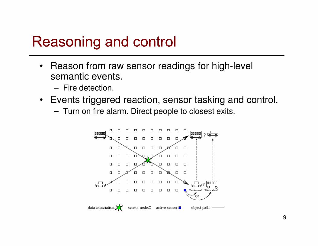
• Under what format should data be stored?

• What if a sensor die? Can we recover its data?

• What information is revealed if a sensor is compromised?

• Adversary injects false reports and false alarms.

10

• Adversary injects false reports and false alarms.

Approximation and randomizationApproximation and randomization• Connection to streaming data model:

– No way to store the raw data.

– Scan the data sequentially.

– Maintain sketches of massive amount of data.

– One more challenge in sensor network: the

11

– One more challenge in sensor network: the streaming data is spatially distributed and communication is expensive.

• Approximations, sampling, randomization.

PapersPapers

• [Madden02] Samuel R. Madden, Michael J. Franklin, Joseph M. Hellerstein, and Wei Hong. TAG: a Tiny AGgregation Service for Ad-Hoc Sensor Networks. OSDI, December 2002. Aggregation with a tree.

• [Shrivastava04] Nisheeth Shrivastava, Chiranjeeb Buragohain, Divy Agrawal, Subhash Suri, Medians and Beyond: New Aggregation Techniques for Sensor Networks, ACM SenSys '04, Nov. 3-5, Baltimore, MD.

12

Networks, ACM SenSys '04, Nov. 3-5, Baltimore, MD. Approximate answer to medians, reduce storage and message size.

• [Nath04] Suman Nath, Phillip B. Gibbons, Zachary Anderson, and Srinivasan Seshan, Synopsis Diffusion for Robust Aggregation in Sensor Networks". In proceedings of ACM

SenSys'04. Use multipath routing to improve routing robustness. Order and duplicate insensitive synopsis needs to be used to prevent one data value to be aggregated multiple times.

TinyDBTinyDB

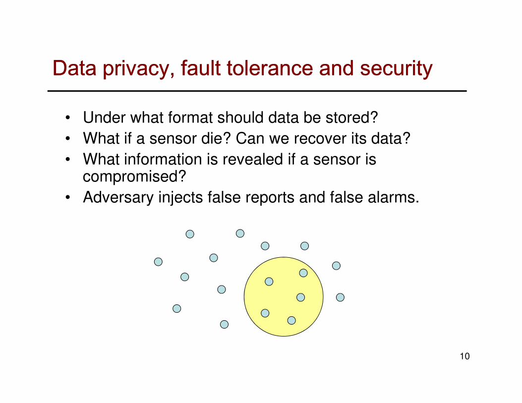
• Philosophy:

– Sensor network = distributed database.

– Data are stored locally.

– Networking structure: tree-based routing.

13

– Networking structure: tree-based routing.

– Top-down SQL query.

– Results aggregated back to the query node.

– Most intelligence outside the network.

TinyDB GUI

TinyDB Client APIDBMS

TinyDB ArchitectureTinyDB Architecture

0

JDBC

Mote side

PC side

14

Sensor network

TinyDB query

processor

0

4

0

1

5

2

6

3

7

Mote side

8

The next few slides from Sam Madden, Wei Hong

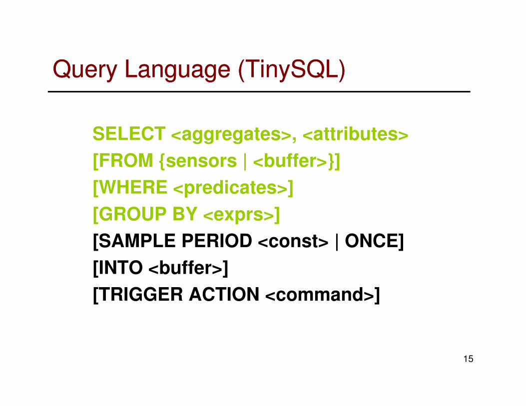
Query Language (TinySQL)Query Language (TinySQL)

SELECT <aggregates>, <attributes>

[FROM {sensors | <buffer>}]

[WHERE <predicates>]

[GROUP BY <exprs>]

15

[GROUP BY <exprs>]

[SAMPLE PERIOD <const> | ONCE]

[INTO <buffer>]

[TRIGGER ACTION <command>]

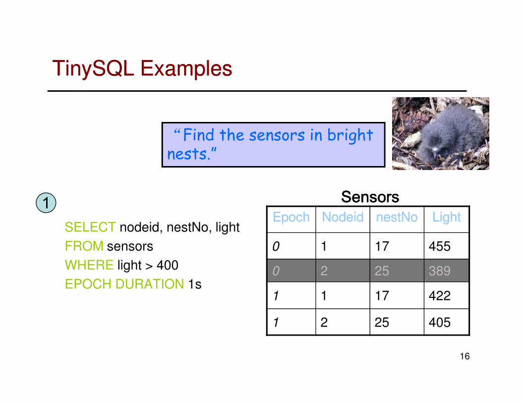
TinySQL ExamplesTinySQL Examples

1 SensorsSensorsSensorsSensors

“Find the sensors in bright nests.”

16

SELECT nodeid, nestNo, light

FROM sensors

WHERE light > 400

EPOCH DURATION 1s

1EpochEpoch NodeidNodeid nestNonestNo LightLight

0 1 17 455

0 2 25 389

1 1 17 422

1 2 25 405

SensorsSensorsSensorsSensors

TinySQL Examples (cont.)TinySQL Examples (cont.)

“Count the number occupied nests in each loud region of the island.”

SELECT AVG(sound)

FROM sensors

EPOCH DURATION 10s

2

17

Epoch region CNT(…) AVG(…)

0 North 3 360

0 South 3 520

1 North 3 370

1 South 3 520

SELECT region, CNT(occupied) AVG(sound)

FROM sensors

GROUP BY region

HAVING AVG(sound) > 200

EPOCH DURATION 10s

3

Regions w/ AVG(sound) > 200

Data ModelData Model

• Entire sensor network as one single, infinitely-long logical table: sensors

• Columns consist of all the attributes defined in the network

• Typical attributes:

18

• Typical attributes:– Sensor readings

– Meta-data: node id, location, etc.

– Internal states: routing tree parent, timestamp, queue length, etc.

• Nodes return NULL for unknown attributes

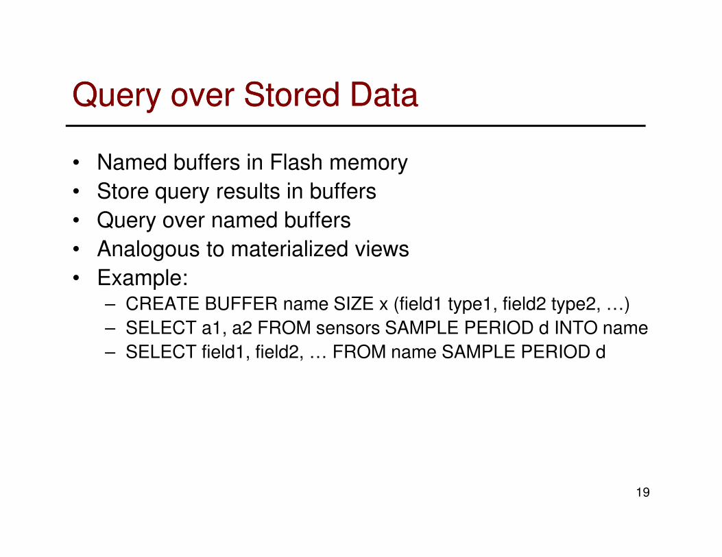
Query over Stored DataQuery over Stored Data

• Named buffers in Flash memory

• Store query results in buffers

• Query over named buffers

• Analogous to materialized views

• Example:

19

• Example:– CREATE BUFFER name SIZE x (field1 type1, field2 type2, …)

– SELECT a1, a2 FROM sensors SAMPLE PERIOD d INTO name

– SELECT field1, field2, … FROM name SAMPLE PERIOD d

EventEvent--based Queriesbased Queries

• ON event SELECT …

• Run query only when interesting events happens

• Event examples– Button pushed

20

– Button pushed

– Message arrival

– Bird enters nest

• Analogous to triggers but events are user-defined

TAG: Tiny AggregationTAG: Tiny Aggregation

• Query Distribution: aggregate queries are pushed

down the network to construct a spanning tree.

– Root broadcasts the query, each node hearing the query broadcasts.

– Each node selects a parent. The routing structure is a

21

spanning tree rooted at the query node.

• Data Collection: aggregate values are routed up

the tree.

– Internal node aggregates the partial data received from its subtree.

TAG exampleTAG example

Query distribution Query collection

1 1

22

2 3

4

56

2 3

4

56

TAG exampleTAG example

MAX AVERAGE

11

23

2 3

4

56

2 3

4

56

m4 = max{m6, m5} Count: c4 = c6+c5Sum: s4 = s6+s5

Considerations about aggregationsConsiderations about aggregations

• Packet loss?

– Acknowledgement and re-transmit?

– Robust routing?

• Packets arriving out of order or in

24

• Packets arriving out of order or in duplicates?

– Double count?

• Size of the aggregates?

– Message size growth?

Classes of aggregationsClasses of aggregations

• Exemplary aggregates return one or more representative values from the set of all values; summary aggregates compute some properties over all values.

25

– MAX, MIN: exemplary; SUM, AVERAGE: summary.

– Exemplary aggregates are prone to packet loss and not amendable to sampling.

– Summary aggregates of random samples can be treated as a robust estimation.

Classes of aggregationsClasses of aggregations

• Duplicate insensitive aggregates are unaffected by duplicate readings.

– Examples: MAX, MIN.

– Independent of routing topology.

26

– Independent of routing topology.

– Combine with robust routing (multi-path).

Classes of aggregationsClasses of aggregations

• Monotonic aggregates: when two partial

records s1 and s2 are combined to s, either

e(s) ≥ max{e(s1), e(s2)} or e(s) ≤ min{e(s1),

e(s2)}.

– Examples: MAX, MIN.

27

– Examples: MAX, MIN.

– Certain predicates (such as HAVING) can be

applied early in the network to reduce the

communication cost.

Classes of aggregationsClasses of aggregations

• Partial state of the aggregates:

– Distributive: the partial state is simply the aggregate for the partial data. The size is the same with the size of the final aggregate. Example: MAX, MIN, SUM

– Algebraic: partial records are of constant size. Example: AVERAGE.

Good

28

AVERAGE.

– Holistic: the partial state records are proportional in size to the partial data. Example: MEDIAN.

– Unique: partial state is proportional to the number of distinct values. Example: COUNT DISTINCT.

– Content-sensitive: partial state is proportional to some (statistical) properties of the data. Example: fixed-size bucket histogram, wavelet, etc.

bad

worst

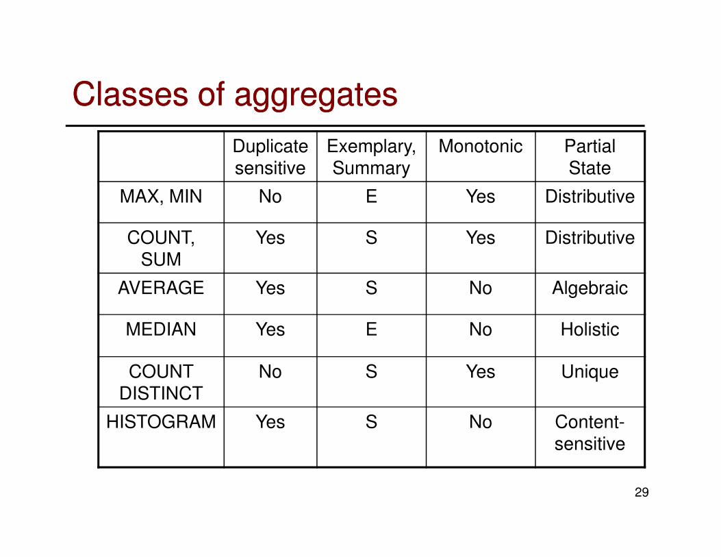
Classes of aggregatesClasses of aggregates

Duplicate sensitive

Exemplary, Summary

Monotonic Partial State

MAX, MIN No E Yes Distributive

COUNT, SUM

Yes S Yes Distributive

AVERAGE Yes S No Algebraic

29

AVERAGE Yes S No Algebraic

MEDIAN Yes E No Holistic

COUNT DISTINCT

No S Yes Unique

HISTOGRAM Yes S No Content-sensitive

Communication costCommunication cost

30

Send all data to the sink

Partial states too large!

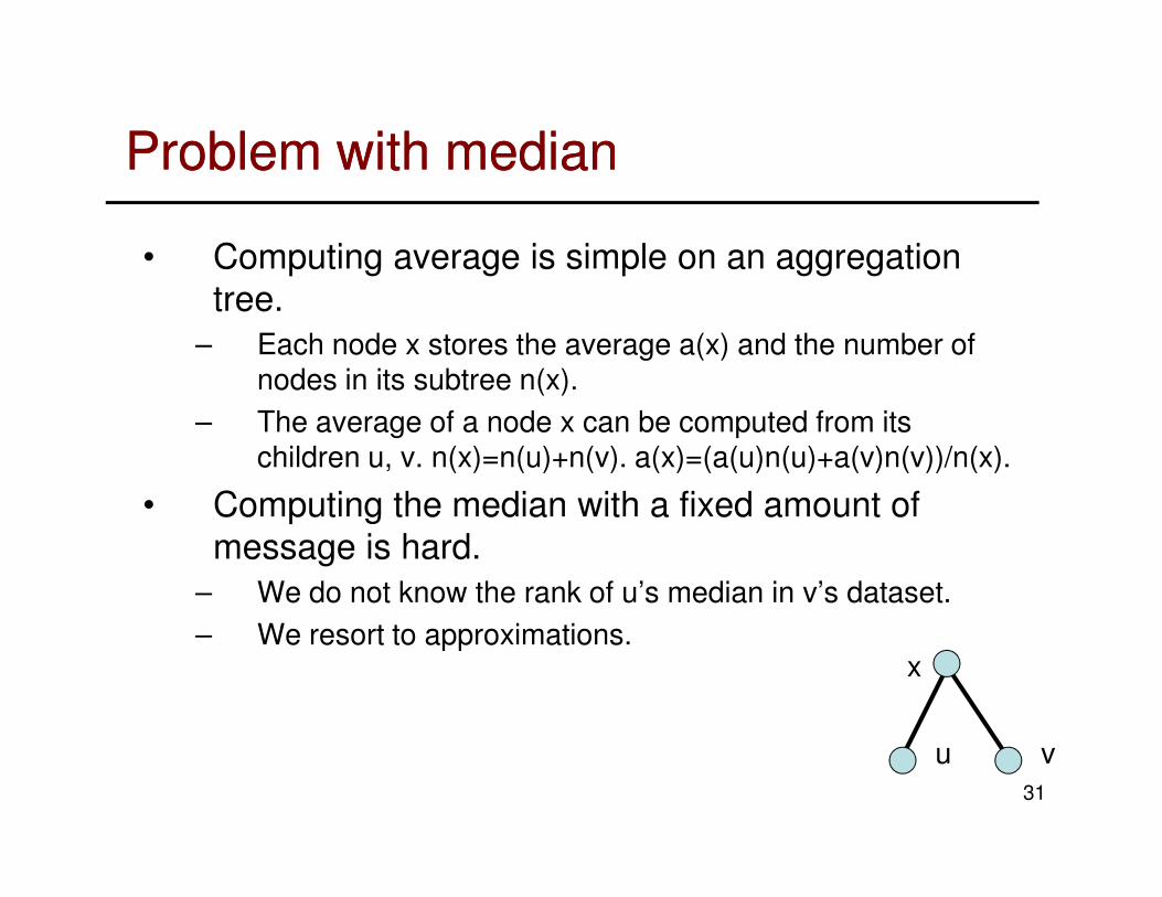
Problem with medianProblem with median

• Computing average is simple on an aggregation

tree.

– Each node x stores the average a(x) and the number of nodes in its subtree n(x).

– The average of a node x can be computed from its children u, v. n(x)=n(u)+n(v). a(x)=(a(u)n(u)+a(v)n(v))/n(x).

31

children u, v. n(x)=n(u)+n(v). a(x)=(a(u)n(u)+a(v)n(v))/n(x).

• Computing the median with a fixed amount of

message is hard.

– We do not know the rank of u’s median in v’s dataset.

– We resort to approximations.x

u v

Deal with computing medianDeal with computing median

• Resort to approximation.

– Random sampling approach.

– A deterministic approach.

32

Approach I: Random samplingApproach I: Random sampling

• Problem: compute the median a of n unsorted elements {ai}.

• Solution: Take a random sample of k elements K. Compute the median x of K.

• Claim: x has rank within (½+ε)n and (½-ε)n

33

• Claim: x has rank within (½+ε)n and (½-ε)n with probability at least 1-2/exp{2kε2}. (Proof left as an exercise.)

• Choose k=ln(2/δ)/(2ε2), then x is an approximate median with probability 1-δ.

Approach II: Quantile digest (qApproach II: Quantile digest (q--digest)digest)

• A data structure that answers

– Approximate quantile query: median, the kth largest reading.

– Range queries: the kth to lth largest readings.

– Most frequent items.

– Histograms.

34

– Histograms.

• Properties:

– Deterministic algorithm.

– Error-memory trade-off.

– Confidence factor.

– Support multiple queries.

QQ--digestdigest

• Input data: frequency of data value {f1, f2,…,fσ}.

• Compress the data:– detailed information concerning frequent data

are preserved;

35

are preserved;

– less frequently occurring values are lumped into larger buckets resulting in information loss.

• Buckets: the nodes in a binary partition of the range [1, σ]. Each bucket v has range [v.min, v.max].

• Only store non-zero buckets.

ExampleExample

Input data bucketed Q-digest

36

Information loss

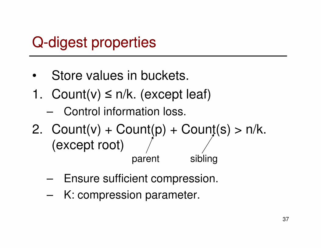
QQ--digest propertiesdigest properties

• Store values in buckets.

1. Count(v) ≤ n/k. (except leaf)

– Control information loss.

2. Count(v) + Count(p) + Count(s) > n/k.

37

2. Count(v) + Count(p) + Count(s) > n/k. (except root)

– Ensure sufficient compression.

– K: compression parameter.

parent sibling

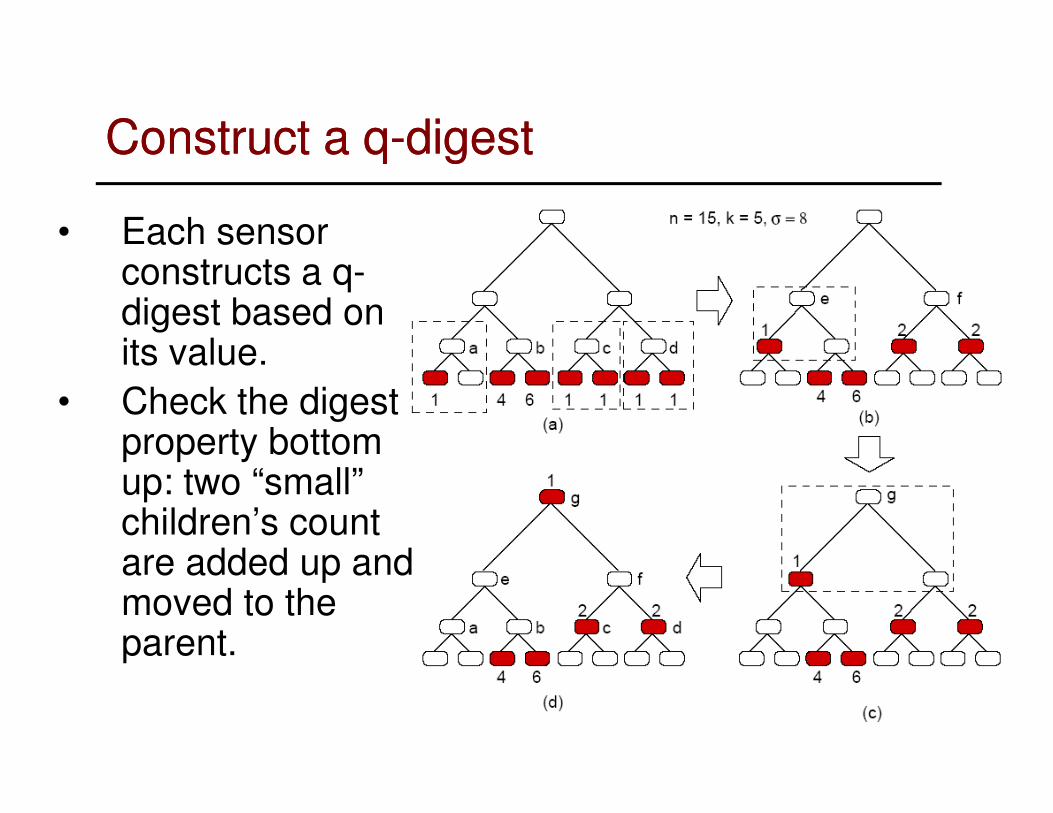
Construct a qConstruct a q--digestdigest

• Each sensor constructs a q-digest based on its value.

• Check the digest

38

• Check the digest property bottom up: two “small” children’s count are added up and moved to the parent.

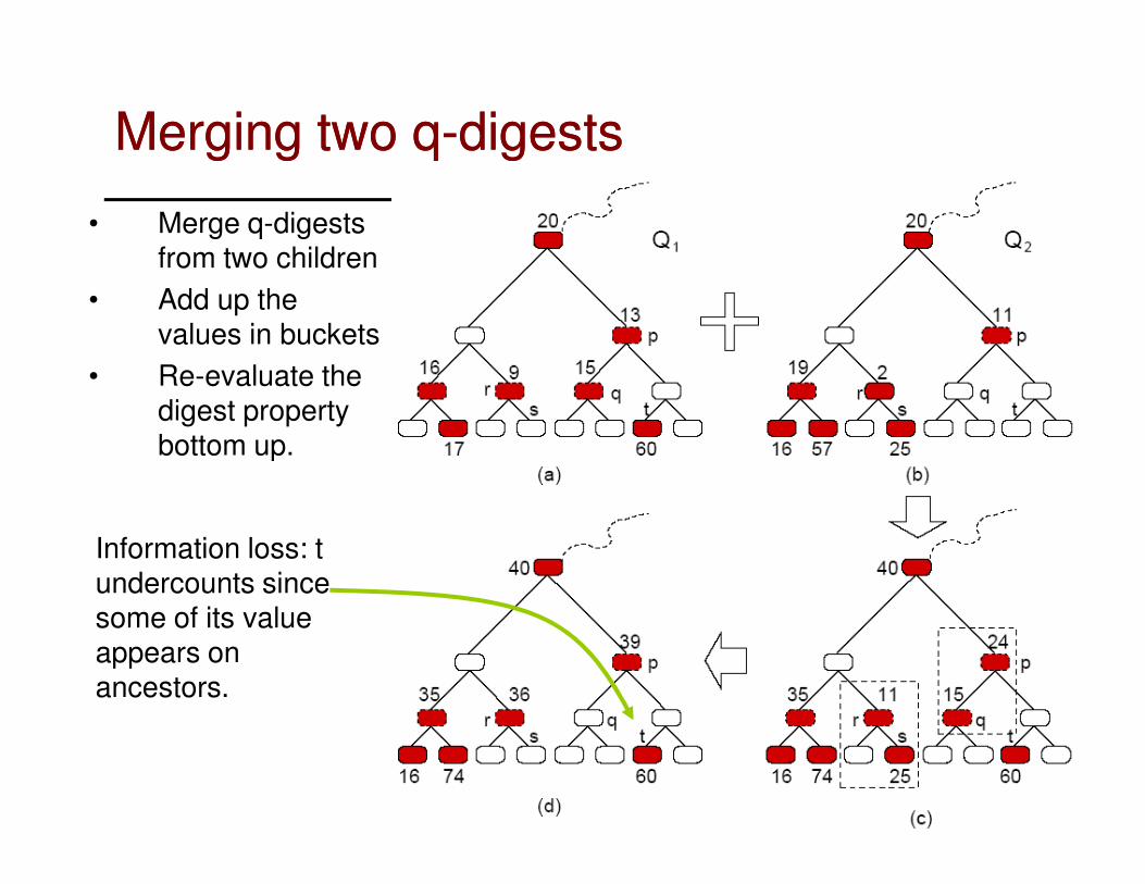
Merging two qMerging two q--digestsdigests

• Merge q-digests from two children

• Add up the values in buckets

• Re-evaluate the digest property bottom up.

39

bottom up.

Information loss: t undercounts since some of its value appears on ancestors.

Space complexitySpace complexity

Claim: A q-digest with compression parameter k has at most 3k buckets.

• By property 2, for all buckets v in Q,

40

– Σv∈Q [Count(v) + Count(p) + Count(s)] > |Q| n/k.

– Σv∈Q [Count(v) + Count(p) + Count(s)] ≤ 3

[Σv∈QCount(v)] = 3n.

– |Q|<3k.

Error boundError bound

Claim: Any value that should be counted in v can be present in one of the ancestors.

1. Count(v) has max error logσ⋅n/k.

41

– Error(v) ≤ Σancestor p Count(p) ≤ Σancestor p n/k ≤

logσ⋅n/k.

2. MERGE maintains the same relative error.– Error(v) ≤ Σi Error(vi) ≤ Σi logσ⋅ni/k ≤ logσ⋅n/k.

Median and quantile queryMedian and quantile query

• Given q∈(0, 1), find the value whose rank is qn.

• Relative error ε=|r-qn|/n, where r is the true rank.

• Post-order traversal on Q, sum the

42

• Post-order traversal on Q, sum the counts of all nodes visited before a node v, which is ≤ # of values less than v.max. Report it when it is first time larger than qn.

• Error bound: ε=logσ /k.

Other queriesOther queries

• Inverse quantile: given a value, determine its rank.– Traverse the tree in post-order, report the sum of counts v

for which x>v.max, which is within [rank(x), rank(x)+εn]

• Range query: find # values in range [l,h].– Perform two inverse quantile queries and take the

43

– Perform two inverse quantile queries and take the difference. Error bound is 2εn.

• Frequent items: given s∈(0, 1), find all values reported by more than sn sensors.

– Count the leaf buckets whose counts are more than (s-ε)n.

– Small false positive: values with count between (s-ε)n and sn may also be reported as frequent.

Simulation setupSimulation setup

• A typical aggregation tree (BFS tree) on 40 nodes

in a 200 by 200 area. In the simulation they use

4000~8000 nodes.

44

Simulation setupSimulation setup

• Random data;

• Correlated data: 3D elevation value from Death

Valley.

45

Histogram v.s. qHistogram v.s. q--digestdigest

• Comparison of histogram and q-digest.

46

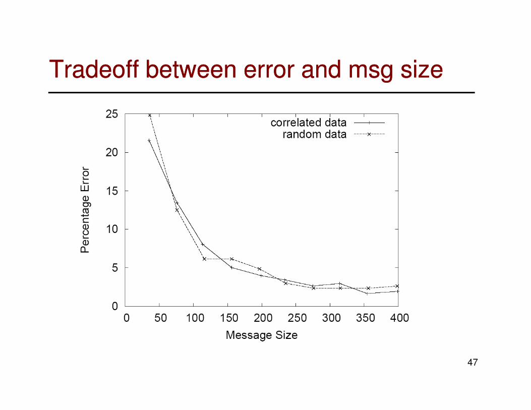
Tradeoff between error and msg sizeTradeoff between error and msg size

47

Saving on message sizeSaving on message size

Naïve solution

48