1

DATA BASE

MANAGEMENT SYSTEM

BCA 202

SELF LEARNING MATERIAL

DIRECTORATE

OF DISTANCE EDUCATION

SWAMI VIVEKANAND SUBHARTI UNIVERSITY

MEERUT – 250 005,

UTTAR PRADESH (INDIA)

2

SLM Module Developed By :

Author:

Reviewed by :

Assessed by:

Study Material Assessment Committee, as per the SVSU ordinance No. VI (2)

Copyright © Gayatri Sales

DISCLAIMER

No part of this publication which is material protected by this copyright notice may be reproduced

or transmitted or utilized or stored in any form or by any means now known or hereinafter invented,

electronic, digital or mechanical, including photocopying, scanning, recording or by any information

storage or retrieval system, without prior permission from the publisher.

Information contained in this book has been published by Directorate of Distance Education and has

been obtained by its authors from sources be lived to be reliable and are correct to the best of their

knowledge. However, the publisher and its author shall in no event be liable for any errors,

omissions or damages arising out of use of this information and specially disclaim and implied

warranties or merchantability or fitness for any particular use.

Published by: Gayatri Sales

Typeset at: Micron Computers Printed at: Gayatri Sales, Meerut.

3

DATA BASE MANAGEMENT SYSTEM

Unit - I

Overview of Database Management System

Elements of Database System, DBMS and its architecture, Advantage of DBMS

(including Data independence), Types of database users, Role of Database

administrator.

Unit - II

Data Models

Brief overview of Hierarchical and Network Model, Detailed study of Relational Model

(Relations, Properties, Key & Integrity rules), Comparison of Hierarchical, Network and

Relational Model ,CODD‘s rules for Relational Model,E-R diagram.

Unit - III

Normalization

Normalization concepts and update anomalies ,Functional dependencies,Multivalued

and join dependencies.

Normal Forms: (1 NF, 2 NF, 3NF, BCNF, 4NF, and 5NF)

Unit - IV

SQL

SQL Constructs, SQL Join: Multiple Table Queries, Build-in functions, Views and their

use, Overviews of ORACLE: (Data definition and manipulation)

Unit - V

Database Security, Integrity and Control

Security and Integrity threats, Defense mechanism, Integrity, Auditing and Control,

Recent trends in DBMS- Distributed and Deductive Database.

4

UNIT - I

Overview of Database Management System

Elements of Database System

Organizations produce and gather data as they operate. Contained in a database, data is typically organized to model relevant aspects of reality in a way that supports processes requiring this information. Knowing how this can be managed effectively is vital to any organization.

What is a Database Management System (or DBMS)?

Organizations employ Database Management Systems (or DBMS) to help them effectively manage their data and derive relevant information out of it. A DBMS is a technology tool that directly supports data management. It is a package designed to define, manipulate, and manage data in a database. Some general functions of a DBMS:

Designed to allow the definition, creation, querying, update, and administration of databases

Define rules to validate the data and relieve users of framing programs for data maintenance

Convert an existing database, or archive a large and growing one

Run business applications, which perform the tasks of managing business processes, interacting with end-users and other applications, to capture and analyze data

Some well-known DBMSs are Microsoft SQL Server, Microsoft Access, Oracle, SAP, and others.

Components of DBMS

DBMS have several components, each performing very significant tasks in the database management system environment. Below is a list of components within the database and its environment.

Software This is the set of programs used to control and manage the overall database. This includes the DBMS software itself, the Operating System, the network software being used to share the data among users, and the application programs used to access data in the DBMS.

5

Hardware Consists of a set of physical electronic devices such as computers, I/O devices, storage devices, etc., this provides the interface between computers and the real world systems. Data DBMS exists to collect, store, process and access data, the most important component. The database contains both the actual or operational data and the metadata. Procedures These are the instructions and rules that assist on how to use the DBMS, and in designing and running the database, using documented procedures, to guide the users that operate and manage it. Database Access Language This is used to access the data to and from the database, to enter new data, update existing data, or retrieve required data from databases. The user writes a set of appropriate commands in a database access language, submits these to the DBMS, which then processes the data and generates and displays a set of results into a user readable form. Query Processor This transforms the user queries into a series of low level instructions. This reads the online user‘s query and translates it into an efficient series of operations in a form capable of being sent to the run time data manager for execution. Run Time Database Manager Sometimes referred to as the database control system, this is the central software component of the DBMS that interfaces with user-submitted application programs and queries, and handles database access at run time. Its function is to convert operations in user‘s queries. It provides control to maintain the consistency, integrity and security of the data. Data Manager Also called the cache manger, this is responsible for handling of data in the database, providing a recovery to the system that allows it to recover the data after a failure. Database Engine The core service for storing, processing, and securing data, this provides controlled access and rapid transaction processing to address the requirements of the most demanding data consuming applications. It is often used to create relational databases for online transaction processing or online analytical processing data. Data Dictionary This is a reserved space within a database used to store information about the database itself. A data dictionary is a set of read-only table and views, containing the

6

different information about the data used in the enterprise to ensure that database representation of the data follow one standard as defined in the dictionary. Report Writer Also referred to as the report generator, it is a program that extracts information from one or more files and presents the information in a specified format. Most report writers allow the user to select records that meet certain conditions and to display selected fields in rows and columns, or also format the data into different charts.

Great Performance through Effective DBMS

A company‘s performance is greatly affected by how it manages its data. And one of the most basic tasks of data management is the effective management of its database. Understanding the different components of the DBMS and how it works and relates to each other is the first step to employing an effective DBMS.

DBMS and its architecture

The design of a DBMS depends on its architecture. It can be centralized or decentralized or hierarchical. The architecture of a DBMS can be seen as either single tier or multi-tier. An n-tier architecture divides the whole system into related but independent n modules, which can be independently modified, altered, changed, or replaced.

In 1-tier architecture, the DBMS is the only entity where the user directly sits on the DBMS and uses it. Any changes done here will directly be done on the DBMS itself. It does not provide handy tools for end-users. Database designers and programmers normally prefer to use single-tier architecture.

If the architecture of DBMS is 2-tier, then it must have an application through which the DBMS can be accessed. Programmers use 2-tier architecture where they access the DBMS by means of an application. Here the application tier is entirely independent of the database in terms of operation, design, and programming.

Architecture

Database architecture uses programming languages to design a particular type of

software for businesses or organizations.Database architecture focuses on the design,

development, implementation and maintenance of computer programs that store and

organize information for businesses, agencies and institutions. A database architect

develops and implements software to meet the needs of users.

The design of a DBMS depends on its architecture. It can be centralized or decentralized

or hierarchical. The architecture of a DBMS can be seen as either single tier or multi-tier.

The tiers are classified as follows :

7

1. 1-tier architecture

2. 2-tier architecture

3. 3-tier architecture

4. n-tier architecture

1-tier architecture:

One-tier architecture involves putting all of the required components for a software

application or technology on a single server or platform.

1-tier architecture

Basically, a one-tier architecture keeps all of the elements of an application, including the

interface, Middleware and back-end data, in one place. Developers see these types of

systems as the simplest and most direct way.

8

2-tier architecture:

The two-tier is based on Client Server architecture. The two-tier architecture is like client

server application. The direct communication takes place between client and server.

There is no intermediate between client and server.

2-tier architecture

3-tier architecture:

A 3-tier architecture separates its tiers from each other based on the complexity of the

users and how they use the data present in the database. It is the most widely used

architecture to design a DBMS.

9

This architecture has different usages with different applications. It can be used in web

applications and distributed applications. The strength in particular is when using this

architecture over distributed systems.

Database (Data) Tier −

At this tier, the database resides along with its query processing languages. We also

have the relations that define the data and their constraints at this level.

Application (Middle) Tier −

At this tier reside the application server and the programs that access the database.

For a user, this application tier presents an abstracted view of the database. End-

users are unaware of any existence of the database beyond the application. At the

other end, the database tier is not aware of any other user beyond the application

10

tier. Hence, the application layer sits in the middle and acts as a mediator between

the end-user and the database.

User (Presentation) Tier −

End-users operate on this tier and they know nothing about any existence of the

database beyond this layer. At this layer, multiple views of the database can be

provided by the application. All views are generated by applications that reside in the

application tier.

n-tier architecture:

N-tier architecture would involve dividing an application into three different tiers. These

would be the

1. logic tier,

2. the presentation tier, and

3. the data tier.

It is the physical separation of the different parts of the application as opposed to the

usually conceptual or logical separation of the elements in the model-view-controller

(MVC) framework. Another difference from the MVC framework is that n-tier layers are

connected linearly, meaning all communication must go through the middle layer, which

is the logic tier. In MVC, there is no actual middle layer because the interaction is

triangular; the control layer has access to both the view and model layers and the model

also accesses the view; the controller also creates a model based on the requirements

and pushes this to the view. However, they are not mutually exclusive, as the MVC

framework can be used in conjunction with the n-tier architecture, with the n-tier being

the overall architecture used and MVC used as the framework for the presentation tier.

Normalization of Database:

Database Normalisation is a technique of organizing the data in the database.

Normalization is a systematic approach of decomposing tables to eliminate data

redundancy and undesirable characteristics like Insertion, Update and Deletion

Anamolies. It is a multi-step process that puts data into tabular form by removing

duplicated data from the relation tables.

11

Normalization is used for mainly two purpose,

Eliminating reduntant(useless) data.

Ensuring data dependencies make sense i.e data is logically stored.

Problem Without Normalization:

Without Normalization, it becomes difficult to handle and update the database, without

facing data loss. Insertion, Updation and Deletion Anamolies are very frequent if

Database is not Normalized.

Normalization Rule:

Normalization rule are divided into following normal form.

1. First Normal Form

2. Second Normal Form

3. Third Normal Form

4. BCNF

First Normal Form:

A database is in first normal form if it satisfies the following conditions:

Contains only atomic values

There are no repeating groups

An atomic value is a value that cannot be divided. For example, in the table shown

below, the values in the [Color] column in the first row can be divided into ―red‖ and

―green‖, hence [TABLE_PRODUCT] is not in 1NF.

12

A repeating group means that a table contains two or more columns that are closely

related. For example, a table that records data on a book and its author(s) with the

following columns: [Book ID], [Author 1], [Author 2], [Author 3] is not in 1NF because

[Author 1], [Author 2], and [Author 3] are all repeating the same attribute.

1st Normal Form Example

How do we bring an unnormalized table into first normal form? Consider the following

example:

This table is not in first normal form because the [Color] column can contain multiple

values. For example, the first row includes values ―red‖ and ―green.‖

To bring this table to first normal form, we split the table into two tables and now we have

the resulting tables:

13

Now first normal form is satisfied, as the columns on each table all hold just one value.

Second Normal Form:

A database is in second normal form if it satisfies the following conditions:

It is in first normal form

All non-key attributes are fully functional dependent on the primary key

In a table, if attribute B is functionally dependent on A, but is not functionally dependent

on a proper subset of A, then B is considered fully functional dependent on A. Hence, in

a 2NF table, all non-key attributes cannot be dependent on a subset of the primary key.

Note that if the primary key is not a composite key, all non-key attributes are always fully

functional dependent on the primary key. A table that is in 1st normal form and contains

only a single key as the primary key is automatically in 2nd normal form.

2nd Normal Form Example

Consider the following example:

This table has a composite primary key [Customer ID, Store ID]. The non-key attribute is

[Purchase Location]. In this case, [Purchase Location] only depends on [Store ID], which

is only part of the primary key. Therefore, this table does not satisfy second normal form.

14

To bring this table to second normal form, we break the table into two tables, and now

we have the following:

What we have done is to remove the partial functional dependency that we initially had.

Now, in the table [TABLE_STORE], the column [Purchase Location] is fully dependent

on the primary key of that table, which is [Store ID].

Third Normal Form:

A relation is in third normal form if it is in 2NF and no non key attribute is transitively

dependent on the primary key.

A bank uses the following relation:

Vendor(ID, Name, Account_No, Bank_Code_No, Bank)

The attribute ID is the identification key. All attributes are single valued (1NF). The table

is also in 2NF.

The following dependencies exist:

15

1. Name, Account_No, Bank_Code_No are functionally dependent on ID (ID → Name,

Account_No, Bank_Code_No)

2. Bank is functionally dependent on Bank_Code_No (Bank_Code_No → Bank)

The table in this example is in 1NF and in 2NF. But there is a transitive dependency

between Bank_Code_No and Bank, because Bank_Code_No is not the primary key of

this relation. To get to the third normal form (3NF), we have to put the bank name in a

separate table together with the clearing number to identify it.

BCNF:

BCNF was developed by Raymond Boyce and E.F. Codd; the latter is widely considered

the father of relational database design.

BCNF is really an extension of 3rd Normal Form (3NF). For this reason it is frequently

termed 3.5NF. 3NF states that all data in a table must depend only on that table‘s

primary key, and not on any other field in the table. At first glance it would seem that

BCNF and 3NF are the same thing. However, in some rare cases it does happen that a

3NF table is not BCNF-compliant. This may happen in tables with two or more

overlapping composite candidate keys.

Advantage of DBMS (including Data independence)

The database management system has a number of advantages as compared to traditional computer file-based processing approach. The DBA must keep in mind these benefits or capabilities during databases and monitoring the DBMS. The Main advantages of DBMS are described below.

Centralized Data Management: Large commercial databases may exist in two different Topologies.

1. Centralized A centralized database (sometimes abbreviated CDB) is a database that is located, stored, and maintained in a single location. This location is most often a central computer or database system, for example a desktop or server, or a mainframe computer. Users typically use an Internet connection and network of computers to access a CDB. In most cases, a centralized database would be used by an organization (e.g. a business company) or an institution (e.g. a university). Banks, airlines, railways etc., tend to use centralized databases.

2. Distributed Where the database is in many locations often where you have a national or international company and customers tend to regularly interact with a

16

local branch. For example: Google uses a distributed DBMS to cater to users in different geographic regions to dispense country/region specific information.

In both cases the database looks like one database the end-user cannot feel the difference. Information stored in Centralized databases is accessible from a large number of different points, which in turn creates a significant amount of advantages as against other types of databases. Some of the important advantages are listed below:

1. Data integrity is maximized and data redundancy is minimized, as the single storing place of all the data also implies that a given set of data only has one primary record. This helps in maintaining data accurately and consistently, hence enhancing data reliability.

2. Generally bigger data security, as the single data storage location implies that there is only one possible place where the database can be attacked and sets of data can be stolen or tampered with.

3. Better data preservation than the distributed type since data backup and maintenance becomes easier and less time consuming.

4. Ease of use by the end-user due to the simplicity of a single database design.

5. Generally easier data portability and database administration.

6. More cost effective than other types of database systems as labor, power supply and maintenance costs are all minimized.

7. Data kept in the same location is easier to be edited, updated, re-organized, mirrored, or analyzed.

8. All the information can be accessed at the same time from the same location.

9. Updates to any given set of data are immediately received by every end-user.

Data Independence: In a database, the management system provides the interface between the application programs and the data. Data independence refers to the immunity of user applications to changes made in the data structure and organization or storage. Physical data independence means the applications need not worry about how the data are physically structured and stored. Applications should work with a logical data model and declarative query language.

If major changes were to be made to the data, the application programs may need to be rewritten. When changes are made to the data representation, the data maintained by the DBMS is changed but the DBMS continues to provide data to application programs in the previously used ways.

Data independence is the immunity of application programs to changes in storage structures and access techniques. For example if we add a new attribute, change index structure then in traditional file processing system, the applications are affected. But in a DBMS environment these changes are reflected in the catalog. As a result the applications are not affected. Data independence can be physical data independence or logical data independence.

17

� Physical data independence is the ability to modify physical schema without causing the conceptual schema or application programs to be rewritten. In effect, it means that different kinds of user applications are able to interact with the data irrespective of the structure of the data in the database.

� Logical data independence is the ability to modify the conceptual schema without having to change the external schemas or application programs. Logical Data independence means if we add some new columns or remove some columns from table then the user view and programs will not change.

Data independence and operation independence together define Data Abstraction.

Data Inconsistency: Data inconsistency means different copies of the same data will have different values. For example, consider a person working in a branch of an organization.

The details of the person will be stored both in the branch office as well as in the main office. If that particular person changes his address, then the change of address has to be maintained in the main as well as the branch office. For example the change of address is maintained in the branch office but not in the main office, then the data about that person is inconsistent.

DBMS is designed to have data consistency. Some of the qualities achieved in DBMS are:

1. Data redundancy → Reduced in DBMS.

2. Data independence → Activated in DBMS.

3. Data inconsistency → Avoided in DBMS.

4. Centralizing the data → Achieved in DBMS.

5. Data integrity → Necessary for efficient Transaction.

6. Support for multiple views → Necessary for security reasons.

Explanation of Terms:

� Data redundancy means duplication of data. Data redundancy will occupy more space hence it is not desirable.

� Data independence means independence between application program and the data. The advantage is that when the data representation changes, it is not necessary to change the application program.

� Data inconsistency means different copies of the same data will have different values.

� Centralizing the data means data can be easily shared between the users but the main concern is data security.

� The main threat to data integrity comes from several different users attempting to update the same data at the same time. For example, The number of bookings made is larger than the capacity of the aircraft/train.

18

� Support for multiple views means DBMS allows different users to see different views of the database, according to the perspective each one requires. This concept is used to enhance the security of the database.

Other Advantages of DBMS

Controlling Data Redundancy In non-database systems each application program has its own private files. In this case, the duplicated copies of the same data is created in many places. In DBMS, all data of an organization is integrated into a single database file. The data is recorded in only one place in the database and it is not duplicated.

Data Sharing In DBMS, data can be shared by authorized users of the organization. The database administrator manages the data and gives rights to users to access the data. Many users can be authorized to access the same piece of information simultaneously. The remote users can also share same data. Similarly, the data of same database can be shared between different application programs.

Data Consistency By controlling the data redundancy, the data consistency is obtained. If a data item appears only once, any update to its value has to be performed only once and the updated value is immediately available to all users. If the DBMS has controlled redundancy, the database system enforces consistency.

Data Integration In Database management system, data in database is stored in tables. A single database contains multiple tables and relationships can be created between tables (or associated data entities). This makes easy to retrieve and update data.

Integration Constraints

Integrity constraints or consistency rules can be applied to database so that the correct data can be entered into database. The constraints may be applied to data item within a single record or they may be applied to relationships between records.

Data Security Form is very important object of DBMS. You can create forms very easily and quickly in DBMS. Once a form is created, it can be used many times and it can be modified very easily. The created forms are also saved along with database and behave like a software component. A form provides very easy way (user-friendly) to enter data into database, edit data and display data from database. The non-technical users can also perform various operations on database through forms without going into technical details of a fatabase.

Report Writing

19

Most of the DBMSs provide the report writer tools used to create reports. The users can create very easily and quickly. Once a report is created, it can be used may times and it can be modified very easily. The created reports are also saved along with database and behave like a software component.

Control over Concurrency In a computer file-based system, if two users are allowed to access data simultaneously, it is possible that they will interfere with each other. For example, if both users attempt to perform update operation on the same record, then one may overwrite the values recorded by the other. Most database management systems have sub-systems to control the concurrency so that transactions are always recorded with accuracy.

Backup and Recovery Procedures In a computer file-based system, the user creates the backup of data regularly to protect the valuable data from damage due to failures to the computer system or application program. It is very time consuming method, if amount of data is large. Most of the DBMSs provide the 'backup and recovery' sub-systems that automatically create the backup of data and restore data if required.

Data Independence is defined as a property of DBMS that helps you to change the Database schema at one level of a database system without requiring to change the schema at the next higher level. Data independence helps you to keep data separated from all programs that make use of it.

You can use this stored data for computing and presentation. In many systems, data independence is an essential function for components of the system.

In this tutorial, you will learn:

What is Data Independence of DBMS?

Types of Data Independence

Levels of Database

Physical Data Independence

Logical Data Independence

Difference between Physical and Logical Data Independence

Importance of Data Independence

20

Types of Data Independence

In DBMS there are two types of data independence

1. Physical data independence

2. Logical data independence.

Levels of Database

Before we learn Data Independence, a refresher on Database Levels is important. The database has 3 levels as shown in the diagram below

1. Physical/Internal

2. Conceptual

3. External

Consider an Example of a University Database. At the different levels this is how the implementation will look like:

Type of Schema Implementation

External Schema View 1: Course info(cid:int,cname:string)

View 2: studeninfo(id:int. name:string)

Conceptual Shema Students(id: int, name: string, login: string,

age: integer)

Courses(id: int, cname.string, credits:integ

er)

Enrolled(id: int, grade:string)

Physical Schema Relations stored as unordered files.

Index on the first column of

Students.

Physical Data Independence

21

Physical data independence helps you to separate conceptual levels from the internal/physical levels. It allows you to provide a logical description of the database without the need to specify physical structures. Compared to Logical Independence, it is easy to achieve physical data independence.

With Physical independence, you can easily change the physical storage structures or devices with an effect on the conceptual schema. Any change done would be absorbed by the mapping between the conceptual and internal levels. Physical data independence is achieved by the presence of the internal level of the database and then the transformation from the conceptual level of the database to the internal level.

Examples of changes under Physical Data Independence

Due to Physical independence, any of the below change will not affect the conceptual layer.

Using a new storage device like Hard Drive or Magnetic Tapes

Modifying the file organization technique in the Database

Switching to different data structures.

Changing the access method.

Modifying indexes.

Changes to compression techniques or hashing algorithms.

Change of Location of Database from say C drive to D Drive

Logical Data Independence

Logical Data Independence is the ability to change the conceptual scheme without changing

1. External views

2. External API or programs

Any change made will be absorbed by the mapping between external and conceptual levels.

When compared to Physical Data independence, it is challenging to achieve logical data independence.

22

Examples of changes under Logical Data Independence

Due to Logical independence, any of the below change will not affect the external layer.

1. Add/Modify/Delete a new attribute, entity or relationship is possible without a rewrite of existing application programs

2. Merging two records into one

3. Breaking an existing record into two or more records

Difference between Physical and Logical Data Independence

Logica Data Independence Physical Data Independence

Logical Data Independence is mainly

concerned with the structure or changing

the data definition.

Mainly concerned with the storage of the

data.

It is difficult as the retrieving of data is

mainly dependent on the logical structure

of data.

It is easy to retrieve.

Compared to Logic Physical

independence it is difficult to achieve

logical data independence.

Compared to Logical Independence it is

easy to achieve physical data

independence.

You need to make changes in the

Application program if new fields are

added or deleted from the database.

A change in the physical level usually

does not need change at the Application

program level.

Modification at the logical levels is

significant whenever the logical structures

of the database are changed.

Modifications made at the internal levels

may or may not be needed to improve the

performance of the structure.

Concerned with conceptual schema Concerned with internal schema

23

Example: Add/Modify/Delete a new

attribute

Example: change in compression

techniques, hashing algorithms, storage

devices, etc

Importance of Data Independence

Helps you to improve the quality of the data

Database system maintenance becomes affordable

Enforcement of standards and improvement in database security

You don't need to alter data structure in application programs

Permit developers to focus on the general structure of the Database rather than worrying about the internal implementation

It allows you to improve state which is undamaged or undivided

Database incongruity is vastly reduced.

Easily make modifications in the physical level is needed to improve the performance of the system.

Summary

Data Independence is the property of DBMS that helps you to change the Database schema at one level of a database system without requiring to change the schema at the next higher level.

Two levels of data independence are 1) Physical and 2) Logical

Physical data independence helps you to separate conceptual levels from the internal/physical levels

Logical Data Independence is the ability to change the conceptual scheme without changing

When compared to Physical Data independence, it is challenging to achieve logical data independence

Data Independence Helps you to improve the quality of the data

24

Types of database users

This differentiation is made according to the interaction of users to the database.

Database system is made to store information and provide an environment for retrieving

information. There are four types of database users in DBMS we are going to discuss in

this article.

Different Types of Database Users in DBMS Application Programmers

As its name shows, application programmers are the one who writes application programs that uses the database. These application programs are written in programming languages like COBOL or PL (Programming Language 1), Java and fourth generation language. These programs meet the user requirement and made according to user requirements. Retrieving information, creating new information and changing existing information is done by these application programs. They interact with DBMS through DML (Data manipulation language) calls. And all these functions are performed by generating a request to the DBMS. If application programmers are not there then there will be no creativity in the whole team of Database. End Users

End users are those who access the database from the terminal end. They use the developed applications and they don‘t have any knowledge about the design and working of database. These are the second class of users and their main motto is just to get their task done. There are basically two types of end users that are discussed below. Casual User These users have great knowledge of query language. Casual users access data by entering different queries from the terminal end. They do not write programs but they can interact with the system by writing queries. Naïve Any user who does not have any knowledge about database can be in this category. There task is to just use the developed application and get the desired results. For example: Clerical staff in any bank is a naïve user. They don‘t have any dbms knowledge but they still use the database and perform their given task.

25

DBA (Database Administrator)

DBA can be a single person or it can be a group of person. Database Administrator is responsible for everything that is related to database. He makes the policies, strategies and provides technical supports. System Analyst

System analyst is responsible for the design, structure and properties of database. All the requirements of the end users are handled by system analyst. Feasibility, economic and technical aspects of DBMS is the main concern of system analyst. Role of Database administrator Role, Duties and Responsibilities of database Administrator( DBA): There are lots of role and duties of a database administrator (DBA). He is responsible for managing, securing and taking care of the database system. So before we start discussing the role and duties of DBA, we should understand who DBA is in actual and what is he meant for? Who Is A DBA (Database Administrator)

A Database Administrator is a person or a group of person who are responsible for managing all the activities related to database system. This job requires a high level of expertise by a person or group of person. There are very rare chances that only a single person can manage all the database system activities so companies always have a group of people who take care of database system. In a nut shell, A DBA is the controller of everything related to database system. Now let us discuss what are the main role and duties of Database Administrator (DBA). Role, Duties and Responsibilities of database Administrator( DBA) Installing and Configuration of database: DBA is responsible for installing the database software. He configure the software of database and then upgrades it if needed. There are many database software like oracle, Microsoft SQL and MySQL in the industry so DBA decides how the installing and configuring of these database software will take place. 1. Deciding the hardware device

Depending upon the cost, performance and efficiency of the hardware, it is DBA who have the duty of deciding which hardware devise will suit the company requirement. It is hardware that is an interface between end users and database so it needed to be of best quality.

26

2. Managing Data Integrity

Data integrity should be managed accurately because it protects the data from unauthorized use. DBA manages relationship between the data to maintain data consistency. 3. Decides Data Recovery and Back up method

If any company is having a big database, then it is likely to happen that database may fail at any instance. It is require that a DBA takes backup of entire database in regular time span. DBA has to decide that how much data should be backed up and how frequently the back should be taken. Also the recovery of data base is done by DBA if they have lost the database. 4. Tuning Database Performance

Database performance plays an important role for any business. If user is not able to fetch data speedily then it may loss company business. So by tuning an modifying sql commands a DBA can improves the performance of database. 5. Capacity Issues

All the databases have their limits of storing data in it and the physical memory also has some limitations. DBA has to decide the limit and capacity of database and all the issues related to it. 6. Database design

The logical design of the database is designed by the DBA. Also a DBA is responsible for physical design, external model design, and integrity control. 7. Database accessibility

DBA writes subschema to decide the accessibility of database. He decides the users of the database and also which data is to be used by which user. No user has to power to access the entire database without the permission of DBA. 8. Decides validation checks on data

DBA has to decide which data should be used and what kind of data is accurate for the company. So he always puts validation checks on data to make it more accurate and consistence.

27

9. Monitoring performance

If database is working properly then it doesn‘t mean that there is no task for the DBA. Yes f course, he has to monitor the performance of the database. A DBA monitors the CPU and memory usage. 10. Decides content of the database

A database system has many kind of content information in it. DBA decides fields, types of fields, and range of values of the content in the database system. One can say that DBA decides the structure of database files. 11. Provides help and support to user

If any user needs help at any time then it is the duty of DBA to help him. Complete support is given to the users who are new to database by the DBA. 12. Database implementation

Database has to be implemented before anyone can start using it. So DBA implements the database system. DBA has to supervise the database loading at the time of its implementation. 13. Improve query processing performance

Queries made by the users should be performed speedily. As we have discussed that users need fast retrieval of answers so DBA improves query processing by improving their performance. So these were the Role, Duties and Responsibilities of database Administrator( DBA). If you liked them then please share then with your friends.

28

Unit - II

Data Models

Brief overview of Hierarchical and Network Model

In Hierarchical data model, relationship between table and data is defined in parent child structure. In this structure data are arranged in the form of a tree structure. This model supports one-to-one and one-to-many relationships.

On the other hand, network model arrange data in graph structure. In this model each parents can have multiple children and children can also have multiple parents. This model supports many to many relationships also.

Sr. No.

Key Hierarchical Data Model Network Data Model

1 Basic Relationship between records is of the parent child type

Relationship between records is expressed in the form of pointers or links.

2 Data Inconsistency

It can have data inconsistency during the updation and deletion of the data

No Data inconsistency

3 Traversing Traversing of data is complex

Data traversing is easy because node can be accessed from parent to child or child to parent

4 Relationship It does not support many to many relationships

It support many to many relationships

5 Structure Its create tree like structure It support graph like structure

29

Detailed study of Relational Model (Relations, Properties)

Relational data model is the primary data model, which is used widely around the world for data storage and processing. This model is simple and it has all the properties and capabilities required to process data with storage efficiency.

Concepts

Tables − In relational data model, relations are saved in the format of Tables. This format stores the relation among entities. A table has rows and columns, where rows represents records and columns represent the attributes.

Tuple − A single row of a table, which contains a single record for that relation is called a tuple.

Relation instance − A finite set of tuples in the relational database system represents relation instance. Relation instances do not have duplicate tuples.

Relation schema − A relation schema describes the relation name (table name), attributes, and their names.

Relation key − Each row has one or more attributes, known as relation key, which can identify the row in the relation (table) uniquely.

Attribute domain − Every attribute has some pre-defined value scope, known as attribute domain.

Constraints

Every relation has some conditions that must hold for it to be a valid relation. These conditions are called Relational Integrity Constraints. There are three main integrity constraints −

Key constraints

Domain constraints

Referential integrity constraints

30

Key Constraints

There must be at least one minimal subset of attributes in the relation, which can identify a tuple uniquely. This minimal subset of attributes is called key for that relation. If there are more than one such minimal subsets, these are called candidate keys.

Key constraints force that −

in a relation with a key attribute, no two tuples can have identical values for key attributes.

a key attribute can not have NULL values.

Key constraints are also referred to as Entity Constraints.

Domain Constraints

Attributes have specific values in real-world scenario. For example, age can only be a positive integer. The same constraints have been tried to employ on the attributes of a relation. Every attribute is bound to have a specific range of values. For example, age cannot be less than zero and telephone numbers cannot contain a digit outside 0-9.

Referential integrity Constraints

Referential integrity constraints work on the concept of Foreign Keys. A foreign key is a key attribute of a relation that can be referred in other relation.

Referential integrity constraint states that if a relation refers to a key attribute of a different or same relation, then that key element must exist.

Now let‘s get back to our examination of basic relational concepts. In this section, I want

to focus on some specific properties of relations themselves. First of all, every relation

has a heading and a body: The heading is a set of attributes (where by the

term attribute I mean, very specifically, an attribute-name/type-name pair, and no two

attributes in the same heading have the same attribute name), and the body is a set of

tuples that conform to that heading. In the case of the suppliers relation in Figure 1-3,

for example, there are four attributes in the heading and five tuples in the body. Note,

therefore, that a relation doesn‘t really contain tuples—it contains a body, and that body

in turn contains the tuples—but we do usually talk as if relations contained tuples

directly, for simplicity.

By the way, although it‘s strictly correct to say the heading consists of attribute-

name/type-name pairs, it‘s usual to omit the type names in pictures like Figure 1-3 and

hence to pretend the heading is just a set of attribute names. For example, the STATUS

attribute does have a type—INTEGER, let‘s say—but I didn‘t show it in Figure 1-3. But

you should never forget it‘s there!

31

Next, the number of attributes in the heading is the degree (sometimes the arity), and

the number of tuples in the body is the cardinality. For example, relation S in Figure 1-

3 has degree 4 and cardinality 5; likewise, relation P in that figure has degree 5 and

cardinality 6, and relation SP in that figure has degree 3 and cardinality 12. Note: The

term degree is used in connection with tuples also.[11] For example, the tuples in

relation S are (like relation S itself) all of degree 4.

Next, relations never contain duplicate tuples. This property follows because a body is

defined to be a set of tuples, and sets in mathematics don‘t contain duplicate elements.

Now, SQL fails here, as I‘m sure you know: SQL tables are allowed to contain duplicate

rows and thus aren‘t relations, in general. Please understand, therefore, that throughout

this book I always use the term ―relation‖ to mean a relation—without duplicate tuples,

by definition—and not an SQL table. Please understand too that relational operations

always produce a result without duplicate tuples, again by definition. For example,

projecting the suppliers relation of Figure 1-3 on CITY produces the result shown here

on the left and not the one on the right:

(The result on the left can be obtained via the SQL query SELECT DISTINCT CITY

FROM S. Omitting that DISTINCT leads to the nonrelational result on the right. Note in

particular that the table on the right has no double underlining; that‘s because it has no

key, and hence no primary key a fortiori.)

Next, the tuples of a relation are unordered, top to bottom. This property follows

because, again, a body is defined to be a set, and sets in mathematics have no ordering

to their elements (thus, for example, {a,b,c} and {c,a,b} are the same set in

mathematics, and a similar remark naturally applies to the relational model). Of course,

when we draw a relation as a table on paper, we do have to show the rows in some top

to bottom order, but that ordering doesn‘t correspond to anything relational. In the case

of the suppliers relation as depicted in Figure 1-3, for example, I could have shown the

rows in any order—say supplier S3, then S1, then S5, then S4, then S2—and the

picture would still represent the same relation. Note: The fact that relations have no

ordering to their tuples doesn‘t mean queries can‘t include an ORDER BY specification,

but it does mean such queries produce a result that‘s not a relation. ORDER BY is

useful for displaying results, but it isn‘t a relational operator as such.

In similar fashion, the attributes of a relation are also unordered, left to right, because a

heading too is a mathematical set. Again, when we draw a relation as a table on paper,

we have to show the columns in some left to right order, but that ordering doesn‘t

correspond to anything relational. In the case of the suppliers relation as depicted

in Figure 1-3, for example, I could have shown the columns in any left to right order—

say STATUS, SNAME, CITY, SNO—and the picture would still represent the same

relation in the relational model. Incidentally, SQL fails here too: SQL tables do have a

32

left to right ordering to their columns (another reason why SQL tables aren‘t relations, in

general). For example, these two pictures represent the same relation but different SQL

tables:

(The corresponding SQL queries are SELECT SNO, CITY FROM S and SELECT CITY,

SNO FROM S, respectively. Now, you might be thinking that the differences between

these two queries, and between these two tables, are hardly very significant; in fact,

however, they have some serious consequences, some of which I‘ll be touching on in

later chapters. See, for example, the discussion of SQL‘s explicit JOIN operator

in Chapter 6.)

Finally, relations are always normalized (equivalently, they‘re in first normal form,

1NF).[12] Informally, what this means is that, in terms of the tabular picture of a relation,

at every row and column intersection we always see just a single value. More formally, it

means that every tuple in every relation contains just a single value, of the appropriate

type, in every attribute position. Note: I‘ll have quite a lot more to say on this particular

issue in the next chapter.

Before I finish with this section, I‘d like to emphasize something I‘ve touched on several

times already: namely, the fact that there‘s a logical difference between a relation as

such, on the one hand, and a picture of a relation as shown in, for example, Figure 1-

1 and Figure 1-3, on the other. To say it one more time, the constructs in Figure 1-

1 and Figure 1-3 aren‘t relations at all but, rather, pictures of relations—which I

generally refer to as tables, despite the fact that table is a loaded word in SQL contexts.

Of course, relations and tables do have certain points of resemblance, and in informal

contexts it‘s usual, and usually acceptable, to say they‘re the same thing. But when

we‘re trying to be precise—and right now I am trying to be a little bit precise—then we

do have to recognize that the two concepts are not identical.

As an aside, I observe that, more generally, there‘s a logical difference between a thing

of any kind and a picture of that thing. There‘s a famous painting by Magritte that

beautifully illustrates the point I‘m trying to make here. The painting is of an ordinary

tobacco pipe, but underneath Magritte has written Ceçi n‘est pas une pipe ... the point

being, of course, that obviously the painting isn‘t a pipe—instead, it‘s a picture of a pipe.

All of that being said, I should now say too that it‘s actually a major advantage of the

relational model that its basic abstract object, the relation, does have such a simple

representation on paper; it‘s that simple representation on paper that makes relational

systems easy to use and easy to understand, and makes it easy to reason about the

way such systems behave. However, it‘s unfortunately also the case that that simple

representation does suggest some things that aren‘t true (e.g., that there‘s a top to

bottom tuple ordering).

33

And one further point: I‘ve said there‘s a logical difference between a relation and a

picture of a relation. The concept of logical difference derives from a dictum of

Wittgenstein‘s:

All logical differences are big differences.

This notion is an extraordinarily useful one; as a ―mind tool,‖ it‘s a great aid to clear and

precise thinking, and it can be very helpful in pinpointing and analyzing some of the

confusions that are, unfortunately, all too common in the database world. I‘ll be

appealing to it many times in the pages ahead. Meanwhile, let me point out that we‘ve

encountered quite a few important logical differences already. Here are some of them:

SQL vs. the relational model

Model vs. implementation

Data model (first sense) vs. data model (second sense)

And we‘ll be meeting many more in the pages ahead.

Some Crucial Points

At this juncture I‘d like to mention some crucial points that I‘ll be elaborating on in later

chapters (especially Chapter 3). The points in question are these:

Every subset of a tuple is a tuple: For example, consider the tuple for supplier S1

in Figure 1-3. That tuple has four components, corresponding to the four attributes

SNO, SNAME, STATUS, and CITY. And if we remove (say) the SNAME component,

what‘s left is indeed still a tuple: viz., a tuple with three components (a tuple of degree

three).

Every subset of a heading is a heading: For example, consider the heading of the

suppliers relation in Figure 1-3. That heading has four attributes: SNO, SNAME,

STATUS, and CITY. And if we remove (say) the SNAME and STATUS attributes, what‘s

left is still a heading, a heading of degree two.

Every subset of a body is a body: For example, consider the body of the suppliers

relation in Figure 1-3. That body has five tuples, corresponding to the five suppliers S1,

S2, S3, S4, and S5. And if we remove (say) the S1 and S3 tuples, what‘s left is still a

body, a body of cardinality three.

Note: Perhaps I should state for the record here that throughout this book—in

accordance with normal practice—I take expressions of the form ―B is a subset of A‖ to

include the possibility that A and B might be equal. Thus, for example, every tuple is a

subset of itself (and so is every heading, and so is every body). When I want to exclude

34

such a possibility, I‘ll talk explicitly in terms of proper subsets. For example, our usual

tuple for supplier S1 is certainly a subset of itself, but it isn‘t a proper subset of itself.

What‘s more, the foregoing remarks apply equally to supersets, mutatis mutandis; for

example, the tuple for supplier S1 is a superset of itself, but not a proper superset of

itself.[13]

I‘d also like to say something about the crucial notion of equality—especially as that

notion applies to tuples and relations specifically. In general, two values are equal if and

only if they‘re the very same value. For example, the integer 3 is equal to the integer 3,

and not to anything else—in particular, not to any other integer. In exactly the same

way, two tuples are equal if and only if they‘re the very same tuple. With reference

to Figure 1-1, for example, the tuple for supplier S1 is equal to the tuple for supplier S1,

and not to anything else—in particular, not to any other tuple. In other words, two tuples

are equal if and only if (a) they involve exactly the same attributes and (b)

corresponding attribute values are equal in turn.

Moreover (this might seem obvious, but it needs to be said), two tuples are duplicates of

each other if and only if they‘re equal.

Turning now to relations: In exactly the same way, two relations are equal if and only if

they‘re the very same relation. With reference to Figure 1-1, for example, the suppliers

relation is equal to the suppliers relation and not to anything else—in particular, not to

any other relation. In other words, two relations are equal if and only if, in turn, their

headings are equal and their bodies are equal.

Key & Integrity rules

Integrity Rules are imperative to a good database design. Most RDBMS have these rules automatically, but it is safer to just make sure that the rules are already applied in the design. There are two types of integrity mentioned in integrity rules, entity and reference. Two additional rules that aren't necessarily included in integrity rules but are pertinent to database designs are business rules and domain rules.

Entity integrity exists when each primary key within a table has a value that is unique. this ensures that each row is uniquely identified by the primary key.One requirement for entity integrity is that a primary key cannot have a null value. The purpose of this integrity is to have each row to have a unique identity, and foreign key values can properly reference primary key values.

Reference integrity exists when a foreign contains a value that value refers to an exiting tuple/row in another relation. The purpose of reference integrity is to make it impossible to delete a row in one table whose primary key has mandatory matching foreign key values in another table.

35

Business rules are constraints or defintions created by some aspect of a business. They can apply to almost all aspects of a business and are meant to describte operations of a business. An example of a business rule might be no credit check is to be performed on return customers. This example would change a database design for a car company. Domain rules or integrity specify that al columns in a database must be declared upon a defined domain. A domain is a set values of the same value type. Other integrity rules include not null and unique constraints. The not null constraint can be placed on a column to ensure that every row in the table has a value for that column. The unique constraint is restriction placed on a column to ensure that no duplicate values exist for that column.

UNIQUE Key Integrity Constraints

A UNIQUE key integrity constraint requires that every value in a column or set of columns (key) be unique—that is, no two rows of a table have duplicate values in a specified column or set of columns.

This section includes the following topics:

Unique Keys Combining UNIQUE Key and NOT NULL Integrity Constraints

Unique Keys

The columns included in the definition of the UNIQUE key constraint are called the unique key. If the unique key consists of more than one column, then that group of columns is called a composite unique key.

Unique key is often incorrectly used as a synonym for the term UNIQUE key constraint or UNIQUE index. However, key refers only to the column or set of columns used in the definition of the integrity constraint.

For example, the UNIQUE key constraint might let you enter an area code and telephone number any number of times, but the combination of a given area code and given telephone number cannot be duplicated in the table. This eliminates unintentional duplication of a telephone number.

Combining UNIQUE Key and NOT NULL Integrity Constraints

Columns with both unique keys and NOT NULL integrity constraints are common. This combination forces the user to enter values in the unique key and also eliminates the possibility that any new row's data will ever conflict with an existing row's data.

36

PRIMARY KEY Integrity Constraints

Each table in the database can have at most one PRIMARY KEY constraint. The values in the group of one or more columns subject to this constraint constitute the unique identifier of the row. In effect, each row is named by its primary key values.

The Oracle Database implementation of the PRIMARY KEY integrity constraint guarantees that both of the following are true:

No two rows of a table have duplicate values in the specified column or set of columns.

The primary key columns do not allow nulls. That is, a value must exist for the primary key columns in each row.

This section includes the following topics:

Primary Keys PRIMARY KEY Constraints and Indexes

Primary Keys

The columns included in the definition of a table's PRIMARY KEY integrity constraint are called the primary key. Although it is not required, every table should have a primary key so that:

Each row in the table can be uniquely identified No duplicate rows exist in the table

PRIMARY KEY Constraints and Indexes

Oracle Database enforces all PRIMARY KEY constraints using indexes. The primary key constraint created for a column is enforced by the implicit creation of:

A unique index on that column A NOT NULL constraint for that column

Composite primary key constraints are limited to 32 columns, which is the same limitation imposed on composite indexes. The name of the index is the same as the name of the constraint. Also, you can specify the storage options for the index by including the ENABLE clause in the CREATE TABLE or ALTER TABLE statement used to create the constraint. If a usable index exists when a primary key constraint is created, then the primary key constraint uses that index rather than implicitly creating a new one.

37

Comparison of Hierarchical

Classification, in its widest sense, has to do with forms of the relatedness and with the

organization and display of the relations in a useful manner. The items to be studied

could be anything: people, bacteria, religions, books, etc. The attributes in each case

would be those features of the items that are of interest for the purpose of the study [1].

Classifications are generally pictured in the form of hierarchical trees, also called a

dendrogram. A dendrogram is the graphical representation of an ultrametric (=

cophenetic) matrix; so dendrograms can be compared to one another by comparing

their cophenetic matrices [2].

Cluster Analysis (CA), Principal Components Analysis (PCA) and Discriminant Analysis

(DA) are three of the primary methods of modern multivariate analysis. Because of its

utility, clustering has emerged as one of the leading methods of multivariate analysis [3].

Cluster analysis is a multivariate statistical technique which was originally developed for

biological classification. Biologists Robert Soka1 and Peter Sneath published their

seminal text ‗Principles of Numerical Taxonomy‘ in 1963. Sokal and Sneath

demonstrated that cluster analysis could be utilized to efficiently classification a data set

which contained all relevant characteristics of an organism. When the organisms had

been classified based on these characteristics, it could be determined in which way they

differed, and if they belonged to different species. In this way, Sokal and Sneath

asserted, researchers could trace the path of evolution from one species to another [4].

In this study for clustering, two measures of cluster ‗goodness‘ or quality are used. One

type of measure allows us to compare different sets of clusters without reference to

external knowledge and is called an internal quality which is used as a measure of

‗overall similarity‘ based on the pairwise similarity of documents in a cluster. The other

type of measures allows evaluating how well the clustering is working by comparing the

groups produced by the clustering techniques to known classes. This type of measure is

called an external quality measure, which is not scope of this study [5].

The joining or tree clustering method uses the dissimilarities (similarities) or distances

(Euclidean distance, squared Euclidean distance, city-block (Manhattan) distance,

Chebychev distance, power distance, Mahalanobis distance, etc.) between objects

when forming the clusters. Similarities are a set of rules that serve as criteria for

grouping or separating items. These distances (similarities) can be based on a single

dimension or multiple dimensions, with each dimension representing a rule or condition

for grouping objects. The joining algorithm does not ‗care‘ whether the distances that

are ‗fed‘ to it are actual real distances, or some other derived measure of distance that

38

is more meaningful to the researcher; and it is up to the researcher to select the right

method for his/her specific application [6].

The next step is to identify how one can find the natural clusters among items

characterized by many attributes. A number of cluster analysis procedures (single

linkage (nearest neighbor), Complete linkage (furthest neighbor), Unweighted pair-

group average (UPGMA), Weighted pair-group average (WPGMA), Unweighted pair-

group centroid (UPGMC), Weighted pair-group centroid (median), Ward‘s method, etc.)

are available; many of these begin with an n-dimensional space in which each entity is

represented by a single point. The dimensions in the space represent the characteristics

upon which the entities are to be compared. Similarity between entities can be

measured by: (1) the correlation of entities‘ scores on the dimensions (cophenetic

correlation) or (2) the distance between points in the space (points closest to each other

are most similar) [7, 8].

Suppose that the original data {Xi}{Xi} have been modeled using a cluster method to

produce a dendrogram {Ti}{Ti}; that is, a simplified model in which data that are ‗close‘

have been grouped into a hierarchical tree. Define the following distance

measures. x(i,j)=|Xi−Xj|x(i,j)=|Xi−Xj|, the ordinary Euclidean distance between the i th

and j th observations. t(i,j)=t(i,j)= the dendrogrammatic distance between the model

points TiTi and TjTj. This distance is the height of the node at which these two points

are first joined together. Then, letting x be the average of the x(i,j)x(i,j), and letting t be

the average of the t(i,j)t(i,j), the cophenetic correlation coefficient c is defined as in (1)

[9].

Since its introduction by Sokal and Rohlf [10], the cophenetic correlation coefficient has

been widely used in numerical phenetic studies, both as a measure of degree of fit of a

classification to a set of data and as a criterion for evaluating the efficiency of various

clustering techniques [11]. In statistics, and especially in biostatistics, cophenetic

correlation (more precisely, the cophenetic correlation coefficient) is a measure of how

faithfully a dendrogram preserves the pairwise distances between the original

unmodeled data points. Although it has been most widely applied in the field of

biostatistics (typically to assess cluster-based models of DNA sequences, or other

taxonomic models), it can also be used in other fields of inquiry where raw data tend to

occur in clumps, or clusters. This coefficient has also been proposed for use as a test

for nested clusters [12].

The problem of comparing classifications with numerical methods is not new; the first

effective numerical method known to us is the ‗cophenetic correlation‘ technique of

Sokal and Rohlf [10]. Beginning with the development of cophenetic correlations

39

methods for comparison of dendrograms have recently been the object of strong

interest. Baker [13] investigated the impact of observational errors on the dendrograms

produced by the complete linkage and single linkage hierarchical grouping techniques.

The goodness of fit of the dendrograms was measured by means of the Goodman-

Kruskal gamma coefficient. The gamma coefficients indicated that the single linkage

grouping technique was more sensitive to the type of data errors employed than the

complete linkage technique. Hubert [14] compared two rank orderings of the object

pairs. He tested hypothesis that the given set of proximity values have been assigned

randomly by referring the Goodman-Kruskal rank correlation γ statistic to an

approximate permutation distribution. Kuiper and Fisher [15] compared six hierarchical

clustering procedures (single linkage, complete linkage, median, average linkage,

centroid and Ward‘s method) for multivariate normal data, assuming that the true

number of clusters was known. The authors used the Rand index, which gives a

proportion of correct groupings, to compare the clustering methods. In their study for

clusters of equal sizes, Ward‘s method and complete linkage method, with very unequal

cluster sizes centroid and average linkage method found best, respectively. Blashfield

[16] compared four types of hierarchical clustering methods (single linkage, complete

linkage, average linkage and Ward‘s method) for accuracy in recovery of original

population clusters. He used Cohen‘s statistic to measure the accuracy of the clustering

methods. According to his results, Ward‘s method performed significantly better than

the other clustering procedures and average linkage gave relatively poor results.

According to Milligan [17], complete linkage and Ward‘s method reacted badly when

outliers were introduced into the simulated data.

Hands and Everitt [18] compared five hierarchical clustering techniques (single linkage,

complete linkage, average, centroid, and Ward‘s method) on multivariate binary data.

They found that Ward‘s method was the best overall than other hierarchical methods.

Yao [19] discussed six classical clustering algorithms: k-means, SOM, EM-based

clustering, classification EM clustering, fuzzy k-means, leader clustering and different

combination scenarios of these algorithms. He used a count of cluster categories,

classification accuracy and cluster entropy. Ferreira and Hitchcock [20] compared the

performance of four major hierarchical methods (single linkage, complete linkage,

average linkage and Ward‘s method) for clustering functional data. They used the Rand

index to compare the performance of each clustering method. According to their study,

Ward‘s method was usually the best, while average linkage performed best in some

special situations, in particular, when the number of clusters is over specified. Milligan

and Cooper [21] used four agglomerative hierarchical clustering methods to generate

partition solutions and formed one factor in the overall design. These were the single

link, complete link, group average (UPGMA) and Ward‘s minimum variance methods.

As a result, they found that the single link technique was least effective while the group

average and Ward‘s methods gave the best overall recovery.

40

Consider the studies in the literature and the importance of using the most convenient

cluster method under different conditions (sample size, variables number and distance

measures), a detailed simulation study is undertaken. This study gives more insight into

the functioning of the cluster method under different conditions. The purpose of this

research is to investigate the best clustering method under different conditions.

Method

In this study, seven cluster analysis methods are compared by the cophenetic

correlation coefficient computed according to different clustering methods with a sample

size ) and distance measures via a simulation study. The simulation program is

developed in a MATLAB software development environment by the authors. We have

567 different simulation scenarios and 100,000/n replications for each scenario. The

performance is monitored by two different conditions that are mentioned in Table 1 and

Table 2 with 7 cluster methods, 9 distance measures by cophenetic correlation

coefficient in various settings of subgroup means, variances, sample size and variable

numbers simultaneously.

Network and Relational Model

Network Model

The network model is the extension of the hierarchical structure because it allows many-to-many relationships to be managed in a tree-like structure that allows multiple parents.

There are two fundamental concepts of a network model −

Records contain fields which need hierarchical organization.

Sets are used to define one-to-many relationships between records that contain one owner, many members.

A record may act as an owner in any number of sets, and a member in any number of sets.

P.S. Set must not be confused with the mathematical set.

A set is designed with the help of circular linked lists where one record type, the owner of the set also called as a parent, appears once in each circle, and a second record type, also known as the subordinate or child, may appear multiple times in each circle.

A hierarchy is established between any two record types where one type (A) is the owner of another type (B). At the same time, another set can be developed where the latter set (B) is the owner of the former set (A). In this model, ownership is defined by the direction, thus all the sets comprise a general directed graph. Access to records is developed by the indexing structure of circular linked lists.

41

The network model has the following major features −

It can represent redundancy in data more efficiently than that in the hierarchical model.

There can be more than one path from a previous node to successor node/s.

The operations of the network model are maintained by indexing structure of linked list (circular) where a program maintains a current position and navigates from one record to another by following the relationships in which the record participates.

Records can also be located by supplying key values.

The following diagram depicts a network model. An agent represents several clients and manages several entertainers. Each client schedules any number of engagements and makes payments to the agent for his or her services. Each entertainer performs several engagements and may play a variety of musical styles.

42

A collection of records is represented by a node, and a set structure helps to establish a relationship in a network helps to This development helps to relate a pair of nodes together by using one node as an owner and the other node as a member. A one-to-many relationship is managed by set structure, which means that a record in the owner node can be related to one or more records in the member node, but a single record in the member node is related to only one record in the owner node.

Additionally, a record in the member node cannot exist without being related to an existing record in the owner node. For example, a client must be assigned to an agent, but an agent with no clients can still be listed in the database.

The above diagram shows a diagram of a basic set structure. One or more sets (connections) can be defined between a specific pair of nodes, and a single node can also be involved in other sets with other nodes in the database.

The data can be easily accessed inside a network model with the help of an appropriate set structure. there are no restrictions on choosing the root node, the data can be accessed via any node and running backward or forward with the help of related sets.

For example, when a user wants to find the agent who booked a specific engagement. He/she begins by locating the appropriate engagement record in the ENGAGEMENTS node, and then determines which client "owns" that engagement record via the Schedule set structure. Finally, he/she identifies the agent that "owns" the client record via the Represent set structure.

43

Advantages

fast data access.

It also allows users to create queries that are more complex than those they created using a hierarchical database. So, a variety of queries can be run over this model.

Disadvantages

A user must be very familiar with the structure of the database to work through the set structures.

Updating inside this database is a tedious task. One cannot change a set structure without affecting the application programs that use this structure to navigate through the data. If you change a set structure, you must also modify all references made from within the application program to that structure.

Relational Model

Relational data model is the primary data model, which is used widely around the world for data storage and processing. This model is simple and it has all the properties and capabilities required to process data with storage efficiency.

Concepts

Tables − In relational data model, relations are saved in the format of Tables. This format stores the relation among entities. A table has rows and columns, where rows represents records and columns represent the attributes.

Tuple − A single row of a table, which contains a single record for that relation is called a tuple.

Relation instance − A finite set of tuples in the relational database system represents relation instance. Relation instances do not have duplicate tuples.

44

Relation schema − A relation schema describes the relation name (table name), attributes, and their names.

Relation key − Each row has one or more attributes, known as relation key, which can identify the row in the relation (table) uniquely.

Attribute domain − Every attribute has some pre-defined value scope, known as attribute domain.

Constraints

Every relation has some conditions that must hold for it to be a valid relation. These conditions are called Relational Integrity Constraints. There are three main integrity constraints −

Key constraints

Domain constraints

Referential integrity constraints

Key Constraints

There must be at least one minimal subset of attributes in the relation, which can identify a tuple uniquely. This minimal subset of attributes is called key for that relation. If there are more than one such minimal subsets, these are called candidate keys.

Key constraints force that −

in a relation with a key attribute, no two tuples can have identical values for key attributes.

a key attribute can not have NULL values.

Key constraints are also referred to as Entity Constraints.

Domain Constraints

Attributes have specific values in real-world scenario. For example, age can only be a positive integer. The same constraints have been tried to employ on the attributes of a relation. Every attribute is bound to have a specific range of values. For example, age cannot be less than zero and telephone numbers cannot contain a digit outside 0-9.

Referential integrity Constraints

Referential integrity constraints work on the concept of Foreign Keys. A foreign key is a key attribute of a relation that can be referred in other relation.

45

Referential integrity constraint states that if a relation refers to a key attribute of a different or same relation, then that key element must exist.

Difference between Network and Relational Data Model :

NETWORK DATA MODEL RELATIONAL DATA MODEL

It organizes records to one another

through links or pointers.

It organizes records in form of table and

relationship between tables are set using

common fields.

It organizes records in form of directed

graphs. It organizes records in form of tables.

In this relationship between various

records is represented physically via

linked list.

In this relationship between various

records is represented logically via

tables.

There is lack of declarative querying

facilities.

It provides declarative query facility

using SQL.

Complexity increases burden on

programmer for database design as well

as data manipulation.

As physical level details are hidden from

end users so this model is very simple to

understand.

Retrieval algorithms are complex but

symmetric.

Retrieval algorithms are simple and

symmetric.

There is partial data independence in this This model provides data independence.

46

NETWORK DATA MODEL RELATIONAL DATA MODEL

model.

VAX-DBMS, DMS-1100 of UNIVAC and

SUPRADBMS‘s use this model.

It is mostly used in real world

applications. Oracle, SQL.

CODD’s rules for Relational Model

Dr. Edgar F. Codd, after his extensive research on the Relational Model of database systems, came up with twelve rules of his own, which according to him, a database must obey in order to be regarded as a true relational database.

These rules can be applied on any database system that manages stored data using only its relational capabilities. This is a foundation rule, which acts as a base for all the other rules.

Rule 1: Information Rule

The data stored in a database, may it be user data or metadata, must be a value of some table cell. Everything in a database must be stored in a table format.

Rule 2: Guaranteed Access Rule

Every single data element (value) is guaranteed to be accessible logically with a combination of table-name, primary-key (row value), and attribute-name (column value). No other means, such as pointers, can be used to access data.

Rule 3: Systematic Treatment of NULL Values

The NULL values in a database must be given a systematic and uniform treatment. This is a very important rule because a NULL can be interpreted as one the following − data is missing, data is not known, or data is not applicable.

Rule 4: Active Online Catalog

The structure description of the entire database must be stored in an online catalog, known as data dictionary, which can be accessed by authorized users. Users can use the same query language to access the catalog which they use to access the database itself.

47

Rule 5: Comprehensive Data Sub-Language Rule

A database can only be accessed using a language having linear syntax that supports data definition, data manipulation, and transaction management operations. This language can be used directly or by means of some application. If the database allows access to data without any help of this language, then it is considered as a violation.

Rule 6: View Updating Rule

All the views of a database, which can theoretically be updated, must also be updatable by the system.

Rule 7: High-Level Insert, Update, and Delete Rule

A database must support high-level insertion, updation, and deletion. This must not be limited to a single row, that is, it must also support union, intersection and minus operations to yield sets of data records.

Rule 8: Physical Data Independence

The data stored in a database must be independent of the applications that access the database. Any change in the physical structure of a database must not have any impact on how the data is being accessed by external applications.

Rule 9: Logical Data Independence

The logical data in a database must be independent of its user‘s view (application). Any change in logical data must not affect the applications using it. For example, if two tables are merged or one is split into two different tables, there should be no impact or change on the user application. This is one of the most difficult rule to apply.

Rule 10: Integrity Independence

A database must be independent of the application that uses it. All its integrity constraints can be independently modified without the need of any change in the application. This rule makes a database independent of the front-end application and its interface.

Rule 11: Distribution Independence

The end-user must not be able to see that the data is distributed over various locations. Users should always get the impression that the data is located at one site only. This rule has been regarded as the foundation of distributed database systems.

48

Rule 12: Non-Subversion Rule

If a system has an interface that provides access to low-level records, then the interface must not be able to subvert the system and bypass security and integrity constraints.

E-R diagram

Let us now learn how the ER Model is represented by means of an ER diagram. Any object, for example, entities, attributes of an entity, relationship sets, and attributes of relationship sets, can be represented with the help of an ER diagram.

Entity

Entities are represented by means of rectangles. Rectangles are named with the entity set they represent.

Attributes

Attributes are the properties of entities. Attributes are represented by means of ellipses. Every ellipse represents one attribute and is directly connected to its entity (rectangle).

49

If the attributes are composite, they are further divided in a tree like structure. Every node is then connected to its attribute. That is, composite attributes are represented by ellipses that are connected with an ellipse.

Multivalued attributes are depicted by double ellipse.

50

Derived attributes are depicted by dashed ellipse.

Relationship

Relationships are represented by diamond-shaped box. Name of the relationship is written inside the diamond-box. All the entities (rectangles) participating in a relationship, are connected to it by a line.

Binary Relationship and Cardinality

A relationship where two entities are participating is called a binary relationship. Cardinality is the number of instance of an entity from a relation that can be associated with the relation.

One-to-one − When only one instance of an entity is associated with the relationship, it is marked as '1:1'. The following image reflects that only one instance of each entity should be associated with the relationship. It depicts one-to-one relationship.

51

One-to-many − When more than one instance of an entity is associated with a relationship, it is marked as '1:N'. The following image reflects that only one instance of entity on the left and more than one instance of an entity on the right can be associated with the relationship. It depicts one-to-many relationship.

52

Many-to-one − When more than one instance of entity is associated with the relationship, it is marked as 'N:1'. The following image reflects that more than one instance of an entity on the left and only one instance of an entity on the right can be associated with the relationship. It depicts many-to-one relationship.

Many-to-many − The following image reflects that more than one instance of an entity on the left and more than one instance of an entity on the right can be associated with the relationship. It depicts many-to-many relationship.

53

Participation Constraints

Total Participation − Each entity is involved in the relationship. Total participation is represented by double lines.

Partial participation − Not all entities are involved in the relationship. Partial participation is represented by single lines.

54

Unit - III

Normalization

Normalization concepts and update anomalies

In this tutorial, you will learn about data normalization in SQL. Normalization is

actually a database design method that arranges the tables in a database with

reduced dependency and redundancy of data. Normalization splits up the bigger

tables to smaller ones and integrated them through relationships. Normalization

improves data integrity. If you fail to use normalization, you could end up facing

anomalies namely insertion, update, and deletion. Insertion anomalies happen to

suppose if we couldn‘t insert data into the table without another attribute‘s availability.

Update anomalies are actually an inconsistency in the data which could lead to data

redundancy and incomplete data update. Deletion anomalies happen if you lose

some attributes because of deleting other attributes.

Simply, the organization of data in the DB is called data normalization. Normalization

actually demands the organization of columns and tables present in a DB to make

sure that their dependants were correctly administered by the DB integrity

constraints. It provides more efficiency because it splits up a bigger table to smaller

ones.

Purpose of Normalization

As we all know, SQL is a language that is used to communicate with the DB. Any

communication of data in the database has to be initiated and that must be

normalized. Otherwise, you will end up in anomalies. It will improve data distribution

as well. Normalization can be achieved by using normal forms. The normal forms we

are going to learn are:

55

1 NF (First Normal Form)

2 NF (Second Normal Form)

3 NF (Third Normal Form) and

Boyce Codd NF

Let’s see one by one with examples.

1 NF (First Normal Form)

We investigate the atomicity problem in 1 NF. In this context, atomicity implies that

the values present in the table should not be divided or split up further. Simply, one

cell could not carry several values. It is considered as a violation in 1 NF if a table

holds a multiple value attribute. For example, have a look at the table below:

Student Admission No Student Name Mobile Number Outstanding Fees

1PRI001 Aravindan -9678900476 25,000

-9556678854

1PRI002 Darshan -9887765341 1,000

1PRI003 Saravanan -9443356698 33,000

1PRI004 Ramkumar -6345678810 50,000

-8667890476

Evidently, you can notice that the phone number column contains more than one

value and thus, it is a violation in 1 NF. If we apply 1 NF, the table will automatically

get normalized (arranged) like as follows:

56

Student admission no Student Name Mobile Number Outstanding Fees

1PRI001 Aravindan -9678900476 25,000

1PRI001 Aravindan -9556678854 25,000

1PRI002 Darshan -9887765341 1,000

1PRI003 Saravanan -9443356698 33,000

1PRI004 Ramkumar -6345678810 50,000

1PRI004 Ramkumar -8667890476 50,000

As per the above table, you could visualize every column with distinct values and thus

we achieved atomicity using 1 NF.

Click Here – Get SQL Training with Real-Time Projects

2NF (Second Normal Form)

In the case of 2 NF, the basic need for satisfying 2 NF is that the table must be

present in 1 NF and there should not be any partial dependency, which means the

actual subset of the candidate key decides the attribute which is non-prime. Let‘s look

at an example to understand 2 NF better!

Student admission no Class Room number Classroom Name

57

Student admission no Class Room number Classroom Name

1PRI001 South-A1 Blackberries

1SEC001 South-A4 Avocado

2PRI001 South-A2 Jingle bells

2SEC001 South-A5 Craneberries

normalized (arranged) as follows:

The above table contains a composite primary key namely Student admission number

and Classroom number. Here, Classroom location is a non-key attribute evidently.

This Classroom location will depend on the Classroom number, which is actually a

part of the primary key. Thus, the above table is a violation of 2 NF. In order to

change the above table to 2 NF, we have to divide the table into two portions as

follows:

Student admission no Class Room number

1PRI001 South-A1

1SEC001 South-A4

2PRI001 South-A2

2SEC001 South-A5

58

I hope, you could visualize that the partial dependency has been removed in the

second table by applying 2 NF. So, the column Class Room Name entirely depends

on the table‘s primary key, i.e Class Room Number.

3NF (Third Normal Form)

In the case of 3 NF, it follows the same way that 2 NF functions. Here, the table must

be present in 2 NF before working with 3 NF. Also, a transitive dependency is not

allowed in 3 NF for non-prime attributes. This implies that the non-prime attributes

which do not contain a candidate key will not depend on the rest of the non-prime

attributes in a table. We can conclude transitive dependency is an indirect functional

dependency, i.e A→C (which means A determines C) in which A→B and B→C (but

the inverse is not valid i.e B→A is invalid) Let‘s get a clear understanding of 3 NF with

the following example:

Employee ID Employee Name Department ID Department Location

1SW15TE01 Sarath 15TE01 Testing Hyderabad

1SW15BE01 Ramesh 15BE01 SQL Chennai

Student admission no Class Room number

1PRI001 South-A1

1SEC001 South-A4

2PRI001 South-A2

2SEC001 South-A5

59

Employee ID Employee Name Department ID Department Location

1SW15DE01 Raj 15DE01 Dotnet Kochi

1SW15DE02 Kumar 15DE02 Java Bengaluru

Looking at the above table, we can understand that the Employee ID determines

Department ID and Department ID determines the department. Thus, Employee ID

determines Department via Department ID. This proves that we accomplished

transitive function dependency. But, the above structure violates 3 NF because it

does not satisfy the rules of 3 NF. So, we have to divide the tables as below:

Employee ID Employee Name Department ID Location

1SW15TE01 Sarath 15TE01 Hyderabad

1SW15BE01 Ramesh 15BE01 Chennai

1SW15DE01 Raj 15DE01 Kochi

1SW15DE02 Kumar 15DE02 Bengaluru

60

From the above tables, you could visualize that the entire non-key attributes become

completely dependent on the primary key. As in the first table, Employee Name,

Department ID and Location depends on Employee ID, whereas in the second table,

the Department depends on Department ID.

Boyce Codd NF (BCNF)

BCNF is also called as 3.5 NF because it is an upgrade of 3 NF. Two researchers

Boyce and Codd developed this BCNF concept so as to address some particular

anomalies that that doesn‘t fall under the 3 NF category. Like other NF techniques,

BCNF also has certain conditions to be satisfied. First, BCNF should satisfy 3 NF. In

the case of BCNF, if each and every functional dependency, X → Y, then, X will act

as the Super key of that specific table.

For example, have a look at the table below:

Stud ID Course of Study Name of the Professor

1SD17SW01 Java Magesh

1SD17SW02 Dotnet Karthik

1SD17SW03 C++ Praba

Department ID Department

15TE01 Testing

15BE01 SQL

15DE01 Dotnet

15DE02 Java

61

Stud ID Course of Study Name of the Professor

1SD17SW04 Dotnet Ramesh

1SD17SW05 SQL Lokesh

As per the above table, we can clarify the following:

Any student can select multiple subjects of study

You can have multiple teachers to teach one particular subject.

For every subject, a teacher has to allocated to the student.

In the above table, except for the BCNF, all other NF techniques were satisfied. Let‘s

discuss the reason of it. Stud ID and Course of Study provides the primary key. This

implies that the Course of Study column is actually a prime attribute. We could see

yet another dependency here, i.e Name of the Professor→ Course of Study.

Here, Course of Study is actually a prime attribute whereas the Name of the

Professor is a nonprime attribute, which is actually a violation of BCNF. Therefore, to

achieve BCNF, we have to separate the table into two portions as Stud ID which is

there already and another new column named Prof ID.

Stud ID Prof ID

1SD17SW01 1PF17SW01

1SD17SW02 1PF17SW02

1SD17SW03 1PF17SW03

1SD17SW04 1PF17SW04

1SD17SW05 1PF17SW05

In the second table, Prof ID, Name of the Professor and Course of Study will be

present.

62

Prof ID Name of the Professor Course of Study

1PF17SW01 Magesh Java

1PF17SW02 Karthik Dotnet

1PF17SW03 Praba C++

1PF17SW04 Ramesh Dotnet

1PF17SW05 Lokesh SQL

With this, we achieved BCNF. We thus conclude this tutorial about Normalization in

SQL. I hope you got a better understanding!

Functional dependencies

A functional dependency (FD) is a relationship between two attributes, typically between the PK and other non-key attributes within a table. For any relation R, attribute Y is functionally dependent on attribute X (usually the PK), if for every valid instance of X, that value of X uniquely determines the value of Y. This relationship is indicated by the representation below :

X ———–> Y

The left side of the above FD diagram is called the determinant, and the right side is the dependent. Here are a few examples.

In the first example, below, SIN determines Name, Address and Birthdate. Given SIN, we can determine any of the other attributes within the table.

SIN ———-> Name, Address, Birthdate

For the second example, SIN and Course determine the date completed (DateCompleted). This must also work for a composite PK.

SIN, Course ———> DateCompleted

The third example indicates that ISBN determines Title.

ISBN ———–> Title

63

Rules of Functional Dependencies

Consider the following table of data r(R) of the relation schema R(ABCDE) shown in Table 11.1.

As you look at this table, ask yourself: What kind of dependencies can we observe among the attributes in Table R? Since the values of A are unique (a1, a2, a3, etc.), it follows from the FD definition that:

A → B, A → C, A → D, A → E

It also follows that A →BC (or any other subset of ABCDE). This can be summarized as A →BCDE. From our understanding of primary keys, A is a primary key.

Since the values of E are always the same (all e1), it follows that:

A → E, B → E, C → E, D → E

However, we cannot generally summarize the above with ABCD → E because, in general, A → E, B → E, AB → E.

Other observations:

64

1. Combinations of BC are unique, therefore BC → ADE.

2. Combinations of BD are unique, therefore BD → ACE.

3. If C values match, so do D values.

1. Therefore, C → D

2. However, D values don‘t determine C values

3. So C does not determine D, and D does not determine C.

Looking at actual data can help clarify which attributes are dependent and which are determinants.

Inference Rules

Armstrong’s axioms are a set of inference rules used to infer all the functional dependencies on a relational database. They were developed by William W. Armstrong. The following describes what will be used, in terms of notation, to explain these axioms.

Let R(U) be a relation scheme over the set of attributes U. We will use the letters X, Y, Z to represent any subset of and, for short, the union of two sets of attributes, instead of the usual X U Y.

Axiom of reflexivity

This axiom says, if Y is a subset of X, then X determines Y (see Figure 11.1).

For example, PartNo —> NT123 where X (PartNo) is composed of more than one piece of information; i.e., Y (NT) and partID (123).

65

Axiom of augmentation

The axiom of augmentation, also known as a partial dependency, says if X determines Y, then XZ determines YZ for any Z (see Figure 11.2 ).

The axiom of augmentation says that every non-key attribute must be fully dependent on the PK. In the example shown below, StudentName, Address, City, Prov, and PC (postal code) are only dependent on the StudentNo, not on the StudentNo and Grade.

StudentNo, Course —> StudentName, Address, City, Prov, PC, Grade, DateCompleted

This situation is not desirable because every non-key attribute has to be fully dependent on the PK. In this situation, student information is only partially dependent on the PK (StudentNo).

To fix this problem, we need to break the original table down into two as follows:

Table 1: StudentNo, Course, Grade, DateCompleted

Table 2: StudentNo, StudentName, Address, City, Prov, PC

Axiom of transitivity

The axiom of transitivity says if X determines Y, and Y determines Z, then X must also determine Z (see Figure 11.3).

The table below has information not directly related to the student; for instance, ProgramID and ProgramName should have a table of its own. ProgramName is not dependent on StudentNo; it‘s dependent on ProgramID.

StudentNo —> StudentName, Address, City, Prov, PC, ProgramID, ProgramName

This situation is not desirable because a non-key attribute (ProgramName) depends on another non-key attribute (ProgramID).

To fix this problem, we need to break this table into two: one to hold information about the student and the other to hold information about the program.

Table 1: StudentNo —> StudentName, Address, City, Prov, PC, ProgramID

66

Table 2: ProgramID —> ProgramName

However we still need to leave an FK in the student table so that we can identify which program the student is enrolled in.

Union

This rule suggests that if two tables are separate, and the PK is the same, you may want to consider putting them together. It states that if X determines Y and X determines Z then X must also determine Y and Z (see Figure 11.4).

For example, if:

SIN —> EmpName SIN —> SpouseName

You may want to join these two tables into one as follows:

SIN –> EmpName, SpouseName

Some database administrators (DBA) might choose to keep these tables separated for a couple of reasons. One, each table describes a different entity so the entities should be kept apart. Two, if SpouseName is to be left NULL most of the time, there is no need to include it in the same table as EmpName.

Decomposition

Decomposition is the reverse of the Union rule. If you have a table that appears to contain two entities that are determined by the same PK, consider breaking them up into two tables. This rule states that if X determines Y and Z, then X determines Y and X determines Z separately (see Figure 11.5).

Dependency Diagram

A dependency diagram, shown in Figure 11.6, illustrates the various dependencies that might exist in a non-normalized table. A non-normalized table is one that has data redundancy in it.

67

The following dependencies are identified in this table:

ProjectNo and EmpNo, combined, are the PK.

Partial Dependencies:

ProjectNo —> ProjName

EmpNo —> EmpName, DeptNo,

ProjectNo, EmpNo —> HrsWork

Transitive Dependency:

DeptNo —> DeptName

Key Terms

Armstrong’s axioms: a set of inference rules used to infer all the functional

dependencies on a relational databaseDBA: database administrator

decomposition: a rule that suggests if you have a table that appears to contain two

entities that are determined by the same PK, consider breaking them up into two tables

dependent: the right side of the functional dependency diagram

determinant: the left side of the functional dependency diagram

functional dependency (FD): a relationship between two attributes, typically between

the PK and other non-key attributes within a table

non-normalized table: a table that has data redundancy in it

Union: a rule that suggests that if two tables are separate, and the PK is the same,

consider putting them together

Exercises

See Chapter 12.

Attributions

This chapter of Database Design (including images, except as otherwise noted) is a

derivative copy of Armstrong‘s axioms by Wikipedia the Free Encyclopedia licensed

under Creative Commons Attribution-ShareAlike 3.0 Unported

68

The following material was written by Adrienne Watt:

1. some of Rules of Functional Dependencies

2. Key Terms

Multivalued and join dependencies:-

Multivalued

When existence of one or more rows in a table implies one or more other rows in the same table, then the Multi-valued dependencies occur.

If a table has attributes P, Q and R, then Q and R are multi-valued facts of P.

It is represented by double arrow −

->->

For our example:

P->->Q P->->R

In the above case, Multivalued Dependency exists only if Q and R are independent attributes.

A table with multivalued dependency violates the 4NF.

Example

Let us see an example &mins;

<Student>

StudentName CourseDiscipline Activities

Amit Mathematics Singing

Amit Mathematics Dancing

Yuvraj Computers Cricket

69

Akash Literature Dancing

Akash Literature Cricket

Akash Literature Singing

In the above table, we can see Students Amit and Akash have interest in more than one activity.

This is multivalued dependency because CourseDiscipline of a student are independent of Activities, but are dependent on the student.

Therefore, multivalued dependency −

StudentName ->-> CourseDiscipline

StudentName ->-> Activities

The above relation violates Fourth Normal Form in Normalization.

To correct it, divide the table into two separate tables and break Multivalued Dependency − <StudentCourse>

StudentName CourseDiscipline

Amit Mathematics

Amit Mathematics

Yuvraj Computers

Akash Literature

Akash Literature

70

Akash Literature

<StudentActivities>

StudentName Activities

Amit Singing

Amit Dancing

Yuvraj Cricket

Akash Dancing

Akash Cricket

Akash Singing

This breaks the multivalued dependency and now we have two functional dependencies −

StudentName -> CourseDiscipline

StudentName - > Activities

Join dependency

If a table can be recreated by joining multiple tables and each of this table have a subset of the attributes of the table, then the table is in Join Dependency. It is a generalization of Multivalued Dependency

Join Dependency can be related to 5NF, wherein a relation is in 5NF, only if it is already in 4NF and it cannot be decomposed further.

Example

71

<Employee>

EmpName EmpSkills EmpJob (Assigned Work)

Tom Networking EJ001

Harry Web Development EJ002

Katie Programming EJ002

The above table can be decomposed into the following three tables; therefore it is not in 5NF: <EmployeeSkills>

EmpName EmpSkills

Tom Networking

Harry Web Development

Katie Programming

<EmployeeJob>

EmpName EmpJob

Tom EJ001

Harry EJ002

72

Katie EJ002

<JobSkills>

EmpSkills EmpJob

Networking EJ001

Web Development EJ002

Programming EJ002

Our Join Dependency −

{(EmpName, EmpSkills ), ( EmpName, EmpJob), (EmpSkills, EmpJob)}

The above relations have join dependency, so they are not in 5NF. That would mean that a join relation of the above three relations is equal to our original relation <Employee>.

Normal Forms: (1 NF, 2 NF, 3NF, BCNF, 4NF, and 5NF)

The next sections of this paper will describe each of the normal forms and how they are applied. There will be examples used to describe the form and its application. The examples chosen are obviously wrong and are designed to clearly demonstrate the normal form being discussed.

In your actual design work the normalization problems will probably be more subtle and require a much more careful study to discover and repair.

1st Normal Form (1NF)

Reduce entities to first normal form (1NF) by removing repeating or multi-valued attributes to another, child entity.

To understand 1st Normal Form we will use the table design below.

73

To discover the problem in this design we must consider the domains for the fields in the table. The CustID is defined as the customer Primary key ID, the Name is the name of the customer, Contact1 is the name of a contact person, Contact2 is the name of a contact person, and Contact3 is the name of a contact person.

The fact that Contact1, 1, and 3 all have the same domain definition proves that in fact there is only one attribute, contact person, and that we need multiple values for that attribute. This is a multi-valued attribute.

The 1st NF design for this situation is shown below.

Notice the creation of the new entity for Contacts and the relation of that entity to the original Customer entity. Using this new design the customer can have any number of contacts from none to the capacity of the table storing the contact names.

What about the client who tells us that their customer will never have more than three contact names? Do we really need to do this for those situations?

74

Well, reread what I said earlier about clients and the word never. Besides that, if we provide the three fields for contact names and most customers have only one name, we are wasting a lot of space. For a contact name of 40 characters and 1 million customer records that would amount to approximately 40 MB of wasted space.

Also, the first customer that comes along with four or more contact names would require that the user either use two customer records, not store all of the contact names, or pay for a revision to the data design to allow the fourth name. With the 1st Normal Form structure none of these things are an issue. If the customer has only one contact then there is only one record in the Contacts table. If the customer has 300 contact names, then there are 300 records in the contacts table.

Reduce entities in 1NF to 2NF by removing attributes that are not dependent on the whole primary key.

2nd Normal Form (2NF)

The figure below will be used to study this normal form.

The primary key for the invoice details table in the figure is the combination of InvNo and LineNo. The two fields together comprise the primary key. 2nd NF deals with non-key attributes that are not dependent on the entire primary key but rather only on part of it.

The ItemID and Price Quantity are dependent on the whole primary key. You cannot know the item sold or its quantity price break without knowing the invoice and which line of the invoice you are interested in.

However the CustID will remain the same for all lines on an invoice. This means that CustID is dependent on the InvNo only and not ion the LineNo. CustID is dependent on part of the primary key.

To fix this we move the CustID field to another table where it is dependent on the whole primary key.

75

3rd Normal Form (3NF)

Reduce entities in 2NF to 3NF by removing attributes that depend on other, non-key attributes (other than alternate keys).

The golden rule of relational databases is, ―the key, the whole key, and nothing but the key‖. The 3rd normal form deals with attributes that are codependent on the primary key and another, non-key, attribute. The figure below shows a table design that violates the 3rd normal form.

With the 3rd normal form we are trying to identify non-key attributes that have a dependency on other non-key attributes (other than alternate keys). In figure 13 the there are four non-key attributes that are all dependent on the primary key, that is to know the VendorID, VendorCity, Date, or Terms of a purchase order you must know which purchase order you are looking at. However the VendorCity is also dependent on the VendorID for its value. That is if you change the VendorID on a purchase order the VendorCity will also need to change.

76

The solution for this example is shown in below.

We have moved the VendorCity out of the purchase order table and put it in the Vendor table where the VendorID is the primary key.

Perhaps you have heard someone say that it is not a good design, in a relational database, to store the results of a calculation in a table. Why not? What rule does this break? It violates 3rd normal form.

If I have a table for invoice detail lines and it has a UnitPrice field, a quantity field, and a TotalPrice field (which is calculated by multiplying the UnitPrice by the Quantity) then I have at least one field that is codependent, the TotalPrice field. The TotalPrice for a line is dependent on the line number, but it is also dependent on both the UnitPrice and the Quantity. If either UnitPrice or Quantity changes then the TotalPrice will also need to change.

Y) Is 3rd Normal Form good enough?

I have often heard people say that 3rd normal form is good enough; perhaps you have too. Is this true? Is 3rd normal form good enough? Well, I would have to ask that if 3rd normal form was as far as it is necessary to go with normalization then why are there three more normal forms after 3rd?

n truth, the next three normal forms only apply in certain specific situations and if none of those situations exist in the data design, then 3rd normal form is 5th normal form an fully normalized.

Z) Boyce-Codd Normal Form (BCNF)

Reduce entities in 3NF to BCNF by ensuring that they are in 3NF for any feasible choice of candidate key as primary key.

77

The next normal form is named after the two people who first described it, Boyce and Codd. This normal form is only required for tables that have more than one candidate for the primary key. The rule is simple; if the table is in 3rd normal form for the primary key being used, insure that it is also in 3rd normal form for any of the alternate keys as well.

Imagine an employee table that has attributes for Social Security Number, Employee Clock Number, and Employee ID (a surrogate primary key). 3rd normal form would apply the first three rules using the Employee ID as the primary key. Boyce-Codd normal form would go back and apply the first three rules using the Social Security Number and then using the Employee Clock Number as the primary key. When the table structure is in 3rd normal form no matter which candidate for primary key is used, then it is in Boyce-Codd normal form.

4th Normal Form (4NF)

Reduce entities in BCNF to 4NF by removing any independently multi-valued components of the primary key to multiple new parent entities.

4th normal form is only applicable when the primary key is comprised of two or more attributes. With a primary key of only one attribute there is no need to check 4th normal form. 4th and 5th normal forms resolve problems within the primary key itself.

In figure 15 we have a design that is meant to record and track employees, their skills, and their objectives. The primary key for the table is the combination of the Employee ID, the Skill ID, and the Objective ID. The problem with this design is the independence of the skill and objective attributes comprising the primary key.

To really understand the nature of the problem, let‘s consider some data from this table:

EmpID Skill Objective

Jones Accounting More Money

Jones Accounting Master‘s Degree

78

Jones Public Speaking More Money

Jones Public Speaking Master‘s Degree

Looking at the sample data, what would need to happen if Jones was to tell you he had an objective of getting a doctorate degree too? How many record would you need to ad for that change? What if he received his Masters Degree? Again how many records would need to change? Both situations require that more than one record change in order to record the change in the data.

Below is shown the same information being recorded, but the design is in 4th normal form. Any of the events asked about in the previous paragraph will only involve one record in the new design.

5th Normal Form (5NF)

Reduce entities in 4NF to 5NF by removing pair-wise cyclic dependencies (appearing within composite primary keys with three or more component attributes) to three or more new parent entities.

The 5th normal form is another one that is only required when the primary key has more than one attribute. In fact, with 5th normal form the primary key must use three or more attributes.

Reading the definition for this normal form can be stress inducing for sure. If you take it apart and understand each piece separately it really isn‘t that complex. The definition refers to pair-wise cyclic dependencies. Pair-wise means taking two attributes at a time, dependencies is referring to the value of one attribute being dependent on the value of another. The cyclic is simply saying that in a primary key of three attributes you need the value of the other two to determine the value of any one of them. The figure below shows an example of a 5th normal form problem.

79

This design is to record information about a retail buying operation. The requirement is to track the buyers, from whom do they buy, and what do they buy. The table design has the combination of Buyer, Vendor, and Item as the primary key.

If you analyze the relationship between the components of the primary key in this design you will realize that if you want to know the buyer, you must first determine the vendor and item. If you want to know the vendor, you need the buyer and item. Finally if you want the item, you must know the vendor and buyer. Notice the pair wise (you always need to know two) cyclic (no matter which one you need it is the other two that it depends on) dependency.

To appreciate the nature of the difficulty having a table that is in violation of 5th normal form will present to you, consider the following sample data.

Buyer Vendor Item

Mary Jordache Jeans

Mary Jordache Sneakers

Sally Jordache Jeans

Mary Liz Claiborne Blouses

Sally Liz Claiborne Blouses

Like 4th normal form, the major problem areas with 5th normal form have to do with data updates. For example, if Liz Claiborne were to introduce a new line of Jeans, how many records would need to be added to this table to reflect that change? Two, since both Mary and Sally buy from Claiborne and both Mary and Sally buy Jeans. What if Jordache dropped their line of jeans? Again, two records need to be modified (actually deleted) to reflect this change.

Below is the design reduced to the 5th normal form.

80

81

Unit - IV

SQL

SQL Constructs

SQL Tutorial of w3resource aims to meet the need of a beginner to learn SQL without

any prior experience. Having said that, it by no means superficial. On the contrary, it

offers all the material one needs to successfully build a database and write SQL queries

ranging from a one liner like "SELECT * FROM table_name" to fairly non-trivial ones

taking multiple tables in the account.

At the outset, we need to tell you, this SQL Tutorial adheres to SQL:2003 standard of

ANSI. This is important because if you are learning something as important as SQL,

there is no point learning if you don't know which version or standard you are studying.

We have diligently added as many features as possible while creating this SQL Tutorial.

There is Syntax, Query, Explanation of a query and pictorial presentation to help you

understand concepts better. On top of these, we have hundreds of Exercises with an

online editor, quizzes. So you may practice concepts and queries without leaving your

browser.

Contents:

Introduction

What is SQL?

History of SQL

SQL Standard Revisions

Constructs of SQL

Some Key terms of SQL 2003

Database and Table Manipulation

Tutorial objectives

Summary

82

Introduction

In June 1970 Dr. E. F. Codd published the paper, "A Relational Model of Data for Large

Shared Data Banks" in the Association of Computer Machinery (ACM) journal. Codd's

model is now accepted as the definitive model for relational database management

systems (RDBMS).

Using Codd's model the language, Structured English Query Language (SEQUEL) was

developed by IBM Corporation in San Jose Research Center. The language was first

called SEQUEL but Official pronunciation of SQL is ESS QUE ELL.

In 1979 Oracle introduced the first commercially available implementation of SQL. Later

other players join in the race. Today, SQL is accepted as the standard RDBMS

language.

Note: If you are not habituated with database management system your can learn

from here.

What is SQL?

SQL stands for Structured Query Language and it is an ANSI (American National

Standards Institute) standard computer language for accessing and manipulating

database systems. It is used for managing data in relational database management

system which stores data in the form of tables and relationship between data is also

stored in the form of tables. SQL statements are used to retrieve and update data in a

database.

SQL works with database programs like DB2, MySQL, PostgreSQL, Oracle, SQLite,

SQL Server, Sybase, MS Access and much more. There are many different versions of

the SQL language, but to be in compliance with the ANSI standard, they support the

major keyword such as SELECT, UPDATE, DELETE, INSERT, WHERE, and others.

The following picture shows the communicating with an RDBMS using SQL.

83

History of SQL

Here is the year wise development history :

1970 E.F. Codd publishes Definition of Relational Model

1975 Initial version of SQL Implemented (D. Chamberlin)

IBM experimental version: System R (1977) w/revised SQL

IBM commercial versions: SQL/DS and DB2 (the early 1980s)

Oracle introduces commercial version before IBM's SQL/DS

INGRES 1981 & 85

ShareBase 1982 & 86

84

Data General (1984)

Sybase (1986)

by 1992 over 100 SQL products

SQL Standard Revisions

SEQUEL/Original SQL - 1974

SQL/86 - Ratification and acceptance of a formal SQL standard by ANSI

(American National Standards Institute) and ISO (International Standards

Organization).

SQL/92 - Major revision (ISO 9075), Entry Level SQL-92 adopted as FIPS 127-2.

SQL/99 - Added regular expression matching, recursive queries (e.g. transitive

closure), triggers, support for procedural and control-of-flow statements, non-

scalar types, and some object-oriented features (e.g. structured types).

SQL/2003 - Introduced XML-related features (SQL/XML), Window functions,

Auto generation.

SQL/2006 - Lots of XML Support for XQuery, an XML-SQL interface standard.

SQL/2008 - Adds INSTEAD OF triggers, TRUNCATE statement.

Constructs of SQL

Here is list of the key elements of SQL along with a brief description:

Queries : Retrieves data against some criteria.

Statements : Controls transactions, program flow, connections, sessions, or

diagnostics.

Clauses : Components of Queries and Statements.

Expressions : Combination of symbols and operators and a key part of the SQL

statements.

Predicates : Specifies conditions.

Some Key terms of SQL 2003

85

To know the key terms of SQL 2003, you should know the statement classes of both

SQL 92 AND SQL 2003, since both are used to refer SQL features and statements.

In SQL 92, SQL statements are grouped into following categories:

Data manipulation : The Data Manipulation Language (DML) is the subset of

SQL which is used to add, update and delete data.

Data definition : The Data Definition Language (DDL) is used to manage table

and index structure. CREATE, ALTER, RENAME, DROP and TRUNCATE

statements are to name a few data definition elements.

Data control : The Data Control Language (DCL) is used to set permissions to

users and groups of users whether they can access and manipulate data.

Transaction : A transaction contains a number of SQL statements. After the

transaction begins, all of the SQL statements are executed and at the end of the

transaction, permanent changes are made in the associated tables.

Procedure : Using a stored procedure, a method is created which contains

source code for performing repetitive tasks.

In SQL 2003 statements are grouped into seven categories which are called classes.

See the following table :

Class Example

SQL data statements SELECT, INSERT, UPDATE, DELETE

SQL connection statements CONNECT, DISCONNECT

SQL schema statements ALTER, CREATE, DROP

SQL control statements CALL, RETURN

86

SQL diagnostic statements GET DIAGNOSTICS

SQL session statements SET CONSTRAINT

SQL transaction statements COMMIT, ROLLBACK

PL-SQL, TSQL and PL/pgSQL

PL/SQL - Procedural Language/Structured Query Language ( PL/SQL) is Oracle

Corporation's procedural extension language for SQL and the Oracle relational

database.

TSQL - Transact-SQL (T-SQL) is Microsoft's and Sybase's proprietary extension

to SQL.

PL/pgSQL - Procedural Language/PostgreSQL(PL/pgSQL) is a procedural

programming language supported by the PostgreSQL.

Database and Table Manipulation

Command Description

CREATE DATABASE database_name Create a database

DROP DATABASE database_name Delete a database

CREATE TABLE "table_name" ("column_1"

"column_1_data_type", "column_2" "column_2_data_type", ... )

Create a table in a

database.

ALTER TABLE table_name ADD column_name Add columns in an

87

column_datatype existing table.

ALTER TABLE table_name DDROP column_name

column_datatype

Delete columns in an

existing table.

DROP TABLE table_name Delete a table.

Data Types:

Data Type Description

CHARACTER(n) Character string, fixed length n.

CHARACTER

VARYING(n) or

VARCHAR(n)

Variable length character string, maximum length n.

BINARY(n) Fixed-length binary string, maximum length n.

BOOLEAN Stores truth values - either TRUE or FALSE.

BINARY VARYING(n) or

VARBINARY(n)

Variable length binary string, maximum length n.

INTEGER(p) Integer numerical, precision p.

SMALLINT Integer numerical precision 5.

88

INTEGER Integer numerical, precision 10.

BIGINT Integer numerical, precision 19.

DECIMAL(p, s) Exact numerical, precision p, scale s.

NUMERIC(p, s) Exact numerical,

precision p, scale s.

(Same as DECIMAL ).

FLOAT(p) Approximate numerical, mantissa precision p.

REAL Approximate numerical

mantissa precision 7.

FLOAT Approximate numerical

mantissa precision 16.

DOUBLE PRECISION Approximate numerical

mantissa precision 16.

DATE

TIME

TIMESTAMP

Composed of a number of integer fields, representing an

absolute point in time, depending on sub-type.

INTERVAL Composed of a number of integer fields, representing a

period of time, depending on the type of interval.

COLLECTION (ARRAY, ARRAY(offered in SQL99) is a set-length and ordered the

89

MULTISET) collection of elements.

XML Stores XML data. It can be used wherever a SQL data type

is allowed, such as a column of a table.

Index Manipulation:

Command Description

CREATE INDEX index_name ON table_name (column_name_1,

column_name_2, ...)

Create a simple

index.

CREATE UNIQUE INDEX index_name ON table_name

(column_name_1, column_name_2, ...)

Create a unique

index.

DROP INDEX table_name.index_name Drop a index.

SQL Operators:

Operators Description

SQL

Arithmetic

Operator

Arithmetic operators are addition(+), subtraction(-), multiplication(*) and

division(/). The + and - operators can also be used in date arithmetic.

SQL

Comparison

A comparison (or relational) operator is a mathematical symbol which

90

Operator is used to compare two values.

SQL

Assignment

operator

In SQL the assignment operator ( = ) assigns a value to a variable or of

a column or field of a table.

SQL Bitwise

Operator

The bitwise operators are & ( Bitwise AND ), | ( Bitwise OR ) and ^ (

Bitwise Exclusive OR or XOR ). The valid datatypes for bitwise

operators are BINARY, BIT, INT, SMALLINT, TINYINT, and

VARBINARY.

SQL Logical

Operator

The Logical operators are those that are true or false. The logical

operators are AND , OR, NOT, IN, BETWEEN, ANY, ALL, SOME,

EXISTS, and LIKE.

SQL Unary

Operator

The SQL Unary operators perform such an operation which contain

only one expression of any of the datatypes in the numeric datatype

category.

Insert, Update and Delete:

Command Description

INSERT INTO table_name VALUES (value_1,

value_2,....)

INSERT INTO table_name (column1, column2,...)

VALUES (value_1, value_2,....)

Insert new rows into a

table.

UPDATE table_name SET column_name_1 =

new_value_1, column_name_2 = new_value_2 WHERE

Update one or several

columns in rows.

91

column_name = some_value

DELETE FROM table_name WHERE column_name =

some_value

Delete rows in a table.

Select:

Command Description

SELECT column_name(s) FROM

table_name

Select data from a table.

SELECT * FROM table_name Select all data from a table.

SELECT DISTINCT column_name(s)

FROM table_name

Select only distinct (different) data from a

table.

SELECT column_name(s) FROM

table_name WHERE column operator

value AND column operator value OR

column operator value AND (... OR ...)

...

Select only certain data from a table.

SELECT column_name(s) FROM

table_name WHERE column_name IN

(value1, value2, ...)

The IN operator may be used if you know the

exact value you want to return for at least one

of the columns.

SELECT column_name(s) FROM

table_name ORDER BY row_1, row_2

DESC, row_3 ASC, ...

Select data from a table with sort the rows.

92

SELECT column_1, ...,

SUM(group_column_name) FROM

table_name GROUP BY

group_column_name

The GROUP BY clause is used with the

SELECT statement to make a group of rows

based on the values of a specific column or

expression. The SQL AGGREGATE function

can be used to get summary information for

every group and these are applied to

individual group.

SELECT column_name(s) INTO

new_table_name FROM

source_table_name WHERE query

Select data from table(S) and insert it into

another table.

SELECT column_name(s) IN

external_database_name FROM

source_table_name WHERE query

Select data from table(S) and insert it in

another database.

Functions:

SQL

functions

Description

Aggregate

Function

This function can produce a single value for an entire group or table.

Some Aggregate functions are -

SQL Count function

SQL Sum function

SQL Avg function

SQL Max function

SQL Min function

Arithmetic

Function

A mathematical function executes a mathematical operation usually

based on input values that are provided as arguments, and return a

numeric value as the result of the operation.

93

Some Arithmetic functions are -

abs()

ceil()

floor()

exp()

ln()

mod()

power()

sqrt()

Character

Function

A character or string function is a function which takes one or more

characters or numbers as parameters and returns a character value.

Some Character functions are -

lower()

upper()

trim()

translate()

Joins:

Name Description

SQL

EQUI

JOIN

The SQL EQUI JOIN is a simple SQL join uses the equal sign(=) as the

comparison operator for the condition. It has two types - SQL Outer join

and SQL Inner join.

SQL INNER JOIN returns all rows from tables where the key record of one

table is equal to the key records of another table.

SQL OUTER JOIN returns all rows from one table and only those rows

from the secondary table where the joined condition is satisfying i.e. the

columns are equal in both tables.

94

SQL NON

EQUI

JOIN

The SQL NON EQUI JOIN is a join uses comparison operator other than

the equal sign like >, <, >=, <= with the condition.

Union:

Command Description

SQL_Statement_1 UNION

SQL_Statement_2

Select all different values from SQL_Statement_1

and SQL_Statement_2

SQL_Statement_1 UNION ALL

SQL_Statement_2

Select all values from SQL_Statement_1 and

SQL_Statement_2

View:

Command Description

CREATE VIEW view_name AS SELECT

column_name(s) FROM table_name WHERE

condition

Create a virtual table based on the

result-set of a SELECT statement.

Tutorial objectives

SQL tutorial of w3resource is a comprehensive tutorial to learn SQL. We have followed

SQL:2003 standard of ANSI. There are hundreds of examples given in this tutorial.

Output are shown with Oracle 10G/MySQL. Often outputs are followed by a pictorial

95

presentation and explanation for better understanding. You will hardly find a vendor

neutral SQL tutorial covering SQL in such great detail. Following is a list of the features

we have included in our tutorials :

A simple but thorough description.

SQL Syntax.

Description of the Parameters used in the SQL command.

Sample table with data.

SQL command.

Explanation of the SQL command.

The output of the SQL command.

Model database.

Online practice.

Summary

SQL stands for Structured Query Language.

SQL is easy to learn.

SQL is an ANSI standard computer language.

SQL allows us to access a database.

SQL use to access and manipulate data in various databases like Oracle,

Sybase, Microsoft SQL Server, DB2, Access, MySQL, PostgreSQL and other

database systems.

SQL execute queries against a database.

SQL can insert new records into a database.

SQL can update records in a database.

SQL can delete records from a database.

96

Practice SQL Exercises

SQL Exercises, Practice, Solution

SQL Retrieve data from tables [33 Exercises]

SQL Boolean and Relational operators [12 Exercises]

SQL Wildcard and Special operators [22 Exercises]

SQL Aggregate Functions [25 Exercises]

SQL Formatting query output [10 Exercises]

SQL Quering on Multiple Tables [7 Exercises]

FILTERING and SORTING on HR Database [38 Exercises]

SQL JOINS

o SQL JOINS [29 Exercises]

o SQL JOINS on HR Database [27 Exercises]

SQL SUBQUERIES

o SQL SUBQUERIES [39 Exercises]

o SQL SUBQUERIES on HR Database [55 Exercises]

SQL Union[9 Exercises]

SQL View[16 Exercises]

SQL User Account Management [16 Exercise]

Movie Database

o BASIC queries on movie Database [10 Exercises]

o SUBQUERIES on movie Database [16 Exercises]

o JOINS on movie Database [24 Exercises]

Soccer Database

o Introduction

o BASIC queries on soccer Database [29 Exercises]

97

o SUBQUERIES on soccer Database [33 Exercises]

o JOINS queries on soccer Database [61 Exercises]

Hospital Database

o Introduction

o BASIC, SUBQUERIES, and JOINS [39 Exercises]

Employee Database

o BASIC queries on employee Database [115 Exercises]

o SUBQUERIES on employee Database [77 Exercises]

More to come!

SQL Join

A SQL Join statement is used to combine data or rows from two or more tables based on a common field between them. Different types of Joins are:

INNER JOIN

LEFT JOIN

RIGHT JOIN

FULL JOIN

Consider the two tables below:

Student

98

StudentCourse

99

The simplest Join is INNER JOIN.

1. INNER JOIN: The INNER JOIN keyword selects all rows from both the tables as long as the condition satisfies. This keyword will create the result-set by combining all rows from both the tables where the condition satisfies i.e value of the common field will be same. Syntax:

SELECT table1.column1,table1.column2,table2.column1,....

FROM table1

INNER JOIN table2

ON table1.matching_column = table2.matching_column;

table1: First table.

table2: Second table

matching_column: Column common to both the tables.

100

Note: We can also write JOIN instead of INNER JOIN. JOIN is same as INNER JOIN.

Example Queries(INNER JOIN)

This query will show the names and age of students enrolled in different courses.

SELECT StudentCourse.COURSE_ID, Student.NAME, Student.AGE FROM Student

INNER JOIN StudentCourse

ON Student.ROLL_NO = StudentCourse.ROLL_NO;

Output:

2. LEFT JOIN: This join returns all the rows of the table on the left side of the join and matching rows for the table on the right side of join. The rows for which there is no matching row on right side, the result-set will contain null. LEFT JOIN is also known as LEFT OUTER JOIN.Syntax:

3. SELECT table1.column1,table1.column2,table2.column1,....

4. FROM table1

5. LEFT JOIN table2

101

6. ON table1.matching_column = table2.matching_column;

7.

8.

9. table1: First table.

10. table2: Second table

11. matching_column: Column common to both the tables.

Note: We can also use LEFT OUTER JOIN instead of LEFT JOIN, both are same.

Example Queries(LEFT JOIN):

SELECT Student.NAME,StudentCourse.COURSE_ID

FROM Student

LEFT JOIN StudentCourse

ON StudentCourse.ROLL_NO = Student.ROLL_NO;

Output:

102

12. RIGHT JOIN: RIGHT JOIN is similar to LEFT JOIN. This join returns all the rows of the table on the right side of the join and matching rows for the table on the left side of join. The rows for which there is no matching row on left side, the result-set will contain null. RIGHT JOIN is also known as RIGHT OUTER JOIN.Syntax:

13. SELECT table1.column1,table1.column2,table2.column1,....

14. FROM table1

15. RIGHT JOIN table2

16. ON table1.matching_column = table2.matching_column;

17.

18.

19. table1: First table.

20. table2: Second table

21. matching_column: Column common to both the tables.

Note: We can also use RIGHT OUTER JOIN instead of RIGHT JOIN, both are same.

103

Example Queries(RIGHT JOIN):

SELECT Student.NAME,StudentCourse.COURSE_ID

FROM Student

RIGHT JOIN StudentCourse

ON StudentCourse.ROLL_NO = Student.ROLL_NO;

Output:

104

22. FULL JOIN: FULL JOIN creates the result-set by combining result of both LEFT JOIN and RIGHT JOIN. The result-set will contain all the rows from both the tables. The rows for which there is no matching, the result-set will contain NULL values.Syntax:

23. SELECT table1.column1,table1.column2,table2.column1,....

24. FROM table1

25. FULL JOIN table2

26. ON table1.matching_column = table2.matching_column;

27.

28.

29. table1: First table.

30. table2: Second table

31. matching_column: Column common to both the tables.

Example Queries(FULL JOIN):

SELECT Student.NAME,StudentCourse.COURSE_ID

FROM Student

FULL JOIN StudentCourse

ON StudentCourse.ROLL_NO = Student.ROLL_NO;

105

Output:

Multiple Table Queries

It‘s sometimes difficult to know which SQL syntax to use when combining data that spans multiple tables. I‘ll discuss some of the more frequently used methods for consolidating queries on multiple tables into a single statement. SQL syntax If you need a refresher on SQL syntax, read these articles: "SQL Basics I: Data queries" covers database terminology and the four basic query types. "SQL basics: SELECT statement options" covers the SELECT statement in detail and explains aggregate functions.

106

The sample queries in this article adhere to the SQL92 ISO standard. Not all database manufacturers follow this standard, and many have made enhancements that can yield unexpected results. If you‘re uncertain about support for these concepts in your database, please refer to your manufacturer‘s documentation. SELECT A simple SELECT statement is the most basic way to query multiple tables. You can call more than one table in the FROM clause to combine results from multiple tables. Here‘s an example of how this works: SELECT table1.column1, table2.column2 FROM table1, table2 WHERE table1.column1 = table2.column1; In this example, I used dot notation (table1.column1) to specify which table the column came from. If the column in question only appears in one of the referenced tables, you don‘t need to include the fully qualified name, but it may be useful to do so for readability. Tables are separated in the FROM clause by commas. You can include as many tables as needed, although some databases have a limit to what they can efficiently handle before introducing a formal JOIN statement, which is described below. This syntax is, in effect, a simple INNER JOIN. Some databases treat it exactly the same as an explicit JOIN. The WHERE clause tells the database which fields to correlate, and it returns results as if the tables listed were combined into a single table based on the provided conditions. It‘s worth noting that your conditions for comparison don‘t have to be the same columns you return as your result set. In the example above, table1.column1 and table2.column1 are used to combine the tables, but table2.column2 is returned. You can extend this functionality to more than two tables using AND keywords in the WHERE clause. You can also use such a combination of tables to restrict your results without actually returning columns from every table. In the example below, table3 is matched up with table1, but I haven‘t returned anything from table3 for display. I‘ve merely checked to make sure the relevant column from table1 exists in table3. Note that table3 needs to be referenced in the FROM clause for this example. SELECT table1.column1, table2.column2 FROM table1, table2, table3 WHERE table1.column1 = table2.column1 AND table1.column1 = table3.column1; Be warned, however, that this method of querying multiple tables is effectively an implied JOIN. Your database may handle things differently, depending on the optimization engine it uses. Also, neglecting to define the nature of the correlation with a WHERE clause can give you undesirable results, such as returning the rogue field in a column associated with every possible result from the rest of the query, as in a CROSS JOIN.

107

If you‘re comfortable with how your database handles this type of statement, and you‘re combining two or just a few tables, a simple SELECT statement will meet your needs. JOIN JOIN works in the same way as the SELECT statement above—it returns a result set with columns from different tables. The advantage of using an explicit JOIN over an implied one is greater control over your result set, and possibly improved performance when many tables are involved. There are several types of JOIN—LEFT, RIGHT, and FULL OUTER; INNER; and CROSS. The type you use is determined by the results you want to see. For example, using a LEFT OUTER JOIN will return all relevant rows from the first table listed, while potentially dropping rows from the second table listed if they don‘t have information that correlates in the first table. This differs from an INNER JOIN or an implied JOIN. An INNER JOIN will only return rows for which there is data in both tables. Use the following JOIN statement for the first SELECT query above: SELECT table1.column1, table2.column2 FROM table1 INNER JOIN table2 ON table1.column1 = table2.column1; Subqueries Subqueries, or subselect statements, are a way to use a result set as a resource in a query. These are often used to limit or refine results rather than run multiple queries or manipulate the data in your application. With a subquery, you can reference tables to determine inclusion of data or, in some cases, return a column that is the result of a subselect. The following example uses two tables. One table actually contains the data I‘m interested in returning, while the other gives a comparison point to determine what data is actually interesting. SELECT column1 FROM table1 WHERE EXISTS ( SELECT column1 FROM table2 WHERE table1.column1 = table2.column1 ); One important factor about subqueries is performance. Convenience comes at a price and, depending on the size, number, and complexity of tables and the statements you use, you may want to allow your application to handle processing. Each query is processed separately in full before being used as a resource for your primary query. If possible, creative use of JOIN statements may provide the same information with less lag time.

108

JOIN statements and subqueries For a more detailed explanation of JOINS and concepts that can be used with them, read the articles "Basic and complex SQL joins made easy" and "Master joins with these concepts." For more information about subqueries, read "Use SQL subselects to consolidate queries."

UNION

The UNION statement is another way to return information from multiple tables with a

single query. The UNION statement allows you to perform queries against several

tables and return the results in a consolidated set, as in the following example.

SELECT column1, column2, column3 FROM table1 UNION SELECT column1,

column2, column3 FROM table2;

This will return a result set with three columns containing data from both queries. By

default, the UNION statement will omit duplicates between the tables unless the UNION

ALL keyword is used. UNION is helpful when the returned columns from the different

tables don‘t have columns or data that can be compared and joined, or when it prevents

running multiple queries and appending the results in your application code.

If your column names don‘t match when you use the UNION statement, use aliases to

give your results meaningful headers:

SELECT column1, column2 as Two, column3 as Three FROM table1 UNION SELECT

column1, column4 as Two, column5 as Three FROM table2;

As with subqueries, UNION statements can create a heavy load on your database

server, but for occasional use they can save a lot of time.

Multiple options

When it comes to database queries, there are usually many ways to approach the same

problem. These are some of the more frequently used methods for consolidating

queries on multiple tables into a single statement. While some of these options may

affect performance, practice will help you know when it‘s appropriate to use each type of

query.

109

Build-in functions

The Python built-in functions are defined as the functions whose functionality is pre-defined in Python. The python interpreter has several functions that are always present for use. These functions are known as Built-in Functions. There are several built-in functions in Python which are listed below:

Python abs() Function

The python abs() function is used to return the absolute value of a number. It takes only one argument, a number whose absolute value is to be returned. The argument can be an integer and floating-point number. If the argument is a complex number, then, abs() returns its magnitude.

Python abs() Function Example

1. # integer number

2. integer = -20

3. print('Absolute value of -40 is:', abs(integer))

4.

5. # floating number

6. floating = -20.83

7. print('Absolute value of -40.83 is:', abs(floating))

Output:

Absolute value of -20 is: 20 Absolute value of -20.83 is: 20.83

Python all() Function

The python all() function accepts an iterable object (such as list, dictionary, etc.). It returns true if all items in passed iterable are true. Otherwise, it returns False. If the iterable object is empty, the all() function returns True.

Python all() Function Example

1. # all values true

2. k = [1, 3, 4, 6]

3. print(all(k))

4.

5. # all values false

6. k = [0, False]

7. print(all(k))

110

8.

9. # one false value

10. k = [1, 3, 7, 0]

11. print(all(k))

12.

13. # one true value

14. k = [0, False, 5]

15. print(all(k))

16.

17. # empty iterable

18. k = []

19. print(all(k))

Output:

True False False False True

Python bin() Function

The python bin() function is used to return the binary representation of a specified integer. A result always starts with the prefix 0b.

Python bin() Function Example

1. x = 10

2. y = bin(x)

3. print (y)

Output:

0b1010

Python bool()

The python bool() converts a value to boolean(True or False) using the standard truth testing procedure.

Python bool() Example

111

1. test1 = []

2. print(test1,'is',bool(test1))

3. test1 = [0]

4. print(test1,'is',bool(test1))

5. test1 = 0.0

6. print(test1,'is',bool(test1))

7. test1 = None

8. print(test1,'is',bool(test1))

9. test1 = True

10. print(test1,'is',bool(test1))

11. test1 = 'Easy string'

12. print(test1,'is',bool(test1))

Output:

[] is False [0] is True 0.0 is False None is False True is True Easy string is True

Python bytes()

The python bytes() in Python is used for returning a bytes object. It is an immutable version of the bytearray() function.

It can create empty bytes object of the specified size.

Python bytes() Example

1. string = "Hello World."

2. array = bytes(string, 'utf-8')

3. print(array)

Output:

b ' Hello World.'

Python callable() Function

112

A python callable() function in Python is something that can be called. This built-in function checks and returns true if the object passed appears to be callable, otherwise false.

Python callable() Function Example

1. x = 8

2. print(callable(x))

Output:

False

Python compile() Function

The python compile() function takes source code as input and returns a code object which can later be executed by exec() function.

Python compile() Function Example

1. # compile string source to code

2. code_str = 'x=5\ny=10\nprint("sum =",x+y)'

3. code = compile(code_str, 'sum.py', 'exec')

4. print(type(code))

5. exec(code)

6. exec(x)

Output:

<class 'code'> sum = 15

Python exec() Function

The python exec() function is used for the dynamic execution of Python program which can either be a string or object code and it accepts large blocks of code, unlike the eval() function which only accepts a single expression.

Python exec() Function Example

1. x = 8

2. exec('print(x==8)')

3. exec('print(x+4)')

113

Output:

True 12

Python sum() Function

As the name says, python sum() function is used to get the sum of numbers of an iterable, i.e., list.

Python sum() Function Example

1. s = sum([1, 2,4 ])

2. print(s)

3.

4. s = sum([1, 2, 4], 10)

5. print(s)

Output:

7 17

Python any() Function

The python any() function returns true if any item in an iterable is true. Otherwise, it returns False.

Python any() Function Example

1. l = [4, 3, 2, 0]

2. print(any(l))

3.

4. l = [0, False]

5. print(any(l))

6.

7. l = [0, False, 5]

8. print(any(l))

9.

10. l = []

11. print(any(l))

Output:

114

True False True False

Python ascii() Function

The python ascii() function returns a string containing a printable representation of an object and escapes the non-ASCII characters in the string using \x, \u or \U escapes.

Python ascii() Function Example

1. normalText = 'Python is interesting'

2. print(ascii(normalText))

3.

4. otherText = 'Pythön is interesting'

5. print(ascii(otherText))

6.

7. print('Pyth\xf6n is interesting')

Output:

'Python is interesting' 'Pyth\xf6n is interesting' Pythön is interesting

Python bytearray()

The python bytearray() returns a bytearray object and can convert objects into bytearray objects, or create an empty bytearray object of the specified size.

Python bytearray() Example

1. string = "Python is a programming language."

2.

3. # string with encoding 'utf-8'

4. arr = bytearray(string, 'utf-8')

5. print(arr)

Output:

bytearray(b'Python is a programming language.')

115

Python eval() Function

The python eval() function parses the expression passed to it and runs python expression(code) within the program.

Python eval() Function Example

1. x = 8

2. print(eval('x + 1'))

Output:

9

Python float()

The python float() function returns a floating-point number from a number or string.

Python float() Example

1. # for integers

2. print(float(9))

3.

4. # for floats

5. print(float(8.19))

6.

7. # for string floats

8. print(float("-24.27"))

9.

10. # for string floats with whitespaces

11. print(float(" -17.19\n"))

12.

13. # string float error

14. print(float("xyz"))

Output:

9.0 8.19 -24.27 -17.19 ValueError: could not convert string to float: 'xyz'

116

Python format() Function

The python format() function returns a formatted representation of the given value.

Python format() Function Example

1. # d, f and b are a type

2.

3. # integer

4. print(format(123, "d"))

5.

6. # float arguments

7. print(format(123.4567898, "f"))

8.

9. # binary format

10. print(format(12, "b"))

Output:

123 123.456790 1100

Python frozenset()

The python frozenset() function returns an immutable frozenset object initialized with elements from the given iterable.

Python frozenset() Example

1. # tuple of letters

2. letters = ('m', 'r', 'o', 't', 's')

3.

4. fSet = frozenset(letters)

5. print('Frozen set is:', fSet)

6. print('Empty frozen set is:', frozenset())

Output:

Frozen set is: frozenset({'o', 'm', 's', 'r', 't'}) Empty frozen set is: frozenset()

Python getattr() Function

117

The python getattr() function returns the value of a named attribute of an object. If it is not found, it returns the default value.

Python getattr() Function Example

1. class Details:

2. age = 22

3. name = "Phill"

4.

5. details = Details()

6. print('The age is:', getattr(details, "age"))

7. print('The age is:', details.age)

Output:

The age is: 22 The age is: 22

Python globals() Function

The python globals() function returns the dictionary of the current global symbol table.

A Symbol table is defined as a data structure which contains all the necessary information about the program. It includes variable names, methods, classes, etc.

Python globals() Function Example

1. age = 22

2.

3. globals()['age'] = 22

4. print('The age is:', age)

Output:

The age is: 22

Python hasattr() Function

The python any() function returns true if any item in an iterable is true, otherwise it returns False.

Python hasattr() Function Example

118

1. l = [4, 3, 2, 0]

2. print(any(l))

3.

4. l = [0, False]

5. print(any(l))

6.

7. l = [0, False, 5]

8. print(any(l))

9.

10. l = []

11. print(any(l))

Output:

True False True False

Python iter() Function

The python iter() function is used to return an iterator object. It creates an object which can be iterated one element at a time.

Python iter() Function Example

1. # list of numbers

2. list = [1,2,3,4,5]

3.

4. listIter = iter(list)

5.

6. # prints '1'

7. print(next(listIter))

8.

9. # prints '2'

10. print(next(listIter))

11.

12. # prints '3'

13. print(next(listIter))

14.

15. # prints '4'

16. print(next(listIter))

17.

18. # prints '5'

119

19. print(next(listIter))

Output:

1 2 3 4 5

Python len() Function

The python len() function is used to return the length (the number of items) of an object.

Python len() Function Example

1. strA = 'Python'

2. print(len(strA))

Output:

6

Python list()

The python list() creates a list in python.

Python list() Example

1. # empty list

2. print(list())

3.

4. # string

5. String = 'abcde'

6. print(list(String))

7.

8. # tuple

9. Tuple = (1,2,3,4,5)

10. print(list(Tuple))

11. # list

12. List = [1,2,3,4,5]

13. print(list(List))

Output:

120

[] ['a', 'b', 'c', 'd', 'e'] [1,2,3,4,5] [1,2,3,4,5]

Python locals() Function

The python locals() method updates and returns the dictionary of the current local symbol table.

A Symbol table is defined as a data structure which contains all the necessary information about the program. It includes variable names, methods, classes, etc.

Python locals() Function Example

1. def localsAbsent():

2. return locals()

3.

4. def localsPresent():

5. present = True

6. return locals()

7.

8. print('localsNotPresent:', localsAbsent())

9. print('localsPresent:', localsPresent())

Output:

localsAbsent: {} localsPresent: {'present': True}

Python map() Function

The python map() function is used to return a list of results after applying a given function to each item of an iterable(list, tuple etc.).

Python map() Function Example

1. def calculateAddition(n):

2. return n+n

3.

4. numbers = (1, 2, 3, 4)

5. result = map(calculateAddition, numbers)

6. print(result)

121

7.

8. # converting map object to set

9. numbersAddition = set(result)

10. print(numbersAddition)

Output:

<map object at 0x7fb04a6bec18> {8, 2, 4, 6}

Python memoryview() Function

The python memoryview() function returns a memoryview object of the given argument.

Python memoryview () Function Example

1. #A random bytearray

2. randomByteArray = bytearray('ABC', 'utf-8')

3.

4. mv = memoryview(randomByteArray)

5.

6. # access the memory view's zeroth index

7. print(mv[0])

8.

9. # It create byte from memory view

10. print(bytes(mv[0:2]))

11.

12. # It create list from memory view

13. print(list(mv[0:3]))

Output:

65 b'AB' [65, 66, 67]

Python object()

The python object() returns an empty object. It is a base for all the classes and holds the built-in properties and methods which are default for all the classes.

Python object() Example

122

1. python = object()

2.

3. print(type(python))

4. print(dir(python))

Output:

<class 'object'> ['__class__', '__delattr__', '__dir__', '__doc__', '__eq__', '__format__', '__ge__', '__getattribute__', '__gt__', '__hash__', '__init__', '__le__', '__lt__', '__ne__', '__new__', '__reduce__', '__reduce_ex__', '__repr__', '__setattr__', '__sizeof__', '__str__', '__subclasshook__']

Python open() Function

The python open() function opens the file and returns a corresponding file object.

Python open() Function Example

1. # opens python.text file of the current directory

2. f = open("python.txt")

3. # specifying full path

4. f = open("C:/Python33/README.txt")

Output:

Since the mode is omitted, the file is opened in 'r' mode; opens for reading.

Python chr() Function

Python chr() function is used to get a string representing a character which points to a Unicode code integer. For example, chr(97) returns the string 'a'. This function takes an integer argument and throws an error if it exceeds the specified range. The standard range of the argument is from 0 to 1,114,111.

Python chr() Function Example

1. # Calling function

2. result = chr(102) # It returns string representation of a char

3. result2 = chr(112)

4. # Displaying result

5. print(result)

6. print(result2)

123

7. # Verify, is it string type?

8. print("is it string type:", type(result) is str)

Output:

ValueError: chr() arg not in range(0x110000)

Python complex()

Python complex() function is used to convert numbers or string into a complex number. This method takes two optional parameters and returns a complex number. The first parameter is called a real and second as imaginary parts.

Python complex() Example

1. # Python complex() function example

2. # Calling function

3. a = complex(1) # Passing single parameter

4. b = complex(1,2) # Passing both parameters

5. # Displaying result

6. print(a)

7. print(b)

Output:

(1.5+0j) (1.5+2.2j)

Python delattr() Function

Python delattr() function is used to delete an attribute from a class. It takes two parameters, first is an object of the class and second is an attribute which we want to delete. After deleting the attribute, it no longer available in the class and throws an error if try to call it using the class object.

Python delattr() Function Example

1. class Student:

2. id = 101

3. name = "Pranshu"

4. email = "pranshu@abc.com"

5. # Declaring function

6. def getinfo(self):

7. print(self.id, self.name, self.email)

124

8. s = Student()

9. s.getinfo()

10. delattr(Student,'course') # Removing attribute which is not available

11. s.getinfo() # error: throws an error

Output:

101 Pranshu pranshu@abc.com AttributeError: course

Python dir() Function

Python dir() function returns the list of names in the current local scope. If the object on which method is called has a method named __dir__(), this method will be called and must return the list of attributes. It takes a single object type argument.

Python dir() Function Example

1. # Calling function

2. att = dir()

3. # Displaying result

4. print(att)

Output:

['__annotations__', '__builtins__', '__cached__', '__doc__', '__file__', '__loader__', '__name__', '__package__', '__spec__']

Python divmod() Function

Python divmod() function is used to get remainder and quotient of two numbers. This function takes two numeric arguments and returns a tuple. Both arguments are required and numeric

Python divmod() Function Example

1. # Python divmod() function example

2. # Calling function

3. result = divmod(10,2)

4. # Displaying result

5. print(result)

Output:

125

(5, 0)

Python enumerate() Function

Python enumerate() function returns an enumerated object. It takes two parameters, first is a sequence of elements and the second is the start index of the sequence. We can get the elements in sequence either through a loop or next() method.

Python enumerate() Function Example

1. # Calling function

2. result = enumerate([1,2,3])

3. # Displaying result

4. print(result)

5. print(list(result))

Output:

<enumerate object at 0x7ff641093d80> [(0, 1), (1, 2), (2, 3)]

Python dict()

Python dict() function is a constructor which creates a dictionary. Python dictionary provides three different constructors to create a dictionary:

o If no argument is passed, it creates an empty dictionary.

o If a positional argument is given, a dictionary is created with the same key-value

pairs. Otherwise, pass an iterable object.

o If keyword arguments are given, the keyword arguments and their values are

added to the dictionary created from the positional argument.

Python dict() Example

1. # Calling function

2. result = dict() # returns an empty dictionary

3. result2 = dict(a=1,b=2)

4. # Displaying result

5. print(result)

6. print(result2)

Output:

126

{} {'a': 1, 'b': 2}

Python filter() Function

Python filter() function is used to get filtered elements. This function takes two arguments, first is a function and the second is iterable. The filter function returns a sequence of those elements of iterable object for which function returns true value.

The first argument can be none, if the function is not available and returns only elements that are true.

Python filter() Function Example

1. # Python filter() function example

2. def filterdata(x):

3. if x>5:

4. return x

5. # Calling function

6. result = filter(filterdata,(1,2,6))

7. # Displaying result

8. print(list(result))

Output:

[6]

Python hash() Function

Python hash() function is used to get the hash value of an object. Python calculates the hash value by using the hash algorithm. The hash values are integers and used to compare dictionary keys during a dictionary lookup. We can hash only the types which are given below:

Hashable types: * bool * int * long * float * string * Unicode * tuple * code object.

Python hash() Function Example

1. # Calling function

2. result = hash(21) # integer value

3. result2 = hash(22.2) # decimal value

4. # Displaying result

5. print(result)

127

6. print(result2)

Output:

21 461168601842737174

Python help() Function

Python help() function is used to get help related to the object passed during the call. It takes an optional parameter and returns help information. If no argument is given, it shows the Python help console. It internally calls python's help function.

Python help() Function Example

1. # Calling function

2. info = help() # No argument

3. # Displaying result

4. print(info)

Output:

Welcome to Python 3.5's help utility!

Python min() Function

Python min() function is used to get the smallest element from the collection. This function takes two arguments, first is a collection of elements and second is key, and returns the smallest element from the collection.

Python min() Function Example

1. # Calling function

2. small = min(2225,325,2025) # returns smallest element

3. small2 = min(1000.25,2025.35,5625.36,10052.50)

4. # Displaying result

5. print(small)

6. print(small2)

Output:

325 1000.25

128

Python set() Function

In python, a set is a built-in class, and this function is a constructor of this class. It is used to create a new set using elements passed during the call. It takes an iterable object as an argument and returns a new set object.

Python set() Function Example

1. # Calling function

2. result = set() # empty set

3. result2 = set('12')

4. result3 = set('javatpoint')

5. # Displaying result

6. print(result)

7. print(result2)

8. print(result3)

Output:

set() {'1', '2'} {'a', 'n', 'v', 't', 'j', 'p', 'i', 'o'}

Python hex() Function

Python hex() function is used to generate hex value of an integer argument. It takes an integer argument and returns an integer converted into a hexadecimal string. In case, we want to get a hexadecimal value of a float, then use float.hex() function.

Python hex() Function Example

1. # Calling function

2. result = hex(1)

3. # integer value

4. result2 = hex(342)

5. # Displaying result

6. print(result)

7. print(result2)

Output:

0x1

129

0x156

Python id() Function

Python id() function returns the identity of an object. This is an integer which is guaranteed to be unique. This function takes an argument as an object and returns a unique integer number which represents identity. Two objects with non-overlapping lifetimes may have the same id() value.

Python id() Function Example

1. # Calling function

2. val = id("Javatpoint") # string object

3. val2 = id(1200) # integer object

4. val3 = id([25,336,95,236,92,3225]) # List object

5. # Displaying result

6. print(val)

7. print(val2)

8. print(val3)

Output:

139963782059696 139963805666864 139963781994504

Python setattr() Function

Python setattr() function is used to set a value to the object's attribute. It takes three arguments, i.e., an object, a string, and an arbitrary value, and returns none. It is helpful when we want to add a new attribute to an object and set a value to it.

Python setattr() Function Example

1. class Student:

2. id = 0

3. name = ""

4.

5. def __init__(self, id, name):

6. self.id = id

7. self.name = name

130

8.

9. student = Student(102,"Sohan")

10. print(student.id)

11. print(student.name)

12. #print(student.email) product error

13. setattr(student, 'email','sohan@abc.com') # adding new attribute

14. print(student.email)

Output:

102 Sohan sohan@abc.com

Python slice() Function

Python slice() function is used to get a slice of elements from the collection of elements. Python provides two overloaded slice functions. The first function takes a single argument while the second function takes three arguments and returns a slice object. This slice object can be used to get a subsection of the collection.

Python slice() Function Example

1. # Calling function

2. result = slice(5) # returns slice object

3. result2 = slice(0,5,3) # returns slice object

4. # Displaying result

5. print(result)

6. print(result2)

Output:

slice(None, 5, None) slice(0, 5, 3)

Python sorted() Function

Python sorted() function is used to sort elements. By default, it sorts elements in an ascending order but can be sorted in descending also. It takes four arguments and returns a collection in sorted order. In the case of a dictionary, it sorts only keys, not values.

Python sorted() Function Example

131

1. str = "javatpoint" # declaring string

2. # Calling function

3. sorted1 = sorted(str) # sorting string

4. # Displaying result

5. print(sorted1)

Output:

['a', 'a', 'i', 'j', 'n', 'o', 'p', 't', 't', 'v']

Python next() Function

Python next() function is used to fetch next item from the collection. It takes two arguments, i.e., an iterator and a default value, and returns an element.

This method calls on iterator and throws an error if no item is present. To avoid the error, we can set a default value.

Python next() Function Example

1. number = iter([256, 32, 82]) # Creating iterator

2. # Calling function

3. item = next(number)

4. # Displaying result

5. print(item)

6. # second item

7. item = next(number)

8. print(item)

9. # third item

10. item = next(number)

11. print(item)

Output:

256 32 82

Python input() Function

Python input() function is used to get an input from the user. It prompts for the user input and reads a line. After reading data, it converts it into a string and returns it. It throws an error EOFError if EOF is read.

132

Python input() Function Example

1. # Calling function

2. val = input("Enter a value: ")

3. # Displaying result

4. print("You entered:",val)

Output:

Enter a value: 45 You entered: 45

Python int() Function

Python int() function is used to get an integer value. It returns an expression converted into an integer number. If the argument is a floating-point, the conversion truncates the number. If the argument is outside the integer range, then it converts the number into a long type.

If the number is not a number or if a base is given, the number must be a string.

Python int() Function Example

1. # Calling function

2. val = int(10) # integer value

3. val2 = int(10.52) # float value

4. val3 = int('10') # string value

5. # Displaying result

6. print("integer values :",val, val2, val3)

Output:

integer values : 10 10 10

Python isinstance() Function

Python isinstance() function is used to check whether the given object is an instance of that class. If the object belongs to the class, it returns true. Otherwise returns False. It also returns true if the class is a subclass.

The isinstance() function takes two arguments, i.e., object and classinfo, and then it returns either True or False.

133

Python isinstance() function Example

1. class Student:

2. id = 101

3. name = "John"

4. def __init__(self, id, name):

5. self.id=id

6. self.name=name

7.

8. student = Student(1010,"John")

9. lst = [12,34,5,6,767]

10. # Calling function

11. print(isinstance(student, Student)) # isinstance of Student class

12. print(isinstance(lst, Student))

Output:

True False

Python oct() Function

Python oct() function is used to get an octal value of an integer number. This method takes an argument and returns an integer converted into an octal string. It throws an error TypeError, if argument type is other than an integer.

Python oct() function Example

1. # Calling function

2. val = oct(10)

3. # Displaying result

4. print("Octal value of 10:",val)

Output:

Octal value of 10: 0o12

Python ord() Function

The python ord() function returns an integer representing Unicode code point for the given Unicode character.

Python ord() function Example

134

1. # Code point of an integer

2. print(ord('8'))

3.

4. # Code point of an alphabet

5. print(ord('R'))

6.

7. # Code point of a character

8. print(ord('&'))

Output:

56 82 38

Python pow() Function

The python pow() function is used to compute the power of a number. It returns x to the power of y. If the third argument(z) is given, it returns x to the power of y modulus z, i.e. (x, y) % z.

Python pow() function Example

1. # positive x, positive y (x**y)

2. print(pow(4, 2))

3.

4. # negative x, positive y

5. print(pow(-4, 2))

6.

7. # positive x, negative y (x**-y)

8. print(pow(4, -2))

9.

10. # negative x, negative y

11. print(pow(-4, -2))

Output:

16 16 0.0625 0.0625

Python print() Function

135

The python print() function prints the given object to the screen or other standard output devices.

Python print() function Example

1. print("Python is programming language.")

2.

3. x = 7

4. # Two objects passed

5. print("x =", x)

6.

7. y = x

8. # Three objects passed

9. print('x =', x, '= y')

Output:

Python is programming language. x = 7 x = 7 = y

Python range() Function

The python range() function returns an immutable sequence of numbers starting from 0 by default, increments by 1 (by default) and ends at a specified number.

Python range() function Example

1. # empty range

2. print(list(range(0)))

3.

4. # using the range(stop)

5. print(list(range(4)))

6.

7. # using the range(start, stop)

8. print(list(range(1,7 )))

Output:

[] [0, 1, 2, 3] [1, 2, 3, 4, 5, 6]

136

Python reversed() Function

The python reversed() function returns the reversed iterator of the given sequence.

Python reversed() function Example

1. # for string

2. String = 'Java'

3. print(list(reversed(String)))

4.

5. # for tuple

6. Tuple = ('J', 'a', 'v', 'a')

7. print(list(reversed(Tuple)))

8.

9. # for range

10. Range = range(8, 12)

11. print(list(reversed(Range)))

12.

13. # for list

14. List = [1, 2, 7, 5]

15. print(list(reversed(List)))

Output:

['a', 'v', 'a', 'J'] ['a', 'v', 'a', 'J'] [11, 10, 9, 8] [5, 7, 2, 1]

Python round() Function

The python round() function rounds off the digits of a number and returns the floating point number.

Python round() Function Example

1. # for integers

2. print(round(10))

3.

4. # for floating point

5. print(round(10.8))

6.

7. # even choice

8. print(round(6.6))

137

Output:

10 11 7

Python issubclass() Function

The python issubclass() function returns true if object argument(first argument) is a subclass of second class(second argument).

Python issubclass() Function Example

1. class Rectangle:

2. def __init__(rectangleType):

3. print('Rectangle is a ', rectangleType)

4.

5. class Square(Rectangle):

6. def __init__(self):

7. Rectangle.__init__('square')

8.

9. print(issubclass(Square, Rectangle))

10. print(issubclass(Square, list))

11. print(issubclass(Square, (list, Rectangle)))

12. print(issubclass(Rectangle, (list, Rectangle)))

Output:

True False True True

Python str

The python str() converts a specified value into a string.

Python str() Function Example

1. str('4')

Output:

138

'4'

Python tuple() Function

The python tuple() function is used to create a tuple object.

Python tuple() Function Example

1. t1 = tuple()

2. print('t1=', t1)

3.

4. # creating a tuple from a list

5. t2 = tuple([1, 6, 9])

6. print('t2=', t2)

7.

8. # creating a tuple from a string

9. t1 = tuple('Java')

10. print('t1=',t1)

11.

12. # creating a tuple from a dictionary

13. t1 = tuple({4: 'four', 5: 'five'})

14. print('t1=',t1)

Output:

t1= () t2= (1, 6, 9) t1= ('J', 'a', 'v', 'a') t1= (4, 5)

Python type()

The python type() returns the type of the specified object if a single argument is passed to the type() built in function. If three arguments are passed, then it returns a new type object.

Python type() Function Example

1. List = [4, 5]

2. print(type(List))

3.

4. Dict = {4: 'four', 5: 'five'}

5. print(type(Dict))

6.

139

7. class Python:

8. a = 0

9.

10. InstanceOfPython = Python()

11. print(type(InstanceOfPython))

Output:

<class 'list'> <class 'dict'> <class '__main__.Python'>

Python vars() function

The python vars() function returns the __dict__ attribute of the given object.

Python vars() Function Example

1. class Python:

2. def __init__(self, x = 7, y = 9):

3. self.x = x

4. self.y = y

5.

6. InstanceOfPython = Python()

7. print(vars(InstanceOfPython))

Output:

{'y': 9, 'x': 7}

Python zip() Function

The python zip() Function returns a zip object, which maps a similar index of multiple containers. It takes iterables (can be zero or more), makes it an iterator that aggregates the elements based on iterables passed, and returns an iterator of tuples.

Python zip() Function Example

1. numList = [4,5, 6]

2. strList = ['four', 'five', 'six']

3.

4. # No iterables are passed

5. result = zip()

140

6.

7. # Converting itertor to list

8. resultList = list(result)

9. print(resultList)

10.

11. # Two iterables are passed

12. result = zip(numList, strList)

13.

14. # Converting itertor to set

15. resultSet = set(result)

16. print(resultSet)

Output:

[] {(5, 'five'), (4, 'four'), (6, 'six')}

Views and their use

In relational databases, data is structured using various database objects like tables, stored procedure, views, clusters etc. This article aims to walk you through ‗SQL VIEW‘ – one of the widely-used database objects in SQL Server.

It is a good practice to organize tables in a database to reduce redundancy and dependency in SQL database. Normalization is a database process for organizing the data in the database by splitting large tables into smaller tables. These multiple tables are linked using the relationships. Developers write queries to retrieve data from multiple tables and columns. In the query, we might use multiple joins and queries could become complicated and overwhelming to understand. Users should also require permissions on individual objects to fetch the data.

Let‘s go ahead and see how SQL VIEW help to resolve these issues in SQL Server.

Introduction

A VIEW in SQL Server is like a virtual table that contains data from one or multiple tables. It does not hold any data and does not exist physically in the database. Similar to a SQL table, the view name should be unique in a database. It contains a set of predefined SQL queries to fetch data from the database. It can contain database tables from single or multiple databases as well.

In the following image, you can see the VIEW contains a query to join three relational tables and fetch the data in a virtual table.

141

A VIEW does not require any storage in a database because it does not exist physically. In a VIEW, we can also control user security for accessing the data from the database tables. We can allow users to get the data from the VIEW, and the user does not require permission for each table or column to fetch data.

Let‘s explore user-defined VIEW in SQL Server.

Note: In this article, I am going to use sample database AdventureWorks for all examples.

Create a SQL VIEW

The syntax to create a VIEW is as follows:

1

2

3

CREATE VIEW Name AS

Select column1, Column2...Column N From tables

Where conditions;

142

Example 1: SQL VIEW to fetch all records of a table

It is the simplest form of a VIEW. Usually, we do not use a VIEW in SQL Server to fetch all records from a single table.

1

2

3

4

CREATE VIEW EmployeeRecords

AS

SELECT *

FROM [HumanResources].[Employee];

Once a VIEW is created, you can access it like a SQL table.

Example 2: SQL VIEW to fetch a few columns of a table

We might not be interested in all columns of a table. We can specify required column names in the select statement to fetch those fields only from the table.

143

1

2

3

4

CREATE VIEW EmployeeRecords

AS

SELECT NationalIDNumber,LoginID,JobTitle

FROM [HumanResources].[Employee];

Example 3: SQL VIEW to fetch a few columns of a table and filter results using WHERE

clause

We can filter the results using a Where clause condition in a Select statement. Suppose we want to get EmployeeRecords with Martial status ‗M‘.

1

2

3

4

5

6

7

8

CREATE VIEW EmployeeRecords

AS

SELECT NationalIDNumber,

LoginID,

JobTitle,

MaritalStatus

FROM [HumanResources].[Employee]

WHERE MaritalStatus = 'M';

Example 4: SQL VIEW to fetch records from multiple tables

We can use VIEW to have a select statement with Join condition between multiple tables. It is one of the frequent uses of a VIEW in SQL Server.

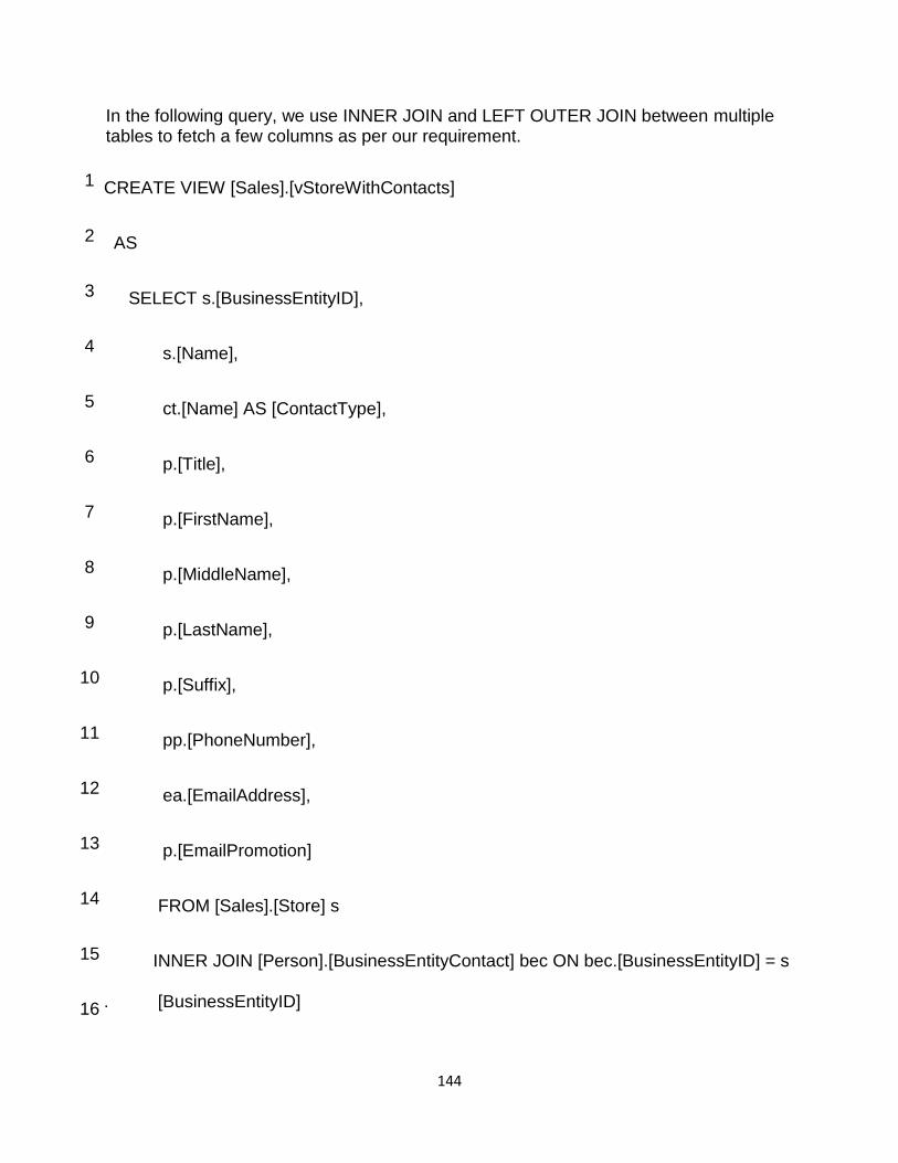
144

In the following query, we use INNER JOIN and LEFT OUTER JOIN between multiple tables to fetch a few columns as per our requirement.

1

2

3

4

5

6

7

8

9

10

11

12

13

14

15

16

CREATE VIEW [Sales].[vStoreWithContacts]

AS

SELECT s.[BusinessEntityID],

s.[Name],

ct.[Name] AS [ContactType],

p.[Title],

p.[FirstName],

p.[MiddleName],

p.[LastName],

p.[Suffix],

pp.[PhoneNumber],

ea.[EmailAddress],

p.[EmailPromotion]

FROM [Sales].[Store] s

INNER JOIN [Person].[BusinessEntityContact] bec ON bec.[BusinessEntityID] = s

. [BusinessEntityID]

145

17

18

19

20

INNER JOIN [Person].[ContactType] ct ON ct.[ContactTypeID] = bec.

[ContactTyp

eID]

INNER JOIN [Person].[Person] p ON p.[BusinessEntityID] = bec.[PersonID]

LEFT OUTER JOIN [Person].[EmailAddress] ea ON ea.[BusinessEntityID] = p.[Bu

sinessEntityID]

LEFT OUTER JOIN [Person].[PersonPhone] pp ON pp.[BusinessEntityID] = p.[Bu

sinessEntityID];

GO

Suppose you need to execute this query very frequently. Using a VIEW, we can simply get the data with a single line of code.

1 select * from [Sales].[vStoreWithContacts]

146

Example 5: SQL VIEW to fetch specific column

In the previous example, we created a VIEW with multiple tables and a few column from those tables. Once we have a view, it is not required to fetch all columns from the view. We can select few columns as well from a VIEW in SQL Server similar to a relational table.

In the following query, we want to get only two columns name and contract type from the view.

1

2

3

SELECT Name,

ContactType

FROM [Sales].[vStoreWithContacts];

Example 6: Use Sp_helptext to retrieve VIEW definition

We can use sp_helptext system stored procedure to get VIEW definition. It returns the complete definition of a SQL VIEW.

For example, let‘s check the view definition for EmployeeRecords VIEW.

We can use SSMS as well to generate the script for a VIEW. Expand database -> Views -> Right click and go to Script view as -> Create To -> New Query Editor Window.

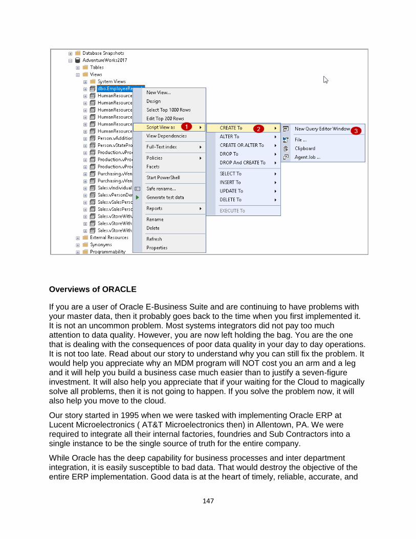
147

Overviews of ORACLE

If you are a user of Oracle E-Business Suite and are continuing to have problems with your master data, then it probably goes back to the time when you first implemented it. It is not an uncommon problem. Most systems integrators did not pay too much attention to data quality. However, you are now left holding the bag. You are the one that is dealing with the consequences of poor data quality in your day to day operations. It is not too late. Read about our story to understand why you can still fix the problem. It would help you appreciate why an MDM program will NOT cost you an arm and a leg and it will help you build a business case much easier than to justify a seven-figure investment. It will also help you appreciate that if your waiting for the Cloud to magically solve all problems, then it is not going to happen. If you solve the problem now, it will also help you move to the cloud.

Our story started in 1995 when we were tasked with implementing Oracle ERP at Lucent Microelectronics ( AT&T Microelectronics then) in Allentown, PA. We were required to integrate all their internal factories, foundries and Sub Contractors into a single instance to be the single source of truth for the entire company.

While Oracle has the deep capability for business processes and inter department integration, it is easily susceptible to bad data. That would destroy the objective of the entire ERP implementation. Good data is at the heart of timely, reliable, accurate, and

148

complete information and is the bedrock of data-oriented decision making. Good Master data, is a prerequisite for good data. To generate good master data, the following attributes are mandatory.

1. Easy User Interface

2. Real time error checking to enforce policies and constraints

3. Approvals to ensure stakeholders signoff

4. No Latency between the time the data is created and its consumption in downstream transactions

5. No gaps between data in the ERP and data in the MDM.

To meet these objectives, we built a custom solution for them and it was for the product domain. Subsequently, when we implemented the same ERP for Sony Semiconductor in Japan, we decided to build a framework that could handle multiple business entities such as Product, Customer, Supplier, GL account, Cost Center, Location, People etc.,

Since Sony Semiconductor went live, many other customers have used Triniti‘s MDM to create and maintain high quality master data. They include Qualcomm, Power Integrations, DSPG and Peregrine Semiconductor.

With Triniti‘s MDM you can achieve the benefits of zero latency enterprise to make faster, and reliable decision making. Armed with error-free transactions in your ERP,CRM, etc, you will be able to avoid pitfalls of not meeting program expectations.

By using Triniti‘s MDM you can achieve the following functionality:

Model your master data for applications other than Oracle and SFDC as well

Model additional complex hierarchies that represent your master data

Set your own policies and constraints, other than that are required by Oracle and SFDC which are already builtin

Validate foreign keys with member applications directly without replicating in the MDM

Do data quality checks

Integrate with other applications in real time using industry standard protocols

Enforce authorship

149

Execute survivorship in member applications

Define required workflows and approvals

Get data quality metrics

Configure 360-degree views of your domains

Summary

Since we have solved the problem, you can leverage our experience and our tools. The integration is 100% reusable and is robust. The backbone is a framework and not a custom solution. It has continued to evolve as technology has evolved, that is illustrated by our ability to integrate with SFDC and demonstrate that we can quickly adapt to the Cloud. This is what enables you to acquire industrial strength MDM capabilities at a very affordable price from us. We also save you considerable time during implementation by reading YOUR configuration and not just configuration based on the VISION database. If you do not solve the problem now, then not only will you continue to bear the consequences of poor data quality, but you will either carry it to the cloud, or will impede your move to the cloud. On the other hand if you do it now, then your move to the cloud will be clean. You would stilll have to worry about MDM being a part of cloud, but if you go with us, we will ensure that we are integrated to your cloud platform as well.

Triniti MDM provides out-of-the-box support for Oracle E-Business suite and SFDC for Product, Customer, Supplier, and GL Chart of accounts structure including GL Account and Cost Center. Check back! We will update our content as we release more domains.

To make your job easier, we also provide the following tools:

1. An ROI Calculator. 2. A Vendor evaluation form.

Data definition and manipulation

DBMS software primarily functions as an interface between the end user and the

database, simultaneously managing the data, the database engine, and the database

schema in order to facilitate the organization and manipulation of data.

Though functions of DBMS vary greatly, general-purpose DBMS features and

capabilities should include: a user accessible catalog describing metadata, DBMS

library management system, data abstraction and independence, data security, logging

and auditing of activity, support for concurrency and transactions, support for

authorization of access, access support from remote locations, DBMS data recovery

support in the event of damage, and enforcement of constraints to ensure the data

follows certain rules.

A database schema design technique that functions to increase clarity in organizing

data is referred to as normalization. Normalization in DBMS modifies an existing

150

schema to minimize redundancy and dependency of data by splitting a large table into

smaller tables and defining the relationship between them. DBMS Output is a built-in

package SQL in DBMS that enables the user to display debugging information and

output, and send messages from subprograms, packages, PL/SQL blocks, and triggers.

Oracle originally developed the DBMS File Transfer package, which provides

procedures to copy a binary file within a database or to transfer a binary file between

databases.

A database management system functions through the use of system commands, first

receiving instructions from a database administrator in DBMS, then instructing the

system accordingly, either to retrieve data, modify data, or load existing data from the

system. Popular DBMS examples include cloud-based database management

systems, in-memory database management systems (IMDBMS), columnar database

management systems (CDBMS), and NoSQL in DBMS.

RDBMS vs DBMS

A relational database management system (RDBMS) refers to a collection of programs

and capabilities that is designed to enable the user to create, update, and administer

a relational database, which is characterized by its structuring of data into logically

independent tables. There are several features that distinguish a Relational DBMS from

a DBMS, including:

Structure: Where data is structured in hierarchical form in a DBMS, data is structured in tabular form in a RDBMS.

User capacity: A RDBMS is capable of operating with multiple users. DBMS can only manage one user at a time.

Software/hardware requirements: A RDBMS has greater software and hardware requirements.

Programs managed: DBMS maintains databases within the computer network and system hard disks. A RDBMS manages the relationships between its incorporated tables of data.

Data capacity: A DBMS is capable of managing small amounts of data and a RDBMS can manage an unlimited amount of data.

Distributed databases: A DBMS does not provide support for distributed databases while a RDBMS does.

ACID implementation: A RDBMS bases the structure of its data on the ACID (Atomicity, Consistency, Isolation, and Durability) model.

151

Difference Between Data and Information in DBMS

Data is raw, unprocessed, unorganized facts that are seemingly random and do not yet

carry any significance or meaning. Information refers to data that has been organized,

interpreted, and contextualized by a human or machine so that it possess relevance and

purpose.

Information is filtered data that has been made systematic and useful, and is considered

to be more reliable and valuable to researchers as proper analysis and refinement has

been conducted. A DBMS is concerned with the manipulation of data in a database.

Difference Between Data Models in DBMS

A data model is an abstract model that organizes elements of data, documents the way

data is stored and retrieved, standardizes how different data elements relate to one

another and to the properties of real-world entities, and designs the responses needed

for information system requirements. There are three main types of DBMS data models:

relational, network, and hierarchical.

Relational data model: Data is organized as logically independent tables. Network data model: All entities are organized in graphical representations. Hierarchical data model: Data is organized into a tree-like structure.

Other data models include entity-relationship, record base, object-oriented, object

relation, semi-structured, associative, context, and flat data models. Database system

architecture in DBMS is categorized as either single tier, in which the DBMS is the only

entity where the user directly sits on the DBMS and uses it, or multi-tier, in which nearly

all components are independent and can be changed independently.

Features of Distributed Database Management System

A distributed database is a collection of related data in multiple interconnected

databases that are logically interrelated, but physically stored across multiple physical

locations. Distributed databases are categorized as either homogeneous, in which all

the physical locations use the same hardware and run the same operating systems and

applications, or heterogeneous, in which each location may have different data,

software, and hardware structures.

A distributed database management system (DDBMS) refers to a centralized

application that functions to create and manipulate distributed databases, synchronize

the database at regular intervals and provide transparent access mechanisms to the

user, ensure universal application of data modifications, maintain data security and

integrity of the database, can be accessed by several users simultaneously, and is used

in applications that process large volumes of data.

152

How is a DBMS Different from a Traditional File System?

A traditional filing system refers to early endeavors to computerize the manual filing

system. File-based systems typically use storage devices such as a CD-ROM or hard

disk to store and organize computer files and the data within with the goal of facilitating

easy access.

A traditional file system is inexpensive, ideal for a small system with smaller quantity of

parts, very low design efforts, isolated data, and has a simple backup system, but is not

secure, has a lack of flexibility and many limitations, and has integrity flaws.

The benefits of DBMS over a traditional file system include: good for large systems,

data-sharable, flexible, has data integrity, and has a complex backup system. DBMS

data security requirements leverage the use of masking, tokenization, encryption,

access control lists, permissions, firewalls, and virtual private networks, making data

storage and querying in DBMS a far more secure option than in a traditional file system.

Does OmniSci Offer a DBMS Solution?

The analytics platform is the solution designed to compensate for the inadequacies of

the relational database management system, working in tandem with various data

processing techniques to address the increasing demands of users in large, data-driven

industries. While so much of today‘s data is now location-enriched, geospatial-specific

processes in GIS tools are becoming too slow for today's data volumes. OmniSci

bridges this divide by making geospatial intelligence (GEOINT) capabilities a first-class

citizen of our accelerated analytics platform.

153

Unit - V

Database Security, Integrity and Control

Security and Integrity threats

In this chapter, we will look into the threats that a database system faces and the measures of control. We will also study cryptography as a security tool.

Database Security and Threats

Data security is an imperative aspect of any database system. It is of particular importance in distributed systems because of large number of users, fragmented and replicated data, multiple sites and distributed control.

Threats in a Database

Availability loss − Availability loss refers to non-availability of database objects by legitimate users.

Integrity loss − Integrity loss occurs when unacceptable operations are performed upon the database either accidentally or maliciously. This may happen while creating, inserting, updating or deleting data. It results in corrupted data leading to incorrect decisions.

Confidentiality loss − Confidentiality loss occurs due to unauthorized or unintentional disclosure of confidential information. It may result in illegal actions, security threats and loss in public confidence.

Measures of Control

The measures of control can be broadly divided into the following categories −

Access Control − Access control includes security mechanisms in a database management system to protect against unauthorized access. A user can gain access to the database after clearing the login process through only valid user accounts. Each user account is password protected.

154

Flow Control − Distributed systems encompass a lot of data flow from one site to another and also within a site. Flow control prevents data from being transferred in such a way that it can be accessed by unauthorized agents. A flow policy lists out the channels through which information can flow. It also defines security classes for data as well as transactions.

Data Encryption − Data encryption refers to coding data when sensitive data is to be communicated over public channels. Even if an unauthorized agent gains access of the data, he cannot understand it since it is in an incomprehensible format.

What is Cryptography?

Cryptography is the science of encoding information before sending via unreliable communication paths so that only an authorized receiver can decode and use it.

The coded message is called cipher text and the original message is called plain text. The process of converting plain text to cipher text by the sender is called encoding or encryption. The process of converting cipher text to plain text by the receiver is called decoding or decryption.

The entire procedure of communicating using cryptography can be illustrated through the following diagram −

155

Conventional Encryption Methods

In conventional cryptography, the encryption and decryption is done using the same secret key. Here, the sender encrypts the message with an encryption algorithm using a copy of the secret key. The encrypted message is then send over public communication channels. On receiving the encrypted message, the receiver decrypts it with a corresponding decryption algorithm using the same secret key.

Security in conventional cryptography depends on two factors −

A sound algorithm which is known to all.

A randomly generated, preferably long secret key known only by the sender and the receiver.

The most famous conventional cryptography algorithm is Data Encryption Standard or DES.

The advantage of this method is its easy applicability. However, the greatest problem of conventional cryptography is sharing the secret key between the communicating parties. The ways to send the key are cumbersome and highly susceptible to eavesdropping.

Public Key Cryptography

In contrast to conventional cryptography, public key cryptography uses two different keys, referred to as public key and the private key. Each user generates the pair of public key and private key. The user then puts the public key in an accessible place. When a sender wants to sends a message, he encrypts it using the public key of the receiver. On receiving the encrypted message, the receiver decrypts it using his private key. Since the private key is not known to anyone but the receiver, no other person who receives the message can decrypt it.

The most popular public key cryptography algorithms are RSA algorithm and Diffie– Hellman algorithm. This method is very secure to send private messages. However, the problem is, it involves a lot of computations and so proves to be inefficient for long messages.

The solution is to use a combination of conventional and public key cryptography. The secret key is encrypted using public key cryptography before sharing between the communicating parties. Then, the message is send using conventional cryptography with the aid of the shared secret key.

Digital Signatures

A Digital Signature (DS) is an authentication technique based on public key cryptography used in e-commerce applications. It associates a unique mark to an

156

individual within the body of his message. This helps others to authenticate valid senders of messages.

Typically, a user‘s digital signature varies from message to message in order to provide security against counterfeiting. The method is as follows −

The sender takes a message, calculates the message digest of the message and signs it digest with a private key.

The sender then appends the signed digest along with the plaintext message.

The message is sent over communication channel.

The receiver removes the appended signed digest and verifies the digest using the corresponding public key.

The receiver then takes the plaintext message and runs it through the same message digest algorithm.

If the results of step 4 and step 5 match, then the receiver knows that the message has integrity and authentic.

Defense mechanism

Database security encompasses a range of security controls designed to protect the Database Management System (DBMS). The types of database security measures your business should use include protecting the underlying infrastructure that houses the database such as the network and servers), securely configuring the DBMS, and the access to the data itself.

Database security controls

Database security encompasses multiple controls, including system hardening, access, DBMS configuration, and security monitoring. These different security controls help to manage the circumventing of security protocols.

System hardening and monitoring

The underlying architecture provides additional access to the DBMS. It is vital that all systems are patched consistently, hardened using known security configuration standards, and monitored for access, including insider threats.

DBMS configuration

It is critical that the DBMS be properly configured and hardened to take advantage of security features and limit privileged access that may cause a misconfiguration of expected security settings. Monitoring the DBMS configuration and ensuring proper change control processes helps ensure that the configuration stays consistent.

157

Authentication

Database security measures include authentication, the process of verifying if a user‘s credentials match those stored in your database, and permitting only authenticated users access to your data, networks, and database platform.

Access

A primary outcome of database security is the effective limitation of access to your data. Access controls authenticate legitimate users and applications, limiting what they can access in your database. Access includes designing and granting appropriate user attributes and roles and limiting administrative privileges.

Database auditing

Monitoring (or auditing) actions as part of a database security protocol delivers centralized oversight of your database. Auditing helps to detect, deter, and reduce the overall impact of unauthorized access to your DBMS.

Backups

A data backup, as part of your database security protocol, makes a copy of your data and stores it on a separate system. This backup allows you to recover lost data that may result from hardware failures, data corruption, theft, hacking, or natural disasters.

Encryption

Database security can include the secure management of encryption keys, protection of the encryption system, management of a secure, off-site encryption backup, and access restriction protocols.

Application security

Database and application security framework measures can help protect against common known attacker exploits that can circumvent access controls, including SQL injection.

Why is database security important?

Safeguarding the data your company collects and manages is of utmost importance. Database security can guard against a compromise of your database, which can lead to

158

financial loss, reputation damage, consumer confidence disintegration, brand erosion, and non-compliance of government and industry regulation.

Database security safeguards defend against a myriad of security threats and can help protect your enterprise from:

Deployment failure

Excessive privileges

Privilege abuse

Platform vulnerabilities

Unmanaged sensitive data

Backup data exposure Weak authentication

Database injection attacks

Auditing and Control

A simple definition for what a database management system (DBMS) is, would be that

it is a complex set of software programs that control the organization, storage and

retrieval of data in a database. It also controls the security and integrity of the

database.

This article will not attempt to give a detailed explanation of database technology, rather it will serve to introduce the IT auditor to some of the concepts that will be necessary to be understood and performed to support an audit of a DBMS.

But first, in order to understand DBMS there is some database terminology and definitions you will need to understand:

Concurrency Control – Refers to the class of controls used in database management systems (DBMS) to ensure that transactions are processed in an atomic, consistent, isolated and durable manner (ACID). This implies that only serial and recoverable schedules are permitted, and that committed transactions are not discarded when undoing aborted transactions.

Data Structure – The relationships among files in a database and among data items within each file.

Database – A stored collection of related data needed by organizations and individuals to meet their information processing and retrieval requirements.

159

Database Administrator (DBA) – An individual or department responsible for the security and information classification of the shared data stored on a database system. This responsibility includes the design, definition and maintenance of the database.

Database Specifications – These are the requirements for establishing a database application. They include field definitions, field requirements, and reporting requirements for the individual information in the database.

Foreign Key – A foreign key is a value that represents a reference to a tuple (a row in a table) containing the matching candidate key value (in the relational theory it would be a candidate key, but in real DBMS implementations it is always the primary key). The problem of ensuring that the database does not include any invalid foreign key values is therefore known as the referential integrity problem. The constraint that values of a given foreign key must match values of the corresponding candidate key is known as a referential constraint. The relation (table) that contains the foreign key is referred as the referencing relation and the relations that contain the corresponding candidate key as the referenced relation or target relation.

Normalization – The elimination of redundant data.

Repository – The central database that stores and organizes data.

Transaction log – A manual or automated log of all updates to data files and databases.

Tuple – A tuple is a row in a database table.

When we speak about Database Management Systems (DBMS), there are three basic types:

Hierarchical – a database structured in a tree/root or parent/child relationship. Each parent can have many children; however, each child may have only one parent.

Network – the basic data modeling construct is called a set. A set is formed by an owner record type, a member record type and a name. A member record type can have that role in more than one set, so a multi-owner relationship is allowed. An owner record type can also be a member or owner in another set. Usually, a set defines a 1:N relationship, although one-to-one (1:1) is permitted. A disadvantage of the network model is that such structures can be extremely complex and difficult to comprehend, modify or reconstruct in case of failure.

Relational – This model is based on the set theory and relational calculations. A relational database allows the definition of data structures, storage/retrieval operations and integrity constraints. In such a database the data and relationships among these data are organized in tables. A table is a collection of rows, also known as tuples, and each tuple in a table contains the same number of columns. Columns, called domains or attributes, correspond to fields. Tuples are equal to records in a conventional file structure.

Relational tables have the following characteristics:

160

Values are atomic

Each row is unique

Column values are of the same kind

The sequence of columns is insignificant

The sequence of rows is insignificant

Each column has a unique name

Some of the advantages of the relational model over the hierarchical and network model are that it is easier:

For users to understand and implement a physical database system

To convert from other database structures

To implement projection and join operations

To create new relations for applications

To implement access control over sensitive data

To modify the data base

When auditing the controls of a database, the auditor would check to see that the following controls have been implemented and maintained to ensure database integrity and availability:

Definition standards

Data backup and recovery procedures

Access controls

Only authorized personnel can update the database

Controls to handle concurrent access problems such as multiple users trying to update the same record at the same time

Controls to ensure the accuracy, completeness and consistency of data elements and relationships.

Checkpoints to minimize data loss

Database re-organizations

Monitoring database performance

Capacity planning

Who can access the database without going through the application?

When we speak of who can access the database, we have already identified one of the major audit concerns and that is what access does the DBA have? As everyone knows the DBA basically has the ―keys to the kingdom‖ and can do (read, write,

161

change, delete) anything. What you have to make sure of is that someone is watching. Someone is monitoring (logging) the actions the DBA takes. And the DBA, doesn‘t have the ability to de-activate the log nor do they have access to the log.

It goes without saying that Access Control is the number one issue with database management systems. That being said let‘s not forget to audit disaster recovery and restoration, patch management, change management, incident logging and all the other issues an auditor should look for.

There is another issue that auditors need to deal with when auditing DBMS and that is to perform some type of data integrity testing. Data integrity testing is a set of substantive tests (NOTE: Substantive not Compliance testing) that examines accuracy, completeness, consistency and authorization of data presently held in a system. There are two common types of data integrity tests; relational and referential. Relational integrity tests are performed at the data element and record-based levels. It is enforced through data validation routines built into the application or by defining the input condition constraints and data characteristics at the table definition in the database stage. Sometimes it is a combination of both.

Referential integrity test define existence relationships between entities in different tables of a database that needs to be maintained by the DBMS. Referential integrity checks involve ensuring that all references to a primary key from another table actually exist in their original table.

With respect to data integrity in online transaction processing systems there are four online data integrity requirements known collectively as the ACID principle. For those of you that are old enough to remember ACID, congratulations, your brain isn‘t completed fried.

The ―A‖ stands for atomicity and from a user‘s perspective, a transaction is either completed in its entirety or not at all.

The ―C‖ stands for consistency. Basically, all integrity conditions in the database are maintained with each transaction, taking the database from one consistent state into another consistent state.

The ―I‖ stands for isolation. Each transaction is isolated from other transactions and hence each transaction only accesses data that are part of a consistent database state.

The ―D‖ stands for durability. If a transaction has been reported back to a user as complete, the resulting changes to the database survive subsequent hardware of software failures.

As a parting comment, I would be remiss, if I didn‘t mention how the database was populated in a test environment. As many times as I have audited databases, I have

162

found that the production environment was being copied to the test environment to ensure an accurate copy so that changes would not fail once they were moved to production. At least that was the logical in the client‘s explanation. What they fail to realize is that the security controls in test are significantly weaker that they are in production and yet there is a mirror unprotected copy sitting there for all to see.

At least as an auditor, you should recommend that the data be sanitized before being used in test.

I hope you‘ve enjoyed this brief overview of DBMS and have an appreciation of some things you might check as an auditor.

Recent trends in DBMS

Concepts in database management hardly fall in the category of come-and-go, as the cost of shifting between technical approaches overwhelms producers, managers, and designers. However, there are several trends in database management, and knowing how to take advantage of them will benefit your organization. Following are the some of the current trends:

1. Databases that bridge SQL/NoSQL

The latest trends in database products are those that don‘t simply embrace a single database structure. Instead, the databases bridge SQL and NoSQL, giving users the best capabilities offered by both. This includes products that allow users to access a NoSQL database in the same way as a relational database, for example.

2. Databases in the cloud/Platform as a Service As developers continue pushing their enterprises to the cloud, organizations are carefully weighing the trade-offs associated with public versus private. Developers are also determining how to combine cloud services with existing applications and infrastructure. Providers of cloud service offer many options to database administrators. Making the move towards the cloud doesn‘t mean changing organizational priorities, but finding products and services that help your group meet its goals.

3. Automated management Automating database management is another emerging trend. The set of such techniques and tools intend to simplify maintenance, patching, provisioning, updates and upgrades — even project workflow. However, the trend may have limited usefulness since database management frequently needs human intervention.

4. An increased focus on security While not exactly a trend given the constant focus on data security, recent ongoing retail database breaches among US-based organizations show with ample clarity the importance for database administrators to work hand-in-hand with their IT security colleagues to ensure all enterprise data remains safe. Any organization that stores data is vulnerable. Database administrators must also work with the security team to eliminate potential internal weaknesses that could make data vulnerable. These could include issues

163

related to network privileges, even hardware or software misconfigurations that could be misused, resulting in data leaks.

5. In-memory databases Within the data warehousing community there are similar questions about columnar versus row-based relational tables; the rise of in-memory databases, the use of flash or solid-state disks (which also applies within transaction processing), clustered versus no-clustered solutions and so on.

6. Big Data To be clear, big data does not necessarily mean lots of data. What it really refers to is the ability to process any type of data: what is typically referred to as semi-structured and unstructured data as well as structured data. Current thinking is that these will typically live alongside conventional solutions as separate technologies, at least in large organisations, but this will not always be the case.

Integrating Trends

Projects involving databases should not be viewed and appreciated solely on how they adhere to these trends. Ideally, each tool or process available should merge in some meaningful way with existing operations. It is important to look of these trends as items that can coincide: enhancing security and moving to the cloud coexist?

Distributed and Deductive Database

Distributed Database:- This chapter introduces the concept of DDBMS. In a distributed database, there are a number of databases that may be geographically distributed all over the world. A distributed DBMS manages the distributed database in a manner so that it appears as one single database to users. In the later part of the chapter, we go on to study the factors that lead to distributed databases, its advantages and disadvantages.

A distributed database is a collection of multiple interconnected databases, which are spread physically across various locations that communicate via a computer network.

Features

Databases in the collection are logically interrelated with each other. Often they represent a single logical database.

Data is physically stored across multiple sites. Data in each site can be managed by a DBMS independent of the other sites.

The processors in the sites are connected via a network. They do not have any multiprocessor configuration.

A distributed database is not a loosely connected file system.

164

A distributed database incorporates transaction processing, but it is not synonymous with a transaction processing system.

Distributed Database Management System

A distributed database management system (DDBMS) is a centralized software system that manages a distributed database in a manner as if it were all stored in a single location.

Features

It is used to create, retrieve, update and delete distributed databases.

It synchronizes the database periodically and provides access mechanisms by the virtue of which the distribution becomes transparent to the users.

It ensures that the data modified at any site is universally updated.

It is used in application areas where large volumes of data are processed and accessed by numerous users simultaneously.

It is designed for heterogeneous database platforms.

It maintains confidentiality and data integrity of the databases.

Factors Encouraging DDBMS

The following factors encourage moving over to DDBMS −

Distributed Nature of Organizational Units − Most organizations in the current times are subdivided into multiple units that are physically distributed over the globe. Each unit requires its own set of local data. Thus, the overall database of the organization becomes distributed.

Need for Sharing of Data − The multiple organizational units often need to communicate with each other and share their data and resources. This demands common databases or replicated databases that should be used in a synchronized manner.

Support for Both OLTP and OLAP − Online Transaction Processing (OLTP) and Online Analytical Processing (OLAP) work upon diversified systems which may have common data. Distributed database systems aid both these processing by providing synchronized data.

Database Recovery − One of the common techniques used in DDBMS is replication of data across

165

different sites. Replication of data automatically helps in data recovery if database in any site is damaged. Users can access data from other sites while the damaged site is being reconstructed. Thus, database failure may become almost inconspicuous to users.

Support for Multiple Application Software − Most organizations use a variety of application software each with its specific database support. DDBMS provides a uniform functionality for using the same data among different platforms.

Advantages of Distributed Databases

Following are the advantages of distributed databases over centralized databases.

Modular Development − If the system needs to be expanded to new locations or new units, in centralized database systems, the action requires substantial efforts and disruption in the existing functioning. However, in distributed databases, the work simply requires adding new computers and local data to the new site and finally connecting them to the distributed system, with no interruption in current functions.

More Reliable − In case of database failures, the total system of centralized databases comes to a halt. However, in distributed systems, when a component fails, the functioning of the system continues may be at a reduced performance. Hence DDBMS is more reliable.

Better Response − If data is distributed in an efficient manner, then user requests can be met from local data itself, thus providing faster response. On the other hand, in centralized systems, all queries have to pass through the central computer for processing, which increases the response time.

Lower Communication Cost − In distributed database systems, if data is located locally where it is mostly used, then the communication costs for data manipulation can be minimized. This is not feasible in centralized systems.

Adversities of Distributed Databases

Following are some of the adversities associated with distributed databases.

Need for complex and expensive software −

166

DDBMS demands complex and often expensive software to provide data transparency and co-ordination across the several sites.

Processing overhead − Even simple operations may require a large number of communications and additional calculations to provide uniformity in data across the sites.

Data integrity − The need for updating data in multiple sites pose problems of data integrity.

Overheads for improper data distribution − Responsiveness of queries is largely dependent upon proper data distribution. Improper data distribution often leads to very slow response to user requests.

Deductive Database:- A deductive database is a finite collection of facts and rules. By applying the rules of a deductive database to the facts in the database, it is possible to infer additional facts, i.e. facts that are implicitly true but are not explicitly represented in the database.

This paper is a brief introduction to deductive databases. In the first section, we talk about traditional databases, i.e. sets of simple facts. After that, we introduce logic programs, i.e. sets of rules. We then show how to use rules in defining views of a database, in writing constraints on the database, and in defining updates to the database. We close with a brief discussion of special, built-in functions and relations.

2. Databases

When we think about the world, we usually think in terms of objects and relationships among these objects. Objects include things like people and offices and buildings. Relationships include things like the parenthood, ancestry, office assignments, office locations, and so forth.

In sentential databases, we encode each instance of a relationship in the form of a sentence consisting of a relation constant representing the relationship and some terms representing the objects involved in the instance.

The vocabulary of a database is a collection of object constants, function constants, and relation constants. Each function constant and relation constant has an associated arity, i.e. the number of objects involved in any instance of the corresponding function or relation.

167

A term is either a symbol or a functional term. A functional term is an expression consisting of an n-ary function constant and n terms. In what follows, we write functional terms in traditional mathematical notation - the function followed by its arguments enclosed in parentheses and separated by commas. For example, if f is a binary function constant and if a and b are object constants, then f(a,a) and f(a,b) and f(b,a) and f(b,b) are all functional terms. Functional terms can be nested within other functional terms. For example, if f(a,b) is a functional term, then so is f(f(a,b),b).

A datum is an expression formed from an n-ary relation constant and n terms. We write data in mathematical notation. For example, we might write parent(art,bob) to express the fact that Art is the parent of Bob.

A dataset is any set of data that can be formed from the vocabulary of a database. Intuitively, we can think of the data in a dataset as the facts that we believe to be true in the world; data that are not in the dataset are assumed to be false.

As an example of these concepts, consider a small interpersonal database. The objects in this case are people. The relationships specify properties of these people and their interrelationships.

In our example, we use the binary relation constant parent to specify that one person is a parent of another. The sentences below constitute a database describing six instances of the parent relation. The person named art is a parent of the person named bob; art is also a parent of bea, and so forth.

parent(art,bob)

parent(art,bea)

parent(bob,carl)

parent(bea,coe)

parent(carl,daisy)

parent(carl,daniel)

The adult relation is unary relation, i.e. a simple property of a person, not a relationship other people. Everyone in our database is an adult except for daisy and daniel.

adult(art)

168

adult(bob)

adult(bea)

adult(carl)

adult(coe)

We can express gender with two unary relation constants male and female. The following data expresses the genders of all of the people in our database. Note that, in principle, we need only one relation here, since one gender is the complement of the other. However, representing both allows us to enumerate instances of both gender equally efficiently, which can be useful in certain applications.

male(art)

female(bea)

male(bob)

female(coe)

male(cal)

female(daisy)

male(daniel)

As an example of a ternary relation, consider the data shown below. Here, we use prefers to represent the fact that the first person likes the second person more than the third person. For example, the first sentence says that Art prefers bea to bob; the second sentence says that carl prefers daisy to daniel.

prefers(art,bea,bob)

prefers(carl,daisy,daniel)

Note that the order of arguments in such sentences is arbitrary. Given the meaning of the prefers relation in our example, the first argument denotes the subject, the second argument is the person who is preferred, and the third argument denotes the person who is less preferred. We could equally well have interpreted the arguments in other orders. The important thing is consistency - once we choose to interpret the arguments in one way, we must stick to that interpretation everywhere.

169

3. Logic Programs

The rules in a deductive database are often called a logic program. The language of logic programs includes the language of databases but provides additional expressive features.

One key difference is the inclusion of a new type of symbol, called a variable. Variables allow us to state relationships among objects without explicitly naming those objects. In what follows, we use individual capital letters as variables, e.g. X, Y, Z.

In the context of logic programs, a term is defined as an object constant, a variable, or a functional term, i.e. an expression consisting of an n-ary function constant and n simpler terms.

An atom in a logic program is analogous to a datum in a database except that the constituent terms may include variables.

A literal is either an atom or a negation of an atom (i.e. an expression stating that the atom is false). A simple atom is called a positive literal, The negation of an atom is called a negative literal. In what follows, we write negative literals using the negation sign ~. For example, if p(a,b) is an atom, then ~p(a,b) denotes the negation of this atom.

A rule is an expression consisting of a distinguished atom, called the head and a conjunction of zero or more literals, called the body. The literals in the body are called subgoals. In what follows, we write rules as in the example shown below. Here, r(X,Y) is the head, p(X,Y) & ~q(Y) is the body; and p(X,Y) and ~q(Y) are subgoals.

r(X,Y) :- p(X,Y) & ~q(Y)

Semantically, a rule is something like a reverse implication. It is a statement that the conclusion of the rule is true whenever the conditions are true. For example, the rule above states that r is true of any object X and any object Y if p is true of X and Y and q is not true of Y. For example, if we know p(a,b) and we know that q(b) is false, then, using this rule, we can conclude that r(a,b) must be true.

Exercise: Click here to test your understanding of rule syntax.

A logic program is a finite set of atoms and rules as just defined. In order to simplify our definitions and analysis, we occasionally talk about infinite sets of rules. While these sets are useful, they are not themselves logic programs.

170

Unfortunately, the language of rules, as defined so far, allows for logic programs with some unpleasant properties. To avoid programs of this sort, it is common in deductive databases to add a couple of restrictions that together eliminate these problems.

The first restriction is safety. A rule in a logic program is safe if and only if every variable that appears in the head or in any negative literal in the body also appears in at least one positive literal in the body. A logic program is safe if and only if every rule in the program is safe.

All of the examples above are safe. By contrast, the two rules shown below are not safe. The first rule is not safe because the variable Z appears in the head but does not appear in any positive subgoal. The second rule is not safe because the variable Z appears in a negative subgoal but not in any positive subgoal.

s(X,Y,Z) :- p(X,Y)

t(X,Y) :- p(X,Y) & ~q(Y,Z)

To see why safety is matters in the case of the first rule, suppose we had a database in which p(a,b) is true. Then, the body of the first rule is satisfied if we let X be a and Y be b. In this case, we can conclude that every corresponding instance of the head is true. But what should we substitute for Z? Intuitively, we could put anything there; but there could be infinitely many possibilities. For example, we could write any number there. While this is conceptually okay, it is practically problematic.

To see why safety matters in the second rule, suppose we had a database with just two facts, viz. p(a,b) and q(b,c). In this case, if we let X be a and Y be b and Z be anything other than c, then both subgoals true, and we can conclude t(a,b). The main problem with this is that many people incorrectly interpret that negation as meaning there is no Z for which q(Y,Z) is true, whereas the correct reading is that q(Y,Z) needs to be false for just one binding of Z. As we will see in our examples below, there is a simple way of expressing this other meaning without writing unsafe rules.

In logic programming, these problems are avoided by requiring all rules to be safe. While this does restrict what one can say, the good news is that it is usually possible to ensure safety by adding additional subgoals to rules to ensure that the restrictions are satisfied.

Exercise: Click here to test your understanding of the concept of safety.

The second restriction is called stratified negation. It is essential in order to avoid ambiguities. Unfortunately, it is a little more difficult to understand than safety.

The dependency graph for a logic program is a directed graph with two type of arcs, positive and negative. The nodes in the dependency graph for a program

171

represent the relations in the program. There is a positive arc in the graph from one node to another if and only if the former node appears in a positive subgoal of a rule in which the latter node appears in the head. There is a negative arc from one node to another if and only if the former node appears in a negative subgoal of a rule in which the latter node appears in the head.

As an example, consider the following logic program. r(X,Y) is true if p(X,Y) and q(Y) are true. s(X,Y) is true if r(X,Y) is true and s(Y,X) is false.

r(X,Y) :- p(X,Y) & q(Y)

s(X,Y) :- r(X,Y) & ~s(Y,X)

The dependency graph for this program contains nodes for p, q, r, and s. Due to the first rule, there is a positive arc from p to r and a positive arc from q to r. Due to the second rule, there is a positive arc from r to s and a negative arc from s to itself.

A negation in a logic program is said to be stratified with respect to negation if and only if there is no negative arc in any cycle in the dependency graph. The logic program just shown is not stratified with respect to negation because there is a cycle involving a negative arc.

The problem with unstratified logic programs is that there is a potential ambiguity. As an example, consider the program above and assume we had a database containing p(a,b), p(b,a), q(a), and q(b). From these facts we can conclude r(a,b) and r(b,a) are both true. So far so good. But what can we say about s? If we take s(a,b) to be true and s(b,a) to be false, then the second rule is satisfied. If we take s(a,b) to be false and s(b,a) to be true, then the second rule is again satisfied. We can also take them both to be true. The upshot is that there is ambiguity about s. By concentrating exclusively on programs that are stratified with respect to negation, we avoid such ambiguities.

Exercise: Click here to test your understanding of the concept of stratified negation.

It is common in logic programming to require that all logic programs be both safe and stratified with respect to negation. The restrictions are easy to satisfy in most applications; and, by obeying these restrictions, we ensure that our logic programs produce finite, unambiguous answers for all questions.

4. View Definitions

The principle use of rules is to define new relations in terms of existing relations. The new relations defined in this way are often called view relations (or simply views) to distinguish them from base relations, which are defined by explicit enumeration of instances.

172

To illustrate the use of rules in defining views, consider once again the world of interpersonal relations. Starting with the base relations, we can define various interesting view relations.

As an example, consider the sentences shown below. The first sentence defines the father relation in terms of parent and male. The second sentence defines mother in terms of parent and female.

father(X,Y) :- parent(X,Y) & male(X)

mother(X,Y) :- parent(X,Y) & female(X)

The rule below defines the grandparent relation in terms of the parent relation. A person X is the grandparent of a person Z if X is the parent of a person Y and Y is the parent of Z. The variable Y here is a thread variable that connects the first subgoal to the second but does not itself appear in the head of the rule.

grandparent(X,Z) :- parent(X,Y) & parent(Y,Z)

Note that the same relation can appear in the head of more than one rule. For example, the person relation is true of a person Y if there is an X such that X is the parent of Y or if Y is the parent of some person Z. Note that in this case the conditions are disjunctive (at least one must be true), whereas the conditions in the grandfather case are conjunctive (both must be true).

person(X) :- parent(X,Y)

person(Y) :- parent(X,Y)

A person X is an ancestor of a person Z if X is the parent of Z or if there is a person Y such that X is an ancestor of and Y is an ancestor of Z. This example shows that is possible for a relation to appear in its own definition. (But recall our discussion of stratification for a restriction on this capability.)

ancestor(X,Y) :- parent(X,Y)

ancestor(X,Z) :- ancestor(X,Y) & ancestor(Y,Z)

A childless person is one who has no children. We can define the property of being childless with the rules shown below. The first rule states that a person X is childless

173

if X is a person and it is not the case that X is a parent. The second rule says that isparent is true of X if X is the parent of some person Y.

childless(X) :- person(X) & ~isparent(X,Y)

isparent(X) :- parent(X,Y)

Note the use of the helper relation isparent here. It is tempting to write the childless rule as childless(X) :- person(X) & ~parent(X,Y). However, this would be wrong. This would define X to be childless if X is a person and there is some Y such that X is ~parent(X,Y) is true. But we really want to say that ~parent(X,Y) holds for all Y. Defining isparent and using its negation in the definition of childless allows us to express this universal quantification.

5. Errors and Warnings

In our development thus far, we have assumed that the extension of an n-ary relation may be any set of n-tuples from the domain. This is rarely the case. Often, there are constraints that limit the set of possibilities. For example, a person cannot be his own parent. In some cases, constraints involve multiple relations. For example, all parents are adults; in other words, if an entity appears in the first column of the parent relation, it must also appear as an entry in the adult relation.

In many database texts, constraints are written in direct form - by writing rules that say, in effect, that if certain things are true in an extension, then other things must also be true. The inclusion dependency mentioned above is an example - if an entity appears in the first column of the parent relation, it must also appear as an entry in the adult relation.

In what follows, we use a slightly less direct approach - we encode limitations by writing rules that say when a database is not well-formed. We simply invent a new 0-ary relation, here called illegal, and define it to be true in any extension that does not satisfy our constraints.

This approach works particularly well for consistency constraints like the one stating that a person cannot be his own parent.

illegal :- parent(X,X)

It also works well for mutual exclusion constraints like the one below, which states that a person cannot be in both the male and the female relations.

illegal :- male(X) & female(X)

Using this technique, we can also write the inclusion dependency mentioned earlier. There is an error if an entity is in the first column of the parent relation and it does not occur in the adult relation.

174

illegal :- parent(X,Y) & ~adult(X)

Database management systems can use such constraints in a variety of ways. They can be used to optimize the processing of queries. They can also be used to check that updates do not lead to unacceptable extensions.

6. Updates

In updating a database, a user specifies a sentence to add to a database or a sentences to delete. In some cases, the user can group several changes of this sort in a single, so-called, atomic transaction. If the result of executing the transaction satisfies the constraints, the update is performed; otherwise it is rejected.

Unfortunately, if a user forgets to include an addition or deletion required by the constraints, this can lead to errors. In order to simplify the update process for the user, some database systems provide the administrator the ability to write update rules, i.e. rules that are executed by the system to augment a specified transaction with the additions and deletions necessary to avoid errors. In what follows, we show one way that this can be done

Our update language includes four special operators - pluss, minus, pos, and neg. pluss takes a sentence as argument and is true if and only if the user specifies that sentence as an addition in a transaction. minus takes a sentence as argument and is true if and only if the user specifies that sentence as an addition in a transaction. pos takes a sentence as argument and is true if and only if the system concludes that the specified sentence should be added to the database. neg takes a sentence as argument and is true if and only if the system concludes that the specified sentence should be added to the database. Update rules are rules that define pos and neg in terms of pluss and minus and the current state of the database.

As an example of this mechanism in action, consider the rules shown below. The first dictates that the system remove a sentence of the form male(X) whenever the user adds a sentence of the form female(X). The second rule is analogous to the first with male and female reversed. Together, these two rules enforce the mutual exclusion on male and female.

neg(male(X)) :- pluss(female(X))

neg(female(X)) :- pluss(male(X))

Similarly, we can enforce the inclusion dependency on parent and adult by writing the following rule. If the user adds a sentence of the form parent(X,Y), then the system also adds a sentence of the form adult(X).

175

pos(adult(X)) :- pluss(parent(X,Y))

Another use of this update mechanism is to maintain materialized views. (A materialized view is a defined relation that is stored explicitly in the database, usually to save recomputation.)

Suppose, for example, we were to materialize the father relation defined earlier. Then we could write the update rules to maintain this materialized view. According to the first rule, the system should add a sentence of the form father(X,Y) whenever the user adds parent(X,Y) and male(X) is know to be true and the user does not delete that fact. The other rules cover the other cases.

pos(father(X,Y)) :- pluss(parent(X,Y)) & male(X) & ~minus(male(X))

pos(father(X,Y)) :- parent(X,Y) & pluss(male(X)) & ~minus(parent(X,Y))

pos(father(X,Y)) :- pluss(parent(X,Y)) & pluss(male(X))

neg(father(X,Y)) :- minus(parent(X,Y))

neg(father(X,Y)) :- minus(male(X))

Note that not all constraints can be enforced using update rules. For example, if a user suggests adding the sentence parent(art,art) to the database in our interpersonal relations example, there is nothing the system can do to repair this error except to reject the transaction. In some cases, there is no way to make a repair unambiguously; more information is needed from the user. For example, we might have a constraint that every person is in either the male or the female relation. If the user specifies a parent fact involving a new person but does not specify the gender of that person, there is no way for the system to decide that gender for itself.

7. Special Relations

In practical logic programming languages, it is common to "build in" commonly used concepts. These typically include arithmetic functions (such as +, *, max, min), string functions (such as concatenation), comparison operators (such as < and >), and equality (=). It is also common to include aggregate operators, such as countofall, avgofall sumofall, and so forth.

In many practical logic programming languages, mathematical functions are represented as relations. For example, the the binary addition operator + is often represented by the the ternary relation constant plus. For example, the following rule

176

defines the combined age of two people. The combined age of X and Y is S if the age of X is M and the age of Y is N and S is the result of adding M andN.

combinedage(X,Y,S) :- age(X,M) & age(Y,N) & plus(M,N,S)

Similarly, aggregate operators are typically represented as relations. For example the following rule defines the number of a person's grandchildren using the countofall relation in this way. N is the number of grandchildren of X if N is the count of all Z such that X is the grandparent of Z.

grandchildren(X,N) :- person(X) & countofall(Z,grandparent(X,Z),N)

In logic programming languages that provide such built-in concepts, there are usually syntactic restrictions on their use. For example, if a rule contains a subgoal with a comparison relation, then every variable that occurs in that subgoal must occur in at least one positive literal in the body and that occurrence must precede the subgoal with the comparison relation. If a rule mentions an arithmetic function, then any variable that occurs in all but the last position of that subgoal must occur in at least one positive literal in the body and that occurrence must precede the subgoal with the arithmetic relation.