Data Augmentation of Visual Rhythms using Symmetric ... · Tacon, Hemerson Aparecido da Costa. Data...
89
UNIVERSIDADE FEDERAL DE JUIZ DE FORA INSTITUTO DE CI ˆ ENCIAS EXATAS P ´ OS-GRADUA ¸ C ˜ AO EM CI ˆ ENCIA DA COMPUTA¸ C ˜ AO Hemerson Aparecido da Costa Tacon Data Augmentation of Visual Rhythms using Symmetric Extension for Deep Learning Video Based Human Action Recognition Juiz de Fora 2019
Transcript of Data Augmentation of Visual Rhythms using Symmetric ... · Tacon, Hemerson Aparecido da Costa. Data...

UNIVERSIDADE FEDERAL DE JUIZ DE FORA
INSTITUTO DE CIENCIAS EXATAS
POS-GRADUACAO EM CIENCIA DA COMPUTACAO
Hemerson Aparecido da Costa Tacon
Data Augmentation of Visual Rhythms using
Symmetric Extension for Deep Learning Video Based
Human Action Recognition
Juiz de Fora
2019

UNIVERSIDADE FEDERAL DE JUIZ DE FORA
INSTITUTO DE CIENCIAS EXATAS
POS-GRADUACAO EM CIENCIA DA COMPUTACAO
Hemerson Aparecido da Costa Tacon
Data Augmentation of Visual Rhythms using
Symmetric Extension for Deep Learning Video Based
Human Action Recognition
Dissertacao apresentada ao Programa dePos-Graduacao em Ciencia da Computacao,do Instituto de Ciencias Exatas daUniversidade Federal de Juiz de Fora comorequisito parcial para obtencao do tıtulo deMestre em Ciencia da Computacao.
Orientador: Marcelo Bernardes Vieira
Juiz de Fora
2019

Hemerson Aparecido da Costa Tacon
Data Augmentation of Visual Rhythms using Symmetric
Extension for Deep Learning Video Based Human Action
Recognition
Dissertacao apresentada ao Programa dePos-Graduacao em Ciencia da Computacao,do Instituto de Ciencias Exatas daUniversidade Federal de Juiz de Fora comorequisito parcial para obtencao do tıtulo deMestre em Ciencia da Computacao.
Aprovada em 11 de Junho de 2019.
BANCA EXAMINADORA
Prof. D.Sc. Marcelo Bernardes Vieira - OrientadorUniversidade Federal de Juiz de Fora
Prof. D.Sc. Saulo Moraes VillelaUniversidade Federal de Juiz de Fora
Prof. D.Sc. Helio PedriniUniversidade Estadual de Campinas

Ficha catalográfica elaborada através do programa de geração automática da Biblioteca Universitária da UFJF,
com os dados fornecidos pelo(a) autor(a)
Tacon, Hemerson Aparecido da Costa. Data augmentation of visual rhythms using symmetric extensionfor deep learning video based human action recognition / HemersonAparecido da Costa Tacon. -- 2019. 88 f. : il.
Orientador: Marcelo Bernardes Vieira Dissertação (mestrado acadêmico) - Universidade Federal deJuiz de Fora, ICE/Engenharia. Programa de Pós-Graduação emCiência da Computação, 2019.
1. Deep Learning. 2. Human Action Recognition. 3. DataAugmentation. 4. Visual Rhythm. 5. Video analysis. I. Vieira, MarceloBernardes, orient. II. Título.

AGRADECIMENTOS
Primeiramente, eu gostaria de agradecer a minha famılia que sempre incentivou meus
estudos durante toda essa jornada, e por todo o esforco empenhado em minha educacao e
criacao. Agradeco tambem pela compreensao nos momentos em que nao pude estar com
voces em minha cidade natal, e tambem nos momentos em que eu estava la mas nao podia
dar muita atencao, pois estava ocupado com afazares academicos.
Sou grato tambem a todos os professores do DCC e do PGCC que, de alguma forma,
contribuıram na minha formacao, e tambem pelos ensinamentos passados durante todos
esses anos de graduacao e de mestrado. Em especial, agradeco ao professor Marcelo
Bernardes pela ideia de tema de pesquisa e pela orientacao. Agradeco tambem a todos
os colegas e amigos da UFJF pelos varios momentos de conversa, risadas e troca de
ideias durante essa jornada. Agradeco principalmente aos meus parceiros de GCG e de
mestrado, Andre e Hugo, com quais compartilhei incertezas, frustracoes, codigos, inumeras
caronas e tambem cada resultado positivo durante essa nossa empreitada de aprender Deep
Learning praticamente sozinhos. Agradeco tambem a colaboracao com o pessoal do LIV
na Unicamp, e em especial a Helena pela imensuravel ajuda executando meus scripts em
algumas maquinas da Unicamp e tambem pela troca de ideias.
Agradeco aos funcionarios da UFJF e do PGCC pelo suporte. Agradeco a CAPES
pelo apoio financeiro sem o qual eu nao teria conseguido realizar este mestrado. Agradeco
tambem a NVIDIA pela doacao de placas de vıdeo sem as quais eu teria conseguido
executar apenas uma pequena fracao dos milhares (nao estou exagerando) de experimentos
que realizei.
Finalmente, agradeco a Dalila. So voce tem nocao do real esforco que foi empenhado
durante este mestrado e esteve do meu lado durante toda essa caminhada, nao me deixando
desanimar, sendo meu porto seguro. Muito obrigado!

“Artificial Intelligence is the new
electricity.” Andrew Ng.

RESUMO
Nos ultimos anos, avancos significativos foram alcancados no problema de classificacao
de imagens devido ao aprimoramentos dos modelos de Aprendizagem Profunda. Entre-
tanto, no que diz respeito ao Reconhecimento de Acoes Humanas, ainda existe muito
espaco para melhorias. Uma forma de melhorar o desempenho de tais modelos e atraves
do aumento de dados. Dessa forma propomos, como aumento de dados, o uso de multi-
plos recortes do Ritmo Visual, simetricamente estendidos no tempo e separados por uma
distancia fixa. Propomos ainda utilizar uma nova forma de extracao do Ritmo Visual, o
Ritmo Visual Ponderado. Este metodo propoe reforcar os padroes de movimento pesando
os aspectos mais proximos de uma posicao especıfica no vıdeo na qual julgamos que a acao
tenha maior probabilidade de ocorrer. O metodo final consiste na replicacao do Ritmo
Visual Ponderado concatenando quantas copias forem necessarias ao longo da dimensao
temporal, tendo as copias pares invertidas horizontalmente. Esse metodo torna possıvel
a extracao de recortes que correspondam ao tamanho de entrada fixo da Rede Neural
Convolucional utilizada, bem como a preservacao da taxa de amostragem do vıdeo, o
que e crucial para nao distorcer a velocidade das acoes. Nao obstante, os varios recortes
garantem que toda extensao espacial e temporal do Ritmo Visual seja contemplada. Com
o objetivo de avaliar nosso metodo, empregamos uma estrategia multi-fluxo. Essa estrate-
gia consiste na combinacao de informacoes extraıdas a partir dos frames RGB dos vıdeos,
do Fluxo Otico, e dos Ritmos Visuais Simetricamente Estendidos horizontal e vertical.
Nosso metodo resultou em taxas de acuracia proximas ao estado da arte nos conjuntos de
dados UCF101 e HMDB51.
Palavras-chave: Aprendizagem Profunda. Reconhecimento de Acoes Humanas.
Aumento de Dados. Ritmo Visual. Analise de Vıdeos.

ABSTRACT
Despite the significant progress of Deep Learning models on the image classification
task, they still need enhancement for efficient Human Action Recognition. Such gain
could be achieved through the augmentation of the existing datasets. With this goal,
we propose the usage of multiple Visual Rhythm crops, symmetrically extended in time
and separated by a fixed stride. The premise to augment the temporal dimension of the
Visual Rhythms is that the direction of video execution does not discriminate several
actions. Besides that, we propose to use the Weighted Visual Rhythm: its extraction
method attempts to reinforce motion patterns by weighing the closest aspects of a specific
video position in which the action typically occurs. Therefore, we replicate the Weighted
Visual Rhythm by concatenating, along the temporal dimension, as many as necessary
copies of it, having the even copies horizontally flipped. While providing the possibility
of extracting crops matching the fixed input size of the Convolutional Neural Network
employed, the symmetric extension preserves the video frame rate, which is crucial to not
distort actions. In addition, multiple crops with stride ensure the coverage of the entire
video. Therefore, the main contributions of this work are a new form of extracting the
Visual Rhythm and a new method for performing the data augmentation of video samples.
Aiming to evaluate our method, a multi-stream strategy combining RGB and Optical Flow
information is modified to include two additional spatiotemporal streams: one operating
on the horizontal Symmetrically Extended Visual Rhythm, and another operating on the
vertical Symmetrically Extended Visual Rhythm. Accuracy rates close to the state of the
art were obtained from the experiments with our method on the challenging UCF101 and
HMDB51 datasets.
Keywords: Deep Learning. Human Action Recognition. Data Augmentation.
Visual Rhythm. Video analysis.

LIST OF FIGURES
2.1 Top1 vs. operations∝ parameters. Top-1 one-crop accuracy versus the number
of operations required for a single forward pass. The size of the blobs
is proportional to the number of network parameters. The red rectangle
highlights the employed network, InceptionV3. Adapted from“An Analysis
of Deep Neural Network Models for Pratical Applications” (CANZIANI et
al., 2016). . . . . . . . . . . . . . . . . . . . . . . . . . . . . . . . . . . . . 24
2.2 Inception module. For computational efficiency, the yellow blocks perform 1×1
convolutions with the purpose of dimensionality reduction, while the other
blocks perform all considered operations instead of choosing one of them.
Adapted from “Going Deeper with Convolutions” (SZEGEDY et al., 2015). 25
2.3 Enhanced inception modules with convolution factorization. The 5× 5 kernel
is replaced by two 3× 3 convolutions in (a) and all 3× 3 convolutions are
replaced by sequences of 1×n and n×1 convolutions in (b). Adapted from
“Rethinking the Inception Architecture for Computer Vision” (SZEGEDY
et al., 2016). . . . . . . . . . . . . . . . . . . . . . . . . . . . . . . . . . . . 26
2.4 Optical Flow of a sample of the biking class from UCF101 dataset decomposed
into horizontal and vertical components. The vertical leg movement is cap-
tured by the vertical component, and, similarly, the background horizontal
movement is captured by the horizontal component (yellow and red dashed
rectangles, respectively). . . . . . . . . . . . . . . . . . . . . . . . . . . . . 29
2.5 Example of horizontal and vertical Visual Rhythms of a sample video of the
class biking from UCF101 dataset. The horizontal and vertical rhythms
were taken from the central row and column, respectively. . . . . . . . . . . 31
4.1 Final multi-stream architecture. The training of each stream is performed in-
dividually, and a weighted sum of the feature maps determines a descriptor
utilized in the final classification. . . . . . . . . . . . . . . . . . . . . . . . 46
4.2 Weighted Visual Rhythm of a sample video of the class biking from UCF101
dataset: y is the middle row in the horizontal rhythm (a), and x is the
middle column in the vertical rhythm (b), and σx and σy are both equal to
33. . . . . . . . . . . . . . . . . . . . . . . . . . . . . . . . . . . . . . . . . 48
4.3 Different Visual Rhythm versions of the same video sample of the class biking
from UCF101 dataset. First row (a-d) consists of the horizontal versions
and the second one (e-h) consists of the vertical versions. From left to right:
simple Visual Rhythm, Weighted Visual Rhythm, and mean Visual Rhythm
colored and in grayscale. The simple rhythms used the middle row and
column as reference lines, and the weighted rhythms used αx = αy = 0.5
and σx = σy = 33. . . . . . . . . . . . . . . . . . . . . . . . . . . . . . . . . 49
4.4 Up-sampling of two different Visual Rhythms from HMDB51 dataset. The
yellow rectangles highlight the main action pattern of each rhythm. No-
tice that, after the transformation, the angles of inclination of each action
pattern become closer to each other in contrast to the obvious distinction
between them previously. . . . . . . . . . . . . . . . . . . . . . . . . . . . 51
4.5 Extraction of five squared crops from the symmetric extensions of both hori-
zontal (a) and vertical (b) Visual Rhythms of the same video of the class
biking from UCF101 dataset. The frame width is w = 320 pixels, the frame
height is h = 240 pixels, and the corresponding video length is f = 240
frames. The stride between crops is s = 150 pixels and the crop dimensions
are wCNN = hCNN = 299. The central area in X is selected in (a) and in
(b) the rhythm will be stretched in Y to cover the crop dimensions. . . . . 52
4.6 Overview of the proposed Visual Rhythm stream. After the symmetric exten-
sion, nc crops apart from each other by a stride s are extracted in the center
(yellow). Depending on the dataset, extra crops aligned with the image top
(magenta) and bottom (cyan) are extracted. All crops are applied to the
CNN. The resulting features are averaged, and the final class is predicted
through a softmax layer. . . . . . . . . . . . . . . . . . . . . . . . . . . . . 55
5.1 Mean accuracy difference for each class between SEVRy and WVRy for UCF101
(a) and HMDB51 (b). Blue bars indicate that SEVR performs better by
the given amount while red bars favor WVR. . . . . . . . . . . . . . . . . . 65

5.2 Mean accuracy difference for each class between SEVRx and WVRx for UCF101
(a) and HMDB51 (b). Blue bars indicate that SEVR performs better by
the given amount while red bars favor WVR. . . . . . . . . . . . . . . . . . 69
5.3 Mean confusion matrix of the final multi-stream method for UCF101. . . . . . 75
5.4 Mean confusion matrix of the final multi-stream method for HMDB51. . . . . 76

LIST OF TABLES
5.1 Baseline accuracy rates (%) for UCF101 and HMDB51. . . . . . . . . . . . . . 59
5.2 Comparison of accuracy rates (%) for UCF101 and HDMB51 varying the σy
parameter. . . . . . . . . . . . . . . . . . . . . . . . . . . . . . . . . . . . . 61
5.3 Comparison of mean accuracy rates (%) of UCF101 and HMDB51 varying the
αy factor. . . . . . . . . . . . . . . . . . . . . . . . . . . . . . . . . . . . . 61
5.4 Comparison of accuracy rates (%) of UCF101 and HMDB51 datasets varying
nc parameter. . . . . . . . . . . . . . . . . . . . . . . . . . . . . . . . . . . 62
5.5 Percentage of samples that are extended according to the employed stride s,
with wCNN = 299 and nc = 4. . . . . . . . . . . . . . . . . . . . . . . . . . 63
5.6 Comparison of accuracy rates (%) for UCF101 and HMDB51 varying the stride
s parameter. . . . . . . . . . . . . . . . . . . . . . . . . . . . . . . . . . . . 63
5.7 Comparison of accuracy rates (%) for UCF101 and HMDB51 when extra crops
are used. . . . . . . . . . . . . . . . . . . . . . . . . . . . . . . . . . . . . . 64
5.8 Comparison of accuracy rates (%) for UCF101 and HDMB51 varying the σx
parameter. . . . . . . . . . . . . . . . . . . . . . . . . . . . . . . . . . . . . 66
5.9 Comparison of mean accuracy rates (%) of UCF101 and HMDB51 varying the
αx factor. . . . . . . . . . . . . . . . . . . . . . . . . . . . . . . . . . . . . 67
5.10 Comparison of accuracy rates (%) of UCF101 and HMDB51 datasets varying
nc parameter. . . . . . . . . . . . . . . . . . . . . . . . . . . . . . . . . . . 67
5.11 Comparison of accuracy rates (%) for UCF101 and HMDB51 varying the stride
s parameter. . . . . . . . . . . . . . . . . . . . . . . . . . . . . . . . . . . . 68
5.12 Comparison of accuracy rates (%) for UCF101 and HMDB51 when extra crops
are used. . . . . . . . . . . . . . . . . . . . . . . . . . . . . . . . . . . . . . 68
5.13 Comparison of accuracy rates (%) for UCF101 and HMDB51 with (w/) and
without (w/o) data augmentation methods. . . . . . . . . . . . . . . . . . 70
5.14 Results of single-stream approaches. . . . . . . . . . . . . . . . . . . . . . . . . 71
5.15 Results of the combination of the streams. . . . . . . . . . . . . . . . . . . . . 73
5.16 Comparison of accuracy rates (%) for UCF101 and HMDB51 datasets. . . . . 74

LIST OF SYMBOLS
di(u, v) dense flow field at the position (u, v) in frame i.
dxi dense flow horizontal component.
dyi dense flow vertical component.
g(s, σ) Gaussian weighting function g(s, σ) = e−s2
σ2 .
p point in frame p = (u, v).
x reference column.
y reference row.
Cxt(a, b) crop of a vertical visual rhythm with inferior left coordinates (a, b).
Cyt(a, b) crop of a horizontal visual rhythm with inferior left coordinates (a, b).
Fi frame i formed by the h× w matrix.
Iτ optical flow stack at the frame τ .
P set of 2D image coordinates P = {p1, · · · , pn}.
Si 1D contribution Si = [Fi(p1) Fi(p2) · · · Fi(pn)]T of the i-th frame,
with Fi(pj) representing the RGB value of the point pj in the frame Fi.
SEVRx(i, k) vertical symmetrically extended visual rhythm.
SEVRy(i, k) horizontal symmetrically extended visual rhythm.
V video V = {F1, F2, · · · , Ff}.
VRP visual rhythm VRP = [S1 S2 · · · Sf ] given a set of 2D image coordinates P .
WVRy horizontal weighted visual rhythm WVRy =∑h
r=1 VRPr · g(r − y, σy).
WVRx vertical weighted visual rhythm WVRx =∑w
c=1 VRPc · g(c− x, σx).
αx factor for the vertical visual rhythm positioning x = αx · w.
αy factor for the horizontal visual rhythm positioning y = αy · h.
σx vertical standard deviation.
σy horizontal standard deviation.

LIST OF ACRONYMS
AVR Adaptive Visual Rhythm
BoW Bag of Words
C3D Convolutional 3D
CNN Convolutional Neural Network
CV Computer Vision
DCNN Deep Convolutional Neural Network
DL Deep Learning
DNN Deep Neural Network
DTPP Deep networks with Temporal Pyramid Pooling
EEP Eigen Evolution Pooling
fps frames per second
GPU Graphics Processing Unit
GRU Gated Recurrent Unit
HAR Human Action Recognition
HoF Histogram of Optical Flows
HoG Histogram of Gradients
I3D Two-Stream Inflated 3D ConvNet
IDT Improved Dense Trajectories
MBH Motion Boundary Histograms
MDI Multiple Dynamic Images

MIFS Multi-skIp Feature Stacking
ML Machine Learning
NN Neural Network
OF Optical Flow
OFF Optical Flow guided Feature
PoE Product of Experts
PoTion Pose moTion
RANSAC RANdom SAmple Consensus
ReLU Rectified Linear Unit
ResNet Residual Network
RGB Red-Green-Blue
RNN Recurrent Neural Network
ROI Regions of Interest
SEVR Symmetrically Extended Visual Rhythm
SGD Stochastic Gradient Descent
SIFT Scale-Invariant Feature Transform
SOTA state of the art
ST-ResNet Spatiotemporal Residual Network
STCB Spatiotemporal Compact Bilinear
SURF Speeded-Up Robust Features
SVM Support Vector Machine
TDD Trajectory-pooled Deep-convolutional Descriptor
TLE Temporal Linear Encoding

TSM Temporal-Spatial Mapping
TSN Temporal Segment Networks
VR Visual Rhythm
WVR Weighted Visual Rhythm

CONTENTS
1 INTRODUCTION . . . . . . . . . . . . . . . . . . . . . . . . . . . . . . . . . . . . . . . . . . . . . . . . . . 18
1.1 PROBLEM DEFINITION . . . . . . . . . . . . . . . . . . . . . . . . . . . . . . . . . . . . . . . . . . . . . . . . . 19
1.2 OBJECTIVES . . . . . . . . . . . . . . . . . . . . . . . . . . . . . . . . . . . . . . . . . . . . . . . . . . . . . . . . . . . . 19
1.3 CONTRIBUTIONS . . . . . . . . . . . . . . . . . . . . . . . . . . . . . . . . . . . . . . . . . . . . . . . . . . . . . . . 20
1.4 METHODOLOGY . . . . . . . . . . . . . . . . . . . . . . . . . . . . . . . . . . . . . . . . . . . . . . . . . . . . . . . . 21
1.5 OUTLINE . . . . . . . . . . . . . . . . . . . . . . . . . . . . . . . . . . . . . . . . . . . . . . . . . . . . . . . . . . . . . . . . 22
2 FUNDAMENTALS . . . . . . . . . . . . . . . . . . . . . . . . . . . . . . . . . . . . . . . . . . . . . . . . . 23
2.1 HUMAN ACTION RECOGNITION . . . . . . . . . . . . . . . . . . . . . . . . . . . . . . . . . . . . . . . 23
2.2 NETWORK ARCHITECTURE . . . . . . . . . . . . . . . . . . . . . . . . . . . . . . . . . . . . . . . . . . . 23
2.3 MULTI-STREAM ARCHITECTURE . . . . . . . . . . . . . . . . . . . . . . . . . . . . . . . . . . . . . 25
2.4 RGB STREAM . . . . . . . . . . . . . . . . . . . . . . . . . . . . . . . . . . . . . . . . . . . . . . . . . . . . . . . . . . . 27
2.5 OPTICAL FLOW STREAM . . . . . . . . . . . . . . . . . . . . . . . . . . . . . . . . . . . . . . . . . . . . . . 28
2.6 VISUAL RHYTHM . . . . . . . . . . . . . . . . . . . . . . . . . . . . . . . . . . . . . . . . . . . . . . . . . . . . . . . 29
2.6.1 Visual Rhythm definition . . . . . . . . . . . . . . . . . . . . . . . . . . . . . . . . . . . . . . . . . . . . . . . . . . . 31
3 RELATED WORK . . . . . . . . . . . . . . . . . . . . . . . . . . . . . . . . . . . . . . . . . . . . . . . . . . 33
3.1 HAND-CRAFTED FEATURE BASED APPROACHES . . . . . . . . . . . . . . . . . . . 33
3.2 3D-BASED APPROACHES . . . . . . . . . . . . . . . . . . . . . . . . . . . . . . . . . . . . . . . . . . . . . . . 35
3.3 MULTI-STREAM METHODS . . . . . . . . . . . . . . . . . . . . . . . . . . . . . . . . . . . . . . . . . . . . 36
3.3.1 Spatial feature based approaches. . . . . . . . . . . . . . . . . . . . . . . . . . . . . . . . . . . . . . . . . . . . 37
3.3.2 Temporal Feature based approaches . . . . . . . . . . . . . . . . . . . . . . . . . . . . . . . . . . . . . . . . 38
3.3.3 Spatiotemporal feature based approaches . . . . . . . . . . . . . . . . . . . . . . . . . . . . . . . . . . . 41
3.3.4 Other approaches. . . . . . . . . . . . . . . . . . . . . . . . . . . . . . . . . . . . . . . . . . . . . . . . . . . . . . . . . . . 42
3.4 DATA AUGMENTATION . . . . . . . . . . . . . . . . . . . . . . . . . . . . . . . . . . . . . . . . . . . . . . . . . 43
4 PROPOSED METHOD . . . . . . . . . . . . . . . . . . . . . . . . . . . . . . . . . . . . . . . . . . . . . 46
4.1 WEIGHTED VISUAL RHYTHM . . . . . . . . . . . . . . . . . . . . . . . . . . . . . . . . . . . . . . . . . 47
4.2 SYMMETRIC EXTENSION . . . . . . . . . . . . . . . . . . . . . . . . . . . . . . . . . . . . . . . . . . . . . . 50
4.2.1 Symmetric Extension with Fixed Stride Crops . . . . . . . . . . . . . . . . . . . . . . . . . . . . . . 53

4.3 SPATIOTEMPORAL STREAM CLASSIFICATION PROTOCOL . . . . . . . . 54
4.4 MULTI-STREAM CLASSIFICATION PROTOCOL . . . . . . . . . . . . . . . . . . . . . . . 56
5 EXPERIMENTAL RESULTS . . . . . . . . . . . . . . . . . . . . . . . . . . . . . . . . . . . . . . . 57
5.1 DATASETS . . . . . . . . . . . . . . . . . . . . . . . . . . . . . . . . . . . . . . . . . . . . . . . . . . . . . . . . . . . . . . . 57
5.2 IMPLEMENTATION DETAILS . . . . . . . . . . . . . . . . . . . . . . . . . . . . . . . . . . . . . . . . . . . 58
5.3 HORIZONTAL VISUAL RHYTHM PARAMETERIZATION . . . . . . . . . . . . . . 60
5.4 VERTICAL VISUAL RHYTHM PARAMETERIZATION . . . . . . . . . . . . . . . . . 66
5.5 DATA AUGMENTATION ABLATION STUDY . . . . . . . . . . . . . . . . . . . . . . . . . . . 70
5.6 MULTI-STREAM CLASSIFICATION USING VISUAL RHYTHMS . . . . . . . 71
6 CONCLUSIONS AND FUTURE WORK. . . . . . . . . . . . . . . . . . . . . . . . . . . . 77
REFERENCES . . . . . . . . . . . . . . . . . . . . . . . . . . . . . . . . . . . . . . . . . . . . . . . . . . . . . . . . . 79

18
1 INTRODUCTION
In the last years, revolutionary advances were accomplished in the Computer Vision (CV)
field. This progress is due to the development of Deep Learning (DL) methods, driven
by the technological enhancements of Graphics Processing Unit (GPU) (GU et al., 2015).
In this context, the major DL breakthrough was the Deep Convolutional Neural Net-
work (DCNN) architecture for image classification known as AlexNet (KRIZHEVSKY
et al., 2012). Since then, many other architectures for image classification were devel-
oped (SZEGEDY et al., 2015, 2016; HE et al., 2016). All these architectures benefited
from the emergence of large image datasets, such as ImageNet (DENG et al., 2009). A
natural consequence of this success was the exploitation of these achievements in the field
of video classification. In this domain, one problem consists in recognizing the main ac-
tion being represented by a person along a video. A solution to this problem is crucial
to automate many tasks and it has outstanding applications: video retrieval, intelligent
surveillance and autonomous driving (CIPTADI et al., 2014; JI et al., 2013; KONG; FU,
2018). This specific problem is called Human Action Recognition (HAR), and it is the
subject of the present work.
In contrast to images, videos present the time dimension, which produces a consid-
erable data increase. Although some approaches have used 3D Convolutional Neural
Networks (CNNs) (JI et al., 2013; CARREIRA; ZISSERMAN, 2017), the additional tem-
poral data generally makes this prohibitive. To avoid this, the majority of recent works
predominantly use 2D CNNs for action recognition, and this choice requires a video vol-
ume representation in a 2D space (FEICHTENHOFER et al., 2017; CHOUTAS et al.,
2018; WANG et al., 2018). The employed architectures generally have a fixed input size
forcing the representations to match it. Another difference between the problems of image
and video classification is the lack of massive labeled datasets for the latter. The existing
ones (ABU-EL-HAIJA et al., 2016; KARPATHY et al., 2014) tend to have poorly an-
notations (KONG; FU, 2018). Thus, a workaround is to augment some well-established
datasets (SOOMRO et al., 2012; KUEHNE et al., 2013). To this end, some manipulation
of the time dimension may be demanded, since their video lengths vary between samples.
However, such manipulation is not simple, and special cautions are required when per-

19
forming the augmentation. For instance, keeping the original video frame rate is critical
for the action recognition problem. Any variation in the frame rate could alter the ac-
tion speed and distort it. When attempting to classify a video with walking action, for
example, this could be easily confused with the action of running if a video with the first
action had its frame rate increased compared to a video containing the second action.
1.1 PROBLEM DEFINITION
The problem of Human Action Recognition in videos consist of identifying the main action
being performed by an actor along a video. This problem is the focus of the present work.
The actions are normally simple lasting for only a few seconds. However, the recognition
process is dynamic since there is a diversity of nuances contrasting the actions. For
instance, while some actions are constituted of only the motion of body parts, other
actions have interactions with objects or other people. Therefore, the challenges of HAR
relies on performing the defined process under different viewpoints, light conditions, pose
orientations and in spite of significant differences in manner and speed that a video can
present. In the present work, the visual aspects are the only considered information to
classify the video. It is worth mentioning that other approaches could considerate other
sensory channels such as video audio (BIAN et al., 2017), for instance.
The datasets employed in the present work define a specific set of actions. Each
sample belong to one class of the pre-defined set. The datasets also present three distinct
training and testing splits of the samples. Thus, the HAR problem can be classified as
a supervised classification problem. The challenge in this context is to create a model
capable of learning relevant aspects from the training set to recognize the actions of the
samples in the testing set.
1.2 OBJECTIVES
Addressing the issues imposed by time dimension handling, this present work presents a
method for HAR taking advantage of a DL architecture for classification. To achieve this
objective, we propose the usage of Visual Rhythms (VRs) (NGO et al., 1999a,b; SOUZA,
2018; CONCHA et al., 2018). The VR is a 2D video representation with combined 1D
Red-Green-Blue (RGB) information varying over time. The specific feature used in this

20
work to classify the videos is a variation of the VR proposed by Ngo et al. (1999a,b) and
it is called Weighted Visual Rhythm (WVR).
As an extension of the primary objective, we present a data augmentation method for
videos. This data augmentation is based on the Symmetrically Extended Visual Rhythm
(SEVR). The symmetric extension in time assumes that most actions presented from back
to front in time can be appropriately classified. That is, the direction of video execution
does not discriminate several actions aspects. This method also allows the extraction of
multiple VR crops without deformations in frame rate. In addition, the crop dimensions
can also be set to match any required input size of the employed Neural Network (NN).
All of these characteristics together make the symmetric extension a proper method to
augment video datasets. As a secondary objective, we combine the proposed method
with other notable methods of literature. When combined with other features in a multi-
stream architecture, the VR provides complementary information, which is essential to
reach accuracy rates close to state-of-the-art methods. We adapted the multi-stream
architecture presented by Concha et al. (2018) to take RGB images, Optical Flow (OF)
images and the SEVR images as inputs. In addition, we show that SEVR can improve
the final classification accuracy.
Experiments were performed on two well-known challenging datasets, HMDB51 (KUEHNE
et al., 2013) and UCF101 (SOOMRO et al., 2012), to evaluate our method. We slightly
modified the widely known InceptionV3 network (SZEGEDY et al., 2016) to perform the
experiments.
1.3 CONTRIBUTIONS
The contributions of this work are the following:
• WVR as a feature for video classification;
• Data augmentation for video datasets through the SEVR;
• The assessment of employ conventional data augmentation for image classification
in the context of HAR with VRs;
• An extensive number of experiments attempting to find the best set of parameters
for the proposed method.

21
1.4 METHODOLOGY
The literature research performed for this work revealed that multi-stream methods are
currently the most successful approaches to deal with HAR. The majority of state-of-the-
art works uses multi-stream to achieve the best results for video classification (CHOUTAS
et al., 2018; CARREIRA; ZISSERMAN, 2017; WANG et al., 2016a). Taking advantage of
the current state-of-the-art works, we put our efforts in the aggregation of a new type of
feature that could complement the existing ones (RGB and OF) and thus achieve better
results. To this end, the Visual Rhythm (VR) was chosen. This choice grounds on the
VR’s spatiotemporal nature, which contrasts to the RGB and OF feature types (spatial
and temporal, respectively). There is evidence in the literature (DIBA et al., 2017; WANG
et al., 2017a) supporting that spatiotemporal features are capable of capturing aspects
that are not possible even after a late fusion of spatial and temporal features. Thus, we
expect that the VR can be complementary to the other streams. Also, since VRs are
represented by images, it is possible to take advantage of successful CNN architectures
from the image classification problem.
The proposed VR approaches are based on two main hypotheses. The first one is that
the main action in a video tends to occur in a more concentrated area of the video. We
observed that usually, scenes are filmed aiming to frame the main event in the center of
the video. Thus, a VR extraction considering this premise might represent better the
underlying motion aspects of a video. Therefore, we propose to weight each line of infor-
mation in the frames inversely proportional to the distance of them to a certain position,
thus conceiving the WVR. Although the WVR presented superior results if compared
to the mean VR (CONCHA et al., 2018), we have tried one more approach to increase
its accuracy. Even though high accuracy is not a cause for a stream to be complemen-
tary when combined with others, a high accuracy certainly increases the likelihood that it
complements the other streams. To this end, we explored data augmentation alternatives.
Once more, we delved into the actions portrayed in the datasets and noticed that many of
them could be reversed in time without any loss of characteristics. Thus, our second hy-
pothesis is that many videos can have their execution direction reversed without harming
the portrayed action. That is, the direction of execution of the video does not discriminate
several actions, e.g., brushing teeth, typing, clap, wave, pull ups, etc. This allows us to
use the videos executed in backward. In this way, we can extend the temporal dimension

22
of the rhythm by concatenating several copies of it having the even copies horizontally
flipped and thus extract several crops from the same to be used as data augmentation.
To find out the best set of parameters for the SEVR, we chose to perform experiments
varying the parameters incrementally. We have in mind that this approach does not ensure
the optimal combination within the explored parameter space. However, we adopted
this approach because of the high computational cost involved in the training of NNs
together with the curse of dimensionality associated with the combinatorial space of the
explored parameters. In addition, we verified the contribution of the data augmentation
provided by our method separately of the conventional data augmentation methods used
for image classification. The purpose was to assess the relevance of our approach to
increase accuracy without any interference of other data augmentation methods and to
determine the influence of common data augmentation methods for image classification
in the context of VRs. Moreover, we verified all combinations of streams to evaluate the
complementarity of each one of them with the others. Thus, we can confirm that all
streams contribute to the accuracy of the final multi-stream architecture proposed in this
work.
1.5 OUTLINE
The remainder of this work is organized as follows. The main concepts behind this work
is the subject of Chapter 2. Chapter 3 presents a brief discussion about the works in
literature. Chapter 4 presents the proposed methods of this work. These methods are
evaluated in Chapter 5. The conclusion and futures works are the topics of Chapter 6.
23
2 FUNDAMENTALS
This chapter provides the main concepts about the employed network architecture, a brief
discussion regarding multi-stream methods, and the fundamentals concerning the features
used in the spatial, temporal, and spatiotemporal streams.
2.1 HUMAN ACTION RECOGNITION
In the context of Human Action Recognition (HAR), it is necessary to determine the
meaning of some terms:
• Action: although there are many different definitions in the literature (TURAGA
et al., 2008; CHAARAOUI et al., 2012; WANG et al., 2016b), we adopt the definition
of action from Weinland et al. (2011). In the present work, the authors describe
action as the whole process of a person performing a sequence of movements to
complete a task. The person in this task can be interacting with other people or
objects, such as a musical instrument;
• Video descriptor: it is a numerical representation of the video. The video de-
scriptor is computed from the detected relevant aspects of the action performed. It
has the form of a multi-dimensional vector;
• Label: the label is a denomination, such that a human agent can understand and
perform the action described by it. For the HAR context, this denomination is
usually a single verb or noun, or a verb together with a noun.
Therefore, the process of HAR in the videos can be split into the following steps:
identify the relevant aspects of the movement and, with them, build a descriptor able to
distinguish this set of features from others to obtain a class label for the video.
2.2 NETWORK ARCHITECTURE
In contrast to the network architectures used by Simonyan and Zisserman (2014a) (CNN-
M-2048) and Wang et al. (2015b) (VGG-16 and GoogLeNet), in the present work, we

24
employed the InceptionV3 network (SZEGEDY et al., 2016). This network was cho-
sen because of its superior performance for image classification in comparison with the
previously used architectures. Moreover, if compared with other networks with better
accuracy, the InceptionV3 has the advantage of performing fewer operations and using
fewer parameters. Figure 2.1 illustrates such comparisons.
Figure 2.1: Top1 vs. operations ∝ parameters. Top-1 one-crop accuracy versus the num-ber of operations required for a single forward pass. The size of the blobs is proportionalto the number of network parameters. The red rectangle highlights the employed network,InceptionV3. Adapted from “An Analysis of Deep Neural Network Models for PraticalApplications” (CANZIANI et al., 2016).
The first version of the Inception network was presented by Szegedy et al. (2015). In
that paper, the network was named GoogLeNet. Its main contribution was the creation
of the inception modules. Instead of deciding which kernel size to use for a convolutional
layer, they let the network perform them all. To this end, 1×1 convolutions are employed
to reduce channel dimension of the feature maps and consequently reduce the cost involved
into computing various convolutions in only one layer. The inception module also performs
a pooling operation in one of its branches. These are the key ideas behind the inception
module. Figure 2.2 depicts an inception module.
The second and third version of the Inception network were presented later with some
enhancements (SZEGEDY et al., 2016). The authors reduced, even more, the compu-
tational cost of the convolutions in the inception modules. This was accomplished by

25
Previous layer
Filter concatenation
1x1 convolutions 3x3 max pooling
1x1 convolutions
1x1 convolutions
5x5 convolutions
1x1 convolutions
3x3 convolutions
Figure 2.2: Inception module. For computational efficiency, the yellow blocks perform1 × 1 convolutions with the purpose of dimensionality reduction, while the other blocksperform all considered operations instead of choosing one of them. Adapted from “GoingDeeper with Convolutions” (SZEGEDY et al., 2015).
factorizing 5× 5 convolutions with two 3× 3 convolutions. They also proposed to factor-
ize n×n convolutions with sequences of 1×n and n×1 convolutions. These factorizations
are shown in Figure 2.3. The excellent performance of the InceptionV3, both in terms of
speed and accuracy, was the determining factor for the choice of the same for the present
work.
2.3 MULTI-STREAM ARCHITECTURE
Videos can be comprehended through their temporal and spatial aspects. The spatial
part carries information about the appearance of the frame, such as background colors
and shapes depicted in the video. The temporal part conveys the movement between the
frames. Developing an architecture to work efficiently on these two aspects is an essential
challenge in the area of HAR. DCNNs can be a supportive architecture in this subject,
having the ability to extract high-level information from data observation instead of the
hand-crafted descriptors designed by human experts (NANNI et al., 2017).
The precursory two-stream architecture presented by Simonyan and Zisserman (2014a)
became the basis architecture to many subsequent works. Each stream of this architecture
is basically a 2D CNN. The streams are trained separately. One of the streams operates

26
1x1 Pool
1x1
1x1
3x3
1x1
3x3
3x3
Filter concatenation
Previous layer Previous layer
Filter concatenation
1x1 Pool
1x1
1x1
1xn
1x1
1xn
nx1
1xn
nx1
nx1
(a) (b)
Figure 2.3: Enhanced inception modules with convolution factorization. The 5× 5 kernelis replaced by two 3 × 3 convolutions in (a) and all 3 × 3 convolutions are replaced bysequences of 1×n and n×1 convolutions in (b). Adapted from “Rethinking the InceptionArchitecture for Computer Vision” (SZEGEDY et al., 2016).
on still RGB frames, and it is trained to learn spatial features. The other stream is fed
with stacks of OF fields from multiple frames, and it is trained to learn temporal features.
The final prediction is obtained by combining the softmax scores of both streams in a
late-fusion manner. This basis two-stream architecture was later improved in the work of
Wang et al. (2015b). In the present work, we follow these improvements together with
the modification proposed by Concha et al. (2018) for the spatial stream.
Furthermore, we add other two streams creating a multi-stream architecture with four
streams: the temporal stream presented by Wang et al. (2015b), the improved spatial
stream proposed by Concha et al. (2018), and two spatiotemporal streams. The additional
streams take as input two distinct VRs and have the goal of learning spatiotemporal
features complementary to the other streams. The two classical streams are described
and discussed in the following subsections.

27
2.4 RGB STREAM
A frame in a video corresponds to only a fraction of second. Although some human actions
are performed very quickly, it is virtually impossible for an action to take only a fraction of
a second to complete. However, in some cases, it is possible to reduce drastically the space
of possible actions being performed in a video with the information of only one frame.
Some actions are strongly associated with particular objects (SIMONYAN; ZISSERMAN,
2014a). This is the case of playing some musical instrument or practicing some sport with
a ball. In the first case, there is a high chance that with only one frame, the musical
instrument can be determined and the action portrayed in the video can be recognized.
However, in the second case, perhaps more than one frame is needed to distinguish which
sport is being practiced.
This strong association between action and object is a factor that makes the action
recognition in video reach competitive results using only the information provided by a
static image (SIMONYAN; ZISSERMAN, 2014a). Another determining factor for this was
the significant advances in image classification achieved in recent years. Simonyan and
Zisserman (2014a) used a CNN pre-trained on the ImageNet dataset (DENG et al., 2009)
for the RGB stream and achieved fairly competitive results. These results culminated on
the usage of the RGB stream in several posterior multi-stream approaches for HAR.
As mentioned before, sometimes one frame can be not enough to distinguish, for
instance, the practice of two different sports with a ball. Also, significant changes during
the time would not be perceived with only one frame. Trying to circumvent this problem,
in the present work, we adopt the improved spatial stream proposed by Concha et al.
(2018). It consists of training the spatial stream network with two frames per video
sample: one frame randomly selected from the first half and another frame randomly
chosen from the second half. The spatial stream receives each of both frames at a time.
Even with this approach, some actions are heavily dependent on temporal features to be
discerned, e.g., walk and run. These aspects made the temporal stream have a critical
role in multi-stream approaches.

28
2.5 OPTICAL FLOW STREAM
The OF is a method for estimating and quantifying a pixel motion between subsequent
frames (ZACH et al., 2007). Essentially, the OF is a 2D displacement vector of the
apparent velocities of brightness patterns in an image (HORN; SCHUNCK, 1981). It
has several applications in computer vision area, such as object detection (ASLANI;
MAHDAVI-NASAB, 2013), video stabilization (LIU et al., 2014), and image segmentation
(SEVILLA-LARA et al., 2016).
The OF is obtained by computing a dense flow field where each vector di(u, v) repre-
sents the movement of a point p = (u, v) between two consecutive frames, respectively, i
and i+1. The OF vector field can be decomposed into horizontal and vertical components,
dxi and dyi , and interpreted as channels of an image. In this way, it is possible to employ
an efficient CNN to operate on OF images and perform action recognition. Simonyan
and Zisserman (2014a) proposed to stack the flow channels dx,yi of L consecutive frames,
resulting in an input image with 2L channels. More formally, let V = {F1, F2, · · · , Ff}
be a video with f frames Fi, where each frame is a h×w matrix. Thus, the input volume
of an arbitrary frame τ given by Iτ ∈ Rh×w×2L is defined as:
Iτ (u, v, 2l − 1) = dxτ+l−1(u, v)
Iτ (u, v, 2l) = dyτ+l−1(u, v), l = {1, . . . , L}.(2.1)
For any point p = (u, v), with u = {1, . . . , h} and v = {1, . . . , w}, the element
Iτ (u, v, z), where z = {1, . . . , 2L}, encodes the motion of p over a sequence of frames
L defined in the video volume V . Figure 2.4 illustrates the OF computation and de-
composition. Although the movements between one frame and another are small, the
OF manages to capture these changes. Observe in Figure 2.4, inside the yellow dashed
rectangle, the pattern formed in the vertical component by the leg movement. Similarly,
inside the red dashed rectangle, the horizontal movement of the background create some
patterns in the horizontal component.
In the scope of video classification, Simonyan and Zisserman (2014a) introduced the
usage of OF sequences as temporal features in order to complement RGB-based CNNs
used in this domain. The authors argued that the explicit motion description provided

29
Fi Fi+1
Optical FlowComputation
dxi d
y
i
Figure 2.4: Optical Flow of a sample of the biking class from UCF101 dataset decomposedinto horizontal and vertical components. The vertical leg movement is captured by thevertical component, and, similarly, the background horizontal movement is captured bythe horizontal component (yellow and red dashed rectangles, respectively).
by the OF makes the recognition easier because the network does not need to determine
motion implicitly. This approach achieved, even on small datasets, satisfactory accuracy
rates (SIMONYAN; ZISSERMAN, 2014a). For these reasons, in the present work, the OF
is adopted as the temporal stream to complement the RGB stream. We also utilize two
extra spatiotemporal streams based on the VRs to complement even more recognition in
time.
2.6 VISUAL RHYTHM
The VR is a spatiotemporal feature, in which a spatial dimension (X or Y axis) and
the temporal dimension are aggregated into a 2D feature. It can be interpreted as a
spatiotemporal slice of a video, i.e., a predefined set of pixels forming an arbitrary 2D
surface embedded in a 3D volume of a video. By extracting the VR from videos, we
attempt to reduce the HAR problem to image classification, which is advantageous because

30
of the already mentioned successful CNNs for this problem.
The term VR was first mentioned in the context of video icons to define the top and
side view of a video icon (ZHANG; SMOLIAR, 1994). Despite being employed for the
first time to detect camera transitions (cut, wipe and dissolve) (NGO et al., 1999a,b),
the generalized idea of the VR that we use in this work was only later defined by Kim et
al. (2001). This last work used VR to additionally detect zoom-in and zoom-out camera
transitions.
Another task that can be performed using VRs is the automatic detection of captions
(VALIO et al., 2011). A VR that contemplates a caption area presents notable rectangle
patterns, which are not hard to detect. Pinto et al. (2012) proposed the usage of a VR
analysis to deal with the problem of video-based face spoofing. The study was based on
noise signatures detection in the VR representation obtained from the recaptured video
Fourier spectrum.
The first employment of VRs in the HAR problem was accomplished by Torres and
Pedrini (2016). They utilized high-pass filters to obtain Regions of Interest (ROI) in the
VRs. It was argued that the action patterns were presented in only some parts of the VR.
However, their approach for action recognition problem was evaluated on two datasets
(KTH and Weizmann) which are considered small nowadays.
In a previous work, Concha et al. (2018) introduced the usage of VR combined with
multi-stream models. The VR was employed as a spatiotemporal feature allowing inter-
actions between time and space. These interactions improved the results of a well-known
architecture. Another contribution of that work was a method to detect a better direction
(horizontal or vertical) to extract the VR. The criterion was to use the VR of the direction
with predominant movement.
In the present work, we show that the usage of a proper data augmentation technique
for VRs can increase even more the accuracy obtained solely by it and, furthermore,
improve the final accuracy of a multi-stream method. We also show that, in contrast to
the gray-scale VR used in the work of Concha et al. (2018), the employment of colored
VRs are essential to give important clues about the class represented by a sample. For
instance, classes such as breast stroke and diving are always associated with a poll, which
leaves remarkable blue patterns in the generated VR.

31
2.6.1 Visual Rhythm definition
Among the literature works, there are some variations in the VR definition. In this work,
we adopted, with minor changes, the definition presented by Concha et al. (2018). Let
V = {F1, F2, · · · , Ff} be a video with f frames Fi, where each frame is a h × w matrix,
and P = {p1, · · · , pn} a set of 2D image coordinates. The 1D contribution of the i-th
frame is given by the n × 1 column vector Si = [Fi(p1) Fi(p2) · · · Fi(pn)]T , with Fi(pj)
representing the RGB value of the point pj in the frame Fi. Then, the VR for the entire
video V is given by the n× f matrix:
VRP = [S1 S2 · · · Sf ] (2.2)
In most cases, the trajectory that is formed by the points in P is compact, and thus
the VR represents a 2D subspace embedded in video volume XY T . For instance, if P
is the set of points of a single frame row, the resulting VR is a plane parallel to XT .
Analogously, setting P as a single frame column results in a plane that is parallel to
Y T . We call these VRs horizontal and vertical, respectively. Figure 2.5 exemplifies both
horizontal and vertical VRs of a sample video of the class biking from the UCF101 dataset.
In this example, the VR computation uses the central planes in both directions.
VisualRhythm
horizontal
vertical
Figure 2.5: Example of horizontal and vertical Visual Rhythms of a sample video of theclass biking from UCF101 dataset. The horizontal and vertical rhythms were taken fromthe central row and column, respectively.

32
Despite the other plans mentioned in the literature to extract the VR (e.g., diagonal
(KIM et al., 2001), zig-zag (VALIO et al., 2011; TORRES; PEDRINI, 2016)), in the
present work, we focus only on the horizontal and vertical planes. This is because these
plans have already been previously evaluated and led to excellent results when used in
conjunction with multi-stream architectures in the work developed by Concha et al. (2018).
The presented VR definition is the basis of the WVR. The WVR is the method
proposed in the present work to enhance the VR encoding. It is based on the assumption
that when the video is being recorded, there is a higher probability that the main action
is framed in the central region of the scene. Thus, if we take into consideration the
lines around the middle row or column when extracting the VR, it could be a better
representation of the performed action. More details about the WVR are given in Chapter
4.

33
3 RELATED WORK
HAR methods can be divided into two types: hand-crafted and automatic learning feature-
based methods (LIU et al., 2016). The current approaches to learn automatic features
are mostly based on DL architectures. These architectures can be viewed as single or
multi-stream models. In the present work, both types of features are used together with a
multi-stream architecture. Therefore, the following sections comprise a literature review
on these topics.
3.1 HAND-CRAFTED FEATURE BASED APPROACHES
Previous to CNN approaches, several authors addressed the video representation problem
using hand-crafted features. A typical used fundamental to ground these approaches
was to extend notable image descriptors to the video domain. The following paragraphs
describe some of these approaches. It is worth mentioning that all cited works (except
for the Local Trinary Patterns approach (YEFFET; WOLF, 2009)) used bag-of-features
as the final representation and performed the action classification using a Support Vector
Machine (SVM) classifier.
Following the commented fundamental of extending image descriptors to videos, Sco-
vanner et al. (2007) introduced the 3D Scale-Invariant Feature Transform (SIFT). SIFT
is a method for image feature generation that is invariant to image scaling, translation,
and rotation (LOWE, 1999). The 3D SIFT encodes both space and time local informa-
tion into a descriptor that is robust to orientation changes and noise. Similar to this
approach, Willems et al. (2008) presented a scale-invariant spatiotemporal interest points
detector. The detected points are described using an extension of the Speeded-Up Robust
Features (SURF) descriptor. The SURF descriptor (BAY et al., 2006) was created to
be an alternative to the SIFT descriptor, and it also aims to be robust against different
image transformations.
Klaser et al. (2008) developed a descriptor based on 3D-gradients applying Histogram
of Gradients (HoG) concepts to 3D. HoG is a static image descriptor built from local
histograms of image gradient orientations. It was first employed for hand-gesture detec-
tion, and later it has become widespread by its application for human detection in images

34
(DALAL; TRIGGS, 2005). Its 3D version was conceived from the visualization of videos
as spatiotemporal volumes. A video is sampled along the three dimensions (X, Y and
T ) and divided into 3D blocks. The orientations of these blocks are quantized into a his-
togram which has its bins determined from congruent faces of regular polyhedrons. Klaser
et al. (2008) evaluated and optimized the method’s parameters for action recognition in
videos.
Some works used the classic HoG descriptor as a static feature to complement motion
features (DALAL et al., 2006; LAPTEV et al., 2008; WANG et al., 2009, 2013). In these
works, one of the motion features used is the Histogram of Optical Flows (HoF). The
OF is a pixel motion estimation between consecutive frames by means of a flow field
computation (ZACH et al., 2007). As in the HoG construction, the OF orientations are
quantized into bins to create the HoF. OF-based descriptors are still used nowadays as
a pre-processing step on various DL models, and they are also employed in the present
work.
The Motion Boundary Histograms (MBH) was another hand-crafted motion descriptor
proposed in the literature (DALAL et al., 2006; WANG et al., 2013). This method is a
combination of the two previous descriptors, HoG, and HoF. The MBH is computed from
the gradients of the horizontal and vertical components of the OF. This descriptor encodes
relative motion between pixels while removes camera motion and keep information about
flow field changes. A further improvement on MBH descriptor was proposed in the work of
Wang et al. (2013), namely Improved Dense Trajectories (IDT). They proposed to detect
camera motion and prune it to keep only trajectories of human and objects of interest.
To perform camera motion estimation, the authors detected and tracked feature points
between frames using SURF and OF descriptors. Then, they computed the homography
using the matched points and the RANdom SAmple Consensus (RANSAC) method. The
human motion usually creates inconsistent matches. These inconsistent matches were
ignored using a human detector. The estimated camera motion was then canceled from
the OFs. The final descriptor was a combination of Trajectory, HoF and MBH computed
with warped OF with background trajectories removed and encoded using Fisher Vectors.
Although the result of that work is no longer state of the art (SOTA), it is still used as a
complementary feature in some DL methods.
Yeffet and Wolf (2009) introduced the Local Trinary Patterns as a 3D version of the

35
Local Binary Patterns (OJALA et al., 1994). The Local Trinary Pattern is a descriptor
that encodes only motion information. Each frame is divided into patches. Then, each
pixel of each patch is encoded as a short string of ternary digits, namely “trits”. The
encoding is based on the similarity of the current pixel compared to the corresponding
pixels in the previous and next frames. The histograms of “trits” are computed for each
patch, and they are accumulated to represent the frame. The video representation is
obtained by the histograms accumulation over the frames (YEFFET; WOLF, 2009).
The majority of these methods was evaluated on small datasets, for instance, KTH
(SCHULDT et al., 2004) and Weizmann (BLANK et al., 2005). Hence, the hand-crafted
features are extracted regarding specific video sequences of those datasets. This makes
the generalization to other real-world scenarios challenging since it is impossible to know
which one of them is important for other recognition tasks without retraining (LIU et
al., 2016). In contrast, DL methods are capable of extracting generic features from large
datasets that can be used on different visual recognition problems (DONAHUE et al.,
2014).
3.2 3D-BASED APPROACHES
Since the success of the AlexNet (KRIZHEVSKY et al., 2012) in the image classification
problem, CNNs have become SOTA for this task. Since the 3D counterpart of an image
is a video, the emergence of methods using 3D CNNs to address the video classification
problem was a natural consequence. However, this shift between domains is not trivial.
For instance, the transition from 2D to a 3D CNNs implies an exponential increase of
parameters, making the network more prone to overfitting. Despite this, some authors
created architectures following this reasoning and achieved some impressive results.
Tran et al. (2015) proposed a 3D CNN to learn spatiotemporal features from video
datasets. They empirically found that simple 3 × 3 × 3 convolutional kernels are the
best option for 3D CNNs, which is similar to findings related to 2D CNNs (SIMONYAN;
ZISSERMAN, 2014b). A linear SVM classifier was used within the proposed method. The
features of the Convolutional 3D (C3D) network combined with IDT (WANG; SCHMID,
2013) features settled a new SOTA when this work was released. However, their accuracy
was outperformed by the two-stream work (WANG et al., 2015b) released later in the
same year.

36
Similar to the Xception image classification network (CHOLLET, 2017), which ex-
plores depthwise separable convolutions, the “R(2 + 1)D” (TRAN et al., 2018) explored
the same concept for video classification based on 3D CNNs. The “R(2 + 1)D” con-
sisted of a spatiotemporal block of convolution that performed a 2D spatial convolution
followed by a 1D temporal convolution with an activation function after each operation.
The “R(2 + 1)D” added more nonlinearity if compared to the other approaches, and this
is one of the factors that the authors claim to be the reason of the better results. They
adapted a Residual Network (ResNet) for their experiments. The authors also experi-
mented heterogeneous networks having the first layers with 3D convolutions and the rest
of the network with 2D convolutions. It is interesting to note that the best experimental
results achieved on every tested dataset were using a two-stream approach, having as
backbone a residual network composed by “R(2 + 1)D” blocks.
Another architecture based on a 3D-like method was the Two-Stream Inflated 3D
ConvNet (I3D) (CARREIRA; ZISSERMAN, 2017). The I3D was built upon on the
inflation of CNNs by the expansion of kernels to a three-dimensional space. This expansion
made the network capable of learning spatiotemporal features. Similar to what was done
by Wang et al. (2015b) to bootstrap the input layer weights pre-trained on ImageNet,
the inflated layers also took advantage from the ImageNet by copying the weights and
rescaling them. The base network was the GoogLeNet (SZEGEDY et al., 2015), also
known as Inception-V1. The typical square kernels were transformed into cubic. Except
by the first two pooling layers, every other kernel was also extended to pool the temporal
dimension. The main contribution of that work was the transfer learning from pre-training
on both ImageNet (DENG et al., 2009) and a bigger HAR dataset named Kinetics (KAY et
al., 2017). This transfer learning helped to boost performance on other action recognition
datasets, UCF101 and HMDB51, establishing new SOTA results on them.
3.3 MULTI-STREAM METHODS
Since Simonyan and Zisserman (2014a) proposed to exploit and merge multiple features,
multi-stream methods have been explored and achieved state-of-the-art results on several
datasets surpassing hand-crafted methods (WANG et al., 2016a, 2017; CARREIRA; ZIS-
SERMAN, 2017). These approaches were mainly based on having at least one spatial and
one temporal stream. That first method showed to be successful, and other extensions

37
emerged combining more than two streams (FEICHTENHOFER et al., 2017; CHOUTAS
et al., 2018; WANG et al., 2018). In the following subsections, some of these approaches
are described and compared to the present work. The last subsection comprehends some
works that attempted to combine and select features in ways contrasting to what is com-
monly done in the literature.
3.3.1 Spatial feature based approaches
There are plenty of highly successful CNNs for the image classification problem (SI-
MONYAN; ZISSERMAN, 2014b; SZEGEDY et al., 2015, 2016; HE et al., 2016). In
order to take advantage of such CNNs for the HAR problem, many works have pro-
posed to explore 2D representations of the videos. The static RGB information from
video frames was the most adopted feature for this purpose (SIMONYAN; ZISSERMAN,
2014a; WANG et al., 2015b). Static images by themselves are useful indications of move-
ments since some actions are generally accompanied with specific objects (SIMONYAN;
ZISSERMAN, 2014a). However, training a CNN from scratch with raw frames from video
samples is not the best approach (SIMONYAN; ZISSERMAN, 2014a). It was empirically
showed that performing transfer learning from image datasets by fine-tuning a pre-trained
network increases HAR performance (SIMONYAN; ZISSERMAN, 2014a). The ImageNet
(DENG et al., 2009) is the dataset normally used for this goal.
The original two-stream work of Simonyan and Zisserman (2014a) defined some ap-
proaches to deal with the spatial stream. Other authors later adopted these approaches
(WANG et al., 2015b; MA et al., 2017). The usage of a slightly modified version of the
ClarifaiNet (ZEILER; FERGUS, 2014), called CNN-M-2048 (CHATFIELD et al., 2014),
was among these approaches. Since this network requires inputs with a fixed size of
224 × 224, at the training phase, a sub-image with this size is randomly cropped from a
selected frame. The frame is subjected to some data augmentation transformations that
will be discussed in Section 3.4. When testing, more than one frame and its augmented
crops are used to infer the classification. The final class of a video is obtained by averag-
ing the class scores through all crops. This training protocol, with slight modifications,
was later adopted by many works in the literature (WANG et al., 2015a,b; ZHU et al.,
2018; FEICHTENHOFER et al., 2017; CARREIRA; ZISSERMAN, 2017; WANG et al.,
2018). These works used different CNNs, such as VGG-16 (SIMONYAN; ZISSERMAN,

38
2014b) and GoogLeNet (SZEGEDY et al., 2015). In the present work, these protocols for
training and testing are also employed.
3.3.2 Temporal Feature based approaches
Even multiple frames are not able to capture the correlation between movements along
time and fail to distinguish similar actions (ZHU et al., 2018). As mentioned earlier, many
works employed OF sequences as temporal features to supply the correlations along time
and to complement RGB based CNNs (NG et al., 2015; ZHU et al., 2016; WANG et al.,
2016a). The two-stream model (SIMONYAN; ZISSERMAN, 2014a) was a pioneer work
that successfully applied the OF to videos using the implementation provided by OpenCV
(BROX et al., 2004). They proposed to stack the OF from L consecutive frames. In
their experiments, it was empirically evaluated that L = 10 was the best value. Since the
horizontal and vertical components of the OF vector fields were computed individually,
the employed CNN architecture was modified to have an input layer with 20 channels
(224 × 224 × 2L). The temporal stream by itself outperformed the spatial one, which
conferred importance to the specific motion information.
Similar to what happened with the spatial stream, the temporal method proposed in
the two-stream work (SIMONYAN; ZISSERMAN, 2014a) was extended in several later
works. In Wang et al. (2015b), the 10-frame approach was used on training a temporal
network. It is worth mentioning that the features obtained from the OF vector fields
are very different from those features obtained from static RGB images. However, they
observed that the usage of the ImageNet dataset (DENG et al., 2009) to pre-train the
temporal stream can increase its performance. To this end, they discretized the extracted
OFs like a RGB image, averaged the weights of the first layer across the channel dimension,
and then they copied the average results over the 20 channels of the modified architecture
(WANG et al., 2015b). This improved temporal stream is used in this present work and
was employed in some other works in the literature (BALLAS et al., 2015; WANG et al.,
2016b; DIBA et al., 2017; FEICHTENHOFER et al., 2017).
Derived from the OF definition, the Optical Flow guided Feature (OFF), introduced
by Sun et al. (2018), aimed to represent compactly the motion for video action recognition.
This method consisted of applying the OF concepts to the difference of feature maps of
consecutive frames. Since all the operations in this method are differentiable, the OFF can

39
be plugged into a CNN architecture fed with RGB frames. This last property granted the
OFF the possibility of being trained in an end-to-end manner. One of the main purposes of
this work was to avoid the expensive run-time in the classical OF computation. However,
this approach only achieved SOTA comparable results when combined with a temporal
stream fed with the standard OF feature.
The work of Zhang et al. (2016) enhanced the original two-stream work (SIMONYAN;
ZISSERMAN, 2014a) by replacing the input of the temporal stream with motion vectors.
Similar to what was done in the work of Fan et al. (2018), the authors aimed to reduce
the time expended in the pre-processing step of the temporal stream. The initial idea
was to extract the motion vectors directly from the compressed videos and use them as
the input for the temporal stream. However, they observed that simply replacing the OF
with the motion vectors critically reduced the recognition performance. As a workaround,
it was proposed to use three different techniques to transfer learning from a trained OF
network to a motion vector CNN. Although this method did not achieved state-of-the-art
accuracy, they get high-speed inference time of 391 frames per second (fps) on UCF101.
Also building upon two-stream CNNs (SIMONYAN; ZISSERMAN, 2014a), the Deep
networks with Temporal Pyramid Pooling (DTPP) approach was proposed (ZHU et al.,
2018). The method consisted of dividing the whole video into T segments of equal length.
From each segment, one frame was sampled and used as input to a CNN. The obtained fea-
ture vectors were aggregated to form a single video level representation. This aggregation
was obtained through a temporal pyramid pooling layer placed at the end of the network.
The proposed architecture, which has the BN-Inception CNN (IOFFE; SZEGEDY, 2015)
as a backbone network, was trained end-to-end. They explored the number of levels of
the pyramid pooling in their experiments, and used a simple average to fuse the streams.
For the temporal stream, only five consecutive OF fields were used. With the exploitation
of the pre-training using Kinetics (KAY et al., 2017), they were able to set a new SOTA
for the HMDB51 dataset.
Although the high performance achieved only by the application of the OF in multi-
stream methods, its extraction process is computationally expensive. The TVNet was
designed in order to avoid this bottleneck (FAN et al., 2018). It is an end-to-end trainable
architecture capable of learning OF-like features from datasets. The TVNet layers try to
mimic the optimization process of the TVL1 method (ZACH et al., 2007). The developed

40
architecture was coupled with the BN-Inception network (IOFFE; SZEGEDY, 2015) and
trained in a multi-task style. The overall loss of the network was set to be a combination
of the classification and flow losses. This architecture was able to outperform the classical
temporal stream performance. Moreover, they combined the TVNet with a spatial stream
in order to be competitive with state-of-the-art works. Given the importance of the motion
in the two-stream method, in the average combination, the authors weighted the temporal
and the spatial streams with 2 and 1, respectively.
Sequences of long-term dependencies are essential to model temporal features. Recurrent
Neural Networks (RNNs) and their variants are models capable of learning such long-term
dependencies. However, they are still not powerful enough for the video recognition prob-
lem. To this end, the shuttleNet Deep Neural Network (DNN) was proposed (SHI et al.,
2017). It was inspired by feedforward and feedback connections of the biological neural
system. The shuttleNet topology was composed of D groups with N processors structured
as rings. Each processor was a Gated Recurrent Unit (GRU) (CHO et al., 2014). The final
architecture was constituted of a two-stream model, which extracted the deep features to
be used as input for the shuttleNet. Besides that, they used only a single OF as the input
of the temporal stream. It was showed in the experiments that the shuttleNet performed
better than other RNNs. To further improve their results, the authors late-fused the final
results with a descriptor called Multi-skIp Feature Stacking (MIFS) (LAN et al., 2015).
The Temporal Segment Networks (TSN) was built upon on the successful two-stream
architecture (SIMONYAN; ZISSERMAN, 2014a) and aimed for modeling long-range tem-
poral structures (WANG et al., 2016a). Besides the two commonly used information on
multi-stream models, RGB frames and stacked OF fields, other two types of inputs are
empirically explored to feed the network, namely stacked RGB difference and stacked
warped OF fields. Utilizing a sparse sampling scheme, short clips were obtained from
video samples, and they were used as the input of the TSN. A segmental consensus func-
tion yielded the final prediction. They observed that the best results of TSN were obtained
when the classical RGB and OF features were combined with the proposed warped OF
features. In additional experiments, the authors also observed that the best segmental
consensus function was average pooling (max and weighted were also tested) and the best
backbone network for the architecture was the BN-Inception (ClarifaiNet, GoogLeNet,
and VGG-16 were also tested).
41
The work of Song et al. (2019) introduced the operation named Temporal-Spatial
Mapping (TSM). The TSM captures the temporal evolution of the frames and build a 2D
feature representation, called VideoMap, which combines the convolutional features of all
frames into a 2D feature map. The convolutional features were extracted using the same
procedure adopted by (WANG et al., 2016a) to extract deep features.
3.3.3 Spatiotemporal feature based approaches
Despite the success achieved by multiple stream methods, they have the problem of not
allowing communication between the streams (SIMONYAN; ZISSERMAN, 2014a,b; NG
et al., 2015; WANG et al., 2016a). This lack of interaction hinders the models from learn-
ing spatiotemporal features that may be crucial to learn some tasks (KONG; FU, 2018).
Different methods were proposed to extract such features. Some of these approaches are
briefly described below.
Diba et al. (2017) presented a video representation, the Temporal Linear Encoding
(TLE). Inspired by the work of Wang and Schmid (2013), the TLE was a compact
spatial and temporal aggregation of features extracted from the entire video, which was
used in an end-to-end training. Two approaches of extraction and two approaches for
TLE aggregation were experimented: two-stream CNNs (as in Wang et al. (2015b)) and
the C3D network (TRAN et al., 2015) for extraction, and bilinear models and fully-
connected polling for aggregation. They discovered that the two-stream extraction method
(using the BN-Inception (IOFFE; SZEGEDY, 2015) as backbone network) and the bilinear
aggregation method (PHAM; PAGH, 2013; GAO et al., 2016) yielded better results on
both UCF101 and HMDB51 datasets.
Wang et al. (2017a) proposed to exploit jointly spatiotemporal cues by using a spa-
tiotemporal pyramid architecture, which can be trained in an end-to-end manner. It was
argued that using only ten consecutive OF frames may lead to misclassification between
two actions that could be distinguished in the long term. Therefore, they used multi-
ple CNNs with shared network parameters but with different OF chunks of the same
video sample as input. Moreover, the authors proposed a bilinear fusion operator named
Spatiotemporal Compact Bilinear (STCB). The STCB was used to create the final rep-
resentation of the temporal stream and to merge the two streams with an additional
attention stream. In their experiments, they discovered that BN-Inception was the best

42
base architecture for both spatial and temporal streams.
The Eigen Evolution Pooling (EEP) was created aiming to obtain a spatiotemporal
representation of videos (WANG et al., 2017b). It was based on the concept of repre-
senting a sequence of feature vectors as an ordered set of one-dimensional functions. This
representation, extracted directly from the RGB frames, became the input of a CNN. The
EEP performed better than other comparable pooling methods, e.g., dynamic images. In
order to complement the experiments, the EEP was applied to the TSN features and then
combined with IDT (WANG; SCHMID, 2013) and VideoDarwin (FERNANDO et al.,
2015) hand-crafted features. This last experiment showed that this method is comparable
to the state-of-the-art approaches.
Spatiotemporal features can be obtained when there is some data transfer between
the spatial and temporal streams of an architecture. To this end, Feichtenhofer et al.
(2017) proposed interactions between streams. The residual connections originated from
the ResNets inspired the connections linking the streams. Besides the additive inter-
action present on the ResNets, they proposed the multiplicative interaction to compose
the Spatiotemporal Residual Networks (ST-ResNets) architecture (FEICHTENHOFER
et al., 2016). This last one showed to be more efficient than the additive interaction.
Additionally, the authors verified an accuracy improvement when merging this method
with IDT features.
Choutas et al. (2018) proposed a representation, named Pose moTion (PoTion), to
encode motion of some video key points. In every frame, heatmaps for human joints
were acquired by human pose estimation. These heatmaps were colorized according to
their position in time. Then, the heatmaps were summed to obtain the final PoTion
representation, which has the same dimensions as a single frame. This representation was
the input of a shallower CNN (with seven layers) that predicts the final class. The PoTion
representation alone was not able to achieve good results. However, the authors combined
it with the I3D multi-stream (CARREIRA; ZISSERMAN, 2017) which slightly improved
the state-of-the-art accuracy on the UCF101 dataset.
3.3.4 Other approaches
A way to achieve better results is combining existent features with new ones. In this
context, each stream can be interpreted as an expert. Based on this key idea, the Product

43
of Experts (PoE) was proposed (SENGUPTA; QIAN, 2017). The PoE was applied to a
four-stream architecture named pillar networks derived from works of Wang et al. (2016a);
Ma et al. (2017). They extracted convolutional features from spatial and temporal streams
using the BN-Inception network (IOFFE; SZEGEDY, 2015) and from spatial and temporal
using the ResNet-101 (HE et al., 2016). The authors divided the training set of the
HMDB51 into seven non-overlapping groups. Each stream was trained with each group,
thus obtaining 28 experts. When combined, these feature vectors were able to increase
individual performance significantly.
A different pooling method was presented by Wang et al. (2018). It was based on
the assumption that among the deep features generated by a DL method, there is at
least one feature that discriminates the action. In order to find it, they proposed to
learn a hyperplane that isolates this feature from the others. The decision boundary was
determined using an SVM classifier which was fed with the features extracted from distinct
layers of a two-stream architecture. They achieved results comparable to SOTA only
when combined with I3D approach pre-trained with the Kinetics dataset (CARREIRA;
ZISSERMAN, 2017).
Different from all already mentioned works, the work of Feichtenhofer et al. (2016) fo-
cus on answering some questions. For instance, how to fuse two networks (temporal and
spatial) taking account of spatial registration and where to fuse them. For the first ques-
tion, five fusion methods, namely sum, max, concatenation, convolutional, and bilinear,
were investigated. For the second question, the authors investigated how fusion behave at
different layers. The authors reported that the convolutional fusion at the ReLU5 layer
of the CNN-M-2048 network achieved the best results. Fusions at earlier layers showed
to have weaker performance. They also merged their features with the IDT hand-crafted
features to increase the final performance.
3.4 DATA AUGMENTATION
It is widely known that any NN model with a massive number of parameters is susceptible
to overfitting. In order to reduce such high bias, a commonly adopted practice is to
increase the amount of data (KRIZHEVSKY et al., 2012). However, sometimes it is hard
to gather a satisfactory volume of samples. In this scenario, data augmentation plays a
crucial role to enhance DL performance. Data augmentation is a regularization technique
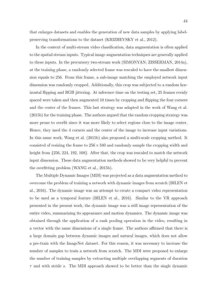
44
that enlarges datasets and enables the generation of new data samples by applying label-
preserving transformations to the dataset (KRIZHEVSKY et al., 2012).
In the context of multi-stream video classification, data augmentation is often applied
to the spatial stream inputs. Typical image augmentation techniques are generally applied
to these inputs. In the precursory two-stream work (SIMONYAN; ZISSERMAN, 2014a),
at the training phase, a randomly selected frame was rescaled to have the smallest dimen-
sion equals to 256. From this frame, a sub-image matching the employed network input
dimension was randomly cropped. Additionally, this crop was subjected to a random hor-
izontal flipping and RGB jittering. At inference time on the testing set, 25 frames evenly
spaced were taken and then augmented 10 times by cropping and flipping the four corners
and the center of the frames. This last strategy was adapted in the work of Wang et al.
(2015b) for the training phase. The authors argued that the random cropping strategy was
more prone to overfit since it was more likely to select regions close to the image center.
Hence, they used the 4 corners and the center of the image to increase input variations.
In this same work, Wang et al. (2015b) also proposed a multi-scale cropping method. It
consisted of resizing the frame to 256× 340 and randomly sample the cropping width and
height from {256, 224, 192, 168}. After that, the crop was rescaled to match the network
input dimension. These data augmentation methods showed to be very helpful to prevent
the overfitting problem (WANG et al., 2015b).
The Multiple Dynamic Images (MDI) was projected as a data augmentation method to
overcome the problem of training a network with dynamic images from scratch (BILEN et
al., 2016). The dynamic image was an attempt to create a compact video representation
to be used as a temporal feature (BILEN et al., 2016). Similar to the VR approach
presented in the present work, the dynamic image was a still image representation of the
entire video, summarizing its appearance and motion dynamics. The dynamic image was
obtained through the application of a rank pooling operation in the video, resulting in
a vector with the same dimensions of a single frame. The authors affirmed that there is
a large domain gap between dynamic images and natural images, which does not allow
a pre-train with the ImageNet dataset. For this reason, it was necessary to increase the
number of samples to train a network from scratch. The MDI were proposed to enlarge
the number of training samples by extracting multiple overlapping segments of duration
τ and with stride s. The MDI approach showed to be better than the single dynamic

45
image approach.
This MDI approach is particularly similar to the data augmentation used in the present
work to extract multiple crops from the SEVR. In this extraction, we experiment different
values for the stride s with a fixed length for the crops. Based on the findings of Wang et
al. (2015b), we choose to use fixed locations for the crops instead of randomly selecting
their positions. These details are discussed in Chapter 5.

46
4 PROPOSED METHOD
The proposed method is divided into two parts, both aiming action recognition in videos.
The first one consists of the presentation of a new approach of VR extraction dubbed
WVR. Additionally, we also defined a specific data augmentation method for the VR
named symmetric extension. Throughout this chapter ways to explore this data augmen-
tation method for the HAR problem are presented. The second part of the proposed
method consists of the usage of both horizontal and vertical WVR, as well as its augmen-
tations, as new spatiotemporal streams. To this end, these streams are used together with
the spatial and temporal streams, respectively RGB frames and OF, in a multi-stream
architecture as illustrated by Figure 4.1. We expect that the VR could be complemen-
tary to the other streams because of its distinct nature that merges temporal and spatial
features. To this end, we propose a new method for extracting the Visual Rhythm (VR)
named Weighted Visual Rhythm (WVR). Two instances of the WVR, depicted in purple
in the Figure 4.1, are employed as spatiotemporal streams.
Figure 4.1: Final multi-stream architecture. The training of each stream is performedindividually, and a weighted sum of the feature maps determines a descriptor utilized inthe final classification.

47
4.1 WEIGHTED VISUAL RHYTHM
The proposals of Concha et al. (2018) and Souza (2018) that take the mean VR formed by
all rows or columns, was adapted. In that proposal, the VR was extracted by taking the
mean color value of the frames across the horizontal or vertical direction. By weighting
the scene elements far from the main object’s or actor’s location as the closest ones, one
might hinder the motion representation. It is expected that the main events recorded in
the video have been framed in its central region. Thus, the underlying moving object or
person in a video is more likely to be observed far from the frame borders. Instead of
the homogeneous weighting, we propose to weight less as the pixels get farther from a
reference row or column. Taking these premises into account and the VR definition of
Chapter 2, we defined the WVR as follows. Let Pr = {(r, 1), (r, 2), · · · , (r, w)} be the set
of points forming the row r. We define the horizontal WVR as:
WVRy =h∑r=1
V RPr · g(r − y, σy) ·
[h∑r=1
g(r − y, σy)
]−1
, (4.1)
where y is the reference row of the horizontal VR and g(s, σ) = e−s2
σ2 is the weighting
function that decays as the other VRs get farther from the reference row y. Conversely,
the vertical WVR can be defined in the same way. Let Pc = {(1, c), (2, c), · · · , (h, c)} be
the set of points forming the column c. We define the vertical WVR as:
WVRx =w∑c=1
V RPc · g(c− x, σx) ·
[w∑c=1
g(c− x, σx)
]−1
, (4.2)
where x is the reference column of the vertical VR and g(s, σ) = e−s2
σ2 is again the
weighting function that in this case decays as the other VRs get farther from the reference
column x. Thus, the WVRs used in the present work are defined by two parameters: the
reference row y and standard deviation σy, for the horizontal version; and the reference
column x and standard deviation σx, for the vertical one. In practice, some simplifications
are adopted. An interval y± dy is defined from σy such that outer rows have zero weight.
Furthermore, to make the parameter y invariant to video height h, we define a factor αy
such that y = αy · h. Those same simplifications also apply for the vertical VRs. An
interval x ± dx is defined from σx such that outer columns have zero weight, and the αy
factor is defined as x = αx · w to make the x parameter invariant to the video width w.

48
Figure 4.2 (a) depicts a video of the biking class from the UCF101 dataset (240 frames
with 320× 240 pixels), forming a horizontal WVR of 320× 240 elements and Figure 4.2
(b) depicts the same video forming a vertical WVR of 240× 240 pixels.
y σ y
(a)
xσx
(b)
Figure 4.2: Weighted Visual Rhythm of a sample video of the class biking from UCF101dataset: y is the middle row in the horizontal rhythm (a), and x is the middle column inthe vertical rhythm (b), and σx and σy are both equal to 33.
Notice that the WVR can be seen as a middle term between the simple VR defined in
Chapter 2 and the VR used by Concha et al. (2018) that takes the mean across all rows
or columns. In the extreme case, when σy or σx assumes large values, the WVR has no
distinction if compared to the mean VR. Figure 4.3 illustrates such comparisons using the
same video from the previous examples. Although the work of Concha et al. (2018) had
extracted the VR from the black and white version of the videos, here we also make the
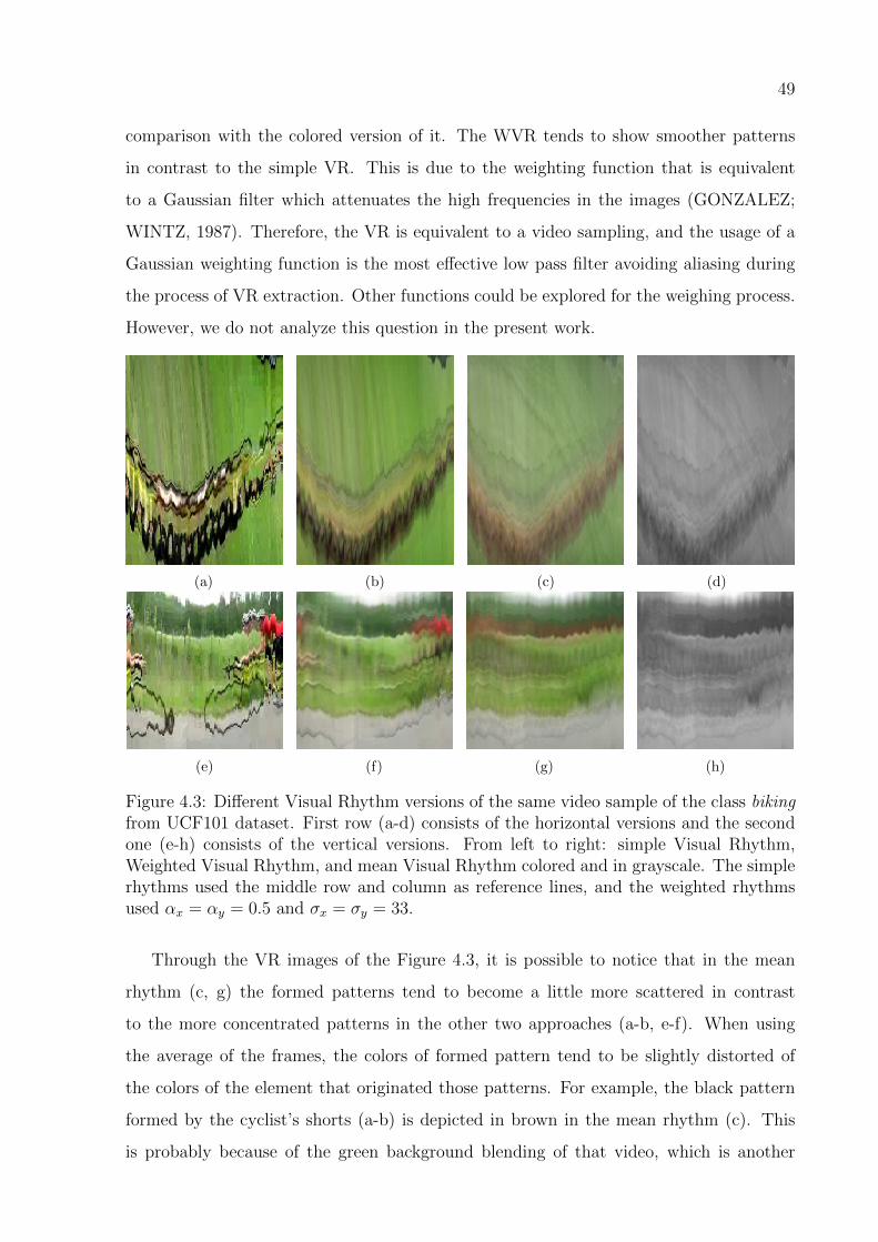
49
comparison with the colored version of it. The WVR tends to show smoother patterns
in contrast to the simple VR. This is due to the weighting function that is equivalent
to a Gaussian filter which attenuates the high frequencies in the images (GONZALEZ;
WINTZ, 1987). Therefore, the VR is equivalent to a video sampling, and the usage of a
Gaussian weighting function is the most effective low pass filter avoiding aliasing during
the process of VR extraction. Other functions could be explored for the weighing process.
However, we do not analyze this question in the present work.
(a) (b) (c) (d)
(e) (f) (g) (h)
Figure 4.3: Different Visual Rhythm versions of the same video sample of the class bikingfrom UCF101 dataset. First row (a-d) consists of the horizontal versions and the secondone (e-h) consists of the vertical versions. From left to right: simple Visual Rhythm,Weighted Visual Rhythm, and mean Visual Rhythm colored and in grayscale. The simplerhythms used the middle row and column as reference lines, and the weighted rhythmsused αx = αy = 0.5 and σx = σy = 33.
Through the VR images of the Figure 4.3, it is possible to notice that in the mean
rhythm (c, g) the formed patterns tend to become a little more scattered in contrast
to the more concentrated patterns in the other two approaches (a-b, e-f). When using
the average of the frames, the colors of formed pattern tend to be slightly distorted of
the colors of the element that originated those patterns. For example, the black pattern
formed by the cyclist’s shorts (a-b) is depicted in brown in the mean rhythm (c). This
is probably because of the green background blending of that video, which is another

50
point to highlight. The green color covering a large area of these generated rhythms is
a strong indication that the action portrayed is performed outdoors. This information
can be useful to restrict classification to actions that are normally performed outdoors.
This type of information is impossible to obtain using grayscale rhythms (d, h). However,
these observations are based on only one video sample and do not assess the superiority of
one approach over another. To investigate the real impact of using one VR over another,
in Chapter 5 we explore the sigma parameters σy and σx. High accuracy with a little
value of sigma would be indicative in favor of the simple VR, and the extreme opposite
would favor the mean rhythm. However, we expect that a median value for sigma achieve
the best results and corroborate to our hypothesis that the central region contains more
relevant information for HAR in videos.
4.2 SYMMETRIC EXTENSION
As stated in Section 3.4, data augmentation is an important method to increase the
number of data samples available to train a DL architecture and, consequently, increase
performance. In CV context, data augmentation consists of applying label-preserving
transformations to original samples presented in a dataset to obtain new samples (FAWZI
et al., 2016).
Since the VR can be interpreted as an image, one could propose to employ standard
techniques of image data augmentation. However, the temporal nature of one of its
dimensions demands some cautions. A rescaling transformation, for instance, would be
equivalent to modify the sample rate of the original video. To illustrate this case, Figure
4.4 shows the effects of up-sampling two VRs, one from the class run (a) and another from
the class walk (b), both from the HMDB51 dataset. In these VRs, inclined thin lines depict
the main pattern of both actions (highlighted in yellow rectangles). An obvious distinction
between these patterns is the inclination angle, which becomes less prominent after the
transformations in both images. This is due to the video sample of the run class has only
a few frames. Thus, resizing dilates the action pattern along the time dimension. This
distortion would not be a problem if the transformation could be applied homogeneously
to all samples. But, since each video has a different duration, this is not possible.
When using VRs, the described situation turns to a problem considering that some
video samples does not have enough frames to reach the required input dimension of
51
320 x 33
up-sampling
run
up-sampling
walk
299 x 299
299 x 299432 x 259
(a) (b)
Figure 4.4: Up-sampling of two different Visual Rhythms from HMDB51 dataset. Theyellow rectangles highlight the main action pattern of each rhythm. Notice that, afterthe transformation, the angles of inclination of each action pattern become closer to eachother in contrast to the obvious distinction between them previously.
the employed network (299 × 299 for InceptionV3). Concha et al. (2018) proposed to
handle this question by repeating the video frames from the beginning until they reach
the necessary amount of frames. However, this approach creates abrupt discontinuities
in the VR that could harm the recognition. Instead of doing this, in the present work,
we propose to repeat the frames backward in time, avoiding sudden cuts, and creating a
symmetric extension for the VR. The symmetric extension of a horizontal WVR is defined
as:
SEVRy(i, k) =
WVRy(i, f −m), for bk/fc odd
WVRy(i,m+ 1), otherwise
(4.3)
where 1 ≤ i ≤ w, m is the remainder of the integer division of k by f and k ∈ Z.
Analogously, the symmetric extension of a vertical WVR is defined as:
SEVRx(i, k) =
WVRx(i, f −m), for bk/fc odd
WVRx(i,m+ 1), otherwise
(4.4)
where 1 ≤ i ≤ h, m is the remainder of the integer division of k by f and k ∈ Z. Thus,
the SEVR is composed of several copies of the VR concatenated several times along the
temporal dimension with the even occurrences being horizontally flipped. Figure 4.5

52
shows both horizontal (a) and vertical (b) WVRs of a video of the biking class of UCF101
extended three times. The premise is as follows: we observed that symmetrical gestures
constitute the majority of actions, e.g. typing, brushing teeth, drumming, pull ups, playing
guitar, etc. Thus, the action performed backward in time also represents the class and can
be used to reinforce the CNN training. The symmetric extension circumvents the temporal
limitation of videos and turns feasible the application of some data augmentation methods.
t
x
f 2f 3f 4f
hCNN
0 s 2s 3s 4s 5s 6s
wCNN
wCNN
wCNN
wCNN
wCNN
(a)
t
Y
f 2f 3f 4f
hCNN
0 s 2s 3s 4s 5s 6s
wCNN
wCNN
wCNN
wCNN
wCNN
(b)
Figure 4.5: Extraction of five squared crops from the symmetric extensions of both hor-izontal (a) and vertical (b) Visual Rhythms of the same video of the class biking fromUCF101 dataset. The frame width is w = 320 pixels, the frame height is h = 240 pixels,and the corresponding video length is f = 240 frames. The stride between crops is s = 150pixels and the crop dimensions are wCNN = hCNN = 299. The central area in X is selectedin (a) and in (b) the rhythm will be stretched in Y to cover the crop dimensions.

53
4.2.1 Symmetric Extension with Fixed Stride Crops
With the SEVRs, it is possible to obtain crops to match the required input dimension
of the employed network. We propose to go further and extract more than one crop per
video and, consequently, augmenting the available data. The observation that supports
this idea is that long duration video samples usually exhibit the action more than once.
The symmetric extension allows short video samples to share this same behavior. Hence,
a crop would possibly contain a full cycle of the action, even being only a fraction of the
entire VR or the SEVR.
We propose to use multiple crops from each extended VR as a data augmentation
process. Each crop is formed by the image constrained in a window of dimensions wCNN×
hCNN (matching the CNN’s input). A crop Cxt from the horizontal SEVR with lower left
coordinates x and t is defined as:
Cxt(a, b) = SEVRy(x+ a, t+ b), (4.5)
with x ≤ a < x + hCNN and t ≤ b < t + wCNN. And a crop Cyt from the vertical SEVR
with lower left coordinates y and t is defined as:
Cyt(a, b) = SEVRx(y + a, t+ b), (4.6)
with y ≤ a < y+hCNN and t ≤ b < t+wCNN. The VR is extended symmetrically until nc
crops are extracted using a stride s, i.e., the first crop is taken at t = 0 and all subsequent
nc − 1 crops are taken s frames ahead the previous one. The resulting set of crops for a
fixed row x is {Cxt | t = js}, for j ∈ {0, 1, ..., nc − 1}, and similarly, the resulting set of
crops for a fixed column y is {Cyt | t = js}, for j ∈ {0, 1, ..., nc − 1}.
If hCNN is smaller than the spatial dimension of the SEVR, i.e., the video frame width
or height is greater than the corresponding dimension of the CNN, the crops are centered
in the spatial dimension. Figure 4.5 (a) depicts this case for the SEVRy. This approach
assumes that the main action motion is mostly performed in these central regions. Notice
that the crops do not reach the top and bottom sides. To include these regions, extra nc
crops keeping the stride s from each other are obtained, aligned with the top and bottom
borders. Thus, up to 3 · nc crops can be obtained depending on the application. This is
useful to get all information in X and for most videos reinforce the central information.

54
Now, if hCNN is bigger than the spatial dimension of the SEVR, i.e., the video frame width
or height is smaller than the corresponding dimension of the CNN, the crops are stretched
in the spatial dimension to satisfy the network’s input size. Figure 4.5 (b) depicts this
case for the SEVRx. The stride used in Figure 4.5 is only used for illustration purposes.
There is no guarantee that a complete cycle of the action is portrayed in a single crop
since we do not have any information about its commencement and conclusion in a video
sample. This is another reason to use multiple crops. The probability of getting at least
one complete cycle of action increases proportionally with the number of excerpted crops.
Besides that, the stride could be helpful for this purpose. This parameter is an attempt
to adjust the temporal limits of the crop, aiming to comprehend a full action cycle. To
this end, in Chapter 5, we empirically explore distinct values for the stride s together with
multiple crops.
4.3 SPATIOTEMPORAL STREAM CLASSIFICATION PROTOCOL
An overview of the proposed method for a spatiotemporal stream using WVRs is depicted
in Figure 4.6. It consists of a testing classification protocol using a version of the Incep-
tionV3 network (SZEGEDY et al., 2016) with WVRs. This overview applies to both
horizontal and vertical rhythms, but they are explored separately. Thus, two NNs are
trained independently.
A WVR is computed for each video, and its data augmentation is driven by symmetric
extension. Multiple crops with fixed stride are extracted from the symmetric extension.
At the inference time and for video classification, all the augmented crops are individually
applied to the CNN, and their last layer feature maps are extracted (just before softmax
classification) and averaged. We observed that fusing the feature maps before the softmax
normalization, as performed by Diba et al. (2017) and Zhu et al. (2018), achieves better
results. A softmax classification layer is applied to this average feature map. The softmax
is a function that takes as input a vector of real numbers of dimension N and normalizes
it into a probability distribution consisting of N probabilities. The ideal classifier would
have 1 in the index correspondent to the correct class and zero in the other positions. The
final class prediction is the averaged prediction of all crops.
We argue that this process might yield better class predictions based on the assumption
that multiple crops taken at different time positions are representative of a distinct portion

55
Figure 4.6: Overview of the proposed Visual Rhythm stream. After the symmetric ex-tension, nc crops apart from each other by a stride s are extracted in the center (yellow).Depending on the dataset, extra crops aligned with the image top (magenta) and bot-tom (cyan) are extracted. All crops are applied to the CNN. The resulting features areaveraged, and the final class is predicted through a softmax layer.
of the underlying action in the video. In the training stage, however, each crop is processed
as a distinct sample and separately classified, i.e., the average is not taken into account.
The WVR parameters, as well as the SEVR parameters, are explored in Chapter 5 using
the described spatiotemporal stream and classification protocol.

56
4.4 MULTI-STREAM CLASSIFICATION PROTOCOL
Two instances of the spatiotemporal stream, one operating on horizontal WVRs and an-
other operating on vertical WVRs, are used together with the already discussed spatial
and temporal streams to form a multi-stream architecture. In the overview of the pro-
posed multi-stream architecture, depicted in Figure 4.1, the spatiotemporal streams are
represented in purple, and the spatial and temporal streams, already explained in Sections
2.4 and 2.5, are represented in orange and blue, respectively.
Each stream is trained individually, and all of them use a version of the InceptionV3
network pre-trained with ImageNet. The following details concern to both UCF101 and
HMDB51 datasets. We adopt the improved spatial stream described by Concha et al.
(2018) as well as the training and testing protocols used in that work. More specifically,
in this stream, two random frames per video, one from each half of the video, are used
as a representation of each sample in the training phase. In the testing phase, 25 frames
are taken uniformly over the video length. The CNN receives one frame at a time in both
phases. We use the multi-crop augmentation with horizontal flips proposed by Wang et
al. (2015b). Thus the test prediction is performed by averaging 250 feature maps.
For the temporal stream, a stack of 10 consecutive OFs, extracted from a random
initial position in the video, fed the network. Hence, the input has 20 channels since the
OF is decomposed into horizontal and vertical components. The stack size is based on
the results of Simonyan and Zisserman (2014a) and Wang et al. (2015b).
The testing phase of the temporal stream is very similar to the spatial stream: a
stack of 25 evenly sampled OFs and its augmentations obtained through multi-crop and
horizontal flip transformations are employed together to classify the video. The spatiotem-
poral streams in this multi-stream architecture follow the training and testing protocols
described in the previous section.
A fusion of the feature maps of each stream produces the final classification for the
multi-stream architecture. This fusion is a weighted sum of the feature maps. A grid
search strategy is used to find out the best weights.
The feature maps used for this are also extracted before the application of the softmax.
Section 5.2 gives implementation details about both spatiotemporal stream and multi-
stream architectures.

57
5 EXPERIMENTAL RESULTS
In this chapter, we evaluate the proposed methods: WVR and SEVR, and the multi-
stream architecture using SEVRs. The spatiotemporal stream is assessed by exploring
different values for some parameters. It is possible to note that, with a particular set
of parameters, a significant performance increase can be achieved for the WVR stream
if compared to the baseline. Furthermore, to make our results more competitive and to
show the complementarity of the spatiotemporal streams, we explore the multi-stream
classification using every possible combination between the employed streams: horizontal
WVR, vertical WVR, static RGB frames, and OF.
5.1 DATASETS
The proposed method was evaluated through experiments performed on two challenging
video action datasets: UCF101 (SOOMRO et al., 2012) and HMDB51 (KUEHNE et al.,
2013).
The UCF101 dataset contains 13320 videos. All videos have a fixed frame rate and
resolution of 25 FPS and 320×240 pixels, respectively. This dataset covers a broad scope
of actions from the simplest to the most complex ones. An example of the latter is playing
some sport or playing some instrument. These videos were collected from YouTube and
divided into 101 classes. Since multiple users uploaded them, there is a great diversity
in terms of variations in camera motion, object appearance and pose, object scale, and
viewpoint. This diversity is essential to replicate the variety of actions that a realistic
scenario can have.
HMDB51 is an action recognition dataset containing 6766 videos with 51 different
action classes. The HMDB51 includes a wide variety of samples collected from various
sources, including blurred videos, or with low quality, and actions performed in distinct
viewpoints. Most videos of this dataset originate from movies and a small fraction from
public databases, such as the Prelinger archive, YouTube, and Google videos. There is no
fixed resolution for the HMDB51 videos.
The evaluation protocol used for both datasets is the same. The average accuracy of
the three training/testing splits available for both datasets is reported as the final result.

58
5.2 IMPLEMENTATION DETAILS
All the code was implemented with Python programming language. For the spatial and
temporal stream parts of the multi-stream architecture, we used the implementation of the
“Multi-Stream Convolutional Neural Networks for Action Recognition in Video Sequences
Based on Adaptive Visual Rhythms” (CONCHA et al., 2018) available on GitHub1. In
the present work, as well as in Wang et al. (2015b), the authors utilized the TVL1 method
(ZACH et al., 2007) for the OF extraction. More specifically, the implementation present
in the OpenCV library.
The WVR computation is carried out in two steps, which are applied to each video
frame. The application of a 1D Gaussian filter, implemented in the SciPy Python module2,
and the extraction of the reference row or column from the frame. Remember that the
rows outside the interval y± dy have zero weight what implies that the total width of the
employed filter will be 2 · dy. The filter width defines the area within which elements will
influence the calculation of the WVR. We empirically fixed the dy value (equivalent to the
truncate parameter in the SciPy implementation) to be 1.5 · σy. Thus, the filter spans a
total width of 3·σy and covers approximately 87% of the values of the normal distribution.
This also applies to the vertical rhythm and the dx, σx and x parameters. Since we are
interested in verifying which portion of the frame most motion are performed, this fixed
value fits our purposes. The Gaussian filter was applied only across the corresponding
axis of rhythm direction in question, i.e., the filter was applied to the Y axis of the frame
when extracting the horizontal rhythm and to the X axis when extracting the vertical
rhythm. The OF and WVR extractions were performed as pre-processing steps.
The Keras framework (CHOLLET et al., 2015) was used for all experiments con-
cerning to the spatiotemporal streams. A slightly modified version of the InceptionV3
network (SZEGEDY et al., 2016) initialized with ImageNet (DENG et al., 2009) weights
was used in the experiments of Sections 5.3 and 5.4. The InceptionV3 was modified to
have an additional fully connected layer with 1024 neurons and 60% of dropout. The
softmax classifier was adapted to match the number of classes in each dataset.
All training parameters were kept the same for both datasets. Some Keras random
data augmentation approaches (horizontal flip, vertical flip, and zoom in the range of
1https://github.com/darwinTC/Adaptive-Visual-Rhythms-for-Action-Recognition2https://docs.scipy.org/doc/scipy-0.15.1/reference/generated/scipy.ndimage.filters.gaussian fil-
ter1d.html

59
0.8 to 1.2) were applied to the input images. These augmentations were performed in
runtime by the framework while the fixed stride crop augmentation, described in Section
4.2, was performed previously as a pre-processing step. We show in Section 5.5 that
these data augmentations drive to a significant accuracy increase.The mean RGB values
were centered in zero and normalized. To this end, the Wedford’s methods of mean and
standard deviation accumulative computation (WELFORD, 1962) were incorporated into
the Keras framework. This method was used to take advantage of the framework ability to
work with batches of data and save memory. The network was trained with the following
parameters: learning rate of 1e−3, batch size of 16, Stochastic Gradient Descent (SGD)
optimizer with momentum of 0.9 and categorical cross entropy loss function. The early
stop training strategy was adopted with patience of 6 epochs. The learning rate was also
scaled down by a factor of 10 after 3 epochs without any improvement in the loss function.
The learning rate minimum value was limited to 1e−6.
Various machines were used in the experiments. The implementation of the WVR
extraction was CPU-bound while all DL architectures took advantage of GPU processing.
The machine used for the WVR extraction has an Intel® Xeon® E5-4607 processor with
48 threads and 32GB of RAM. Our code was designed to work in a parallel manner and
extract the VR of one video per thread available in the machine. Among the machines
used for DL architecture training, the following graphic cards were used individually:
NVIDIA® Titan Xp, NVIDIA GeForce® RTX 2080 Ti, NVIDIA Titan V, and NVIDIA
GeForce GTX 1080.
The baseline method to assess the improvement achieved with the proposed method
comprehend the usage of the WVR without the symmetric extension and, consequently,
without the fixed stride crops. The WVR is resized to match the network input dimen-
sions. All the network details described in the previous paragraph were also used in this
baseline method. Table 5.1 shows the accuracy achieved by the baseline method with
horizontal and vertical rhythms, WVRy and WVRx respectively.
Table 5.1: Baseline accuracy rates (%) for UCF101 and HMDB51.
Method UCF101 (%) HMDB51 (%)
WVRy 65.19 34.46
WVRx 60.41 32.37

60
The representation of the video through the WVR depends on the choice of two param-
eters: a reference row αy or column αx and the standard deviation σy or σx. The impacts
of these parameters are explored in the first two experiments. The results show that
the right choice of these parameters can help to improve the accuracy in both datasets.
These results also provide evidence that the main action of the videos tends to focus on
a particular region of the frames. We also perform experiments varying the symmetrical
extension parameters aiming to achieve better settings for it. The results corroborate
the assumption that a data augmentation method is essential for increasing the accuracy
rates. The following sections discuss the experiments of the horizontal WVR and the
vertical WVR separately, in this same order.
5.3 HORIZONTAL VISUAL RHYTHM PARAMETERIZATION
A sequence of experiments was performed to discover the best set of parameters for the
SEVRy. The baseline mean accuracy in this case is 65.19% and 34.46% in UCF101 and
HMDB51 datasets (Table 5.1), respectively, and the baseline parameters were: αy =
0.5 and σy = 33. Throughout the experiments, the best parameters are employed in
the subsequent executions. Initially, the parameters used for WVR and the symmetric
extension are: αy = 0.5 (middle row), nc = 1 and only the central crop in X is extracted.
Since InceptionV3 expects input images of 299× 299 pixels, wCNN and hCNN are both set
to 299. The method depicted in Figure 4.2 was employed in all experiments.
In the first experiment, we compare the impact of the variation of the σy parameter.
The following values for σy were tested: 7, 15, 33, 49 and 65. These values were chosen to
verify if the region within the action occurs is concentrated in a small area or it is more
vertically spread. According to the truncation of applied the Gaussian filter, the value
33 spans approximately 1/3 of the frame width. We empirically chose this value as the
starting point for selecting the other valuers. The values smaller than 33 are approximately
half and the 1/4 of the starting point, and the bigger ones are approximately the 50%
increase and the double. The results are shown in Table 5.2. The better standard deviation
for UCF101 was 33, and for HMDB51 it was 15. This indicates that actions on UFC101
tend to occur in a more spread region compared to HMDB51 since a smaller standard
deviation means more concentrated Gaussian weighting around the middle row.
In the second experiment, we show the influence of the reference row on the accuracy

61
Table 5.2: Comparison of accuracy rates (%) for UCF101 and HDMB51 varying the σyparameter.
σy UCF101 (%) HMDB51 (%)
7 63.29 33.66
15 63.85 33.99
33 65.26 33.40
49 64.62 32.24
65 63.00 31.46
rate. As mentioned earlier, a factor αy is used instead of the parameter y. We explore
values close to the center of the video, expecting that the scene tends to be framed in
the center of the video. The values chosen for the factor were: 0.40, 0.45, 0.50, 0.55
and 0.60. Values above 0.5 indicate the lower part of the image. Because the samples in
both datasets come from multiple sources, the main action in each video may not happen
exactly in the center of the video. This is the case of the UCF101. It was empirically
observed that the better results were obtained when the reference row is located just below
the center of the video. The mean action position in this dataset tends to be horizontally
shifted around 5% below the center of the video (Table 5.3).
Table 5.3: Comparison of mean accuracy rates (%) of UCF101 and HMDB51 varying theαy factor.
αy UCF101 (%) HMDB51 (%)
0.40 62.82 30.06
0.45 64.83 31.00
0.50 65.26 33.99
0.55 65.32 33.35
0.60 65.24 33.48
In the next experiment, the number of crops nc is increased to check if the accuracy
rate also increases. The premise is that with more crops, it is possible to cover the entire
temporal extension of the video present in SEVR. It is expected that the new crops
incorporate more discriminant aspects of the video. As mentioned before, the additional
crops also increase the probability to get at least one crop matching an entire cycle of
action. The nc values used are: 1, 2, 3 and 4. In this experiment, the stride s between
the crops is fixed to 299 matching the wCNN size. Thus, consecutive and non-overlapping
crops are obtained. Table 5.4 shows the results of this experiment. The results endorse

62
the expected correlation between nc and the accuracy rate. We could explore even bigger
values for nc. However, we chose not to perform experiments with larger values because
of the time spent in the training, that was almost 2 days for all splits of UCF101 and
HMDB51, using the Titan Xp graphics card and nc = 4. For the next experiments, we
set the number of crops to 4.
Table 5.4: Comparison of accuracy rates (%) of UCF101 and HMDB51 datasets varyingnc parameter.
nc UCF101 (%) HMDB51 (%)
1 65.32 33.99
2 65.64 34.42
3 66.19 34.03
4 67.70 34.99
The fourth experiment consists of using crops that overlap each other along the time
dimension. When the extended WVR completes a cycle, it begins to repeat its temporal
patterns, as shown in Figure 4.5. In the even WVR copies, those patterns are horizontally
flipped. Crops can be extracted along the extended time dimension with or without direct
overlapping, consecutively or not. Consecutive and non-overlapping neighbor crops are
obtained with s = wCNN, as in the previous experiment. Gaps between the crops are
obtained by using stride s > wCNN. Overlaps between consecutive crops occur when using
s < wCNN. In the present work, we investigate the cases having 0 < s ≤ wCNN. Notice
that multiple parts of the WVR, forward or backward in time, will be repeated if
wCNN + (nc − 1) · s > f (5.1)
is satisfied. Previous to the training, the rhythm is extended according to the number of
crops nc and the stride s employed in the experiment. Hence, the video samples satisfying
Equation 5.1 are extended. Among the UCF101 videos, this occurs to 93.75% using stride
13, 95.47% using stride 25, and to all videos except for one using strides 274, 286, and
299. Concerning the HMDB51 videos, this occurs to 98.32% using stride 13, 98.82% using
stride 25, and occurs all videos using the other values of stride. Table 5.5 display this
statistic.
We used the strides 13, 25, 274, 286 and 299. According to the frame rate, these values
have a direct relation with the time in video . Since all videos have 25 fps, each 25 columns
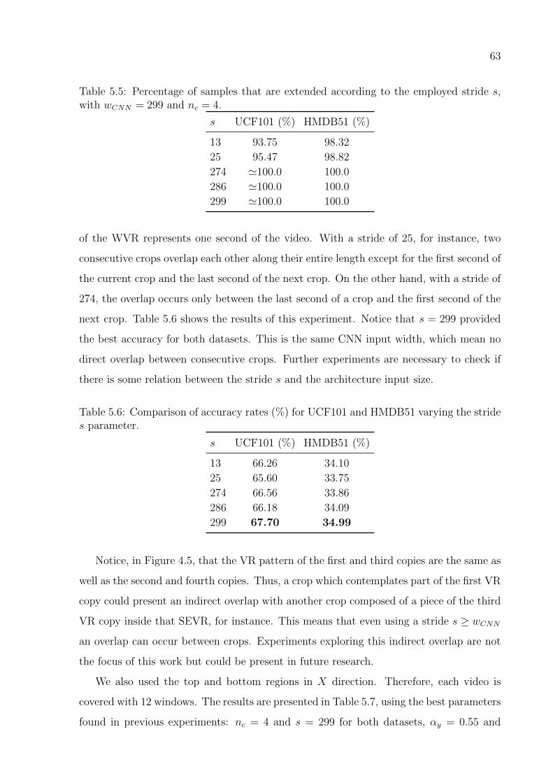
63
Table 5.5: Percentage of samples that are extended according to the employed stride s,with wCNN = 299 and nc = 4.
s UCF101 (%) HMDB51 (%)
13 93.75 98.32
25 95.47 98.82
274 '100.0 100.0
286 '100.0 100.0
299 '100.0 100.0
of the WVR represents one second of the video. With a stride of 25, for instance, two
consecutive crops overlap each other along their entire length except for the first second of
the current crop and the last second of the next crop. On the other hand, with a stride of
274, the overlap occurs only between the last second of a crop and the first second of the
next crop. Table 5.6 shows the results of this experiment. Notice that s = 299 provided
the best accuracy for both datasets. This is the same CNN input width, which mean no
direct overlap between consecutive crops. Further experiments are necessary to check if
there is some relation between the stride s and the architecture input size.
Table 5.6: Comparison of accuracy rates (%) for UCF101 and HMDB51 varying the strides parameter.
s UCF101 (%) HMDB51 (%)
13 66.26 34.10
25 65.60 33.75
274 66.56 33.86
286 66.18 34.09
299 67.70 34.99
Notice, in Figure 4.5, that the VR pattern of the first and third copies are the same as
well as the second and fourth copies. Thus, a crop which contemplates part of the first VR
copy could present an indirect overlap with another crop composed of a piece of the third
VR copy inside that SEVR, for instance. This means that even using a stride s ≥ wCNN
an overlap can occur between crops. Experiments exploring this indirect overlap are not
the focus of this work but could be present in future research.
We also used the top and bottom regions in X direction. Therefore, each video is
covered with 12 windows. The results are presented in Table 5.7, using the best parameters
found in previous experiments: nc = 4 and s = 299 for both datasets, αy = 0.55 and

64
σy = 0.33 for UCF101 and αy = 0.5 and σy = 0.15 for HMDB51. Its worth note that some
videos from HMDB51 (around 6.03%) did not benefit from the extra crops or benefited
very poorly due to their frame width being under of wCNN or very close to it. Thus,
the new crops did not add supplementary information about the video aspects. Still, the
extra eight crops helped to increase the accuracy rate in both datasets. Similar to the
previous experiment, the use of the other regions produced an overlap between the crops
along the spatial dimension. However, more experiments need to be performed to assess
how the overlap in X can be explored for data augmentation.
Table 5.7: Comparison of accuracy rates (%) for UCF101 and HMDB51 when extra cropsare used.
Regions UCF101 (%) HMDB51 (%)
Central 67.70 34.99
Central + Top + Bottom 68.01 35.29
Figure 5.1 show for UFC101 and HMDB51 the mean accuracy difference between the
best result of SEVRy (Table 5.7) and the baseline method WVR. Blue bars mean the
SEVRy were better by the given amount. Conversely, red bars favor the WVR. For the
UCF101, SEVRy performs better in 68 classes, worse in 32 classes, with even results in 1
classes. For the HMDB51, SEVRy performs better in 25 classes, worse in 23 classes, with
even results in 3 classes. The classes which demonstrated improvement for the proposed
method seem to share some characteristics among each other. They often present actions
with certain cyclic movements (e.g., brushing teeth, playing violin, typing). This kind of
action takes full advantage of the SEVRy. Since the reverse movement generates patterns
very similar to the one generated by the original movement, the multiple crops reinforce
this kind of action and increase the accuracy of them, corroborating with our premise.
In UCF101, the top-5 actions where SEVR was inferior to WVR are apply lipstick,
drumming, handstand push ups, pull up and push up, respectively indices 2, 27, 37, 70
and 72, and the top-5 actions where SEVR was superior to WVR are biking, cutting
in kitchen, mopping floor, playing dhol and tai chi, respectively indices 11, 25, 55, 61
and 91. In HMDB51, the top 5 actions where SEVR was inferior to WVR are dive,
punch, ride horse, shoot gun and sit up, respectively indices 8, 28, 32, 37 and 39, and
the top 5 actions where SEVR was superior to WVR are catch, drink, eat, handstand
and laugh, respectively indices 3, 11, 12, 17 and 24. On both datasets, some of the top-

65
1 11 21 31 41 51 61 71 81 91 101Classes
0.0
0.1
0.2
0.3
0.4
Accu
racy
SEVRy
WVRy
(a) UCF101
1 11 21 31 41 51Classes
0.0
0.1
0.2
Accu
racy
SEVRy
WVRy
(b) HMDB51
Figure 5.1: Mean accuracy difference for each class between SEVRy and WVRy forUCF101 (a) and HMDB51 (b). Blue bars indicate that SEVR performs better by thegiven amount while red bars favor WVR.
5 actions that performed worst with SEVR in comparison with WVR are actions that
could be treated as cyclic actions and thus exploited better the symmetric extension (e.g.
puch, pull up and push up). Analogously, some actions that apparently do not show
cyclic motion patterns and possibly be harmed by the symmetric extension are present
in the top-5 actions where SEVR performed better than WVR (e.g. tai chi, catch and
handstand). Despite that, the expected behavior of performance enhancement in cyclic
actions can be observed from many of the top-5 actions where SEVR performed better
than WVR, such as biking, cutting in kitchen, mopping floor, playing dhol, drink and
eat. The aforementioned actions apparently do not have common aspects that indicate
when the symmetric extension should be applied. Nevertheless, further investigation is
necessary to understand the effects of employing the symmetric extension in some classes

66
and how this affect the signature patterns generated in the Visual Rhythms.
5.4 VERTICAL VISUAL RHYTHM PARAMETERIZATION
We repeated the same sequence of experiments to discover the best set of parameters for
the SEVRx. The baseline mean accuracy in this case is 60.41% and 32.37% in UCF101 and
HMDB51 datasets (Table 5.1), respectively, and the baseline parameters were: αx = 0.5
and σx = 33. As in the previous section, the best parameter found in one experiment
is also employed in the subsequent experiments. Initially, the parameters used for WVR
and the symmetric extension are: αx = 0.5 (middle column), nc = 1 and only the central
crop in Y is extracted. Since InceptionV3 expects input images of 299× 299 pixels, wCNN
and hCNN are both set to 299. Considering that the videos of the UCF101 dataset have
fixed dimensions of 320× 240, the crops extracted from the vertical WVR are resized in
spatial dimension to match the hCNN dimension. The method depicted in Figure 4.2 was
employed in all experiments.
The first experiment compares the impact of the variation of the σx parameter. The
same values from the horizontal rhythm are used for σx: 7, 15, 33, 49 and 65. The
results are shown in Table 5.8. The better standard deviation for UCF101 was again
33, and for HMDB51 was 65. It is worth noting that the standard deviation 33 for the
vertical rhythm of the UCF101 indicates a more significant scattering if compared with
its horizontal counterpart due to the mentioned size difference between frame dimensions.
The result for HMDB51 indicates an even more spread motion pattern across the vertical
axis in contrast to the value found in the same experiment for the horizontal rhythm of
this dataset.
Table 5.8: Comparison of accuracy rates (%) for UCF101 and HDMB51 varying the σxparameter.
σx UCF101 (%) HMDB51 (%)
7 60.48 27.64
15 61.15 28.50
33 62.22 29.89
49 62.05 30.33
65 60.73 31.39
In the second experiment, we show the influence of the reference column on the ac-

67
curacy rate. As mentioned earlier, a factor αx is used instead of the parameter x. The
values from the corresponding experiment of the previous section repeat here: 0.40, 0.45,
0.50, 0.55 and 0.60. The results of Table 5.9 suggest that the middle column and its
surrounding region are the areas with more occurrence of vertical motion. The best value
for the αx on both datasets was 0.50.
Table 5.9: Comparison of mean accuracy rates (%) of UCF101 and HMDB51 varying theαx factor.
αx UCF101 (%) HMDB51 (%)
0.40 58.14 31.31
0.45 61.06 31.09
0.50 62.20 31.39
0.55 61.47 30.83
0.60 58.42 29.10
In the next experiment, we check if the correlation between the number of windows nc
and accuracy rate holds for the vertical WVR. The premise is the same as the horizontal
rhythm. It is expected that the new crops incorporate more discriminant aspects of the
video and increase the chance of at least one of them contains an entire cycle of action.
The nc values used are: 1, 2, 3 and 4. The stride s between the windows is fixed to
299 matching the wCNN size. Thus, consecutive and non-overlapping crops are obtained.
Table 5.10 show the results of this experiment. Despite some decrease with 3 crops in the
UCF101 and 2 crops in the HMDB51, in the long term, the correlation between nc and
the accuracy rate is showed.
Table 5.10: Comparison of accuracy rates (%) of UCF101 and HMDB51 datasets varyingnc parameter.
nc UCF101 (%) HMDB51 (%)
1 62.20 31.39
2 62.59 29.8
3 61.75 31.72
4 63.50 32.11
The fourth experiment evaluates the stride value s. The same statements about the
stride variation mentioned in the corresponding experiment of the previous section also
concern to the vertical rhythm. The same stride were used: 13, 25, 274, 286 and 299.
68
Table 5.11 shows the results of this experiment. The same results of the horizontal rhythm
have repeated for the vertical one.
Table 5.11: Comparison of accuracy rates (%) for UCF101 and HMDB51 varying thestride s parameter.
s UCF101 (%) HMDB51 (%)
13 62.09 30.22
25 61.90 31.81
274 62.31 30.68
286 62.73 30.15
299 63.50 32.11
The final experiment consisted in the usage of top and bottom regions in Y direction.
However, since the height h of the videos of the UCF101 dataset is smaller than the
hCNN , there is not a reminiscent region to be covered. All the spatial dimension data
is represented in the vertical WVR. Despite this, for completeness of the experiments
and to evaluate the impact of the replication of the exact information contained in one
crop, we have used the same nc crops three times, one for each region (center, top, and
bottom). Therefore, in this experiment, each video was covered by 12 windows using
the best parameters found in the previous experiments for each dataset. The results are
presented in Table 5.12. The impact of the replication is negative for the two datasets.
Consequently, the usage of 4 distinct crops from the vertical rhythm is better than 12
crops with repeated information.
Table 5.12: Comparison of accuracy rates (%) for UCF101 and HMDB51 when extracrops are used.
Regions UCF101 (%) HMDB51 (%)
Central 63.50 32.11
Central + Top + Bottom 62.81 30.85
Figure 5.2 shows for UFC101 and HMDB51 the mean accuracy difference between the
best result of SEVRx (Table 5.12) and the baseline method WVR. Blue bars mean the
SEVRx were better by the given amount. Conversely, red bars favor the WVR. For the
UCF101, SEVRx performs better in 55 classes, worse in 45 classes, with even results in 1
classes. For the HMDB51, SEVRx performs better in 23 classes, worse in 26 classes, with
even results in 2 classes.

69
1 11 21 31 41 51 61 71 81 91 101Classes
0.0
0.1
0.2
0.3
0.4
0.5
0.6
0.7
Accu
racy
SEVRx
WVRx
(a) UCF101
1 11 21 31 41 51Classes
0.0
0.1
0.2
Accu
racy
SEVRx
WVRx
(b) HMDB51
Figure 5.2: Mean accuracy difference for each class between SEVRx and WVRx forUCF101 (a) and HMDB51 (b). Blue bars indicate that SEVR performs better by thegiven amount while red bars favor WVR.
In UCF101, the top 5 actions where SEVR was inferior to WVR are drumming, ham-
mer throw, jumping jack, jump rope and shot put, respectively indices 27, 36, 47, 48 and
79, and the top 5 actions where SEVR was superior to WVR are band marching, cutting
in kitchen, hammering, head massage and playing tabla, respectively indices 6, 25, 35,
39 and 66. In HMDB51, the top 5 actions where SEVR was inferior to WVR are jump,
run, sit, somersault and turn, respectively indices 20, 33, 38, 42 and 49, and the top 5
actions where SEVR was superior to WVR are catch, kiss, laugh, shoot ball and shoot
bow, respectively indices 3, 23, 24, 35 and 36. As noted for the horizontal rhythm, the
results mix some expected and unexpected behaviors. It is worth mentioning that some
classes that were among the top-5 enhanced classes with SEVRy also belong to the same
group concerning to SEVRx: cutting in kitchen from UCF101, and catch and laugh from

70
HMDB51. This reinforces the importance of SEVR to increase these classes accuracies.
5.5 DATA AUGMENTATION ABLATION STUDY
In this section, we present an experiment to evaluate the real contribution of our data
augmentation method apart from Keras data augmentation methods. To this end, we
executed the baseline method without Keras data augmentation (horizontal flip, vertical
flip, and zoom in the range of 0.8 to 1.2). The baseline method does not count with our
proposed data augmentation with fixed stride crops taken from the symmetric extension.
Therefore, this is the scenario without any other data augmentation methods. We already
have the results of the previous sections that take advantage of both data augmentation
methods (Keras and ours). To complete the experiment setup, we already run the scenario
with our data augmentation and without Keras’ data augmentation. Table 5.13 show the
results of these experiments. All results were obtained using the horizontal version of the
WVR. The SEVR scenarios used 4 crops with fixed stride of 299.
Table 5.13: Comparison of accuracy rates (%) for UCF101 and HMDB51 with (w/) andwithout (w/o) data augmentation methods.
ScenariosUCF101 (%) HMDB51 (%)
w/ Keras DA w/o Keras DA w/ Keras DA w/o Keras DA
Baseline 65.19 57.64 34.46 28.93
SEVR 67.70 60.55 34.99 28.80
In both datasets, we can notice that the conventional data augmentation methods
performed for image classification are also applicable for VRs. The results are very signif-
icant with a mean difference of 7.35% and 5.86%, in UCF101 and HMDB51 respectively,
in favor of the usage of Keras data augmentation. The performance increase with our data
augmentation methods on UCF101 was very relevant too. In this dataset, the mean in-
crease was 2.71%. However, for HMDB51, our approach showed a slight decrease without
using Keras data augmentation, 0.13%, and a small increase using both data augmen-
tation methods, 0.53%. In future works, we intend to investigate better the behavior of
data augmentation methods on HMDB51. Overall, the usage of both data augmentation
methods for both datasets leads to the performance increase, highlighting the performance
in UCF101, which increased over 10%.

71
5.6 MULTI-STREAM CLASSIFICATION USING VISUAL RHYTHMS
The goal in this section is to show that our spatiotemporal streams can complement a
multi-stream architecture to get more competitive accuracy rates. The results of indi-
vidual streams are shown in Table 5.14. The first five approaches, Optical Flow, RGB*,
Horizontal-mean, Vertical-mean, and Adaptive Visual Rhythm (AVR), are results from
the work of Concha et al. (2018). It is worth remembering that the use of OF as a
temporal stream is not a contribution of Concha et al. (2018), but of Simonyan and Zis-
serman (2014a). However, the result of such work is shown since it comes from the use
of the InceptionV3 network in the temporal stream, which is not performed in the origi-
nal two-stream work (SIMONYAN; ZISSERMAN, 2014a). Similar to other multi-stream
networks (SIMONYAN; ZISSERMAN, 2014a; WANG et al., 2015b), the OF performs
better in both datasets. It is possible to notice that the horizontal SEVR presented su-
perior performance if compared with the vertical one, independent of the dataset. The
same outcome appeared in the mean rhythm results. Excepting for the SEVRy in the
HMDB51, the SEVR was superior to the mean rhythm approach. Concerning the com-
parison between the SEVRy with the AVR, the results are divided. Even using only
horizontal motion information, the SEVRy is better than AVR in the UCF101 scenario.
However, the lack of vertical information may be one of the factors that led to a worse
result in the HMDB51 dataset.
Table 5.14: Results of single-stream approaches.
Single streams UCF101 (%) HMDB51 (%)
Optical Flow (CONCHA et al., 2018) 86.95 59.91
RGB* images (CONCHA et al., 2018) 86.61 51.77
Horizontal - mean (CONCHA et al., 2018) 62.37 35.57
Vertical - mean (CONCHA et al., 2018) 53.87 30.12
AVR (CONCHA et al., 2018) 64.74 39.63
WVRy 65.19 34.46
WVRx 60.41 32.37
SEVRy 68.01 35.29
SEVRx 63.50 32.11
In order to our approach achieve more competitive results, we proposed a final multi-
stream architecture merging the SEVRy and SEVRx best setups, with the RGB* and the
OF streams. This final combination is not enough to assess the complementarity of the

72
streams. To this end, we also conducted experiments incrementally fusing the streams.
The strategy used for merging the streams was the same described by Concha et al.
(2018). More specifically, to fuse the predictions of all streams, weights were evaluated
through a grid search strategy. For each weight, we tested every value from 0 to 10 with a
0.5 step. We are aware that this is not the best strategy for merging the streams. However,
its adoption allows an impartial attribution of weights and proper comparison between
the results of Concha et al. (2018) with the results of the present work. Besides, the
proposition of a new approach for late fusion is not the focus of the present work. This is
an open question that could be the focus of future works. Concerning the combination of
all streams, the best combination found for UCF101 was 9.0, 7.0, 1.5 and 1.5, respectively
for OF, RGB*, SEVRy and SEVRx. And the best combination found for HMDB51 was
7.5, 3.5, 1.0 and 0.5, respectively for OF, RGB*, SEVRy and SEVRx. We obtained 93.94%
for UCF101 and 67.73% for HMDB51. It was observed that higher accuracy is reached
when the combination is done with the feature maps before the softmax normalization,
as well as performed in the classification with multiple fixed stride crops.
Table 5.15 shows the results of the incremental experiments. It contains the(42
)com-
binations,(43
)combinations and the combination of all streams. In these results, it is
possible to observe a standard behavior. The combination of the best single-streams (OF
and RGB*) generated the best two-stream combination, and the merging of the best
two-stream formed the best three-stream combination with the third best single-stream
result (SEVRy). However, there is no guarantee that the best results are also the most
complementary among each other. This is verified, in the UCF101 scenario, by the best
two-streams containing SEVRy and SEVRx separately, which are formed with RGB* in-
stead of OF. So, the other streams are crucial to complement the OF and to improve
accuracy when combined.
Table 5.15 also shows the simple sum for the best combinations in each modality.
In this case, we used the feature maps after the softmax normalization because of the
magnitude difference between streams. The simple sum is the merge strategy adopted
by some works on literature (SIMONYAN; ZISSERMAN, 2014a; WANG et al., 2015b).
Although the impact on two-stream is not harmful, the results tend to be more negatively
affected by the streams increase, which is possibly a consequence of the accuracy gap
among the streams. The superior results of the weighted sum in all cases demonstrate

73
Table 5.15: Results of the combination of the streams.
Streams UCF101 (%) HMDB51 (%)
OF + RGB* 93.21 66.43
OF + SEVRy 89.07 62.85
OF + SEVRx 88.50 61.68
RGB* + SEVRy 89.87 56.49
RGB* + SEVRx 88.83 55.75
SEVRy + SEVRx 75.90 41.85
OF + RGB* + SEVRy 93.70 67.15
OF + RGB* + SEVRx 93.53 66.91
OF + SEVRy + SEVRx 89.72 63.20
RGB* + SEVRy + SEVRx 90.76 58.43
All streams 94.06 67.73
Simple mean of OF + RGB* 92.06 65.03
Simple mean of OF + RGB* + SEVRy 91.01 60.98
Simple mean of all streams 90.17 58.45
that the methods that treat each stream differently lead to better results in multi-stream
architectures.
Furthermore, the two-stream combination of our both spatiotemporal stream (SEVRy
+ SEVRx line on Table 5.15) surpassed the AVR (Table 5.14). Both methods combined
data about horizontal and vertical motion. While this comparison is not fair, because
the two-stream had two types of data per sample and the AVR counts with only one
type per sample, it gives a clue that combining vertical and horizontal motion is more
advantageous than using the information from the most prominent movement direction.
Table 5.16 presents a comparison of our method combining all stream features through
multi-stream late fusion and the other methods in the literature. In this table, there are
also some pioneer works on the field. Our multi-stream approach was based on these
works, and our method was able to improve their performance. Although the SEVRy
and SEVRx streams do not achieve accuracy rates comparable to the SOTA individually
(Table 5.16), the improved multi-stream method produced fairly competitive accuracy
rates.
However, our method is overcome by some works. The works pre-trained with the
Kinetics (KAY et al., 2017) dataset have access to a volume of information that is crucial
to achieving higher accuracy on UCF101 and HMDB51. However, a substantial amount

74
Table 5.16: Comparison of accuracy rates (%) for UCF101 and HMDB51 datasets.
Method Pre-training Dataset UCF101 (%) HMDB51 (%)
Two-Stream I3D (CARREIRA; ZISSERMAN, 2017) ImageNet + Kinetics 98.0 80.7
I3D + PoTion (CHOUTAS et al., 2018) ImageNet + Kinetics 98.2 80.9
SVMP+I3D (WANG et al., 2018) ImageNet + Kinetics — 81.3
DTPP (ZHU et al., 2018) ImageNet + Kinetics 98.0 82.1
TDD+IDT (WANG et al., 2015a) ImageNet 91.5 65.9
TVNets+IDT (FAN et al., 2018) ImageNet 95.4 72.6
OFF (SUN et al., 2018) — 96.0 74.2
Two-Stream (SIMONYAN; ZISSERMAN, 2014a) ImageNet 88.0 59.4
Two-Stream TSN (WANG et al., 2016a) ImageNet 94.0 68.5
Three-Stream TSN (WANG et al., 2016a) ImageNet 94.2 69.4
Three-Stream (WANG et al., 2017) ImageNet 94.1 70.4
KVMDF (ZHU et al., 2016) ImageNet 93.1 63.3
STP (WANG et al., 2017a) ImageNet 94.6 68.9
Multi-Stream + ResNet152 (CONCHA et al., 2018) ImageNet 94.3 68.3
Multi-Stream + InceptionV3 (CONCHA et al., 2018) ImageNet 93.7 69.9
Our method ImageNet 94.1 67.7
of computational power required for pre-training with Kinetics makes its use impractical
in most cases. Thus, we do not consider a direct comparison with these approaches.
The merging with IDT features (WANG; SCHMID, 2013) is another way to increase
performance. DL methods often benefit from exploring this specific hand-crafted feature.
In future works, we plan to verify the complementarity of this feature with our SEVR.
Furthermore, the OFF approach stands out by being a method that does not use Kinectics
pre-training and still achieves very close results to those that explores it. The presented
result is a combination of a RGB and a OF streams with the OFF method applied to RGB,
OF, and RGB difference, also exploring the complementarity of some different features.
Considering the UCF101 and VR approaches, our method outperforms the proposal
of Concha et al. (2018), using the InceptionV3. Our approach is not better than the
ResNet152 result for the UCF101. The ResNet152 is deeper than the InceptionV3, and
this may be the reason for the difference between outcomes. Considering that our approach
used four streams, the change to a deeper model certainly would increase significantly the
computational time required for training and testing. Further investigation is needed to
evaluate the deep-accuracy trade-off on multi-stream architectures. While compared to
the results of Concha et al. (2018), our SEVR method did not show a performance im-
provement as good in HMDB51 as in UCF101 dataset. We conjectured that this difference
might be due to the high level of video resolution heterogeneity among samples present in

75
HMDB51 together with the usage of fixed parameters to all samples. Thus, this dataset
may benefit best from adaptive methods, such as the AVR approach.
The confusion matrices of our multi-stream method applied for UCF101 and HMDB51,
respectively, are shown in Figures 5.3 and 5.4. The numeric indexes are according to the
alphabetical order of the classes. On UCF101 is possible to notice a reasonable misclas-
sification between body weight squats and lunges classes (indices 15 and 52 respectively)
because their similar motion aspect. On HMDB51, a misclassification occurs between sit
and stand classes (indices 38 and 43 respectively) which is probably due to the usage
of the SEVR since, in this specific situation, time direction is crucial to distinguish the
actions.
1 4 7 10 13 16 19 22 25 28 31 34 37 40 43 46 49 52 55 58 61 64 67 70 73 76 79 82 85 88 91 94 97 100Predicted label
147
101316192225283134374043464952555861646770737679828588919497
100
True
labe
l
0.0
0.2
0.4
0.6
0.8
1.0
Figure 5.3: Mean confusion matrix of the final multi-stream method for UCF101.

76
1 3 5 7 9 11 13 15 17 19 21 23 25 27 29 31 33 35 37 39 41 43 45 47 49 51Predicted label
13579
111315171921232527293133353739414345474951
True
labe
l
0.0
0.2
0.4
0.6
0.8
1.0
Figure 5.4: Mean confusion matrix of the final multi-stream method for HMDB51.

77
6 CONCLUSIONS AND FUTURE WORK
In this present work, we propose an approach to deal with HAR in videos. It consists
of the improvement of a two-stream method reasoned on the inclusion of complementary
information through two spatiotemporal streams. The proposed spatiotemporal streams
are 2D CNNs operating on a new VR named WVR. The WVR was based on the premise
that the motion on videos tends to concentrate in particular areas. The VR, in general,
is a method that applies an extreme pooling in the spatial data and keeps all temporal
information of this pooled data. This drives to a problem related to its temporal dimension
and the usage of CNNs that have a fixed input size. The VR’s temporal dimension is
restricted to the video length, and the rescale of this dimension requires some caution. Any
transformation in this dimension would interfere in the video sample rate. To circumvent
this problem, we propose to extend the VR symmetrically in time.
We observed that the direction of video execution does not discriminate aspects of
various actions. Thus, the inverse action could be recognized as well as the action being
performed in its normal course. Based on this premise, we propose the SEVR. The
SEVR consists of concatenating several VR copies along the time dimension with the
even repetitions horizontally flipped. This is equivalent to replicate periodically the frames
backward in time when the video reaches its end, and then replicate the frames normally
when it reaches the beginning again. Thus, it is possible to extract as many as required
crops, apart from each other by a stride, from the SEVR with any demanded temporal size.
The SEVR maintains the video frame rate and allows multiple samples of the underlying
motion pattern to be obtained. It also provides data augmentation, which is valuable for
training 2D CNNs with small datasets.
Furthermore, we evaluate these methods through the exploration of its parameters
and the combination of the OF and RGB streams with two spatiotemporal streams, each
one operating in one distinct SEVR (horizontal and vertical). Experimental results show
that SEVR improves accuracy rates if compared to the resized WVR, indicating that the
symmetric extension is helpful to bypass the temporal constraints of video samples. In
future works, the SEVR principles could also be employed to 3D CNNs for video classifica-
tion problems. For HMDB51, the improvement showed by the results was less significant.

78
We conjectured that this might be due to the high level of video resolution heterogeneity
among samples present in HMDB51 together with the usage of fixed parameters to all
samples. We intend to tackle this problem in future works by using adaptive parameters
at the sample level for the WVR extraction. The assumption is that among the HMDB51
samples, there is a considerable variation in the positioning of the action inside the frame.
Thus, a position estimation of the region with more motion for each sample might create a
WVR that represents better the motion behind the video. We also evaluated the influence
of the conventional data augmentation for image classification in the VRs. It was verified
that these data augmentation methods are very relevant for HAR using VRs and that
the data augmentation provided by the SEVR with fixed stride crops is also appropriate
independently of the usage of those other augmentation methods.
Concerning our multi-stream architecture, the results endorsed the complementarity
between the spatial and temporal streams with our spatiotemporal streams. Our approach
did not surpass some state-of-the-art methods, but it was able to assess the improvement
that multi-stream architecture could benefit from spatiotemporal streams. To achieve
more competitive results, in future works, we pretend to explore the complementarity
of our multi-stream architecture with other features, such as IDT (WANG et al., 2013)
and I3D (CARREIRA; ZISSERMAN, 2017). Other proposals for future works are listed
below:
• Explore the SEVR on larger datasets, e.g., Kinetics (KAY et al., 2017), YouTube-8M
(ABU-EL-HAIJA et al., 2016);
• Explore different stream fusion approaches, e.g., class-level fusion, sample-level fu-
sion;
• Explore different crop sizes and random crop positioning for SEVR;
• Evaluate the trade-off between deeper architectures and accuracy for multi-stream
training;
• Investigate and elaborate a specific DL architecture to use VRs as inputs.

REFERENCES
ABU-EL-HAIJA, S.; KOTHARI, N.; LEE, J.; NATSEV, P.; TODERICI, G.;
VARADARAJAN, B.; VIJAYANARASIMHAN, S. Youtube-8M: A large-scale video
classification benchmark. arXiv preprint arXiv:1609.08675, 2016.
ASLANI, S.; MAHDAVI-NASAB, H. Optical flow based moving object detection and
tracking for traffic surveillance. International Journal of Electrical, Computer,
Energetic, Electronic and Communication Engineering, v. 7, n. 9, p. 1252–1256,
2013.
BALLAS, N.; YAO, L.; PAL, C.; COURVILLE, A. Delving deeper into convolutional
networks for learning video representations. arXiv preprint arXiv:1511.06432, 2015.
BAY, H.; TUYTELAARS, T.; GOOL, L. V. Surf: Speeded up robust features. In:
SPRINGER. European Conference on Computer Vision, 2006. p. 404–417.
BIAN, Y.; GAN, C.; LIU, X.; LI, F.; LONG, X.; LI, Y.; QI, H.; ZHOU, J.; WEN, S.;
LIN, Y. Revisiting the effectiveness of off-the-shelf temporal modeling approaches for
large-scale video classification. arXiv preprint arXiv:1708.03805, 2017.
BILEN, H.; FERNANDO, B.; GAVVES, E.; VEDALDI, A.; GOULD, S. Dynamic image
networks for action recognition. In: IEEE Conference on Computer Vision and
Pattern Recognition, 2016. p. 3034–3042.
BLANK, M.; GORELICK, L.; SHECHTMAN, E.; IRANI, M.; BASRI, R. Actions as
Space-Time Shapes. In: International Conference on Computer Vision, 2005. p.
1395–1402.
BROX, T.; BRUHN, A.; PAPENBERG, N.; WEICKERT, J. High accuracy optical flow
estimation based on a theory for warping. In: SPRINGER. European Conference on
Computer Vision, 2004. p. 25–36.
CANZIANI, A.; PASZKE, A.; CULURCIELLO, E. An analysis of deep neural network
models for practical applications. arXiv preprint arXiv:1605.07678, 2016.

CARREIRA, J.; ZISSERMAN, A. Quo Vadis, Action Recognition? A New Model and
the Kinetics Dataset. In: IEEE Conference on Computer Vision and Pattern
Recognition, 2017. p. 4724–4733.
CHAARAOUI, A. A.; CLIMENT-PEREZ, P.; FLOREZ-REVUELTA, F. A review on vi-
sion techniques applied to human behaviour analysis for ambient-assisted living. Expert
Systems with Applications, Elsevier, v. 39, n. 12, p. 10873–10888, 2012.
CHATFIELD, K.; SIMONYAN, K.; VEDALDI, A.; ZISSERMAN, A. Return of
the Devil in the Details: Delving Deep into Convolutional Nets. arXiv preprint
arXiv:1405.3531, 2014.
CHO, K.; MERRIENBOER, B. V.; GULCEHRE, C.; BAHDANAU, D.; BOUGARES,
F.; SCHWENK, H.; BENGIO, Y. Learning phrase representations using rnn encoder-
decoder for statistical machine translation. arXiv preprint arXiv:1406.1078, 2014.
CHOLLET, F. Xception: Deep learning with depthwise separable convolutions. In: Pro-
ceedings of the IEEE Conference on Computer Vision and Pattern Recogni-
tion, 2017. p. 1251–1258.
CHOLLET, F. et al. Keras. 2015. https://keras.io.
CHOUTAS, V.; WEINZAEPFEL, P.; REVAUD, J.; SCHMID, C. Potion: Pose motion
representation for action recognition. In: IEEE Conference on Computer Vision
and Pattern Recognition, 2018.
CIPTADI, A.; GOODWIN, M. S.; REHG, J. M. Movement pattern histogram for ac-
tion recognition and retrieval. In: SPRINGER. European Conference on Computer
Vision, 2014. p. 695–710.
CONCHA, D. T.; MAIA, H. D. A.; PEDRINI, H.; TACON, H.; BRITO, A. D. S.;
CHAVES, H. D. L.; VIEIRA, M. B. Multi-stream convolutional neural networks for
action recognition in video sequences based on adaptive visual rhythms. In: IEEE In-
ternational Conference on Machine Learning and Applications, 2018. p. 473 –
480. Disponıvel em: <https://doi.org/10.1109/icmla.2018.00077>.

DALAL, N.; TRIGGS, B. Histograms of oriented gradients for human detection. In: In-
ternational Conference on Computer Vision and Pattern Recognition, 2005.
v. 1, p. 886–893.
DALAL, N.; TRIGGS, B.; SCHMID, C. Human detection using oriented histograms of
flow and appearance. In: SPRINGER. European Conference on Computer Vision,
2006. p. 428–441.
DENG, J.; DONG, W.; SOCHER, R.; LI, L.-J.; LI, K.; FEI-FEI, L. ImageNet: A Large-
Scale Hierarchical Image Database. In: IEEE Conference on Computer Vision and
Pattern Recognition, 2009.
DIBA, A.; SHARMA, V.; GOOL, L. V. Deep temporal linear encoding networks. In:
Proceedings of the IEEE Conference on Computer Vision and Pattern Recog-
nition, 2017. p. 2329–2338.
DONAHUE, J.; JIA, Y.; VINYALS, O.; HOFFMAN, J.; ZHANG, N.; TZENG, E.; DAR-
RELL, T. Decaf: A deep convolutional activation feature for generic visual recognition.
In: International Conference on Machine Learning, 2014. p. 647–655.
FAN, L.; HUANG, W.; GAN, C.; ERMON, S.; GONG, B.; HUANG, J. End-to-end
learning of motion representation for video understanding. In: Proceedings of the
IEEE Conference on Computer Vision and Pattern Recognition, 2018. p. 6016–
6025.
FAWZI, A.; SAMULOWITZ, H.; TURAGA, D.; FROSSARD, P. Adaptive data augmen-
tation for image classification. In: 2016 IEEE International Conference on Image
Processing, 2016. p. 3688–3692.
FEICHTENHOFER, C.; PINZ, A.; WILDES, R. Spatiotemporal residual networks for
video action recognition. In: Advances in Neural Information Processing Sys-
tems, 2016. p. 3468–3476.
FEICHTENHOFER, C.; PINZ, A.; WILDES, R. P. Spatiotemporal multiplier networks
for video action recognition. In: IEEE Conference on Computer Vision and Pat-
tern Recognition, 2017. p. 7445–7454.

FEICHTENHOFER, C.; PINZ, A.; ZISSERMAN, A. Convolutional two-stream network
fusion for video action recognition. In: Proceedings of the IEEE Conference on
Computer Vision and Pattern Recognition, 2016. p. 1933–1941.
FERNANDO, B.; GAVVES, E.; ORAMAS, J. M.; GHODRATI, A.; TUYTELAARS,
T. Modeling video evolution for action recognition. In: Proceedings of the IEEE
Conference on Computer Vision and Pattern Recognition, 2015. p. 5378–5387.
GAO, Y.; BEIJBOM, O.; ZHANG, N.; DARRELL, T. Compact bilinear pooling. In:
Proceedings of the IEEE Conference on Computer Vision and Pattern Recog-
nition, 2016. p. 317–326.
GONZALEZ, R. C.; WINTZ, P. Digital Image Processing (2nd Ed.), 1987. ISBN
0-201-11026-1.
GU, J.; WANG, Z.; KUEN, J.; MA, L.; SHAHROUDY, A.; SHUAI, B.; LIU, T.; WANG,
X.; WANG, G. Recent Advances in Convolutional Neural Networks. arXiv preprint
arXiv:1512.07108, 2015.
HE, K.; ZHANG, X.; REN, S.; SUN, J. Deep Residual Learning for Image Recognition.
In: IEEE Conference on Computer Vision and Pattern Recognition, 2016. p.
770–778.
HORN, B. K.; SCHUNCK, B. G. Determining Optical Flow. Artificial intelligence,
Elsevier, v. 17, n. 1-3, p. 185–203, 1981.
IOFFE, S.; SZEGEDY, C. Batch normalization: Accelerating deep network training by
reducing internal covariate shift. arXiv preprint arXiv:1502.03167, 2015.
JI, S.; XU, W.; YANG, M.; YU, K. 3D Convolutional Neural Networks for Human Action
Recognition. IEEE Transactions on Pattern Analysis and Machine Intelligence,
IEEE, v. 35, n. 1, p. 221–231, 2013.
KARPATHY, A.; TODERICI, G.; SHETTY, S.; LEUNG, T.; SUKTHANKAR, R.; FEI-
FEI, L. Large-Scale Video Classification with Convolutional Neural Networks. In: IEEE
Conference on Computer Vision and Pattern Recognition, 2014. p. 1725–1732.

KAY, W.; CARREIRA, J.; SIMONYAN, K.; ZHANG, B.; HILLIER, C.; VIJAYA-
NARASIMHAN, S.; VIOLA, F.; GREEN, T.; BACK, T.; NATSEV, P.; SULEYMAN,
M.; ZISSERMAN, A. The Kinetics Human Action Video Dataset. arXiv preprint
arXiv:1705.06950, 2017.
KIM, H.; LEE, J.; YANG, J.-H.; SULL, S.; KIM, W. M.; SONG, S. M.-H. Visual rhythm
and shot verification. Multimedia Tools and Applications, Springer, v. 15, n. 3, p.
227–245, 2001.
KLASER, A.; MARSZA LEK, M.; SCHMID, C. A spatio-temporal descriptor based on
3d-gradients. In: BRITISH MACHINE VISION ASSOCIATION. BMVC 2008-19th
British Machine Vision Conference, 2008. p. 275–1.
KONG, Y.; FU, Y. Human action recognition and prediction: A survey. arXiv preprint
arXiv:1806.11230, 2018.
KRIZHEVSKY, A.; SUTSKEVER, I.; HINTON, G. E. Imagenet Classification with Deep
Convolutional Neural Networks. In: Advances in Neural Information Processing
Systems, 2012. p. 1097–1105.
KUEHNE, H.; JHUANG, H.; STIEFELHAGEN, R.; SERRE, T. HMDB51: A Large
Video Database for Human Motion Recognition. In: High Performance Computing
in Science and Engineering, 2013. p. 571–582.
LAN, Z.; LIN, M.; LI, X.; HAUPTMANN, A. G.; RAJ, B. Beyond gaussian pyramid:
Multi-skip feature stacking for action recognition. In: Proceedings of the IEEE Con-
ference on Computer Vision and Pattern Recognition, 2015. p. 204–212.
LAPTEV, I.; MARSZALEK, M.; SCHMID, C.; ROZENFELD, B. Learning realistic hu-
man actions from movies. IEEE, 2008.
LIU, S.; YUAN, L.; TAN, P.; SUN, J. Steadyflow: Spatially smooth optical flow for video
stabilization. In: Proceedings of the IEEE Conference on Computer Vision and
Pattern Recognition, 2014. p. 4209–4216.
LIU, Z.; ZHANG, C.; TIAN, Y. 3d-based deep convolutional neural network for action
recognition with depth sequences. Image and Vision Computing, Elsevier, v. 55, p.
93–100, 2016.

LOWE, D. G. Object recognition from local scale-invariant features. In: Pro-
ceedings of the International Conference on Computer Vision-Volume 2
- Volume 2, 1999. (ICCV ’99), p. 1150–. ISBN 0-7695-0164-8. Disponıvel em:
<http://dl.acm.org/citation.cfm?id=850924.851523>.
MA, C.; CHEN, M.; KIRA, Z.; ALREGIB, G. TS-LSTM and temporal-inception: Ex-
ploiting spatiotemporal dynamics for activity recognition. CoRR, abs/1703.10667, 2017.
Disponıvel em: <http://arxiv.org/abs/1703.10667>.
NANNI, L.; GHIDONI, S.; BRAHNAM, S. Handcrafted vs. non-handcrafted features for
computer vision classification. Pattern Recognition, Elsevier, v. 71, p. 158–172, 2017.
NG, J. Y.-H.; HAUSKNECHT, M.; VIJAYANARASIMHAN, S.; VINYALS, O.;
MONGA, R.; TODERICI, G. Beyond Short Snippets: Deep Networks for Video Classi-
fication. In: IEEE Conference on Computer Vision and Pattern Recognition,
2015. p. 4694–4702.
NGO, C.-W.; PONG, T.-C.; CHIN, R. T. Camera Break Detection by Partitioning of 2D
Spatio-Temporal Images in MPEG Domain. In: IEEE International Conference on
Multimedia Computing and Systems, 1999. v. 1, p. 750–755.
NGO, C.-W.; PONG, T.-C.; CHIN, R. T. Detection of Gradual Transitions through
Temporal Slice Analysis. In: IEEE Computer Society Conference on Computer
Vision and Pattern Recognition, 1999. v. 1, p. 36–41.
OJALA, T.; PIETIKAINEN, M.; HARWOOD, D. Performance evaluation of texture
measures with classification based on kullback discrimination of distributions. In: Pro-
ceedings of 12th International Conference on Pattern Recognition, 1994. v. 1,
p. 582–585.
PHAM, N.; PAGH, R. Fast and scalable polynomial kernels via explicit feature maps. In:
ACM. Proceedings of the 19th ACM SIGKDD International Conference on
Knowledge Discovery and Data Mining, 2013. p. 239–247.
PINTO, A. da S.; PEDRINI, H.; SCHWARTZ, W.; ROCHA, A. Video-based face spoofing
detection through visual rhythm analysis. In: 2012 25th SIBGRAPI Conference on
Graphics, Patterns and Images, 2012. p. 221–228.

SCHULDT, C.; LAPTEV, I.; CAPUTO, B. Recognizing human actions: A local svm
approach. In: Proceedings of the Pattern Recognition, 17th International Con-
ference on (ICPR’04) Volume 3 - Volume 03, 2004. (ICPR ’04), p. 32–36. ISBN
0-7695-2128-2. Disponıvel em: <http://dx.doi.org/10.1109/ICPR.2004.747>.
SCOVANNER, P.; ALI, S.; SHAH, M. A 3-dimensional sift descriptor and its applica-
tion to action recognition. In: ACM. Proceedings of the 15th ACM international
conference on Multimedia, 2007. p. 357–360.
SENGUPTA, B.; QIAN, Y. Pillar networks++: Distributed non-parametric deep and
wide networks. arXiv preprint arXiv:1708.06250, 2017.
SEVILLA-LARA, L.; SUN, D.; JAMPANI, V.; BLACK, M. J. Optical flow with semantic
segmentation and localized layers. CoRR, abs/1603.03911, 2016.
SHI, Y.; TIAN, Y.; WANG, Y.; ZENG, W.; HUANG, T. Learning long-term dependencies
for action recognition with a biologically-inspired deep network. In: Proceedings of the
IEEE International Conference on Computer Vision, 2017. p. 716–725.
SIMONYAN, K.; ZISSERMAN, A. Two-Stream Convolutional Networks for Action
Recognition in Videos. In: Advances in Neural Information Processing Systems,
2014. p. 568–576.
SIMONYAN, K.; ZISSERMAN, A. Very Deep Convolutional Networks for Large-Scale
Image Recognition. arXiv preprint arXiv:1409.1556, 2014.
SONG, X.; LAN, C.; ZENG, W.; XING, J.; SUN, X.; YANG, J. Temporal-spatial mapping
for action recognition. IEEE Transactions on Circuits and Systems for Video
Technology, IEEE, 2019.
SOOMRO, K.; ZAMIR, A. R.; SHAH, M. UCF101: A Dataset of 101 Human Actions
Classes from Videos in the Wild. arXiv preprint arXiv:1212.0402, 2012.
SOUZA, M. R. Digital Video Stabilization: Algorithms and Evaluation. Disser-
tacao (Mestrado) — Institute of Computing, University of Campinas, Campinas, Brazil,
2018.
SUN, S.; KUANG, Z.; SHENG, L.; OUYANG, W.; ZHANG, W. Optical flow guided fea-
ture: a fast and robust motion representation for video action recognition. In: Proceed-
ings of the IEEE Conference on Computer Vision and Pattern Recognition,
2018. p. 1390–1399.
SZEGEDY, C.; LIU, W.; JIA, Y.; SERMANET, P.; REED, S.; ANGUELOV, D.; ER-
HAN, D.; VANHOUCKE, V.; RABINOVICH, A. Going Deeper With Convolutions. In:
IEEE Conference on Computer Vision and Pattern Recognition, 2015.
SZEGEDY, C.; VANHOUCKE, V.; IOFFE, S.; SHLENS, J.; WOJNA, Z. Rethinking the
Inception Architecture for Computer Vision. In: IEEE Conference on Computer
Vision and Pattern Recognition, 2016. p. 2818–2826.
TORRES, B. S.; PEDRINI, H. Detection of Complex Video Events through Visual
Rhythm. The Visual Computer, Springer, p. 1–21, 2016.
TRAN, D.; BOURDEV, L.; FERGUS, R.; TORRESANI, L.; PALURI, M. Learning
spatiotemporal features with 3d convolutional networks. In: Proceedings of the IEEE
International Conference on Computer Vision, 2015. p. 4489–4497.
TRAN, D.; WANG, H.; TORRESANI, L.; RAY, J.; LECUN, Y.; PALURI, M. A closer
look at spatiotemporal convolutions for action recognition. In: Proceedings of the
IEEE Conference on Computer Vision and Pattern Recognition, 2018. p. 6450–
6459.
TURAGA, P.; CHELLAPPA, R.; SUBRAHMANIAN, V. S.; UDREA, O. Machine recog-
nition of human activities: A survey. IEEE Transactions on Circuits and Systems
for Video Technology, Citeseer, v. 18, n. 11, p. 1473, 2008.
VALIO, F. B.; PEDRINI, H.; LEITE, N. J. Fast rotation-invariant video caption detec-
tion based on visual rhythm. In: SPRINGER. Iberoamerican Congress on Pattern
Recognition, 2011. p. 157–164.
WANG, H.; KLASER, A.; SCHMID, C.; LIU, C.-L. Dense trajectories and motion bound-
ary descriptors for action recognition. International Journal of Computer Vision,
Springer, v. 103, n. 1, p. 60–79, 2013.

WANG, H.; SCHMID, C. Action Recognition with Improved Trajectories. In: IEEE
International Conference on Computer Vision, 2013. p. 3551–3558.
WANG, H.; ULLAH, M. M.; KLASER, A.; LAPTEV, I.; SCHMID, C. Evaluation of
local spatio-temporal features for action recognition. In: BMVA PRESS. BMVC 2009-
British Machine Vision Conference, 2009. p. 124–1.
WANG, H.; YANG, Y.; YANG, E.; DENG, C. Exploring Hybrid Spatio-Temporal Con-
volutional Networks for Human Action Recognition. Multimedia Tools and Appli-
cations, Springer, v. 76, n. 13, p. 15065–15081, 2017.
WANG, J.; CHERIAN, A.; PORIKLI, F.; GOULD, S. Video representation learning using
discriminative pooling. In: IEEE Conference on Computer Vision and Pattern
Recognition, 2018. p. 1149–1158.
WANG, L.; QIAO, Y.; TANG, X. Action recognition with trajectory-pooled deep-
convolutional descriptors. In: Proceedings of the IEEE Conference on Computer
Vision and Pattern Recognition, 2015. p. 4305–4314.
WANG, L.; XIONG, Y.; WANG, Z.; QIAO, Y. Towards Good Practices for very Deep
Two-Stream Convnets. arXiv preprint arXiv:1507.02159, 2015.
WANG, L.; XIONG, Y.; WANG, Z.; QIAO, Y.; LIN, D.; TANG, X.; GOOL, L. V.
Temporal Segment Networks: Towards Good Practices for Deep Action Recognition. In:
SPRINGER. European Conference on Computer Vision, 2016. p. 20–36.
WANG, X.; FARHADI, A.; GUPTA, A. Actions˜ transformations. In: Proceedings of
the IEEE Conference on Computer Vision and Pattern Recognition, 2016. p.
2658–2667.
WANG, X.; GIRSHICK, R.; GUPTA, A.; HE, K. Non-local neural networks. In: Pro-
ceedings of the IEEE Conference on Computer Vision and Pattern Recogni-
tion, 2018. p. 7794–7803.
WANG, Y.; LONG, M.; WANG, J.; YU, P. S. Spatiotemporal Pyramid Network for
Video Action Recognition. In: IEEE Conference on Computer Vision and Pattern
Recognition, 2017. p. 2097–2106.

88
WANG, Y.; TRAN, V.; HOAI, M. Eigen evolution pooling for human action recognition.
arXiv preprint arXiv:1708.05465, 2017.
WEINLAND, D.; RONFARD, R.; BOYER, E. A survey of vision-based methods for
action representation, segmentation and recognition. Computer Vision and Image
Understanding, Elsevier, v. 115, n. 2, p. 224–241, 2011.
WELFORD, B. Note on a method for calculating corrected sums of squares and products.
Technometrics, Taylor & Francis Group, v. 4, n. 3, p. 419–420, 1962.
WILLEMS, G.; TUYTELAARS, T.; GOOL, L. V. An efficient dense and scale-invariant
spatio-temporal interest point detector. In: SPRINGER. European Conference on
Computer Vision, 2008. p. 650–663.
YEFFET, L.; WOLF, L. Local trinary patterns for human action recognition. In: 2009
IEEE 12th International Conference on Computer Vision, 2009. p. 492–497.
ZACH, C.; POCK, T.; BISCHOF, H. A duality based approach for realtime tv-l 1 optical
flow. In: SPRINGER. Joint Pattern Recognition Symposium, 2007. p. 214–223.
ZEILER, M. D.; FERGUS, R. Visualizing and understanding convolutional networks. In:
SPRINGER. European Conference on Computer Vision, 2014. p. 818–833.
ZHANG, B.; WANG, L.; WANG, Z.; QIAO, Y.; WANG, H. Real-time action recognition
with enhanced motion vector cnns. In: Proceedings of the IEEE Conference on
Computer Vision and Pattern Recognition, 2016. p. 2718–2726.
ZHANG, H.; SMOLIAR, S. W. Developing power tools for video indexing and retrieval.
In: INTERNATIONAL SOCIETY FOR OPTICS AND PHOTONICS. storage and
retrieval for image and video databases II, 1994. v. 2185, p. 140–150.
ZHU, J.; ZHU, Z.; ZOU, W. End-to-end video-level representation learning for action
recognition. In: 2018 24th International Conference on Pattern Recognition
(ICPR), 2018. p. 645–650.
ZHU, W.; HU, J.; SUN, G.; CAO, X.; QIAO, Y. A Key Volume Mining Deep Framework
for Action Recognition. In: IEEE Conference on Computer Vision and Pattern
Recognition, 2016. p. 1991–1999.