Data Assimilation and its applications
42
Data Assimilation and its applications
Transcript of Data Assimilation and its applications

Data Assimilation and its applications

Inverse Problem – Conceptual understanding
The forward problem can be conceptually formulated as follows:Model parameters → Data
The inverse problem ‐ relates the model parameters to the data that we observe:
Data → Model parameters
The transformation from data to model parameters (or vice versa) is a result of the interaction of a physical system with the object that we wish to infer properties about.

Some examples
Physical system Governingequations Physical quantity Observed data
Earth'sgravitational field
Newton’s law of gravity Density Gravitational field
Earth's magnetic field (at the surface)
Maxwell’sequations
Magneticsuceptibility
Magnetic field
Seismic waves (fromearthquakes)
Wave equation Wave‐speed(density) Particle velocity

Key elements for successful solution?Cooking book


List of recipes
Optimal interpolation
Kriging
Variational methods
Ensemble methods
Hybrid methods

Data Assimilation – Main ingredients
Two sources of information about the true state of the nature:
Model (abstraction of reality in terms of a set of differential equations)
Measurements (measure of certain quantities of interest)
Uncertainties are present in both worlds.
Prior knowledge (expert opinion)

The goal: An optimal estimate of the truth based on the combination of both uncertain sources of information

The goal: An optimal estimate of the truth based on the combination of both uncertain sources of information

Chinese food tastes like Indonesian in Netherlands and like Vietnamese in France .
Italian pizza you have at your local Italian restaurant is rarely the same as the one you have in Italy.
A different flavour for everyone / every challenge
Did you notice how a country-specific cuisine tasted differently in said country and abroad?
Foods are tailored to meet the specific preferences of each country

A different flavour for everyone / every challenge

Model and its uncertainties
Petroleum GeosciencesClimate, Air and SustainabilityFluid Dynamics
‐ Geological uncertainties‐ Un‐modelled physics‐ Different scales‐ …
‐ Unknown sources‐ Reaction rates‐ Un‐modelled physics‐ Different scales‐ …
‐ Grain dimensions‐ Un‐modelled physics‐ …

Observations/Measurementsand uncertainties
Petroleum GeosciencesClimate, Air and SustainabilityFluid Dynamics
‐ Representativeness errors‐ Unknown reservoir conditions‐ Different scales‐ …
‐ Representativeness errors‐ Different scales‐ …
‐ Water level ‐ Inzinking‐ Density and
velocities‐ …

We solve different problems with the same approach (cross‐fertilization)
Climate, Air and SustainabilityPetroleum GeosciencesFluid dynamics
Model calibration Optimal estimates for geological uncertain parameters Optimal estimates for the dynamical parameters Keeping the models evergreen
Field development plan Optimize production strategies Optimize well locations
Integrating information from measurements of different scales
Predicting peaks of ozone high concentrations
Reconstructing the emissions sources
Estimate essential parameters measuring directly not feasible
Predict hopper behavior
Optimize dredging cycle fuel cost, cycle time

||
P PP
P
y x xx y
y
| |P P Px y y x x
|P x y
|P y x
P x
P y
Posterior probability
Prior probability
Likelihood of observations, given a model
Probability of observations
Bayes’ Rule
SequentialMethods
VariationalMethods
Kalman Filter Adjoint based methods
EnsembleKalman Filter
Probabilistic Data Assimilation – Bayes’ rule

kt 1kt
)( and )( ka
ka tPtx
)( and )( 11 kf
kf tPtx
)( and )( 11 ka
ka tPtx
)(tmeasuremen
1ko ty
2) Analysis StepCombining forecast and measurements weighted by Kalman Gain
Classical Kalman Filter Steps
K
2kt
)( and )( 22 kf
kf tPtx

)())(()( 1 kkt
kt twtxMtx
11111111 )]()()()([)()()( k
Tkk
fk
Tkk
fk tRtHtPtHtHtPtK
)()()()( 1111 kkt
kko tvtxtHty
)()())(()( 11 ka
kkt
kf txttxEtx M
System and the measurements:
1) Forecast step:
]))()())(()([()( 11111T
kf
kt
kf
kt
kf txtxtxtxEtP
2) Analysis step:
))()()()(()()( 111111 kf
kko
kkf
ka txtHtytKtxtx
]))()())(()([()( 11111T
ka
kt
ka
kt
ka txtxtxtxEtP
),0(~ QNw
),0(~ RNv
EstimationusingKalmanFilter
Model andobservations
Calculates only the first statistical moments: mean and covariance

Non-classical Kalman Filters
• Classical Kalman Filter assumes:• Linearity for the model operator and observation operator.• Gaussian distribution for the statistics of the error distribution.
• But in reality, this is usually not the case
• Remedies:• The Extended Kalman filter
Was used in the Apollo missions, but it is not practical for complex systems because of computational burden.
• Ensemble Kalman filter and adjoint based methods can be used with a nonlinear model and nonlinear measurement model.

Ensemble Kalman Filter
• Advantages1. Can be used for nonlinear models.2. Fairly simple to implement.3. No need to go into the details of the forward model.4. Computational advantages (lower rank covariances)
• Disadvantages 1. It is very sensitive to the “good” knowledge of the statistics.2. Requires a large number of members of the ensemble to
converge to the real parameter.

Ensemble Kalman Filter
N
ik
fik t
Ntx
111 )(1)(
]))()())(()([()()( 111111T
ka
kka
kka
eka txtxtxtxEtPtP
]))()())(()([()()( 111111T
kf
kkf
kkf
ekf txtxtxtxEtPtP
)]()()()()[()()( 111111 kikf
ikko
kkf
ikai tvttHtytKtt

Time
True state
Initial state with errors
Measurements with errors

Time
Model predictionwith errors
Measurements with errors
True state

Time
Updated estimatewith errors
Measurements with errors
True state
Model predictionwith errors

Time
New model prediction with errors
Measurements with errors
True state
Updated estimatewith errors

Time
Measurements with errors
True state
Updated estimatewith errors
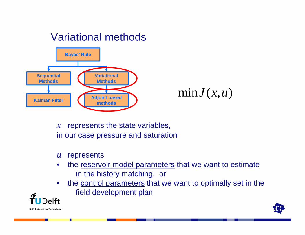
Variational methodsBayes’ Rule
SequentialMethods
VariationalMethods
Kalman Filter Adjoint based methods
),(min uxJ
x represents the state variables, in our case pressure and saturation
u represents• the reservoir model parameters that we want to estimate
in the history matching, or• the control parameters that we want to optimally set in the
field development plan

Variational methods – the principle
)(min xJ

Derivatives with respect to the state variables
Variational methods – the Jacobian, the malefactor
ux
xJ
uJ
duuxdJ
),(
Derivatives with respect to the parameters
T
duuxdJ
),(
adjoint
• We need to calculate the gradient (Jacobian)
• u may easily represent 100s of variables, but worse• x may represent millions of variables, for each time step!
• Options to calculate the Jacobian:• Numerical differentiation: computationally not feasible in our case• Adjoint method: computationally efficient, but
requires significant programming efforts

Challenges
• …
29

30

31

Case studies – Highly nonlinear dynamics
2D variables (400 x 600 grid cells)
-Barotropicpressure-u/v velocity -ice concentration -ice thickness
3D variables (400 x 600 x 22 grid cells)
-Temperature-salinity-u/v current-layer thickness
TOTAL: 27.600.000 variables
Sea level anomalies (satellite, radar altimeters)
-Non linear function of state variables-100.000 observations every week
Sea-surface temperature (satellite, optical)
- 8.000 observations every week
Sea-ice concentrations (satellite, microwave)
- 40.000 observations every week
TOTAL: 148.000 measurements

Global Environmental Multiscale (GEM) Forecasting & Modelling System
2011-2021
Regional and Mesoscale Forecast( 24-48 h, 10-15 km )
& Data assimilation
Medium-range Forecast ( 240 h, 10 to 35 km )
& Data assimilation
Middle Atmosphere Model&
Data assimilation
Regional Climate Model
Monthly Forecast
Multi- Seasonal Forecast
Ensemble Forecast
Limited-Area Model 0-24h 1-2.5km
& Data assimilation
S P A C E
S C A L E
TIME SCALE
Micro-meteorology (10m-1km)
An unified numerical weather forecasting operational system
Canadian Meteorological Center, Weather prediction Division

Reservoir management workflow benchmark study
• Synthetic case
• 44500 active grid cells with 4 values in each grid
• relative perms, initial OWC, vertical transmissibility
• 10 or 20 year production history
• 20 producers and 10 injectors
• time-lapse seismic
Peters et al., 2010, SPE J.
Can we optimize the oil production (maximize NPV) over 30 years period?

Reservoir management workflow benchmark study
Estimation of different propertiesNon-linear dynamicsTwo distinct data typesDifferent simulators used by the participants
Successes:
Use of the EnKF as a history matching method was a common factor among the best performers
Updating models and production strategies more frequently improves the forecast of the final realized NPV.

Seismic History Matching of Fluid Fronts
• Synthetic case based on Brugge field
• 20000 active grid cells with 2 values in each grid cell
•14 years of production
• 17 producers and 10 injectors
• a re-parameterization of time-lapse seismic into front arrivals times (no extra inversion required)
What is the added values of a new parameterization for time –lapse seismic?
Trani et al. 2011, submitted to SPE Journal

Non-linear dynamics
Two distinct data types
MORES simulator
Successes:
The new re-parameterization is a success
No extra inversion required
Improved match for both production and seismic data => improved forecast skills
Seismic History Matching of Fluid Fronts

Roswinkel Field CaseJoint HM subsidence and well data
• Heavily faulted gas field in NE-Netherlands
• 35 possible compartments• GIIP 24.6 bcm• Production period 1980-2005• 9 leveling subsidence campaigns• Max. subsidence 17 cm
Wilschut et al., SPE 141690
Can we identify compartmentalization based on both subsidence and production data?

• Estimation of fault properties
• Moderately non-linear• Two distinct data types• Simulator: IMEX coupled
with geomechanical model
Successes:• Added value of second data
type• EnKF can also be used as
diagnostic tool
Roswinkel Field CaseJoint HM subsidence and well data

Infrared remote sensing of atmospheric composition and air quality: towards operational applications


Conclusions
• Combination between the model and measurements
• Estimation and forecast tool under uncertainties.
• It is very sensitive to the right description of the uncertainties
• Data assimilation is a successful recipe/solution for a lot of different types of applications