Data Analysis with MATLAB - Cornell University … · Data Analysis with MATLAB Steve Lantz Senior...

Data Analysis with MATLAB

Steve Lantz

Senior Research Associate

Cornell CAC

Workshop: Data Analysis on Ranger, January 19, 2012

1/19/2012 www.cac.cornell.edu 2

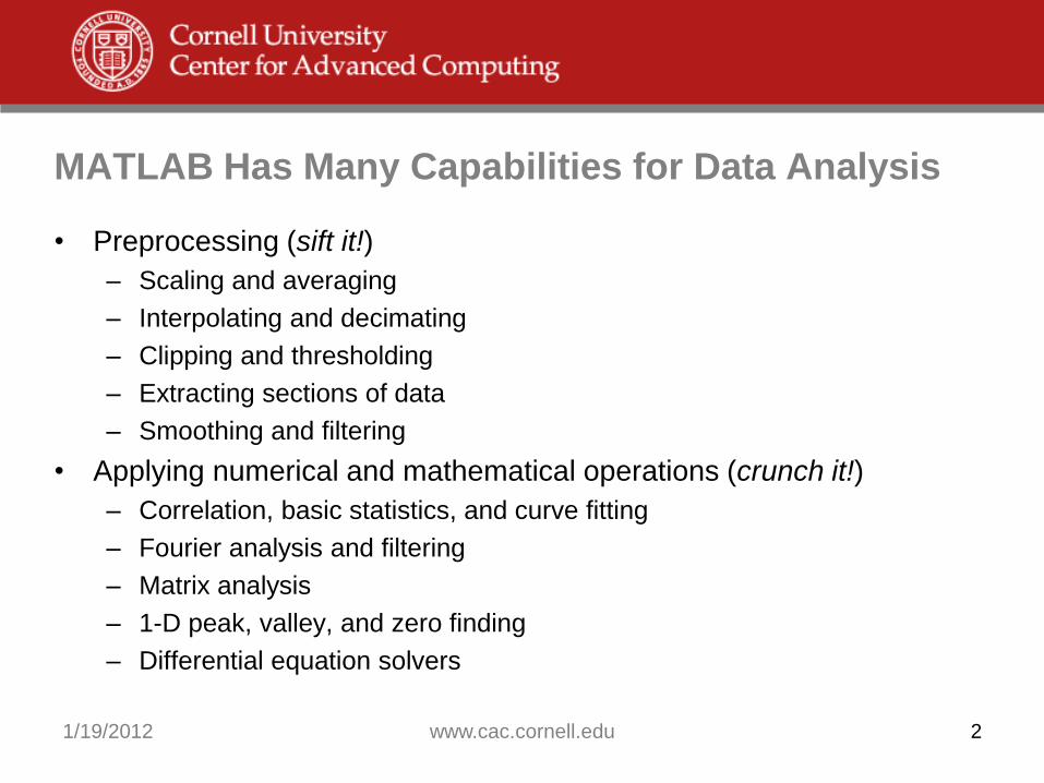
MATLAB Has Many Capabilities for Data Analysis

• Preprocessing (sift it!)

– Scaling and averaging

– Interpolating and decimating

– Clipping and thresholding

– Extracting sections of data

– Smoothing and filtering

• Applying numerical and mathematical operations (crunch it!)

– Correlation, basic statistics, and curve fitting

– Fourier analysis and filtering

– Matrix analysis

– 1-D peak, valley, and zero finding

– Differential equation solvers


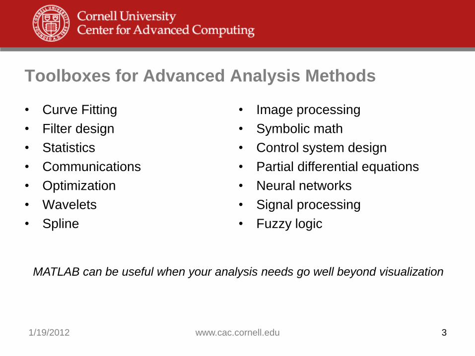
Toolboxes for Advanced Analysis Methods

• Curve Fitting

• Filter design

• Statistics

• Communications

• Optimization

• Wavelets

• Spline

• Image processing

• Symbolic math

• Control system design

• Partial differential equations

• Neural networks

• Signal processing

• Fuzzy logic

MATLAB can be useful when your analysis needs go well beyond visualization


Workflow for Data Analysis in MATLAB

• Access

– Data files - in all kinds of formats

– Software - by calling out to other languages/applications

– Hardware - using the Data Acquisition Toolbox, e.g.

• Pre-process… Analyze… Visualize…

• Share

– Reporting (MS Office, e.g.) - can do this with touch of a button

– Documentation for the Web in HTML

– Images in many different formats

– Outputs for design

– Deployment as a backend to a Web app

– Deployment as a GUI app to be used within MATLAB


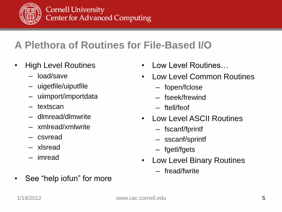
A Plethora of Routines for File-Based I/O

• High Level Routines

– load/save

– uigetfile/uiputfile

– uiimport/importdata

– textscan

– dlmread/dlmwrite

– xmlread/xmlwrite

– csvread

– xlsread

– imread

• See “help iofun” for more

• Low Level Routines…

• Low Level Common Routines

– fopen/fclose

– fseek/frewind

– ftell/feof

• Low Level ASCII Routines

– fscanf/fprintf

– sscanf/sprintf

– fgetl/fgets

• Low Level Binary Routines

– fread/fwrite

Support for Scientific Data Formats

• HDF5 (plus read-only capabilities for HDF4)

– h5disp, h5info, h5read, h5readatt

– h5create, h5write, 5writeatt

• NetCDF (plus similar capabilities for CDF)

– ncdisp, ncinfo, ncread, ncreadatt

– nccreate, ncwrite, ncwriteatt

– netcdf.funcname provides lots of other functionality

• FITS – astronomical data

– fitsinfo, fitsread

• Band-Interleaved Data



Example: Importing Data from a Spreadsheet

• Available functions: xlsread, dlmread, csvread

– To see more options, use the “function browser button” that appears at

the left margin of the command window

• Demo: Given beer data in a .xls file, use linear regression to deduce

the calorie content per gram for both carbohydrates and alcohol

[num,txt,raw] = xlsread('BeerCalories.xls')

y = num(:,1)

x1 = num(:,2)

x2 = num(:,4)

m = regress(y,[x1 x2])

plot([x1 x2]*m,y)

hold on

plot(y,y,'r')


Options for Sharing Results

• Push the “publish” button to create html, doc, etc. from a .m file

– Feature has been around 6 years or so

– Plots become embedded as graphics

– Section headings are taken from cell headings

• Create cells in .m file by typing a %% comment

• Cells can be re-run one at a time in the execution window if desired

• Cells can be “folded” or collapsed so that just the top comment appears

• Share the code in the form of a deployable application

– Simplest: send the MATLAB code (.m file, say) to colleagues

– Use MATLAB compiler to create stand-alone exes or dlls

– Use a compiler add-on to create software components for Java, .NET


Lab: Setting Data Thresholds in MATLAB

• Look over count_nicedays.m in the lab files

– Type “help command” to learn about any command you don’t know

– By default, “dlmread” assumes spaces are the delimiters

– Note, the “find” command does thresholding based on two conditions

– Here, the .* operator (element-by-element multiplication) is doing the job

of a logical “AND”

– Try calling this function in Matlab, supplying a valid year as argument

• Exercises

– Let’s say you love hot weather: change the threshold to be 90 or above

– Set a nicedays criterion involving the low temps found in column 3

– Add a line to the function so it calls “hist” and displays a histogram


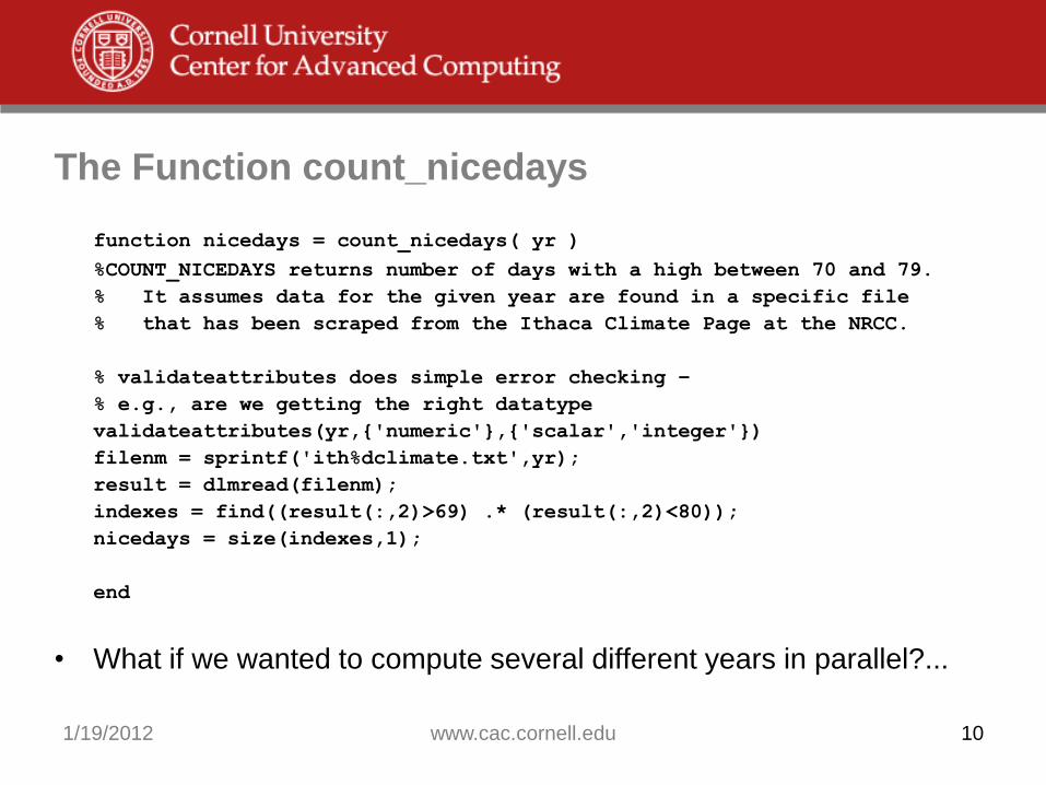
The Function count_nicedays

function nicedays = count_nicedays( yr )

%COUNT_NICEDAYS returns number of days with a high between 70 and 79.

% It assumes data for the given year are found in a specific file

% that has been scraped from the Ithaca Climate Page at the NRCC.

% validateattributes does simple error checking –

% e.g., are we getting the right datatype

validateattributes(yr,{'numeric'},{'scalar','integer'})

filenm = sprintf('ith%dclimate.txt',yr);

result = dlmread(filenm);

indexes = find((result(:,2)>69) .* (result(:,2)<80));

nicedays = size(indexes,1);

end

• What if we wanted to compute several different years in parallel?...


How to Do Parallel Computing in MATLAB

• Core MATLAB already implements multithreading in its BLAS and in

its element-wise operations

• Beyond this, the user needs to make changes in code to realize

different types of parallelism… in order of increasing complexity:

– Parallel-for loops (parfor)

– Multiple distributed runs of a sequential function (createJob)

– Single program, multiple data (spmd, createParallelJob)

– Parallel code constructs and algorithms in the style of MPI

– Codistributed arrays, for big-data parallelism

• The user’s configuration file determines where the workers run

– Parallel Computing Toolbox - take advantage of multicores, up to 8

– Distributed Computing Server - use computer cluster (or local cores)


Access to Local and Remote Parallel Processing


Dividing up a Loop Among Processors

for i=1:3

count_nicedays(2005+i)

end

• Try the above, then try this easy way to spread the loop across

multiple processors (note, though, the startup cost can be high):

matlabpool local 2

parfor i=1:3

count_nicedays(2005+i)

end

• Note, matlabpool starts extra MATLAB workers or “labs” – the size

of the worker pool is set by the default “local” configuration – usually it’s the number of cores (e.g., 2 or 4), but the license allows up to 8


What is parfor Good for?

• It can be used for data parallelism, where each thread works on

independent subsections of a matrix or array

• It can be used for certain kinds of task parallelism, e.g., by doing a

parameter sweep, as in our example (“parameter parallelism?”)

• Either way, all loop iterations must be totally independent

– Totally independent = “embarrassingly parallel”

• Mlint will tell you if a particular loop can't be parallelized

• Parfor is exactly analogous to “parallel for” in OpenMP

– In OpenMP parlance, the scheduling is “guided” as opposed to static

– This means N threads receive many chunks of decreasing size to work

on, instead of simply N equal-size chunks (for better load balance)

A Different Way to Do the Same Thing: createJob

• Try the following code, which runs 3 distributed (independent) tasks

on the local “labs”. The 3 tasks run concurrently, each taking one of

the supplied input arguments.

matlabpool close

sched = findResource('scheduler','configuration','local');

job = createJob(sched)

createTask(job,@count_nicedays,1,{{2006},{2007},{2008}})

submit(job)

wait(job)

getAllOutputArguments(job)

• If only 2 cores are present on your local machine, the 3 tasks will

share the available resources until they finish



How to Do Nearly the Same Thing Without PCT

• Create a MATLAB .m file that takes one or more input parameters

– The parameter may be the name of an input file, e.g.

• Use the MATLAB C/C++ compiler (mcc) to convert the script to a

standalone executable

• Run N copies of the executable on an N-core machine, each with a

different input parameter

– In Windows, this can be done with “start /b”

• For fancier process control or progress monitoring, use a scripting

language like Python

• This technique can even be extended to a cluster

– mpirun can be used for remote initiation of non-MPI processes

– The Matlab runtimes (dll’s) must be available on all cluster machines


Advanced Parallel Data Analysis

• Over 150 MATLAB functions are overloaded for codistributed arrays

– Such arrays are actually split among mutliple MATLAB workers

– In the command window, just type the usual e = d*c;

– Under the covers, the matrix multiply is executed in parallel using MPI

– Some variables are cluster variables, while some are local

• Useful for large-data problems that require distributed computation

– How do we define large? - 3 square matrices of rank 9500 > 2 GB

• Nontrivial task parallelism or MPI-style algorithms can be expressed

– createParallelJob(sched), submit(job) for parallel tasks

– Many MPI functions have been given MATLAB bindings, e.g.,

labSendReceive, labBroadcast; these work on all datatypes

Red Cloud with MATLAB: New Way to Use the PCT

Select the local scheduler –

code runs on client CPUs

Select the CAC scheduler –

Code runs on remote CPUs

MATLAB

Client

MATLAB

Workers

MATLAB

Client

CAC’s client software extends the Parallel Computing Toolbox!

MATLAB Workers

(via Distributed

Computing Server)

MyProxy,

GridFTP


Red Cloud with MATLAB: Services and Security

• File transfer service

– Move files through a GridFTP (specialized FTP) server to a network file

system that is mounted on all compute nodes

• Job submission service

– Submit and query jobs on the cluster (via TLS/SSL); these jobs are to

be executed by MATLAB workers on the compute nodes

• Security and credentials

– Send username/password over a TLS encrypted channel to MyProxy

– Receive in exchange a short-lived X.509 certificate that grants access to

the services


1. Retrieve certificate from MyProxy 2. Upload files to storage via GridFTP 3. Submit job to run MATLAB workers on cluster 4. Download files via GridFTP

MyProxy Server GridFTP Server

HPC 2008 Head Node

DataDirect Networks

9700 Storage

Windows Server 2008

CAC 10Gb Interconnect

Red Cloud with MATLAB: Hardware View

Red Cloud with MATLAB: System Specifications

• Initial configuration: 64 Intel cores in Dell C6100 rack servers

– Total of sixteen 2.4 GHz Xeon E5620 processors (4 cores each)

– 52 cores in Default queue, 4 in Quick queue, 8 in GPU queue

– 2 GB/core in Default and Quick queues; 10 GB/core in GPU queue

• Special feature: 8 NVIDIA Tesla M2070 GPUs (in Dell C410x)

– Each Tesla runs at up to 1 Tflop/s and has 6 GB RAM

• Cluster OS: Microsoft Windows HPC Server 2008 R2

– Supports MATLAB clients on Windows, Mac, and Linux

• Includes 50 GB DataDirect Networks storage (can be augmented)

– RAID-6 with on-the-fly read/write error correction

– Accessible to cores at 1 Gb/s; up to 10 Gb/s externally via GridFTP

• Request an account at http://www.cac.cornell.edu/RedCloud


http://www.cac.cornell.edu/RedCloud/

http://www.cac.cornell.edu/RedCloud/

System Architecture

GridFTP Server

MyProxy Server

Web Server

SQL Server

Compute Nodes NVIDIA

Tesla M2070

Head Node

Dell C410x attached to GPU Nodes

DDN Storage

GPU Nodes

added in 2011

Case Study: Analysis of MRI Brain Scans

• Work by Ashish Raj and Miloš Ivković, Weill-Cornell Medical College

• Research question: Given two different regions of the human brain,

how interconnected are they?

• Potential impact of this technology:

– Study of normal brain function

– Understanding medical conditions that damage brain connections, such

as multiple sclerosis, Alzheimer’s disease, traumatic brain injury

– Surgical planning


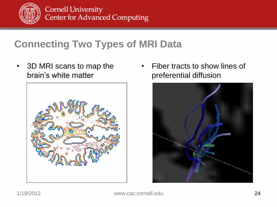
Connecting Two Types of MRI Data

• 3D MRI scans to map the

brain’s white matter

• Fiber tracts to show lines of

preferential diffusion


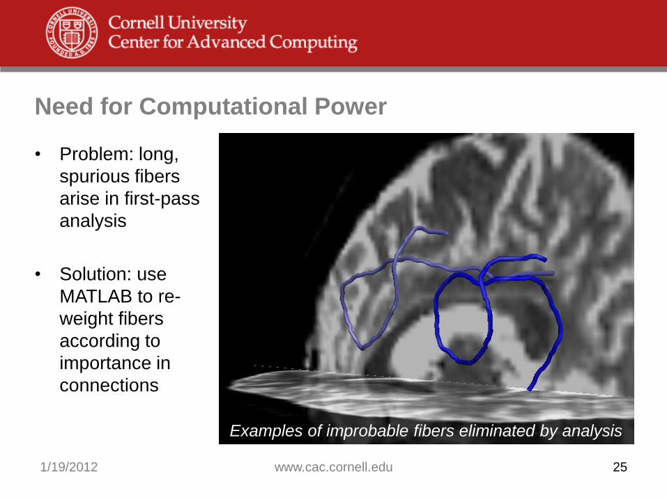
Need for Computational Power

• Problem: long,

spurious fibers

arise in first-pass

analysis

• Solution: use

MATLAB to re-

weight fibers

according to

importance in

connections

Examples of improbable fibers eliminated by analysis


fibers

voxels


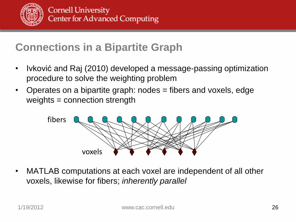
Connections in a Bipartite Graph

• Ivković and Raj (2010) developed a message-passing optimization

procedure to solve the weighting problem

• Operates on a bipartite graph: nodes = fibers and voxels, edge

weights = connection strength

• MATLAB computations at each voxel are independent of all other

voxels, likewise for fibers; inherently parallel

Data Product: Connectivity Matrix

• Graph with 360K

nodes, 1.8M

edges, optimized

in 1K iterations

• The reduced

digraph at right is

based on 116

regions of

interest


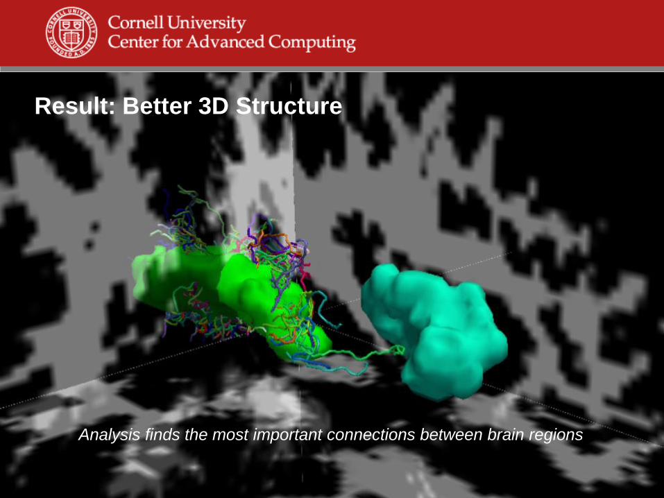
Result: Better 3D Structure

Analysis finds the most important connections between brain regions

fibers

voxels

1. MIN 2. SUM

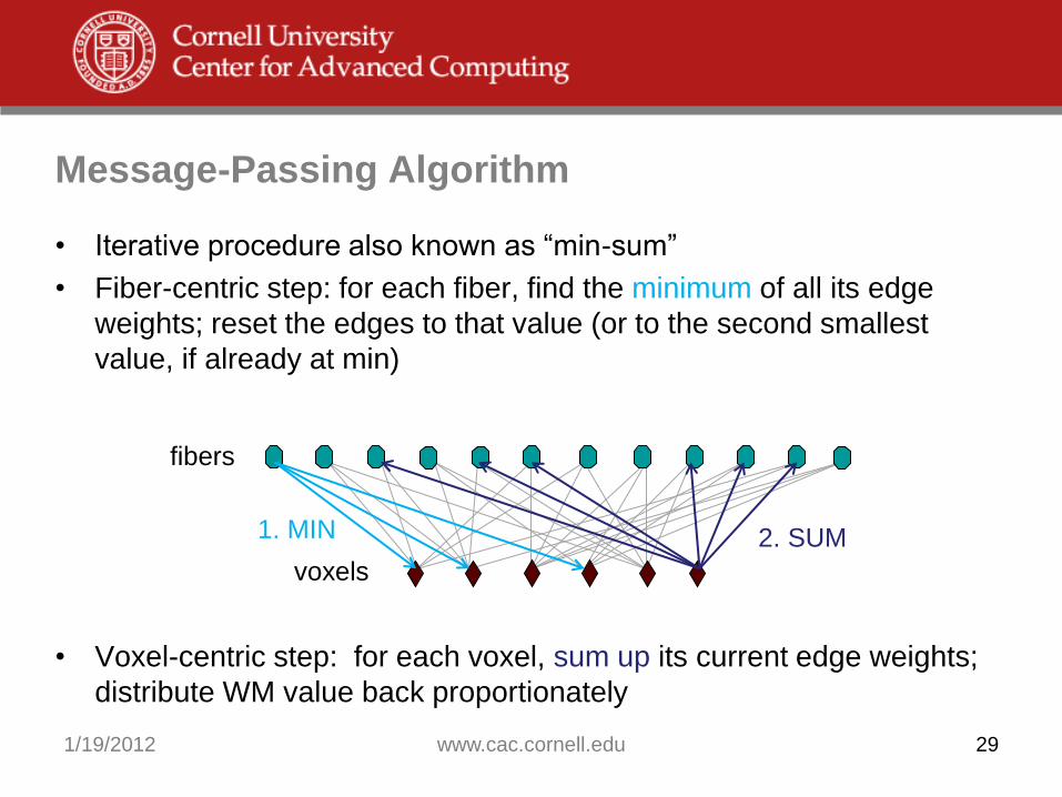
Message-Passing Algorithm

• Iterative procedure also known as “min-sum”

• Fiber-centric step: for each fiber, find the minimum of all its edge

weights; reset the edges to that value (or to the second smallest

value, if already at min)

• Voxel-centric step: for each voxel, sum up its current edge weights;

distribute WM value back proportionately


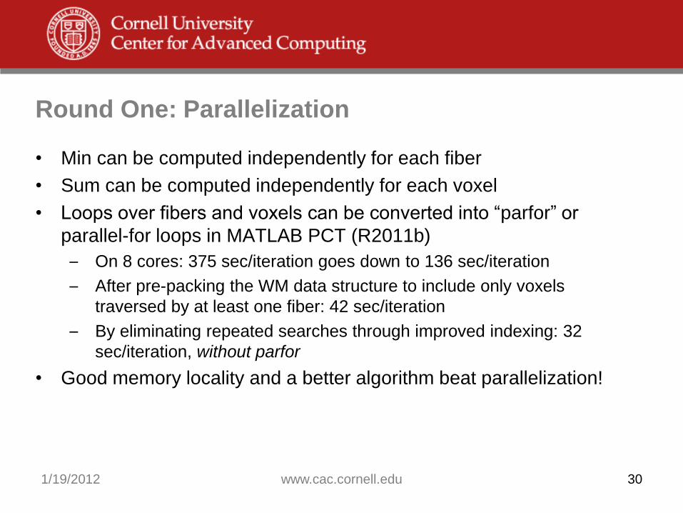
Round One: Parallelization

• Min can be computed independently for each fiber

• Sum can be computed independently for each voxel

• Loops over fibers and voxels can be converted into “parfor” or

parallel-for loops in MATLAB PCT (R2011b)

– On 8 cores: 375 sec/iteration goes down to 136 sec/iteration

– After pre-packing the WM data structure to include only voxels

traversed by at least one fiber: 42 sec/iteration

– By eliminating repeated searches through improved indexing: 32

sec/iteration, without parfor

• Good memory locality and a better algorithm beat parallelization!


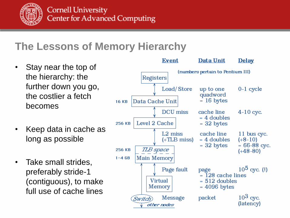
The Lessons of Memory Hierarchy

• Stay near the top of

the hierarchy: the

further down you go,

the costlier a fetch

becomes

• Keep data in cache as

long as possible

• Take small strides,

preferably stride-1

(contiguous), to make

full use of cache lines

MATLAB Loves Matrices

• Original code was written using structs

– Advantage: little wasted space; handles variable-length lists of edges

connected to a voxel (1–274) or fiber (2–50)

– Disadvantage: poor data locality, because structs hold lots of

extraneous info about voxels/fibers

– Disadvantage: unsupported on GPU in MATLAB

• Better to store data in matrices

– Column-wise operations on a matrix are often multithreaded in the

MATLAB core library; no programmer effort required

– Implication: easily get “vectorized” performance on CPUs or GPUs by

converting loops into matrix operations


Round Two: Vectorization

• So, just throw everything into one giant matrix?

– First problem: row-major ordering = bad stride

– Second problem: mixing of dissimilar data = poor data locality

– Due to these problems, the initial matrix-based version of the serial

min-sum algorithm ran slower, 53 sec/iteration

– Yet another lesson of memory hierarchy (for a collaborator)

• First optimization steps were easy…

– Make columns receive all edge weights (messages) pertaining to one

voxel or fiber—MATLAB stores in column-major order

– Pull out only necessary info and store in separate, condensed matrices


Round Three: CPU Optimization

• Tighten up memory utilization by grouping fibers and voxels

according to numbers of coordinating edges

– Different matrices for fibers that connect to 2, 3, 4… edges

– Now have full columns in the matrix for all 2-edge fibers, etc.

– Put the series of matrices into a “cell array” for easy reference

• Resulting code is much more complex

– New inner for-loops over fiber count, voxel count

– Challenge to build the necessary indexing

• Excellent performance in the end: 0.25 sec/iteration

• Good outcome, but days and days of work by Eric Chen


• New feature in MATLAB R2010b: gpuArray datatype, operations

• To use the GPU, MATLAB code changes are trivial

– Move data to GPU by declaring a gpuArray

– Methods like fft() are overloaded to use internal CUDA code on

gpuArrays

• Initial benchmarking with large 1D and 2D FFTs shows excellent

acceleration on 1 GPU vs. 8 CPU cores

– Including communication: up to 10x speedup

– Excluding communication: up to 20x speedup

• Easy and fast… BUT can it help with the particular data analysis?

g = gpuArray(r);

f = fft2(g);


New Idea: GPGPU in MATLAB

GPU Definitely Excels at Large FFTs in MATLAB

• 2D FFT > 8 MB can be 9x faster on GPU (including data transfers),

but array of 1D FFTs is equally fast on 8 cores

• Limited to 256 MB due to bug in cuFFT 3.1; fixed in 3.2


Round Four: GPU Optimization

• In R2011b, min and sum can use MATLAB’s built-in CUDA code!

• Go back to big, simple matrices with top-heavy columns

– Reason 1: GPU doesn’t deal well with nested for-loops

– Reason 2: Want vectorized or SIMD operations on millions of items

• Resulting code is actually less complex

– Keep data in a few huge arrays

– Move them to the GPU with gpuArray()

– Functions min and sum are overloaded (polymorphic), so no further

code changes are needed

• Best result (after a few tricks): 0.15 sec/iteration

– 350x speedup over initial matrix-based version

– 2500x speedup over initial struct-based version


Is It Really That Simple?

• No. The GPU portion of MATLAB PCT is evolving rapidly.

– A year ago, the move to GPU was impossible: subscripting into arrays

wasn’t allowed, min was completely absent, etc.

– Now these operations are present and work well, but gaps still remain;

e.g., min does not return the location of the minima as it does on the

CPU, and a workaround was needed for the GPU.

• Your application must meet two important criteria.

– All required operations must be implemented natively for type

GPUArray, so your data seldom have to leave the GPU.

– The overall working dataset must be large enough to exploit 100s of

thread processors without exceeding GPU memory.


Implications for Data Analysis in MATLAB

• The MATLAB Parallel Computing Toolbox has a variety of features

that can dramatically speed up the analysis of large datasets

• New GPU functionality is a good addition to the arsenal

• A learning curve must be climbed…

– General knowledge of parallel and vector computing can be helpful for

restructuring the compute-intensive portions of a code

– Specific knowledge of PCT functions is needed to exploit features

• But speed matters!…

– MRI image analysis has mostly been of interest to medical researchers

– Now it can potentially move into the realm of a diagnostic tool for real-

time, clinical use

– Modest hardware requirements may make such computations feasible


Data Analysis with MATLAB - Cornell University … · Data Analysis with MATLAB Steve Lantz Senior...

Documents

Transcript of Data Analysis with MATLAB - Cornell University … · Data Analysis with MATLAB Steve Lantz Senior...