1

Data Analysis Using Spark and Sparkling Water J. Zhang

School of Computing, Queen's university Kingston, Ontario

Canada 12jnz@queensu.ca

ABSTRACT The term “big data” is used to describe huge volume of data produced and generated with a rapid rate from various sources. Big data

analytics examines large amounts of data to extract hidden patterns, correlations and other insights. It is used in almost every field such as spotting business trends, preventing diseases, combating crime and so on. Machine learning techniques are ideal for exploiting the value and opportunities hidden behind data. While traditional techniques used to process data on a single machine are not able to provide an efficient way to store or analyze massive data, big data processing frameworks take the responsibility and provide high availability using cluster computing. This paper introduces Sparkling Water which is an integration of a general purposed big data framework called Spark, and a powerful machine learning library called H2O.ai. Sparkling water combines H2O’s machine learning capabilities with Spark’s unified in-memory data processing engine. This paper provides three experiments. The first two experiments demonstrate how to preform predictive analytics with Sparkling Water. The last experiment shows the way of using random forest algorithm imported from Spark primitive library, MLlib for predictive analytics. Sparkling Water is found to be an easier way for applying machine learning since it offers a user-friendly web GUI to enhance its accessibility for users without programing experience.

KEYWORDS Big data analytics, Machine learning, Spark, MLlib, H2O.ai

1 INTRODUCTION In the big data era, huge volume of data are produced and generated with a rapid rate from various sources such as smart phone, sensor

measurements, and social media. Analysis of big data extracts potential value from data. Big data analytics such as predictive analytics and user behavior analytics can be used to spot business trends, prevent diseases, combat crime and so on. In the analytics, machine learning is ideal for exploiting the value and opportunities hidden behind big data. It can used to find relationships or structure between different inputs and identify the likelihood of future outcomes based on historical data. While traditional techniques used to process data on a single machine are not able to provide an efficient way to store or analyze these massive data, big data processing frameworks take the responsibility and provide high availability using cluster computing.

Apache Spark [1] is one of the most popular and advanced big data frameworks. Recently, this general-purpose framework is regarded as the next generation of big data analysis paradigms. It was developed in AMPLab of University of California at Berkeley and open sourced by Apache. The main abstraction in Spark is resilient distributed dataset (RDD), which is a read-only collection of partitioned records. An RDD is created through transformations on data in stable storage or on other RDDs. All transformations of RDDs are logged in a lineage stored in drive. Using lazy evaluations, RDDs are not always materialized in order to save memory space. The lineage provides enough information to compute an RDD from data in stable storage when it is needed for an action. Because of this major unique feature, Spark is able to process data in-memory up to 100 times faster than Hadoop MapReduce [1]. Moreover, Spark is integrated in various common programing languages such as Java, Python, and Scala. It powers a set of core libraries used for processing both streaming and batch data, supporting more languages such as SQL and R, and suiting a wider range of applications including machine learning and graphic analytics. Spark’s native machine learning library, MLlib [2], contains common machine learning algorithms including classification regression, clustering and collaborative filtering, and also some utilities including linear algebra, statistic and data handling.

H2O.ai [2] is an intelligent open source machine-learning library for big data analytics. Its benefits include support for all common databases and file types, easy-to-use Web User Interface, real-time data scoring and massively scalable big data analysis. It can be integrated with other systems such as R, RStudio, Storm and Spark as a third party machine-learning library. The combination of Spark and H2O.ai is called Sparkling Water [4], allowing Spark’s data manipulation capabilities to be used with H2O’s fast and scalable machine learning models. Moreover, H2O offers a Web GUI called H2O Flow to build and evaluate models visually. Therefore, it is a simple and ideal machine learning platform for data scientists as well as someone who is not expert at coding.

The next section reviews terminologies used in this paper such as principles of supervised and unsupervised learning and some widely used machine learning models for each of them. Section 3 introduces all pre-requisites required by Spark and Sparkling Water as well as their functions. In section 4, the first two experiments demonstrate how to analyze and classify data by applying machine learning models using Sparkling Water. The last experiment demonstrates the analysis progress using Spark. Section 5 summarizes experience of using both H2O and MLlib with Spark, and indicates some future work.

2

2 TERMINOLOGY Machine learning is a data analysis method used to automatically apply complex mathematical calculations, finding hidden insights

from massive data. Generally, machine learning is divided into two types: supervised and unsupervised. In supervised learning, the outputs are provided and used to train a machine learning model in order to generate reasonable outputs. In unsupervised learning, no output is provided, so machine clusters or matches inputs into different classes using specific algorithms. There are hundreds of different machine learning algorithms. Several popular machine learning algorithms are described under the section 2.1 for supervised learning and section 2.2 for unsupervised learning. Section 2.3 describes a general purpose model called deep learning.

2.1 Supervised Learning Supervised learning [5] requires prior knowledge to compute outcomes. In other words, historical data are essential to this type of

analysis. In the dataset, a label attribute is considered as output of the learning algorithm and the other attributes are considered as features or inputs. A supervised learning algorithm trains a model by learning from inputs and finding a function or a rule to get the outputs. Then, the model can be built on new inputs in order to compute outputs. It is commonly used for prediction and classification analysis. Four widely used supervised learning algorithms, distributed random forests, gradient boosting method, generalized linear modeling and Naïve Bayes, are described in section 2.1.1, 2.1.2, 2.1.3 and 2.1.4 respectively.

2.1.1 Distributed Random Forests. Random Forests [6] is one of the most accurate and popular classification algorithms. It is a supervised machine learning model. Training many decision trees, it takes the average across the trees to develop a prediction. It can handle thousands of input variables without variable deletion and missing values, as well as work for variable selection by computing variable importance. However, the classifications made by Random Forests might be difficult for humans to interpret.

2.1.2 Gradient Boosting Method (GBM). Gradient Boosting Method [7] is a supervised machine learning model that produces a prediction model by training a sequence of decision tress and generalizes them by allowing optimization. It can model interactions and non-linear features, but might generate too many trees and lead to overfitting.

2.1.3 Generalized Linear Modeling (GLM). Generalized Linear Modeling [8] is a supervised machine learning model. It is a flexible form of linear regression. All features are considered as measurements. Label attribute is considered as the response variable. The model can find a linear function to link measurements and response variable. Each measurement has a magnitude of variance. In other words, the response variable can be simply predicted by computing the link function. GLM combines classical statistics with the most advanced machine learning. It is one of the fastest models but its prerequisite is to assume that there is a linear relation among the attributes selected. In other words, GLM algorithm only operates on numeric attributes. Moreover, it sometimes doesn’t work very well when there are too many attributes.

2.1.4 Naïve Bayes. Naïve Bayes [10] is a supervised learning model which is widely used as a classifier. It has an assumption: evidence splits into parts that are independent. If the assumption holds, the Naïve Bayes classifier will converge quicker than discriminative models. Its response variable must be a category. It works well with small datasets but not with large datasets. Sometimes, its assumption is constraining.

2.1 Unsupervised Learning Unsupervised leaning [5] is used when there is no prior knowledge about a specific output to provide some insight from the data by

finding the most unusual sets of data among the dataset. For example, to predict which transactions are frauds, data scientists might use machine learning to identify those unusual transactions comparing to all the other transactions, and might flag these for further investigation. Another user case is customer segmentations. Machine learning finds some patterns according to personal information or other data collected, and segments customers into several groups. Four widely used unsupervised learning algorithms, k-means, principal components analysis, and generalized low rank models are described in section 2.2.1, 2.2.2, and 2.2.3 respectively.

2.2.1 K-means. K-means [9] is one of the most widely used unsupervised clustering algorithms. K-means stores k centroids defined by users, one for each cluster. An observation is considered to be in a particular cluster if it is closer to that cluster's centroid than any other centroids. In other words, K-means algorithm partitions observations in a dataset into k clusters according to the similarity. This kind of clusters is non-hierarchical, so they won’t overlap. With a large number of variables, k-means may compute faster and produce tighter clusters than hierarchical clustering. However, it is difficult to define the most appropriate k value and compare the quality of the clusters produced.

2.2.2 Principal Components Analysis (PCA). Principal Components Analysis (PCA) [11] is an unsupervised algorithm that is used for doing dimension reduction. It evaluates a set of raw features and reduces them into indices that are independent of one another. The advantage is that it can deal with large datasets of both objects and variables, but it only supports numeric data. Moreover, it is not suitable to use if all the components have a high variance.

2.2.3 Generalized Low Rank Models (GLRM). The Generalized Low Rank Model (GLRM) [12] is a new unsupervised machine learning method for reconstructing missing values and identifying important features in heterogeneous data. GLRMs are an extension of matrix factorization methods such as PCA. Unlike PCA, GLRM supports all data types. It can handle mixed numeric, Boolean, ordinal data even with a bunch of missing values.

3

2.3 Deep Learning Deep Learning [13] is a general-purpose model. It models high-level patterns often based on artificial neural networks. Unlike the

“normal” neural networks that can only do supervised prediction and classification, Deep Learning can do both unsupervised and supervised learning tasks. However, it requires lots of data for high accuracy and expensive computation.

3 EXPERIMENT ENVIRONMENT Prerequisites of the newest version of Sparkling Water are Java version 1.6 or newer, Scala 2.11, and Spark of pre-build for Hadoop 2.4

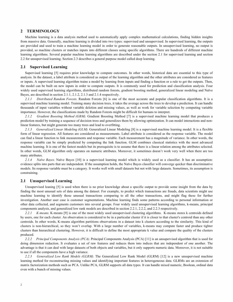
and later. The installation of Spark and Sparkling Water is described straightforwardly on their website. The default port to Spark UI is 4040. The Spark web UI provides a list of scheduler stages and tasks, a summary of RDD sizes and memory usage, environmental information, and information about the running executors. It allows users to inspect job executions in the SparkContext or H2OContext with Spark-shell using a browser. Unlike H2O Flow, users cannot do any execution with the Spark web UI.

Figure 1 Spark UI

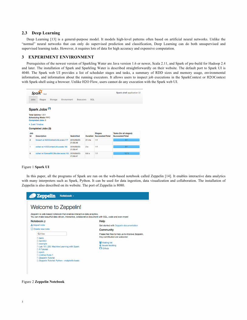
In this paper, all the programs of Spark are run on the web-based notebook called Zeppelin [14]. It enables interactive data analytics with many interpreters such as Spark, Python. It can be used for data ingestion, data visualization and collaboration. The installation of Zeppelin is also described on its website. The port of Zeppelin is 8080.

Figure 2 Zeppelin Notebook

4

The default port to the H2O Flow UI is 54321. H2O Flow is an easy-to-use notebook-style user web interface. It combines code execution, plots, and so on. With H2O Flow, users can import files, build models, make predictions and iteratively improve them. Its interface is composed of executable cells. Each cell can be considered as an input box. User can enter commands, define functions, and run existing functions in cells. Executing cells produces outputs that are graphical objects with different options such as ‘inspect’ to view detailed results depending on which execution is done. The Admin menu allows users to view the cluster status, a timeline of events, CPU status and logs to troubleshoot issues.

Figure 3 H2O Flow

4 EXPERIMENTS Experiment 4.1 and 4.2 provide two examples of using Sparkling Water to perform a regression and a classification analysis.

Experiment 4.3 demonstrates the way of using random forest algorithm imported from Spark primitive library, MLlib for predictive analytics. The two datasets used for experiments are both retrieved from UCI Machine Learning Repository [15, 16].

4.1 Analysis using Sparkling Water for Default of credit card clients Data Set [15] This dataset took the credit payment data from a bank in Taiwan.

Figure 4 Data selected from default of credit card clients dataset [15]

The binary variable Y is a response column, representing the default payment (1: Yes, 0: No). The 23 explanatory variables is described below:

1. X1: Amount of the given credit (NT dollar): it includes both the individual consumer credit and his/her family (supplementary) credit.

2. X2: Gender (1 = male; 2 = female).

5

3. X3: Education (1 = graduate school; 2 = university; 3 = high school; 4 = others). 4. X4: Marital status (1 = married; 2 = single; 3 = others). 5. X5: Age (year). 6. X6 - X11: History of past payment. We tracked the past monthly payment records (from April to September, 2005) as follows:

X6 = the repayment status in September, 2005; X7 = the repayment status in August, 2005; . . .;X11 = the repayment status in April, 2005. The measurement scale for the repayment status is: -1 = pay duly; 1 = payment delay for one month; 2 = payment delay for two months; . . .; 8 = payment delay for eight months; 9 = payment delay for nine months and above.

7. X12-X17: Amount of bill statement (NT dollar). X12 = amount of bill statement in September, 2005; X13 = amount of bill statement in August, 2005; . . .; X17 = amount of bill statement in April, 2005.

8. X18-X23: Amount of previous payment (NT dollar). X18 = amount paid in September, 2005; X19 = amount paid in August, 2005; . . .;X23 = amount paid in April, 2005.

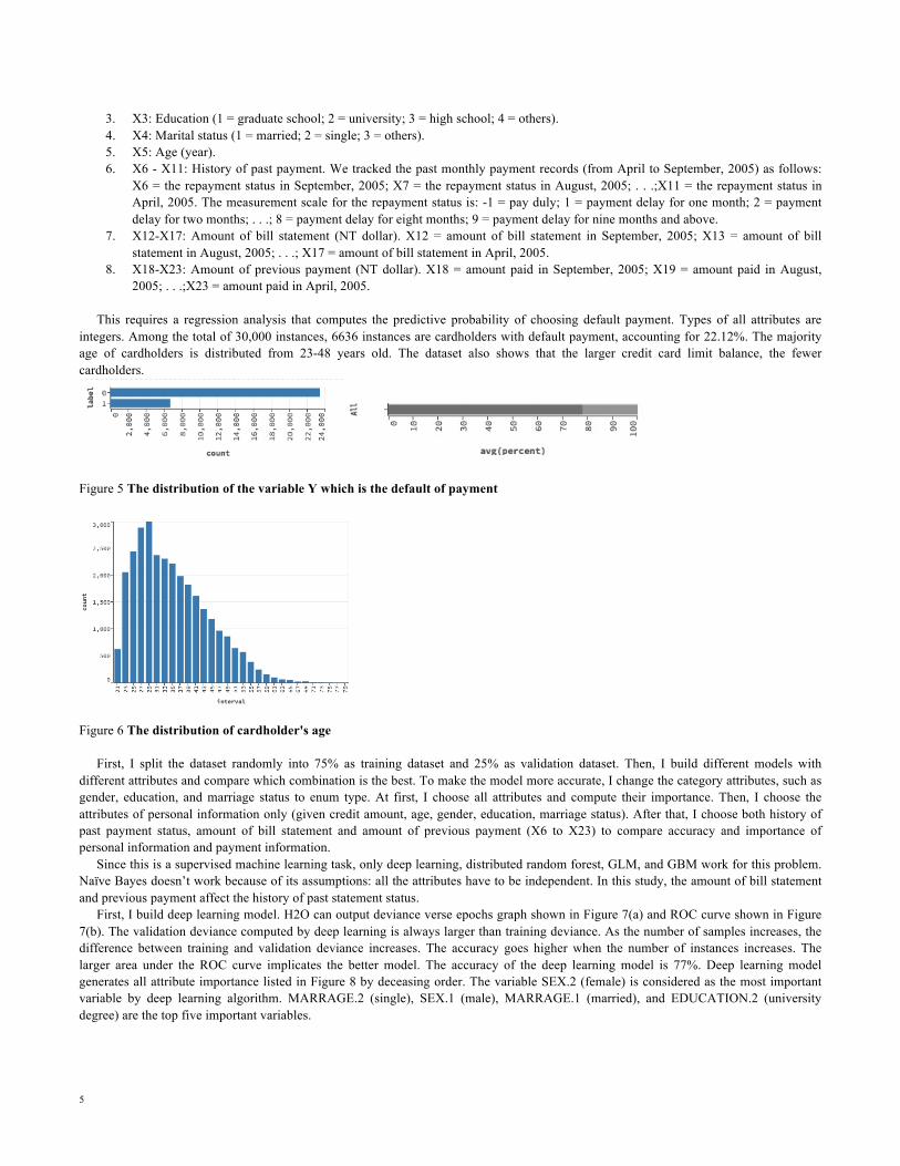
This requires a regression analysis that computes the predictive probability of choosing default payment. Types of all attributes are

integers. Among the total of 30,000 instances, 6636 instances are cardholders with default payment, accounting for 22.12%. The majority age of cardholders is distributed from 23-48 years old. The dataset also shows that the larger credit card limit balance, the fewer cardholders.

Figure 5 The distribution of the variable Y which is the default of payment

Figure 6 The distribution of cardholder's age

First, I split the dataset randomly into 75% as training dataset and 25% as validation dataset. Then, I build different models with different attributes and compare which combination is the best. To make the model more accurate, I change the category attributes, such as gender, education, and marriage status to enum type. At first, I choose all attributes and compute their importance. Then, I choose the attributes of personal information only (given credit amount, age, gender, education, marriage status). After that, I choose both history of past payment status, amount of bill statement and amount of previous payment (X6 to X23) to compare accuracy and importance of personal information and payment information.

Since this is a supervised machine learning task, only deep learning, distributed random forest, GLM, and GBM work for this problem. Naïve Bayes doesn’t work because of its assumptions: all the attributes have to be independent. In this study, the amount of bill statement and previous payment affect the history of past statement status.

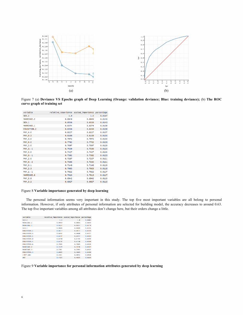
First, I build deep learning model. H2O can output deviance verse epochs graph shown in Figure 7(a) and ROC curve shown in Figure 7(b). The validation deviance computed by deep learning is always larger than training deviance. As the number of samples increases, the difference between training and validation deviance increases. The accuracy goes higher when the number of instances increases. The larger area under the ROC curve implicates the better model. The accuracy of the deep learning model is 77%. Deep learning model generates all attribute importance listed in Figure 8 by deceasing order. The variable SEX.2 (female) is considered as the most important variable by deep learning algorithm. MARRAGE.2 (single), SEX.1 (male), MARRAGE.1 (married), and EDUCATION.2 (university degree) are the top five important variables.

6

(a) (b)

Figure 7 (a) Deviance VS Epochs graph of Deep Learning (Orange: validation deviance; Blue: training deviance); (b) The ROC curve graph of training set

Figure 8 Variable importance generated by deep learning

The personal information seems very important in this study. The top five most important variables are all belong to personal information. However, if only attributes of personal information are selected for building model, the accuracy decreases to around 0.63. The top five important variables among all attributes don’t change here, but their orders change a little.

Figure 9 Variable importance for personal information attributes generated by deep learning

7

Selecting only history of past payment status (attributes X6-X23), the deep learning model provides a 0.76 accuracy which is lower than selecting all attributes but higher than only considering the personal information. In other words, payment information is more important than personal information in this example.

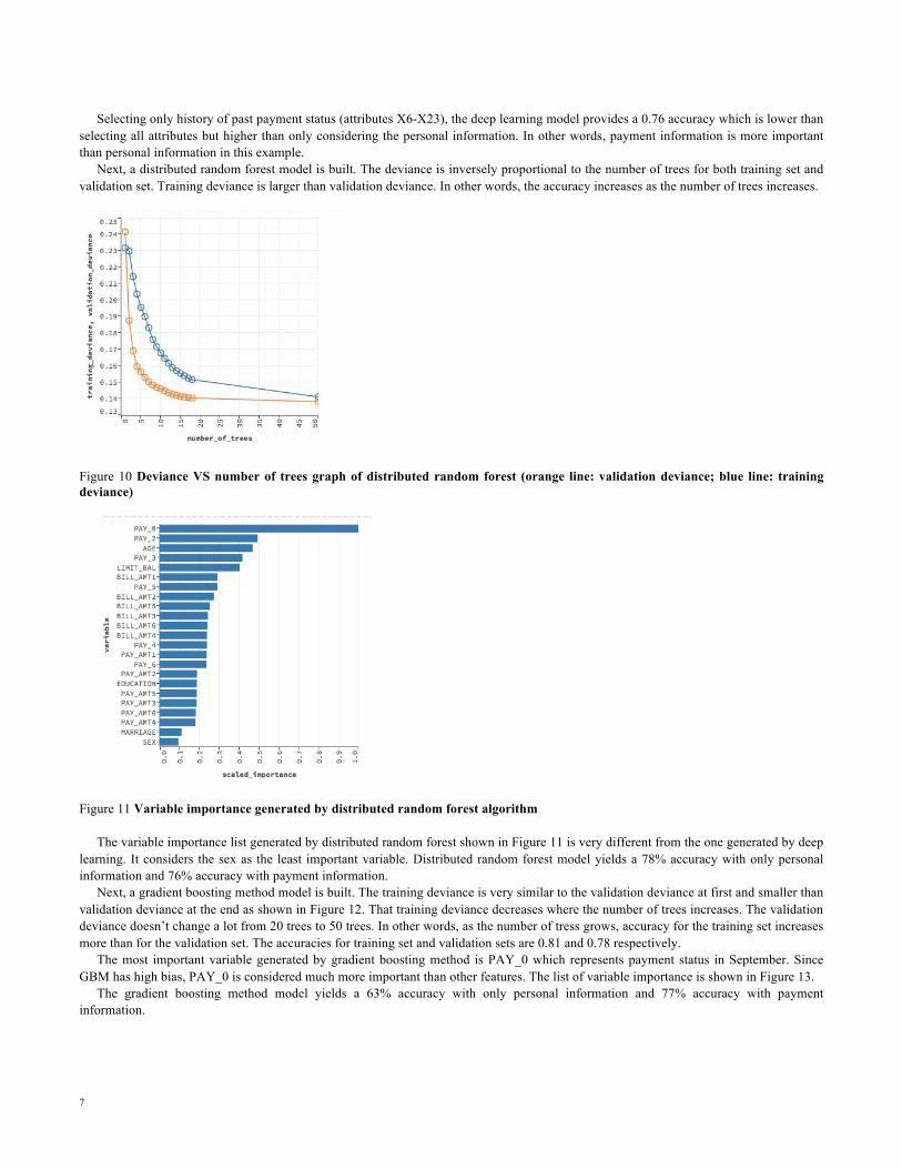
Next, a distributed random forest model is built. The deviance is inversely proportional to the number of trees for both training set and validation set. Training deviance is larger than validation deviance. In other words, the accuracy increases as the number of trees increases.

Figure 10 Deviance VS number of trees graph of distributed random forest (orange line: validation deviance; blue line: training deviance)

Figure 11 Variable importance generated by distributed random forest algorithm

The variable importance list generated by distributed random forest shown in Figure 11 is very different from the one generated by deep learning. It considers the sex as the least important variable. Distributed random forest model yields a 78% accuracy with only personal information and 76% accuracy with payment information.

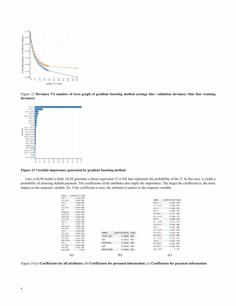
Next, a gradient boosting method model is built. The training deviance is very similar to the validation deviance at first and smaller than validation deviance at the end as shown in Figure 12. That training deviance decreases where the number of trees increases. The validation deviance doesn’t change a lot from 20 trees to 50 trees. In other words, as the number of tress grows, accuracy for the training set increases more than for the validation set. The accuracies for training set and validation sets are 0.81 and 0.78 respectively.

The most important variable generated by gradient boosting method is PAY_0 which represents payment status in September. Since GBM has high bias, PAY_0 is considered much more important than other features. The list of variable importance is shown in Figure 13.

The gradient boosting method model yields a 63% accuracy with only personal information and 77% accuracy with payment information.

8

Figure 12 Deviance VS number of trees graph of gradient boosting method (orange line: validation deviance; blue line: training deviance)

Figure 13 Variable importance generated by gradient boosting method

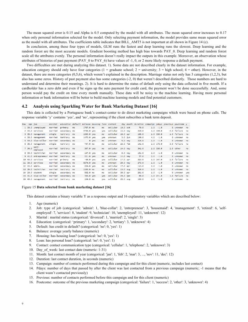
Last, a GLM model is built. GLM generates a linear regression Y=a+bX that represents the probability of the Y. In this case, it yields a probability of choosing default payment. The coefficients of the attributes also imply the importance. The larger the coefficient is, the more impact on the response variable. So, if the coefficient is zero, the attribute is useless to the response variable.

(a) (b) (c)

Figure 14 (a) Coefficients for all attributes; (b) Coefficients for personal information; (c) Coefficients for payment information

9

The mean squared error is 0.15 and Alpha is 0.5 computed by the model with all attributes. The mean squared error increases to 0.17 when only personal information selected for the model. Only selecting payment information, the model provides same mean squared error as the model with all attributes. The coefficients table indicates that BILL_AMT5 is not important at all shown in Figure 14 (c).

In conclusion, among these four types of models, GLM runs the fastest and deep learning runs the slowest. Deep learning and the random forest are the most accurate models. Gradient boosting method has high bias towards PAY_0. Deep learning and random forest scale all the attributes evenly. The personal information doesn’t really impact the outputs in this example. Moreover, an observation whose attributes of histories of past payment (PAY_0 to PAY_6) have values of -1, 0, or 2 more likely response a default payment.

Two difficulties are met during analyzing this dataset. 1). Some data are not described clearly in the dataset information. For example, education category should only have four categories (1 = graduate school; 2 = university; 3 = high school; 4 = other). However, in the dataset, there are more categories (0,5,6), which weren’t explained in the description. Marriage status not only has 3 categories (1,2,3), but also has some zeros. History of past payment also has some categories (-2, 0) that weren’t described distinctly. Those numbers are hard to understand and determine their meanings. 2). It is hard to determine the status of default only using the data collected in five month. If a cardholder has a zero debt and even if he signs up the auto payment for credit card, the payment won’t be done successfully. And, some person would pay the credit on time every month manually. These data will be noisy to the machine learning. Having more personal information or bank information will be better to build machine learning models and find potential customers.

4.2 Analysis using Sparkling Water for Bank Marketing Dataset [16] This data is collected by a Portuguese bank’s contact-center to do direct marketing campaigns which were based on phone calls. The

response variable ‘y’ contains ‘yes’, and ‘no’, representing if the client subscribes a bank term deposit.

Figure 15 Data selected from bank marketing dataset [16]

This dataset contains a binary variable Y as a response output and 16 explanatory variables which are described below:

1. Age (numeric) 2. Job: type of job (categorical: 'admin': 1, 'blue-collar': 2, 'entrepreneur': 3, 'housemaid': 4, 'management': 5, 'retired': 6, 'self-

employed': 7, 'services': 8, 'student': 9, 'technician': 10, 'unemployed': 11, 'unknown': 12) 3. Marital : marital status (categorical: 'divorced': 1, 'married': 2, 'single': 3) 4. Education: (categorical: ‘primary': 1, 'secondary': 2, 'tertiary': 3, 'unknown': 4) 5. Default: has credit in default? (categorical: 'no': 0, 'yes': 1) 6. Balance: average yearly balance (numeric) 7. Housing: has housing loan? (categorical: 'no': 0, 'yes': 1) 8. Loan: has personal loan? (categorical: 'no': 0, 'yes': 1) 9. Contact: contact communication type (categorical: 'cellular': 1, 'telephone': 2, 'unknown': 3) 10. Day_of_week: last contact date (numeric: 1-31) 11. Month: last contact month of year (categorical: 'jan': 1, 'feb': 2, 'mar': 3, ..., 'nov': 11, 'dec': 12) 12. Duration: last contact duration, in seconds (numeric) 13. Campaign: number of contacts performed during this campaign and for this client (numeric, includes last contact) 14. Pdays: number of days that passed by after the client was last contacted from a previous campaign (numeric; -1 means that the

client wasn’t contacted previously) 15. Previous: number of contacts performed before this campaign and for this client (numeric) 16. Poutcome: outcome of the previous marketing campaign (categorical: 'failure': 1, 'success': 2, 'other': 3, 'unknown': 4)

10

Age, job, marital, education, default, housing loan, personal loan are bank client personal information data. Contact type, contact date (month, year), and duration of contact time are campaign data, and the rest of attributes are other information related to this problem. The duration attribute must be the most important attribute. It highly affects the output target because only customers who are interested will be willing to spend time in the communication and subscribe the term deposit. This value is unknown before a call is performed so it should be discarded when building a model for prediction.

In the bank-full.csv, there are 45211 objects in total ordered by date and bank.csv holds 10% of the examples randomly selected from bank-full.csv. There is no any missing value. The percentage of Yes is 12% and No is 88% in the full dataset. Since it is a classification problem and the dataset contains both numeric and string data, only deep learning, distributed random forest and GBM work for it. Naïve Bayes doesn’t work here because the attributes previous and pdays are dependent, contradicting its assumption. If previous is zero, then pdays must be -1.

I split the bank-full dataset into 75% to be the training set and 25% to be the validation set randomly to build models. Then, I use those models to predict the bank dataset to compare the accuracy. Deep Learning algorithm yields a 76% accuracy. Distributed random forest yields a 85% accuracy. Gradient boosting method yields a 79% accuracy.

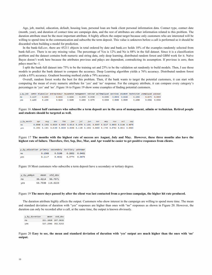
Overall, random forest works the best for this problem. Then, if the bank wants to target the potential customers, it can start with computing the mean of every numeric attribute for ‘yes’ and ‘no’ response. For the category attribute, it can compare every category’s percentages in ‘yes’ and ‘no’. Figure 16 to Figure 19 show some examples of finding potential customers.

Figure 16 Almost half customers who subscribe a term deposit are in the area of management, admin or technician. Retired people and students should be targeted as well.

Figure 17 The months with the highest rate of success are August, July and May. However, these three months also have the highest rate of failure. Therefore, Oct, Sep, Dec, Mar, and Apr would be easier to get positive responses from clients.

Figure 18 Most customers who subscribe a term deposit have a secondary or tertiary degree.

Figure 19 The more days passed by after the client was last contacted from a previous campaign, the higher hit rate produced.

The duration attribute highly affects the output. Customers who show interest in the campaign are willing to spend more time. The mean and standard deviation of duration with “yes” responses are higher than ones with “no” responses as shown in Figure 20. However, the duration can only be recorded after a call, at the same time, the output is known obviously.

Figure 20 Easy to see, the mean and standard deviation of duration with ‘yes’ output are much higher than the ones with ‘no’ output.

11

In summary, age, job, marital, education, contact type, account balance and month attributes have more impact to the output than other attributes. The distributed random forest performs much better and faster than deep learning and GBM. GBM is based on weak learners which have high bias and low variance. Distributed Random Forest is better than GBM in this example because it is based on bagging and uses fully grown decision tress.

4.3 Analysis using Spark and MLlib for Bank Marketing Dataset [16] MLlib is a native Spark machine learning library shipped with Spark as a standard component since Spark 0.8. It provides many widely

used algorithms including SVM, random forest, k-means, and logistic regression. Before Spark 2.0, the default machine learning API was RDD-based in the spark.MLlib package. Now, the primary machine learning API switches to the DataFrame-based API in the spark.ml package. DataFrames provide a user-friendlier API than RDD and more benefits including SQL queries, uniform API across ML algorithms and across multiple languages. This experiment runs on Spark 2.0 and Zeppelin 0.6. It shows how to apply random forest model in Spark.

First step is to import machine learning packages.

A Scala class is used to define the bank schema corresponding to each line in the csv file. Since MLlib random forest only supports

numeric data, it needs to be converted to Double type first. Then, the variable needs to be parsed and transformed to be a dataFrame for further process.

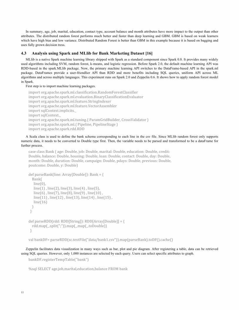
Zeppelin facilitates data visualization in many ways such as bar, plot and pie diagram. After registering a table, data can be retrieved

using SQL queries. However, only 1,000 instances are selected by each query. Users can select specific attributes to graph.

importorg.apache.spark.ml.classification.RandomForestClassifierimportorg.apache.spark.ml.evaluation.BinaryClassificationEvaluatorimportorg.apache.spark.ml.feature.StringIndexerimportorg.apache.spark.ml.feature.VectorAssemblerimportsqlContext.implicits._importsqlContext._importorg.apache.spark.ml.tuning.{ParamGridBuilder,CrossValidator}importorg.apache.spark.ml.{Pipeline,PipelineStage}importorg.apache.spark.rdd.RDD

caseclassBank(age:Double,job:Double,marital:Double,education:Double,credit:Double,balance:Double,housing:Double,loan:Double,contact:Double,day:Double,month:Double,duration:Double,campaign:Double,pdays:Double,previous:Double,poutcome:Double,y:Double)defparseBank(line:Array[Double]):Bank={Bank(line(0),line(1),line(2),line(3),line(4),line(5),line(6),line(7),line(8),line(9),line(10),line(11),line(12),line(13),line(14),line(15),line(16))}defparseRDD(rdd:RDD[String]):RDD[Array[Double]]={rdd.map(_.split(";")).map(_.map(_.toDouble))}valbankDF=parseRDD(sc.textFile("data/bank1.csv")).map(parseBank).toDF().cache()

bankDF.registerTempTable("bank")%sqlSELECTage,job,marital,education,balanceFROMbank

12

Figure 21 Data visualization in Zeppelin

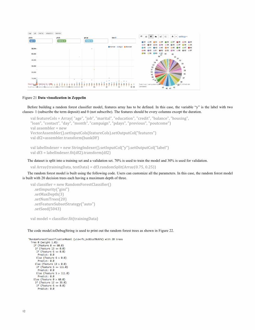
Before building a random forest classifier model, features array has to be defined. In this case, the variable “y” is the label with two classes- 1 (subscribe the term deposit) and 0 (not subscribe). The features should be every columns except the duration.

The dataset is split into a training set and a validation set. 70% is used to train the model and 30% is used for validation.

The random forest model is built using the following code. Users can customize all the parameters. In this case, the random forest model

is built with 20 decision trees each having a maximum depth of three.

The code model.toDebugString is used to print out the random forest trees as shown in Figure 22.

valfeatureCols=Array("age","job","marital","education","credit","balance","housing","loan","contact","day","month","campaign","pdays","previous","poutcome")valassembler=newVectorAssembler().setInputCols(featureCols).setOutputCol("features")valdf2=assembler.transform(bankDF)vallabelIndexer=newStringIndexer().setInputCol("y").setOutputCol("label")valdf3=labelIndexer.fit(df2).transform(df2)

valArray(trainingData,testData)=df3.randomSplit(Array(0.75,0.25))

valclassifier=newRandomForestClassifier().setImpurity("gini").setMaxDepth(3).setNumTrees(20).setFeatureSubsetStrategy("auto").setSeed(5043)valmodel=classifier.fit(trainingData)

13

Figure 22 Random forest visualization

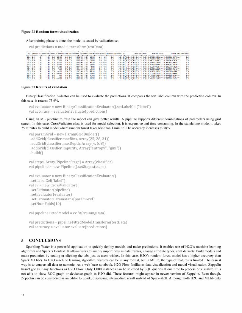
After training phase is done, the model is tested by validation set.

Figure 23 Results of validation

BinaryClassificationEvaluator can be used to evaluate the predictions. It compares the test label column with the prediction column. In this case, it returns 73.6%.

Using an ML pipeline to train the model can give better results. A pipeline supports different combinations of parameters using grid

search. In this case, CrossValidator class is used for model selection. It is expensive and time-consuming. In the standalone mode, it takes 25 minutes to build model where random forest takes less than 1 minute. The accuracy increases to 78%.

5 CONCLUSIONS Sparkling Water is a powerful application to quickly deploy models and make predictions. It enables use of H2O’s machine learning

algorithm and Spark’s Context. It allows users to simply import files as data frames, change attribute types, spilt datasets, build models and make prediction by coding or clicking the tabs just as users wishes. In this case, H2O’s random forest model has a higher accuracy than Spark MLlib’s. In H2O machine learning algorithm, features can be in any format, but in MLlib, the type of features is limited. The easiest way is to convert all data to numeric. As a web-base notebook, H2O Flow facilitates data visualization and model visualization. Zeppelin hasn’t got as many functions as H2O Flow. Only 1,000 instances can be selected by SQL queries at one time to process or visualize. It is not able to show ROC graph or deviance graph as H2O did. These features might appear in newer version of Zeppelin. Even though, Zeppelin can be considered as an editor to Spark, displaying intermediate result instead of Spark-shell. Although both H2O and MLlib only

valpredictions=model.transform(testData)

valevaluator=newBinaryClassificationEvaluator().setLabelCol("label")valaccuracy=evaluator.evaluate(predictions)

valparamGrid=newParamGridBuilder().addGrid(classifier.maxBins,Array(25,28,31)).addGrid(classifier.maxDepth,Array(4,6,8)).addGrid(classifier.impurity,Array("entropy","gini")).build()valsteps:Array[PipelineStage]=Array(classifier)valpipeline=newPipeline().setStages(steps)valevaluator=newBinaryClassificationEvaluator().setLabelCol("label")valcv=newCrossValidator().setEstimator(pipeline).setEvaluator(evaluator).setEstimatorParamMaps(paramGrid).setNumFolds(10)valpipelineFittedModel=cv.fit(trainingData)valpredictions=pipelineFittedModel.transform(testData)valaccuracy=evaluator.evaluate(predictions)

14

contain some popular models, users are allowed to import customized machine learning models or modify configuration parameters. Overall, H2O is a mature and specialized machine learning tool that everyone can get started quickly. Spark MLlib is more suitable for people who have program experience. In this case, the two datasets used for experiments are not large enough to be qualified to “big data”. In the future, I would like to try more examples of “real” big data, and compare the performance of H2O and MLlib.

REFERENCES [1] Zaharia, M., Xin, R. S., Wendell, P., Das, T., Armbrust, M., Dave, A., Meng, X., Rosen, J., Venkataraman, S., Franklin, M. J., Ghodsi, A., Gonzalez, J., Shenker, S., Stoica, I.

2016. Apache Spark: A Unified Engine for Big Data Processing. Communications of the ACM 59, 11, 56–65. DOI:http://dx.doi.org/10.1145/2934664. [2] Meng, X., Bradley, J., Yavuz, B., Sparks, E., Venkataraman, S., Liu, D., Freeman, J., Tsai, D.B., Amde, M., Owen, S. and Xin, D., 2016. Mllib: Machine learning in apache

spark. Journal of Machine Learning Research, 17(34), 1-7. [3] H2O.ai. http://www.h2o.ai [4] Sparkling Water = H20 + Apache Spark. https://databricks.com/blog/2014/06/30/sparkling-water-h20-spark.html [5] The Practical Guide to Machine Learning. http://university.h2o.ai/business-101/downloads/practical-guide-to-machine-learning.pdf [6] DRF — H2O 3.10.0.6 documentation. http://docs.h2o.ai/h2o/latest-stable/h2o-docs/data-science/drf.html [7] GBM — H2O 3.10.0.6 documentation. http://docs.h2o.ai/h2o/latest-stable/h2o-docs/data-science/gbm.html [8] GLM — H2O 3.10.0.6 documentation. http://docs.h2o.ai/h2o/latest-stable/h2o-docs/data-science/glm.html [9] K-Means — H2O 3.10.0.6 documentation. http://docs.h2o.ai/h2o/latest-stable/h2o-docs/data-science/k-means.html [10] Naïve Bayes — H2O 3.10.0.6 documentation. http://docs.h2o.ai/h2o/latest-stable/h2o-docs/data-science/naive-bayes.html [11] PCA — H2O 3.10.0.6 documentation. http://docs.h2o.ai/h2o/latest-stable/h2o-docs/data-science/pca.html [12] Generalized Low Rank Models. http://arxiv.org/abs/1410.0342 [13] Deep Learning. http://www.h2o.ai/verticals/algos/deep-learning/ [14] Apache Zeppelin. https://zeppelin.apache.org/ [15] UCI Machine Learning Repository: default of credit card clients Data Set. https://archive.ics.uci.edu/ml/datasets/default of credit card clients [16] UCI Machine Learning Repository: Bank Marketing Data Set. http://mlr.cs.umass.edu/ml/datasets/Bank+Marketing