DASSO: connections between the Dantzig selector and lasso

© 2009 Royal Statistical Society 1369–7412/09/71127

J. R. Statist. Soc. B (2009)71, Part 1, pp. 127–142

DASSO: connections between the Dantzig selectorand lasso

Gareth M. James, Peter Radchenko and Jinchi Lv

University of Southern California, Los Angeles, USA

[Received September 2007. Revised April 2008]

Summary. We propose a new algorithm, DASSO, for fitting the entire coefficient path of theDantzig selector with a similar computational cost to the least angle regression algorithm thatis used to compute the lasso. DASSO efficiently constructs a piecewise linear path througha sequential simplex-like algorithm, which is remarkably similar to the least angle regressionalgorithm. Comparison of the two algorithms sheds new light on the question of how the lassoand Dantzig selector are related. In addition, we provide theoretical conditions on the designmatrix X under which the lasso and Dantzig selector coefficient estimates will be identical forcertain tuning parameters. As a consequence, in many instances, we can extend the powerfulnon-asymptotic bounds that have been developed for the Dantzig selector to the lasso. Finally,through empirical studies of simulated and real world data sets we show that in practice, whenthe bounds hold for the Dantzig selector, they almost always also hold for the lasso.

Keywords: Dantzig selector; DASSO; Lasso; Least angle regression

1. Introduction

Consider the standard linear regression model,

Y=Xβ+ε, .1/

where Y is an n-vector of responses, X= .x1, x2, . . . , xp/ is an n×p design matrix, β= .β1, . . . ,βp/T is a p-vector of unknown regression coefficients and ε is an n-vector of random errorswith standard deviation σ. An interesting problem in this setting is that of variable selection, i.e.determining which βj �=0. Traditionally, it has generally been assumed that we are dealing withdata where p�n in which case several standard approaches, such as ‘best subset selection’, havebeen proposed. Recently, situations where p is of similar size to n, or even possibly significantlylarger than n, have become increasingly common. Some important examples include functionalregression where the predictor is itself a function, functional magnetic resonance imaging andtomography, gene expression studies where there are many genes and few observations, signalprocessing and curve smoothing. In such situations classical approaches, such as best subsetselection, will generally fail because they are usually not computationally feasible for large p.As a result there has been much development of new variable selection methods that work withlarge values of p. A few examples include the non-negative garrotte (Breiman, 1995), the lasso(Tibshirani, 1996; Chen et al., 1998; Donoho, 2006; Donoho et al., 2006; Bickel et al., 2008;Meinshausen et al., 2007), the adaptive lasso (Zou, 2006), smoothly clipped absolute deviation(Fan and Li, 2001), the elastic net (Zou and Hastie, 2005), least angle regression (the LARS

Address for correspondence: Gareth M. James, Information and Operations Management Department, Uni-versity of Southern California, 401R Bridge Hall, Los Angeles, CA 90089-0809, USA.E-mail: [email protected]

128 G. M. James, P. Radchenko and J. Lv

algorithm) (Efron et al., 2004), adaptive model selection (Shen and Ye, 2002) and the Dantzigselector (Candes and Tao, 2007a,b; Bickel et al., 2008; Meinshausen et al., 2007).

The Dantzig selector has already received a considerable amount of attention. It was designedfor linear regression models such as model (1) where p is large but the set of coefficients is sparse,i.e. most of the βjs are 0. The Dantzig selector estimate β̂ is defined as the solution to

min.‖β̃‖1/ subject to ‖XT.Y−Xβ̃/‖∞�λD, .2/

where ‖·‖1 and ‖·‖∞ respectively represent the L1- and L∞-norms and λD is a tuning parameter.The L1-minimization produces coefficient estimates that are exactly 0 in a similar fashion to thelasso and hence can be used as a variable selection tool. This approach has shown impressiveempirical performance on real world problems involving large values of p. Candes and Tao(2007a) have provided strong theoretical justification for this performance by establishing sharpnon-asymptotic bounds on the L2-error in the estimated coefficients. They showed that the erroris within a factor of log.p/ of the error that would be achieved if the locations of the non-zerocoefficients were known.

For any given λD, the Dantzig selector optimization criterion (2) can be solved fairly efficientlyby using a standard linear programming procedure. However, producing the entire coefficientpath currently requires solving problem (2) over a fine grid of values for λD. This grid approachcan become computationally expensive when, for example, performing cross-validation on largedata sets. By comparison, in their landmark paper Efron et al. (2004) introduced a highly efficientalgorithm called LARS. They demonstrated that the coefficient path of the lasso is piecewiselinear and, with a slight modification, LARS fits the entire lasso path. Note that when we referto LARS in this paper we mean the modified version.

This paper makes two contributions. First, we prove that a LARS-type algorithm can beused to produce the entire coefficient path for the Dantzig selector. Our algorithm, which wecall DASSO for ‘Dantzig selector with sequential optimization’, efficiently constructs a piece-wise linear path through a sequential simplex-like algorithm that identifies the break pointsand solves the corresponding linear programs. DASSO can be thought of as a modification ofLARS, because a small change in one of its steps produces the LARS algorithm. DASSO has asimilar computational cost to that of LARS and produces considerable computational savingsover a grid search. Second, we establish explicit conditions on the design matrix under whichthe Dantzig selector and the lasso will produce identical solutions. We demonstrate empiricallythat at the sparsest points of the coefficient path, where most coefficients are 0, these conditionsusually hold.

As an example, consider the coefficient paths that are plotted in Fig. 1. These plots corres-pond to the diabetes data set that was used in Efron et al. (2004). The data contain 10 baselinepredictors, age, sex, body mass, blood pressure and six blood serum measurements (S1,. . . ,S6),for n= 442 diabetes patients. The response is a measure of progression of disease 1 year afterbaseline. Fig. 1(a) contains the entire set of possible lasso coefficients computed by using theLARS algorithm. Fig. 1(b) illustrates the corresponding coefficients for the Dantzig selectorcomputed by using DASSO. The left-hand sides of each plot represent the sparsest fits wheremost coefficients are 0, and the extreme right-hand sides reflect the ordinary least squares esti-mates. The left 40% of each plot are identical, with the first six variables entering the modelsin the same fashion. However, the fits differ somewhat in the middle portions where S1 entersnext using the lasso whereas S2 enters using the Dantzig selector, before the two fits convergeagain near the ordinary least squares solution. This pattern of identical fits for the sparsestsolutions occurs for every data set that we have examined. Other researchers have noted similarrelationships (Efron et al., 2007). In fact we provide general conditions on the design matrix

DASSO 129

0.0 0.2 0.4 0.6 0.8 1.0

−50

00

500

Standardized L1 Norm(a) (b)

Sta

ndar

dize

d C

oeffi

cien

ts

S1

SE

XA

GE

S4

S2

S5

0.0 0.2 0.4 0.6 0.8 1.0

−50

00

500

Standardized L1 NormS

tand

ardi

zed

Coe

ffici

ents

S1

SE

XA

GE

S4

S2

S5

Fig. 1. (a) Lasso and (b) Dantzig selector coefficient paths on the diabetes data: the regions with standard-ized L1-norms between 0 and 0:4 are identical

X , under which a given lasso solution will be identical to the corresponding Dantzig selectorsolution. This equivalence allows us to apply the impressive non-asymptotic bounds of Candesand Tao (2007a) to the lasso in addition to the Dantzig selector.

The paper is structured as follows. In Section 2 we present our DASSO algorithm and drawconnections to LARS. Both algorithms are demonstrated on three real world data sets. Section 2also provides the theoretical justification for DASSO. General conditions are derived inSection 3 under which the lasso and Dantzig selector solutions will be identical. In particular, weshow that the strong similarities between the two approaches allow us, in many circumstances,to extend the Dantzig selector bounds to the lasso estimates. A detailed simulation study isprovided in Section 4. Finally, we end with a discussion in Section 5. The proofs of all ourresults are provided in Appendix A.

2. DASSO algorithm

In Section 2.1 we present the key elements of our DASSO algorithm. We give the theoreticaljustification for this algorithm in Section 2.2. Using suitable location and scale transformationswe can standardize the predictors and centre the response, so that

n∑

i=1Yi=0,

n∑

i=1Xij=0,

n∑

i=1X2

ij=1, for j=1, . . . , p: .3/

Throughout the paper we assume that conditions (3) hold. However, all numerical results arepresented on the original scale of the data. For a given index set I we shall write XI for thesubmatrix of X consisting of the columns that are indexed by I.

2.1. The algorithmAs with LARS, the DASSO algorithm progresses in piecewise linear steps. At the start of eachstep the variables that are most correlated with the residual vector are identified. These variables


make up the current active set A and together with the current set of non-zero coefficients Bdetermine the optimal direction that the coefficient path should move in. Along this direction,the maximal correlations are reduced towards 0 at the same rate. We then compute the exactdistance that can be travelled before there is a change in either A or B. At this point we adjustthe two sets, and continue. Formally, the algorithm consists of the following steps (to simplifythe notation, we omit superscript ‘l’ whenever possible).

Step 1: initialize β1 as the zero vector in Rp and set l=1.Step 2: let B be the set indexing the non-zero coefficients of βl. Set c=XT.Y−Xβl/, let A bethe active set indexing the covariances in c that are maximal in absolute value and let sA bethe vector containing the signs of those covariances.Step 3: identify either the index to be added to B or the index to be removed from A. Usethe new A and B to calculate the |B|-dimensional direction vector hB= .XT

AXB/−1sA. Let hbe the p-dimensional vector with the components corresponding to B given by hB and theremainder set to 0.Step 4: compute γ, the distance to travel in the direction h until a new covariance enters theactive set or a coefficient path crosses zero. Set βl+1←βl+γh and l← l+1.Step 5: repeat steps 2–4 until ‖c‖∞=0.

The details for steps 3 (‘direction’) and 4 (‘distance’) are provided in Appendix A. As can beseen from the proof of theorem 1 in Section 2.2, the adjustments to A and B in step 3 exactlycorrespond to the changes in the active set and the set of non-zero coefficients of the estimate.Below we discuss the one at a time condition, under which |A|= |B|+ 1 after step 2 and, as aresult, |A|= |B| after step 3. The entire Dantzig selector coefficient path can be constructed bylinearly interpolating β1, β2, . . . , βL, where L denotes the number of steps that the algorithmtakes. Typically, L is of the same order of magnitude as min.n, p/.

Note that both LARS and DASSO start with all the coefficients set to 0 and then add the var-iable that is most correlated with the residual vector. The only difference between the algorithmsis in step 3. In LARS A and B are kept identical, but DASSO chooses B so that the direction.XT

AXB/−1sA produces the greatest reduction in the maximal correlations per unit increase in‖β̂‖1. It turns out that A and B are often identical for DASSO as well, for at least the first fewiterations. Hence, the sparsest sections of the lasso and Dantzig selector coefficient paths areindistinguishable.

To illustrate this point we compared the Dantzig selector and lasso coefficient paths on threereal data sets. The first was the diabetes data that were discussed in Section 1. The second wasa Boston housing data set with p=13 predictors and n=506 observations where the aim wasto predict median house value. The final data set, on intelligence quotient IQ, considered themore difficult situation where p > n. The IQ data contained n= 74 observations and p= 134predictors. The response was a measure of IQ for each individual and the predictors measuredvarious characteristics of the brain as well as gender and race. The coefficient paths for each dataset are plotted in Fig. 2 with full lines for the lasso and broken lines for the Dantzig selector.All three data sets have identical paths at the sparsest solutions, differ to varying degrees inthe middle stages and then converge again at the end. These plots also show that the Dantzigselector paths are less smooth than those for the lasso.

2.2. Theoretical justificationWe have performed numerous comparisons of the DASSO algorithm with the coefficient paththat is produced by using the Dantzig selector applied to a fine grid of λDs. In all cases the

DASSO 131

(a)

(b)

(c)

Fig

.2.

Lass

o(

)an

dD

antz

igse

lect

or(–

––

)co

effic

ient

path

son

thre

edi

ffere

ntda

tase

ts:(

a)di

abet

esda

ta;(

b)B

osto

nho

usin

gda

ta;(

c)IQ

data


results have been identical. Theorem 1 provides a rigorous theoretical justification for the accu-racy of DASSO. As Efron et al. (2004) did for LARS, we assume the following one at a timecondition: along the DASSO path the increases in the active set and the decreases in the set ofnon-zero coefficients happen one at a time. This situation is typical for quantitative data andcan always be realized by adding a little jitter to the response values. Note that both LARS andDASSO can be generalized to cover other scenarios, e.g. the case of several coefficient pathscrossing zero simultaneously. We choose to avoid this generalization, because it would providelittle practical value and detract from the clarity of the presentation.

Theorem 1. If the one at a time condition holds, the DASSO algorithm produces a solution pathfor the Dantzig selector optimization problem (2), with β1 corresponding to λD=‖XTY‖∞and βL corresponding to λD=0.

Theorem 1 can be derived by an inductive argument. The base case is provided by the zerovector β1, which solves optimization problem (2) for all λD at or above the level ‖XTY‖∞. Theinduction step is established in Appendix A. It follows from the proof that |A|=|B|= rank.X/ atthe end of the algorithm. Theorem 1 has an interesting connection with the regularized solutionpaths theory that was developed in Rosset and Zhu (2007). Their results imply that, if the Dantzigselector is viewed as the minimizer of the penalized criterion function ‖XT.Y−Xβ̃/‖∞+ s‖β̃‖1,then the solution path β̂.s/ is piecewise constant. We work with the definition of the Dantzigselector as the solution to the optimization problem (2), and we parameterize the coefficientpaths by λD. Our theorem 1 shows existence of a continuous piecewise linear solution pathβ̂.λD/ with λD=‖XT.Y −X β̂.λD//‖∞.

3. The Dantzig selector versus the lasso

In this section we investigate the relationship between the Dantzig selector and the lasso. Sec-tion 3.1 gives general motivation for the similarities between the two approaches. In Section3.2 formal conditions are provided that guarantee the equivalence of the Dantzig selector andthe lasso. Section 3.3 then uses these conditions to extend the non-asymptotic Dantzig selectorbounds to the lasso.

3.1. ConnectionsAssume that the data are generated from the linear regression model (1). The Dantzig selectorestimate β̂D= β̂D.λD/ is defined as the solution to the Dantzig selector optimization problem(2). The lasso estimate β̂L= β̂L.λL/ is defined by

β̂L=arg minβ̃

. 12‖Y−Xβ̃‖22+λL‖β̃‖1/, .4/

where ‖·‖2 denotes the L2-norm and λL is a non-negative tuning parameter. We can define thelasso estimate equivalently as the solution to

min.‖β̃‖1/ subject to ‖Y−Xβ̃‖22 � s, .5/

for some non-negative s.The Dantzig selector and lasso share some similarities in view of problems (2) and (5). The

only difference is that the Dantzig selector regularizes the sum of absolute coefficients ‖β̃‖1with the L∞-norm of the p-vector XT.Y−Xβ̃/ whereas the lasso regularizes ‖β̃‖1 with theresidual sum of squares. Furthermore, note that vector −2XT.Y−Xβ̃/ is exactly the gradientof the residual sum of squares. As we show in Appendix A, when the tuning parameters λL and

DASSO 133

λD are chosen to be the same, the lasso estimate is always a feasible solution to the Dantzigselector minimization problem, although it may not be an optimal solution. Therefore, whenthe corresponding solutions are not identical, the Dantzig selector solution is sparser, in termsof the L1-norm, than the lasso solution.

These similarities can be made even more striking by noting that the solutions to problems(2) and (5) are respectively equal to those of

min.‖β̃‖1/ subject to ‖XTX.β̃− β̂ls/‖∞� tD .6/

and

min.‖β̃‖1/ subject to ‖X.β̃− β̂ls/‖22 � tL .7/

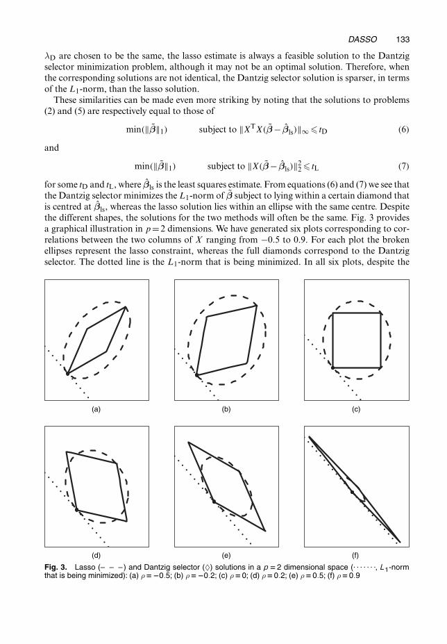
for some tD and tL, where β̂ls is the least squares estimate. From equations (6) and (7) we see thatthe Dantzig selector minimizes the L1-norm of β̃ subject to lying within a certain diamond thatis centred at β̂ls, whereas the lasso solution lies within an ellipse with the same centre. Despitethe different shapes, the solutions for the two methods will often be the same. Fig. 3 providesa graphical illustration in p=2 dimensions. We have generated six plots corresponding to cor-relations between the two columns of X ranging from −0:5 to 0:9. For each plot the brokenellipses represent the lasso constraint, whereas the full diamonds correspond to the Dantzigselector. The dotted line is the L1-norm that is being minimized. In all six plots, despite the

(a) (b) (c)

(d) (e) (f)

Fig. 3. Lasso (– – –) and Dantzig selector (♦) solutions in a p D 2 dimensional space (. . . . . . ., L1-normthat is being minimized): (a) ρD�0:5; (b) ρD�0:2; (c) ρD0; (d) ρD0:2; (e) ρD0:5; (f) ρD0:9


differences in the shapes of the feasible regions, both methods give the same solution, which isrepresented by the larger dot on the L1-line. We show in Section 3.2 that in p=2 dimensions thetwo methods will always be identical, whereas in higher dimensions this will not always be so.In fact, the situation where p� 3 can be different from the case where p= 2, as demonstratedin, for example, Donoho and Tanner (2005), Plumbley (2007) and Meinshausen et al. (2007).

3.2. Conditions for equivalenceDefine IL as the set indexing the non-zero coefficients of β̂L. Let XL be the n× |IL| matrixthat is constructed by taking XIL and multiplying its columns by the signs of the correspondingcoefficients in β̂L. The following result provides easily verifiable sufficient conditions for equalitybetween the Dantzig selector and the lasso solutions.

Theorem 2. Assume that XL has full rank |IL| and λD=λL. Then β̂D= β̂L if

u= .XTLXL/−11�0 and ‖XTXLu‖∞�1, .8/

where 1 is an |IL|-vector of 1s and the vector inequality is understood componentwise.

In theorem 4 in Appendix A we provide a necessary and sufficient condition (14) for the equal-ity of the two solutions, which is in general weaker than the sufficient condition (8). We placedthis theorem in Appendix A because its condition is somewhat difficult to check in practice.The proof of theorem 2 is also given in Appendix A. It should be noted that theorem 2 providesconditions for the lasso and Dantzig solutions to be identical at a given point on the coefficientpath. However, if condition (8) holds for all possible sets |IL|, or even just the sets that aregenerated by the LARS algorithm, then the entire lasso and Dantzig selector coefficient pathswill be identical.

Next we list some special cases where condition (8) will hold at all points of the coefficientpath.

Corollary 1. Assume that X is orthonormal, i.e. XTX= Ip. Then the entire lasso and Dantzigselector coefficient paths are identical.

Corollary 1 holds, because, if X is orthonormal, then XTI XI= I|I| for each index set I. Hence,

condition (8) will hold at all points of the coefficient path. Corollary 1 can be extended to thecase where the columns of X have non-negative correlation, provided that the correlation iscommon among all pairs of columns, which is shown to imply condition (8).

Theorem 3. Suppose that all pairwise correlations between the columns of X are equal to thesame value ρ that lies in [0, 1/. Then the entire lasso and Dantzig selector coefficient paths areidentical. In addition, when p=2, the same holds for each ρ in .−1, 1/.

When p�3 the common correlation ρ cannot be negative because a matrix of this type is nolonger positive definite and thus cannot be a covariance matrix. We stress that in p�3 dimen-sions the equivalence of the Dantzig selector and lasso in general does not hold, and it holds ifand only if condition (14) in Appendix A on the design matrix is satisfied.

We would like to point out that, after the paper was submitted, two recent references, Bickelet al. (2008) and Meinshausen et al. (2007), came to our attention. Bickel et al. (2008) establishedan approximate equivalence between the lasso and Dantzig selector and derived parallel ora-cle inequalities for the prediction risk in the general non-parametric regression model, as wellas bounds on the Lq-estimation loss for 1 � q � 2 in the linear model under assumptions thatare different from ours. Meinshausen et al. (2007) gave a diagonal dominance condition of the

DASSO 135

p×p matrix .XTX/−1 that ensures the equivalence of the lasso and Dantzig selector. Clearly,this diagonal dominance condition implicitly assumes that p � n, whereas our conditions (8)and (14) have no such constraint.

3.3. Non-asymptotic bounds on the lasso errorA major contribution of Candes and Tao (2007a) is establishing oracle properties for the Dant-zig selector under a so-called uniform uncertainty principle (Candes and Tao, 2005) on thedesign matrix X. They proved sharp non-asymptotic bounds on the L2-error in the estimatedcoefficients and showed that the error is within a factor of log.p/ of the error that would beachieved if the locations of the non-zero coefficients were known. These results assume that thetuning parameter is set to the theoretical optimum value of λD=σ

√{2 log.p/}.Recently, there have also been several studies on the lasso with different foci. See, for example,

Meinshausen and Bühlmann (2006), Zhang and Huang (2007) and Zhao and Yu (2006). Someof this work has developed bounds on the lasso error. However, most existing results in this areaare asymptotic. In theorem 2 we identified conditions on the design matrix X under which thelasso estimate is the same as the Dantzig selector estimate. Under these conditions, or undera weaker general condition (14), the powerful theory that has already been developed for theDantzig selector directly applies to the lasso.

4. Simulation study

We performed a series of four simulations to provide comparisons of performance between theDantzig selector and lasso. For each set of simulations we generated 100 data sets and tested sixdifferent approaches. The first involved implementing the Dantzig selector by using the tuningparameter λD that was selected via Monte Carlo simulation as the maximum of |XTZ| over 20realizations of Z∼N.0, σ2I/ as suggested in Candes and Tao (2007a). The second approachused the lasso with the same tuning parameter as that suggested for the Dantzig selector.The next two methods, DS CV and LASSO CV, implemented the Dantzig selector and lassoin each case using the tuning parameter giving the lowest mean-squared error under tenfoldcross-validation. The final two methods, double Dantzig and double lasso, use ideas that wereproposed in James and Radchenko (2008) and Meinshausen (2007). First, the Dantzig selectorand lasso are fitted by using the theoretical optimum. We then discard all parameters with zerocoefficients and refit the Dantzig selector and lasso to the reduced number of predictors withthe tuning parameters chosen by using cross-validation. This two-step approach reduces over-shrinkage of the coefficients. In all cases σ2 was estimated by using the mean sum of squaresfrom the DS CV and LASSO CV methods.

The results for the six approaches applied to the four simulations are summarized in Table 1.Five statistics are provided. The first,

ρ2=

p∑

j=1.β̂j−βj/2

p∑

j=1min.β2

j , σ2/

,

represents the ratio of the squared error between the estimated and true β-coefficients to thetheoretical optimum squared error assuming that the identity of the non-zero coefficients wasknown. The second statistic, pred, provides the mean-squared error in predicting the expected


Table 1. Simulation results measuring accuracy of coefficient estimation ρ2, prediction accuracy pred, num-ber of predictors selected S, false positive rate F C and false negative rate F � for six different methods†

Method Results for simulation 1 Results for simulation 2

ρ2 pred S F+ F− ρ2 pred S F+ F−

Dantzig selector 5.07 0.130 7.08 0.059 0.114 7.42 0.153 7.13 0.058 0.092Lasso 5.07 0.130 7.08 0.059 0.114 7.36 0.152 7.11 0.057 0.090DS CV 3.82 0.099 14.47 0.220 0.082 4.73 0.103 13.96 0.206 0.064LASSO CV 3.81 0.098 13.76 0.204 0.082 4.65 0.101 13.78 0.202 0.064Double Dantzig 2.24 0.060 4.65 0.010 0.160 2.85 0.066 5.08 0.016 0.128Double lasso 2.24 0.060 4.65 0.010 0.160 2.83 0.066 5.08 0.016 0.128

Results for simulation 3 Results for simulation 4

Dantzig selector 6.77 0.141 6.88 0.057 0.138 23.01 2.345 8.86 0.026 0.260Lasso 6.77 0.141 6.89 0.057 0.138 22.42 2.283 9.01 0.027 0.256DS CV 4.57 0.100 15.16 0.236 0.094 9.42 0.969 28.04 0.122 0.142LASSO CV 4.50 0.099 14.18 0.215 0.100 8.82 0.913 24.97 0.106 0.138Double Dantzig 2.98 0.066 4.79 0.014 0.164 8.93 0.917 15.83 0.060 0.164Double lasso 2.99 0.066 4.79 0.014 0.164 9.23 0.947 16.14 0.061 0.168

†Each simulation consisted of 100 different data sets.

response over a large test data set. The next value, S, provides the average number of variablesselected in the final model. The final two statistics, F+ and F−, respectively represent the frac-tion of times that an unrelated predictor is included and the fraction of times that an importantpredictor is excluded from the model.

The first three sets of simulations used data that were generated with n= 200 observationsand p=50 predictors of which only five were related to the response with the true β-coefficientsgenerated from a standard normal distribution. The design matrices X in the first simulationwere generated by using independent and identically distributed (IID) standard normal randomvariables and the error terms were similarly generated from a standard normal distribution. As aresult of the IID entries, the correlations between columns of X were close to 0 (the standarddeviations of the correlations was approximately 0:07). The results of Section 3 suggest that thelasso and Dantzig selector should give similar performance in this setting. This is exactly whatwe observe with the statistics for simulations with the Dantzig selector, DS CV and doubleDantzig almost identical to their lasso counterparts. The Dantzig selector and lasso results arethe worst in terms of coefficient estimation and prediction accuracy. However, both methodsperform well at identifying the correct coefficients (F+ and F− are both low), suggesting over-shrinkage of the true parameters. The cross-validation versions have lower error rates on thecoefficient estimates and predictions but at the expense of including many irrelevant variables.The double Dantzig and double lasso methods provide the best performance, both in terms ofthe coefficients and prediction accuracy and in terms of a low F+-rate with approximately thecorrect number of variables.

The second simulation used data sets with a similar structure to those in the first simulation.However, we introduced significant correlation structure into the design matrix by dividing the50 predictors into five groups of 10 variables. Within each group we randomly generated pre-dictors with common pairwise correlations between 0 and 0:5. Predictors from different groupswere independent. As a result, the standard deviation of the pairwise correlations was twice

DASSO 137

that of the first simulation, which caused a deterioration in most of the statistics. However, allthree versions of the Dantzig selector and lasso still gave extremely similar performance. Addi-tionally, the double Dantzig and double lasso performed best followed by the cross-validatedversions. The third simulation aimed to test the sensitivity of the approaches to the Gaussianerror assumption by repeating the second simulation except that the errors were generated froma Student t-distribution with 3 degrees of freedom. The errors were normalized to have unitstandard deviation. The Dantzig selector and lasso as well as the DS CV and LASSO CV meth-ods actually improved slightly (though the differences were not statistically significant). Thedouble Dantzig and double lasso both showed small deterioration but still outperformed theother approaches.

Finally, the fourth simulation tested out the large p, small n, scenario that the Dantzig selec-tor was originally designed for. We produced design matrices with p=200 variables and n=50observations, using IID standard normal entries. The error terms were also IID standard nor-mal. As with the previous simulations, we used five non-zero coefficients, but their standarddeviation was increased to 2. Not surprisingly, the performance of all methods deteriorated.This was especially noticeable for the Dantzig selector and lasso approaches. Athough thesemethods included roughly the right number of variables, they missed over 25% of the correctvariables and hence had very high error rates. In terms of prediction accuracy, the CV and doubleDantzig or double lasso methods performed similarly. However, as with the other simulations,the CV methods selected far more variables than the other approaches. In this setting the LASSOCV outperformed the DS CV but the double Dantzig outperformed the double lasso method.Both differences were statistically significant at the 5% level. None of the other simulationscontained any statistically significant differences between the lasso and Dantzig selector.

Overall, the simulation results suggest very similar performance between the Dantzig selec-tor and the lasso. To try to understand this result better we computed the differences betweenthe lasso and Dantzig selector paths for each simulation run at each value of λ. For all foursimulations the mean differences in the paths, averaged over all values of λ, were extremely low.The maximum differences were somewhat larger, especially for the fourth simulation. However,among the approaches that we investigated, these differences tended to be in suboptimal partsof the coefficient path. Amazingly, among the 300 data sets in the first three simulations, therewas not a single one where the lasso and Dantzig selector differed when using the theoreticaloptimum value for λ. Even in the fourth simulation, where we might expect significant differ-ences, only about a quarter of the data sets resulted in a difference at the theoretical optimum.This seems to provide strong evidence that the non-asymptotic bounds for the Dantzig selectoralso hold in most situations for the lasso.

5. Discussion

Our aim here has not been definitively to address which approach is superior: the lasso orDantzig selector. Rather, we identify the similarities between the two methods and, throughour simulation study, provide some suggestions about the situations where one approach mayoutperform the other.

Our DASSO algorithm means that the Dantzig selector can be implemented with similarcomputational cost to that of the lasso. Modulo one extra calculation in the direction step,the LARS and DASSO algorithms should perform equally fast. As a result of its optimizationcriterion, for the same value of ‖β̂‖1 the Dantzig selector does a superior job of driving thecorrelation between the predictors and the residual vector to 0. In searching for these reducedcorrelations the Dantzig selector tends to produce less smooth coefficient paths: a potential


concern if the coefficient estimates change dramatically for a small change in λD. Our simu-lation results suggest that in practice the rougher paths may cause a small deterioration inaccuracy when using cross-validation to choose the tuning parameter. However, averaged overall four simulations, the performance of the double Dantzig method was the best of the sixapproaches that we examined, suggesting that this method may warrant further investigation.Finally, it is worth mentioning that, although our focus here has been on linear regression, theDASSO algorithm can also be used in fields such as compressive sensing (Baraniuk et al., 2008;Candes et al., 2006), where the Dantzig selector is frequently applied to recover sparse signalsfrom random projections.

Acknowledgements

We thank the Associate Editor and referees for many helpful suggestions that improved the pa-per. The IQ data set was kindly supplied by Dr Adrian Raine. This work was partially supportedby National Science Foundation grant DMS-0705312. Lv’s research was partially supported byNational Science Foundation grant DMS-0806030 and the 2008 Zumberge Individual Awardfrom the James H. Zumberge Faculty Research and Innovation Fund at the University of South-ern California.

Appendix A: Direction step

Write β+ and β− for the positive and negative parts of βl. Suppose that the indices in A are orderedaccording to the time that they were added and write SA for the diagonal matrix whose diagonal is givenby sA. The set-up of the algorithm and the one at a time condition ensure that |A|= |B|+1. If the set B isempty, add to it the index of the variable that is most correlated with the current residual. In all other cases,the index to be either added to B or removed from A is determined by the calculations in the followingthree steps.

Step 1: compute the |A |× 2p+|A|matrix A= .−SAXTAX SAXT

AX I/, where I is the identity matrix.The first p columns correspond to β+ and the next p columns to β−.Step 2: let B̃ be the matrix that is produced by selecting all the columns of A that correspond to thenon-zero components of β+ and β−, and let Ai be the ith column of A. Write B̃ and Ai in the followingblock form:

B̃=(

B1

B2

),

Ai=(

Ai1

Ai2

),

where B1 is a square matrix of dimension |A|−1, and Ai2 is a scalar. Define

iÅ= arg maxi:qi �=0,α=qi>0

.1TB−11 Ai1 −1{i�2p}/|qi|−1 .9/

where qi=Ai2 −B2B−11 Ai1 and α=B2B

−11 1−1.

Step 3: if iÅ �2p, augment B by the index of the corresponding β-coefficient. If iÅ=2p+m for m�1,leave B unchanged, but remove the mth element from the set A.

Note that B−11 is typically the .XT

AXB/−1 matrix from the previous iteration of the algorithm. In addition,the current .XT

AXB/−1 matrix can be efficiently computed by using a simple update from B−11 , as can be

seen from the proof of lemma 1 in Appendix C.1.

Appendix B: Distance step

The following formulae for computing the distance until the next break point on the coefficient path areexactly the same as those for the LARS algorithm. There are two scenarios that can cause the coefficientpath to change direction. The first occurs when

DASSO 139

maxj∈Ac|xT

j {Y−X.βl+γh/}|=maxj∈A|xT

j {Y−X.βl+γh/}|,because this is the point where a new variable enters the active set A. Standard algebra shows that the firstpoint at which this will happen is given by

γ1=+

minj∈Ac

{ck− cj

.xk−xj/TXh,

ck+ cj

.xk+xj/TXh

},

where min+ is the minimum taken over the positive components only, ck and cj are the kth and jth com-ponents of c evaluated at βl and xk represents any variable that is a member of the current active set.The second possible break in the path occurs if a coefficient path crosses zero, i.e. βl

j+γhj=0. It is easilyverified that the corresponding distance is given by γ2=min+j {−βl

j=hj}. Combining the two possibilities,we set γ=min{γ1, γ2}.

Appendix C: Proof of theorem 1

As we have mentioned, β1 solves the Dantzig selector optimization problem (2) for λD=‖XTY‖∞. Weneed to establish the induction step between βl and βl+1 for l < L. Throughout this section we assumethat the one at a time condition holds, A, B and c are defined as in step 2 of the DASSO algorithm andh is defined as in step 3 of the algorithm. Suppose that we have established that βl solves problem (2) forλD=‖c‖∞. It is left to show that βl+ th solves problem (2) for λD=‖c‖∞− t and t in [0, γ]. This fact is aconsequence of the following result, which we prove at the end of the section.

Lemma 1. For each t in [0, γ], vector βl.t/=βl+ th solves the optimization problem

min.‖β̃‖1/ subject to SAXTA.Y−Xβ̃/�‖c‖∞− t: .10/

Optimization problems (2) and (10) have the same criterion, but the constraint set in problem (2) is asubset of the constraint set in problem (10). Hence, if βl.t/ is a feasible solution for problem (2), it is alsoan optimal solution. The Dantzig selector constraints that remain active throughout the current iterationof the algorithm are satisfied for βl.t/, because the corresponding covariances do not change their signs inbetween the two break points. The remaining constraints are automatically satisfied because of the choiceof γ in the distance step of the algorithm. This completes the proof of theorem 1.

C.1. Proof of lemma 1For concreteness assume that the lth break point occurred because of an increase in the active set A. Theproof for the zero-crossing case is almost identical. Denote the size of A by K and recall the definitionsfrom appendices A and B. Note that the K columns of X given by A are linearly independent because, fora column to enter the active set, it must be linearly independent from the columns that are already in it.Consequently, rank.A/=K. Let d stand for the .2p+K/-vector with 1s for the first 2p components and0s for the remaining components, and write b for the K -vector .‖c‖∞ − t/1−SAXT

AY. Problem (10) canbe reformulated as a linear program:

min.dTx/ subject to Ax=b, x �0: .11/

The correspondence between vectors x and β̃ is as follows: the first p components of x contain the positiveparts of β̃, the second p components of x contain the negative parts and the remaining K componentsare slack variables that correspond to the K constraints in optimization problem (10). Write xl for thevector corresponding to βl and let x̃l stand for the subvector of non-zero elements of xl with one extra 0at the bottom. Note that xl has K−1 non-zero components, but the number of active constraints has justincreased to K ; hence we must increase the number of non-zero components to satisfy the constraints.

We shall search for an optimal solution to the linear program (11) among those vectors that have exactlyK non-zero components. Write B for a K×K submatrix of A whose first K−1 columns correspond to theK− 1 non-zero components of xl. We shall consider solutions whose non-zero components correspondto the columns of B. Each feasible solution of this form is represented by the subvector xB of length Kthat satisfies xB=B−1b. Such B is necessarily invertible, because otherwise its last column is just a linearcombination of the rest; thus continuing the solution path through the lth break point along the originaldirection would not violate the constraints, which is impossible. The following fact is established by stand-


ard linear programming arguments; for example see page 298 of Bazaraa et al. (1990). The last column ofB can be assigned in such a way that, if we define xB.t/= x̃l− tB−11 and let δ be the first positive t at whicha component of xB.t/ crosses zero, then vector xB.t/ represents an optimal solution to the linear program(11) for each t in [0, δ]. We shall now check that the index of the correct last column to be assigned to B isthe index that is specified by equation (9) in the direction step of the algorithm.

Suppose that we try Ai as the last column of matrix B. Simple algebra shows that B is invertible if andonly if qi �=0, and the inverse has the following four-block form:

B−1=(

B−11 +B−1

1 Ai1 B2B−11 q−1

i −B−11 Ai1 q−1

i

−B2B−11 q−1

i q−1i

): .12/

Observe that when an Ai corresponding to a β+j is replaced by the column corresponding to β−j , or viceversa, the sign of α=qi is flipped; hence the set {i : qi �= 0, α=qi � 0} is non-empty. Write dB for the sub-vector of d corresponding to the columns of B. The cost value that is associated with xB.t/ is given bydT

BB−1b=dTxl− tdTBB−11. Formula (12) implies that

dTBB−11=1TB−1

1 1+ .1TB−11 Ai1 −1{i�2p}/α=qi: .13/

For each t in [0, δ], the last component of xB.t/ has the same sign as the last component of −B−11, whichis given by α=qi. Thus, xB.t/ is a feasible solution if and only if α=qi �0. Note that α=0 would imply thatthe first K−1 components of B−11 are given by B−1

1 1, which again leads to a contradiction. Consequently,using AiÅ as the last column of B will produce an optimal solution if and only if iÅ maximizes the secondterm on the right-hand side of equation (13) over the set {i : qi �=0, α=qi > 0}, as is prescribed, indeed, bythe direction step. Because γ � δ by the definition of γ in the distance step, βl+ th is an optimal solutionto problem (10) for each t in [0, γ].

Appendix D: Proof of theorem 2

Define two index sets, I1= {1 � j � p : ζj =λL} and I2= {1 � j � p : ζj =−λL}, where XT.Y−Xβ̂L/=.ζ1, . . . , ζp/T, and let I = I1 ∪ I2. For notational convenience, we let f.β̃/= ‖β̃‖1. Let XI1,I2 be ann× |I| matrix that is generated from the columns of X that correspond to the indices in I after multi-plying those columns in index set I2 by −1. Define two index sets I0

1 = I1 ∩ IL and I02 = I2 ∩ IL: We show

in the proof of theorem 4 that IL⊂ I= I1 ∪ I2, and thus it follows that I01 ∪ I0

2 = IL. Define matrix XI01 ,I0

2analogously to XI1,I2 . Note that XI01 ,I0

2and XL are identical. Hence, it is easy to see that, provided that

I= IL, condition (14) holds whenever condition (8) is true. By setting certain elements of u to 0 the sameresult also holds at the break points where IL is a subset of I. Therefore, theorem 2 is a direct consequenceof the following result.

Theorem 4. Assume that XTXI1,I2 has full rank |I| and λD=λL. Then β̂D= β̂L if and only if there is an|I|-vector u with non-negative components such that

0∈ @β̃f.β̂L/−XTXI1,I2 u, .14/

where @β̃f.β̂L/={.v1, . . . , vp/T : vj= sgn.β̂L, j/ if j∈ IL and vj ∈ [−1, 1] otherwise}.

We spend the remainder of this section proving theorem 4. Denote by l.β̃, λL/ the objective func-tion in equation (4). It is easy to see that l.β̃, λL/ is a convex function in β̃, and thus the zero p-vector 0belongs to the subdifferential @β̃l.β̂L, λL/ since β̂L minimizes l.β̃, λL/. The subdifferential of l.β̃, λL/ in β̃ isgiven by

@β̃l.β̃, λL/= 12∇β̃‖Y−Xβ̃‖2

2+λL@β̃‖β̃‖1

=−XT.Y−Xβ̃/+λL@β̃‖β̃‖1,

where it is a known fact that, for β̃= .β1, . . . , βp/T,

@β̃‖β̃‖1={v= .v1, . . . , vp/T : vj= sgn.βj/ if βj �=0 and vj ∈ [−1, 1] if βj=0, i=1, . . . , p}:

Thus, there is some v∈@β̃‖β̃‖1 at β̂L such that XT.Y−Xβ̂L/−λLv=0. In particular, we see that ‖XT.Y−Xβ̂L/‖∞�λL. Note that the set of indices IL={1� j �p : β̂L,j �=0} that is selected by the lasso is a subset

DASSO 141

of the index set I = {1 � j � p : |ζj| = λL} and, for any j ∈ IL, ζj = sgn.β̂L,j/λL, where .ζ1, . . . , ζp/T =XT.Y−Xβ̂L/.

Now take λD=λL. Then, we have shown that β̂L is a feasible solution to the minimization problem(2), but it might not be an optimal solution. Let us investigate when β̂L is indeed the Dantzig selector, i.e.a solution to problem (2). We make a simple observation that the constraint ‖XT.Y−Xβ̃/‖∞�λD canequivalently be written into a set of 2p linear constraints, xT

j .Y−Xβ̃/ � λD and −xTj .Y−Xβ̃/ � λD,

j=1, . . . , p.Suppose that the p× |I| matrix XTXI1,I2 has full rank |I|, which means that all its column p-vectors

are linearly independent. Clearly, this requires that |I|� min.n, p/. Since the minimization problem (2)is convex, it follows from classical optimization theory that β̂L is a solution to problem (2) if and only ifit is a Karush–Kuhn–Tucker point, i.e. there is an |I|-vector u with non-negative components such that0∈@β̃f.β̂L/−XTXI1,I2 u, where the matrix XTXI1,I2 is associated with the gradients of the linear constraintsin the Dantzig selector.

Appendix E: Proof of theorem 3

When all the column n-vectors of the n×p design matrix X have unit norm and equal pairwise correlationρ it will be the case that

XTX=A= .1−ρ/Ip+ρ11T: .15/

A direct calculation using the Sherman–Morrison–Woodbury formula gives

A−1= 11−ρ

Ip− ρ

.1−ρ/{1+ .p−1/ρ}11T, .16/

which shows that A is invertible for each ρ∈ [0, 1/. Thus, equation (15) in fact entails that p�n.Now, we show that equation (15) implies condition (8). Note that all principal submatrices of A have

the same form as A. Thus, to show that the first part of condition (8) holds, without loss of generality weneed only to show that it holds for IL= {1, . . . , p}. Let v= .v1, . . . , vp/T be a p-vector with components1 or −1, where {1 � j �p : vj = 1}= I0

1 and {1 � j �p : vj =−1}= I02 . It follows from equation (15) that

u= .XLXL/−11= diag.v/A−1v, where diag(v) denotes a diagonal matrix with diagonal elements being thecomponents of vector v. Then, we need to prove that diag.v/A−1v �0. Note that diag.v/v=1, diag.v/1= vand |1Tv|�p. Thus, by equation (16), we have, for any ρ∈ [0, 1/,

diag.v/A−1v= 11−ρ

(1− 1Tvρ

1−ρ+pρv)

�0,

which proves the first part of condition (8).It remains to prove the second part of condition (8). We need only to show that, for each j∈{1, . . . , p}\IL,

|xTj XLu|�1: .17/

Let v be an |IL|-vector with components 1 or −1, where {1� j � |IL| : vj=1} and {1� j � |IL| : vj=−1}correspond to I0

1 and I02 in the index set IL respectively. We denote by Ap=A to emphasize its order. Then,

we have shown that

u= .XTLXL/−11=diag.v/A−1

|IL |v=1

1−ρ

(1− 1Tvρ

1−ρ+|IL|ρ v)

�0: .18/

Note that all the off-diagonal elements of A are ρ. Hence it follows from equation (18), equality vTv=|IL|and inequality |vT1|� |IL| that, for each ρ∈ [0, 1/,

|xTj XLu|= |ρvTu|=

∣∣∣∣ ρ

1−ρ

(1− 1Tvρ

1−ρ+|IL|ρ v)∣∣∣∣

=∣∣∣∣ ρ

1−ρvT1

(1− |IL|ρ

1−ρ+|IL|ρ)∣∣∣∣� |IL|ρ

1−ρ

1−ρ

1−ρ+|IL|ρ= |IL|ρ

1−ρ+|IL|ρ < 1,

which proves inequality (17).


References

Baraniuk, R., Davenport, M., DeVore, R. and Wakin, M. (2008) A simple proof of the restricted isometry propertyfor random matrices. Construct. Approximn, to be published.

Bazaraa, M., Jarvis, J. and Sherali, H. (1990) Linear Programming and Network Flows, 2nd edn. New York: Wiley.Bickel, P. J., Ritov, Y. and Tsybakov, A. (2008) Simultaneous analysis of Lasso and Dantzig selector. Ann. Statist.,

to be published.Breiman, L. (1995) Better subset regression using the non-negative garrote. Technometrics, 37, 373–384.Candes, E. and Romberg, J. (2006) Quantitative robust uncertainty principles and optimally sparse decomposi-

tions. Foundns Comput. Math., 6, 227–254.Candes, E., Romberg, J. and Tao, T. (2006) Robust uncertainty principles: exact signal reconstruction from highly

incomplete frequency information. IEEE Trans. Inform. Theory, 52, 489–509.Candes, E. and Tao, T. (2005) Decoding by linear programming. IEEE Trans. Inform. Theory, 51, 4203–4215.Candes, E. and Tao, T. (2007a) The Dantzig selector: statistical estimation when p is much larger than n. Ann.

Statist., 35, 2313–2351.Candes, E. and Tao, T. (2007b) Rejoinder—the Dantzig selector: Statistical estimation when p is much larger

than n. Ann. Statist., 35, 2392–2404.Chen, S., Donoho, D. and Saunders, M. (1998) Atomic decomposition by basis pursuit. SIAM J. Scient. Comput.,

20, 33–61.Donoho, D. (2006) For most large underdetermined systems of linear equations, the minimal l1-norm near-solu-

tion approximates the sparsest near-solution. Communs Pure Appl. Math., 59, 907–934.Donoho, D., Elad, M. and Temlyakov, V. (2006) Stable recovery of sparse overcomplete representations in the

presence of noise. IEEE Trans. Inform. Theory, 52, 6–18.Donoho, D. and Tanner, J. (2005) Sparse nonnegative solution of underdetermined linear equations by linear

programming. Proc. Natn. Acad. Sci. USA, 102, 9446–9451.Efron, B., Hastie, T., Johnstone, I. and Tibshirani, R. (2004) Least angle regression (with discussion). Ann. Statist.,

32, 407–451.Efron, B., Hastie, T. and Tibshirani, R. (2007) Discussion of the “dantzig selector”. Ann. Statist., 35, 2358–2364.Fan, J. and Li, R. (2001) Variable selection via nonconcave penalized likelihood and its oracle properties. J. Am.

Statist. Ass., 96, 1348–1360.James, G. M. and Radchenko, P. (2008) A generalized Dantzig selector with shrinkage tuning. Technical Report.

University of Southern California, Los Angeles.Meinshausen, N. (2007) Relaxed Lasso. Computnl Statist. Data Anal., 52, 374–393.Meinshausen, N. and Bühlmann, P. (2006) High dimensional graphs and variable selection with the lasso. Ann.

Statist., 34, 1436–1462.Meinshausen, N., Rocha, G. and Yu, B. (2007) A tale of three cousins: Lasso, L2Boosting, and Dantzig (discussion

on Candes and Tao’s Dantzig Selector paper). Ann. Statist., 35, 2372–2384.Plumbley, M. D. (2007) On polar polytopes and the recovery of sparse representations. IEEE Trans. Inform.

Theory, 53, 3188–3195.Rosset, S. and Zhu, J. (2007) Piecewise linear regularized solution paths. Ann. Statist., 35, 1012–1030.Shen, X. and Ye, J. (2002) Adaptive model selection. J. Am. Statist. Ass., 97, 210–221.Tibshirani, R. (1996) Regression shrinkage and selection via the lasso. J. R. Statist. Soc. B, 58, 267–288.Zhang, C.-H. and Huang, J. (2007) Model-selection consistency of the lasso in high-dimensional linear regression.

Manuscript.Zhao, P. and Yu, B. (2006) On model selection consistency of lasso. J. Mach. Learn. Res., 7, 2541–2563.Zou, H. (2006) The adaptive lasso and its oracle properties. J. Am. Statist. Ass., 101, 1418–1429.Zou, H. and Hastie, T. (2005) Regularization and variable selection via the elastic net. J. R. Statist. Soc. B, 67,

301–320.

DASSO: connections between the Dantzig selector and lasso

Documents

Transcript of DASSO: connections between the Dantzig selector and lasso