
Darryl McLeod, Overview Lecture 5 Economic Growth...
47
Empirical evidence of convergence among nations & people Darryl McLeod, Overview Lecture 5 Economic Growth & Development Econ 6470 Spring 2014
Transcript of Darryl McLeod, Overview Lecture 5 Economic Growth...

Empirical evidence of convergence among nations &
people
Darryl McLeod, Overview Lecture 5
Economic Growth & Development
Econ 6470 Spring 2014

The reality of convergence is important for people and nations (and sustainable development)
• Inequality among nations has increased, but inequality among people has decreased.
• Many nations are catching up with the U.S. see chapter 4 of Eclipse and
• Openness has played a role…. China, Asia, RER
• Convergence in health, education and longevity faster than incomes (or is happening despite diverging incomes) see HDR 2010

The reality of convergence is very important in growth theory
• Endogenous growth driven by savings or R&D need not lead to absolute convergence…
• Absolute convergence is implied by diminishing returns, in the SS model for example,
• Openness should accelerate convergence… this is why Sachs & Warner so warmly received…
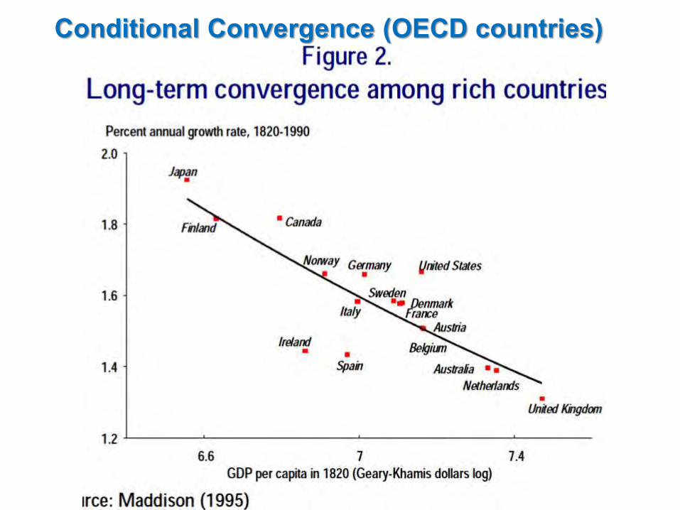
• Conditional convergence is key empirical result of new growth literature

Absolute convergence rare: for example Jones Appendix C data Set: growth 60-97 not related to Y60
-.02
-.01
.00
.01
.02
.03
.04
.05
.06
.07
0.0 0.2 0.4 0.6 0.8 1.0
Y60
G60
97
Dependent Variable: G6097Method: Least SquaresDate: 03/20/13 Time: 17:58Sample: 1 109Included observations: 109White heteroskedasticity-consistent standard errors & covariance
Variable Coefficien... Std. Error t-Statistic Prob.
C 0.017540 0.002330 7.527275 0.0000Y60 0.001675 0.005041 0.332308 0.7403
R-squared 0.000592 Mean dependent var 0.017925Adjusted R-squared -0.008748 S.D. dependent var 0.015765S.E. of regression 0.015834 Akaike info criterion -5.435152Sum squared resid 0.026826 Schwarz criterion -5.385769Log likelihood 298.2158 Hannan-Quinn criter. -5.415125F-statistic 0.063381 Durbin-Watson stat 1.135123Prob(F-statistic) 0.801713 Wald F-statistic 0.110429Prob(Wald F-statistic... 0.740307
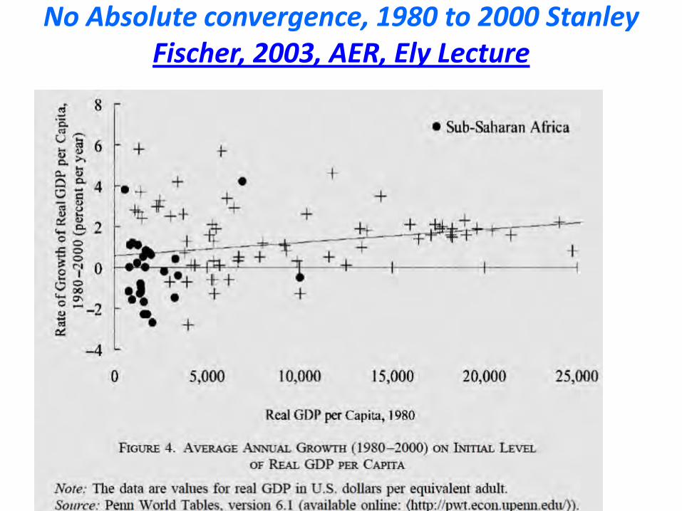
No Absolute convergence, 1980 to 2000 Stanley Fischer, 2003, AER, Ely Lecture

Conditional convergence works just add education for example (Resid is growth not explained by education)
Dependent Variable: G6097Method: Least SquaresDate: 03/20/13 Time: 18:06Sample: 1 109Included observations: 88White heteroskedasticity-consistent standard errors & covariance
Variable Coefficien... Std. Error t-Statistic Prob.
C -0.001137 0.002684 -0.423575 0.6729Y60 -0.053182 0.007145 -7.443537 0.0000
SCHOOL95 0.005650 0.000627 9.012843 0.0000
R-squared 0.441698 Mean dependent var 0.019163Adjusted R-squared 0.428561 S.D. dependent var 0.015126S.E. of regression 0.011435 Akaike info criterion -6.070845Sum squared resid 0.011114 Schwarz criterion -5.986391Log likelihood 270.1172 Hannan-Quinn criter. -6.036821F-statistic 33.62362 Durbin-Watson stat 1.927451Prob(F-statistic) 0.000000 Wald F-statistic 40.63922Prob(Wald F-statistic... 0.000000
-.04
-.03
-.02
-.01
.00
.01
.02
.03
.04
0.0 0.2 0.4 0.6 0.8 1.0
Y60
RE
SID

But we do find absolute convergence, 2000 to 2013,
all IMF WEO countries with >2 million population
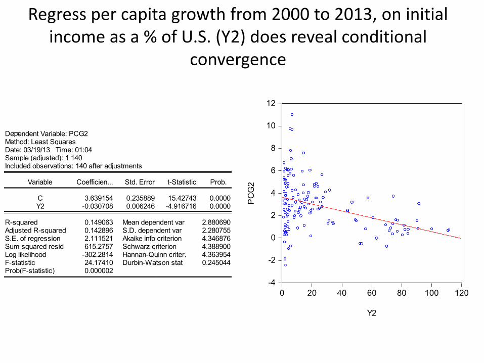
Regress per capita growth from 2000 to 2013, on initial income as a % of U.S. (Y2) does reveal conditional
convergence
Dependent Variable: PCG2Method: Least SquaresDate: 03/19/13 Time: 01:04Sample (adjusted): 1 140Included observations: 140 after adjustments
Variable Coefficien... Std. Error t-Statistic Prob.
C 3.639154 0.235889 15.42743 0.0000Y2 -0.030708 0.006246 -4.916716 0.0000
R-squared 0.149063 Mean dependent var 2.880690Adjusted R-squared 0.142896 S.D. dependent var 2.280755S.E. of regression 2.111521 Akaike info criterion 4.346876Sum squared resid 615.2757 Schwarz criterion 4.388900Log likelihood -302.2814 Hannan-Quinn criter. 4.363954F-statistic 24.17410 Durbin-Watson stat 0.245044Prob(F-statistic) 0.000002
-4
-2
0
2
4
6
8
10
12
0 20 40 60 80 100 120
Y2
PC
G2

Stanley Fischer, 2003, AER, Ely Lecture

Absolute convergence, 2000 to 2013, large countries,
at either end, people’s incomes converging as well

% of U.S. Line Avg per capita growth 2000 to 2013 Pop
1 0.6 3.6 3.3 -0.3 DR Congo 77
2 1.2 3.6 1.8 -1.8 Burundi 9.0
3 1.3 3.6 6.7 3.1 Myanmar 65
4 1.3 3.6 5.4 1.8 Mozambique 23
5 1.3 3.6 5.9 2.3 Ethiopia 91
6 1.4 3.6 2.5 -1.1 Niger 16
7 1.4 3.6 0.3 -3.3 Liberia 4.1
8 1.4 3.6 4.1 0.5 Sierra Leone 6.3
9 1.6 3.6 3.0 -0.6 Malawi 17
10 1.6 3.6 5.2 1.6 Rwanda 11
11 1.8 3.6 -0.4 -3.9 Central African Republic 5.0
12 1.9 3.6 0.6 -3.0 Mali 17
13 2.1 3.6 -1.9 -5.5 Eritrea 5.8
14 2.2 3.6 0.9 -2.7 Madagascar 23
15 2.2 3.6 3.5 -0.1 Uganda 37
16 2.2 3.6 4.8 1.2 Tanzania 44
17 2.2 3.6 1.2 -2.4 Togo 6.4
18 2.2 3.6 2.2 -1.3 Nepal 32
19 2.3 3.6 3.0 -0.5 Burkina Faso 18
20 2.5 3.6 0.5 -3.0 Guinea 11
21 2.5 3.6 -2.4 -6.0 Zimbabwe 13
22 2.5 3.6 5.2 1.6 Tajikistan 8.1
23 2.5 3.6 3.8 0.2 Chad 11
24 2.6 3.6 6.2 2.6 Cambodia 15
25 2.6 3.6 3.8 0.2 Zambia 14
26 2.6 3.6 4.9 1.3 Bangladesh 152
27 2.6 3.6 0.5 -3.1 Guinea-Bissau 1.8
28 2.8 3.6 3.9 0.4 Lesotho 2.0
29 3.0 3.5 0.3 -3.3 Haiti 10
30 3.2 3.5 4.5 1.0 Nigeria 169
Rank
2000
Table C-2: A number of poorest countries grow rapidlyRank 2000% of U.S. Line Avg per capita growth 2000 to 2013 Pop
110 44 2.3 2.5 0.2 Oman 3.3
111 47 2.2 3.2 1.0 Korea 50
112 49 2.1 1.6 -0.5 Saudi Arabia 29
113 50 2.1 1.5 -0.6 Slovenia 2.0
114 52 2.0 -0.5 -2.5 Portugal 11
115 53 2.0 -0.5 -2.5 Greece 11
116 56 1.9 0.8 -1.1 New Zealand 4.5
117 58 1.9 3.6 1.7 Taiwan Province of China 24
118 61 1.8 1.8 0.0 Israel 7.9
119 63 1.7 0.0 -1.7 Spain 46
120 69 1.5 1.2 -0.4 Finland 5.5
121 70 1.5 -0.7 -2.2 Italy 61
122 72 1.4 0.6 -0.8 United Kingdom 63
123 73 1.4 0.9 -0.5 Japan 127
124 74 1.4 0.4 -1.0 France 64
125 74 1.4 1.3 -0.1 Germany 82
126 74 1.4 3.7 2.4 Hong Kong SAR 7.2
127 76 1.3 1.6 0.3 Sweden 9.5
128 77 1.3 0.6 -0.7 Belgium 11
129 77 1.3 1.6 0.3 Australia 23
130 81 1.2 0.3 -0.9 Denmark 5.6
131 82 1.1 1.1 0.0 Austria 8.5
132 82 1.1 0.7 -0.4 Canada 35
133 84 1.1 0.4 -0.6 Ireland 4.5
134 84 1.0 0.8 -0.3 Netherlands 17
135 90 0.9 1.5 0.7 Kuwait 3.9
136 91 0.8 0.9 0.0 Switzerland 8.1
137 92 0.8 3.1 2.2 Singapore 5.5
138 100 0.6 0.8 0.2 United States 317
139 111 0.2 0.6 0.4 Norway 5.1
140 112 0.2 0.7 0.5 United Arab Emirates 5.7
Table C-2 (cont.): OECD country growth slows
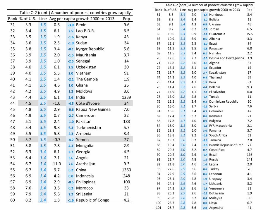
Rank 2000% of U.S. Line Avg per capita growth 2000 to 2013 Pop
31 3.3 3.5 0.6 -3.0 Benin 9.6
32 3.4 3.5 6.1 2.5 Lao P.D.R. 6.5
33 3.5 3.5 1.9 -1.6 Kenya 43
34 3.6 3.5 2.5 -1.0 Sudan 34
35 3.8 3.5 3.4 -0.1 Kyrgyz Republic 5.6
36 3.9 3.5 2.0 -1.5 Mauritania 3.7
37 3.9 3.5 1.0 -2.5 Senegal 14
38 4.0 3.5 6.1 2.5 Uzbekistan 30
39 4.0 3.5 5.5 2.0 Vietnam 91
40 4.1 3.5 1.4 -2.1 The Gambia 1.9
41 4.1 3.5 4.6 1.0 Ghana 26
42 4.2 3.5 4.9 1.3 Moldova 3.6
43 4.4 3.5 6.1 2.6 India 1239
44 4.5 3.5 -1.0 -4.5 Côte d'Ivoire 24
45 4.8 3.5 2.9 -0.6 Papua New Guinea 7.0
46 4.9 3.5 0.7 -2.7 Cameroon 22
47 5.1 3.5 2.4 -1.0 Pakistan 183
48 5.4 3.5 9.8 6.3 Turkmenistan 5.7
49 5.5 3.5 5.8 2.3 Armenia 3.4
50 5.7 3.5 -0.7 -4.2 Yemen 27
51 5.8 3.5 7.8 4.3 Mongolia 2.9
52 6.3 3.4 6.1 2.7 Georgia 4.5
53 6.4 3.4 7.1 3.6 Angola 21
54 6.7 3.4 11.0 7.6 Azerbaijan 9.3
55 6.7 3.4 9.7 6.2 China 1360
56 6.9 3.4 4.2 0.8 Indonesia 248
57 6.9 3.4 2.9 -0.5 Philippines 100
58 7.6 3.4 3.6 0.2 Morocco 33
59 7.9 3.4 5.6 2.2 Sri Lanka 21
60 8.2 3.4 1.8 -1.6 Republic of Congo 4.2
Table C-2 (cont.) A number of poorest countries grow rapidlyRank 2000% of U.S. Line Avg per capita growth 2000 to 2013 Pop
61 8.5 3.4 2.0 -1.4 Honduras 8.4
62 8.8 3.4 2.4 -1.0 Bolivia 11
63 9.1 3.4 4.3 0.9 Ukraine 45
64 9.2 3.4 3.2 -0.2 Jordan 6.5
65 10.6 3.3 0.9 -2.4 Guatemala 15.5
66 10.9 3.3 3.9 0.6 Albania 3.3
67 11.1 3.3 2.3 -1.0 Egypt 84
68 11.5 3.3 2.5 -0.8 Paraguay 6.8
69 11.5 3.3 3.4 0.1 Namibia 2.2
70 12.6 3.3 2.7 -0.5 Bosnia and Herzegovina 3.9
71 12.8 3.2 2.0 -1.3 Algeria 37
72 13.4 3.2 3.1 -0.1 Ecuador 15
73 13.7 3.2 6.0 2.7 Kazakhstan 17
74 14.2 3.2 4.0 0.8 Thailand 65
75 14.4 3.2 4.7 1.5 Peru 31
76 14.4 3.2 7.6 4.4 Belarus 9.3
77 14.9 3.2 1.1 -2.1 El Salvador 6.0
78 15.0 3.2 2.8 -0.4 Tunisia 11
79 15.2 3.2 3.4 0.3 Dominican Republic 10
80 16.0 3.1 2.7 -0.5 Serbia 7.6
81 16.6 3.1 3.4 0.3 Colombia 47
82 17.4 3.1 3.7 0.6 Romania 21
83 17.8 3.1 4.0 0.9 Bulgaria 7.2
84 18.0 3.1 3.0 -0.1 FYR Macedonia 2.1
85 18.8 3.1 6.0 3.0 Panama 3.7
86 18.8 3.1 2.2 -0.9 South Africa 52
87 19.3 3.0 0.2 -2.9 Jamaica 2.8
88 19.4 3.0 2.4 -0.6 Islamic Republic of Iran 77
89 20.3 3.0 3.2 0.2 Costa Rica 4.7
90 20.4 3.0 2.6 -0.4 Brazil 198
91 21.7 3.0 4.8 1.8 Russia 141
92 21.8 3.0 4.6 1.6 Latvia 2.0
93 22.6 2.9 3.6 0.6 Turkey 76
94 22.9 2.9 3.6 0.6 Lebanon 4.1
95 23.1 2.9 4.8 1.9 Uruguay 3.4
96 24.1 2.9 4.6 1.7 Lithuania 3.2
97 24.2 2.9 2.6 -0.3 Venezuela 31
98 25.1 2.9 2.6 -0.2 Botswana 1.9
99 25.8 2.8 3.2 0.4 Malaysia 30
100 26.7 2.8 2.8 0.0 Libya 6.7
101 26.7 2.8 5.6 2.8 Argentina 41
Table C-2 (cont.) A number of poorest countries grow rapidly
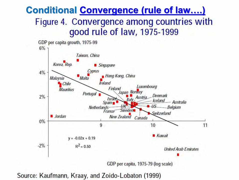
Conditional Convergence (rule of law….)

Conditional Convergence (Sachs & Warner...)
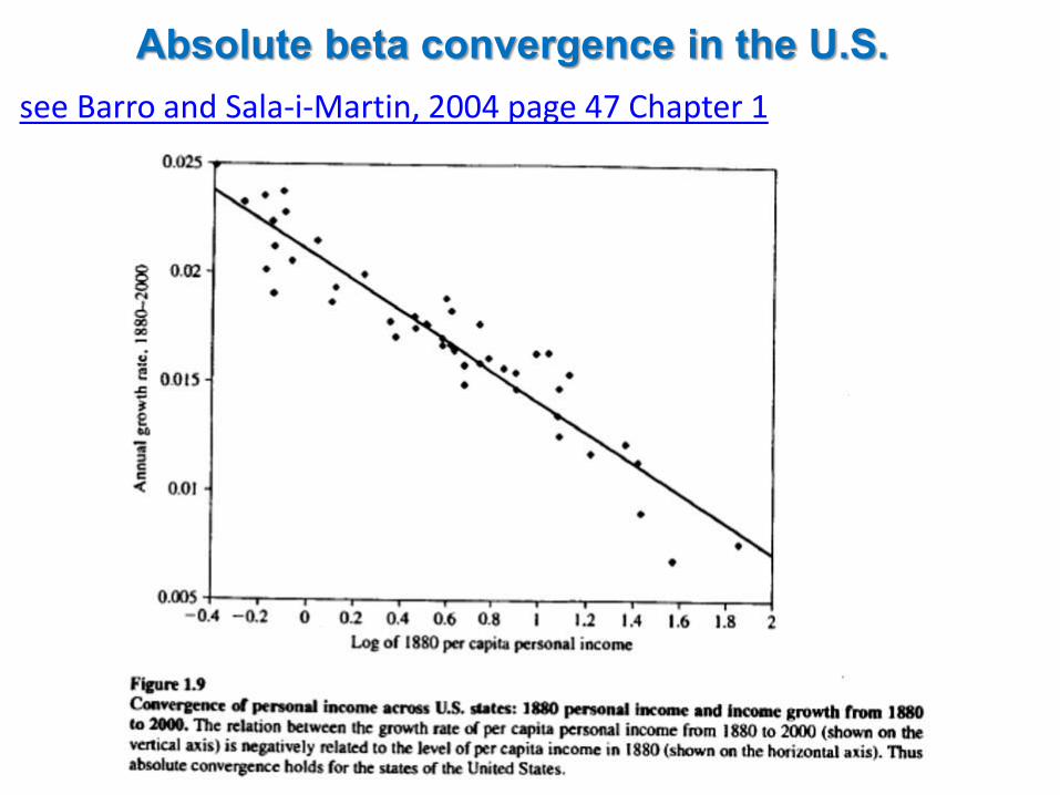
Absolute beta convergence in the U.S. see Barro and Sala-i-Martin, 2004 page 47 Chapter 1

Lack of absolute beta convergence
see Barro and Sala-i-Martin, 2004 page 45 Chapter 1
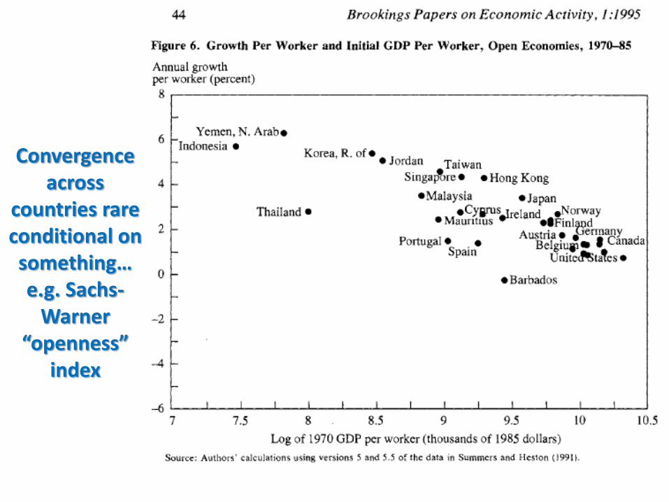
Convergence across
countries rare conditional on something… e.g. Sachs-
Warner “openness”
index
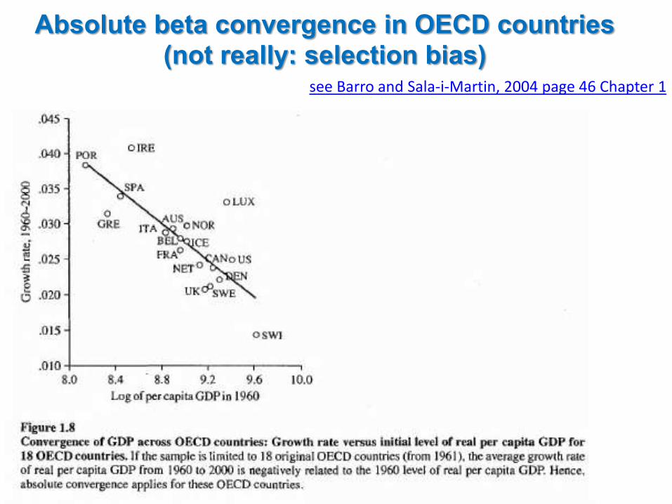
Absolute beta convergence in OECD countries (not really: selection bias)
see Barro and Sala-i-Martin, 2004 page 46 Chapter 1
Solow Swan Model takes TFP, aka A in y = Akα as given “exogenous”
• Endogenous growth theory models productivity growth.
• Learning by doing in the endogenous Chatterjee, Satyajit Making More out of less, recipe for long term growth, May/June 1994, Liberty Ships, page 10, Business Review, Federal Reserve Bank of Philadelphia
• http://www.phil.frb.org/research-and-data/publications/business-review/1994/brmj94sc.pdf

Solow Swan Model: growth rate diagram (see 3 growth models handout)
Long term growth rate
g* n + lsAka-1
Capital stockkL kH k* per worker
Figure 2Absolute Convergence
transtional growth
component
growth rate

Solow Swan Model: growth rate diagram (conditional convergence)
g* n + l
sAHka-1
sALka-1
Capital stockkL
k*L kH kH* per worker
growth rate
6%
5%
Figure 3Conditional Convergence

Solow Swan growth rate diagram (with everything…)
as k→0, mpk→∞
Growth Rate
Golden rule means α = s
mpk = αAka-1
3%
as k→∞, mpk→0
k* Capital stock per worker, k
Figure 5 Inada Conditionsand the Golden rule in the
Growth rate Diagram
γ = n + l

Exogenous Growth: Solow-Swan or “neoclassical Growth Model”
1. Key equations: y = Akα.
2. Key properties:
1. Convergence (absolute or conditional)
2. Technical change or TFP growth exogenous
3. Savings rate/pop growth affect steady state & ST growth, but do not affect LT Growth
3. Bottom line: more a model of “steady state” income levels than a theory of growth
4. Strengths: Augmented Solow model +

Exogenous Growth: Solow-Swan or “neoclassical Growth Model”
1. Key equations: y = Akα
2. Key assumptions:
1. Population growth exogenous, assume n.
2. Capital & labor substitutes
3. Savings rate exogenous (but there is “golden rule”)
3. Bottom line: more a model of “steady state” income levels than a theory of growth
4. Strengths: Augmented Solow + institutions can explain up to 90% of variation in income levels…
Endogenous Growth: HD to AK and beyond (R&D)
1. Key equations: y = Ak (see handout for Utility
2. Key assumptions: 1. Constant returns to capital and labor (e.g., when capital
& labor perfect substitutes– CES case below)
2. Savings rate endogenous function of IES 1/θ and discount rate ρ… so γ = (1/θ)(A-ρ)
3. Model technical change (except it AK model) as with learning by doing (LBD)
3. Bottom line: no “steady state” income level bit there is an endogenous steady state growth rate
4. Strengths: predicts constant growth rate, simple to apply and test….

Endogenous Growth: HD to AK and beyond (R&D) Barro and Sala-i-Martin,
2004 page 64 Chapter1
Exogenous or Endogenous Growth? Hybrid models:
1. Sobelo Model: y = Ak + Bkα an endogenous growth model that leads to conditional convergence (“transitional dynamics).
2. Villanueva Model : Agenor Chapter 12: a Solow model with endogenous technical change in which the savings rate matters for long run growth (not just transitional dynamics)
3. CES not Cobb-Douglas production function Solow model: endogenous growth with conditional convergence… this time due to an elasticity of substitution between K & L greater than one.

Hybrid model #1 Sobelo Model: y = AK + Bkα
see Barro and Sala-i-Martin, 2004 page 69 Chapter 1

Hybrid model #2 Villanueva Model :
see Agenor, 2004 Chapter 12
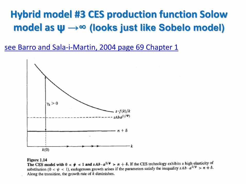
Hybrid model #3 CES production function Solow model as ψ →∞ (looks just like Sobelo model)
see Barro and Sala-i-Martin, 2004 page 69 Chapter 1

Demand side Poverty Trap with fixed costs -F modern technique is not competitive at T1 but out
performs at T2… see BSIM Chapter 1, p, 75
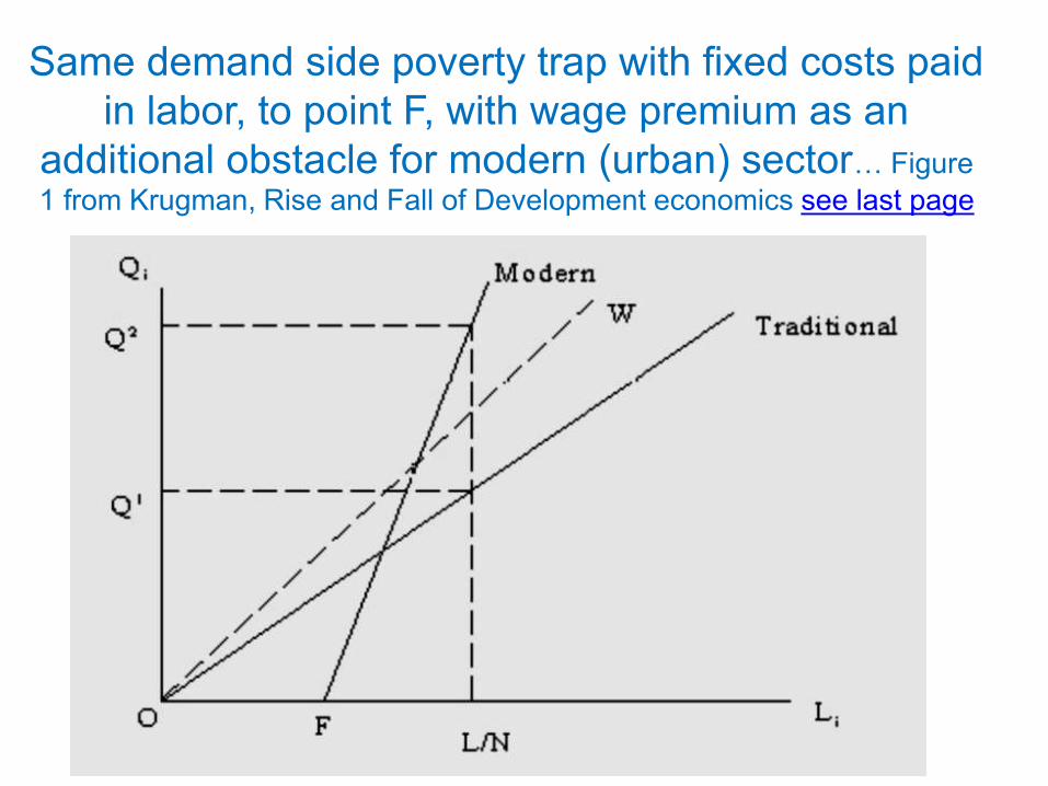
Same demand side poverty trap with fixed costs paid in labor, to point F, with wage premium as an
additional obstacle for modern (urban) sector… Figure 1 from Krugman, Rise and Fall of Development economics see last page

At Q2 the modern sector is profitable, at Q1 it is not, … See discussion of Figure 1 in Krugman, Rise and Fall of Development
eEonomics see last page
37
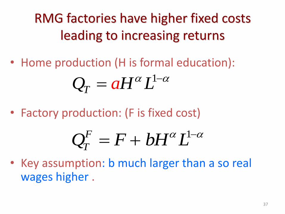
RMG factories have higher fixed costs leading to increasing returns
• Home production (H is formal education):
• Factory production: (F is fixed cost)
• Key assumption: b much larger than a so real wages higher .
1a a-T aQ H L
1F
TQ F bH La a-

38
h
Figure 8Market size poverty trap
real wage
h* Wage-
profitabilitythreshold
Traditional cottage-home
production dominates
(low wages- no fixed costs)
Poverty Trap ends: Modern Factory
production dominates
Factory with fixed cost F
Cottage-home Production
aFw = (1 - a)bh - rF
βCw = a(1 - β)h
-rF

39
Additional MFA quotas ends poverty trap, allows
factories to pay higher wages than traditional firms
h
An export quota poverty trap Figure 7
real wage
_
Lh(X )_
Hh(X )
T
D home lowQ = Q +X
TQ = Q +Xhome highD
aFw = (1 - a)bh - rF
βCw = a(1 - β)h
-rF

S-shaped Poverty Trap with increasing then decreasing returns createstwo steady states, k* low and k* high (not growth rate the same at both, a typo?) BSIM Ch 1p, 76

Demand side Poverty Trap Figure 5a Price, costs LRAC curve for Modern Industry
Figure 5a Demand-side poverty traps
Demand curve for closed economy….
MC = AC for traditional cottage industryP= MC MC t
MC factories marginal cost lower for modern
industry, has fixed costs too.
QA Quantity of output per firmWith inelastic demand, modern firms cannot compete (unless they outlaw competition-- perhaps with import tariffs or quotas + barriers to entry, expensive & hard to get business licenses or import permits)
with monopolistic competition Deardorff, Stern & Brown, 1993?

Demand side Poverty Trap Figure 5b Price, costs LRAC curve for Modern Industry
Figure 5b Demand-side poverty traps
Demand curve for Open economy….
MC = AC for traditional cottage industryP= MC MC traditional
marginal cost lower for modern MC factoriesindustry, has fixed costs too.
Quantity of output per firm QFT Quantity of output per firmWith more elastic demand in open economy, modern firms can compete, but average firm size increases and producitivy growsreducing employment (perhaps) and making traditional firms uncompetive, but costs fall and productivity of those still employed, average firm size after free trade is larger, economies of scale coverfixed and lower LRAC as traditional no fixed cost firms exit.
with monopolistic competition Deardorff, Stern & Brown, 1993?

Closed economy
demand side poverty Traps: evidence from Hsieh, Chang-Tai,
and Peter J. Klenow. 2010. "Development Accounting."
American Economic Journal: Macroeconomics, 2(1): 207-23, page
221, Figure 9
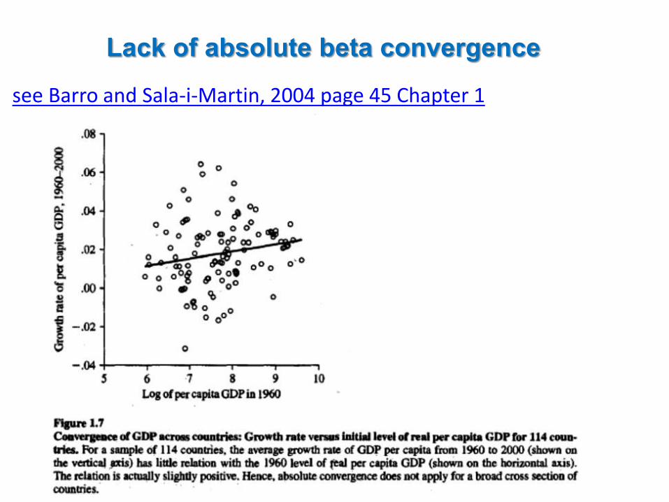
Lack of absolute beta convergence
see Barro and Sala-i-Martin, 2004 page 45 Chapter 1

Absolute beta convergence on OECD
see Barro and Sala-i-Martin, 2004 page 46 Chapter 1
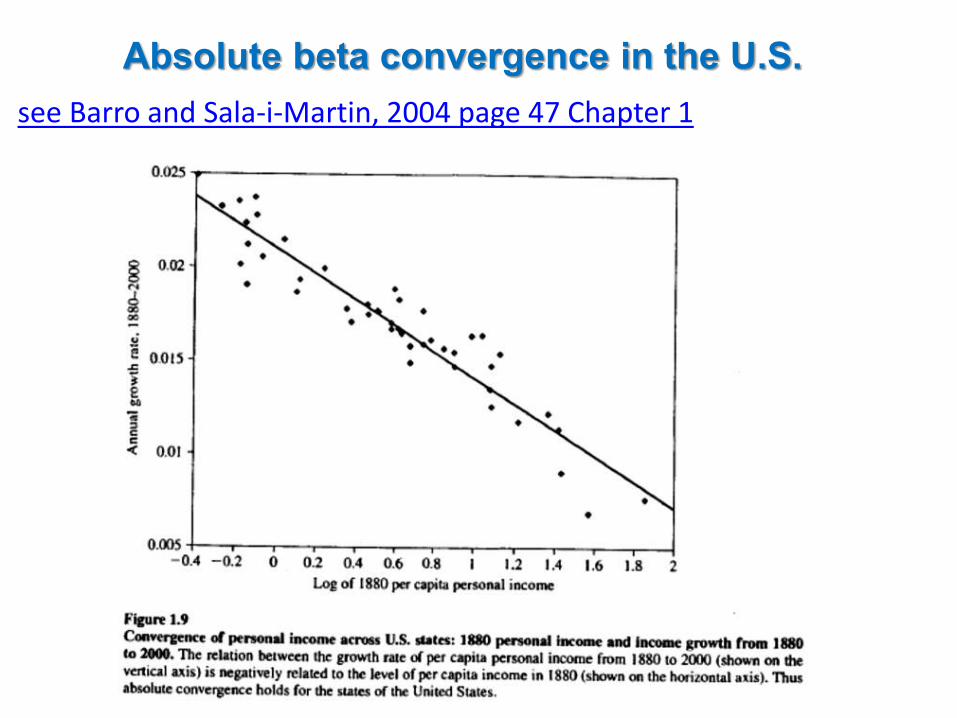
Absolute beta convergence in the U.S. see Barro and Sala-i-Martin, 2004 page 47 Chapter 1