Daniel Rodriguez Duque, David A. Stephens, Erica E.M ...
34
Estimation of Optimal Dynamic Treatment Regimes via Gaussian Process Emulation: A Technical Report Daniel Rodriguez Duque, David A. Stephens, Erica E.M. Moodie McGill University May 27, 2021 Abstract Causal inference of treatment effects is a challenging undertaking in it of itself; inference for sequential treat- ments leads to even more hurdles. In precision medicine, one additional ambitious goal may be to infer about effects of dynamic treatment regimes (DTRs) and to identify optimal DTRs. Conventional methods for inferring about DTRs involve powerful semi-parametric estimators. However, these are not without their strong assumptions. Dy- namic Marginal Structural Models (MSMs) are one semi-parametric approach used to infer about optimal DTRs in a family of regimes. To achieve this, investigators are forced to model the expected outcome under adherence to a DTR in the family; relatively straightforward models may lead to bias in the optimum. One way to obviate this difficulty is to perform a grid search for the optimal DTR. Unfortunately, this approach becomes prohibitive as the complexity of regimes considered increases. In recently developed Bayesian methods for dynamic MSMs, computational challenges may be compounded by the fact that at each grid point, a posterior mean must be calculated. We propose a manner by which to alleviate modelling difficulties for DTRs by using Gaussian process optimization. More precisely, we show how to pair this optimization approach with robust estimators for the causal effect of adherence to a DTR to identify optimal DTRs. We examine how to find the optimum in complex, multi-modal settings which are not generally addressed in the DTR literature. We further evaluate the sensitivity of the approach to a variety of modelling assumptions in the Gaussian process. 1 Introduction As our capacity grows to capture and store data, the questions we ask are to become more complex. In health research, ambitious data-guided questions may be asked in the quest for precision medicine where researchers seek to tailor treatment to patient-specific characteristics. This tailoring requires sets of decision rules, termed dynamic treatment regimes (DTRs), that take patient information as inputs, and that output a treatment recommendation. 1 arXiv:2105.12259v1 [stat.ME] 25 May 2021
Transcript of Daniel Rodriguez Duque, David A. Stephens, Erica E.M ...

Estimation of Optimal Dynamic Treatment Regimes via Gaussian
Process Emulation: A Technical Report
Daniel Rodriguez Duque, David A. Stephens, Erica E.M. Moodie
McGill University
May 27, 2021
Abstract
Causal inference of treatment effects is a challenging undertaking in it of itself; inference for sequential treat-
ments leads to even more hurdles. In precision medicine, one additional ambitious goal may be to infer about effects
of dynamic treatment regimes (DTRs) and to identify optimal DTRs. Conventional methods for inferring about
DTRs involve powerful semi-parametric estimators. However, these are not without their strong assumptions. Dy-
namic Marginal Structural Models (MSMs) are one semi-parametric approach used to infer about optimal DTRs
in a family of regimes. To achieve this, investigators are forced to model the expected outcome under adherence
to a DTR in the family; relatively straightforward models may lead to bias in the optimum. One way to obviate
this difficulty is to perform a grid search for the optimal DTR. Unfortunately, this approach becomes prohibitive
as the complexity of regimes considered increases. In recently developed Bayesian methods for dynamic MSMs,
computational challenges may be compounded by the fact that at each grid point, a posterior mean must be
calculated. We propose a manner by which to alleviate modelling difficulties for DTRs by using Gaussian process
optimization. More precisely, we show how to pair this optimization approach with robust estimators for the
causal effect of adherence to a DTR to identify optimal DTRs. We examine how to find the optimum in complex,
multi-modal settings which are not generally addressed in the DTR literature. We further evaluate the sensitivity
of the approach to a variety of modelling assumptions in the Gaussian process.
1 Introduction
As our capacity grows to capture and store data, the questions we ask are to become more complex. In health
research, ambitious data-guided questions may be asked in the quest for precision medicine where researchers seek
to tailor treatment to patient-specific characteristics. This tailoring requires sets of decision rules, termed dynamic
treatment regimes (DTRs), that take patient information as inputs, and that output a treatment recommendation.
1
arX
iv:2
105.
1225
9v1
[st
at.M
E]
25
May
202
1

Often, researchers are interested in asking causal questions about these DTRs. Most notably, what is the causal effect
of adherence to a specific DTR and what might the optimal DTR be. The search for an optimum is an important one
in medicine, as we want to avoid over-treatment, but we also want to provide sufficient care. Answering questions
about DTRs is challenging, even in data-rich environments; more data may correctly suggest we can ask tougher
questions, but the curse of dimensionality tells us that we cannot escape thinking about statistical models in order
to arrive at conclusions.
In the frequentist setting, inferential methods for dynamic treatment regimes have been traditionally performed
via semi-parametric models. These include dynamic marginal structural models (MSMs) [Orellana et al., 2010],
g-estimation of structurally nested mean models [Robins, 1986], Q-learning [Zhao et al., 2009] and outcome weighted
learning [Zhao et al., 2012]. For Bayesians, where modelling the entire probabilistic dynamics is often required
for inference, a variety of methods for DTRs have also been proposed, including Saarela et al. [2015], Murray
et al. [2018], Arjas and Saarela [2010], Rodriguez Duque et al. [2021], and Xu et al. [2016]. Though much of the
Bayesian literature in this area has focused on adapting existing frequentist estimation approaches for DTRs, the
computationally intensive nature of Bayesian inference limits their usability. In this work, we focus on eliminating
some of the modelling challenges with DTRs in order improve the usability of methods, be they frequentist or
Bayesian.
Our work is motivated by the use of Dynamic MSMs, where a Bayesian version was recently also proposed
Rodriguez Duque et al. [2021]. Dynamic MSMs allow for the estimation of the value of a DTR within a given family.
For example, researchers may posit the marginal mean model for the value of a DTR, g, where g belongs to a family
of DTRs indexed by r e.g. Y gψ
= β0 + β1ψ+ β2ψ2. Unfortunately, we cannot be certain that this model is correctly
specified, or that it will correctly identify the optimal regime within the family. This is exemplified by Appendix A
figure 1 where a quadratic fit to the data does not yield the true response surface and certainly does not identify the
optimizer. One way around this issue is to estimate the expected outcome under each regime in the family, if there is
a finite number of them, or to estimate the expected outcome of a large set of regimes and then extrapolate the value
to other regimes. This approach is particularly attractive as we have access to powerful estimators for the expected
outcome of these regimes. Unfortunately, this approach may require too much computation time, particularly in
settings with many stages, complex decision rules, and a variety of confounders. This computational challenge may
be exacerbated in Bayesian settings where computation is often a challenge. Though we focus on Dynamic MSMs,
this issue extends to methods beyond Dynamic MSMs. For example Xu et al. use g-computation along with non-
parametric models to identify an optimal regime in a small family. However, it is unclear how their method may be
used feasibly and robustly when the number of possible regimes is infinite.
Propitiously, there may be a way around this computational bottleneck by making use of well-designed computer
2

experiments with the aim of identifying outcome-optimizing DTRs. Though our focus will be on designing computer
experiments for alleviating the modelling issues with Dynamic MSMs and their Bayesian counterpart, this approach
can be connected to other estimation procedures. Traditionally, data-driven optimization was performed using a
regression-based approach termed response surface methods. However, these methods may not be well suited for
identifying optimal responses. Huang et al. mention that response surfaces may be inefficient as they attempt
to predict the response curve over the entire feasible domain, as opposed to in a neighbourhood of the optimum.
Additionally, regression models are usually relatively simple, and may not fit complex systems adequately over the
entire domain. Consequently, the literature has focused on a more modern approach using Gaussian processes (GP)
to perform computer experiments. A GP is a stochastic process for which all outcome vectors, regardless of the
dimension, are multivariate normally distributed. Models arising from the GP assumption are generally termed
Kriging models. These models are widely used in two settings: 1) researchers have access to data and they would
like to fit a flexible model, which may be used for prediction in unobserved locations 2) researchers are working with
a function that is expensive to evaluate and they would like to have a fast approximation of this function, thereby
minimizing the number of function evaluations needed to emulate the surface. Often, emulation is done for the
purpose of optimization. The latter is what falls into the computer experiments literature. What is unusual about
our setting is that computer experiments are usually applied to settings where the actual input output relationship
is known, just difficult to evaluate. In our setting, we only have access to the estimated response surface, and it is
the estimators that may be timely to evaluate. Effectively, this is a novel application of the methods.
Sacks et al. Sacks et al. [1989] were among the first works to explore using GP for computer experiments. Later,
Currin et al. Currin et al. [1991] used a similar methodology but in a Bayesian context. O’Hagan et al. O’Hagan
et al. [1999] argued that a Bayesian perspective was crucial for deterministic functions as, for fixed input, the output
does not change. Consequently, uncertainty about the response surface is epistemic, not aleatory thereby making
a frequentist approach haphazard. That being said, a fully Bayesian treatment of this problem is often highly
complex and some compromises must be made. We take this into consideration and seek practical methods that
find compromises between the Bayesian and Frequentist approach. One concern may be, as with any optimization
procedure, that there exist local maxima within the operating domain of interest, making the identification of a global
maximum more difficult. Jones et al. Jones et al. [1998] assuage these concerns by emphasizing that response surface
methodology is good for modelling non-linear multimodal functions. The GP assumption means that we must specify
a covariance and mean function. Additionally, as we hope to select points sequentially, we require an infill criterion;
a criterion which suggests what is the best place to sample from next, based on some desirable characteristics. There
are a variety of infill criteria in the literature. Most notably, the expected improvement criterion has been well
studied and is known to balance exploration of the input space with exploitiation of the optimizing region. Although
3

this is a great infill criterion, it does encounter theoretical problems in stochastic settings.
In the most straight forward setting, there are a variety of modeling choices in order to fully specify the GP
model. Most important are the choice of covariance kernel, and mean function related to the multivariate normal
distribution. Some authors have explored the use of covariance functions. For example, Simpson et al. found that
Gaussian correlation function performs well in 1,3, and 4 dimensional settings, and Matern correlation functions
perform well in two-dimensional problems. On the other hand Roustant et al. [2012] found that the Gaussian kernel,
which is infinitely differentiable, does not yield stable covariance matrices. Contrastingly, they found that the Matern
5/2 covariance kernel, which is twice differentiable, gives much better conditional covariance matrices. Beyond these
sorts of empirical investigations, there has been some work on model selection for Gaussian Processes, some of which
is reviewed in Shi and Choi, 2011.
What is unique about our approach is that we are looking to emulate an estimation surface as a means to
approximate the value surface of a family of regimes. Knowing the estimation surface is unbiased for the true
response surface, we examine whether the resulting emulated surface is also unbiased, in particular with respect to
the optimum. What is particular about this problem is that if we could use the estimator point-wise, we would
get a non-smooth curve, which is what poses difficulties with the value search approach. There are several reasons
as to why this lack of smoothness is present and indeed it is a finite sample issue. Contrastingly, as investigators,
we are likely interested in smoothing out this noisy curve, leading to a more interpretable model for prediction.
The consequence of this fact implies that we should consider GP model with an additional stochastic component.
Furthermore, there is no reason to think that the observed noise will be homoskedasatic about a smooth curve. There
are several sources of variability that may lead to heteroskedastic noise: 1) Measurement Error, possibly including
more variability in treatment arm than in response arm 2) Relatively smaller sample-size in some regions of the
regime input-space than others 3) Patient responses being more distant from the value function in some areas of the
input-space than others. We will more precisely exemplify these considerations in the in the following sections.
Now, the Kriging literature can be divided in two: settings with non-noisy observations and settings with noisy
observations. The former is relatively straighforward: there is a given input and a fixed output; the GP is a great
model for computer experiments in this setting. The setting of stochastic Kriging is somewhat more nuanced. Much
of the literature defines stochastic Kriging as emulating a response surface where at each experimental point the
output varies when re-evaluated at the same input. In settings that don’t involve sequential sampling of points this
definition is sufficient. However, when sequential sampling is required, more care should be taken in defining the
problem. There are some settings where we have a noisy function, as characterized by how jittery it is, but there
is no variability when re-evaluated. As [Forrester et al., 2006] puts it, there is no uncertainty in the output, even if
it is noisy around the true smooth curve. This nuance is certainly consequential when identifying infill criteria for
4

stochastic kriging. In some cases, we do gain information by re-sampling at the same data-point –in others we do
not.
There is much literature on stochastic Kriging, Picheny and Ginsbourger [2014] provide an overview of these
methods. There is also a growing literature on GPs with heteroskedastic noise. For example, Ankenman et al.
incorporate heteroskedastic noise by making the covariance model richer and then using plug in estimators. They
show that correctly accounting for both sampling and response-surface uncertainty has an impact on experiment
design, response-surface estimation, and inference. Frazier et al. also discuss heteroskedastic error and propose a
method for financial time series. [Yin et al., 2011] used kriging with a nugget effect, to allow for heteroscedastic noise
as they note that not accounting for noise in the Kriging model, estimates of covariance parameters may be highly
variable. They propose a modified nugget effect that seems to alleviate some of the issues with heteroscedasticity.
An interesting fully-Bayesian approach is presented by [Goldberg et al., 1997] which seeks to place a gaussian process
prior on the log noise level, yielding two gaussian processes priors. As mentioned above, a fully Bayesian treatment
is timely, but some work has been done on alleviating these issues. For example, Wang has looked at fast MCMC
procedures for gaussian processes with heteroskedastic noise. Thinking about practicality, [Kersting et al., 2007] follow
the same approach as Goldberg et al., however they do not use Monte Carlo and use a most likely heteroscedastic
Gaussian processes approach. Zhang and Ni offer an improvement on most likely heteroskedastic GPs. Jalali et al.
provide a comparison of kriging-based algorithms for optimization with heterogeneous noise. They adapt some of
the infill criteria, which were originally designed for homogeneous noise.
There are a variety of infill criterions. Huang et al. provide one way in which to use infill to sequentially sample
new points via an augmented expected improvement. Frazier et al. propose method for noisy data called knowledge
gradient. [Picheny et al., 2013] provides a review for noisy kriging methods and infill criteria. Most infill criteria
for stochastic settings seek to allow re-evaluations at already sampled points. However, this is not desirable in our
setting as we noted that there is no variability in the output. There are other technical issues in revisiting already
sampled points with the GP, for example ill-conditioned matrix. Frazier and Wang [2016] provide a brief overview of
Bayesian optimization for noisy and non-noisy data. Interestingly, they emphasize that the expected improvement
can actually lead to have some optimality results (for one extra sampled points), but this optimality disappears
in stochastic settings. Forrester et al. [2006] seeks to use the expected improvement criterion in noisy settings by
proposing a re-interpolation approach to optimization. This is the approach that we focus on.
Most work done on this sort of optimization has been done either though a frequentist lens, which is not well
supported, or via empirical Bayes. Besides the fully Bayesian approaches already mentioned, there has been work
on incorporating MAP estimation, for example as in Lizotte [2008].
5

1.1 Inferential Setting
We consider a sequential decision problem with K decision points and a final outcome Y to be observed at stage
K + 1. Decisions taken up to stage k give rise to a sequence of treatments zk = (z1, ..., zk), zj ∈ {0, 1}. At each
stage k, a set of covariates xk is available for decision-making and it is assumed that these consist of all time-fixed
and time-varying confounders. To denote covariate history up to time k, we write xk = {x1, ..., xk}. Subscripts are
omitted when referencing history through stage K. Then, all patient information is given by b = (x, z, y). We denote
a DTR-enforced treatment history by g(x) = (g1(x1), ..., gK(xK)). Our focus is restricted to deterministic DTRs.
Throughout, we will consider a family of DTRs, which will be indexed by ψ ∈ I to give G = {gψ(x);ψ ∈ I}. The
index is omitted when it is clear that our focus lies on a single DTR. We refer to the value function as the function
that takes as input ψ and returns E[ygψ
]. Point-wise evaluation of an estimator for the value function for a range of
ψ leads to what we term the estimator surface.
2 Background
Consider the following model:
υi = f(ψi) + εi with εi ∼ N(0, γ2(ψi)) (1)
Bayesian non-parametric inference allows us to place a prior dπ(f) on f ∈ F . Heuristically, we can consider the
following Bayesian updating equation:
P (f ∈ A|υ) =
∫A
Ln(f)dπ(f)∫F Ln(f)dπ(f)
, A ⊂ F (2)
This reflects the fact that there is epistemic uncertainty in the form of f . This problem is further complicated by
the fact that we may not get to observe f , but only a noisy version, namely υ. Indeed, the prior that we place is on
the value function. Available to us is the estimator function which we assume varies around the true curve. Now, to
make matters more concrete, suppose we have data D = {ψi, υi}ni=1, where ψi may be a p-dimensional column vector.
Then define the entire set of observations by ψ = (ψ1, ..., ψn)T , υ = (υ1, ..., υn) and f = (f1, ..fn). Furthermore, for
conciseness, we denote γ2 = (γ2(ψ1), ..., γ2(ψn)). Now, motivated by the Bayesian perspective, we place a Gaussian
process (GP) prior on the form of our function of interest f . This has the consequence that for any finite set of
observations ψ, f |ψ ∼ N(µ0f ,K). K is the covariance matrix calculated through a covariance function k(ψi, ψj),
usually dependent on parameters (θf , σ2f ). For example the Matern5/2 covariance:
k(ψi, ψj) = σ2f (1 +
√3|ψi − ψj |
θ) exp(
−√
3|ψi − ψj |θ
) (3)
Generally, then, the GP requires specifying a set of hyperparameters ηf = (µ0, θf , σ2f ). Without further knowledge of
the problem it is challenging to specify values for these hyperparameters. Specifying priors for these hyperparameters
6

is possible, but it may increases the computational issues. More commonly, empirical Bayes is used to estimate the
hyperameters, as exemplified in Shi and Choi [2011]. Alternatively, MAP estimation may be used. Regardless if MAP
or empirical Bayes, conditional on fixing these hyperparameters, standard arguments for the conditional distribution
of a multivariate normal distribution yield the posterior distribution to be:
fn+1|ψn+1, ηf , γ2,D ∼ N(µfn+1
, σ2fn+1
)
µfn+1 = µ0 + kT (K + S)−1(υ − µ0f )
σ2fn+1
= k(ψn+1, ψn+1)− kT (K + S)−1k
(4)
S is a diagonal matrix of noise variances with the ii entry equal to γ2i = γ2(ψi). From an empirical Bayes perspective,
the parameters are not random variable; they are fixed values. Consequently, they need not be included in the
conditioning, we do this however for compatibility with the MAP approach. Now, this model, unlike the more well
known GP model for computer experiments, does not interpolate the observed data. Meaning that, µfn+1does not
necessarily cross already observed sample points; it is a regressive model. This is desirable, as we are after a smooth
response curve, but we only have access to a noisy curve obtained from point-wise evaluation of the estimator. To
recover the interpolating model, we must just set γ2(ψi) = 0. As Forrester et al. [2006] point out, the interpolation
property of a GP occurs when there is no measurement error in the data observation mechanism and comes from
seeing that the posterior variance is zero at already sampled points, which is immediate from the following:
kTK−1k = k(ψi − ψi) = k(ψn+1, ψn+1). (5)
Furthermore, we note that with this model, which takes model parameters as given, the expression for the variance
at a new point differs from the frequentist literature which has an additional correction term. However, Forrester
et al. [2006] clarify that this correction term is negligible in practice. Consequently the discrepancy between the
frequentist and empirical Bayes approach is not particularly consequential. Lastly, the resulting posterior for the
noisy observations is:
υn+1|ψn+1, ηf , γ2, γ2
n+1,D ∼ N(µυn+1, σ2vn+1
)
µυn+1 = µfn+1
σ2υn+1
= k(ψn+1, ψn+1)− kT (K + S)−1k + γ2n+1
(6)
2.1 Homoskedastic Inference
We assume that the noise variance is homoskedastic, meaning γ2(ψi) = γ2,∀i. Now, if we had access to this model,
we could additionally combine it with MAP estimation in order arrive at an approximation for p(υn+1|ψn+1,D).
Then we could use this posterior predictive distribution to compute what will be clarified later as an expected
improvement measure, in order to complete our computer experiment. Overall, we are interested in computing
7

quantities in equation 4 and 6 in order to arrive at p(υn+1|xn+1,D). An empirical Bayes approach assumes all
hyperparameters are known and so p(υn+1|xn+1,D) = p(υn+1|xn+1, ηf , γ2, γ2
n+1,D), where marginalization has been
done over f . In actuality, these parameters are computed by maximizing the marginal distribution p(υ|ψ, ηf , γ2).
Note that γ2 is not actually a hyperparameter, but it is still maximized in the same way as in Shi and Choi [2011].
Efficient computational approaches to identifying the maximizers of this marginal likelihood can be found in Park
and Baek [2001] and Roustant et al. [2012].
Now, if we were interested in incorporating priors for some of the hyperparameter, we may do so via MAP
estimation and denote by ηmapf the maximizer of p(η|D). Then, MAP estimation assumes that p(η|D) ≈ 1ηmapf(ηf ).
This leads to the following approximation for the posterior predictive distribution:
p(υn+1|ψn+1,D) ≈ p(υn+1|ψn+1, ηmapf ,D) =
∫p(υn+1|ψn+1, ηf ,D)1ηmapf
(ηf )dηf (7)
Indeed we need not place a prior on each element of ηf . Shi and Choi [2011] mention that when non-informative
priors are used, MAP estimation is the same as empirical Bayes. Lizotte [2008] has examined MAP inference for
deterministic computer experiment under a log-normal prior for θ. We remind the reader that we seek to perform a
stochastic computer experiment.
2.2 Heteroskedastic Inference
Now, as we mentioned, there are reasons to believe the response surface exhibits heteroskedastic noise. Consequently
we review one approach for experimenting on data of this type. Following Zhang and Ni [2020], we model ei = log(γ2i )
with an independent Gaussian process with covariance function ke(ψi, ψj) and with parameters ηe = (µ0e, θe, σ2e).
Note that this is now an interpolating Gaussian process. For now, we are interested in performing the following
marginalization
p(υn+1|ψn+1, ηf , ηe,D) =
∫ ∫p1(υn+1|ψn+1, ηf , e, en+1, ηe,D)p2(e, en+1|ψn+1, ηe,D)deden+1
Based on our assumptions p2 is normal with posterior mean and variance as described in the general setup. If we
are using empirical Bayes, then ηf and ηz are not really hyperparameters; they are fixed values. Consequently this
marginalization is the right approach in order to arrive at a posterior predictive distribution. However, we note that
this marginalization does not work if we choose to incorporate hyperparameters and their priors. In that case p2 is
not the only term in the posterior dependent on e, and so this is not the correct posterior to integrate over. Literature
has termed this approach Most Likely Heteroskedastic GP Regression. Indeed, then, this Heteroskedastic approach
is more amenable to an empirical Bayes approach and does not lend itself very coherently to MAP estimation of the
hyperparameters. As we will note, though, this approach very much resembles MAP inference with regard to the
distribution of the posterior error variances. First, we make an important observation: we do not have access to data
8

e1, ..., en. We later review how these can be estimated, but for now we proceed as if they were known. Now, using
the following approximation: p(e, en+1|xn+1, ηe,D) ≈ δ(e, e∗), where e, e∗ denote the maximizers of p2 leads us to:
p1(υn+1|ψn+1, ηf , ηe,D) =
∫ ∫p(υn+1|xn+1, θf , e, en+1,D)1(e,en+1)(e, en+1)dzden+1
≈ p(yn+1|ψn+1, ηf , ηe, e, en+1,D).
(8)
Consequently, the right hand of the equation above tells us that the posterior that we are interested in can be
approximated by a Gaussian Process with mean and variance given in equation 6, where γ(ψi)s are replaced with
eis. As we mentioned, data on e1, ..., en is needed in order to infer about the second GP. In short, this requires
obtaining the residuals of a GP model fit on data υ1, ..., υn and fitting the second GP to a transformation of these,
the full procedure being laid out in Zhang and Ni [2020].
We now have regressive homoskedastic and heteroskedastic models for the desired response surface. This is
excellent, except for the fact that now it becomes a challenge to use traditional infill methods like the Expected
Improvement method to be defined later. In particular, in order to guarantee that the expected improvement identify
the true optimum as the number of experimental points increases, we need the posterior variance in already sampled
locations to be zero [Forrester et al., 2006] [Locatelli, 1997]. This is a reasonable requirement because although we
know there is error in the sample locations, we know that in our setting there is no uncertainty in the result. This
property is achieved by obtaining an interpolating surface through the values predicted by the GP regression at the
sampled locations.
2.3 Re-interpolation
The re-interpolation methods allows us to place a GP prior on the posterior mean of the analysis above. In particular,
we are saying that the posterior mean does not vary when re-evaluated at the posterior outcome. This is the essense
of the reinterpolation model presented by Forrester et al. [2006]. Simply, this model uses the predictions of the mean
of υn+1|ψn+1,D, call these (υ1, ..., υn) in order to obtain a new dataset D′ = {ψi, υi}ni=1. Then we obtain a similar
heuristic as before:
p(υn+1|ψn+1,D′) = p(υn+1|ψn+1, ηf ,D′) (9)
Note that the hat in ηf is not used to indicate an estimated quantity, but rather the the parameter belonging to
the v process. Now, the main idea behind this is that the mean of the υ and υ processes are the same, while the
variance of the υ process possesses the characteristics that we are after: it is zero at already sampled points. K and k
remain unchanged, so θ is not re-optimized [Forrester et al., 2006]. The reinterpolation approach has not previously
been used in a heteroskedastic noise setting, so we show that it still applies in Appendix A. In particular, it must
9

be that µ0υ = µ0υ. We note that this approach only works from an empirical Bayes’ approach on the prior mean.
Otherwise, a MAP approach that in includes a prior for the mean would yield a different equations for the posterior
means.
2.4 Infill Criteria
Then, we return to the question of an appropriate infill criterion when we are interested in performing minimization.
The expected improvement in our setting is given by: E[I(ψ)] = E [max(υmin − υ(ψ))+|D′]. The expectation is
taken with respect to the posterior distribution and υmin = min(υ1, ...υn). Further computation yields: E[I] =
(υmin − µυ(ψ))Φ( υmin−µυ(ψ)συ(ψ) ) + συ(ψ)φ( υmin−µυσυ(ψ) ) when συ(ψ) > 0 and 0 otherwise. Φ is the CDF of the standard
normal distribution and φ is the corresponding pdf. We can see from this expression how exploitation and exploration
are balanced.
2.5 Design of Experiments
There are a variety of ways to select design points, we simply select them equally spaced within dimensions. Sometimes
points are selected at random, but given the nature of our experiment, we want to eliminate variability due to the
initial sample, and focus on the variability due to the esimation surfaces. Additionally, this makes optimization
somewhat easier by reducing the variability of initial fits.
Another design choice that must be made is the covariance function. Choosing the covariance parameter is an
important element. Some covariance function lead to smoother surfaces versus others, for example the sample paths
of the associated Gaussian process have derivatives at all orders and are thus very smooth. Another common choice
of covariance is the Matern covariance, which is mean square differentiable up to order k. Common choices are the
Matern 5/2 covariance which is twice differential and the Matern 3/2 covariance which is differentiable once. These
are also examples of anisotropic covariance functions, meaning that the curvature of the function may differ across
directions.
Martin and Simpson mention that there are three issues in maximization. Ridges in the likelihood, multiple local
optima, and ill-conditioned matrices. Stein mention that using Matern covariance, models they are unaware of any
model that leads to multiple optimizers, however we have observed multiple optima in the non-interpolating model
scenario. Davis and Morris determined that larger correlation ranges and closer located observations tend to result
in larger condition numbers, a measure of the stability of a matrix inverse. We also found this in this work. Sasena
used a nugget effect to alleviate issues with ill-conditioned matrices.
10

2.6 Estimation Surface
We focus on the IPW estimator, which can be evaluated on a grid of ψs in order to give the resulting estimation
surface. The frequentist estimator is given by
1
n
∑i
wψyi (10)
where,
wψ =1gψ(x)(z)∏K
j=1 pO(zj |zj−1, xj−1, b).
Clearly, as the complexity of 1gψ(x)(z) grows, performing a grid search on the resulting IPW surface becomes
prohibitive. Additionally, this is not taking into account the non-smoothness of the IPW surface, which can possibly
hinder the correct identification of an optimum.
Now an additional layer of complexity is encountered if we would like to perform Bayesian inference. Denoting
by ∗, a draw from the posterior distribution, then the quantity we are after is:
Egψ [y∗|b] = EO[w∗ψy∗|b] (11)
where,
w∗ψ =1gψ(x∗)(z
∗)∏Kj=1 pO(z∗j |z∗j−1, x
∗j−1, b)
.
The right hand expectation is taken with respect to the posterior distribution in the observational world data
generating mechanism. Under a non-parametric prior specification on the family of data generating distributions
in the observational world, PF , we may compute a posterior by sampling a distribution from the non-parametric
posterior, computing the expectation and averaging through, as in:
EF [E[w∗Y |b,F ]] (12)
A robust, non-informative choice of prior in the observational measure is the non-parametric Dirichlet process
(DP) prior, with posterior asymptotically concentrating around the true data generating distribution. In par-
ticular, when DP(α,Gx) is chosen such that |α| → 0, we obtain the non-parametric Bayesian bootstrap as the
posterior predictive distribution. Under this specification, one sample drawn from the posterior DP is given by
p(b∗|b,Π) =∑ni=1 πi1bi(b
∗), where Π = (π1, ..., πn) ∼ Dir(1, ..., 1) is a sample from the Dirichlet distribution with
all concentration parameters equal to one. Under the Bayesian bootstrap assumptions, any distribution sampled
from the posterior DP is uniquely determined by Π. To compute functionals of the posterior predictive, we require
p(b∗i ∈ A|bi) = EΠ[p(b∗i ∈ A|bi,Π)] which may be estimated by resampling weights (π1, ..., πn) from Dir(1, ..., 1), and
computing the average over all samples. Consequently, under the Bayesian bootstrap assumptions, we are able to
compute the expected posterior experimental world utility via:
EF [E[w∗Y |b,F ]] = EΠ[E[w∗Y |b,Π]] = EΠ[∑i
πiw∗i yi] (13)
11

Details of this approach can be found in Rodriguez Duque et al. [2021]. It happens that under the Bayesian bootstrap
prior, the mean value of the estimated regime is identical to the frequentist approach. For this reason, we focus on
solving the IPW estimator. However, there are many other non-parametric priors that may be set, and most of these
would require sophisticated MCMC methods to obtain a regime’s value at each point. This further emphasizes that
a fully Bayesian treatment of the proposed problem requires even more computational power at each grid point,
thereby cementing the need for a computer experiment methodology.
2.6.1 Sources of Variation
As we have already discussed, the estimation curves exhibit some interesting sources of variation, and this should
be taken into account. In this section, we examine some of the possible sources of heteroskedastic variation that we
may wish to account for in our modeling approach. We note additionally that Case I and II would only lead us to
adapt our modeling strategy in finite samples. In this exploration, we limit ourselves to regimes of the form treat if
x > ψ, as this is a common regime in the literature, and it has straightforward, interesting exemplary properties.
It turns out that this is a very useful regime to consider, as it leads to clear examples about how heteroskedasticity
is manifested. Irrespective of the data generating mechanism, so long as it depends on binary treatment, we will
observe two response curves: the treated curve and the untreated curve. What we must realize is that as ψ increases,
only treated patients become non compliant and only untreated patients become compliant. Furthermore, for an
increase from ψ1 to ψ2, only patients with covariate values ψ1 ≤ x1 ≤ ψ2 are eligible to become compliant/non-
compliant. Of course, notice that in contrast to static treatment regimes, an individual can be simultaneously
compliant with many many DTRs. These properties are important in examining the variability in the following.
The first case we consider is heteroskedasticity due to distance from regime response surface. The first source
of heteroskedasticity relates to how close/far the treated and untreated lines are from the regime response surface.
Consider the family of regimes: treat if x > ψ;ψin. For a change from ψ1 to ψ2, there will be a set of patients who
become non-compliant with regime ψ2 and a set who become compliant. If either the newly compliant/non-compliant
patients have a response value that is far away from the population level regime estimator, then these observations
will have a lot of influence over the curve, specially for relatively small sample sizes. If the observations tend to
have a response that is near the population average, then the IPW surface will exhibit less influence from these
observations. Newly adherent or non/adherent patients tend to have similar outcome values as they have similar
covariate values (this is why they become compliant or not). Appendix A shows an explicit example of this.
The second case is heteroskedasticity due to heteroskedastic noise at the individual level. Now, a natural source
of noise in the estimator surface is heteroskedastic noise at the individual level. We examine this specifically with
respect to the IPW estimator. If we consider an additive error term like :z1ε1 + (1 − z1)ε2), where ε1 = N(0, 5),
12

ε2 = N(0, 0.5). We might not think this is an issue, as for estimation via an estimating equation; it does not
matter whether noise is heteroskedastic or homoskedastic, so long as it has zero mean. However, when attempting
to estimate a response curve for the purposes of identifying a minimum, this may be consequential. Again if we
consider regimes of the form x1 > ψ, what we should recall that as ψ increases, we lose treated patients, and we gain
untreated patients. This means that we are losing observations with high variability and gaining observations with
low variability. In appendix A, we show an example of this, including the resulting heteroskedasticity in the estimator
surface. Now, we may ask when it is reasonable to have such a data-generating mechanism, and in fact, whether
it’s possible to have such an error structure. It is not unreasonable to assume that there is a different stochastic
component for treated and untreated patients. Treatment may lead to relatively reliable improvements, but lack of
treatment may lead to disease progression taking on a variety of forms, and therefore leading to higher variability.
The last consideration that may lead to heteroskedasticity in the estimation surface is the result of differing
effective samples sizes across values of ψ. It is well known that the IPW estimator for a regime ψ only uses patients
who are compliant to the regime. Consequently, different regimes will use different number of patients to compute
the value of the corresponding regime. This means that the estimator will exhibit differing levels of variability for a
range of ψs. In appendix A, we show an example where this is the case.
3 Simulations
There are a variety of metrics that can be used to evaluate the performance of a Gaussian Process model. suggested
by Sasena (This thesis also has good example of monotonic likelihood. Page 53.). Some previously suggested metrics
are 1) f1 metric: The number of iterations required before a point is sampled with an objective function value within
1 percent of the true solution 2) x1 metric: The number of iterations required before a point is sampled within a box
the size of plus/minus 1 of the design space range centered around the true solution 3) xstar metric: The Euclidean
distance from the best sample point to the global solution.
3.1 Identification of Locally Optimal Regimes
When performing simulations involving DTRs, it is common to pose a data generating mechanism via regret functions,
as opposed to blip functions. However, in a multi-modal setting is unclear how blips may help us, as it is unclear
how to identify the optimal regime. For now, we focus on data-generating mechanisms based on blips, which has the
added benefit of having a simpler form for the outcome.
If we explore rules of the form treat if x > ψ and if the data-generating mechanism is of the form Y = x1+z1g(x1),
then the globally optimal regime is still relatively straightforward to identify: treat if g(x1) > 0. However, depending
13

on the form of g(x1), it is likely that this regime will not be in the family of interest, and may not be clinically
meaningful or straightforward to implement. This makes the issue of identifying the regime in the family sightly
more complex. In the family of interest, the optimal threshold ψ∗ is the one that maximizes∫∞ψg(x)f(x)dx. When
g(x) is a polynomial, computing these integrals should not be too difficult. In fact, in some cases the optimum
should be obvious from the plot of g(x)f(x), as the integral is the area under this curve. We look for the regime
that maximizes or minimizes this area. Of course, we note that the distribution of x dictates the form of the value
function, and consequently of the optimal regime in the family. This contrasts the case with the global optimum
which is invariant of the distribution of x.
3.2 Simulation I: Single Stage Example
The simulation setup is as follows, we used a sample size of n=1000, to generate covariate x1 ∼ U(−1.5, 1.5),
treatment z1 ∼ Binom(p = expit(2x1)), error distributions ε1 = N(0, σ = 0.25) ε = N(0, σ = 0.05) and final
outcome y = −(x1 + .8) ∗ x1 ∗ (x1 − .9)z1 + z1ε1 + (1 − z1)ε2. We explored the regime x1 > ψ, ψ ∈ (−1.5, 1.5).
With this data-generating mechanism, the systematic component of y varies from -2 to 2.5. The optimal regime
represents a 5 % improvement (in the range of y) over the worst regime in the class. In figure 1, we observe the
value function for this problem and the result of a point-wise estimation of the IPW estimator for each ψ, across
multiple replicates. It is visually evident that the function has two local minima, but only one global minimum at
0.9. Contrary to common belief, a grid search for the minimum may not work well, as evidenced from panel (b).
Though this is a bimodal problem that emphasizes the issue with grid search, can think that the issue also existing
more locally around the optimum.
The computer experiment was setup such that 15 equidistant points were taken to fit the initial model. Then,
additional points were taken up to 25 additional points. To perform statistical comparisons, we performed 150
replications for each procedure. We attempted to compare the results for models assuming no noise, homoskedastic
noise, and the heteroskedastic method described previously. In the following tables, all standard errors are Monte
Carlo standard errors. Confidence intervals for the minimizing ψ are produced by multiple draws from the posterior
multivariate normal distribution with appropriate mean and covariance. For each curve drawn from the multivariate
normal, a grid search was performed to identify the minimum. This results in a distribution of minimums. Note
that the grid search is only necessary if we are interested in confidence intervals. Otherwise, the minimizer from
the EGO algorithm. Note that the min from the EGO algorithm is not necessarily exactly the min of the posterior
mean; EGO algorithm only considers points to be minimizers from the set of visited points, this is different from
identifying the min by doing a grid search on the posterior mean.
14
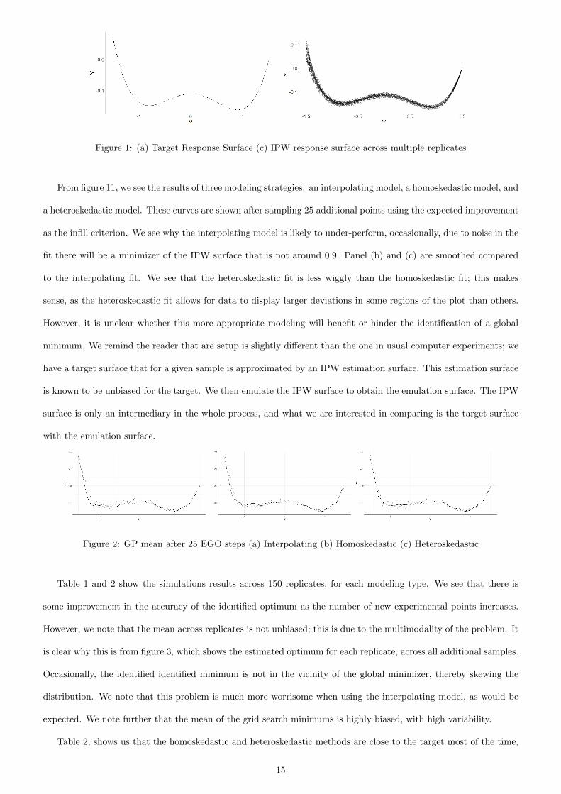
Figure 1: (a) Target Response Surface (c) IPW response surface across multiple replicates
From figure 11, we see the results of three modeling strategies: an interpolating model, a homoskedastic model, and
a heteroskedastic model. These curves are shown after sampling 25 additional points using the expected improvement
as the infill criterion. We see why the interpolating model is likely to under-perform, occasionally, due to noise in the
fit there will be a minimizer of the IPW surface that is not around 0.9. Panel (b) and (c) are smoothed compared
to the interpolating fit. We see that the heteroskedastic fit is less wiggly than the homoskedastic fit; this makes
sense, as the heteroskedastic fit allows for data to display larger deviations in some regions of the plot than others.
However, it is unclear whether this more appropriate modeling will benefit or hinder the identification of a global
minimum. We remind the reader that are setup is slightly different than the one in usual computer experiments; we
have a target surface that for a given sample is approximated by an IPW estimation surface. This estimation surface
is known to be unbiased for the target. We then emulate the IPW surface to obtain the emulation surface. The IPW
surface is only an intermediary in the whole process, and what we are interested in comparing is the target surface
with the emulation surface.
Figure 2: GP mean after 25 EGO steps (a) Interpolating (b) Homoskedastic (c) Heteroskedastic
Table 1 and 2 show the simulations results across 150 replicates, for each modeling type. We see that there is
some improvement in the accuracy of the identified optimum as the number of new experimental points increases.
However, we note that the mean across replicates is not unbiased; this is due to the multimodality of the problem. It
is clear why this is from figure 3, which shows the estimated optimum for each replicate, across all additional samples.
Occasionally, the identified identified minimum is not in the vicinity of the global minimizer, thereby skewing the
distribution. We note that this problem is much more worrisome when using the interpolating model, as would be
expected. We note further that the mean of the grid search minimums is highly biased, with high variability.
Table 2, shows us that the homoskedastic and heteroskedastic methods are close to the target most of the time,
15

even only after five additional points have been sampled. The interpolating model does not perform as badly, when we
consider the median, but we note that the variability is much higher than in the other two methods. It also does not
improve with increasing experimental points. Even the grid search is closer to target in this case, though not quite,
but the variability is two orders of magnitude higher than the magnitude of the homoskedastic and heteroskedastic
methods.
The converge column in the tables indicate how many replications, out of the 150, completed without issue.
Ideally, this would be all replications, but given the nature of the problem there are a few issues that can arise
when performing optimization using these models. In a real-data analysis setting these issues can be remedied
in straightforward says. Issues that can arise include 1) ill-conditioned matrices because the infill criteria suggests
multiple nearly identical points or 2) likelihoods that have a very shallow maximizer, or with score values asymptoting
to zero, thereby throwing off the optimization algorithm. These are solvable by adding a small nugget effect to the
covariance matrix or by being more careful about domain of optimization. Of course, across replications this is not
feasible. That being said most of our simulations completed without issue, and so there is no cause for concern. We
did observe, however, that when the noise in the problem increases, to perhaps unrealistic levels, the proportion of
models that do not converge increases as well.
Table 1: Optimal threshold ψ for Matern 5/2 covariance, with constant mean (Known optimizer: 0.9). Grid search
minimizer: 0.26 (0.838).
Mean (SD) +1 Point +5 Points +10 Points +15 Points +20 Points +25 Points Number Converge
Interpolating 0.614 (0.628) 0.639 (0.612) 0.613 (0.627) 0.614 (0.631) 0.576 (0.669) 0.531 (0.704) 150
Homoskedastic 0.717 (0.539) 0.769 (0.465) 0.826 (0.356) 0.818 (0.365) 0.814 (0.372) 0.794 (0.413) 148
Heteroskedastic 0.703 (0.546) 0.773 (0.457) 0.803 (0.399) 0.778 (0.446) 0.803 (0.402) 0.776 (0.447) 144
Table 2: Optimal threshold ψ for Matern 5/2 covariance, with constant mean (Known optimizer: 0.9). Grid search
minimizer: 0.83 (1.68).
Median (IQR) +1 Point +5 Points +10 Points +15 Points +20 Points +25 Points Number Converge
Interpolating 0.857 (0.138) 0.857 (0.145) 0.857 (0.148) 0.857 (0.141) 0.857 (0.152) 0.857 (0.163) 150
Homoskedastic 0.857 (0.076) 0.893 (0.079) 0.897 (0.08) 0.898 (0.082) 0.894 (0.081) 0.895 (0.068) 148
Heteroskedastic 0.857 (0.071) 0.89 (0.073) 0.894 (0.072) 0.898 (0.076) 0.9 (0.072) 0.893 (0.072) 144
Table 3 and 4, show the consequences of estimating procedure on the value of the optimal regime. We see that
in this case, the grid search values, does not deviate as much as the grid search optimum. This is because the two
minima in the function have similar values. However, we do note that the grid search still does exhibit more bias
16

than the homoskedastic and heteroskedastic approaches. Interestingly, unlike for the optimal regime, the estimation
of the value does not really improve substantially with additional experimental points.
Table 3: Value at optimal threshold ψ for Matern 5/2 covariance, with constant mean (Known value: -0.1649). Grid
search value: -0.177 (0.015) .
Mean (SD) +1 Point +5 Points +10 Points +15 Points +20 Points +25 Points Number Converge
Interpolating -0.169 (0.016) -0.171 (0.016) -0.172 (0.015) -0.173 (0.015) -0.173 (0.015) -0.174 (0.015) 150
Homoskedastic -0.167 (0.015) -0.167 (0.015) -0.167 (0.014) -0.167 (0.015) -0.167 (0.014) -0.167 (0.014) 148
Heteroskedastic -0.167 (0.015) -0.167 (0.015) -0.167 (0.015) -0.167 (0.014) -0.167 (0.014) -0.167 (0.014) 144
Table 4: Value at optimal threshold ψ for Matern 5/2 covariance, with constant mean (Known value: -0.1649). Grid
search value -0.176 (0.021) .
Median (IQR) +1 Point +5 Points +10 Points +15 Points +20 Points +25 Points Number Converge
Interpolating -0.169 (0.019) -0.171 (0.021) -0.172 (0.02) -0.173 (0.021) -0.173 (0.021) -0.173 (0.021) 150
Homoskedastic -0.169 (0.02) -0.167 (0.019) -0.167 (0.019) -0.167 (0.02) -0.167 (0.02) -0.167 (0.019) 148
Heteroskedastic -0.167 (0.019) -0.167 (0.02) -0.167 (0.02) -0.168 (0.019) -0.167 (0.019) -0.167 (0.019) 144
From table 5, we see that the coverage probability for the optimal regime. It is uncommon for literature on
computer experiments to present any coverage probabilities. This may be because it is computationally expensive
to do so. For this reason, we only present intervals for five additional points and for 25 additional points. We
see that the intervals for the homoskedastic method are closer to nominal than the approach that acknowledges
heteroskedasticity. This may be because the variance close to the optimum is smaller than the overall variance,
thereby making confidence intervals smaller. This table also shows that increasing the number of experimental
points, increases the coverage; this is more to do with accuracy increasing with an improving model.
Table 5: Coverage probability for 95% confidence intervals across 150 replications
+5 Points +25 Points
Interpolating 0.88 0.99
Homoskedastic 0.92 0.97
Heteroskedastic 0.76 0.82
In appendix B, we show results for a variety of different setups, including smaller sample sizes, a different
covariance function, and a log normal prior on the covariance parameter θ.
17
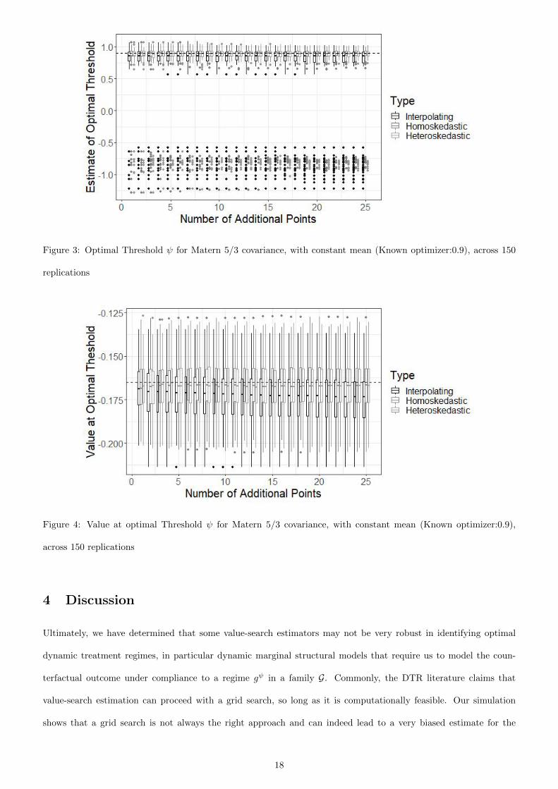
Figure 3: Optimal Threshold ψ for Matern 5/3 covariance, with constant mean (Known optimizer:0.9), across 150
replications
Figure 4: Value at optimal Threshold ψ for Matern 5/3 covariance, with constant mean (Known optimizer:0.9),
across 150 replications
4 Discussion
Ultimately, we have determined that some value-search estimators may not be very robust in identifying optimal
dynamic treatment regimes, in particular dynamic marginal structural models that require us to model the coun-
terfactual outcome under compliance to a regime gψ in a family G. Commonly, the DTR literature claims that
value-search estimation can proceed with a grid search, so long as it is computationally feasible. Our simulation
shows that a grid search is not always the right approach and can indeed lead to a very biased estimate for the
18

optimum. We have shown that a Gaussian optimization approach that accounts for variability in the estimated
response surface more accurately and precisely estimates the optimal DTRs of interest. In the appendix, we further
illustrated that the resulting success of the homoskedastic and heteroskedastic approaches are maintained for smaller
samples sizes and differing modeling decisions.
A Appendix A: Heteroskedasticity
For all examples relating to heteroskedasticity, we focus on regimes of the form treat if x > ψ. We refer to the value
surface, as the surface produced by evaluating the value of a regime ψ for a range of ψs. We refer to the IPW surface
as the surface that arises from point-wise evaluation of an estimator for the value of a regime ψ for a range of ψ. As
described in the main text when going from regime ψ1 to regime ψ2 (ψ1 < ψ2), we can only lose treated patients
and gain untreated patients.
A.1 Heteroskedasticity Type I
The first source of heteroskedasticity is interesting and unexpected. Mainly, it relates to the fact that patient-level
responses can exhibit substantially higher levels of variability than the regime value surface. We consider the following
data generating mechanism for the purposes of illustration.
• Y = 1000(−x1 + (x1 + 0.8)x1(x1 − 0.2)(x1 − 0.4)(x1 − 0.8)z1)
• n = 10000, x1 ∼ U(−1, 1), z1 ∼ bin(1, 0.5)
Note that y|x1, z1 is deterministically generated so as to avoid other sources of variability. In panel (a) of figure 5,
we see the mean response for the treated and untreated patients, as well as the regime value surface. We note that
in this scale, the surface looks flat, but it is actually multi-modal. In panel (b) of 5, we observe the IPW estimation
surface, and we that there are clear signs of heteroskedasticity. Most notably, there is much more variability in
the edges of the plot than in the middle. This variability depends mainly on three things 1) How close are the
treated and untreated lines to the IPW surface 2) How many people become compliant 3) How many people become
non-compliant.
It is clear from figure 5 that the IPW exhibits less variability around zero. This corresponds to when the treated
and untreated lines are closest to the IPW surface. Conversely, when the lines are far from the IPW surface, more
variability is observed. We may ask ourselves why there should be more variability if, in some cases, the treated line
and the untreated lines are proximal to each other. In the presence of confounding, this arises because more treated
patients are being lost than untreated patients. Now, in an unconfounded setting, for an increase in ψ, the number of
19

lost non-compliers is the same as the number of new compliers, on average. However, for a given finite sample there
may be more/less new compliers than non-compliers, and it is these differences that lead to variability in the curve,
even if treated and untreated response lines are similar. Now, this is mainly a finite sample issue. As more patients
contribute to the IPW estimator, it becomes harder to shift the mean by a large amount when a small number of
patients are added or taken away.
Figure 5: (a) Value surface and treated/untreated response curves (b) IPW estimation surface with treated and
untreated response
A.2 Heteroskedasticity Type II
We consider a simple data-generating mechanism that illustrates clearly that indeed heteroskedasticity does surface
at the estimator level.
• n = 1000, ε1 = N(0, 5), ε2 = N(0, 0.5)
• Homoskedastic Mechanism: y = 100(−2x1 +O1z1 + ε1)
• Heteroskedastic Mechanism: y = 100(−2x1 + x1z1 + z1ε1 + (1− z1)ε2)
• x1 ∼ U(−10.5, 10.5) z1 ∼ binom(1, 0.5)
Again note that there is no confounding in this setup. This is done on purpose, as it ensures that the number of units
adherent to each regime is the same across ψ. For the IPW estimator, conditional on known treatment propensity,
variance is related to the number of units adherent to a treatment; we refer to this as the effective sample size. As we
will see in Case III, confounding plays a role in the effective sample size and consequently on the variability structure.
Indeed, we observe that the variability of the IPW surface is heteroskedastic. We see from figure 6 that when there
is homoskedastic noise in the person-level mechanism, this transfers to homoskedastic noise in the IPW estimator.
The noise only plot is create by taking the weighted mean of the noise terms only. It is quite straightforward to see
why heteroskedasticity comes about for regimes of type treat if x1 > ψ. We have already established that, as we
move from left to right in the plots above, we lose treated patients and gain untreated patients. This means that
we are losing observations with high variability (ε1), and gaining observations with low variability (ε2). This has
the consequence of affecting the variability of the resulting estimator. Note that in this example, IPW weights were
computed with known treatment propensities.
20

Figure 6: n=1000 (a) IPW estimator; homoskedastic case (b) IPW estimator; heteroskedastic case; (c) Noise Com-
ponent of heteroskedastic case
A.3 Heteroskedasticity Type III
Now we exemplify how variability is a function of sample size, in particular, we note that a given set of data may be
more informative about one regime versus another, leading ot the notion of effective sample size. We may think that
to show the consequences of effective sample size, we require changing the data distribution so that it concentrated
in a particular region of thresholds ψ. However, this is not the only factor; the confounding structure also plays a
role. Consider the following data generating mechanism:
• y = 100(−2x1 + x1z1)
• z1 ∼ binom(1, p), x1 ∼ (Γ(α = 1/3, β = 2)− 1)
• Confounding case: p = expit(2.5x1), Non-confounding Case: p = 0.5.
With the data generating mechanism, we make use of both confounding and the x1 distribution to change effective
sample size. Furthermore we consider two cases confounded and unconfounded data because even an unconfounded
dataset, which results in equal effective sample sizes across regimes, leads to heteroskedasticity. This heteroskedas-
ticity is likely arising from Case I. From panels (b) and (c), we see that the effective sample size is the same across
all regimes and that there is heteroskedasticity. Consequently to show that effective sample size further exacerbates
the potential difficulties of heteroskedasticity, we must compare the variability in the unconfounded case with the
variability in the confounded case, to see if there is a constant or uneven change in variability across regimes. An
uneven change indicates further heteroskedasticity induced by the effective sample size.
21
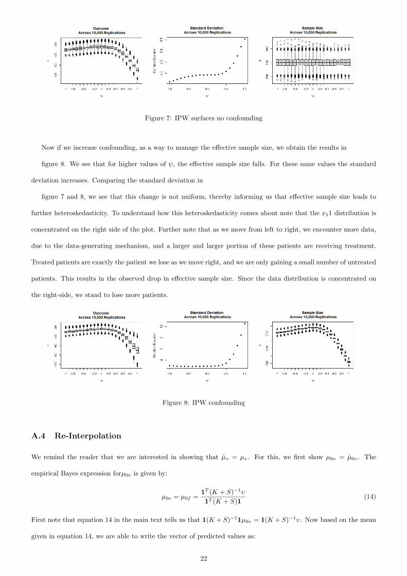
Figure 7: IPW surfaces no confounding
Now if we increase confounding, as a way to manage the effective sample size, we obtain the results in
figure 8. We see that for higher values of ψ, the effective sample size falls. For these same values the standard
deviation increases. Comparing the standard deviation in
figure 7 and 8, we see that this change is not uniform, thereby informing us that effective sample size leads to
further heteroskedasticity. To understand how this heteroskedasticity comes about note that the x11 distribution is
concentrated on the right side of the plot. Further note that as we move from left to right, we encounter more data,
due to the data-generating mechanism, and a larger and larger portion of these patients are receiving treatment.
Treated patients are exactly the patient we lose as we move right, and we are only gaining a small number of untreated
patients. This results in the observed drop in effective sample size. Since the data distribution is concentrated on
the right-side, we stand to lose more patients.
Figure 8: IPW confounding
A.4 Re-Interpolation
We remind the reader that we are interested in showing that µυ = µυ. For this, we first show µ0υ = µ0υ. The
empirical Bayes expression forµ0v is given by:
µ0v = µ0f =1T (K + S)−1υ
1T (K + S)1(14)
First note that equation 14 in the main text tells us that 1(K + S)−11µ0υ = 1(K + S)−1υ. Now based on the mean
given in equation 14, we are able to write the vector of predicted values as:
22

υ = 1µ0v +K(K + S)−1(υ − 1µ0v) (15)
Then substituting this into the expression for µ0υ, analogous to expression 14, we obtain:
µ0υ =1TK−1υ
1TK1
=1K−11µ0υ + 1(K + S)−1(υ − 1µ0f )
1K−11
=µ0υ +1(K + S)−1υ − 1(K + S)−11µ0υ
1K−11
=µ0υ + 0
(16)
Consequently plugging in the expression for υ into the expression for the posterior mean in the reinterpolation model
we get
µυ = µ0υ + kTK(v − 1µ0υ)
= µ0υ + kTK−1(1µ0y +K(K + S)−1(y − 1µ0f )− 1µ0υ)
= µ0υ + kTK−11µ0υ + kT (K + S)−1(y − 1µ0f )− kTK−11µ0υ)
= µ0v + kT (K + S)−1(υ − 1µ0υ)
= µυ
(17)
Then, the Kriging variance at a new sample point is σ2υ(ψ) = k(ψ,ψ)− kTK−1k and it has the desired property
of having zero error at already sampled points. We remind the reader that, although we have not been explicit about
it in the notation, the posterior mean also depends on ψ, as µυ(ψ). This allows us to use the expected improvement
with all its usual features.
B Appendix B: Simulations
B.1 Identification of Locally Optimal Regimes
We may ask how to identify the optimal DTR in a family of regimes treat if x1 > ψ for a data-generating mechanism
with Y = 1000(−x1 + (x1 + 0.5)(x1 − 0.5)z1), and x1 ∼ U(−1.5, 1.5). Plotting the graph of g(x)f(x) as defined in
the main text and further evaluating the integral in order to obtain the value function for regimes in the family we
obtain the following plots:
23
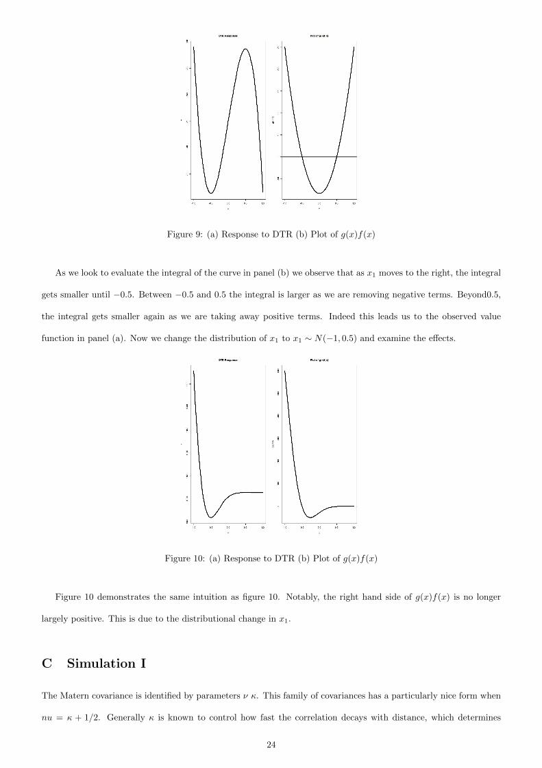
Figure 9: (a) Response to DTR (b) Plot of g(x)f(x)
As we look to evaluate the integral of the curve in panel (b) we observe that as x1 moves to the right, the integral
gets smaller until −0.5. Between −0.5 and 0.5 the integral is larger as we are removing negative terms. Beyond0.5,
the integral gets smaller again as we are taking away positive terms. Indeed this leads us to the observed value
function in panel (a). Now we change the distribution of x1 to x1 ∼ N(−1, 0.5) and examine the effects.
Figure 10: (a) Response to DTR (b) Plot of g(x)f(x)
Figure 10 demonstrates the same intuition as figure 10. Notably, the right hand side of g(x)f(x) is no longer
largely positive. This is due to the distributional change in x1.
C Simulation I
The Matern covariance is identified by parameters ν κ. This family of covariances has a particularly nice form when
nu = κ + 1/2. Generally κ is known to control how fast the correlation decays with distance, which determines
24

the low frequency (Coarse-scale) behaviour. ν is known to control the high frequency (fine-scale) smoothness of the
sample paths.
In this section of the appendix, we explore a variety of different simulations settings.
C.1 Matern 3/2 Covariance
We first change the covariance from Matern 5/2 to Matern 3/2. In figure 11, we observe the visited points in the
EGO algorithm, across 150 replicates. As expected, the algorithm spends more time around the true optimum of
0.9 for the homoskedastic and heteroskedastic approaches.
Figure 11: Sampled Points for Matern 3/2 Covariance (a) Interpolating (b) Homoskedastic (c) Heteroskedastic
We now examine the same type of results as in the main paper, but with this different covariance function. We
note that the results are pretty similar. This is positive in some ways as it emphasizes that the results are robust to
modeling decisions.
Table 6: Optimal threshold ψ for Matern 3/2 covariance, with constant mean (Known optimizer: 0.9). Grid search
minimizer: 0.255 (0.84).
Mean (SD) +1 Point +5 Points +10 Points +15 Points +20 Points +25 Points Number Converge
Interpolating 0.63 (0.622) 0.639 (0.617) 0.659 (0.593) 0.655 (0.597) 0.606 (0.641) 0.549 (0.694) 149
Homoskedastic 0.688 (0.556) 0.792 (0.387) 0.817 (0.345) 0.823 (0.334) 0.834 (0.31) 0.849 (0.29) 150
Heteroskedastic 0.697 (0.538) 0.738 (0.5) 0.831 (0.316) 0.829 (0.314) 0.842 (0.289) 0.833 (0.322) 150
Table 7: Optimal threshold ψ for Matern 3/2 covariance, with constant mean (Known optimizer: 0.9). Grid search
minimizer: 0.83 (1.68).
Median (IQR) +1 Point +5 Points +10 Points +15 Points +20 Points +25 Points Number Converge
Interpolating 0.857 (0.134) 0.857 (0.15) 0.87 (0.125) 0.87 (0.124) 0.857 (0.128) 0.857 (0.158) 149
Homoskedastic 0.857 (0.081) 0.886 (0.102) 0.883 (0.091) 0.887 (0.095) 0.885 (0.09) 0.892 (0.089) 150
Heteroskedastic 0.857 (0.08) 0.882 (0.082) 0.886 (0.091) 0.884 (0.084) 0.891 (0.094) 0.889 (0.095) 150
25

Table 8: Value at optimal threshold ψ for Matern 3/2 covariance, with constant mean (Known value: -0.1649). Grid
search value: -0.177 (0.015).
Mean (SD) +1 Point +5 Points +10 Points +15 Points +20 Points +25 Points Number Converge
Interpolating -0.169 (0.015) -0.172 (0.015) -0.173 (0.015) -0.173 (0.015) -0.174 (0.015) -0.174 (0.015) 149
Homoskedastic -0.167 (0.015) -0.167 (0.015) -0.167 (0.015) -0.167 (0.015) -0.167 (0.015) -0.167 (0.015) 150
Heteroskedastic -0.168 (0.015) -0.167 (0.014) -0.167 (0.014) -0.167 (0.014) -0.167 (0.014) -0.167 (0.014) 150
Table 9: Value at optimal threshold ψ for Matern 3/2 covariance, with constant mean (Known value: -0.1649). Grid
search value: -0.176 (0.021) ) .
Median (IQR) +1 Point +5 Points +10 Points +15 Points +20 Points +25 Points Number Converge
Interpolating -0.17 (0.019) -0.171 (0.022) -0.172 (0.02) -0.172 (0.02) -0.173 (0.021) -0.173 (0.021) 149
Homoskedastic -0.168 (0.019) -0.166 (0.019) -0.167 (0.019) -0.167 (0.019) -0.167 (0.018) -0.167 (0.017) 150
Heteroskedastic -0.167 (0.019) -0.167 (0.019) -0.167 (0.018) -0.167 (0.019) -0.167 (0.019) -0.167 (0.019) 150
Table 10: Coverage probability for 95% confidence interval across 150 replications
+5 Points +25 Points
Interpolating 0.92 0.99
Homoskedastic 0.93 0.95
Heterosekdastic 0.84 0.84
Figure 12: Optimal Threshold
26

Figure 13: Optimal Value
C.2 Log Normal Prior on θ
In this section, we place a Log-Normal prior on the covariance parameters θ. We have already discussed that this
approach is not necessarily very coherent with the heteroskedastic approach. Now, to calibrate this prior, we select
the mean and variance parameters for the prior such that for an increment that is 10% of the range of ψ values, θ
has 95th and 5th percent quantiles corresponding to a correlation between approximately 0 and 0.95.
We note that though the results are pretty much the same, models in all replications converged. This is similar
to what Lizotte [2008] has observed: that this prior has a stabilizing effect on the parameter estimation process of
these models
Table 11: Optimal threshold ψ for Matern 5/2 covariance, with constant mean (Known optimizer: 0.9). Grid search
minimizer: 0.26 (0.838).
Mean (SD) +1 Point +5 Points +10 Points +15 Points +20 Points +25 Points Number Converge
Interpolating 0.614 (0.629) 0.624 (0.608) 0.596 (0.64) 0.57 (0.655) 0.571 (0.657) 0.548 (0.679) 150
Homoskedastic 0.713 (0.524) 0.791 (0.417) 0.802 (0.382) 0.767 (0.45) 0.743 (0.487) 0.768 (0.456) 150
Heteroskedastic 0.703 (0.534) 0.777 (0.445) 0.775 (0.43) 0.737 (0.495) 0.752 (0.483) 0.789 (0.418) 150
27
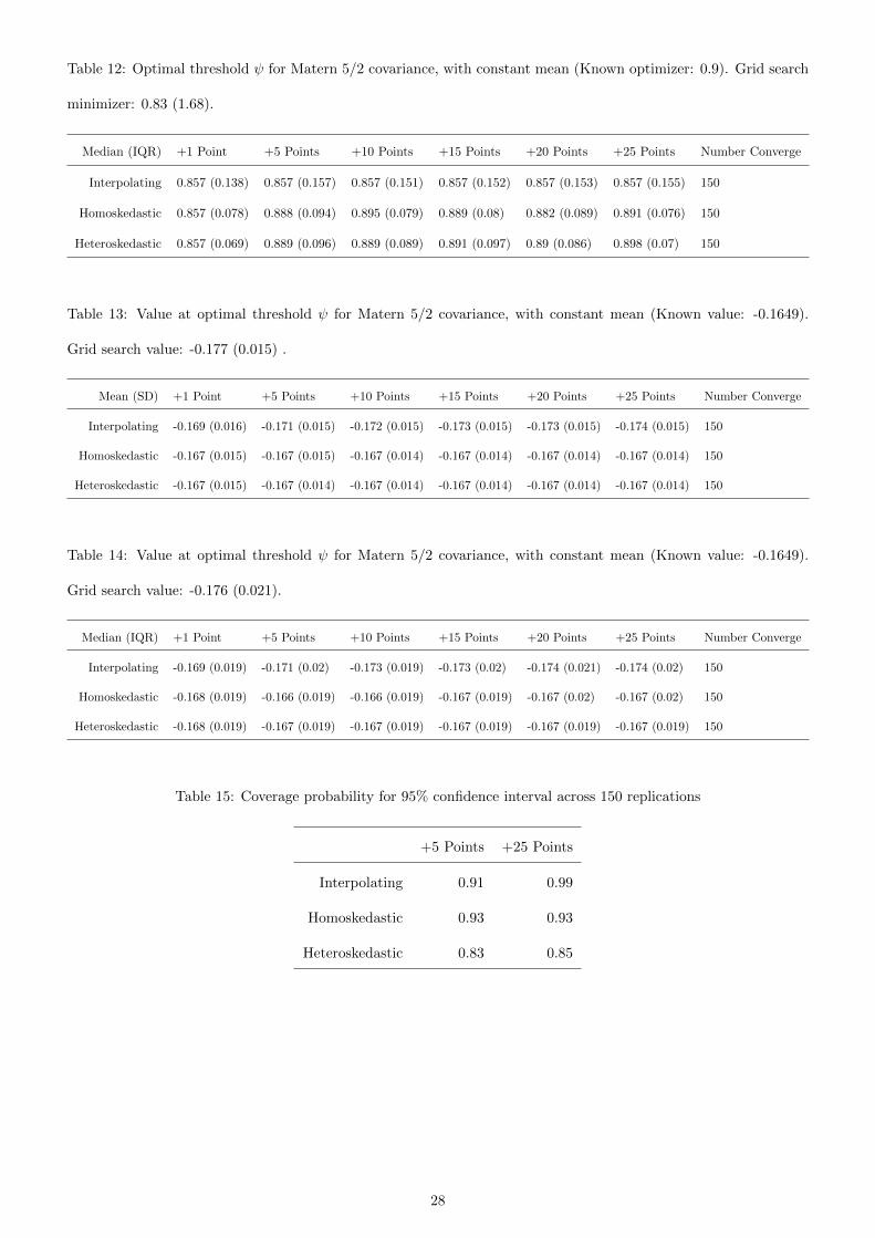
Table 12: Optimal threshold ψ for Matern 5/2 covariance, with constant mean (Known optimizer: 0.9). Grid search
minimizer: 0.83 (1.68).
Median (IQR) +1 Point +5 Points +10 Points +15 Points +20 Points +25 Points Number Converge
Interpolating 0.857 (0.138) 0.857 (0.157) 0.857 (0.151) 0.857 (0.152) 0.857 (0.153) 0.857 (0.155) 150
Homoskedastic 0.857 (0.078) 0.888 (0.094) 0.895 (0.079) 0.889 (0.08) 0.882 (0.089) 0.891 (0.076) 150
Heteroskedastic 0.857 (0.069) 0.889 (0.096) 0.889 (0.089) 0.891 (0.097) 0.89 (0.086) 0.898 (0.07) 150
Table 13: Value at optimal threshold ψ for Matern 5/2 covariance, with constant mean (Known value: -0.1649).
Grid search value: -0.177 (0.015) .
Mean (SD) +1 Point +5 Points +10 Points +15 Points +20 Points +25 Points Number Converge
Interpolating -0.169 (0.016) -0.171 (0.015) -0.172 (0.015) -0.173 (0.015) -0.173 (0.015) -0.174 (0.015) 150
Homoskedastic -0.167 (0.015) -0.167 (0.015) -0.167 (0.014) -0.167 (0.014) -0.167 (0.014) -0.167 (0.014) 150
Heteroskedastic -0.167 (0.015) -0.167 (0.014) -0.167 (0.014) -0.167 (0.014) -0.167 (0.014) -0.167 (0.014) 150
Table 14: Value at optimal threshold ψ for Matern 5/2 covariance, with constant mean (Known value: -0.1649).
Grid search value: -0.176 (0.021).
Median (IQR) +1 Point +5 Points +10 Points +15 Points +20 Points +25 Points Number Converge
Interpolating -0.169 (0.019) -0.171 (0.02) -0.173 (0.019) -0.173 (0.02) -0.174 (0.021) -0.174 (0.02) 150
Homoskedastic -0.168 (0.019) -0.166 (0.019) -0.166 (0.019) -0.167 (0.019) -0.167 (0.02) -0.167 (0.02) 150
Heteroskedastic -0.168 (0.019) -0.167 (0.019) -0.167 (0.019) -0.167 (0.019) -0.167 (0.019) -0.167 (0.019) 150
Table 15: Coverage probability for 95% confidence interval across 150 replications
+5 Points +25 Points
Interpolating 0.91 0.99
Homoskedastic 0.93 0.93
Heteroskedastic 0.83 0.85
28

Figure 14: Optimal Threshold
Figure 15: Optimal Value
C.3 Sample Size (n=500)
We further investigate the case of a smaller sample size. We observe that again the homoskedastic and heteroskedastic
approaches work well, though there is slightly more variability in the optimum than for the larger sample size case.
This is expected. We note that the grid search performs even worse.
29

Table 16: Optimal threshold ψ for Matern 5/2 covariance, with constant mean (Known optimizer: 0.9). Grid search
minimizer: -0.11 (0.882) .
Mean (SD) +1 Point +5 Points +10 Points +15 Points +20 Points +25 Points Number Converge
Interpolating 0.313 (0.813) 0.344 (0.809) 0.323 (0.816) 0.36 (0.8) 0.329 (0.815) 0.336 (0.823) 140
Homoskedastic 0.547 (0.69) 0.6 (0.672) 0.641 (0.651) 0.648 (0.622) 0.673 (0.596) 0.682 (0.579) 150
Heteroskedastic 0.453 (0.752) 0.576 (0.682) 0.623 (0.657) 0.615 (0.657) 0.627 (0.632) 0.597 (0.663) 138
Table 17: Optimal threshold ψ for Matern 5/2 covariance, with constant mean (Known optimizer: 0.9). Grid search
minimizer: -0.71 (1.728) .
Median (IQR) +1 Point +5 Points +10 Points +15 Points +20 Points +25 Points Number Converge
Interpolating 0.857 (1.5) 0.857 (1.623) 0.849 (1.684) 0.852 (1.582) 0.838 (1.686) 0.844 (1.688) 140
Homoskedastic 0.857 (0.156) 0.894 (0.142) 0.897 (0.105) 0.893 (0.102) 0.893 (0.09) 0.89 (0.104) 150
Heteroskedastic 0.857 (1.566) 0.878 (0.158) 0.899 (0.131) 0.895 (0.117) 0.895 (0.105) 0.894 (0.132) 138
Table 18: Value at optimal threshold ψ for Matern 5/2 covariance, with constant mean (Known value: -0.1649).
Grid search value: -0.185 (0.02) .
Mean (SD) +1 Point +5 Points +10 Points +15 Points +20 Points +25 Points Number Converge
Interpolating -0.174 (0.023) -0.176 (0.023) -0.177 (0.024) -0.178 (0.023) -0.179 (0.023) -0.18 (0.023) 140
Homoskedastic -0.169 (0.022) -0.168 (0.022) -0.168 (0.021) -0.168 (0.021) -0.168 (0.021) -0.168 (0.021) 150
Heteroskedastic -0.168 (0.021) -0.167 (0.02) -0.167 (0.021) -0.167 (0.02) -0.166 (0.02) -0.167 (0.02) 138
Table 19: Value at optimal threshold ψ for Matern 5/2 covariance, with constant mean (Known value: -0.1649).
Grid search value: -0.186 (0.029) .
Median (IQR) Points 1 Points 5 Points 10 Points 15 Points 20 Points 25 Number Converge
Interpolating -0.173 (0.034) -0.176 (0.034) -0.177 (0.034) -0.177 (0.033) -0.178 (0.034) -0.179 (0.033) 140
Homoskedastic -0.169 (0.033) -0.168 (0.03) -0.168 (0.03) -0.169 (0.03) -0.168 (0.031) -0.168 (0.03) 150
Heteroskedastic -0.169 (0.029) -0.167 (0.028) -0.168 (0.029) -0.168 (0.029) -0.168 (0.029) -0.167 (0.029) 138
30

Table 20: Coverage probability for 95% confidence interval for 95% confidence interval
+5 Points +25 Points
Interpolating 0.89 0.99
Homoskedastic 0.88 0.91
Heteroskedastic 0.81 0.80
Figure 16: Optimal Threshold
Figure 17: Optimal Value
31

References
Bruce Ankenman, Barry L Nelson, and Jeremy Staum. Stochastic kriging for simulation metamodeling. In 2008
Winter Simulation Conference, pages 362–370. IEEE, 2008.
Elja Arjas and Olli Saarela. Optimal dynamic regimes: Presenting a case for predictive inference. The International
Journal of Biostatistics, 6(2), 2010.
Carla Currin, Toby Mitchell, Max Morris, and Don Ylvisaker. Bayesian prediction of deterministic functions, with
applications to the design and analysis of computer experiments. Journal of the American Statistical Association,
86(416):953–963, 1991.
George J Davis and Max D Morris. Six factors which affect the condition number of matrices associated with kriging.
Mathematical Geology, 29(5):669–683, 1997.
Alexander IJ Forrester, Andy J Keane, and Neil W Bressloff. Design and analysis of ”noisy” computer experiments.
AIAA Journal, 44(10):2331–2339, 2006.
Peter Frazier, Warren Powell, and Savas Dayanik. The knowledge-gradient policy for correlated normal beliefs.
INFORMS Journal on Computing, 21(4):599–613, 2009.
Peter I Frazier and Jialei Wang. Bayesian optimization for materials design. In Information Science for Materials
Discovery and Design, pages 45–75. Springer, 2016.
Peter I Frazier, Jing Xie, and Stephen E Chick. Value of information methods for pairwise sampling with correlations.
In Proceedings of the 2011 Winter Simulation Conference (WSC), pages 3974–3986. IEEE, 2011.
Paul W Goldberg, Christopher KI Williams, and Christopher M Bishop. Regression with input-dependent noise: A
Gaussian process treatment. Advances in Neural Information Processing Systems, 10:493–499, 1997.
Deng Huang, Theodore T Allen, William I Notz, and Ning Zeng. Global optimization of stochastic black-box systems
via sequential kriging meta-models. Journal of Global Optimization, 34(3):441–466, 2006.
Hamed Jalali, Inneke Van Nieuwenhuyse, and Victor Picheny. Comparison of kriging-based algorithms for simulation
optimization with heterogeneous noise. European Journal of Operational Research, 261(1):279–301, 2017.
Donald R Jones, Matthias Schonlau, and William J Welch. Efficient global optimization of expensive black-box
functions. Journal of Global Optimization, 13(4):455–492, 1998.
Kristian Kersting, Christian Plagemann, Patrick Pfaff, and Wolfram Burgard. Most likely heteroscedastic Gaussian
process regression. In Proceedings of the 24th International Conference on Machine learning, pages 393–400, 2007.
32

Daniel James Lizotte. Practical Bayesian Optimization. PhD thesis, University of Alberta, Edmonton, Alta., Canada,
2008.
Marco Locatelli. Bayesian algorithms for one-dimensional global optimization. Journal of Global Optimization, 10
(1):57–76, 1997.
Jay D Martin and Timothy W Simpson. Use of kriging models to approximate deterministic computer models. AIAA
Journal, 43(4):853–863, 2005.
Thomas A Murray, Ying Yuan, and Peter F Thall. A Bayesian machine learning approach for optimizing dynamic
treatment regimes. Journal of the American Statistical Association, 113(523):1255–1267, 2018.
Anthony O’Hagan, JM Bernardo, JO Berger, AP Dawid, and Smith. Uncertainty analysis and other inference tools
for complex computer codes. Bayesian Statistics, 6:503–524, 1999.
Liliana Orellana, Andrea Rotnitzky, and James M Robins. Dynamic regime marginal structural mean models for
estimation of optimal dynamic treatment regimes, part I: Main content. The International Journal of Biostatistics,
6(2), 2010.
Jeong-Soo Park and Jangsun Baek. Efficient computation of maximum likelihood estimators in a spatial linear model
with power exponential covariogram. Computers & Geosciences, 27(1):1–7, 2001.
Victor Picheny and David Ginsbourger. Noisy kriging-based optimization methods: a unified implementation within
the diceoptim package. Computational Statistics & Data Analysis, 71:1035–1053, 2014.
Victor Picheny, Tobias Wagner, and David Ginsbourger. A benchmark of kriging-based infill criteria for noisy
optimization. Structural and Multidisciplinary Optimization, 48(3):607–626, 2013.
James Robins. A new approach to causal inference in mortality studies with a sustained exposure period—application
to control of the healthy worker survivor effect. Mathematical Modelling, 7(9-12):1393–1512, 1986.
Daniel Rodriguez Duque, David A Stephens, Erica EM Moodie, and Marina B Klein. Semi-parametric Bayesian
inference for dynamic treatment regimes via dynamic regime marginal structural models. 2021.
Olivier Roustant, David Ginsbourger, and Yves Deville. Dicekriging, diceoptim: Two R packages for the analysis of
computer experiments by kriging-based metamodelling and optimization. Journal of Statistical Software, 51(1):
54p, 2012.
Olli Saarela, David A Stephens, Erica EM Moodie, and Marina B Klein. On Bayesian estimation of marginal
structural models. Biometrics, 71(2):279–288, 2015.
33

Jerome Sacks, William J Welch, Toby J Mitchell, and Henry P Wynn. Design and analysis of computer experiments.
Statistical Science, pages 409–423, 1989.
Michael James Sasena. Flexibility and efficiency enhancements for constrained global design optimization with kriging
approximations. PhD thesis, Citeseer, 2002.
Jian Qing Shi and Taeryon Choi. Gaussian process regression analysis for functional data. CRC Press, 2011.
Timothy W Simpson, Jonathan RA Maier, and Farrokh Mistree. A product platform concept exploration
method for product family design. In ASME Design Theory and Methodology, volume 9, pages 1–219. ASME,
ASMEDETC99/DTM, 1999.
Michael L Stein. Interpolation of spatial data: some theory for kriging. Springer Science & Business Media, 2012.
Chunyi Wang. Gaussian process regression with heteroscedastic residuals and fast MCMC methods. PhD thesis, 2014.
Yanxun Xu, Peter Muller, Abdus S Wahed, and Peter F Thall. Bayesian nonparametric estimation for dynamic
treatment regimes with sequential transition times. Journal of the American Statistical Association, 111(515):
921–950, 2016.
Jun Yin, Szu Hui Ng, and Kien Ming Ng. Kriging metamodel with modified nugget-effect: The heteroscedastic
variance case. Computers & Industrial Engineering, 61(3):760–777, 2011.
Qiu-Hu Zhang and Yi-Qing Ni. Improved most likely heteroscedastic Gaussian process regression via bayesian residual
moment estimator. IEEE Transactions on Signal Processing, 68:3450–3460, 2020.
Yingqi Zhao, Donglin Zeng, John Rush, and Michael Kosorok. Estimating individualized treatment rules using
outcome weighted learning. Journal of the American Statistical Association, 107(499):1106–1118, 2012.
Yufan Zhao, Michael R Kosorok, and Donglin Zeng. Reinforcement learning design for cancer clinical trials. Statistics
in Medicine, 28(26):3294–3315, 2009.
34