Universidade do Minho

Escola de Engenharia

Departamento de Inform

´

atica

Daniel Ara´ujo

Real-Time Intelligence

June 2016

Universidade do Minho

Escola de Engenharia

Departamento de Inform

´

atica

Daniel Ara´ujo

Real-Time Intelligence

Master dissertation

Master Degree in Computer Science

Dissertation supervised by

Paulo Novais - Universidade do Minho

Andr

´

e Ribeiro - Performetric

June 2016

A C K N O W L E D G E M E N T S

Firstly and foremost, I would like to express my gratitude to my parents and my brother,for their support, they have always helped me to think more clearly, and without them thiswork would not have been possible.

I would also like to thank to my friends at Performetric, particularly to Andre Pimenta(co-supervisor), who was available at all times to provide technical guidance and friendship.

Last but not least, I would like to thank to Professor Paulo Novais for the supervision ofthis work and the motivation he provided.

i

A B S T R A C T

Over the past 20 years, data has increased in a large scale in various fields. This explosiveincrease of global data led to the coin of the term Big Data. Big data is mainly used to des-cribe enormous datasets that typically includes masses of unstructured data that may needreal-time analysis. This paradigm brings important challenges on tasks like data acquisi-tion, storage and analysis. The ability to perform these tasks efficiently got the attentionof researchers as it brings a lot of oportunities for creating new value. Another topic withgrowing importance is the usage of biometrics, that have been used in a wide set of appli-cation areas as, for example, healthcare and security. In this work it is intended to handlethe data pipeline of data generated by a large scale biometrics application providing basisfor real-time analytics and behavioural classification. The challenges regarding analyticalqueries (with real-time requirements, due to the need of monitoring the metrics/behavior)and classifiers’ training are particularly addressed.

Key Words: Real-Time Analytics, Big Data, NoSQL Databases, Machine Learning, Bio-metrics, Mouse Dynamics

ii

R E S U M O

Nos os ultimos 20 anos, a quantidade de dados armazenados e passıveis de serem proces-sados, tem vindo a aumentar em areas bastante diversas. Este aumento explosivo, aliadoas potencialidades que surgem como consequencia do mesmo, levou ao aparecimento dotermo Big Data. Big Data abrange essencialmente grandes volumes de dados, possivelmentecom pouca estrutura e com necessidade de processamento em tempo real. As especificida-des apresentadas levaram ao apareciemento de desafios nas diversas tarefas do pipelinetıpico de processamento de dados como, por exemplo, a aquisicao, armazenamento e aanalise. A capacidade de realizar estas tarefas de uma forma eficiente tem sido alvo de es-tudo tanto pela industria como pela comunidade academica, abrindo portas para a criacaode valor. Uma outra area onde a evolucao tem sido notoria e a utilizacao de biometicas com-portamentais que tem vindo a ser cada vez mais acentuada em diferentes cenarios como,por exemplo, na area dos cuidados de saude ou na seguranca. Neste trabalho um dos ob-jetivos passa pela gestao do pipeline de processamento de dados de uma aplicacao de largaescala, na area das biometricas comportamentais, de forma a possibilitar a obtencao demetricas em tempo real sobre os dados (viabilizando a sua monitorizacao) e a classificacaoautomatica de registos sobre fadiga na interacao homem-maquina (em larga escala).

Palavras-chave: Indicadores em tempo real, Big Data, Bases de dados NoSQL, MachineLearning, Biometricas Comportamentais

iii

C O N T E N T S

1 introduction 2

1.1 Motivation 2

1.1.1 Big Data 2

1.1.2 Real-Time Analytics 3

1.2 Context 4

1.3 Objectives 4

1.4 Methodology 5

1.5 Work Plan 5

1.6 Document Structure 5

2 state of the art 8

2.1 Data Generation and Data Acquisition 8

2.1.1 Data Collection 10

2.1.2 Data Pre-processing 11

2.2 Data Storage 11

2.2.1 Cloud Computing 12

2.2.2 Distributed File Systems 12

2.2.3 CAP Theorem 13

2.2.4 NoSQL - Not only SQL 14

2.3 Data Analytics 20

2.3.1 MapReduce 21

2.3.2 Real Time Analytics 23

2.3.3 MongoDB Aggregation Framework 24

2.4 Machine Learning 25

2.4.1 Introduction to Learning 25

2.4.2 Deep Neural Network Architecutres 28

2.4.3 Popular Frameworks and Libraries 30

2.5 Related Projects 31

2.5.1 Financial Services - MetLife 31

2.5.2 Government - The City of Chicago 31

2.5.3 High Tech - Expedia 32

2.5.4 Retail - Otto 32

2.6 Summary 32

3 the problem and its challenges 34

3.1 System Architecture 36

iv

Contents

3.1.1 Data Model 36

3.1.2 System Components 38

3.1.3 Deployment View 39

3.2 Rate of Data Generation and Growth Projection 40

3.2.1 Data Analytics 41

3.2.2 Data Insertion 42

3.2.3 Classifier Training 43

3.3 Summary 44

4 case studies 45

4.1 Experimental setup and Enhancements Discussion 45

4.1.1 MongoDB Aggregation Framework 45

4.1.2 Caching the queries’ results with EhCache 50

4.1.3 H2O Package 51

4.2 Testing Setup 53

4.2.1 Physical Setup 53

4.2.2 Data Collection 54

4.3 Results 57

4.3.1 Data Aggregation 58

4.3.2 Data Classification 63

4.4 Summary 65

5 result analysis and discussion 66

5.1 Data Aggregation 66

5.1.1 Simple queries results analysis 66

5.1.2 Complex queries results analysis 67

5.1.3 Caching queries results analysis 67

5.2 Data Classification 68

5.3 Project Execution Overview 69

6 conclusion 70

6.1 Work Synthesis 70

6.2 Prospect for future work 71

a queries response times 78

a.1 Company Queries Execution Performance 78

a.2 Team Queries Execution Performance 79

a.3 User Queries Execution Performance 81

a.4 Group By Queries Execution Performance 82

a.5 Hourly Queries Execution Performance 84

a.6 Cache Performance 87

v

L I S T O F F I G U R E S

Figure 1 Work plan showing the timeline of the set of tasks in this disserta-tion. 6

Figure 2 The Big Data analysis Pipeline according to Bertino et al. (2011). 9

Figure 3 HDFS Architecture from https://hadoop.apache.org/docs/r1.2.

1/hdfs_design.html. 13

Figure 4 Mapping between Big Data 3 V’s and NoSQL System features. 14

Figure 5 Classification of popular DBMSs according to the CAP theorem. 15

Figure 6 Hadoop MapReduce architecture. 22

Figure 7 Pseudocode representing a words counting implementation in map-reduce. 22

Figure 8 MongoDB Aggregation Pipeline example. 25

Figure 9 Bias and variance in dart-throwing (Domingos (2012)). 28

Figure 10 Functional model of an artificial neural network (Rojas (2013)). 29

Figure 11 Overview of the concepts presented in chapter 2. 33

Figure 12 Conceptual Diagram of the Data Model (according to Chen (1976)). 37

Figure 13 The deplyment view (showing the layered architecture). 38

Figure 14 The deployment view (showing the devices that take part in the sys-tem). 40

Figure 15 A representation of a sharded deployment in MongoDB. 43

Figure 16 Example of an aggregation pipeline (includes 2 stages). 47

Figure 17 Example of an aggregation pipeline (includes 3 stages). 48

Figure 18 Pseudocode representing the implementation of a simple MongoDBquery. 48

Figure 19 Pseudocode representing the implementation of a MongoDB aggre-gation framework query. 49

Figure 20 Pseudocode representing the implementation of the case operator. 50

Figure 21 Example of usage of the defined cache (Java code). 51

Figure 22 Example of usage of neural networks with H2O (R code). 52

Figure 23 MongoDB replica set topology. 53

Figure 24 MongoDB replica set topology (after primary member becomes un-available). 54

Figure 25 Example of JMH usage (Java code). 55

Figure 26 Example of output generated by JMH benchmarks. 56

vi

List of Figures

Figure 27 Piece of AWK code used for parsing the output generated by JMH. 57

Figure 28 Comparison between Java and MongoDB aggregation frameworkimplementations (queries about a specific company name) for a cur-rent time interval (see subsection 3.2.1). 59

Figure 29 Comparison between Java and MongoDB aggregation frameworkimplementations (queries about a specific company name) for a pasttime interval (see subsection 3.2.1). 59

Figure 30 Comparison between Java and MongoDB aggregation frameworkimplementations (queries about a specific team name) for a currenttime interval (see subsection 3.2.1). 60

Figure 31 Comparison between Java and MongoDB aggregation frameworkimplementations (queries about a specific team name) for a past timeinterval (see subsection 3.2.1). 60

Figure 32 Comparison between Java and MongoDB aggregation frameworkimplementations (queries about a specific user name) for a currenttime interval (see subsection 3.2.1). 61

Figure 33 Comparison between Java and MongoDB aggregation frameworkimplementations (queries about a specific user name) for a past timeinterval (see subsection 3.2.1). 61

Figure 34 Comparison between Java and MongoDB aggregation frameworkimplementations (queries about a specific company name). 62

Figure 35 Comparison between Java and MongoDB aggregation frameworkimplementations (queries about a specific team name). 62

Figure 36 Comparison between Java and MongoDB aggregation frameworkimplementations (queries about a specific user name). 63

Figure 37 Comparison between previous and MongoDB aggregation frame-work implementations (query about data generated in the currenthour). 85

Figure 38 Comparison between previous and MongoDB aggregation frame-work implementations (query about data generated in the last hour). 86

vii

L I S T O F TA B L E S

Table 1 NoSQL DBMS comparison. 19

Table 2 Data growth projections. 40

Table 3 Data growth projections. 42

Table 4 Classifier training results. 64

Table 5 Throughput of a set of queries where data is filtered by companyname (Java implementation). 78

Table 6 Throughput of a set of queries where data is filtered by companyname (MongoDB Agg. implementation). 78

Table 7 Average time of a set of queries where data is filtered by companyname (Java implementation). 79

Table 8 Average time of a set of queries where data is filtered by companyname (MongoDB Agg. implementation). 79

Table 9 Throughput of a set of queries where data is filtered by group name(Java implementation). 79

Table 10 Throughput of a set of queries where data is filtered by group name(MongoDB Agg. implementation). 80

Table 11 Average of a set of queries where data is filtered by group name (Javaimplementation). 80

Table 12 Average of a set of queries where data is filtered by group name(MongoDB Agg. implementation). 80

Table 13 Throughput of a set of queries where data is filtered by user name(Java implementation). 81

Table 14 Throughput of a set of queries where data is filtered by companyname (MongoDB Agg. implementation). 81

Table 15 Average time of a set of queries where data is filtered by companyname (Java implementation). 81

Table 16 Average time of a set of queries where data is filtered by companyname (MongoDB Agg. implementation). 82

Table 17 Throughput of a set of queries where data is grouped by time inter-vals according to labels (Java implementation). 82

Table 18 Throughput of a set of queries where data is grouped by time inter-vals according to labels (MongoDB Agg. implementation). 83

viii

List of Tables

Table 19 Average times of a set of queries where data is grouped by timeintervals according to labels (Java implementation). 83

Table 20 Average times of a set of queries where data is grouped by timeintervals according to labels (MongoDB Agg. implementation). 84

Table 21 Throughput of a set of queries where the retrived data is from last 2

hours (Java implementation). 84

Table 22 Throughput of a set of queries where the retrived data is from last 2

hours (MongoDB Agg. implementation). 84

Table 23 Average time of a set of queries where the retrived data is from last2 hours (Java implementation). 85

Table 24 Average time of a set of queries where the retrived data is from last2 hours (MongoDB Agg. implementation). 85

Table 25 Throughput of the set of queries using the Cache system. 87

Table 26 Average time of the set of queries using the Cache system. 88

ix

L I S T O F A B B R E V I AT I O N S

ACID Atomicity, Consistency, Isolation, Durability

ANN Artificial Neural Network

API Application Programming Interface

BASE Basically available, Soft state, Eventual consistency

BSON Binary JSON

CAP Consistency, Availability, Partition tolerance

CRUD Create, Read, Update, Delete

DBMS Data Base Management System

DFS Distributed File System

ETA Estimated Time of Arrival

ETL Extract, Transform, Load

GLM Generalized Linear Mode

GPS Global Positioning System

HTTP Hypertext Transfer Protocol

IaaS Infrastructure as a Service

JDK Java SE Development Kit

JMH Java Microbenchmark Harness

JSON JavaScript Object Notation

JVM Java Virtual Machine

KNN K-Nearest Neighbors

MSE Mean Squared Error

NoSQL Not Only SQL

x

List of Tables

PaaS Platform As A Service

PBIAS Percent Bias

RDBMS Relational Database Management System

RMSE Root-Mean-Square Error

SaaS Software As A Service

SQL Structured Query Language

VAR Variance

WSN Wireless Sensor Network

1

1

I N T R O D U C T I O N

1.1 motivation

In recent years, data has increased in a large scale in various fields leading to the coinof the term Big Data, this term has been mainly used to describe enormous datasets thattypically includes masses of unstructured data that may need real-time analysis. As humanbehaviour and personality can be captured through human-computer interaction a massiveopportunity opens for providing wellness services (Carneiro et al. (2008); Pimenta et al.(2014)). Through the use of interaction data, behavioral biometrics (presented, for exemple,in Pimenta et al. (2015)) can be obtained. The usage of biometrics has increased due toseveral factors such as the rise of power and availability of computational power. Oneof the challenges in this kind of approaches has to do with handling the acquired data.The growing volumes, variety and velocity brings challenges in the tasks of pre-processing,storage and providing real-time analytics. In this remaining of this section the conceptsthat were introduced due the mentioned needs are introduced.

1.1.1 Big Data

A large amount of data is created every day by the interactions of billions of people withcomputers, wearable devices, GPS devices, smart phones, and medical devices. In a broadrange of application areas, data is being collected at unprecedented scale Bertino et al.(2011). Not only the volume of data is growing, but also the variety (range of data typesand sources) and velocity (speed of data in and out) of data being collected and stored.These are known as the 3V’s of Big data, enumerated in a research report published byGartner: “Big data is high volume, high velocity, and/or high variety information assetsthat require new forms of processing to enable enhanced decision making, insight discoveryand process optimization” Gartner. In addition to those dimensions, the handling of dataveracity (the biases, noise and abnormalities in data) constitutes the IBM’s 4V’s of Big Data,that give us a good intuition about the term IBM.

2

1.1. Motivation

Despite of its popularity Big Data remains somehow ill-defined, in order to give a bettersense about the term here are two aditional relevant definitions by two of the industryleaders:

MICROSOFT “Big data is the term increasingly used to describe the process of applyingserious computing power - the latest in machine learning and artificial intelligence -to seriously massive and often highly complex sets of information.” Aggarwal (2015)

ORACLE “Big data is the derivation of value from traditional relational database-drivenbusiness decision making, augmented with new sources of unstructured data.” Ag-garwal (2015)

By analysing these large volumes of data, progress can be made. Advances in manyscientific disciplines and enterprise profitability are among the potential beneficial conse-quences of right data usage, and areas like financial services (e.g. algorithmic trading),security (e.g. cybersecurity and fraud detection), healthcare and education are among thetop beneficiaries. In order to do so, challanges related to the 4V’s and also error-handling,privacy issues, and data visualization must be addressed. The data pipeline stages (fromdata acquisition to result interpretation) must be adapted to this new paradigm.

1.1.2 Real-Time Analytics

There is an undergoing transition in the Big Data analytics from being mostly offline (orbatch) to primarily online (real-time) Kejariwal et al. (2015). This trend can be related to theVelocity dimension of the 4 V’s of Big Data: “The high velocity, white-water flow of datafrom innumerable real-time data sources such as market data, Internet of Things, mobile,sensors, clickstream, and even transactions remain largely unnavigated by most firms. Theopportunity to leverage streaming analytics has never been greater.” Gualtieri and Curran(2014).

The term of real-time analytics can have two meanings considering the prespective ofeither the data arriving or the point of view of the end-user. The earlier translates intothe ability of processing data as it arrives, making it possible to aggregate data and extracttrends about the actual situation of the system (streaming analytics). The former refersto the ability to process data with low latency (processing huge amount of data with theresults being available for the end user almost in real-time) making it possible, for example,to to provide recommendations for an user on a website based on its history or to dounpredictable, ad hoc queries against large data sets (online analytics).

Regarding this trend, examples of use cases are mainly related to: visualization of busi-ness metrics in real time, providing highly personalized experiences and acting duringemergencies. These use cases are part of the emerging data-driven society and are used in

3

1.2. Context

various domains such as: social media, health care, internet of things, e-commerce, financialservices, connected vehicles and machine data Pentland (2013); Kejariwal et al. (2015).

1.2 context

This project will be developed in cooperation and under the requirements of Performetric1.Performetric is a company that focuses its activity around the detection of mental fatigue.In order to do so, the developed software uses a set of computer peripherals as sensors.The main goal of the system is to provide a real time analytics platform. The problem thatPerformetric faces relates to the volume, heterogeneity and speed-of-arrival of the data ithas to store and process. Data is generated every 5 minutes for every user, and the numberof users is growing everyday (data volume grows as well). The basic need is the abilityto store and to do data aggregations (in order to calculate the desired metrics) with greatperformance. Another issue that must be tackled is the performance on the training of theclassifier (based on neural networks), since as the data volumes grow bigger and bigger itcan become a bottleneck on the system.

1.3 objectives

The main objective of this project is the development of techniques that enable Performetricsystem the handling of the growing volumes and velocity the generated data. The focus ison problem detection and the experiment and implementation of possible solutions for thegathered contextual needs.

1. To carry an in-depth study on Big Data, in the form a state-of-the-art document.

2. Problem analysis and gathering of the contextual needs, namely the implications ofthe usage of MongoDB as operational data store (and as basis for analytical needs)and the usage of neural networks as classifiers.

3. Design the architecture for a real-time analytics and learning system.

4. Developement of a analytical system that makes it possible to gather indicators inreal-time, by aggregation and learning on large data volumes.

5. Performance tests and result analysis.

1 https://performetric.net

4

1.4. Methodology

1.4 methodology

This dissertation will be developed under an research-action methodology. According tothis methodology, the first step when facing a challenge is to establish a solution hypothesis.Then, takes place the gathering and organization of the relevant pieces of information forthe problem. After that, a proposal of solution will be implemented. The last step consistsin the formulation of the conclusions regarding the obtained results.

Therefore, the project will be developed in the following steps:

• Bibliographic investigation while analysing existing solutions.

• Problem analysis and gathering of organizational context needs.

• Writing the State of the Art document.

• Development of a set of solutions that make it possible to obtain indicators based onexisting data (in real-time).

• Development of a solution that makes it possible to improve the classifer based onexisting data.

• Evaluation of the obtained results.

• Writing the Master’s dissertation.

1.5 work plan

The development of this dissertation evolved through a set of well-defined stages that areshown if the figure 1. It is important to note that there is a constant awareness about theiterative nature of this process that may result in changes of the duration in each stage. Atthis moment, the literature review is complete and the architecture of the system is beingdefined. The work is being performed according to the plan (the kickoff of the project wasat the beginning of October 2015).

1.6 document structure

This document will be divided into 6 chapters where the first chapter, the current one,describes all the motivations for the development of the project and what this project pro-poses to offer at its final stage, as well as, the steps outlined for this process and the type ofresearch that was used as a guideline.

The second chapter describes the analysis made to the state of the art, in which areincluded an overview over the Big Data scene and the current challenges. In each section,

5

1.6. Document Structure

Figure 1.: Work plan showing the timeline of the set of tasks in this dissertation.

there will be an description of the steps of the data pipeline, and relevant findings on eachtopic. The most used tools will be introduced and a comparative analysis will be made,as it will serve as a basis for the following steps of this work. An introduction to the toolMongoDB aswell as a critical analysis is also part of this chapter. The last section providesan overview of Big Data projects on a wide set of areas.

The third chapter introduces the problem. By describing the architecture of the sys-tem through adequated documentation the reasinong about the contextual needs becomessimpler. The gathered needs are then discussed and quantified, the requirements are estab-lished.

In the fourth chapter the improvemetns to the system are discussed and introduced tothe reader. The important and unique aspects of the setup are described. Additionally, thetesting methodology is presented along with the obtained results. Some additional detailsare included in order to give helpful hints to those who work with this or similar systemsin the future.

A careful analysis on the data collected and the results accomplished is made on the fifthchapter. The results are evaluated and compared. The discussion is made around possibleexplanations for the observed results and possible improvements on the testing setup. Inthis chapter valuable conclusions are infered that enable the orientation of data decisionson Performetric.

6

1.6. Document Structure

In the last chapter, it is put together a review of all the work developed and the resultsobtained. Furthermore, the future work that can be done to improve this platform and tobetter validate the results is indicated.

7

2

S TAT E O F T H E A RT

Big Data refers to things one can do at a large scale that cannot be done at a a smaller one:to extract new insights or create new forms of value, in ways that change markets, organi-zations, the relationship between citizens and governments, and more Mayer-Schonbergerand Cukier (2013). Despite still being somewhat an abstract concept it can be clearly saidthat Big Data encomprises the a new generation of technologies and architectures, designedto economically extract value from very large volumes of a wide variety of data, by enablingthe high-velocity capture, discovery and analysis Gantz and Reinsel (2011).

The continuous evolution of Big Data applications has brought advances in architecturesused in the data centers. Sometimes these architectures are unique and have specific solu-tions for storage, networking and computing solutions regarding the particular contextualneeds of the underlying organization. Therefore, when analysing Big Data we should fol-low a top down approach avoiding the risk of losing focus on the initial topic. Hence, thisrevision of the state of the art will be structured acording to the value chain of big dataChen et al. (2014) and its contents will be conditioned by the contextual needs evidencedby Performetric’s system. The value chain of big data can be generally divided into fourphases: data generation, data acquisition, data storage, and data analytics. This approachis similar to the one that is shown it the figure 2 Bertino et al. (2011). Each of the first fourphases of the presented pipeline can be matched with one of the phases of the Big Datavalue chain. For each phase the main concepts, techniques, tools and current challengeswill be introduced and discussed. As it is expressed in the figure 2, there are needs thatare common to all phases these include, but are not limited to: data representation, datacompression (redudancy reduction), data confidentiality and energy management Bertinoet al. (2011); Chen et al. (2014).

2.1 data generation and data acquisition

Data is being generated in a wide set of fields. The main sources are enterprise operationaland trading data, sensor data (Internet of Things), human-computer interaction data anddata generated from scientific research.

8

2.1. Data Generation and Data Acquisition

Figure 2.: The Big Data analysis Pipeline according to Bertino et al. (2011).

Enterprise data is mainly data stored in traditional RDBMSs and it is related to produc-tion, inventory, sales, and financial departments and, in addition to this, there is onlinetrading data. It is estimated that the business data volume of all companies in the worldmay double around every year (1.2 years according to Manyika et al. (2011)). The datasetsthat are a product of scientific applications are also part of the Big Data. Research in areaslike bio-medical applications, computational biology, high-energy physics (for example theLarge Hadron Collider) and behavior analysis (such as in Kandias et al. (2013)) generatesdata at an unprecedented rate.

Sensor applications, commonly known as part of the Internet of things is also a bigsource of data that needs to be processed. Sensors and tiny devices (actuators) embeddedin physical objects—from roadways to pacemakers—are linked through wired and wirelessnetworks, often using the same Internet Protocol (IP) that connects the Internet Chui et al.(2010). Typically, this kind of data may contain redudancy (for example data streams) andhas strong time and space correlation (every data acquisition device are placed at a specificgeographic location and every piece of data has time stamp). The domains of applicationare as diverse as industry Da Xu et al. (2014), agriculture Ruiz-Garcia et al. (2009), trafficGentili and Mirchandani (2012) and medical care Dishongh et al. (2014).

Two important challenges rise regarding data generation, particularly regarding the vol-ume of and the heterogeneity. The first challange is about dealing with the fact that asignificant amount of data is not relevant due to redudancy, and thus having the possibility

9

2.1. Data Generation and Data Acquisition

of being filtered and compressed by orders of magnitude. Defining the filters and beingable to do so online (in order to reduce data sizes from data streams) are the main ques-tions regarding this challenge. The second challenge is to automate the generation of rightmetadata in order to describe what data is recorded and how it is recorded and measuredas the value of data explodes when it can be linked with other data Bertino et al. (2011).

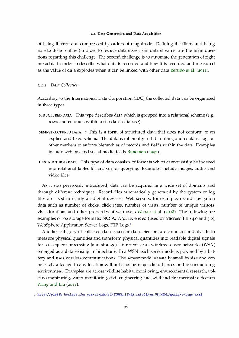
2.1.1 Data Collection

According to the International Data Corporation (IDC) the collected data can be organizedin three types:

STRUCTURED DATA This type describes data which is grouped into a relational scheme (e.g.,rows and columns within a standard database).

SEMI-STRUCTURED DATA : This is a form of structured data that does not conform to anexplicit and fixed schema. The data is inherently self-describing and contains tags orother markers to enforce hierarchies of records and fields within the data. Examplesinclude weblogs and social media feeds Buneman (1997).

UNSTRUCTURED DATA This type of data consists of formats which cannot easily be indexedinto relational tables for analysis or querying. Examples include images, audio andvideo files.

As it was previously introduced, data can be acquired in a wide set of domains andthrough different techniques. Record files automatically generated by the system or logfiles are used in nearly all digital devices. Web servers, for example, record navigationdata such as number of clicks, click rates, number of visits, number of unique visitors,visit durations and other properties of web users Wahab et al. (2008). The following areexamples of log storage formats: NCSA, W3C Extended (used by Microsoft IIS 4.0 and 5.0),WebSphere Application Server Logs, FTP Logs.1

Another category of collected data is sensor data. Sensors are common in daily life tomeasure physical quantities and transform physical quantities into readable digital signalsfor subsequent processing (and storage). In recent years wireless sensor networks (WSN)emerged as a data sensing architechture. In a WSN, each sensor node is powered by a bat-tery and uses wireless communications. The sensor node is usually small in size and canbe easily attached to any location without causing major disturbances on the surroundingenvironment. Examples are across wildlife habitat monitoring, environmental research, vol-cano monitoring, water monitoring, civil engineering and wildland fire forecast/detectionWang and Liu (2011).

1 http://publib.boulder.ibm.com/tividd/td/ITWSA/ITWSA_info45/en_US/HTML/guide/c-logs.html

10

2.2. Data Storage

Methods for acquiring network data such as web crawlers (program used by search en-gines for downloading and storing web pages) are also widely used for data collection.Specialized network monitoring software like Wireshark 2 and SmartSniff 3 are also used inthis context.

2.1.2 Data Pre-processing

In order to improve the data analysis process, a set of techniques should be used. These arepart of the data pre-processing stage and have the objective of dealing with noise in data,redudancy and consistency issues (i.e. data quality). Data integration is a mature researchfield in the database research community. Data warehousing processes, namely ETL (Ex-tract, Transform and Load) are the most used for data integration. Extraction is the processof collecting data (selection and analysis of sources). Transformation is the definition of aseries of data flows that transform and integrate the extracted data into the desired formats.Loading means importing the data resulting from the previous operation into the targetstorage infrastructure. In order to deal with inacurate and incomplete data, data cleaningprocedures may take place. Generally these are associated with the following complemen-tary procedures: defining and determining error types, searching and identifying errors,correcting errors, documenting error examples and error types, and modifying data acqui-sition procedures to reduce future errors Maletic and Marcus (2000). Classic data qualityproblems mainly come from software defects or system misconfiguration. Data redundancymeans an increment of unnecessary data transmission resulting in waste of storage spaceand possibly leads to data inconsistency. Techniques like redundancy detection, data filter-ing, and data compression can be used in order to deal with data redudancy, however itsusage should be carefully weighted as it requires extra processing power.

2.2 data storage

Big data brings more strict requirements on how data is stored and managed. This sectionwill elaborate on the developments in different (technological) fields making big data datapossible. Cloud computing, distributed file systems and NoSQL databases. A comparisionbased on quality attributes of the different NoSQL solutions is hereby presented.

2 https://www.wireshark.org3 http://www.nirsoft.net/utils/smsniff.html

11

2.2. Data Storage

2.2.1 Cloud Computing

The rise of the cloud plays a significant role in big data analytics as it offers the demandedcomputing resources when needed. This translates to a pay for use stategy that enablesthe use of resources on a short-term bases (e.g. more resources on peak hours). Addition-ally there is no need for a upfront commitment about the allocated resources: users canstart small but think big. Improved avalilability is another big advantage of cloud solu-tions. Clouds vary significantly in their specific technologies and implementation, but of-ten provide infrastructure (IaaS), platform (PaaS), and software resources as services (SaaS)Assuncao et al. (2015). Cloud solutions may be private, public or hybrid (additional re-sources from a public Cloud can be provided as needed to a private Cloud). A privateCloud is suitable for organizations that require data privacy and security. Typically areused by large organizations as it enables resource sharing across the different departments.Public clouds are deployed off-site over the Internet and available to the general public,offering high efficiency and shared resources with low cost. The analytics services and datamanagement are handled by the provider and the quality of service (e.g. privacy, security,and availability) is specified in a contract. The most popular examples of IaaS are: AmazonEC2, Windows Azure, Rackspace, Google Compute Engine. Regarding PaaS, AWS ElasticBeanstalk, Windows Azure, Heroku, Force.com, Google App Engine, Apache Stratos, areamong the most widely used.

2.2.2 Distributed File Systems

An important feature of public cloud servers and Big Data systems is its file system. Themost popular example of a DFS is Google File System (GFS), which as the name sugestsis a proprietary system, designed by Google. Its main design features are effeciency andreliable access to data and it is designed to run on large clusters of commodity serversZhang et al. (2010). In GFS, files are divided into chunks of 64 megabytes, and are usuallyappended to or read and only extremely rarely overwritten or shrunk. Compared withtraditional file systems, GFS design differences are on the fact that it is designed to dealwith extremely high data throughputs, provide low latency and to survive to individualserver failures. The Hadoop Distributed File Systems (HDFS)4 is inspired by GFS. It is alsodesigned to achieve reliability by replicating the data across multiple servers. Data nodescomunicate with each other to rebalance data distribution, to move copies around, and tokeep the replication of data high.

HDFS has a master/slave architecture (see figure 3). An HDFS cluster consists of a singleNameNode, a master server that manages the file system namespace and regulates access

4 https://hadoop.apache.org/docs/r1.2.1/hdfs_design.html

12

2.2. Data Storage

Figure 3.: HDFS Architecture from https://hadoop.apache.org/docs/r1.2.1/hdfs_design.html.

to files by clients. Additionaly, in the nodes of the cluster there are a number of DataNodes,usually one per node in the cluster. Data Nodes manage storage attached to the nodes thatthey run on. Internally, a file is split into one or more blocks and these blocks are stored ina set of DataNodes. The functions of the NameNode are to execute file system namespaceoperations like opening, closing, and renaming files and directories. The NameNode alsodetermines the mapping of file ablocks to DataNodes. The DataNodes are responsiblefor serving read and write requests from the file system’s clients. The DataNodes alsoperform block creation, deletion, and replication upon instruction from the NameNode.The NameNode is the broker and the repository for all HDFS metadata. The existence of asingle NameNode in a cluster simplifies the architecture of the system. One benefit of thisdistributed design is that user data never flows through the NameNode, so there is not asingle point of failure.

2.2.3 CAP Theorem

The CAP theorem states that no distributed computing system can fulfill all three of thefollowing properties at the same time Gilbert and Lynch (2002):

CONSISTENCY means that each node always has the same view of the data.

AVAILABILITY every request received by a non-failing node in the system must result in aresponse.

PARTITION TOLERANCE the system continues to operate despite arbitrary message loss orfailure of part of the system (the system works well across physical network parti-tions).

13

2.2. Data Storage

Since consistency, availability, and partition tolerance can not be achieved simultaneously,we can classify existing systems into: CA systems (by ignoring partition tolerance), a CP sys-tem (by ignoring availability), and an AP system (ignores consistency), selected accordingto different design goals.

2.2.4 NoSQL - Not only SQL

The term NoSQL was introduced in 1998 by Carlo Strozzi to name his RDBMS, StrozziNoSQL (a solution that did not expose a SQL interface - the standard for RDBMS), but itwas not until the Big Data era that the term became a mainstram defintion in the databaseworld. Convetional relational databases have proven to be highly efficient, reliable andconsistent in terms of storing and processing structered data Khazaei et al. (2015). However,regarding the 3 V’s of big data the relational model has serveral shortcomings. Companieslike Amazon, Facebook and Google started to work on thein own data engines in order todeal with their Big Data pipeline, and this trend inspired other vendors and open sourcecommunities to do similarly for other use cases. As Sonebraker argues in Stonebraker(2010) the main reasons to adopt NoSQL databases are performance (the ability to managedistributed data) and flexibility (to deal with semi-structured or unstructured data that mayarise on the web) issues.

Figure 4.: Mapping between Big Data 3 V’s and NoSQL System features.

In figure 4 we can see a mapping between Big Data characteristics (the 3V’s) and NoSQLfeatures that address them. NoSQL data stores can manage large volumes of data by en-abling data partitioning across many storage nodes and virtual structures, overcoming tra-ditional infrastructure constrains (and ensuring basic availability). By compromising onACID (Atomicity, Consistency, Isolation, Durability ensured by RDBMS in database trans-actions) properties NoSQL opens the way for less blocking between user queries. Thealtenative is the BASE system Pritchett (2008) that translates to basic availabilty, soft stateand eventual consistency. By being basically available the system is guaranteed to be mostly

14

2.2. Data Storage

available, in terms of the CAP theorem. Eventual consistency indicates that given that thesystem does not receive input during an interval of time, it will become consistent. The softstate propriety means that the system may change over time even without input. Accordingto Cattell (2011), the key characterisitcs that generally are part of NoSQL systems are:

1. the ability to horizontally scale CRUD operations throughput over many servers,

2. the ability to replicate and to distribute (i.e.,partition or shard) data over many servers,

3. a simple call level interface or protocol (in contrast to a SQL binding),

4. a weaker concurrency model than the ACID transactions of most relational (SQL)database systems,

5. efficient use of distributed indexes and RAM for data storage, and

6. the ability to dynamically add new attributes to data records.

However, the systems differ in many points, as the funcionality ranges from a simpledistributed hashing (as supported by memcached5, an open source cache), to highly scalablepartitioned tables (as supported by Google’s BigTable Chang et al. (2008)). NoSQL datastores come in many flavors, namely data models, and that permits to accommodate thedata variety that is present in real problems.

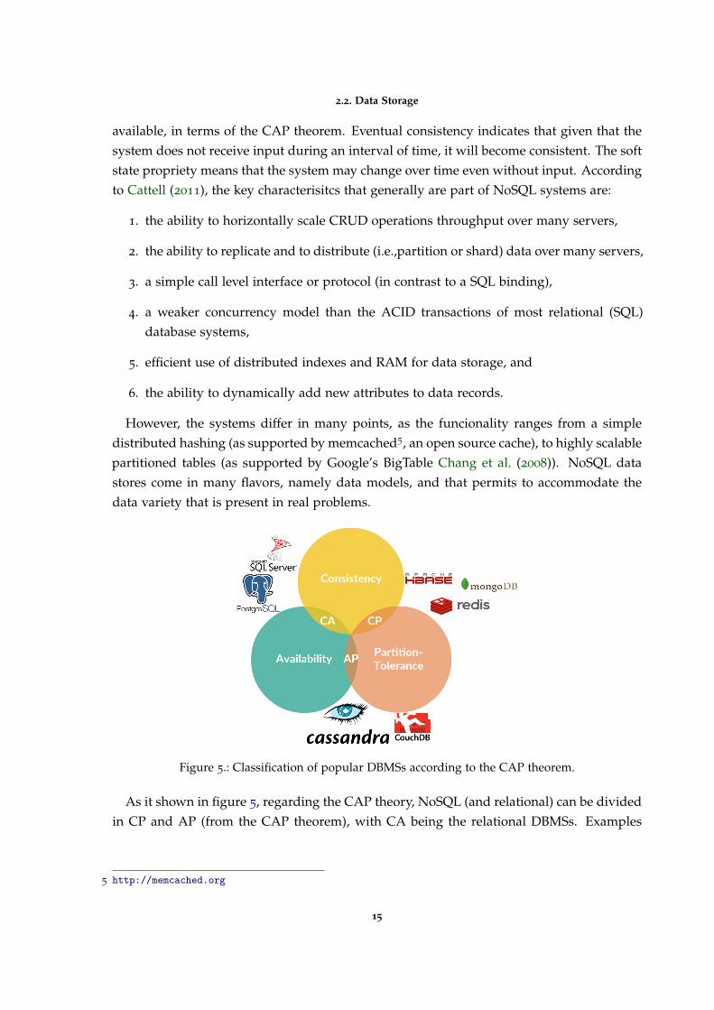
Figure 5.: Classification of popular DBMSs according to the CAP theorem.

As it shown in figure 5, regarding the CAP theory, NoSQL (and relational) can be dividedin CP and AP (from the CAP theorem), with CA being the relational DBMSs. Examples

5 http://memcached.org

15

2.2. Data Storage

of CP systems (that compromise availability) are Apache HBase6, MongoDB7 and Redis8.On the other side, favouring availability and partition-tolerance over consistency (AP) thereis Apache Cassandra9, Apache CouchDB10 and Riak11. Another criterion widely used toclassify NoSQL databases is based on the supported data model. According to this, we candivide the systems in the following categories: Key-value stores, document stores, graphdatabases and wide column stores.

Key-value Stores

The simplest form of database management systems are these. A Key-value DBMS can onlyperform two operations: store pairs of keys and values, and retrieve the stored values givena key. These kind of systems are suitable for applications with simple data models thatrequire a resource-efficient data store like, for example, embedded systems or applicationsthat require a high performance in-process database.

Memcached12 Fitzpatrick (2004) is a high-performance, distributed, memory object cachingsystem, originally designed to speed up web applications by reducing database load. Mem-cached has features similar to other key-value stores: persistence, replication, high availabil-ity, dynamic growth, backups and so on. In Memcached the identification of the destinationserver is done at the client side using a hash function on the key. Therefore, the architectureis inherently scalable as there is no central server to consult while trying to locate valuesfrom keys Jose et al. (2011). Basically, Memcached consists of a client software, which isgiven a list of available memcached servers and a client-based hashing algorithm, whichchooses a server based on the “key” input. On the server side, there is an internal hashtable that stores the values with their keys and an a set of algorithms that determine whento throw out old data or reuse memory.

Another example of a key-value store is Redis (REmote DIctionary Server). Redis is anin-memory database where complex objects such as lists and sets can be associated with akey. In Redis, data may have customizable time-to-live (TTL) values, after which keys areremoved from memory. Redis uses locking for atomic updates and performs asynchronousreplications Khazaei et al. (2015). Redis performs very well compared to writing the datainto the disk for any changes in the data, in applications that do not need durability ofdata. As it is in-memory database, Redis might not be the right option for data-intensive

6 https://hbase.apache.org7 https://www.mongodb.com8 http://redis.io9 http://cassandra.apache.org

10 http://couchdb.apache.org11 http://docs.basho.com/riak/latest/12 http://memcached.org

16

2.2. Data Storage

applications with dominant read operations, because the maximum Redis data set cant bebigger than memory 13.

Document-oriented Databases

Document-oriented databases are, as the name implies, data stores designed to store andmanage documents. Typically, these documents are encoded in standard data exchangeformats such as XML, JSON (Java Script Option Notation), YAML (YAML Ain’t MarkupLanguage), or BSON (Binary JSON). These kind of stores allow nested documents or listsas values as well as scalar values, and the attribute names are dynamically defined for eachdocument at runtime. When comparing to the relational model, we can say that a singlecolumn can hold hundreds of attributes, and the number and type of attributes recordedcan vary from row to row, since its schema free. Unlike key-value stores, these kind ofstores allows to search on both keys and values, and support complex keys and secondaryindexes.

Apache CouchDB14 is a flexible, fault-tolerant database that stores collections, forminga richer data model compared to similar solutions. This solution supports as data formatsJSON and AtomPub15. Queries are done with what CouchDB calls “views”, which are theprimary tool used for querying and reporting, defined with Javascript to specify field con-straints. Views are built on-demand to aggregate, join and report on database documents.The indexes are B-trees, so the results of queries can be ordered or value ranges. Queriescan be distributed in parallel over multiple nodes using a map-reduce mechanism. How-ever, CouchDBs view mechanism puts more burden on programmers than a declarativequery language Foundation (2014).

MongoDB16 is a database that is half way between relational and non-relational systems.Like CouchDB, it provides indexes on collections, it is lockless and it provides a querymechanism. However, there are some differences: CouchDB provides multiversion concur-rency control while MongoDB provides atomic operations on fields; l MongoDB supportsautomatic sharding by distributing the load across many nodes with automatic failoverand load balancing, on the other hand CouchDB achieves scalability through asynchronousreplication Khazaei et al. (2015). MongoDB supports master-slave replication with auto-matic failover and recovery. The data is stored in a binary JSON-like format called BSONthat supports boolean, integer, float, date, string and binary types. The communication ismade over a socket connection (in CouchDB it is made over an HTTP REST interface).

13 http://redis.io/documentation14 http://couchdb.apache.org15 http://bitworking.org/projects/atom/rfc5023.html16 https://www.mongodb.com

17

2.2. Data Storage

Graph-oriented Databases

Graph databases are data stores that employ graph theory concepts. In this model, nodesare entities in the data domain and edges are the relationship between two entities. Nodescan have properties or attributes to describe them. These kind of systems are used forimplementing graph data modeling requirements without the extra layer of abstraction forgraph nodes and edges. This means less overhead for graph-related processing and moreflexibility and performance.

Neo4j17 is the most known and used graph storage project. It has various native APIs inmost of programming languages such as Java, Go, PHP, and others. Neo4j is fully ACIDcompatible and schema-free. Additionally, it uses its own query language called Cypherthat is inspired by SQL, and supports syntax related to graph nodes and edges. Neo4j doesnot allow data partiitioning, and this means that data size should be less than the capacityof the server. However, it supports data replication in a master-slave fashion which ensuresfault tolerance against server failures.

Column-oriented Databases

Column-oriented databases are the kind of data store that most resembles the relationalmodel on a conceptual level. They retain notions of tables, rows and columns, creatingthe notion of a schema, explicit from the client’s perspective. However, the design princi-ples, architecture and implementation are quite different from traditional RDBMS. Whilethe notion of tables’ main function is to interact with clients, the storage, indexing and dis-tribution of data is taken care by a file and a management system. In this approach, rowsare split across nodes through sharding on the primary key. They typically split by rangerather than a hash function. This means that queries on ranges of values do not have to goto every node. Columns of a table are distributed over multiple nodes by using “columngroups”. These may seem like a new complexity, but column groups are simply a way forthe customer to indicate which columns are best stored together Cattell (2011). Rows areanalogous to documents: they can have a variable number of attributes (fields), the attributenames must be unique, rows are grouped into collections (tables), and an individual row’sattributes can be of any type. For applications that scan a few columns of many rows, theyare more efficient, because this kind of operations lead to less loaded data than reading thewhole row. Most wide-column data store systems are based on a distributed file system.Google BigTable, the precursor of the popular data store systems of this kind, is built ontop of GFS (Google File System).

Apache HBase is the NoSQL wide-column store for Hadoop, the open-source implemen-tation of MapReduce for Big Data analytics. The purpose of HBase is to support random,

17 http://neo4j.com

18

2.2. Data Storage

real-time read and write access to very large tables with billions of rows and millions ofcolumns. HBase uses the Hadoop distributed file system in place of the Google file system.It puts updates into memory and periodically writes them out to files on the disk. Rowoperations are atomic, with row-level locking and transactions. Partitioning and distribu-tion are transparent; there is no client-side hashing or fixed keyspace as in some NoSQLsystems. There is multiple master support, to avoid a single point of failure. MapReducesupport allows operations to be distributed efficiently.

Apache Cassandra is designed under the premise that failures may happen both in soft-ware and hardware, being practically inevitable. It has column groups, updates are cachedin memory and then flushed to disk, and the disk representation is periodically compacted.It does partitioning and replication. Failure detection and recovery are fully automatic.However, Cassandra has a weaker concurrency model than some other systems: there is nolocking mechanism, and replicas are updated asynchronously.

Comparative Evaluation of NoSQL Databases

As it was presented, there are several options when it comes the time to choose a NoSQLdatabase, and the different categories and architectures serve different purposes. Althoughfour categories were presented, only two of them are adequate for the purposes of thiswork. Regarding support for complex queries column-oriented and document-orienteddata store systems are more adequate than key-value stores (e.g. simple hash tables) andgraph databases (which are ideal for situations that are modeled as graph problems). Con-sidering the last presented fact, we selected Apache Cassandra, CouchDB, Apache HBaseand MongoDB as the object of this evaluation. The following table is based in the workpresented in Lourenco et al. (2015), where several DBMS are classified in a 5-point scale(Great, good, average, mediocre and bad) regarding a set of quality atributes.

DBMS Cassandra CouchDB HBase MongoDBAvailability Great Great Mediocre MediocreConsistency Great Good Average GreatDurability Mediocre Mediocre Good Good

Maintainability Good Good Mediocre AverageRead-Performance Good Average Mediocre Great

Recovery Time Great Unknown Unknown GreatReliability Mediocre Good Good GreatRobustness Good Average Bad AverageScalability Great Mediocre Great Mediocre

Stabilization Time Bad Unknown Unknown BadWrite-Performance Good Mediocre Good Mediocre

Table 1.: NoSQL DBMS comparison.

19

2.3. Data Analytics

As it is mentioned in Lourenco et al. (2015), the follwing criteria were used:

AVAILABILITY the downtime was used as a primary measure, together with relevant studiessuch as Nelubin and Engber (2013).

CONSISTENCY was graded according to how much the database can provide ACID-semanticsand how much can consistency be fine-tuned.

DURABILITY was measured according to the use of single or multi version concurrencycontrol schemes, the way that data are persisted to disk (e.g. if data is always asyn-chronously persisted, this hinders durability), and studies that specifically targeteddurability.

MAINTAINABILITY the currently available literature studies of real world experiments, theease of setup and use, as well as the accessibility of tools to interact with the database.

READ AND WRITE PERFORMANCE the grading of this point was done by considering recentstudies (Nelubin and Engber (2013)) and the fine-tuning of each database.

RELIABILITY is graded by looking at synchronous propagation modes.

ROBUSTNESS was assessed with the real world experiments carried by researchers, as wellas the available documentation on possible tendency of databases to have problemsdealing with crashes or attacks.

SCALABILITY was assessed by looking at each database’s elasticity, its increase in perfor-mance due to horizontal scaling, and the ease of live addition of nodes.

STABILIZATION AND RECOVERY TIME this measure is highly related to availability and is basedour classification on the results shown in Nelubin and Engber (2013).

Although there have been a variety of studies and evaluations of NoSQL technology,there is still not enough information to verify how suited each non-relational database is ina specific scenario or system. Moreover, each working system differs from another and allthe necessary functionality and mechanisms highly affect the database choice. Sometimesthere is no possibility of clearly stating the best database solution Lourenco et al. (2015).

2.3 data analytics

Data analytics encomprises the set of complex procedures running over large-scale, datarepositories (like big data repositories) whose main goal is that of extracting useful knowl-edge kept in such repositories Cuzzocrea et al. (2011). Along with the storage problem(conveying big data stored in heterogeneous and different-in-nature data sources into a

20

2.3. Data Analytics

structured format), the issue of processing and transforming the extracted structured datarepositories in order to derive Business Intelligence (BI) components like diagrams, plots,dashboards, and so forth, for decision making purposes, is the most addressed aspect byorganizations.

In this section, one of the most widely used tool for data aggregation, Hadoop MapRe-duce Framework18 (and its programming modet that enables parallel and distributed dataprocessing) is introduced, alongside with its architecture. MongoDB Aggregation Frame-work is also introduced as it provides a recent and different approach by providing a toolfor data aggregation contained in the database environment. Additionally, the concept ofReal-time analytics is explored and examples of supporting tools are provided.

2.3.1 MapReduce

MapReduce is a scalable and fault-tolerant data processing tool that enable the processingof massive volumes of data in parallel with many low-end computing nodes Lee et al.(2012). In the context of Big Data analytics, MapReduce presents an interesting modelwhere data locality is explored to improve the performance of applications. The main ideaof the MapReduce model is to hide details of parallel execution, allowing the users to focuson data processing strategies. MapReduce utilizes the GFS while Hadoop MapReduce, thepopular open source alternative, runs above the HDFS.

The computation takes a set of input key/value pairs, and produces a set of outputkey/value pairs. The MapReduce model consists of two primitive functions: Map andReduce. Map, written by the user, takes an input pair and produces a set of intermediatekey/value pairs. The MapReduce library groups together all intermediate values associatedwith the same intermediate key and passes them to the Reduce function. The Reduce functionaccepts an intermediate key and a set of values for that key. It merges together these valuesto form a possibly smaller set of values. Typically just zero or one output value is producedper Reduce invocation. The intermediate values are supplied to the user’s reduce functionvia an iterator. This allows the handling of lists of values that are too large to fit in memoryDean and Ghemawat (2008). The following example (see figure 7) is about the problem ofcounting the number of occurrences of each word in a large collection of documents.

18 https://hadoop.apache.org/docs/current/hadoop-mapreduce-client/hadoop-mapreduce-client-core/MapReduceTutorial.html

21

2.3. Data Analytics

Figure 6.: Hadoop MapReduce architecture.

map(String key , String value):

// key: document name

// value: document contents

for each word w in value:

EmitIntermediate(w, "1");

reduce(String key , Iterator values):

// key: a word

// values: a list of counts

int result = 0;

for each v in values:

result += ParseInt(v);

Emit(AsString(result));

Figure 7.: Pseudocode representing a words counting implementation in map-reduce.

The main advantages of using MapReduce are its simplicity and ease of use, being storageindependent (can work with different storage layers), its fault tolerance and providing high-scalability. On the other hand, there are some pitalls, such as: the lack of a high-levellanguage, being schema-free and index-free, lack of maturity and the fact that operationsnot being always optimized for I/O efficiency. Lee et al. (2012).

22

2.3. Data Analytics

2.3.2 Real Time Analytics

In the spectrum of analytics two extremes can be identified. On one end of the spectrumthere is batch analytical applications, which are used for complex, long-running analyses.Generally, these have slower response times (hours or days) and lower requirements foravailability. Hadoop-based workloads are an example of batch analytical applications. Onthe other end of the spectrum sit real-time analytical applications. Real-time can be consid-ered from the point of view of the data or from the point of view of the end-user. The earliertranslates into the ability of processing data as it arrives, making it possible to aggregatedata and extract trends about the actual situation of the system (streaming analytics). Theformer refers to the ability to process data with low latency (processing huge amount ofdata with the results being available for the end user almost in real-time) making it possible,for example, to to provide recommendations for an user on a website based on its historyor to do unpredictable, ad hoc queries against large data sets (online analytics).

Regarding stream processing the main problems are related to: Sampling Filtering, Cor-relation, Estimating Cardinality, Estimating Quantiles, Estimating Moments, Finding Fre-quent Elements, Counting Inversions, Finding Subsequences, Path Analysis, Anomaly De-tection Temporal Pattern Analysis, Data Prediction, Clustering, Graph analysis, Basic Count-ing and Significant Counting. The main applications are A/B testing, set membership,fraud detection, network analysis, traffic analysis, web graph analysis, sensor networksand medical imaging (Kejariwal et al. (2015)).

According to Kejariwal et al. (2015) these are the most well-known streaming open sourcetools:

S4 Real-time analytics with a key-value based programming model and support for schedul-ing/message passing and fault tolerance.

STORM The most popular and widely adopted real-time analytics platform developed atTwitter.

MILLWHEEL Google’s proprietary realtime analytics framework thats provides exact oncesemantics.

SAMZA Framework for topology-less real-time analytics that emphasizes sharing betweengroups.

AKKA Toolkit for writing distributed, concurrent and fault tolerant applications.

SPARK Does both offline and online analysis using the same code and same system.

FLINK Fuses offline and online analysis using traditional RDBMS techniques.

PULSAR Does real-time analytics using SQL.

23

2.3. Data Analytics

HERON Storm re-imagined with emphasis on higher scalability and better debuggability.

Online analytics, on the other hand, are designed to provide lighter-weight analytics veryquickly. The requirements of this kind of analytics are low latency and high availability. Inthe Big Data era, OLAP (on-line analytical processing Chaudhuri and Dayal (1997)) andtraditional ETL processes are too expensive. Particularly, the heterogeniety of the datasources difficults the definition of rigid schemas, making model-driven insight difficult.In this paradigm analytics are needed in near real time in order to support operationalapplications and their users. This includes applications from social networking news feedsto analytics, from real-time ad servers to complex CRM applications.

2.3.3 MongoDB Aggregation Framework

MongoDB is actually more than a data storage engine, as it also provides native data pro-cessing tools: MapReduce19 and the Aggregation pipeline20. Both the aggregation pipelineand map-reduce can operate on a sharded collection (partitioned over many machines, hor-izontal scaling). These are powerful tools for performing analytics and statistical analysisin real-time, which is useful for ad-hoc querying, pre-aggregated reports, and more. Mon-goDB provides a rich set of aggregation operations that process data records and returncomputed results, using this operations in the data layer simplifies application code andlimits resource requirements. The documentation of MongoDB provides a comparison ofthe different options of aggregation commands21.

The Aggregation pipeline (introduced in MongoDB 2.2) is based on the concept of dataprocessing pipelines (analogous to the unix pipeline). The documents are processed in amulti-stage pipeline that produces the aggregated results. Each stage transforms the doc-uments as they pass through the pipeline. Output of first operator will be fed as input tothe second operator and so on. Despite, being limited to the operators and expressions sup-ported, the aggregation pipeline can add computed fields, create new virtual sub-objects,and extract sub-fields into the top-level of results by using the project22 pipeline operator.

Follwing the pipeline architecture pattern, expressions can only operate on the currentdocument in the pipeline and cannot refer to data from other documents: expression op-erations provide in-memory transformation of documents. Expressions are stateless andare only evaluated when seen by the aggregation process with one exception: accumulatorexpressions. The accumulators, used in the group23 stage of the pipeline, maintain theirstate (e.g. totals, maximums, minimums, and related data) as documents progress through

19 https://docs.mongodb.org/manual/core/map-reduce/20 https://docs.mongodb.org/manual/core/aggregation-pipeline/21 https://docs.mongodb.org/manual/reference/aggregation-commands-comparison/22 https://docs.mongodb.org/manual/reference/operator/aggregation/project/#pipe._S_project23 https://docs.mongodb.org/manual/reference/operator/aggregation/group/#pipe._S_group

24

2.4. Machine Learning

Figure 8.: MongoDB Aggregation Pipeline example.

the pipeline. In version 3.2 (the most recent) some accumulators are available in the projectstage, but it this situation they do not maintain their state across documents.

2.4 machine learning

In this section, an introduction to the current state of machine learning will be provided.This review will follow a top-down approach. The basic concepts of learning will be intro-duced, and further in the section an overview of deep neural networks (the main theoreticaltopic driving machine learning research) will be presented, essentialy from a user perspec-tive. The goal here is to provide insight on how the current machine learning techniquesare located in the big data scene, what to expect from them in the near future and howcould they help to provide real-time intelligence.

2.4.1 Introduction to Learning

A computer program is said to learn from experience E with respect to some class of tasksT and performance measure P if its performance at tasks in T, as measured by P, improveswith experience E (Mitchell (1997)). From this formal definition of machine learning, ageneralization can be made categorizing such systems as systems that automatically learn

25

2.4. Machine Learning

programs from data (Domingos (2012)). As the data volumes grow rapidly this premisebecomes more and more attractive, providing alternative to manually constructing the de-sired programs. Among other domains Machine learning is used in Web search, spamfilters, recommender systems, ad placement, credit scoring, fraud detection, stock trading,drug design, among others.

Generally, learning algorithms consist of combinations of just three components. For eachof the components the list of options is very large resulting in a variety of machine learningalgorithms that is in the order of magnitude of the thousands. The three components aredescribed below (Domingos (2012)):

REPRESENTATION A classifier must be represented in some formal language that the com-puter can handle. Conversely, choosing a representation for a learner is equivalent tochoosing the set of classifiers that it can possibly learn. This set is called the hypoth-esis space of the learner. The crucial question at this stage is how to represent theinput, i.e., what features to use.

EVALUATION An evaluation function (also called objective function or scoring function) isneeded to distinguish good classifiers from bad ones. Examples of evaluation func-tions are: accuracy/error rate, precision and recall, squared error, and likelihood.

OPTIMIZATION a method to search among the classifiers in the language for the highest-scoring one. The choice of optimization technique is key to the efficiency of thelearner, and also helps determine the classifier produced if the evaluation functionhas more than one optimum. The optimization methods are can be combinatorial(greedy search, beam search, branch-and-bound) or continuous (gradient descent,quasi-newton methods, linear and quadratic programming).

Many different types of machine learning exist, such as clustering, classification, regres-sion and density estimation. There is a fundamental difference on the types of algorithmsthat is related to goals of the learning process. In order to illustrate these differences, thedefinitions of clustering (unsupervised learning) and classification (supervised learning)are hereby presented (Bagirov et al. (2003)).

Clustering names the process of identification of subsets of the data that are similarbetween each other. Intuitively, a subset usually corresponds to points that are more similarto each other than they are to points from another cluster. Points in the same cluster aregiven the same label. Clustering is carried out in an unsupervised way by trying to findsubsets of points that are similar without having a predefined notion of the labels.

26

2.4. Machine Learning

Classification, on the other hand, involves the supervised assignment of data points topredefined and known classes. It is the most mature and widely used type of machinelearning. In this case, there is a collection of classes with labels and the goal is to labela new observation or data point as belonging to one or more of the classes. The knownclasses of examples constitute a training set and are used to learn a description of the classes(determined by some a priori knowledge about the dataset). The trained artifact can thenbe used to assign new examples to classes.

Another definition that is relevant in this context is the concept of reinforcement learn-ing, that is much more focused on goal-directed learning from interaction than are otherapproaches to machine learning. Reinforcement learning is a formal mathematical frame-work in which an agent manipulates its environment through a series of actions, and inresponse to each action, receives a reward value. An agent stores its knowledge about howto choose reward-maximizing actions in a mapping form agent-internal states to actions.In essence, the agent’s “task” is to maximize reward over time. Good task performance isprecisely and mathematically defined by the reward values (McCallum (1996)).

The goal of these kind of algorithms is to obtain a generalization, however no matterhow much data is available, data alone is not enough. Every learner must embody someknowledge or assumptions beyond the data it’s given in order to generalize beyond it. Thiswas formalized by Wolpert in his famous “no free lunch” theorems, according to which nolearner can beat random guessing over all possible functions to be learned (Wolpert (1996)).

The catch here is the fact that the functions to be learned in the real world are notdrawn uniformly from the set of all mathematically possible functions. In fact, very generalassumptions are often enough to do very well, and this is a large part of why machinelearning has been so successful.

The main problems associated with learning algorithms are the possibility of overfittingover the training data and the “curse” of dimensionality Bellman (1961).

Overfitting it comes in many forms that are not immediately obvious. When a learneroutputs a classifier that fits all the training data but fails on most of the data from the testdataset, it has overfit. One way to understand overfitting is by decomposing generalizationerror into bias and variance (see figure 9). Bias is a learner’s tendency to consistently learnthe same wrong thing. Variance is the tendency to learn random things irrespective ofthe real signal. It’s easy to avoid overfitting (variance) by falling into the opposite error ofunderfitting (bias). Simultaneously avoiding both requires learning a perfect classifier, andshort of knowing it in advance there is no single technique that will always do best (no freelunch). Generalizing correctly becomes exponentially harder as the dimensionality (numberof features) of the examples grows, because a fixed-size training set covers a very smallfraction of the input space. Fortunately, there is an effect that partly counteracts the curseas in most applications examples are not spread uniformly throughout the instance space,

27

2.4. Machine Learning

but are concentrated on or near a lower-dimensional manifold. Learners can implicitlytake advantage of this lower effective dimension, or algorithms for explicitly reducing thedimensionality can be used.

Figure 9.: Bias and variance in dart-throwing (Domingos (2012)).

In the Big Data context, data mining techniques and machine learning algorithms havebeen very useful in order to make use of complex data, bringing exciting opportunities. Forexample, researchers have successfully used Twitter to detect events such as earthquakesand major social activities, with nearly online speed and very high accuracy. In addition,the knowledge of people’s queries to search engines also enables a new early warningsystem for detecting fast spreading flu outbreaks (Wu et al. (2014)).

2.4.2 Deep Neural Network Architecutres

The recent vast research activities in neural classification have established that neural net-works are a promising alternative to various conventional classification methods. The ad-vantage of neural networks lies in four theoretical aspects.

• Neural networks are data driven self-adaptive methods in that they can adjust them-selves to the data without any explicit specification of functional or distributionalform for the underlying model.

• They are universal functional approximators, meaning that neural networks can ap-proximate any function with arbitrary accuracy.

28

2.4. Machine Learning

• Neural networks are nonlinear models, which makes them flexible in modeling realworld complex relationships.

• Neural networks are able to estimate the posterior probabilities, which provides thebasis for establishing classification rule and performing statistical analysis.

A standard neural network (NN) consists of many simple, connected processors calledneurons, each producing a sequence of real-valued activations. Input neurons get acti-vated through sensors perceiving the environment (x, y and z), other neurons get activatedthrough weighted connections (a values) from previously active neurons (as it is shown onfigure 10).

Figure 10.: Functional model of an artificial neural network (Rojas (2013)).

Learning or credit assignment is about finding weights (a values) that make the networkexhibit desired behavior. Depending on the problem and how the neurons are connected,such behavior may require long causal chains of computational stages, where each stagetransforms the aggregate activation of the network (Schmidhuber (2015)). Therefore, in anymodel of artficial neural networks there are three elements that are particularly important(Rojas (2013)): the structure of the nodes, the topology of the network and the learningalgorithm used to find the weights of the network.

In recent years, deep artificial neural networks (including recurrent ones) have wonnumerous contests in pattern recognition and machine learning. Training of deep neuralnetworks with many layers had been found to be difficult in practice by the late 1980s(Sec. 5.6), and had become an explicit research subject by the early 1990s. However since2000s, deep learning have finally attracted wide-spread attention, mainly by outperformingalternative machine learning methods such as kernel machines in numerous importantapplications. In fact, since 2009, supervised deep NNs have won many official internationalpattern recognition competitions, achieving the first superhuman visual pattern recognitionresults in limited domains (Rojas (2013)).

These type of architectures are more efficient for representing certain classes of functions,particularly those involved in visual recognition. A deep architecture trades space for time

29

2.4. Machine Learning

(or breadth for depth), more layers (more sequential computation), but less hardware (lessparallel computation), LeCun et al. (2015).

2.4.3 Popular Frameworks and Libraries

Given the current success of deep learning techniques on machine learning tasks, its usehas become more widespread. In this subsection the goal is to show some examples ofpopular frameworks and libraries that support deep learning, particularly deep neural net-works. The list of available frameworks includes, but is not limited to, Caffe, DeepLearn-ing4J, deepmat, Eblearn, Neon, PyLearn, TensorFlow, Theano, Torch. Different frameworkstry to optimize different aspects of training or deployment of a deep learning algorithm(Bahrampour et al. (2015)).

TensorFlow is an interface for expressing machine learn- ing algorithms, and an imple-mentation for executing such algorithms. A computation expressed using TensorFlow canbe executed with little or no change on a wide variety of hetero- geneous systems, rangingfrom mobile devices such as phones and tablets up to large-scale distributed systems of hun-dreds of machines and thousands of computational devices such as GPU cards. The systemis flexible and can be used to express a wide variety of algorithms, including training andinference algorithms for deep neural network models, and it has been used for conductingresearch and for deploying machine learning systems into production across more than adozen areas of computer science and other fields, including speech recognition, computervision, robotics, information retrieval, natural language processing, geographic informationextraction, and computational drug discovery (Abadi et al. (2016)).

Theano is a framework in the Python programming language for defining, optimizingand evaluating expressions involving high-level operations on tensors. Theano offers mostof NumPy’s functionality, but adds automatic symbolic differentiation, GPU support, andfaster expression evaluation. Theano is a general mathematical tool, but it was developedwith the goal of facilitating research in deep learning (Bergstra et al. (2011)).

DeepSpark is a distributed and parallel deep learning framework that simultaneously ex-ploits Apache Spark for large-scale distributed data management and Caffe for GPU-basedacceleration. DeepSpark directly accepts Caffe input specifications, providing seamlesscompatibility with existing designs and network structures (Kim et al. (2016)).

H2O24 is a open source math engine for big data that computes parallel distributedmachine learning algorithms. It is distributed as an R package. H2O supports a number ofstandard statistical models, such as GLM, K-means, and Random Forest. H2O is nurturinga grassroots movement of physicists, mathematicians, and computer scientists to herald the

24 http://www.h2o.ai

30

2.5. Related Projects

new wave of discovery with data science by collaborating closely with academic researchersand Industrial data scientists Arora et al. (2015).

2.5 related projects

In this section will be presented current projects from different domains that share some ofthe technical challenges with the defined goal project of this dissertation.

2.5.1 Financial Services - MetLife25

MetLife is an insurance company that has more than 100 million clients as individuals. Itsnew subsystem called “The Wall” was in production across MetLife’s call centers. The Wallcollects vast amounts of structured and unstructured information from MetLife’s more than70 different administrative systems. When a customer calls MetLife to ask about a claim,add a new baby to a policy, or dig into coverage details, the customer representatives use theWall to pull up every bit of information they need in seconds – name, address, policies, andlife events. The challenges here are related to data variety and velocity (on ad-ho queries).Right now, MetLife is creating a real-time analytical system that predicts customer attritionrates, prompting customer reps to offer alternative products or promotions. AdditionallyMetLife is considering adding social data and data from mobile apps into The Wall to gainan even better understanding of customers.

2.5.2 Government - The City of Chicago

Event capture and analysis, crime data management and analytics, citizen engagementplatforms, entity catalog and healthcare record management are some of the use cases forGoverment that require Big Data capabilities. An example of a stakeholder for such usecases is The City of Chicago26. WindyGrid (from the city of Chicago) is a system that itpulls together seven million different pieces of data from city departments every day, andpowers the users with analytics (with visual maps), giving managers insights in real timeon city operations. Roadwork updates, trash pickup delays, 911 health emergencies, 311

complaints about noise, public tweets about the minutia of the city’s workings, bus locationsalong their route, traffic light patterns, are collected and are integrated into a real-timegeospatial platform. This platform enables the identification of unexpected correlations andpotential issues before they develop into bigger problems, and helps coordinate responsesamong departments to everything from marathons to major snowstorms.

25 http://global.metlife.com26 https://www.mongodb.com/customers/city-of-chicago

31

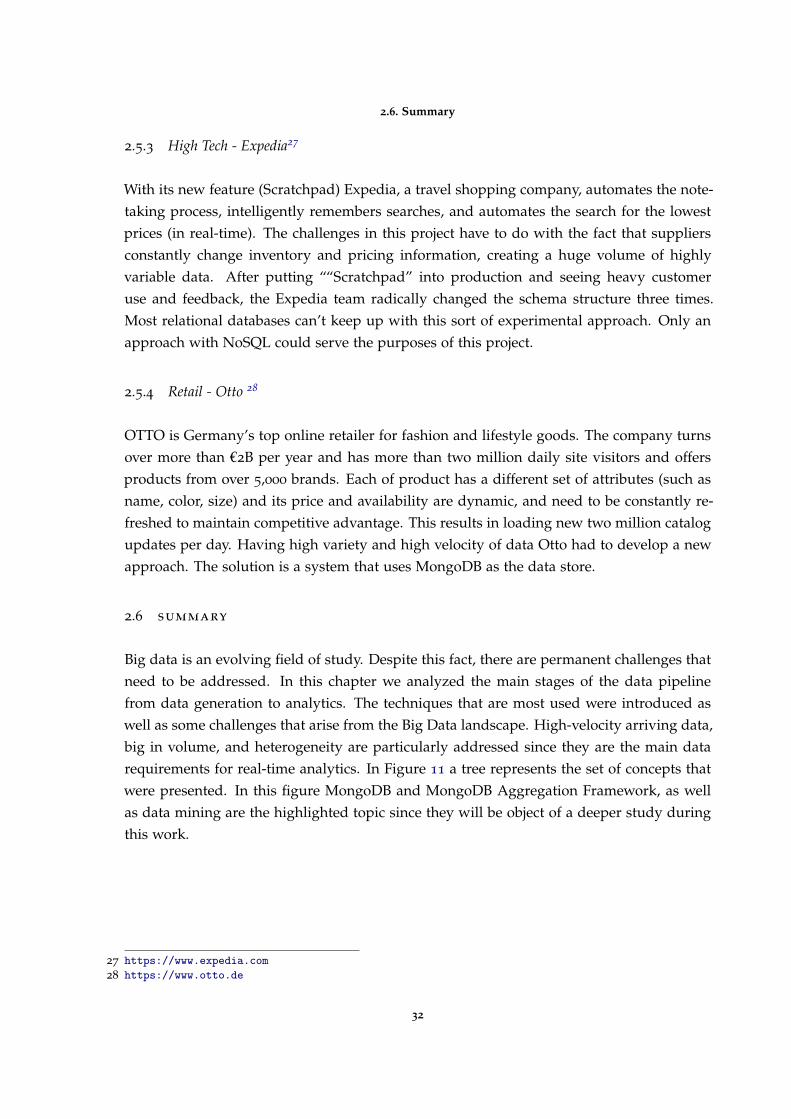
2.6. Summary

2.5.3 High Tech - Expedia27

With its new feature (Scratchpad) Expedia, a travel shopping company, automates the note-taking process, intelligently remembers searches, and automates the search for the lowestprices (in real-time). The challenges in this project have to do with the fact that suppliersconstantly change inventory and pricing information, creating a huge volume of highlyvariable data. After putting ““Scratchpad” into production and seeing heavy customeruse and feedback, the Expedia team radically changed the schema structure three times.Most relational databases can’t keep up with this sort of experimental approach. Only anapproach with NoSQL could serve the purposes of this project.

2.5.4 Retail - Otto 28

OTTO is Germany’s top online retailer for fashion and lifestyle goods. The company turnsover more than †2B per year and has more than two million daily site visitors and offersproducts from over 5,000 brands. Each of product has a different set of attributes (such asname, color, size) and its price and availability are dynamic, and need to be constantly re-freshed to maintain competitive advantage. This results in loading new two million catalogupdates per day. Having high variety and high velocity of data Otto had to develop a newapproach. The solution is a system that uses MongoDB as the data store.

2.6 summary

Big data is an evolving field of study. Despite this fact, there are permanent challenges thatneed to be addressed. In this chapter we analyzed the main stages of the data pipelinefrom data generation to analytics. The techniques that are most used were introduced aswell as some challenges that arise from the Big Data landscape. High-velocity arriving data,big in volume, and heterogeneity are particularly addressed since they are the main datarequirements for real-time analytics. In Figure 11 a tree represents the set of concepts thatwere presented. In this figure MongoDB and MongoDB Aggregation Framework, as wellas data mining are the highlighted topic since they will be object of a deeper study duringthis work.

27 https://www.expedia.com28 https://www.otto.de

32

2.6. Summary

Figure 11.: Overview of the concepts presented in chapter 2.

33

3

T H E P R O B L E M A N D I T S C H A L L E N G E S

With the advent of the Internet of Things the number of devices that are connected isincreasing every day. Consequently, the number of interactions that can generate data isgrowing as well. Humans tend to show their personality or their state through their actions,even in an unconscious way. Facial expressions and body language, for example, have beenknown as a gateway for feelings that result in intentions. The resultant actions can be tracedto a certain behavior. Therefore, it is safe to assume that a human behavior can be outlinedeven if the person does not want to explicitly share that information.

The interaction with computers and other technological devices can provide dataset con-taining records that are relative to unconscious behaviors. The rhythm at which a persontypes on a keyboard or the movement of the mouse changes when the individual becomesfatigued or under severe stress, as it was established in Pimenta et al. (2013); Carneiro et al.(2012). Moreover, the interaction with smartphones can also provide analogous patternsfrom diverse sources including a touchscreen (that provides information about touches,their intensities, their area or their duration), gyroscopes, accelerometers, among others.

Gathering metrics on people’s behaviours and providing tools for visualization, particu-larly real time analytics, enables decision making and data-driven actions concerning well-being of individuals (Carneiro et al. (2016)). The trend for data collection regarding sensingon humans is growing and the perspective is for this trend to keep strong, giving the ex-pected growth of IoT (Internet of Things). Furthermore, Big Data tools and techniquesenable for this to be done at a large scale without compromising performance and availabil-ity.

According to Pimenta et al. (2013), by recording the data from the keyboard and mousemovements it is possible to metrics that enable the prediction of fatigue levels. In thispaper the authors introduce a monitoring system for mental fatigue. The system works ina non-invasive way, by analysing a set of features that are acquired from the individual’sregular use of a computer (namely from the mouse and the computer). The mental fatigueis quantified by a classifier. By going through a prior learning phase on historical data, thesystem learns on how to classify the fatigue of an individual user.

Particularly, the following features are considered Pimenta et al. (2013):

34

KEYDOWN TIME time spent between the key down and the key up events;

ERRORS PER KEY PRESSED number of times the backspace key is pressed, versus the keyspressed;

MOUSE VELOCITY velocity at which the cursor travels;

MOUSE ACCELERATION acceleration of the mouse at a given time;

TIME BETWEEN KEYS time spent between each two keys pressed;

TOTAL EXCESS OF DISTANCE excess of distance travelled by the pointer when considering twoconsecutive clicks;

AVERAGE EXCESS OF DISTANCE average of the distance excess travelled by the pointer whenconsidering two consecutive clicks;

DOUBLE CLICK SPEED speed of the double click;

NUMBER OF DOUBLE CLICKS number of double clicks in a time frame;

DISTANCE WHILE CLICKING distance travelled by the mouse while dragging objects;

SIGNED SUM OF ANGLES how much the pointer “turned” left or right during its travel;

ABSOLUTE SUM OF ANGLES how much the pointer “turned” during its travel, in absoluteterms;

SUM OF DISTANCES BETWEEN PATH AND STRAIGHT LINE considering two consecutive clicks, it mea-sures the distance between all the points of the path travelled by the mouse, and theclosest point in a straight line (that represents the shortest path) between the coordi-nates of the two clicks;

AVERAGE DISTANCE BETWEEN PATH AND STRAIGHT LINE the same as above, but provides an av-erage value of the distance to the straight line;

TIME BETWEEN CLICKS time spent between each two clicks.

By evaluating the mental performance, a sense of the plain use of cognitive skills byan individual can be acquired, and with this information optimize the productivity of anindividual while carrying sensitive tasks. This approach also takes a step forward on thedevelopment of intelligent working environments, that can take actions on the insightsobtained from workers’ behaviours and improve the quality of life and their performanceon tasks in which they are engaged.

The potential of applying this system in large scale is enormous and Performetric (indevelopment since the August of 2015) is a company that works in order to do so. The

35

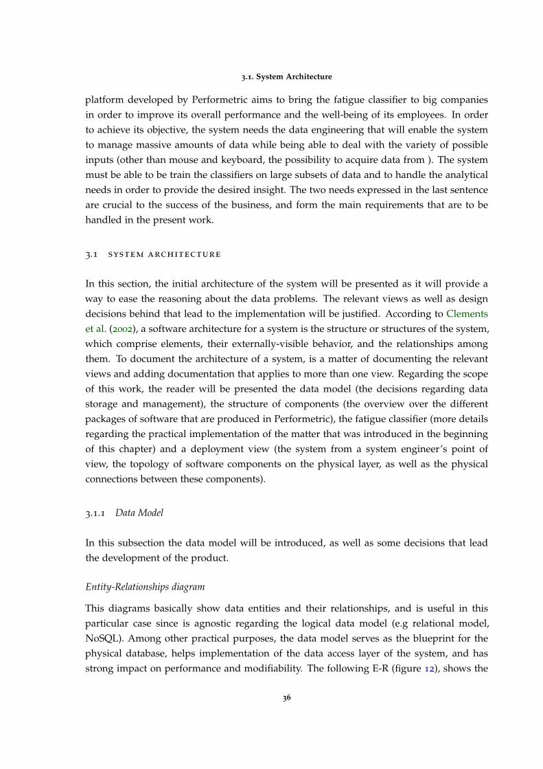
3.1. System Architecture

platform developed by Performetric aims to bring the fatigue classifier to big companiesin order to improve its overall performance and the well-being of its employees. In orderto achieve its objective, the system needs the data engineering that will enable the systemto manage massive amounts of data while being able to deal with the variety of possibleinputs (other than mouse and keyboard, the possibility to acquire data from ). The systemmust be able to be train the classifiers on large subsets of data and to handle the analyticalneeds in order to provide the desired insight. The two needs expressed in the last sentenceare crucial to the success of the business, and form the main requirements that are to behandled in the present work.

3.1 system architecture

In this section, the initial architecture of the system will be presented as it will provide away to ease the reasoning about the data problems. The relevant views as well as designdecisions behind that lead to the implementation will be justified. According to Clementset al. (2002), a software architecture for a system is the structure or structures of the system,which comprise elements, their externally-visible behavior, and the relationships amongthem. To document the architecture of a system, is a matter of documenting the relevantviews and adding documentation that applies to more than one view. Regarding the scopeof this work, the reader will be presented the data model (the decisions regarding datastorage and management), the structure of components (the overview over the differentpackages of software that are produced in Performetric), the fatigue classifier (more detailsregarding the practical implementation of the matter that was introduced in the beginningof this chapter) and a deployment view (the system from a system engineer’s point ofview, the topology of software components on the physical layer, as well as the physicalconnections between these components).

3.1.1 Data Model

In this subsection the data model will be introduced, as well as some decisions that leadthe development of the product.

Entity-Relationships diagram

This diagrams basically show data entities and their relationships, and is useful in thisparticular case since is agnostic regarding the logical data model (e.g relational model,NoSQL). Among other practical purposes, the data model serves as the blueprint for thephysical database, helps implementation of the data access layer of the system, and hasstrong impact on performance and modifiability. The following E-R (figure 12), shows the

36

3.1. System Architecture

main entities in the system from the data engineer point of view, some entities referringto the operationality of the apps were excluded (session and login data, for example) forclarity purposes.

Figure 12.: Conceptual Diagram of the Data Model (according to Chen (1976)).

The diagram is self explanatory regarding the relationships between entities, howeversome details must be clarified regarding the entities themselves. As it is shown in figure12, the User is the central entity of the diagram. This entity contains all the attributes thatdescribe the user (personal info such age, sex and attributes regarding the machine). A useris associated with a company (and with a team within a company) and contains data relatedto the fatigue alerts (issued when a user fatigue level goes beyond the defined threshold)and break times (recorded when a user takes a break in the 30 minutes after a fatiguealert). The MouseDynamics and KeyboardDynamics entities represent the data generatedby the user interaction with the mouse and keyboard, respectively. The data in the previousentities is pre-processed and then is applied to the classifier, generating a BiometricRecordthat contains the fatigue level average calculated in 5 minutes intervals.

Storage Decisions

The decision regarding the database management system present in this system is major asthe database will be under intense write operations loads and is also the basis for analyticalpurposes. As it was presented in the literature review chapter, conventional databases arelimited regarding flexibility (capacity to deal with semi-structured or unstructured data)issues. Also, the relational model shortcomings on scalability frequently cause bottleneckson big data projects. Having this in mind, and the requirement of a document-orienteddatabase imposed by the development team, there was a last factor that determined the

37

3.1. System Architecture

decision. According to the comparison presented on Chapter 2, MongoDB is the best optionregarding read-performance, reliability, consistency and durability, and these criteria wereconsidered as they relate to the analytical capabilities of a database management system.

3.1.2 System Components

The following diagram has the goal of showing the different modules that constitute the Per-formetric software. The software product follows the layered architecture pattern. Withineach layer, functionality is related by a common role or responsibility. Communicationbetween layers is explicit and loosely coupled. The diagram in figure 13 represents strictlayering (Bass et al. (2012)), meaning that components in one layer can interact only withcomponents direct below it. Inside each layer the software is divided in modules accordingto its functionality. The division in modules is made according to the loose coupling, highcohesion principle Bass et al. (2012).

Figure 13.: The deplyment view (showing the layered architecture).

The first implemented layer was the data generation layer. The raw data is generated inthe devices, then pre-processed (applying redundancy elimination techniques such as dataaggregation and measurements) and stored locally whenever possible (as in smartphonesand personal computers) in a SQLite database. The names of the modules in this layer

38

3.1. System Architecture

are self-explanatory, and relate directly to the implemented software packages (currentlyimplemented in Objective-C on OSX, and C# on Windows).

The classification layer contains all the software related to the mental fatigue prediction.This layer contains three modules, being the training and the classifier module the imple-mentation of the learning system and the communication module related to the networkAPI with which the other modules communicate. The classifier is implemented in the Rlanguage1.

The analytics and storage module form the data layer. These modules handle the persis-tence of the data and querying that serve the analytical use cases. Both these modules andthe and the web application are developed in Java. The database system is MongoDB andthe aggregations are done in the logic of the application (i.e. outside the database system).The communication across the web are done through a RESTful 2 API.

Client and web applications allow the users to track the mental fatigue across the teamsthrough personalized dashboards. The fatigue alerts are issued in the client applicationsand allow the users to consult personal informations (as opposed to the web applicationswhere team selection is the most specific filter available).

3.1.3 Deployment View

The Deployment view focuses on the physical environment in which the system is intendedto run, including the hardware environment your system needs, and the mapping of yoursoftware elements to the runtime environment that will execute them. In this work thepresentation of this view is relevant as it allows the reasoning about how changes on thephysical devices selection can impact in the system as a whole.

As it is shown in figure 14 the deployment of the system is done across three sets ofcomputing devices. The data generating devices, namely smartphones (running Androidor iOS), wearable devices (activity trackers) and personal computers run the software thatbelongs to the data generation layer (see figure 13). The data is synchronized with theweb servers in the cloud (namely the Microsoft Azure IaaS). The communication betweenapplications is made over the network over HTTPS. The set of cloud servers is constitutedby a server running a database, a server running the classification layer and a server wherethe J2EE application is running. The data can be visualized in the client machines throughOS specific applications (for Microsoft Windows or OSX) or via a web browser.

1 https://www.r-project.org2 http://docs.oracle.com/javaee/6/tutorial/doc/gijqy.html

39

3.2. Rate of Data Generation and Growth Projection

Figure 14.: The deployment view (showing the devices that take part in the system).

3.2 rate of data generation and growth projection

The captured records related to the fatigue status contain fifteen values (represented as dou-bles) that are a result of applying data redudancy techniques (i.e. aggregation of collecteddata by calculating values such as mean and variance on the very frequently collected val-ues) that are not exposed here since they is a restriction by the company, and such detailsdo not provide useful information in this context, and additionally contain a timestamp.Therefore, each record needs (15 times 8 bytes, the MongoDB double size plus 8 bytes rel-ative to the timestamp, and 8 bytes relative to two keys that refer the task and user) 136

bytes of storage space. These records are produced every five minutes for each user of thesystem. As a user is expected to be around eight hours per day (13056 bytes, 12.75 Kbytes)interacting with its desktop/laptop a prediction about the data volumes that need real timeprocessing can be made (see table 2).

1 user 100 users 10000 users 1000000 users5 minutes 136 bytes 13.28 Kbs 1.297 MBs 129.7 MBs1 day 12.75 KBs 1.245 MBs 124.5 MBs 12.159 GBs1 week 89.25 KBs 8.716 MBs 871.6 MBs 85.115 GBs1 month 382.5 KBs 37.354 MBs 3.648 GBs 364.8 GBs1 year 4.545 MBs 454.5 MBs 44.382 GBs 4.438 TBs

Table 2.: Data growth projections.

40

3.2. Rate of Data Generation and Growth Projection

These estimates numbers are according to the growth prediction of the company for theupcoming years. As it is shown on the table the data volumes are hitting numbers in theorders of terabytes, and this is the main drive for design and implementation of big datahandling mechanisms. Together with the engineers at Performetric the topics presented inthe next subsections were identified as the sources of possible future bottlenecks. These areprecisely the topics that are in analysis in this work, from a data engineer perspective.

3.2.1 Data Analytics

The trigger that alerted Performetric’s development team for the need of mechanisms forhandling large volumes of data appeared when the response time for the analytics querieswas getting beyond the acceptable for the web application. Having this in mind, the queriesthat need to be optimized are divided in two sets. The following set of queries, returns asingle double value:

LAST HOUR FATIGUE AVERAGE Given an user, company or team identifier, calculate the aver-age fatigue status across the values obtained in the last hour.

LAST BUT ONE HOUR FATIGUE AVERAGE Given an user, company or team identifier, calculatethe average fatigue status across the values obtained in the penultimate hour.

CURRENT DAY FATIGUE AVERAGE Given an user, company or team identifier, calculate the av-erage fatigue status across the values obtained in the current day.

LAST DAY FATIGUE AVERAGE Given an user, company or team identifier, calculate the averagefatigue status across the values obtained in the last day.

CURRENT WEEK FATIGUE AVERAGE Given an user, company or team identifier, calculate theaverage fatigue status across the values obtained in the current week.

LAST WEEK FATIGUE AVERAGE Given an user, company or team identifier, calculate the aver-age fatigue status across the values obtained in the last week.

CURRENT MONTH FATIGUE AVERAGE Given an user, company or team identifier, calculate theaverage fatigue status across the values obtained in the current month.

LAST MONTH FATIGUE AVERAGE Given an user, company or team identifier, calculate the av-erage fatigue status across the values obtained in the last month.

The following set of queries, returns an array of double values:

MONTH FATIGUE AVERAGE GIVEN A YEAR Given an user, company or team identifier, calculatethe average fatigue status for each month in a given year.

41

3.2. Rate of Data Generation and Growth Projection

DAY FATIGUE AVERAGE GIVEN A MONTH Given an user, company or team identifier, calculatethe average fatigue status for each day in a given month.

DAY FATIGUE AVERAGE GIVEN A WEEK Given an user, company or team identifier, calculate theaverage fatigue status for each day in a given week.

3.2.2 Data Insertion

On the period of time when the of the data requirements were gathered there was noevidence of performance issues regarding the writing operations. However, as it is shownin table 2, the rate of data generation can be identified as a potential issue on the system’sperformance. As the number of users increases the number of records that have to bestored in the period of five minutes increases linearly. Table shows an estimative based ofthe possible growth on the number of users:

1 user 100 users 10000 users 1000000 usersNumber of Records (5 minutes) 1 100 10000 1000000

Size of Data 136 bytes 13.28 KBs 1.297 MBs 129.7 MBs

Table 3.: Data growth projections.

Table 26 shows an estimative based of the possible growth on the number of users, andaccording to these estimates, at one million number of users the same number of recordsmust be inserted in 5 minutes, in average. Although the optimization of the data writingoperations is out of the scope of this dissertation’s work plans, some hints on how to handleinsertions can be exposed.

By having, for example, a queue (such as RabbitMQ) assuring a constant flow of recordsthe value of 3334 records (1000000 records in 300 seconds) per second can be obtained asthe minimum required write throughput.

MongoDB provides a method for storing data across multiple machines (horizontal scal-ing) denominated sharding (see figure 15). MongoDB uses sharding to support deploy-ments with very large data sets and high throughput operations, and the documentationpresents the scaling as being linear in both write and read operations throughput. Shard-ing reduces the number of operations each shard handles. Each shard processes feweroperations as the cluster grows.

A sharded cluster consists of shards, config servers and client instances. Each shard iseither a single mongo daemon (mongod) instance or a replica set. Each config server isa mongod instance that holds metadata about the cluster. The metadata maps chunks orcollection portions to shards. The mongos instances route the reads and writes from clientapplications to the shards. Applications do not access the shards directly.

42

3.2. Rate of Data Generation and Growth Projection

Figure 15.: A representation of a sharded deployment in MongoDB.

To provide high availability and data consistency, in a production sharded cluster, eachshard should be a replica set. As argued in MongoDB documentation, the implementationof this system in the early stages of the application is considered premature optimizationand may even degrade performance, however it is on the roadmap of the company.

3.2.3 Classifier Training

The learning algorithm is the core of Performetric system (Pimenta et al. (2016)). Theproject started by asking whatever it would be possible to use the data resulting frominteractions of an user with his machine peripherals (mouse and keyboard) in order topredict the fatigue level (on a scale of 1 to 7). Using a supervised learning algorithm, basedon an artificial neural network, was an early decision that led to a classifier that showedsatisfactory results.

Given the set of documents that contain the characterization of human-computer inter-actions, the goal of the learning system is to improve the classifier accuracy on the taskof classifying the Fatigue Levels associated with new records. In order to do so, Perfor-metric uses the vanilla implementation of R neural networks, whose parameters have beenoptimized, using for that purpose a set of already labeled records.

As the flow of data obtained from the users interaction is constant, there is an opportunityfor continuously improving the results of the classification task. However, the increasing of

43

3.3. Summary

data volumes and the rate of data arrival itself bring challenges regarding the performanceof the learning system.

The requirements regarding this topic state that there must exist a different neural net-work for each activity (the activity parameter on each document describes what kind oftask the user is performing based on the current opened application) and that the cycle fortraining the networks must be less than a week (meaning that the data generated during aweek must be fed to the learning system at the end of the week).

3.3 summary

After analysing the existent architecture of Performetric’s software system, the focus ofwhere the optimization should be done has been identified. The ability of doing low-levelanalytics operations and the ability to scale the capacity of the learning system are the keytopics that must be addressed in the system. Along the big data requirements, this chapterprovides a documentation for the architecture of the system that can be useful since therewas no such artifact at the moment that this work started.

44

4

C A S E S T U D I E S

During the development of this work some experiments were made. For each of the datastages presented on section 3.2, alternative versions of the implementations were designed,implemented and evaluated. The rationale behind each of the main decisions regardingdesign and implementation of the system are hereby documented.

Roughly, half of this chapter is focused on the optimization of the analytical capabilitiesof the system. The reading throughput is studied and optimized using the capabilities ofthe Mongo Aggregation Framework and a caching system. The remainder of the chapteris about performance optimization of the classifier learning system, particularly exploringthe use of a different neural networks implementation.

4.1 experimental setup and enhancements discussion

This section introduces the reader to the hypothetical improvements tested in the exper-iments. The proposed upgrades to Performetric’s data architecture are hereby presentedand discussed.

4.1.1 MongoDB Aggregation Framework

As it was presented in subsection 2.3.3, MongoDB provides two power tools for performinganalytics and statistical analysis in real-time. While MapReduce, through custom JavaScriptfunctions, provides greater flexibility, it is less efficient and more complex that the aggrega-tion pipeline1. These were the main factors that determined the usage of the aggregationpipeline over the MapReduce.

The pipeline uses native operations within MongoDB and, according to the documenta-tion, it makes its use more efficient than external function calls. The most basic pipelinestages (stage operators in the documentation) provide filters that operate like queries anddocument transformations that modify the form of the output document. For a simple

1 https://docs.mongodb.org/manual/aggregation/

45

4.1. Experimental setup and Enhancements Discussion

count grouped by some attribute value there is an operator called $group. This is the exactanalog of GROUP BY in SQL where a new document with id field indicating what field weare grouping by is created. The most common operator to use before (and frequently after)$group is $match - this is exactly like the find method and it enables the aggregation of onlya matching subset of the documents, or to exclude some documents from the result. Someexamples of $group operators (expression operators in the documentation) are $sum, $avg,$max and $min, whose name is self-explanatory.

Another example of pipeline operator is the $sort which performs the operation indicatedby its name (sorts the set of documents according to the value(s) of a set of fields), alongwith it there are also $skip and $limit (which removes, respectively, the set of first andlast documents indicated by the value passed as an argument). There is another powerfulpipeline operator called $project which enables the inclusion/exclusion of certain fields, andthe creation of new fields based on values in existing fields. For example, math operatorscan be used to add together values of several fields before finding out the average, andstring operators can be used to create a new field that is a concatenation of some existingfields.

The introduced operators, despite being a scratch on the surface of what can be donewith aggregations, enable the creation of powerful queries, such as the ones presented onthis work. A more detailed view over the set of operators can is shown on MongoDBdocumentation 2.

Query Development

The set of developed queries follows two types of structure that are represented on figures16 and 17. The difference lays in the presence of a $project stage that is only necessary forthe type of queries returning an array of values.

On both structures, the first stage is a $match that removes the documents with values ofid (that contains an embedded timestamp of its creation time) outside the interval limits

specified as parameters. Additionally, the $match stage filters the documents according tothe specified set of username and/or company name and/or team name. On the queriesthat return a single value the second (and last) stage is an instance of a $group operator thatuses the $avg operation in order to calculate the average value of the FatigueStatus for eachof the matched entities (users, companies and/or teams).

As for the queries that return arrays as results (structure represented in figure 17) there isan additional stage on the pipeline. The $project stage occurs after the $match, and has thefunction of adding a label that has the value of the date in the desired level of granularity.In the given an example the value of the label is name of the month, as the goal is tocalculate the average value for each month in given a year. The last stage of the pipeline

2 https://docs.mongodb.com/v3.0/reference/operator/aggregation/

46

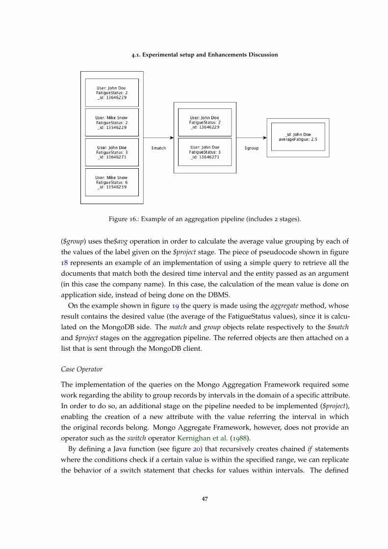
4.1. Experimental setup and Enhancements Discussion

Figure 16.: Example of an aggregation pipeline (includes 2 stages).

($group) uses the$avg operation in order to calculate the average value grouping by each ofthe values of the label given on the $project stage. The piece of pseudocode shown in figure18 represents an example of an implementation of using a simple query to retrieve all thedocuments that match both the desired time interval and the entity passed as an argument(in this case the company name). In this case, the calculation of the mean value is done onapplication side, instead of being done on the DBMS.

On the example shown in figure 19 the query is made using the aggregate method, whoseresult contains the desired value (the average of the FatigueStatus values), since it is calcu-lated on the MongoDB side. The match and group objects relate respectively to the $matchand $project stages on the aggregation pipeline. The referred objects are then attached on alist that is sent through the MongoDB client.

Case Operator

The implementation of the queries on the Mongo Aggregation Framework required somework regarding the ability to group records by intervals in the domain of a specific attribute.In order to do so, an additional stage on the pipeline needed to be implemented ($project),enabling the creation of a new attribute with the value referring the interval in whichthe original records belong. Mongo Aggregate Framework, however, does not provide anoperator such as the switch operator Kernighan et al. (1988).

By defining a Java function (see figure 20) that recursively creates chained if statementswhere the conditions check if a certain value is within the specified range, we can replicatethe behavior of a switch statement that checks for values within intervals. The defined

47

4.1. Experimental setup and Enhancements Discussion

Figure 17.: Example of an aggregation pipeline (includes 3 stages).

Double averageFatigueByCompanyCurrentMonth(String company , String timezone) {

Date date = TimeConverter.getMonthInit(new Date(), timezone)Query <FatigueStatus > query = dataAccessObject.createQuery ()q.field("_id").greaterThanOrEq(new ObjectId(date));q.field("company").equal(company)

List <FatigueStatus > records = q.asList ()

return records.mean()}

Figure 18.: Pseudocode representing the implementation of a simple MongoDB query.

function has as arguments, a list (containing the limits of the filter intervals) and an integerthat specifies the current (on each recursive step) interval conditions being defined.

MongoDB and Storage Engines

To improve writing performance several MongoDB features may be took into account whencustomizing the operating system in the servers that form the replica sets (Tugores andColet (2013)). One of the first considerations is that MongoDB uses write ahead logging toan on-disk journal to guarantee write operation durability and to provide crash resiliency.If the filesystem does not implement journaling and mongod exits unexpectedly the datacan be in an inconsistent state. To avoid this issue ext4 can be used since it implementsjournaling. Besides choosing a convenient filesystem, writing speed can be increased bymounting the file system where the database is located with the option noatime (Zadok

48

4.1. Experimental setup and Enhancements Discussion

Double averageFatigueByCompany(String company , Date init , Date end) {

BasicDBList list = new BasicDBList ()list.add(new BasicDBObject("company", company))list.add(new BasicDBObject("_id", new BasicDBObject("$gt", new ObjectId(

init)))list.add(new BasicDBObject("_id", new BasicDBObject("$lt", new ObjectId(

end)))

BasicDBObject match = new BasicDBObject("$match", new BasicDBObject("$and", list))

BasicDBObject group = new BasicDBObject("$group", new BasicDBObject("_id","$company").append("avg", new BasicDBObject("$avg", "$FatigueLevel")))

List <BasicDBObject > pipeline = new ArrayList <>()pipeline.add(match)pipeline.add(group)

Document output = collection.aggregate(pipeline).first ()return output.getDouble("avg")

}

Figure 19.: Pseudocode representing the implementation of a MongoDB aggregation frameworkquery.

et al. (2015)) avoiding the logging of the record of the last time the file has been accessed ormodified.

Another aspect in the data architecture that must be addressed is related to the storageengines of the DBMS. As the there is no longer a universal database storage technologycapable of powering every type of application built by the business, MongoDB providespluggable storage engines, namely WiredTiger and MMAPv1. Multiple storage enginescan co-exist within a single MongoDB replica set, making it easy to evaluate and migrateengines. Running multiple storage engines within a replica set can also simplify the processof managing the data lifecycle. This approach significantly reduces developer and opera-tional complexity compared to running multiple databases. Therefore, users can leveragethe same MongoDB query language, data model, scaling, security and operational toolingacross different applications, each powered by different pluggable MongoDB storage en-gines. WiredTiger (default storage engine starting in MongoDB 3.2) provides significantbenefits in the areas of lower storage costs, greater hardware utilization, and more pre-dictable performance 3 and, consequently should be used in this system.

3 https://docs.mongodb.org/manual/core/storage-engines/

49

4.1. Experimental setup and Enhancements Discussion

Condition switch (List dates) {Condition condition = new Condition ()

if (dates.size() > 1) {

Interval interval = new Interval("$_id", first(dates), second(dates))condition.if = intervalcondition.then = first(dates)Condition elseCondition = switch(tail(dates))condition.else = elseCondition

} else {

condition.if = "true"condition.then = "Out of bounds."

}return condition

}

Figure 20.: Pseudocode representing the implementation of the case operator.

4.1.2 Caching the queries’ results with EhCache

Additionally to the improvement of the queries’ running time, there was the opportunityfor optimization on application side. The proposed solution was to include a cache forthe queries’ results. A cache can be generally defined as a collection of temporary datathat either duplicates data located elsewhere or is the result of a computation. Data that isalready in the cache can be repeatedly accessed with minimal costs in terms of time andresources. Reducing the response time while also reducing server load were the main goalsof this development stage.

During the analysis of the system there was the opportunity to check the web platform(the data visualization layer) logs, and this enabled the inference of some insights on itsusage. This was the main factor that drove the design of the caching system.

The built cache is part of the Java application (installed using Maven) and was built usingthe Ehcache 4. Alongside with being the most widely-used java cache it is open source, itsupports in-process/out-process (and mixed), and has a Java type-safe API (Ehcache v3).From the provided data (web application logs) the observed number of users regularlylogging on the web application was around one hundred. As it is suggested in ehc thePareto’s law makes a sufficient approach to guess the cache sizes. By defining cache sizesas around 20% of the total query requests (by the Pareto’s law) 80% of the results fromthe queries are expected to be a cache hit (when a data element is requested from cache

4 http://www.ehcache.org

50

4.1. Experimental setup and Enhancements Discussion

and the element exists for the given key). For each cache, there is a similar amount of thestorage allocated off the heap (not subject to garbage collection). These act as a second levelcache (slower response time than first level), that were idealized as useful for values thatare seldom used.

Therefore, by calculating the total number of different queries in a defined amount oftime a guess can be done on how big should be the cache sizes on this early stage ofthe application. Hereupon, there was a final parameter that needed to be tuned on thecaches, the time-to-live (expiration time) of the saved records. According to this, there weredefined two types of caches: the first save the results from queries that need refresh everyfive minutes (such as current hour, current day, current month), and the second save resultsfrom queries that have no expiry time (records are refreshed using a last recently usedpolicy). For each of the two types there are two caches: one for single value results andother for arrays.

An example of the usage of the cache is shown in figure 21 the method. The cache elementis an instance of a singleton object where the caches are defined and initialized.

public double averageFatigueByCompanyCurrentMonth(String company , String tz) {Date initDate = TimeConverter.initMonthDateTz(new Date(), tz);String init = initDate.getTime ().toHexString ();CacheElement cacheElement = new CacheElement(company , initDate.getYear (),

initDate.getMonth ());

if (cache.getDoubleCacheCurrent(cacheElement) != null) {return cache.getDoubleCacheCurrent(cacheElement);

}

Double avg = averageFatigueByCompany(company , init);cache.putDoubleCacheCurrent(cacheElement , avg);return avg;

}

Figure 21.: Example of usage of the defined cache (Java code).

4.1.3 H2O Package

The setup presented on chapter 3 includes a learning algorithm. In order to optimizeperformance and according to what was presented o section 2.4, there was an opportunityfor experimenting with different machine learning libraries in order to improve the classifiertraining performance.

Hereupon, and given the Performetic’s team expertise using the R programming lan-guage and respective environment, there was the preference on using the H2O package

51

4.1. Experimental setup and Enhancements Discussion

(previously introduced) in order to reach the desired goals. Thus, the only change on thesoftware, regarding the deployed version of Performetric’s system, was made in the coderespective to the training of the classifier.

For this experimental procedure the number of rows in the provided dataset is 10000.The dataset was initially split in two, generating the training dataset (by including 75% ofthe original rows, randomly selected) and the testing dataset (by including the remaining25% of the original rows). This was the selected option for results validation, in oppositionto, for example, cross-validation.

The H2O packages features a deep neural network API that enable the easy deploymentof a classifier based on this kind of algorithms. The R code respective to the definition ofthe neural network is shown on figure 22.

predictors <- c( ’Performance.KDTMean ’, ’Performance.MAMean ’, ’Performance.MVMean ’, ’Performance.TBCMean ’, ’Performance.DDCMean ’, ’Performance.DMSLean ’, ’Performance.AEDMean ’, ’Performance.ADMSLMean ’)

net <- h2o.deeplearning(training_frame=trainset ,x=predictors ,y=’FatigueLevel ’,activation="Rectifier",hidden = c(40 ,25),epochs = 500

)

Figure 22.: Example of usage of neural networks with H2O (R code).

The training frame, x and y parameters refer to the selection of the dataset, the namingof the features and the definition of the label feature, respectively. As for the rest of theparameters:

ACTIVATION A string indicating the activation function to use. Must be either “Tanh”, “Tan-hWithDropout”, “Rectifier”, “RectifierWithDropout”, “Maxout”, or “MaxoutWithDropout”

HIDDEN The schema of the hidden layers in the neural network.

EPOCHS How many times the dataset should be iterated (streamed).

These parameters have been optimized using the grid search hyper-parameter tuningincluded in H2O. The machine where the tests were run has the same specifications as themachines that were used in the experiments regarding query optimization (see subsection4.2.1). As for the results, beyond the running time, were recorded the values for the root-

52

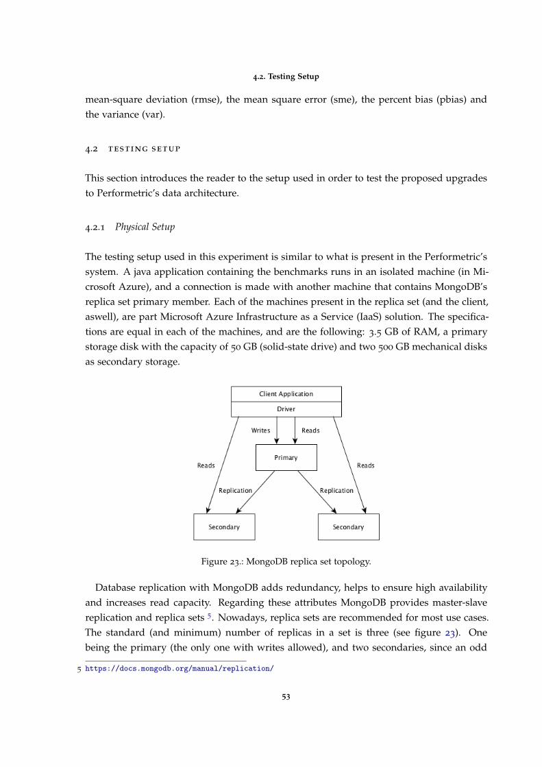
4.2. Testing Setup

mean-square deviation (rmse), the mean square error (sme), the percent bias (pbias) andthe variance (var).

4.2 testing setup

This section introduces the reader to the setup used in order to test the proposed upgradesto Performetric’s data architecture.

4.2.1 Physical Setup

The testing setup used in this experiment is similar to what is present in the Performetric’ssystem. A java application containing the benchmarks runs in an isolated machine (in Mi-crosoft Azure), and a connection is made with another machine that contains MongoDB’sreplica set primary member. Each of the machines present in the replica set (and the client,aswell), are part Microsoft Azure Infrastructure as a Service (IaaS) solution. The specifica-tions are equal in each of the machines, and are the following: 3.5 GB of RAM, a primarystorage disk with the capacity of 50 GB (solid-state drive) and two 500 GB mechanical disksas secondary storage.

Figure 23.: MongoDB replica set topology.

Database replication with MongoDB adds redundancy, helps to ensure high availabilityand increases read capacity. Regarding these attributes MongoDB provides master-slavereplication and replica sets 5. Nowadays, replica sets are recommended for most use cases.The standard (and minimum) number of replicas in a set is three (see figure 23). Onebeing the primary (the only one with writes allowed), and two secondaries, since an odd

5 https://docs.mongodb.org/manual/replication/

53

4.2. Testing Setup

number of members ensures that the replica set is always able to elect a primary. Whenever,the primary becomes unavailable, an election is triggered selecting one of the remainingsecondaries as the new primary (see figure 24). The setup used in this experiment includesa three-member replica set.

Figure 24.: MongoDB replica set topology (after primary member becomes unavailable).

Each of the machines in the presented set runs a LTS version of Ubuntu (14.04) and arepart of the same network (an option provided by Microsoft Azure), have MongoDB 3.0version and have the Java SE Development Kit 8 (JDK 8) installed.

4.2.2 Data Collection

In order to make accurate measurements that may lead to an effective analysis of the timeelapsed during the data processing, a set of benchmarks was setup using the JMH - Java Mi-crobenchmark Harness toolkit. For a the set of methods defined in the QueryListInterfaceinterface, three classes were coded containing, respectively, the code related to the existingsolution, the solution using Mongo Aggregation Framework, and the solution that savesresults of a query in a cache. An example of usage of JMH is provided in figure 25.

The mode and the precision (different orders of magnitude, such as nanoseconds, mi-croseconds, milliseconds and seconds) of the measurements can be specified for each bench-mark. In the presented example the time unit is nanoseconds and the mode is SimpleTime.The set of modes available in JMH are presented below:

THROUGHPUT Measures the number of operations per second, meaning the number oftimes per second your benchmark method could be executed.

AVERAGE TIME Measures the average time it takes for the benchmark method to execute (asingle execution).

54

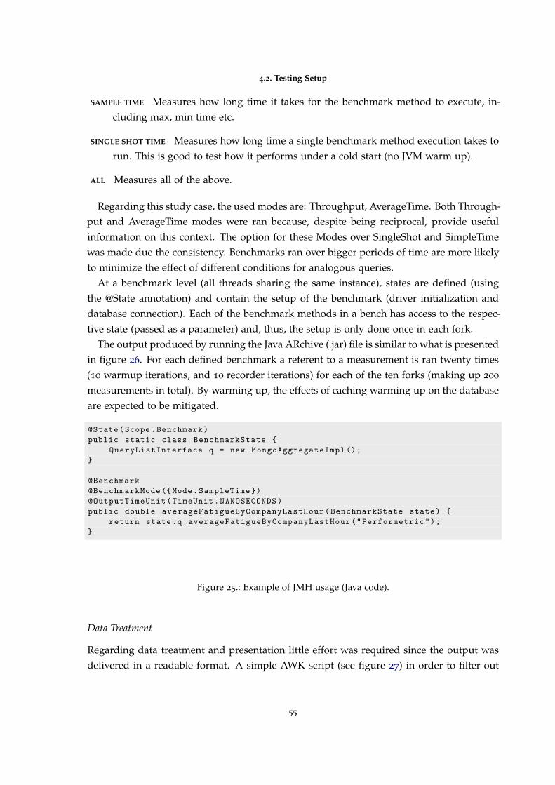
4.2. Testing Setup

SAMPLE TIME Measures how long time it takes for the benchmark method to execute, in-cluding max, min time etc.

SINGLE SHOT TIME Measures how long time a single benchmark method execution takes torun. This is good to test how it performs under a cold start (no JVM warm up).

ALL Measures all of the above.

Regarding this study case, the used modes are: Throughput, AverageTime. Both Through-put and AverageTime modes were ran because, despite being reciprocal, provide usefulinformation on this context. The option for these Modes over SingleShot and SimpleTimewas made due the consistency. Benchmarks ran over bigger periods of time are more likelyto minimize the effect of different conditions for analogous queries.

At a benchmark level (all threads sharing the same instance), states are defined (usingthe @State annotation) and contain the setup of the benchmark (driver initialization anddatabase connection). Each of the benchmark methods in a bench has access to the respec-tive state (passed as a parameter) and, thus, the setup is only done once in each fork.

The output produced by running the Java ARchive (.jar) file is similar to what is presentedin figure 26. For each defined benchmark a referent to a measurement is ran twenty times(10 warmup iterations, and 10 recorder iterations) for each of the ten forks (making up 200

measurements in total). By warming up, the effects of caching warming up on the databaseare expected to be mitigated.

@State(Scope.Benchmark)public static class BenchmarkState {

QueryListInterface q = new MongoAggregateImpl ();}

@Benchmark@BenchmarkMode ({Mode.SampleTime })@OutputTimeUnit(TimeUnit.NANOSECONDS)public double averageFatigueByCompanyLastHour(BenchmarkState state) {

return state.q.averageFatigueByCompanyLastHour("Performetric");}

Figure 25.: Example of JMH usage (Java code).

Data Treatment

Regarding data treatment and presentation little effort was required since the output wasdelivered in a readable format. A simple AWK script (see figure 27) in order to filter out

55

4.2. Testing Setup

# Run progress: 0.81% complete , ETA 13:20:38

# Fork: 10 of 10

# Warmup Iteration 1: 2016 -03 -11 16:15:55 INFO cluster :71 - Cluster created

with settings {hosts =[ maindb.cloudapp.net :27017] , mode=SINGLE ,

requiredClusterType=UNKNOWN , serverSelectionTimeout = ’30000 ms’,

maxWaitQueueSize =60000}

# Warmup Iteration 1: 0.610 ops/s

# Warmup Iteration 2: 7.437 ops/s

# Warmup Iteration 3: 8.531 ops/s

# Warmup Iteration 4: 8.361 ops/s

# Warmup Iteration 5: 8.977 ops/s

# Warmup Iteration 6: 9.627 ops/s

# Warmup Iteration 7: 9.429 ops/s

# Warmup Iteration 8: 9.436 ops/s

# Warmup Iteration 9: 9.577 ops/s

# Warmup Iteration 10: 9.509 ops/s

Iteration 1: 9.827 ops/sIteration 2: 10.092 ops/sIteration 3: 9.908 ops/sIteration 4: 9.930 ops/sIteration 5: 9.557 ops/sIteration 6: 9.976 ops/sIteration 7: 9.467 ops/sIteration 8: 9.792 ops/sIteration 9: 9.709 ops/sIteration 10: 10.036 ops/s

Figure 26.: Example of output generated by JMH benchmarks.

the summarized results. Additionally the features provided by Sublime Text enabled theconversion of the data to LATEXtables and diagrams.

56

4.3. Results

{if ($0 ~ "# Benchmark mode:") print $0;if ($0 ~ "# Benchmark:") print $0;if ($0 ~ "Result:") print $0;if ($0 ~ "Statistics:") print $0;if ($0 ~ "Confidence interval") print $0 "\n";

}

Figure 27.: Piece of AWK code used for parsing the output generated by JMH.

4.3 results

In this section the results obtained are shown to the reader. In each subsection, the perfor-mance results of different parts of the system are presented. Whenever it is appropriate acomparison between the existing and proposed solution is shown.

57

4.3. Results

4.3.1 Data Aggregation

In the following set of figures, the results of the tests ran on the queries (see subsection3.2.1 for the list of queries) are plotted. As it was mentioned on subsection 4.2.2 the chosenmodes were Throughput and Average Time. The thorughput is measured over a period ofone second, as for the average time is calculated based on a set of 200 samples for eachbenchmark.

For each of the queries, the average times and the measured throughput of the currentimplementation are shown side-by-side with the results of the implementation that usesMongoDB aggregate. The goal is to provide insight on how the performance changedafter the proposed enhancements. For each graph, the respective values can be consultedon Appendix A in sections related to each of the topics in this subsection. The results ofqueries for which the granularity of the time filter is the hour are shown on section A.5.This set of plots shows that results are fairly similar and were isolated because the intervalsare much smaller than the others (day, week, month).

In the figures 28 and 29 are shown the results of the benchmarks ran on the queries thatfilter the results by a company name. Each of the queries in this set returns a double valueresulting of the filtering the Fatigue Status collection by a time interval (specified in labelspresented on the charts) and subsequent calculation the respective average value. The firstpair of charts (see figure 28) shows the results for the queries for open intervals (filters dataonly by the beginning of the interval). As for figure 29 is shows the results for querieswhere the filtered documents are inside a closed interval (between the beginning and endof the respective time span).

The same presentation pattern is followed for the queries that filter the Fatigue Statuscollection by team name (see figures 30 and 31) and by user name (see figures 32 and 33).

58

4.3. Results

Company Queries Execution Performance

Day Week Month0

200

400

600

800 771.55 740.54 742.6

852.05 823.4 787.98

Ave

rage

time

(us/

op)

Day Week Month0

2

4

6

8

109.98

2.781.59

10.29

4.913.72

Thro

ughp

ut(o

ps/s

)

JavaMongoDB

Figure 28.: Comparison between Java and MongoDB aggregation framework implementations(queries about a specific company name) for a current time interval (see subsection 3.2.1).

Day Week Month0

2

4

6

·104

760.28 999.06

62,500.96

885.33 911.76

28,666.48

Ave

rage

time

(us/

op)

Day Week Month0

2

4

6

8

10 9.45

6.81

2.2

10.46

7

2.61

Thro

ughp

ut(o

ps/s

)

JavaMongoDB

Figure 29.: Comparison between Java and MongoDB aggregation framework implementations(queries about a specific company name) for a past time interval (see subsection 3.2.1).

59

4.3. Results

Team Queries Execution Performance

Day Week Month0

200

400

600

800 779.51 779.27 772.28829

888.92 892.37

Ave

rage

time

(us/

op)

Day Week Month0

5

10

15

2020.6

6.414.33

14.74

5.314Th

roug

hput

(ops

/s)

JavaMongoDB

Figure 30.: Comparison between Java and MongoDB aggregation framework implementations(queries about a specific team name) for a current time interval (see subsection 3.2.1).

Day Week Month0

0.5

1

1.5

2

2.5

·104

808.22 835.17

16,660.24

922.92 910.69

25,852.14

Ave

rage

time

(us/

op)

Day Week Month0

2

4

6

8

10 9.45

6.81

2.2

10.46

7

2.61

Thro

ughp

ut(o

ps/s

)

JavaMongoDB

Figure 31.: Comparison between Java and MongoDB aggregation framework implementations(queries about a specific team name) for a past time interval (see subsection 3.2.1).

60

4.3. Results

User Queries Execution Performance

Day Week Month0

200

400

600

800 756.21 743.26 754.37835.95 855.61 867.6

Ave

rage

time

(us/

op)

Day Week Month0

5

10

15

20

25

19.75

7.315.61

23.98

5.754.44Th

roug

hput

(ops

/s)

JavaMongoDB

Figure 32.: Comparison between Java and MongoDB aggregation framework implementations(queries about a specific user name) for a current time interval (see subsection 3.2.1).

Day Week Month0

0.5

1

1.5

2

·104

797.8 778.33

14,622.37

892.8 837.43

20,699.2

Ave

rage

time

(us/

op)

Day Week Month0

5

10

15

20 19.83

8.13

3.34

10.57

7.64

3.2Thro

ughp

ut(o

ps/s

)

JavaMongoDB

Figure 33.: Comparison between Java and MongoDB aggregation framework implementations(queries about a specific user name) for a past time interval (see subsection 3.2.1).

Group By Queries Execution Performance

Each of the following pair of charts refers to a set of queries that groups the Fatigue Statusby time intervals, according to the granularity specified by the labels in the charts. Thisset of queries follows the structure presented on figure 17 and each one returns arrays ofdoubles.

The values associated with the label Day refer to the queries that calculate the averagevalue for each hour given a day and an entity (user, team and/or company names). As

61

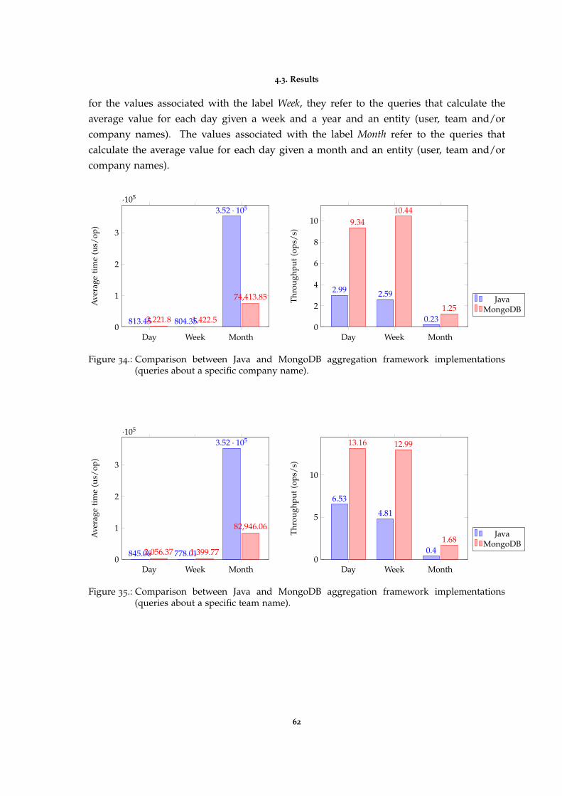
4.3. Results

for the values associated with the label Week, they refer to the queries that calculate theaverage value for each day given a week and a year and an entity (user, team and/orcompany names). The values associated with the label Month refer to the queries thatcalculate the average value for each day given a month and an entity (user, team and/orcompany names).

Day Week Month0

1

2

3

·105

813.45 804.35

3.52 · 105

2,221.8 1,422.5

74,413.85

Ave

rage

time

(us/

op)

Day Week Month0

2

4

6

8

10

2.99 2.59

0.23

9.3410.44

1.25

Thro

ughp

ut(o

ps/s

)Java

MongoDB

Figure 34.: Comparison between Java and MongoDB aggregation framework implementations(queries about a specific company name).

Day Week Month0

1

2

3

·105

845.06 778.01

3.52 · 105

2,056.37 1,399.77

82,946.06

Ave

rage

time

(us/

op)

Day Week Month0

5

10

6.53

4.81

0.4

13.16 12.99

1.68

Thro

ughp

ut(o

ps/s

)

JavaMongoDB

Figure 35.: Comparison between Java and MongoDB aggregation framework implementations(queries about a specific team name).

62

4.3. Results

Day Week Month0

1

2

3

·105

795.23 753.49

3.48 · 105

2,033 1,481.11

73,618.6

Ave

rage

time

(us/

op)

Day Week Month0

5

10

15

6.71

8.72

0.46

14.95 15.61

2.1

Thro

ughp

ut(o

ps/s

)

JavaMongoDB

Figure 36.: Comparison between Java and MongoDB aggregation framework implementations(queries about a specific user name).

Cache Performance

The results of the performance evaluation on the Cache can be examined in section A.6.As it would be expected the results are not on the same order of magnitude of the onespresented in section the previous sections. As can be observed the results of the averagetime for accessing the cache in the mounted setup are around the microseconds per opera-tion, which is considerably less than the running time of the queries. As for the throughputit is roughly around the 1e5 operations per second, which (as expected) is much higherthan the throughput obtained when running the queries, independently of the usage of theMongoDB Aggregation Framework.

The set of queries in which the time interval is one or two hours before the time whenthe request is made are excluded form this set of results as its caching is unnecessary sincethis values are frequently updated and cached on client applications.

4.3.2 Data Classification

The following table (see table 4) shows the results obtained in the experiment involvingthe classifier training. The set of values for the four selected metrics (the root-mean-squaredeviation, the mean square error, the percent bias and the variance) are shown side-by-side,as well as the training time, for each of the implementations (R neuralnet package, and h2opackage).

The values under NeuralNet Package column refer to the optimized parameters, obtainedby Performetric. These values were obtained through GridSearch (Bergstra and Bengio(2012)). The parameters optimized were: the configuration of the two hidden layers in the

63

4.3. Results

network (the obtained value was 40 nodes on the first hidden layer and 25 nodes in thesecond hidden layer), the threshold for the partial derivatives of the error function (on thestopping criteria, the obtained value was 0.01) and the maximum steps for the training ofthe neural network (another stopping criteria, the obtained value was 2e09).

NeuralNet Package H2O implementationRMSE 2.067289212 1.48904

MSE 4.273684685 2.21724

PBIAS (%) -6.4 11.9VAR 0.8397328191 -0.01441812

Time (seconds) 232.39 24.825

Table 4.: Classifier training results.

64

4.4. Summary

4.4 summary

This chapter introduces the reader to the setup used in the experiments. The importantand unique aspects of the setup are described. Additionally, the testing methodology ispresented along with the obtained results. Some additional details are included in order togive helpful hints to those who work with this or similar systems in the future.

The decisions behind the proposed enhancements are hereby introduced and justified.The results are presented in a coeherent form, enabling a simple comparision between thecurrent solutions and the proposed upgrades. All the results that may introduce noise inthe analysis are sent to the appendixes and refered in this chapter.

65

5

R E S U LT A N A LY S I S A N D D I S C U S S I O N

In this chapter the results obtained in the experiments presented on the previous chapterwill be analyzed. Whenever possible, conclusions and explanations about the observationswill be provided. Each section refers to each of the different experiments. For each topicthe results are discussed and criticized, and whenever possible conclusions are inferred.

5.1 data aggregation

For analysis purposes, this part of the results can be divided in three parts: the performanceresults for the simpler queries (whose pipeline consists in two stages, see figure 16 onchapter 4), the performance results for more complex queries (whose pipeline consists intwo stages, see figure 17 on chapter 4) and the performance results for the caching system.

5.1.1 Simple queries results analysis

The set of figures that include the ones from figure 28 to figure 33, is related to this type ofqueries.

As it can be seen (and as it would be expected) there are similarities on the graphs thatplot the average time (per day, week and month) for the company, team and user for acurrent time interval. It is shown an increase in the average time on the order of the 100

microseconds (from around 700 microseconds average to around 800 microseconds).As for the respective throughput, the values for the Mongo Aggregate are very similar in

the three graphs, and there is a trend (except in the company queries) that shows a decreasein the throughput values (that is consistent with the average time values).

Regarding the graphs for past intervals, the values of both the average times and thethroughput are consistent for the implementation that uses the Mongo Aggregate. As forthe values for the Java implementation are not consistent across company, team and userplots, the task of drawing conclusions becomes more difficult. There is no clear trend, but

66

5.1. Data Aggregation

generally, the results are worse than in the Java implementation (bigger average responsetimes, and smaller throughput values).

Behind the incoherence on the values, may be the fact that the Java implementationmay not follow the same structure across similar methods, as opposed to what happensin the Mongo Aggregate implementation. Another possible reason, is that the overhead ofusing the Mongo Aggregate may do not pay off for queries of this complexity (relativelysimple) and its benefits may not be shown in this setup. The obtained results are measuredfor the whole operation, the only way for comparing the performance between the twoimplementations.

Despite having benefits, as the amount of data that is transferred between machines inthe Mongo Aggregate implementation is smaller (computations are made on the DBMS, inopposition to the Java implementation), there are no evidences that the proposed imple-mentation would perform better in this case.

5.1.2 Complex queries results analysis

The set of figures that include the ones from figure 34 to figure 36, is related to this type ofqueries.

The results are very similar across company, team and user. There is a general trend forthe improvement of the performance, both the average times and the respective throughput,in the Mongo Aggregate implementation (in opposition to the Java implementation).

It must be noted, though, that as the granularity of the time interval increases the benefitsgrow bigger. The relative improvements (the proportion between the previous and therecent implementations results) are higher in the month than the ones observed in the week,and in turn, the relative improvements in the week results are higher that ones observed inthe day.

The benefits of using Mongo Aggregation Framework for this type of queries are tangible.Thus, it should be implemented on Performetric’s system.

5.1.3 Caching queries results analysis

As it was noted in the subsection 4.3.1 the average times of accessing the caches are smaller(in several orders of magnitude) and the throughput is much higher. Implementing a cachein this system must be done at this level (as opposed to a cache for the web pages, for exam-ple) as, for example, a decision agent may consult data that has already been summarized,from another machine.

Despite increasing the complexity on the application development, the decision of inte-grating the cache in the Performetric system should be made, as the benefits are evident.

67

5.2. Data Classification

5.2 data classification

This experiment led to a comparison between the performance in both speed and accuracybetween a R native implementation and the implementation provided by H2O. Each of thestatistical measure is computed between the values obtained by the respective classifier andthe values that were expected (values range from 1 to 7, accoring to the mental fatigue scalecreated in about 1979 by Dr. William F. Storm and Captain Layne P. Perelli of the CrewPerformance Branch of the USAF School of Aerospace Medicine, Brooks AFB, San Antonio,Texas, Samn and Perelli (1982)). The obtained results are shown on table 4.

The value obtained for the root-mean-square deviation (RMSE) decreased relatively tothe previous implementation (2.0673 to 1.4890, as it is expected the mean square error -MSE - value also decreased, 4.2736 to 2.2172). This parameter gives the standard deviationof the model prediction error. A smaller value indicates a better model performance.

The percent bias (PBIAS) measures the average tendency of the simulated values to belarger or smaller than their observed ones. The optimal value of PBIAS is 0.0, with low-magnitude values indicating accurate model simulation. Positive values indicate overesti-mation bias, whereas negative values indicate model underestimation bias (the results aregiven in percentage). The value obtained for the R implementation is better (-6.4) than theobtained on the H2O implementation (11.9).

The variance measures how far each number in the set is from the mean. A variance valueof zero indicates that all values within the set are identical. A large variance indicates thatnumbers in the set are far from the mean and each other, while a small variance indicatesthe opposite. In this case, as the variance values vary from 0.8397328191 to -0.01441812,it can be observed that the there was an improvement in this measure. The differencebetween the obtained and expected results is smaller for each record, generally, in the H2Oimplementation.

The speed of the training is the measure where the results are more clear. The trainingon R implementation ran on 232.39 seconds, and the H2O implementation ran on 24.825

seconds, which means a value around ten times smaller.As it is commonly referred in data mining literature, more data could mean more reliable

results. Another way to make the results be more reliable is to use cross-validation insteadof traditional validation for assessing the results.

By experimenting with deeper configurations of the neural networks (which H2O sup-ports), it may be possible to improve the accuracy of the model. Although it can be arguedagainst the improvement of the performance of the classifier, there is a clear improvementon speed of the training. The training speed is vital to the system, and the main focus inthis work, so it can be said it there was an improvement, regarding the defined goals.

68

5.3. Project Execution Overview

5.3 project execution overview

Regarding what was initially planned the way the development of this project went sufferedsome deviations. The study of ways to improve the classifier was not in the initial plans forthis thesis, but as it is such a big concert on this architecture it was imperative that it wasaddressed.

As it can be noted there were no tests on possible optimizations regarding data insertion,however the techniques for doing so are well described on MongoDB documentation andits benefits are proven (and as it was previously presented, when applied on early stages ofthe application may even degrade performance).

Despite not all the results being positive (as it is addressed in subsection 5.1.1) the set oftested hypotheses provide helpful insights on how the system can be improved.

69

6

C O N C L U S I O N

This final chapter has the objective of providing a comprehensive synthesis of all the workthat has been accomplished along with the findings that were drawn from the results ob-tained. Additionally, some insight will be given into the future work that could be done inthe pursuit of better results.

6.1 work synthesis

Keeping a performing system in a cutting edge field as it is Performetric’s, is an hardtask. The crossing between Big Data, Machine Learning and Internet of Things field hasbrings lots of opportunities and challenges, that are addressed everyday in both academicand industrial environments. However, the presented work is a step forward in what itis expected to be a successful large-scale software solution for providing monitoring onmental fatigue and, ultimately, wellness. By tackling some issues on the data architectureof the company some contributions have been made, and hopefully can be replicated insimilar contexts.

The first achieved goal of this work was to carry a study on Big Data (and document itas a state-of-the-art), this helped to frame the problem. The next step was to produce thearchitecture documentation for the Performetric system. This enabled the gathering of thecontextual needs. The development of the testing setup, the prototypes and the measuringmechanisms, was a goal that was achieved. The development of this task led to the arisingof artifacts (queries’ code, the caching system code, the H2O code) that may be includedin the deployed system. The analysis of the obtained results makes this contribution marevaluable, as the results are expected to be replicated in similar contexts.

As an additional result, from this work resulted the following publication: Araujo D.,Pimenta A., Carneiro D., Novais P., Providing Wellness Services Using Real Time Analytics,Ambient Intelligence- Software and Applications – 7th International Symposium on Ambi-ent Intelligence (ISAmI 2016), Springer - Advances in Intelligent Systems and Computing,

70

6.2. Prospect for future work

Lindgren H. et al. (eds), Vol 476, ISSN 2194-5357, ISBN 9783319401133, pp 167-175, 2016.http://dx.doi.org/10.1007/978-3-319-40114-0_19.

6.2 prospect for future work

Despite reaching successfully all the defined goals, this study is not nearly over. The op-portunities to experiment with the system and for tuning it are huge. There are somesuggested improvements that may be followed in order to increase the system performanceand robustness. The first suggestion presented in section 3.2.2 of using a sharded clusterand a messaging queue in order to handle data insertion and increase availability.

The study on the classifier training was limited and mainly focused on speed of the train-ing. However, there are many opportunities for optimization in this topic. The deploymentof a continuous learning system should be on the roadmap. Additionally, the emerging ofdeep learning frameworks such as the ones presented in the literature review section of thisdocument should not be neglected.

On the other hand, there are unexplored opportunities that share the context with Perfor-metric, namely the use of different non-intrusive devices (such as wrist trackers or smart-phones), that may constitute interesting challenges on the tasks of data-handling.

71

B I B L I O G R A P H Y

About ehcache, version 2.9. http://www.ehcache.org/generated/2.9.0/pdf/About_

Ehcache.pdf. (Accessed on 20/04/2016).

Martın Abadi, Ashish Agarwal, Paul Barham, Eugene Brevdo, Zhifeng Chen, Craig Citro,Greg S Corrado, Andy Davis, Jeffrey Dean, Matthieu Devin, et al. Tensorflow: Large-scalemachine learning on heterogeneous distributed systems. arXiv preprint arXiv:1603.04467,2016.

A. Aggarwal. Managing Big Data Integration in the Public Sector. Advances in Public Pol-icy and Administration:. 2015. ISBN 9781466696501. URL https://books.google.com/

books?id=EgHqCgAAQBAJ.

Anisha Arora, Arno Candel, Jessica Lanford, Erin LeDell, and Viraj Parmar. Deep learningwith h2o, 2015.

Marcos D Assuncao, Rodrigo N Calheiros, Silvia Bianchi, Marco AS Netto, and RajkumarBuyya. Big data computing and clouds: Trends and future directions. Journal of Paralleland Distributed Computing, 79:3–15, 2015.

AM Bagirov, AM Rubinov, NV Soukhoroukova, and J Yearwood. Unsupervised and super-vised data classification via nonsmooth and global optimization. Top, 11(1):1–75, 2003.

Soheil Bahrampour, Naveen Ramakrishnan, Lukas Schott, and Mohak Shah. Comparativestudy of caffe, neon, theano, and torch for deep learning. arXiv preprint arXiv:1511.06435,2015.

Len Bass, Paul Clements, and Rick Kazman. Software architecture in practice. 2012.

R Bellman. Curse of dimensionality. Adaptive control processes: a guided tour. Princeton, NJ,1961.

James Bergstra and Yoshua Bengio. Random search for hyper-parameter optimization. TheJournal of Machine Learning Research, 13(1):281–305, 2012.

James Bergstra, Frederic Bastien, Olivier Breuleux, Pascal Lamblin, Razvan Pascanu, OlivierDelalleau, Guillaume Desjardins, David Warde-Farley, Ian Goodfellow, Arnaud Bergeron,et al. Theano: Deep learning on gpus with python. In NIPS 2011, BigLearning Workshop,Granada, Spain, 2011.

72

Bibliography

Elisa Bertino, Philip Bernstein, Divyakant Agrawal, Susan Davidson, Umeshwas Dayal,Michael Franklin, Johannes Gehrke, Laura Haas, Alon Halevy, Jiawei Han, et al. Chal-lenges and opportunities with big data. 2011.

Peter Buneman. Semistructured data. In Proceedings of the sixteenth ACM SIGACT-SIGMOD-SIGART symposium on Principles of database systems, pages 117–121. ACM, 1997.

Davide Carneiro, Ricardo Costa, Paulo Novais, Joao Neves, J Machado, and Jose Neves.Simulating and monitoring ambient assisted living. In Proceedings of the ESM, pages 175–182, 2008.

Davide Carneiro, Jose Carlos Castillo, Paulo Novais, Antonio Fernandez-Caballero, andJose Neves. Multimodal behavioral analysis for non-invasive stress detection. ExpertSystems with Applications, 39(18):13376–13389, 2012.

Davide Carneiro, Andre Pimenta, Sergio Goncalves, Jose Neves, and Paulo Novais. Mon-itoring and improving performance in human–computer interaction. Concurrency andComputation: Practice and Experience, 28(4):1291–1309, 2016. ISSN 1532-0634. doi:10.1002/cpe.3635. URL http://dx.doi.org/10.1002/cpe.3635. cpe.3635.

Rick Cattell. Scalable sql and nosql data stores. ACM SIGMOD Record, 39(4):12–27, 2011.

Fay Chang, Jeffrey Dean, Sanjay Ghemawat, Wilson C Hsieh, Deborah A Wallach, MikeBurrows, Tushar Chandra, Andrew Fikes, and Robert E Gruber. Bigtable: A distributedstorage system for structured data. ACM Transactions on Computer Systems (TOCS), 26(2):4, 2008.

Surajit Chaudhuri and Umeshwar Dayal. An overview of data warehousing and olap tech-nology. ACM Sigmod record, 26(1):65–74, 1997.

Min Chen, Shiwen Mao, and Yunhao Liu. Big data: A survey. Mobile Networks and Applica-tions, 19(2):171–209, 2014.

Peter Pin-Shan Chen. The entity-relationship model—toward a unified view of data. ACMTransactions on Database Systems (TODS), 1(1):9–36, 1976.

Michael Chui, Markus Loffler, and Roger Roberts. The internet of things. McKinsey Quar-terly, 2(2010):1–9, 2010.

Paul Clements, David Garlan, Len Bass, Judith Stafford, Robert Nord, James Ivers, andReed Little. Documenting software architectures: views and beyond. Pearson Education, 2002.

Alfredo Cuzzocrea, Il-Yeol Song, and Karen C Davis. Analytics over large-scale multidimen-sional data: the big data revolution! In Proceedings of the ACM 14th international workshopon Data Warehousing and OLAP, pages 101–104. ACM, 2011.

73

Bibliography

Li Da Xu, Wu He, and Shancang Li. Internet of things in industries: A survey. IndustrialInformatics, IEEE Transactions on, 10(4):2233–2243, 2014.

Jeffrey Dean and Sanjay Ghemawat. Mapreduce: simplified data processing on large clus-ters. Communications of the ACM, 51(1):107–113, 2008.

Terrance J Dishongh, Michael McGrath, and Ben Kuris. Wireless sensor networks for healthcareapplications. Artech House, 2014.

Pedro Domingos. A few useful things to know about machine learning. Communications ofthe ACM, 55(10):78–87, 2012.

Brad Fitzpatrick. Distributed caching with memcached. Linux journal, 2004(124):5, 2004.

Apache Software Foundation. Technical overview of apache couchdb. 2014. URL http:

//wiki.apache.org/couchdb/TechnicalOverview.

John Gantz and David Reinsel. Extracting value from chaos. IDC iview, (1142):9–10, 2011.

Gartner. What is big data? http://www.gartner.com/it-glossary/big-data. Accessed:2015-12-20.

M Gentili and PB Mirchandani. Locating sensors on traffic networks: Models, challengesand research opportunities. Transportation research part C: emerging technologies, 24:227–255,2012.

Seth Gilbert and Nancy Lynch. Brewer’s conjecture and the feasibility of consistent, avail-able, partition-tolerant web services. ACM SIGACT News, 33(2):51–59, 2002.

M. Gualtieri and R. Curran. The forrester wave: Big data streaming analytics platforms, q3

2014. 2014.

IBM. The four v’s of big data. http://www.ibmbigdatahub.com/infographic/

four-vs-big-data. Accessed: 2015-12-20.

Jithin Jose, Hari Subramoni, Miao Luo, Minjia Zhang, Jian Huang, Md Wasi-ur Rahman,Nusrat S Islam, Xiangyong Ouyang, Hao Wang, Sayantan Sur, et al. Memcached de-sign on high performance rdma capable interconnects. In Parallel Processing (ICPP), 2011International Conference on, pages 743–752. IEEE, 2011.

Miltiadis Kandias, Vasilis Stavrou, Nick Bozovic, Lilian Mitrou, and Dimitris Gritzalis. Canwe trust this user? predicting insider’s attitude via youtube usage profiling. In UbiquitousIntelligence and Computing, 2013 IEEE 10th International Conference on and 10th InternationalConference on Autonomic and Trusted Computing (UIC/ATC), pages 347–354. IEEE, 2013.

74

Bibliography

Arun Kejariwal, Sanjeev Kulkarni, and Karthik Ramasamy. Real time analytics: algorithmsand systems. Proceedings of the VLDB Endowment, 8(12):2040–2041, 2015.

Brian W Kernighan, Dennis M Ritchie, and Per Ejeklint. The C programming language, vol-ume 2. prentice-Hall Englewood Cliffs, 1988.

Hamzeh Khazaei, Marios Fokaefs, Saeed Zareian, Nasim Beigi-Mohammadi, Brian Ram-prasad, Mark Shtern, Purwa Gaikwad, and Marin Litoiu. How do i choose the rightnosql solution? a comprehensive theoretical and experimental survey. Submitted to Jour-nal of Big Data and Information Analytics (BDIA), 2015.

Hanjoo Kim, Jaehong Park, Jaehee Jang, and Sungroh Yoon. Deepspark: Spark-baseddeep learning supporting asynchronous updates and caffe compatibility. arXiv preprintarXiv:1602.08191, 2016.

Yann LeCun, Yoshua Bengio, and Geoffrey Hinton. Deep learning. Nature, 521(7553):436–444, 2015.

Kyong-Ha Lee, Yoon-Joon Lee, Hyunsik Choi, Yon Dohn Chung, and Bongki Moon. Paralleldata processing with mapreduce: a survey. AcM sIGMoD Record, 40(4):11–20, 2012.

Joao Ricardo Lourenco, Bruno Cabral, Paulo Carreiro, Marco Vieira, and Jorge Bernardino.Choosing the right nosql database for the job: a quality attribute evaluation. Journal ofBig Data, 2(1):1–26, 2015.

Jonathan I Maletic and Andrian Marcus. Data cleansing: Beyond integrity analysis. In IQ,pages 200–209. Citeseer, 2000.

James Manyika, Michael Chui, Brad Brown, Jacques Bughin, Richard Dobbs, Charles Rox-burgh, and Angela H Byers. Big data: The next frontier for innovation, competition, andproductivity. 2011.

Viktor Mayer-Schonberger and Kenneth Cukier. Big data: A revolution that will transform howwe live, work, and think. Houghton Mifflin Harcourt, 2013.

Andrew Kachites McCallum. Reinforcement learning with selective perception and hidden state.PhD thesis, University of Rochester, 1996.

Thomas M Mitchell. Machine learning. Machine Learning, 1997.

D Nelubin and B Engber. Nosql failover characteristics: Aerospike, cassandra, couchbase,mongodb. Thumbtack Technology, 2013.

Alex Sandy Pentland. The data-driven society. Scientific American, 309(4):78–83, 2013.

75

Bibliography

Andre Pimenta, Davide Carneiro, Paulo Novais, and Jose Neves. Monitoring mental fatiguethrough the analysis of keyboard and mouse interaction patterns. In Hybrid ArtificialIntelligent Systems, pages 222–231. Springer, 2013.

Andre Pimenta, Davide Carneiro, Paulo Novais, and Jose Neves. Analysis of Human Per-formance as a Measure of Mental Fatigue, pages 389–401. Springer International Publish-ing, Cham, 2014. ISBN 978-3-319-07617-1. doi: 10.1007/978-3-319-07617-1 35. URLhttp://dx.doi.org/10.1007/978-3-319-07617-1_35.

Andre Pimenta, Davide Carneiro, Jose Neves, and Paulo Novais. Improving User Privacy andthe Accuracy of User Identification in Behavioral Biometrics, pages 15–26. Springer Interna-tional Publishing, Cham, 2015. ISBN 978-3-319-23485-4. doi: 10.1007/978-3-319-23485-4 2.URL http://dx.doi.org/10.1007/978-3-319-23485-4_2.

Andre Pimenta, Davide Carneiro, Jose Neves, and Paulo Novais. A neural network toclassify fatigue from human–computer interaction. Neurocomputing, 172:413–426, 2016.

Dan Pritchett. Base: An acid alternative. Queue, 6(3):48–55, 2008.

Raul Rojas. Neural networks: a systematic introduction. Springer Science & Business Media,2013.

Luis Ruiz-Garcia, Loredana Lunadei, Pilar Barreiro, and Ignacio Robla. A review of wirelesssensor technologies and applications in agriculture and food industry: state of the art andcurrent trends. Sensors, 9(6):4728–4750, 2009.

Sherwood W Samn and Layne P Perelli. Estimating aircrew fatigue: a technique withapplication to airlift operations. Technical report, DTIC Document, 1982.

Jurgen Schmidhuber. Deep learning in neural networks: An overview. Neural Networks, 61:85–117, 2015.

Michael Stonebraker. Sql databases v. nosql databases. Communications of the ACM, 53(4):10–11, 2010.

Maria Antonia Tugores and Pere Colet. Big data and urban mobility. 2013.

Mohd Helmy Abd Wahab, Mohd Norzali Haji Mohd, Hafizul Fahri Hanafi, and MohamadFarhan Mohamad Mohsin. Data pre-processing on web server logs for generalized asso-ciation rules mining algorithm. World Academy of Science, Engineering and Technology, 48:2008, 2008.

Feng Wang and Jiangchuan Liu. Networked wireless sensor data collection: issues, chal-lenges, and approaches. Communications Surveys & Tutorials, IEEE, 13(4):673–687, 2011.

76

Bibliography

David H Wolpert. The lack of a priori distinctions between learning algorithms. Neuralcomputation, 8(7):1341–1390, 1996.

Xindong Wu, Xingquan Zhu, Gong-Qing Wu, and Wei Ding. Data mining with big data.Knowledge and Data Engineering, IEEE Transactions on, 26(1):97–107, 2014.

Erez Zadok, Aashray Arora, Zhen Cao, Akhilesh Chaganti, Arvind Chaudhary, and SonamMandal. Parametric optimization of storage systems. In 7th USENIX Workshop on HotTopics in Storage and File Systems (HotStorage 15), 2015.

Qi Zhang, Lu Cheng, and Raouf Boutaba. Cloud computing: state-of-the-art and researchchallenges. Journal of internet services and applications, 1(1):7–18, 2010.

77

AQ U E R I E S R E S P O N S E T I M E S

a.1 company queries execution performance

Benchmark Score UnitsCompanyCurrentDay 9.975 ± 0.052 ops/sCompanyCurrentMonth 1.591 ± 0.032 ops/sCompanyCurrentWeek 2.784 ± 0.061 ops/sCompanyLastDay 8.671 ± 0.057 ops/sCompanyLastMonth 0.639 ± 0.014 ops/sCompanyLastWeek 2.631 ± 0.070 ops/s

Table 5.: Throughput of a set of queries where data is filtered by company name (Java implementa-tion).

Benchmark Score UnitsCompanyCurrentDay 10.293 ± 0.069 ops/sCompanyCurrentMonth 3.721 ± 0.050 ops/sCompanyCurrentWeek 4.905 ± 0.053 ops/sCompanyLastDay 9.990 ± 0.067 ops/sCompanyLastMonth 2.315 ± 0.035 ops/sCompanyLastWeek 6.425 ± 0.069 ops/s

Table 6.: Throughput of a set of queries where data is filtered by company name (MongoDB Agg.implementation).

78

A.2. Team Queries Execution Performance

Benchmark Average time (us/op) Min time Max time St. DeviationCompanyCurrentDay 771.549 ±(99.9%) 14.112 603.327 921.557 59.753

CompanyCurrentMonth 742.598 ±(99.9%) 11.250 640.712 1011.391 47.635

CompanyCurrentWeek 740.535 ±(99.9%) 10.273 595.665 913.820 43.496

CompanyLastDay 760.279 ±(99.9%) 29.092 602.494 2310.215 123.175

CompanyLastMonth 62500.964 ±(99.9%) 984.787 58862.535 85299.133 4169.651

CompanyLastWeek 999.057 ±(99.9%) 170.117 652.962 4100.092 720.285

Table 7.: Average time of a set of queries where data is filtered by company name (Java implementa-tion).

Benchmark Average time (us/op) Min time Max time St. DeviationCompanyCurrentDay 852.049 ±(99.9%) 17.191 706.908 1135.263 72.788

CompanyCurrentMonth 787.979 ±(99.9%) 13.394 681.094 1212.313 56.712

CompanyCurrentWeek 823.395 ±(99.9%) 22.952 688.795 1226.201 97.178

CompanyLastDay 885.331 ±(99.9%) 27.845 735.971 1488.011 117.896

CompanyLastMonth 28666.483 ±(99.9%) 507.855 25315.333 36950.971 2150.289

CompanyLastWeek 911.761 ±(99.9%) 27.459 732.330 1327.129 116.262

Table 8.: Average time of a set of queries where data is filtered by company name (MongoDB Agg.implementation).

a.2 team queries execution performance

Benchmark Score UnitsGroupNameCurrentDay 0.604 ± 0.098 ops/sGroupNameCurrentMonth 4.330 ± 0.052 ops/sGroupNameCurrentWeek 6.405 ± 0.064 ops/sGroupNameLastDay 9.446 ± 0.557 ops/sGroupNameLastMonth 2.201 ± 0.041 ops/sGroupNameLastWeek 6.808 ± 0.055 ops/s

Table 9.: Throughput of a set of queries where data is filtered by group name (Java implementation).

79

A.2. Team Queries Execution Performance

Benchmark Score UnitsGroupNameCurrentDay 14.739 ± 1.502 ops/sGroupNameCurrentMonth 4.002 ± 0.058 ops/sGroupNameCurrentWeek 5.313 ± 0.066 ops/sGroupNameLastDay 10.455 ± 0.058 ops/sGroupNameLastMonth 2.605 ± 0.042 ops/sGroupNameLastWeek 6.998 ± 0.080 ops/s

Table 10.: Throughput of a set of queries where data is filtered by group name (MongoDB Agg.implementation).

GroupNameCurrentDay 779.511 ±(99.9%) 9.683 659.377 897.758 40.998

GroupNameCurrentMonth 772.275 ±(99.9%) 16.694 659.918 1289.849 70.682

GroupNameCurrentWeek 779.273 ±(99.9%) 11.840 680.202 933.347 50.132

GroupNameLastDay 808.216 ±(99.9%) 15.566 645.108 1093.238 65.906

GroupNameLastMonth 16660.244 ±(99.9%) 311.775 13984.496 19804.006 1320.074

GroupNameLastWeek 835.166 ±(99.9%) 25.407 641.138 1365.381 107.577

Table 11.: Average of a set of queries where data is filtered by group name (Java implementation).

Benchmark Average time (us/op) Min time Max time St. DeviationGroupNameCurrentDay 829.000 ±(99.9%) 17.060 707.294 1163.682 72.232

GroupNameCurrentMonth 892.367 ±(99.9%) 23.951 737.097 1299.380 101.409

GroupNameCurrentWeek 888.923 ±(99.9%) 27.011 734.344 1327.092 114.366

GroupNameLastDay 922.916 ±(99.9%) 31.660 742.063 1455.796 134.052

GroupNameLastMonth 25852.141 ±(99.9%) 424.129 22983.086 32425.929 1795.787

GroupNameLastWeek 910.689 ±(99.9%) 25.250 751.257 1302.503 106.910

Table 12.: Average of a set of queries where data is filtered by group name (MongoDB Agg. imple-mentation).

80

A.3. User Queries Execution Performance

a.3 user queries execution performance

Benchmark Score UnitsUserCurrentDay 9.750 ± 0.756 ops/sUserCurrentMonth 5.613 ± 0.049 ops/sUserCurrentWeek 7.308 ± 0.053 ops/sUserLastDay 9.831 ± 0.125 ops/sUserLastMonth 3.339 ± 0.049 ops/sUserLastWeek 8.134 ± 0.052 ops/s

Table 13.: Throughput of a set of queries where data is filtered by user name (Java implementation).

Benchmark Score UnitsUserCurrentDay 23.978 ± 0.036 ops/sUserCurrentMonth 4.435 ± 0.056 ops/sUserCurrentWeek 5.747 ± 0.064 ops/sUserLastDay 10.567 ± 0.050 ops/sUserLastMonth 3.199 ± 0.044 ops/sUserLastWeek 7.639 ± 0.076 ops/s

Table 14.: Throughput of a set of queries where data is filtered by company name (MongoDB Agg.implementation).

Benchmark Average time (us/op) Min time Max time St. DeviationUserCurrentDay 756.206 ±(99.9%) 15.410 634.606 1275.504 65.246

UserCurrentMonth 754.370 ±(99.9%) 13.324 639.476 951.447 56.415

UserCurrentWeek 743.263 ±(99.9%) 13.061 555.086 900.639 55.300

UserLastDay 797.804 ±(99.9%) 15.327 664.254 992.808 64.894

UserLastMonth 14622.372 ±(99.9%) 268.548 12554.240 17914.857 1137.050

UserLastWeek 778.330 ±(99.9%) 19.516 625.987 1462.678 82.630

Table 15.: Average time of a set of queries where data is filtered by company name (Java implemen-tation).

81

A.4. Group By Queries Execution Performance

Benchmark Average time (us/op) Min time Max time St. DeviationUserCurrentDay 835.948 ±(99.9%) 17.722 712.882 1232.402 75.038

UserCurrentMonth 867.603 ±(99.9%) 25.314 702.406 1297.521 107.183

UserCurrentWeek 855.609 ±(99.9%) 22.953 717.561 1293.853 97.183

UserLastDay 892.796 ±(99.9%) 21.068 720.555 1320.240 89.203

UserLastMonth 20699.202 ±(99.9%) 222.759 19138.772 23870.581 943.175

UserLastWeek 837.432 ±(99.9%) 13.810 680.984 1168.042 58.472

Table 16.: Average time of a set of queries where data is filtered by company name (MongoDB Agg.implementation).

a.4 group by queries execution performance

Benchmark Score UnitsCompanyPerDay 2.993 ± 0.083 ops/sCompanyPerMonth 0.226 ± 0.004 ops/sCompanyPerWeek 2.594 ± 0.048 ops/sGroupNamePerDay 6.532 ± 0.086 ops/sGroupNamePerMonth 0.403 ± 0.005 ops/sGroupNamePerWeek 4.810 ± 0.360 ops/sUserPerDay 6.710 ± 0.115 ops/sUserPerMonth 0.457 ± 0.006 ops/sUserPerWeek 8.723 ± 0.047 ops/s

Table 17.: Throughput of a set of queries where data is grouped by time intervals according to labels(Java implementation).

82

A.4. Group By Queries Execution Performance

Benchmark Score UnitsCompanyPerDay 9.338 ± 0.128 ops/sCompanyPerMonth 1.246 ± 0.021 ops/sCompanyPerWeek 10.440 ± 0.130 ops/sGroupNamePerDay 13.157 ± 0.161 ops/sGroupNamePerMonth 1.675 ± 0.029 ops/sGroupNamePerWeek 12.990 ± 0.153 ops/sUserPerDay 14.948 ± 0.165 ops/sUserPerMonth 2.103 ± 0.026 ops/sUserPerWeek 15.605 ± 0.142 ops/s

Table 18.: Throughput of a set of queries where data is grouped by time intervals according to labels(MongoDB Agg. implementation).

Benchmark Average time (us/op) Min time Max time St. DeviationCompanyPerDay 813.448 ±(99.9%) 11.933 701.000 976.712 50.524

CompanyPerMonth 352493.366 ±(99.9%) 4320.757 318465.225 419011.867 18294.357

CompanyPerWeek 804.345 ±(99.9%) 10.171 697.690 939.670 43.064

GroupNamePerDay 845.059 ±(99.9%) 20.042 666.387 1109.565 84.860

GroupNamePerMonth 352465.745 ±(99.9%) 4998.579 316902.750 510857.850 21164.295

GroupNamePerWeek 778.012 ±(99.9%) 13.378 657.581 978.461 56.641

UserPerDay 795.227 ±(99.9%) 13.973 638.799 966.371 59.164

UserPerMonth 348103.005 ±(99.9%) 3648.443 318337.050 410099.000 15447.734

UserPerWeek 753.491 ±(99.9%) 14.892 625.584 975.965 63.054

Table 19.: Average times of a set of queries where data is grouped by time intervals according tolabels (Java implementation).

83

A.5. Hourly Queries Execution Performance

Benchmark Average time (us/op) Min time Max time St. DeviationCompanyPerDay 2221.799 ±(99.9%) 61.884 1832.736 3117.538 262.020

CompanyPerMonth 74413.845 ±(99.9%) 1269.111 64171.963 90991.182 5373.498

CompanyPerWeek 1422.495 ±(99.9%) 20.929 1206.646 1809.806 88.614

GroupNamePerDay 2056.374 ±(99.9%) 39.204 1781.787 2918.718 165.994

GroupNamePerMonth 82946.057 ±(99.9%) 979.325 74655.943 95033.436 4146.524

GroupNamePerWeek 1399.766 ±(99.9%) 18.665 1247.340 1855.286 79.029

UserPerDay 2032.995 ±(99.9%) 34.468 1780.784 2589.290 145.939

UserPerMonth 73618.597 ±(99.9%) 1096.248 64414.500 87095.525 4641.584

UserPerWeek 1481.112 ±(99.9%) 21.514 1302.670 2030.167 91.091

Table 20.: Average times of a set of queries where data is grouped by time intervals according tolabels (MongoDB Agg. implementation).

a.5 hourly queries execution performance

Benchmark Score UnitsCompanyCurrentHour 12.082 ± 0.017 ops/sCompanyLastHour 12.067 ± 0.017 ops/sGroupNameCurrentHour 23.940 ± 0.038 ops/sGroupNameLastHour 23.821 ± 0.035 ops/sUserCurrentHour 24.116 ± 0.033 ops/sUserLastHour 12.094 ± 0.017 ops/s

Table 21.: Throughput of a set of queries where the retrived data is from last 2 hours (Java imple-mentation).

Benchmark Score UnitsCompanyCurrentHour 23.920 ± 0.037 ops/sCompanyLastHour 23.977 ± 0.035 ops/sGroupNameCurrentHour 23.933 ± 0.039 ops/sGroupNameLastHour 23.935 ± 0.037 ops/sUserCurrentHour 24.171 ± 0.038 ops/sUserLastHour 24.172 ± 0.031 ops/s

Table 22.: Throughput of a set of queries where the retrived data is from last 2 hours (MongoDBAgg. implementation).

84

A.5. Hourly Queries Execution Performance

Benchmark Average time (us/op) Min time Max time St. DeviationCompanyCurrentHour 853.403 ±(99.9%) 19.983 709.416 1183.326 84.610

CompanyLastHour 893.152 ±(99.9%) 21.714 744.736 1292.683 91.937

GroupNameCurrentHour 824.774 ±(99.9%) 14.903 726.444 1071.436 63.102

GroupNameLastHour 895.235 ±(99.9%) 20.644 730.778 1256.505 87.410

UserCurrentHour 857.884 ±(99.9%) 20.291 693.011 1311.317 85.912

UserLastHour 840.488 ±(99.9%) 18.173 716.033 1128.712 76.947

Table 23.: Average time of a set of queries where the retrived data is from last 2 hours (Java imple-mentation).

Benchmark Average time (us/op) Min time Max time St. DeviationCompanyCurrentHour 705.383 ±(99.9%) 10.749 605.392 926.571 45.510

CompanyLastHour 741.466 ±(99.9%) 11.812 602.365 887.552 50.014

GroupNameCurrentHour 743.669 ±(99.9%) 11.460 596.499 1032.145 48.521

GroupNameLastHour 770.045 ±(99.9%) 15.568 655.979 1125.733 65.917

UserCurrentHour 731.622 ±(99.9%) 12.349 606.549 1007.288 52.288

UserLastHour 759.463 ±(99.9%) 11.363 647.483 1023.656 48.113

Table 24.: Average time of a set of queries where the retrived data is from last 2 hours (MongoDBAgg. implementation).

User Group Company0

200

400

600

800 731.62 743.67 705.38

857.88 824.77 853.4

Ave

rage

time

(us/

op)

User Group Company0

5

10

15

20

25 24.17 23.93 23.9224.12 23.94

12.08

Thro

ughp

ut(o

ps/s

)

JavaMongoDB

Figure 37.: Comparison between previous and MongoDB aggregation framework implementations(query about data generated in the current hour).

85

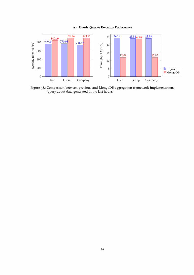
A.5. Hourly Queries Execution Performance

User Group Company0

200

400

600

800 759.46 770.05 741.47840.49

895.24 893.15A

vera

getim

e(u

s/op

)

User Group Company0

5

10

15

20

25 24.17 23.94 23.98

12.09

23.82

12.07

Thro

ughp

ut(o

ps/s

)

JavaMongoDB

Figure 38.: Comparison between previous and MongoDB aggregation framework implementations(query about data generated in the last hour).

86

A.6. Cache Performance

a.6 cache performance

Benchmark Score UnitsaverageFatigueByCompanyCurrentDay 278191.387 ± 2294.399 ops/saverageFatigueByCompanyCurrentMonth 274568.827 ± 2156.977 ops/saverageFatigueByCompanyCurrentWeek 575351.164 ± 5679.002 ops/saverageFatigueByCompanyLastDay 265446.917 ± 2487.687 ops/saverageFatigueByCompanyLastMonth 163570.197 ± 1501.222 ops/saverageFatigueByCompanyLastWeek 540436.522 ± 4600.465 ops/saverageFatigueByCompanyPerDay 704741.790 ± 7183.195 ops/saverageFatigueByCompanyPerMonth 712551.957 ± 6524.740 ops/saverageFatigueByCompanyPerWeek 512515.627 ± 4648.135 ops/saverageFatigueByGroupNameCurrentDay 277079.455 ± 2445.997 ops/saverageFatigueByGroupNameCurrentMonth 273284.238 ± 2271.772 ops/saverageFatigueByGroupNameCurrentWeek 585269.922 ± 4445.416 ops/saverageFatigueByGroupNameLastDay 268957.629 ± 2328.898 ops/saverageFatigueByGroupNameLastMonth 163267.525 ± 1711.443 ops/saverageFatigueByGroupNameLastWeek 542771.273 ± 4150.717 ops/saverageFatigueByGroupNamePerDay 706460.643 ± 5901.613 ops/saverageFatigueByGroupNamePerMonth 717570.553 ± 5572.612 ops/saverageFatigueByGroupNamePerWeek 511308.593 ± 4566.637 ops/saverageFatigueByUserCurrentDay 274687.748 ± 2480.478 ops/saverageFatigueByUserCurrentMonth 275349.263 ± 2344.364 ops/saverageFatigueByUserCurrentWeek 584568.297 ± 4814.899 ops/saverageFatigueByUserLastDay 266133.762 ± 2431.766 ops/saverageFatigueByUserLastMonth 163464.781 ± 1457.564 ops/saverageFatigueByUserLastWeek 544447.907 ± 4334.425 ops/saverageFatigueByUserPerDay 708642.074 ± 5533.543 ops/saverageFatigueByUserPerMonth 713253.697 ± 5509.457 ops/saverageFatigueByUserPerWeek 511827.517 ± 4689.561 ops/s

Table 25.: Throughput of the set of queries using the Cache system.

87

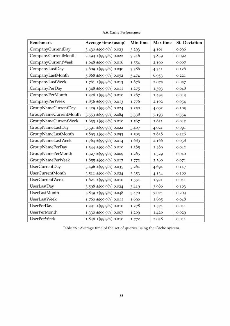
A.6. Cache Performance

Benchmark Average time (us/op) Min time Max time St. DeviationCompanyCurrentDay 3.430 ±(99.9%) 0.023 3.293 4.101 0.096

CompanyCurrentMonth 3.493 ±(99.9%) 0.022 3.346 3.859 0.092

CompanyCurrentWeek 1.648 ±(99.9%) 0.016 1.554 2.196 0.067

CompanyLastDay 3.609 ±(99.9%) 0.030 3.386 4.341 0.126

CompanyLastMonth 5.868 ±(99.9%) 0.052 5.474 6.953 0.221

CompanyLastWeek 1.761 ±(99.9%) 0.013 1.676 2.075 0.057

CompanyPerDay 1.348 ±(99.9%) 0.011 1.275 1.593 0.048

CompanyPerMonth 1.326 ±(99.9%) 0.010 1.267 1.493 0.043

CompanyPerWeek 1.856 ±(99.9%) 0.013 1.776 2.162 0.054

GroupNameCurrentDay 3.429 ±(99.9%) 0.024 3.250 4.092 0.103

GroupNameCurrentMonth 3.553 ±(99.9%) 0.084 3.338 7.193 0.354

GroupNameCurrentWeek 1.633 ±(99.9%) 0.010 1.567 1.821 0.042

GroupNameLastDay 3.591 ±(99.9%) 0.022 3.407 4.021 0.091

GroupNameLastMonth 5.893 ±(99.9%) 0.053 5.503 7.838 0.226

GroupNameLastWeek 1.764 ±(99.9%) 0.014 1.683 2.166 0.058

GroupNamePerDay 1.344 ±(99.9%) 0.010 1.285 1.489 0.042

GroupNamePerMonth 1.327 ±(99.9%) 0.009 1.265 1.529 0.040

GroupNamePerWeek 1.855 ±(99.9%) 0.017 1.772 2.360 0.071

UserCurrentDay 3.496 ±(99.9%) 0.035 3.264 4.694 0.147

UserCurrentMonth 3.511 ±(99.9%) 0.024 3.353 4.134 0.100

UserCurrentWeek 1.621 ±(99.9%) 0.010 1.554 1.921 0.041

UserLastDay 3.598 ±(99.9%) 0.024 3.419 3.986 0.103

UserLastMonth 5.849 ±(99.9%) 0.048 5.470 7.074 0.203

UserLastWeek 1.760 ±(99.9%) 0.011 1.690 1.895 0.048

UserPerDay 1.331 ±(99.9%) 0.010 1.278 1.574 0.041

UserPerMonth 1.330 ±(99.9%) 0.007 1.269 1.426 0.029

UserPerWeek 1.846 ±(99.9%) 0.010 1.772 2.038 0.041

Table 26.: Average time of the set of queries using the Cache system.

88