DAMS∗

Esther Duflo and Rohini Pande

Abstract

This paper studies the productivity and distributional effects of large irrigation dams in India.

Our instrumental variable estimates exploit the fact that river gradient affects a district’s suit-

ability for dams. In districts located downstream from a dam, agricultural production increases,

and vulnerability to rainfall shocks declines. In contrast, agricultural production shows an in-

significant increase in the district where the dam is located but its volatility increases. Rural

poverty declines in downstream districts but increases in the district where the dam is built,

suggesting that neither markets nor state institutions have alleviated the adverse distributional

impacts of dam construction.

∗Pande thanks NSF for financial support under grant SES-0417634. We thank, without implicating, the editorLawrence Katz, three anonymous referees, Marianne Bertrand, Michael Greenstone, Angus Deaton, Greg Fischer,Michael Kremer, Dominic Leggett, T.N. Srinivasan, Chris Udry, and, especially, Abhijit Banerjee and Chris Hansenfor comments and suggestions. We also thank James Fenske, Niki Klonaris, Callie Scott, and Hyungi Woo forexcellent research assistance, CIESIN at Columbia University for GIS help, and Abhijit Banerjee, Shawn Cole, SeemaJayachandran, Siddharth Sharma, and, especially, Petia Topalova for sharing their data.

1

I. Introduction

“If you are to suffer, you should suffer in the interest of the country.”

Indian Prime Minister Nehru, speaking to those displaced by Hirakud Dam, 1948.

Worldwide, over 45,000 large dams have been built, and nearly half the world’s rivers are ob-

structed by a large dam. The belief that large dams, by increasing irrigation and hydroelectricity

production, can cause development and reduce poverty has led developing countries and interna-

tional agencies such as the World Bank to undertake major investments in dam construction. By

the year 2000, dams generated 19 percent of the world’s electricity supply and irrigated over 30

percent of the 271 million hectares irrigated worldwide. However, these dams also displaced over 40

million people, altered cropping patterns, and significantly increased salination and waterlogging

of arable land [World Commission on Dams, 2000a]. The distribution of the costs and benefits of

large dams across population groups, and, in particular, the extent to which the rural poor have

benefited, are issues that remain widely debated.

Dams provide a particularly good opportunity to study the potential disjunction between the

distributional and productivity implications of a public policy. The technology of dam construction

implies that those who live downstream from a dam stand to benefit, while those in the vicinity

of and upstream from a dam stand to lose. From an econometric viewpoint, this implies that we

can isolate the impact of dams on the two populations, and from a policy perspective, this suggests

compensating losers is relatively easy. The inadequacy of compensation in such a comparatively

simple case would suggest that the distributional consequences of public policies are, perhaps,

harder to remedy than is typically assumed.

Proponents of large dam construction emphasize the role of large dams in reducing dependency

on rainfall and enabling irrigation, providing water and hydropower. In contrast, opponents argue

that while these benefits may be enjoyed by downstream populations, upstream populations benefit

only from the construction activity, and, potentially, from increased economic activity around the

reservoir. In the absence of compensation, they suffer potentially large losses; flooding reduces

agricultural and forest land, and increased salinity and waterlogging reduces the productivity of

land in the vicinity of the reservoir (McCully [2001] and Singh [2002]). Further, in order to fill the

2

dam reservoir, water use upstream is often restricted, especially in rain-scarce years. This increases

the vulnerability of upstream agricultural production to rainfall shocks (World Commission on

Dams [2000b] and Shiva [2002]).

What is striking in the policy debates surrounding dam construction is the absence of systematic

empirical evidence on how the average large dam affects welfare, especially of the rural poor. This

paper aims to provide such evidence. We focus on India, which, with over 4,000 large dams, is the

world’s third most prolific dam builder (after China and the United States). Large dam construction

is the predominant form of public investment in irrigation in India. Between 1950 and 1993, India

was the single largest beneficiary of World Bank lending for irrigation.1 An important justification

for such investment, both by the Indian government and the World Bank, is agricultural growth

and rural poverty alleviation (World Bank [2002], Dhawan [1993]).

A comparison of outcomes in regions with and without dams is unlikely to provide a causal

estimate of the impact of dams, since regions with relatively more dams are likely to differ along

other dimensions, such as potential agricultural productivity. To address this problem, we exploit

the fact, well documented in the dam engineering literature, that the gradient at which a river flows

affects the ease of dam construction. In particular, there is a non-monotonic relationship between

river gradient in an area and its suitability for dam construction. Low (but non-zero) river gradient

areas are most suitable for irrigation dams while very steep river gradient areas are suitable for

hydroelectric dams. Regions where the river gradient is either flat or somewhat steep are the least

likely to receive dams.

Our unit of analysis is the administrative unit below an Indian state, a district. We exploit

variation in dam construction induced by differences in river gradient across districts within Indian

states to obtain instrumental variable estimates. Our regressions control for differential state-

specific time effects, time-varying national effects of river gradient, and for other district geographic

features.

Our first set of results relate to agricultural outcomes. We use annual district-level agricultural

data and find that dam construction leads to a significant increase in irrigated area and agricultural

production in districts located downstream from the dam. Dams also provide insurance against

rainfall shocks in downstream districts. In contrast, dams have a noisy and typically insignificant

3

impact on agricultural production in the districts where they are built, and the vulnerability of

agricultural production to rainfall shocks significantly increases in these districts.

Our second set of results relate to rural poverty. Using district-level poverty data at five points

in time we find that dams significantly increase rural poverty in districts where they are located.

In contrast, poverty declines in districts downstream from the dam but,relative to the increase in

the dam’s district, this decline is small. Our poverty results are consistent with the findings of

agricultural production and volatility. It is worth noting, however, that with only five years of

poverty data, it is difficult to disentangle the poverty impact of dam construction from differential

time trends in poverty outcomes in districts suitable to dams construction relative to other districts

in the same states.2

Taken together, our results suggest a failure of state-level redistributive institutions. While we

cannot identify all the reasons for inadequate compensation of those who lose out, we are able

to show that the poverty impact of dam construction is accentuated in districts with a history

of relatively more extractive institutions (as captured by their historical land tenure systems, see

Banerjee and Iyer, [2005]). Our finding lends support to the view that institutions play an important

role in ensuring the distribution of productive gains between winners and losers.

In Section II, we describe the dam construction process in India, review the case study literature

on large dam construction in India, and use a simple production function framework to identify the

expected effects of dams. In Section III, we describe the empirical strategy. We provide empirical

results in Section IV and conclude in Section V.

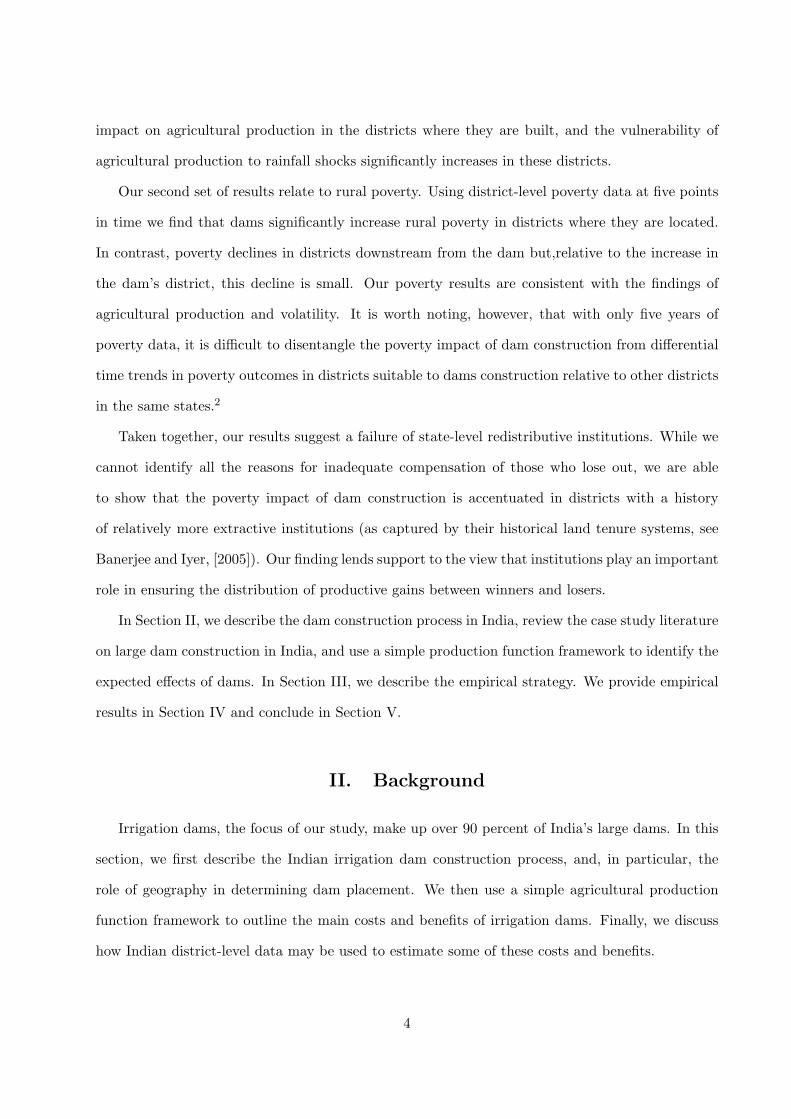
II. Background

Irrigation dams, the focus of our study, make up over 90 percent of India’s large dams. In this

section, we first describe the Indian irrigation dam construction process, and, in particular, the

role of geography in determining dam placement. We then use a simple agricultural production

function framework to outline the main costs and benefits of irrigation dams. Finally, we discuss

how Indian district-level data may be used to estimate some of these costs and benefits.

4

II.A. Dam Construction in India

Both the federal and state governments in India play an important role in dam construction.

The Indian Planning Commission (a federal body) sets each state’s five-year water storage and

irrigation targets. Given these targets and topological surveys of potential dam sites, the irrigation

departments of each State proposes dam projects. Next, a federal committee examines the economic

viability of these projects. The Planning Commission selects the final projects on the basis of

investment priorities and sectoral planning policies. Construction of a dam and the associated

canal network remain the State’s responsibility, though federal or international funding may be

available.

The typical Indian irrigation dam is an earth dam: water is impounded in a “reservoir” behind

an artificial wall built across a river valley. Artificial canals channel water from the reservoir to

downstream regions for irrigation. The area upstream from which water and silt flow into the

reservoir and the area submerged by the reservoir form the catchment area of the dam, while the

area downstream covered by the canal network is the command area.

The state government agency and farmers jointly manage the irrigation system associated with

a dam. The agency determines how much water to release to each branch outlet, and farmers served

by that outlet decide how to share it. Farmers working on land covered by the dam’s canal network

are eligible for dam irrigation. In contrast, to ensure that the reservoir is filled, the government

agency often restricts water withdrawal upstream from the reservoir (for instance, by cancelling

water pumping sites), especially in years of limited rainfall [Shiva, 2002].

The viability and cost of dam construction at a location depend crucially on its geography. The

ideal dam site is in a narrow river valley where the river flows at some gradient. Since current

satellite imagery resolution for India is too coarse for us to identify the width of a river valley, we

exploit the relevance of river gradient for dam construction.

The dam engineering literature provides multiple reasons as to why a river flowing at some

gradient is preferred for dam construction. The first reason relates to reservoir construction. Ac-

cording to the Handbook of Dam Engineering, [1977, p7], “to obtain economical storage capacity

5

a reservoir site should be wide in comparison to the dam site and should be on a stream having

a low or gentle gradient to obtain a long reservoir in proportion to the height of the dam.” The

second reason is that water flow from dams to the irrigated area is typically via gravity. Hence,

according to Cech [2003, p150-152] “Dams for irrigation projects are generally constructed at an

elevation high enough to deliver irrigation water to cropland entirely by gravity.” That said, the

river gradient should not be too steep because fast flowing water would erode the canal. US De-

partment of Agriculture, [1971, p 320-322] states that dam canals “should be designed to develop

velocities which are non-erosive for the soil materials through which the canal or lateral passes.”

Water velocity, and therefore the potential for erosion, increases with river gradient. As a result,

for irrigation dams, the recommended practice is to target dam sites where the river gradient in

the direction of irrigation is neither too steep nor completely flat.

In contrast, higher river gradient reduces the cost of producing hydroelectricity [Warnick, 1984].

To quote Cech [2003, p150-152], “Dams for hydroelectric power generation are located at a site

where the difference in elevations between the surface of the new reservoir and the outlet to the

downstream river is adequate to power electrical-generating turbines.”

To summarize, engineering considerations suggest that river gradient should have a non-monotonic

effect on the likelihood of dam construction. A river flowing through a flat area is less likely to see

dam construction while areas where the river flows at a moderate gradient should see more dam

construction. Finally, while areas with a steep gradient are less suited for irrigation, areas with a

very steep river gradient favor hydroelectric dam construction.

II.B. Benefits and Costs of Irrigation Dams

Between 1951 and 2000, food grain production in India nearly quadrupled, with two-thirds of

this increase coming from irrigated areas [Thakkar, 2000]. While dams account for 38 percent of

India’s irrigated area, estimates of what fraction of the increase in production can be attributed to

dams vary from 10 percent [World Commission on Dams, 2000b] to over 50 percent [Gopalakrishnan,

2000].

To clarify the potential role of dams in affecting agricultural production we describe a simple

6

agricultural production function framework, which is based on Evenson and McKinsey [1999].

We assume that agricultural output is a function of labor inputs L, land surface K, land quality

A, inputs such as fertilizer, seeds, and electricity I, climate r (rainfall and temperature), farmer’s

ability u, and a productivity shock ε. We denote the production function for land without access

to an irrigation system (via pump or canal) as

y = F1(L,K,A, I, r, u, ε),

and the production function for land with access to an irrigation system as

y = F2(L,K,A, I, r, u, ε).

Evenson and McKinsey [1999] estimate these production functions using Indian data. They find

that irrigation reduces the volatility of production by mitigating the effect of rainfall shocks and

temperature. Further, irrigation and agricultural inputs, such as fertilizer, electricity and seeds for

High Yielding Variety (HYV) crops are complements. These findings, and other studies such as

Singh [2002], suggest that irrigation enhances productivity by increasing multi-cropping and the

cultivation of more profitable water-intensive cash crops, especially sugarcane.

Assume that access to irrigation has a fixed cost. This is the cost of accessing ground water in

a region with no dams, and the cost of accessing canal irrigation in a dam’s command area. If a

farmer can obtain the optimal set of inputs, then she will invest in irrigation if its cost is below the

long-run difference between the value function with and without irrigation. Her decision process

follows a threshold rule: she switches if the productivity shock exceeds some threshold in a given

period.

Relative to other forms of water harvesting, such as ground water and small dykes, dams

reduce the fixed cost of accessing irrigation in the command area (Biswas and Tortajada [2001] and

Dhawan [1989]). Availability of dam irrigation will not affect the irrigation choices of farmers who

have paid the sunk cost of accessing ground water irrigation. However, those farmers who would

have invested in ground water irrigation in the future will instead opt for dam irrigation. Finally,

7

some of the farmers who would not have chosen ground water irrigation will invest in the cheaper

dam irrigation. Dams, therefore, increase irrigated area (though by less than the area actually

irrigated by the dams). Consequently, the demand for labor, fertilizer, and seeds will increase, and

the dependence of agricultural production on rainfall will decrease.

The impact of a dam is different in its catchment area. First, a significant fraction of land in the

catchment area is submerged during dam construction. For instance, the World Commission on

Dams [2000b] estimates that dam construction submerged 4.5 million hectares of Indian forest

land between 1980 and 2000. Land submergence is usually accompanied by large-scale population

displacement. Estimates of what fraction of the Indian population has been so displaced vary

between 16 and 40 million people. The World Commission on Dams [2000b] estimates that the

average Indian dam displaced 31,340 persons while a World Bank study in the mid-1990s estimated

a lower number of 13,000 people per dam [Cernea, 1996]. Case study evidence suggests that

historically disadvantaged scheduled tribe populations have borne the brunt of displacement.3

Second, water seepage from the canal and the reservoir increases waterlogging and soil salin-

ity and makes land less productive [Goldsmith and Hildyard, 1984]. The Indian Water Resources

Ministry estimated that roughly one-tenth of the area irrigated by dams suffered from either water-

logging or salinity/alkalinity by 1991 [World Commission on Dams, 2000b].4 While waterlogging

happens both around the canal and the reservoir (and therefore also affects the command area),

remote sensing studies suggest that these problems are more pronounced in the drainage area (for

instance, Khan and Sato, [2000] show that compared to the drainage network, irrigation canals are

relatively unaffected by this problem). This implies that irrigation in the catchment area is less

profitable, but fertilizer use may increase, since poorer soil requires more nutrients.

Finally, unaffected land in the catchment area upstream to the reservoir is unlikely to benefit

from dam irrigation, as lift irrigation is rarely practiced for dams [Thakkar, 2000]. In fact, govern-

ment agencies, which control the flow of water (through the opening of gates and sluices and the

control of water pumping sites), typically maximize water distribution through the canal network,

and to achieve maximum water storage in the reservoir, often restrict water use upstream from a

dam. Such restrictions are particularly prevalent in drought years when rainfall is insufficient to fill

the reservoir (see, for instance Shiva [2002] and TehriReport [1997]). As a result, the presence of

8

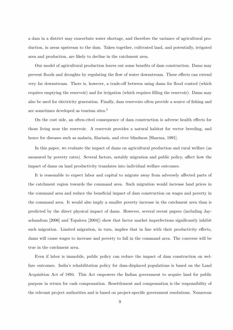
a dam in a district may exacerbate water shortage, and therefore the variance of agricultural pro-

duction, in areas upstream to the dam. Taken together, cultivated land, and potentially, irrigated

area and production, are likely to decline in the catchment area.

Our model of agricultural production leaves out some benefits of dam construction. Dams may

prevent floods and droughts by regulating the flow of water downstream. These effects can extend

very far downstream. There is, however, a trade-off between using dams for flood control (which

requires emptying the reservoir) and for irrigation (which requires filling the reservoir). Dams may

also be used for electricity generation. Finally, dam reservoirs often provide a source of fishing and

are sometimes developed as tourism sites.5

On the cost side, an often-cited consequence of dam construction is adverse health effects for

those living near the reservoir. A reservoir provides a natural habitat for vector breeding, and

hence for diseases such as malaria, filariasis, and river blindness [Sharma, 1991].

In this paper, we evaluate the impact of dams on agricultural production and rural welfare (as

measured by poverty rates). Several factors, notably migration and public policy, affect how the

impact of dams on land productivity translates into individual welfare outcomes.

It is reasonable to expect labor and capital to migrate away from adversely affected parts of

the catchment region towards the command area. Such migration would increase land prices in

the command area and reduce the beneficial impact of dam construction on wages and poverty in

the command area. It would also imply a smaller poverty increase in the catchment area than is

predicted by the direct physical impact of dams. However, several recent papers (including Jay-

achandran [2006] and Topalova [2004]) show that factor market imperfections significantly inhibit

such migration. Limited migration, in turn, implies that in line with their productivity effects,

dams will cause wages to increase and poverty to fall in the command area. The converse will be

true in the catchment area.

Even if labor is immobile, public policy can reduce the impact of dam construction on wel-

fare outcomes. India’s rehabilitation policy for dam-displaced populations is based on the Land

Acquisition Act of 1894. This Act empowers the Indian government to acquire land for public

purpose in return for cash compensation. Resettlement and compensation is the responsibility of

the relevant project authorities and is based on project-specific government resolutions. Numerous

9

studies suggest compensation rights of the landless, and those without formal land titles, are typi-

cally not recognized [Thukral, 1992]. Further, compensation is usually insufficient for the displaced

to replace lost land by its equivalent in quality and extent elsewhere [Dreze, Samson, and Singh,

1997].

A related policy intervention would be to charge the downstream population for water usage.

However, water charges in India remain so low that they often do not even cover the operation and

maintenance costs of the canal system [Jones, 1995].6 In fact, Prasad and Rao [1991] show that

tax collection costs often exceed the amount collected. The inability, or unwillingness, to charge an

appropriate fee for water has three consequences: farmers in the command area have been encour-

aged to switch to water intensive crops, thereby, according to some, seriously limiting the gains

in water availability; the canal systems are poorly maintained, which reduces their effectiveness

[Jones, 1995]; and redistribution of any benefits is limited.

II.C. Districts as the Unit of Analysis

We will estimate the effect of dams on economic outcomes at the district level, which is the

lowest level of disaggregation for which household consumption and agricultural production data

is available.

A district is the administrative unit immediately under the Indian state (somewhat analogous

to a county in the United States) and forms the natural unit for the planning and implementation

of state policies. In 1991, India had 466 districts, with a district, on average, having a population

of 1.5 million and an area of 8,000 square kilometers.

The absence of data on the geographic extent of the catchment and command areas of large

Indian dams prevents us from identifying the fraction of district area covered by the catchment

and command areas of each dam. Available catchment and command area maps suggest that the

district in which the dam is physically located usually contains most or all of its catchment area,

even for large dams.7

Water distribution in the command area of a dam is usually via gravity through artificially

constructed canals. The command area lies downstream from the reservoir, with the canal network

10

extending in the downstream direction along the main canal and often covering parts of multiple

districts.8

The estimated effect of a dams in the district where it is built combines the effects in catchment,

command, and unaffected areas, and is a priori ambiguous. The effect of a dam on agricultural

production in the neighboring downstream district should be unambiguously positive (since it only

has part of the command area), but will underestimate the command area effect (both because

some (or all) of the downstream district will not be in the command area, and because part of the

command area will not be in that district). But it is reasonable to expect that the dam’s own district

and the neighboring downstream districts will be the most affected by the dams. In Table IV, we

examine the effect of dams in all neighboring districts and find that, on average, dams only affect

production and rural welfare in the district where they are built and in neighboring downstream

districts. Our estimates are not quantitative estimates of the impact of the dam in its command and

catchment areas, but rather its impact on the most relevant corresponding administrative units.

Finally, aside from the fact that consistent data is available at the district level, a district-level

analysis presents one important advantage: districts are relevant markets and social units within

which people might relocate (for example, because they were displaced or their land became less

productive), but migration across district lines in response to shocks is rare.

III. Empirical Strategy

Our analysis exploits detailed Indian district panel data on district geography, dam placement,

and poverty and agricultural outcomes. We have annual agricultural production data for 271

districts for 1971-1999, and poverty data for 374 districts for five years: 1973, 1983, 1987, 1993,

and 1999. Table I provides descriptive statistics and the Data Appendix describes the data sources

and variable construction.

Between 1971 and 1999 the number of large dams in India quadrupled from 882 to 3,364, and

the average number of dams in a district increased from 2.39 to 8.66 (46 percent of the districts

had no dams in 1999). There was significant regional variation in dam construction. Figures I

and II, which depict district-wise dam construction in 1970 and 1999 respectively, show that dam

11

construction was concentrated in western India, with relatively little dam construction in North

and Northeastern India. Figure III graphs overall dam construction in India. Dam construction

was rapid between the mid-1970s and late 1980s, but slowed down considerably in the 1990s.

OLS regression estimates of how the number of dams in a state affect agricultural, or welfare,

outcomes are unlikely to be consistent. Richer and fast growing states can build relatively more

dams. States that anticipate larger increases in agricultural productivity are also likely to make

more of these investments, implying a spurious positive relationship between poverty reduction and

agricultural growh and dam building. Indeed, Merrouche [2004] finds larger poverty reductions for

states that built more dams, but these findings cannot be given a causal interpretation.

Our identification strategy, therefore, relies on within-state differences in dam construction,

specifically differences across districts in a state. We can, therefore, examine spillover effects from

dams in neighboring districts, but not state-wide economic effects of dam construction, such as their

effect on prices determined at the state level. We discuss the possible direction of such state-wide

effects as we interpret our results.

Consider the following regression:

(1) yist = β1 + β2Dist + β3DUist + β4Zit + β5Z

Uit + νi + µst + ωist

where Dist denotes the number of dams in the district and DUist the number of dams located

upstream from district i. νi is a district fixed effect, µst is a state-year interaction effect and ωist

a district-year specific error term. Zit and ZUit are a set of time varying control variables for the

district and for upstream districts (the list of relevant control variables is discussed below).

District fixed effects allow us to control for time-invariant characteristics that affect the likeli-

hood of dam construction in the district and state-year interactions for annual shocks, which are

common across districts in a state. We only exploit cross-district variation in dam construction in

a state for identification.

Within states, the residuals from regressions using annual agricultural data are strongly auto-

correlated. In this setting, estimating generalized least squares, rather than OLS, regressions can

potentially increase efficiency. We compute feasible GLS estimates (FGLS) using the method pro-

12

posed by Hansen [2006]. First, we obtain the time series process for the regression residual (after

correcting for biases due to the small sample and inclusion of fixed effects). An AR(2) process best

reflects the data, except for wages.9 We use these parameters to construct the FGLS weighting

matrix. Misspecification in the time series process can cause the conventional FGLS standard errors

to over-reject the null hypothesis [Bertrand, Duflo, and Mullainathan, 2004]. Therefore, we report

standard errors, which are robust to arbitrary covariance of the FGLS residual within the state

(Wooldridge [2003] and Hansen [2006]).10

For OLS and GLS estimates to be consistent requires that the annual variation in dam construc-

tion across districts within a state be uncorrelated with other district-specific shocks. However,

this assumption may be violated if, for instance, agriculturally more productive districts witness

relatively greater dam construction. To address this problem, we develop an instrumental variable

strategy based on the geography of dam construction.

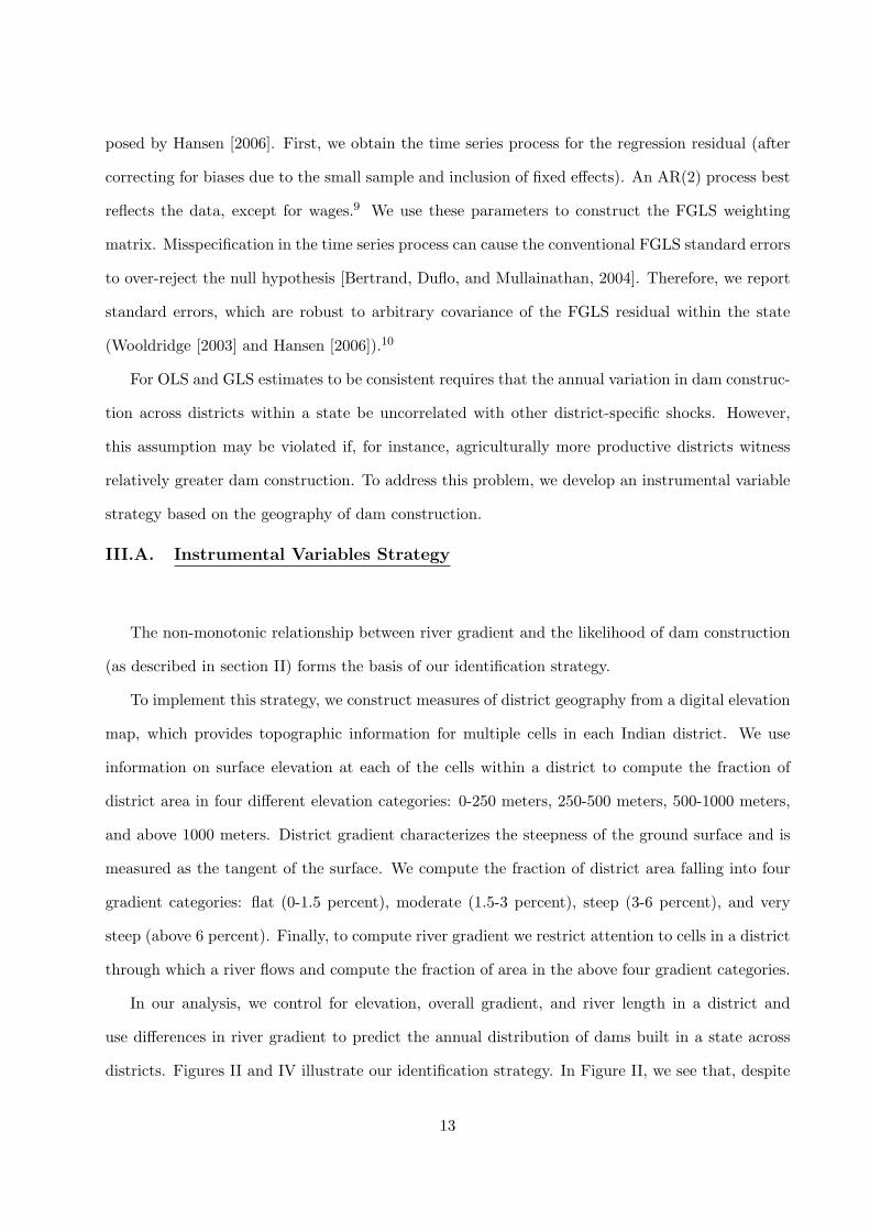
III.A. Instrumental Variables Strategy

The non-monotonic relationship between river gradient and the likelihood of dam construction

(as described in section II) forms the basis of our identification strategy.

To implement this strategy, we construct measures of district geography from a digital elevation

map, which provides topographic information for multiple cells in each Indian district. We use

information on surface elevation at each of the cells within a district to compute the fraction of

district area in four different elevation categories: 0-250 meters, 250-500 meters, 500-1000 meters,

and above 1000 meters. District gradient characterizes the steepness of the ground surface and is

measured as the tangent of the surface. We compute the fraction of district area falling into four

gradient categories: flat (0-1.5 percent), moderate (1.5-3 percent), steep (3-6 percent), and very

steep (above 6 percent). Finally, to compute river gradient we restrict attention to cells in a district

through which a river flows and compute the fraction of area in the above four gradient categories.

In our analysis, we control for elevation, overall gradient, and river length in a district and

use differences in river gradient to predict the annual distribution of dams built in a state across

districts. Figures II and IV illustrate our identification strategy. In Figure II, we see that, despite

13

the presence of one of the world’s largest river basins, the Indo-Gangetic basin, almost no dam

construction has occurred in North India. Figure IV depicts the average river gradient – central

North India has very flat rivers, while most of Western India, which has seen the maximum dam

construction, has rivers with moderate gradient.

In column (1) of Table II, we formally examine the relationship between the number of dams

built in a district by 1999 and district river gradient. Our regressions include state fixed effects,

district elevation, river length, and district gradient as controls. The omitted river gradient category

is the proportion of river in the flat gradient category (0-1.5 percent). Our results confirm the

importance of engineering considerations: a gentle river gradient (1.5-3 percent) increases the

number of dams, while a steep gradient reduces it. However, a very steep river gradient (more than

6 percent) increases dam construction. The last effect is attributable to some multipurpose dams

in our sample that provide both irrigation and hydroelectricity.11

Our panel regressions build on these findings. To predict the number of dams in a district, we

exploit three sources of variation in dam construction: differences in dam construction across years

in India, differences in the contribution of each state to this increase, and finally differences across

districts within a state that are driven by the geographic suitability of districts.

We estimate panel regressions of the form

(2) Dist = α1 +4∑

k=2

α2k(RGrki ∗Dst) + α3(Mi ∗Dst) +4∑

k=2

α4k(RGrki ∗ lt) + νi + µst + ωist

where Dist is the number of dams in district i of state s at time t. νi, the district fixed effect,

accounts for time-invariant district characteristics, which may affect dam building, and µst, the set

of state-year interactions, accounts for the impact of state-level macro shocks.

RGrki denotes the river gradient variables. These enter the regression interacted with predicted

dam incidence in the state, Dst. This is constructed by multiplying total dam construction in India

with the fraction of total dams in the state in 1970. Use of predicted, rather than actual, dam

incidence ensures that the measure is exogenous with respect to the number of dams in the district.12

The interaction of the RGrki variables with year dummies (lt) accounts for national time-varying

effects of river gradient on the outcomes of interest. Mi, the vector of district-specific time-invariant

14

control variables, includes district elevation and overall gradient measures, river length, and district

area.

Column (2) of Table II provides coefficient estimates for the poverty sample (five years of data)

and column (3) for the agricultural production sample (twenty nine years of data). The results are

similar to the cross-sectional regression in column (1), except that the interaction of the proportion

of district in the very steep gradient category and the predicted number of dams is significant. The

F-statistics demonstrate that the instruments have sufficient power.

Let Zist denote the vector of right-hand side variables in equation (2), except for the interactions

RGrki ∗Dst. Similarly, define ZUist as the vector, which includes the same control variables for the

upstream district.13 We estimate:

(3) yist = δ1 + δ2Dist + δ3DUist + Zistδ4 + ZUistδ5 + νi + µst + ωist.

To generate instruments for Dist and DUist, we use parameters from equation (2) to predict the

number of dams per district Dist. For upstream districts, the predicted number of dams, DUist, is

the sum of predicted values from equation (2) for all upstream districts (it equals zero if the district

has no upstream district). We estimate equation (3) using Dist, DUist, Zist, and ZUist as instruments.

The first-stage equation is:

(4) ∆ist = φ1 + φ2Dist + φ3DUist + Zistφ4 + ZUistφ5 + νi + µst + ωist

where ∆ist represents Dist or DUist.

Our procedure uses available information efficiently: by using all districts to predict the rela-

tionship between district geographic features and the number of dams (rather than just those that

are upstream), we avoid averaging these features when there are several upstream districts.14

In the regression using annual data, we estimate equation (3) by feasible optimal IV (the

equivalent of FGLS for IV). As with FGLS, we report standard errors that are robust to arbitrary

covariance of the residual within a state.15

Our instrumental variable strategy exploits variation in the interaction of the river gradient

15

variable in the district (or in the upstream district) with predicted dam construction in the state

(that is, the interaction of the 1970 share of dams in a state with dam construction in India). The

inclusion of the interaction of river gradient with year dummies controls for any differential trends

across regions with different river gradients. In particular, we control for the fact that the ease of

non-dam irrigation in regions with different river gradients may vary.16

The identifying assumption underlying our analysis is that absent dam construction, the evo-

lution of economic outcomes across districts located in the same state but with different river

gradients would not have systematically differed across states with more dams in 1970 and states

with fewer dams in 1970. In 1970, Gujarat, Madhya Pradesh, and Maharashtra were the three

States with the most dams. Gujarat and Maharashtra are among India’s richer states, though their

agricultural income growth is not the highest in our sample. Still, one may worry that our instru-

ment is picking up non-dam-related differences in growth patterns across districts with different

river gradient characteristics in richer and poorer states.

To address this concern, we report additional specifications. First, Figure III suggests that, at

least for outcomes for which we have annual data, the time pattern of evolution of outcomes due

to dam construction can potentially be distinguished from a linear trend that differs across regions

with different river gradient. We, therefore, examine whether our results are robust to including as

an additional control the interactions of a linear trend with the share of dams built by the state in

1970 and the river gradient variables (and the similar interactions with the upstream river gradient

variables). Second, we check that our results are robust to including as additional controls the

initial tribal population share and initial poverty in the district, each interacted with the predicted

dam share in the state Dst (and the corresponding interactions with upstream tribal share and

poverty). This addresses the concern that regions favorable to dams may have also differed in

terms of their initial poverty or tribal population shares, and that these initial conditions, not dam

construction, determined subsequent agricultural and poverty changes.

In reality, dams vary significantly, both in their physical characteristics (this includes dam height

and canal network) and in their location (for instance, the productivity of surrounding agricultural

land). Our IV estimates capture the “local average treatment effect” of dams, or their effect in

districts where dams were built because the districts had favorable river gradients and which would,

16

otherwise, not have received dams. Likewise, our upstream dam variable captures the effect of dams

that were located upstream for a district because the river gradient in the upstream district was

favorable. In other words, what we do not capture is the effect of dams placed in specific districts

for, say, political reasons. This may imply that our estimates are close to a “best case scenario,”

since we are measuring the economic impact of technologically appropriate dams. We recognize

that this may differ from the impact of the “average” dam. While explicitly examining the impact

of, say, different-sized dams could shed some light on this, our instruments do not have sufficient

power for this. 17

IV. Results

IV.A. Agriculture

We start by examining how large dams have affected irrigated and cultivated area and agricul-

tural production, both in the district where they are constructed and downstream. We have annual

data for 271 districts for the years 1971-1999. Panel A of Table III provides FGLS estimates (equa-

tion (1)), and Panel B Feasible Optimal IV estimates (equation (3)). The “own district” coefficient

captures the impact of dams built in that district while the “upstream” coefficient captures the

impact of dams built in neighboring upstream districts (and we often refer to this as the down-

stream effect of dams). In the last row, we report the F-statistic for the first-stage regression for

the “own district” dams (using the variable “dams predicted in own district”). The instruments

appear sufficiently strong to avoid bias caused by weak instruments.18

A first observation, and one to which we return below, is that the standard errors on the

estimated “own district” coefficient always exceed those of the “dams upstream” coefficient.

In columns (1)-(4) we report level and log estimates for irrigated and cultivated area.19 The

IV estimates indicate a significant increase in gross irrigated area in downstream districts – an

additional dam increases irrigated area in the downstream district by roughly 0.33 percent or 497

hectares (this estimate is statistically indistinguishable from the FGLS estimate). The effect on

irrigation in own district is also positive. The point estimate is similar to the downstream effect in

17

the FGLS specification and larger in the IV specification. However, the associated standard errors

are also very large (below we suggest possible explanations).

In columns (6) and (7) we consider the production and yield of the six major crops in districts

(in logs). Both the FGLS and Optimal IV estimates suggest that dam construction significantly

increases agricultural production (0.34 percent) and yield (0.19 percent) in the downstream districts.

In contrast, own district estimates are smaller and insignificant.

Case study evidence (and our model) suggests that dam irrigation causes farmers to substitute

towards water-intensive crops. In columns (8) and (9) of Table III, we see that dams had an insignif-

icant impact on non-water-intensive crop production, but significantly increased the production of

water-intensive crops in downstream districts. We find similar sized, but much noisier estimates,

for water-intensive crop production in own district.20

Table III provides a very consistent pattern for how dams affect agricultural production in

downstream districts: they significantly increase irrigated area and agricultural production, espe-

cially of water-intensive crops. In contrast, the effect on production in own district is typically

insignificant.

To the best of our knowledge, there are no other systematic estimates of the impact of dams

on agricultural outcomes to which we can compare our estimates. However, we can provide two

checks on whether the magnitude of estimated effects are plausible.

First, we can use direct estimates of the physical area irrigated by dams. Dam irrigation, in

part, substitutes for alternative forms of irrigation. This suggests our estimates of the additional

area irrigated due to dams should be lower than the actual area irrigated by dams. Our point

estimates suggest that dams increased area irrigated in each downstream district by 497 hectares,

and 2,321 hectares in own district. There are, on average, 1.75 districts downstream from a dam.

This suggests that an additional 3,191 hectares are irrigated by a dam. This number can be

compared to estimates of the average area irrigated by a dam. The Indian Planning Commission

estimated that a dam irrigated 8,759 hectares in 1985. This estimate suggests that 36 percent of

the area irrigated by dams would not have been irrigated otherwise.

Second, if we assume that the sole effect of dams on production downstream is through irri-

gation, then our instrument for having a dam upstream is also an instrument for area irrigated.21

18

This procedure gives us an elasticity of production with respect to dam-induced irrigation of 0.61

(standard error of 0.21, estimate not reported to save space). Relative to existing estimates, this

is a plausible elasticity, though in the lower range.22

Robustness In Tables IV and V, we check that our production results are robust to alternative

specifications.23

In panel A of Table IV, we show that the production effects of the average dam do not extend to

neighboring districts that are not downstream. This suggests that our focus on the impact of dams

on the districts where they are located and downstream districts is reasonable. In Panel B, we

examine whether changes in agricultural production precede dam construction. We include dams

in own district and upstream that are currently under construction and will be completed in the

next five years as additional regressors. We find no evidence that agricultural production increases

in the five years prior to dam completion.

In Table V, we first include an array of additional controls. In column (1), we control for

the interaction of initial poverty in the district (and in the district upstream) with predicted dam

construction in the state, and in column (2), we similarly control for initial tribal population.

Our production estimates are unaltered. In column (3), we show that our results are robust to

controlling for a linear time trend interacted with the state’s share of total dams in 1970. Finally,

in column (4), we show that our results are also robust to normalizing the number of dams by

district area.

Variance of Production Why are the estimated effects of dams so much noisier in the dam’s

own district than in the downstream district? One reason is that the own district effect combines

the (presumably negative) catchment area effect with a (presumably positive) effect in the part

of the command area that falls within the district. The combined effect is likely to vary across

districts, depending, for instance, on dam size and its location within the district. Such variability,

in turn, would imply noisier estimates of the average effect.

Another possible reason (which does not exclude the above) is that dams affect the variance of

agricultural production differentially across own and downstream districts. An important cause of

annual variations in crop production across Indian districts is rainfall shocks. Dams are likely to

19

reduce the sensitivity to rainfall shocks downstream, but to increase it in the upstream areas, due

to restriction on water usage.

In Table VI, we examine whether dams mediate or amplify the effect of a rain shock on agri-

cultural production. We measure rain shock as the fractional deviation of annual rainfall from the

district’s historical average.24 In column (1), we see that, controlling for dam presence, a posi-

tive rain shock enhances agricultural production. Column (2) shows that having a dam upstream

reduces the adverse effect of a negative rain shock: the coefficients on the upstream dam’s rain

shock interaction variable and the rain shock variable have opposite signs, and both coefficients are

significant. In contrast, dams amplify the effect of a rain shock in own district. The coefficients on

own district dam’s rain shock interaction variable and the rain shock variable have the same sign,

and the interaction with dams is significant.

Our finding suggests that dams increase the variance of agricultural production in own dis-

trict, without significantly increasing the mean production in the average district. If risk aversion

decreases with income, then this increase is likely to be particularly harmful to the poor.

Other Inputs Consistent with the predictions of a simple agricultural production function, we

find that dams increase the production of water-intensive crops in downstream areas; two of these

crops (rice and wheat) saw increased use of high yielding variety seeds. Column (5) in Table III

also shows that dams led to an insignificant increase in fertilizer use.

The agricultural production function also suggests that dam irrigation should reduce the use of

alternative forms of water infrastructure and increase electricity and fertilizer use (because canal

irrigation requires electricity). In Table VII, we examine the impact on other inputs using decen-

nial census data.25 Columns (1) and (2) provide some, albeit weak, evidence that non-dam-related

water infrastructure decreased (the number of canals shows an insignificant increase), and electrifi-

cation increased in downstream districts. Other measures of infrastructure are unchanged by dam

construction (see column (3)) and suggest no crowding in (or out) of other government inputs.

20

IV.B. Rural Welfare

Using our estimates to undertake a cost-benefit analysis of dam construction requires additional

assumptions about the construction and operation costs of dams. We also need to make assumptions

about unmeasured benefits and costs, such as the value of insurance downstream, possible effects

in other neighboring districts that are too small to detect (although, on average, we do not observe

any such effects), and agents’ optimizing behavior.

A different approach to assessing the overall impact of dams, and one we take, is to examine

how large dams have affected the welfare of the rural poor. Agriculture is the main occupation of a

majority of the rural poor, and India’s five-year plan documents (which identify, on a five-year basis,

the government’s policy priorities), show that an explicit aim of public investment in irrigation is

to increase agricultural productivity, reduce instability in crop production, and enhance the welfare

of the rural poor. For instance, the opening chapter of India’s fifth five-year plan document begins,

‘The objectives in view are removal of poverty and achievement of self-reliance’.

We begin by examining the implications of dam construction for district demographics. This

is an interesting question in and of itself, and is also relevant for interpreting our poverty results

(since our dataset is a panel of districts, rather than of individuals, the estimated effect of dam

construction on poverty would be biased if dam construction induces either the relatively rich or

relatively poor individuals to migrate across district boundaries). Columns (4) and (5) of Table VII

report insignificant effects of dam construction on district census rural population outcomes, both

overall population and in-migrants. A potential explanation is that imperfect credit and insurance

markets inhibit labor mobility by the poor in response to regional economic shocks. Our findings

are in line with anecdotal and case study evidence that suggests that displaced populations prefer to

remain near their original habitats [Thukral, 1992]. Other studies also find very limited migration

in response to relatively large district-level economic shocks.26 These findings also imply that it

is reasonable to use a district-level panel on poverty outcomes to examine how dam construction

affects rural welfare. That said, we compute bounds on how migration may have affected the

estimated impact of dams on poverty [Manski, 1990].

Our welfare results are in Table VIII; Panel A provides OLS estimates and Panel B 2SLS

21

estimates.27 Column (1) shows that dams lead to an insignificant decline in mean per capita

expenditure in the district where they are located and a marginally significant increase in per

capita expenditure in downstream districts. In column (2), we examine the most basic rural poverty

indicator: the head count ratio. This measures the fraction of rural households with a consumption

level below the official poverty line. Each dam is associated with a significant poverty increase of

0.77 percent in its own district. In contrast, poverty decreases in downstream districts. Columns

(3) and (4) bound our poverty results by making alternative assumptions about migration (we use

the Table VII point estimates for in-migrants even though they are insignificant). The poverty

results remain robust.28

Since there are, on average, 1.75 districts downstream of each dam, the poverty reduction in

downstream districts is insufficient to compensate for the poverty increase in the dam’s own district.

Another way of computing the overall poverty effect is to start with the observation that between

1973 and 1999 the average district had five dams built in own district and ten dams upstream.

Our point estimate implies that this led to a 2.35 percent increase in the head count ratio (5*0.77-

10*0.15). Over this time period, the head count ratio reduced by 23 percent, suggesting that

poverty reduction in the average Indian district may have suffered as much as a 10 percent setback

due to dam construction. An important caveat is that we have not accounted for either state-wide,

or small, effects that diffused over a large area.

Column (5) examines an alternative measure of rural poverty, the poverty gap. This measures

the depth of poverty – specifically, how much income is needed to bring the poor to a consumption

level equal to the poverty line. In line with our earlier results, we find that dams significantly

increase the poverty gap in their own district, while reducing it downstream.

Column (6) examines within-district inequality as measured by the Gini coefficient. Dam con-

struction did not significantly affect inequality, either in its own district or downstream districts.

This suggests the main unequalizing effect of dams was across, not within, districts. In column (7),

we find that dams lead to significant increases in male agricultural wage growth in downstream

districts. This is consistent with our poverty findings – male agricultural wages are considered a

important driver of poverty.

Finally, in column (8), we examine whether dams affect health outcomes, as measured by annual

22

malaria incidence between 1976 and 1995. We find no evidence that dams increased the district-

level prevalence of waterborne diseases, here malaria. This suggests that negative health effects did

not drive the observed increase in poverty.

Robustness In panel A, Table IV, we show that, similar to agricultural production, the poverty

effects of dam construction do not extend to neighboring districts that are not downstream. In

panel B, we include dams in own district and upstream that will be completed in the next five

years as additional regressors. If dam construction activity itself lowered poverty, then comparing

poverty outcomes before and after dam construction may lead us to overestimate their negative

effect. Dam construction activity does not reduce poverty, in fact, poverty increases while dams are

under construction. This is consistent with the fact that population displacement in the vicinity of

the reservoir occurs during the construction period.

In columns (5)-(7) of Table V, we introduce additional controls to check for differential trends

across districts with varying initial conditions. Our poverty results are robust to controlling for the

separate interaction of the predicted number of dams in the state with initial poverty and tribal

population share (columns (5) and (6)).

In column (7) we include the triple interaction of a linear time trend, the initial dam incidence

in the state (as a fraction of total dam construction in 1970) and the river gradient in the district.

As with agricultural production, this specification is intended to control for the possibility that

the trend in economic outcomes in a district which is more suitable for dam construction differed

from that in other districts in the same state, and that this also differed in states that built more

dams. We find that while the results for the downstream district hardly change, the standard

error of the own district estimates more than doubles (to 0.765), and the point estimates drops (to

0.25). The confidence interval includes both the previous estimate and zero.29 A likely reason for

this is the limited time series for poverty data; with only five years of data, the time pattern of

dam construction across India is difficult to disentangle from a linear trend, and there is very little

identifying variation left. That said, this specification provides a relevant caveat to the robustness

of the own-district poverty results.

23

Poverty and Rainfall In addition to displacement and the loss of productivity of the land

around the reservoir, the increased variance of production in the district where a dam is built may

interact with low levels of migration and closed markets to amplify negative shocks and increase

poverty (Jayachandran 2006). Given limited access to insurance against risk in rural India and

limited insurance options (Morduch (1995), Rosenzweig and Binswanger (1993) and Rosenzweig

and Wolpin (1993)), this is a potentially important channel through which dam construction can

increase poverty. In columns (3)-(6) of Table VI, we examine whether dams amplify or reduce the

poverty effect of rainfall shocks. In columns (3) and (5) we observe that, controlling for dams,

positive rainfall shocks reduce both the head count ratio and the poverty gap. In columns (4)

and (6), we examine whether dams alter the impact of rainfall shocks on poverty outcomes. Dams

weakly reduce the impact of rainfall shocks on poverty in downstream districts, but significantly

amplify it in the district where the dam is constructed. This is particularly true for the poverty

gap, which accounts for depth of poverty; our finding is particularly worrisome as it suggests dams

have worsened outcomes for households whose welfare was the lowest to begin with.

Institutions, Politics, and Dams The inability or unwillingness of those who benefit from

dams to compensate groups of losers, or of the state to require them to do so when both groups

are clearly identifiable ex-ante, suggests poorly functioning institutions of redistribution.

The absence of a statutory rehabilitation law, or even a national policy for rehabilitation, implies

that state governments and project authorities face no legal imperative to undertake rehabilitation

planning. World Commission on Dams (2000b) describes the rehabilitation policies of Indian

states as “knee-jerk reactions to the manifestations of disaffection of populations on land which is

acquired for public purposes.” Such arbitrariness suggests that actual compensation may depend

on the ability of affected population groups to organize themselves and lobby government and

project authorities. To explore this possibility, we examine whether the welfare consequences

of dam construction vary with the presence of historically disadvantaged population groups and

institutional quality.

Tribal populations in India face significant socioeconomic disadvantage, and case study evi-

dence suggests that these groups have faced significant dam-induced population displacement. We,

24

therefore, use the 1971 tribal population share in a district as our measure of the socioeconomic

disadvantage faced by the district population.

To measure institutional quality, we use district-level data on historic land tenure arrangements.

During the colonial period, the British instituted different land revenue collection systems across

districts. In some districts, an intermediary (usually a landlord) was given property rights for

land and tax collection responsibilities. In other districts, farmers were individually or collectively

responsible for tax collection. In “landlord” districts, a class of landed gentry, who had conflictual

relationships with the peasants, emerged. Banerjee and Iyer (2005) show that the ability of the

population to organize themselves and obtain public goods exhibited marked differences across

regions with different historical land tenure legacies. In landlord districts, class relations remain

tense, rendering collective action more difficult. These districts continue to have lower public

good provision, agricultural productivity, and higher infant mortality.30 If the population groups

affected by dam construction are better able to organize themselves and obtain compensation in

non-landlord districts, then the poverty impact of dam construction should be muted in these

districts. To examine this, we construct and use a non-landlord dummy that equals one: the tax

revenue system of the district was not landlord-based prior to Independence.

In Table IX, we report regressions, which include the separate interactions of the dam’s variable

with the 1971 district tribal population share and the non-landlord district dummy as additional re-

gressors (our instrument set is as before, plus the interaction with the tribal and landlord variables).

Our sample is restricted to districts that were under direct British rule.

Column (1) shows that the impact of dams on agricultural production did not differ across

landlord and non-landlord districts. Nor did it vary with the tribal population share. This suggests

that technological, rather than institutional, factors determine the productivity effect of a dam.

Columns (2) and (3) consider poverty outcomes. The poverty impact of dams is independent of

the tribal population share of the district. However, historic land tenure arrangements significantly

affect the poverty implications of dam construction. The effect of dams on poverty in own district

is halved in non-landlord districts, and we cannot reject the hypothesis that dams do not increase

poverty in non-landlord districts. We conjecture that in non-landlord districts, the population is

more effective in organizing itself to demand compensation from the state. It is also possible that

25

the absence of the landed gentry gives the displaced more political power in non-landlord districts.31

These findings point to the relevance of the institutional framework within which public policies,

such as dam construction, are executed and suggests that “weak institutions” or social conflict

may help explain the claim that the distributional consequences of dam construction have been

particularly adverse in developing countries.

V. Conclusion

In 2000, public spending on infrastructure in developing countries averaged 9 percent of govern-

ment spending, or 1.4 percent of GDP. Despite the magnitude of such spending, and a widespread

belief that infrastructure is integral to development, evidence on how investment in physical infras-

tructure affects productivity and individual wellbeing remains limited [World Bank, 1994].

In this paper, we have examined these questions in the context of large dam construction in

India. We have argued that any credible evaluation of large dams must address the fact that

dam placement is likely to be affected by regional wealth and the expected returns from dam con-

struction in a region. This problem of endogenous placement arises in the evaluation of any large

infrastructure project [Gramlich, 1994]. While cross-country evidence finds that productive gov-

ernment spending enhances growth, most studies are unable to convincingly control for unobserved

heterogeneity (see, for instance, Canning, Fay, and Perotti [1994] and Esfahani and Ramirez [2003]].

Exploiting geographic suitability for infrastructure allows us to address this concern and estimate

returns to infrastructure investment.

Large dams in India have benefited downstream populations. In contrast, those living in the

vicinity of the dam fail to enjoy any agricultural productivity gains and suffer from increased

volatility of agricultural production. Our poverty results also suggest a worsening of living standards

in the district where the dam is built; though limited data availability for the poverty outcomes

limits our ability to wholly disentangle the poverty impact of dam construction from district-specific

time trends in poverty which are correlated with geographic suitability for dams.32

These findings have important policy implications. In Spring 2005, the World Bank announced

270 million dollars in grants and guarantees for the Nam Theun 2 dam in Laos. The New York

26

Times (June 5, 2005) quotes a senior World Bank official, who justifies the return to dam lending

as driven by the need to support infrastructure development in a “practical” way since, “You’re

never ever going to do one of these in which every single person is going to say, ‘This is good for

me’”[Fountain, 2005]. Implicit in this statement is the belief that projects with an average positive

return should be undertaken, as it will be possible to compensate the losers. We, however, find

an unequal distribution of the costs and benefits associated with large dam construction in India

and provide suggestive evidence that an important reason for this is institutional quality. In areas

where the institutional structure favors the politically and economically advantaged, large dam

construction is associated with a greater increase in poverty. Whether institutional quality could

also explain the extent of dam construction across India is left for future research.

27

VI. Data Appendix

DamsData on dams is from the World Registry of Large Dams, maintained by the International Commis-sion on Large Dams (ICOLD). A large dam is defined as a dam ’having a height of 15 meters fromthe foundation, or, if the height is between 5 to 15 meters, having a reservoir capacity of more than3 million cubic meters. The registry lists all large dams in India, completed or under construction,together with the nearest city to the dam and date of completion. We use city information toassign dams to districts in the year of completion. The nine states in our sample without dams areArunachal Pradesh, Mizoram, Nagaland, Punjab, Sikkim, Dadra and Nagar Haveli, Daman andDiu, Delhi, and Pondicherry. Punjab and Delhi have dams in neighboring upstream states.GeographyDistrict area, river kilometers, elevation, overall gradient, and river gradient are collated fromtwo GIS files, which provide topographical information for India: GTOPO30 (elevation data,available at http://edcdaac.usgs.gov/gtopo30/gtopo30.html), and ‘dnnet’ (river drainage networkdata, available at http://ortelius.maproom.psu.edu/dcw/). The files were processed by CIESIN,Earth Institute Columbia University. GIS data exists for multiple cells in every district. Districtgradient and elevation was computed as percent of district land area in different elevation/gradientcategories (summed across the cells in the district). For river gradient, we used the same process,but restricted attention to cells through which the river flowed. We identified neighboring districts,and within them, upstream and downstream districts from district census maps.Agriculture DataWe use the Evenson and McKinsey India Agriculture and Climate dataset(available at http://chd.ucla.edu/dev-data), which covers 271 Indian districts across 13 Indianstates, defined by 1961 boundaries and the years 1971-1987. This dataset provides informationon gross area irrigated and cultivated, fertilizer use, crop-wise production, and male agriculturalwages. We used the primary sources used by Evenson and McKinsey to update the production andyield data to 1999. Missing district year observations lead to variations in sample size. Kerala andAssam are the major excluded agricultural states. Also absent, but less important agriculturally,are the minor states and Union Territories in Northeastern India, and the Northern states ofHimachal Pradesh and Jammu-Kashmir. We use the average 1960-65 crop prices to obtain monetaryproduction and yield values. All monetary variables are deflated by the state-specific ConsumerPrice Index for agricultural laborers in Ozler and Ravallion (1996), base year 1973-74.Rural Welfare DataWe use poverty estimates for 374 districts across 23 Indian states, defined by 1981 boundaries.We have poverty estimates for 1973, 1983-84, 1987-88, 1993-94, and 1999-2000; these are derivedfrom all-India household expenditure survey data collected by the Indian National Sample Survey(NSS). These surveys sample households within a district randomly (sample size is roughly 75,000rural and 45,000 urban households).33 For 1973, NSS regional averages were obtained from Jain,Sundaram, and Tendulkar, [1988]. For all other years, Topalova, [2004] computed district-wisestatistics using the poverty lines proposed by Deaton (Deaton, [2003a]and [Deaton, [2003b]).34 Theintroduction of a new 7-day recall period (along with the usual 30-day recall period) for householdexpenditures on most goods in the 1999-2000 round is believed to have led to an overestimate of theexpenditures based on the 30-day recall period. To achieve comparability across surveys Topalova(2004) follows Deaton and imputes, for 1999, the correct district per capita expenditure distributionfrom household expenditures on a subset of goods for which the new recall period questions werenot introduced. The poverty, inequality, and mean per capita expenditure measures were derivedfrom this distribution. District identifiers are available from 1987 onwards (in hard copy for 1993).

28

For 1973 and 1983, we have NSS region estimates (a region is a group of neighboring districts forwhich the sample is sufficiently large for the NSS to deem the data “representative ”of the region).We use the district matching across censuses, and region to district matching, provided in Murthi,P.V.Srinivasan, and S.V.Subramanian (2001) and in Indian censuses to match regions to districtsand account for district boundary changes.Population, Public Goods, and Landlord DataDistrict-level population and public goods data are from the Decennial Census, 1971, 1981, and1991. Public goods data exist for 302 districts, defined by 1971 census boundaries. We aggregatevillage data (also known as village directory data) to compute the fraction of villages in the dis-trict with a particular public good (obtained from Banerjee and Somanathan (2005)). Populationdata are available for 339 districts defined by 1961 census boundaries (Maryland Indian DistrictDatabase, http://www.bsos.umd.edu/socy/vanneman/districts/index.html). These data enter theregressions in logs. Finally, district-level data on colonial land tenure systems is from Banerjee andIyer (2005) and is available for 151 districts which were under direct British rule.RainfallWe use the rainfall dataset, Terrestrial Air Temperature and Precipitation: Monthly and AnnualTime Series (1950-99), Version 1.02, constructed by Cord J. Willows and Kanji Maturate at theCenter for Climatic Research, University of Delaware. The rainfall measure for a latitude-longitudenode combines data from 20 nearby weather stations using an interpolation algorithm based onthe spherical version of Shepard’s distance-weighting method. We define a rainfall shock as thefractional deviation of the district’s rainfall from the district mean (computed over 1971-1999).MalariaAnnual district-level malaria data for India is collected by the National Malaria Eradication Pro-gram (NMEP). It conducts a fever surveillance campaign in India. Blood smears were collectedfor a sample of fever cases in every Indian district. Our measure of malaria incidence in thelog of the Annual Parasite Incidence (API), where API is defined as (number smears positive forP.faliciparum)/population under surveillance. District-wise annual data on API was collated fromthe following NMEP publications: (i) Epidemiology and Control of Malaria in India, NMEP 1996,and (ii) Malaria and Its Control in India, volumes 1-3, NMEP 1986.

29

MASSACHUSETTS INSTITUTE OF TECHNOLOGY, NATIONAL BUREAU OF ECONOMIC

RESEARCH, AND CENTER FOR ECONOMIC POLICY RESEARCH

YALE UNIVERSITY AND CENTER FOR ECONOMIC POLICY RESEARCH

30

References

Banerjee, Abhijit and Lakshmi Iyer, “History, Institutions and Economic Performance: TheLegacy of Colonial Land Tenure Systems in India,” American Economic Review , 95(4)(2005), 1190–1213.

Banerjee, Abhijit and Rohini Somanathan, “The Political Economy of Public Goods: SomeEvidence from India,” (2005), mimeo, MIT.

Bertrand, Marianne, Esther Duflo, and Sendhil Mullainathan, “How Much Should we TrustDifferences-in-Difference Estimates,” Quarterly Journal of Economics, 119(1) (2004), 249–275.

Biswas, Asit and Cecilia Tortajada, “Development and Large Dams: A Global Perspective,”International Journal of Water Resources Development , 17(1) (2001), 9–21.

Canning, David, Marianne Fay, and Roberto Perotti, “Infrastructure and Growth,” in M. Bal-dassarri and L. Paganetto, eds., “International Differences in Growth Rates: Market Glob-alization and Economic Areas,” (New York: St. Martin’s Press, Inc. 1994).

Cech, Thomas V., Principles of Water Resources: History, Development, Management andPolicy (John Wiley and Sons 2003).

Cernea, M.M., “Resettlement and Development : The Bankwide Review of Projects involvingInvoluntary Resettlement, 1986-1993,” World Bank (1996).

Chakraborti, A. K., V. V. Rao, M. Shanker, and A. V. Suresh Babu, “Performance Evaluationof an Irrigation Project using Satellite Remote Sensing GIS and GPS,” Map India (2002).

Chari, J.Harikishen, S.T and R. Vidhya, “Satellite Inventory of Nagarjuna Sagar CommandArea,” Technical report, NRSA (1994).

Chari, S.T and R. Vidhya, “Satellite Monitoring of Salandi Command Area in Orissa,” Tech-nical report, NRSA (1995).

Deaton, Angus, “Rice Prices and Income Distribution in Thailand: A Non-Parametric Anal-ysis,” The Economic Journal , 99 (1989), 1–37.

—, “Adjusted Indian Poverty Estimates for 1999-2000,” Economic and Political Weekly, 322–326.

—, “Prices and Poverty in India, 1987-2000,” Economic and Political Weekly, 362–368.Dhawan, B.D., The Big Dams: Claims and Counter Claims (New Delhi: Commonwealth

1989).—, Indian Water Resource Development for Irrigation: Issues, Critiques and Reviews (New

Delhi: Commonwealth 1993).Dreze, Jean, Meera Samson, and Sanjay Singh, The Dam and the Nation: Displacement and

Resettlement in the Narmada Valley (New Delhi: Oxford University Press 1997).Duflo, Esther and Rohini Pande, “Dams,” NBER Working Paper , 11711.Esfahani, Hadi and Maria Ramirez, “Institutions, Infrastructure and Economic Growth,” Jour-

nal of Development Economics, 70 (2003), 443 477.Evenson, R and James McKinsey, “Technology Climate Interactions in the Green Revolution,”

(1999), Economic Growth Center, Yale.FAO, Agriculture and Food Security (Rome: World Food Summit 1996).Fountain, Henry, “Unloved but Not Unbuilt,” (2005), New York Times.Goldsmith, Edward and N Hildyard, The Social and Environmental Effects of Large Dams

(United Kingdom: Wadebridge Ecological Centre 1984).Golz, Alfred R (ed), Handbook of Dam Engineering (Van Nostrand Reinhold Company 1977).Gopalakrishnan, E.R., “ICOLD Comment on Report of World Commission of Dams,” (2000),

www.dams.org/report/reaction/icoldindia.htm.Gramlich, Edward M., “Infrastructure Investment: A Review Essay,” Journal of Economic

Literature, 32(3) (1994), 1176–1196.

31

Hansen, Christian, “Generalized Least Square Inference in Panel and Multilevel Models withSerial Correlation and Fixed Effects,” mimeo, Chicago GSB .

Jackson, Donald and Gerd Marmulla, “The Influence of Dams on River Fisheries,” in GerdMarmulla, ed., “Dams, Fish and Fisheries: Opportunities, Challenges and Conflict Reso-lution,” (FAO Fisheries Department 1994).

Jain, L.R., K Sundaram, and S.D. Tendulkar, “Dimensions of Rural Poverty: An Inter-RegionalProfile,” Economic and Political Weekly , November.

Jayachandran, Seema, “Selling Labor Low: Equilibrium Wage Volatility in Developing Coun-tries,” Journal of Political Economy, 114(3) (2006), 538–75.

Jones, William, The World Bank and Irrigation (World Bank OED study 14908 1995).Khan, Nasir Mahmood and Yohei Sato, “Land Degradation due to Hydro-salinity in Semi-arid

Regions using GIS and Remote Sensing,” mimeo, university of tokyo (2000).Mandal, K. G., K. M. Hati, A. K. Misra, K. K. Bandyopadhyay, and M. Mohanty, “Irrigation

and Nutrient Effects on Growth and Water Yield Relationship of Wheat (Triticum aestivumL.) in Central India,” Journal of Agronomy and Crop Science, 191.

Manski, Charles F, “Nonparametric Bounds on Treatment Effects,” American Economic Re-view , 80(2) (1990), 319–23.

McCully, Patrick, Silenced Rivers: The Ecology and Politics of Large Dams (London: ZedBooks 2001).

Merrouche, Ouarda, “The Impact of Dam Construction on Poverty and Inequality: Evidencefrom Indian States, 1960-1992,” (2004), mimeo, European Institute Florence.

Mishra, H. S., T. R. Rathore, and U. S. Savita, “Water-use Efficiency of Irrigated WinterMaize under Cool Weather Conditions of India,” Irrigation Science, 21 (2001), 27–33.

Morduch, Jonathan, “Income Smoothing and Consumption Smoothing,” Journal of EconomicPerspectives, 9 (1995), 103–114.

Murthi, Mamta, P.V.Srinivasan, and S.V.Subramanian, “Linking Indian Census with NationalSample Survey,” Economic and Political Weekly, 783–793.

Ozler, Gaurav Datt, Berk and Martin Ravallion, “A Data Base on Poverty and Growth inIndia,” (1996), mimeo, World Bank.

Planning Commission, Ninth Five Year Plan (Government of India 1997).Prasad, K and P.K. Rao, “On Irrigation Pricing in India,” International Journal of Water

Resources Development .Ramesh, P and M. Mahadevaswamy, “Effect of Formative Phase Drought on Different Classes

of Shoots, Shoot Mortality, Cane Attributes, Yield and Quality of Four Sugarcane Culti-vars,” Journal of Agronomy and Crop Science, 74 (1998), 138–147.

Rosenzweig, Mark R. and Hans Binswanger, “Wealth, Weather Risk and the Composition andProfitability of Agricultural Investments,” Economic Journal , 103 (1993), 56–78.

Rosenzweig, Mark R. and Kenneth I. Wolpin, “Credit Market Constraints, ConsumptionSmoothing, and the Accumulation of Durable Production Assets in Low-Income Countries:Investments in Bullocks in India,” Journal of Political Economy, 101 (1993), 223–244.

Sharma, V.P., “Health Aspects of Water Resources Projects,” in Central Board of Irrigationand Power, eds., “Environmental Impact Assessment of Water Resources Projects,” (NewDelhi 1991).

Shiva, Vandana, Water Wars: Privatization, Pollution and Profit (Pluto Press 2002).Singh, Satyajit, Taming the Waters: The Political Economy of Large Dams in India (New

Delhi: Oxford University Press 2002).TehriReport, Report of Expert Committee on Rehabilitation and Environmental Aspects: Tehri

Hydro- Electric Project: Volume II (1997).Thakkar, Himanshu, “Assessment of Irrigation in India,” (2000), World Commission of Dams.

32

Thukral, Enakshi, Big Dams, Displaced People: Rivers of Sorrow, Rivers of Change (NewDelhi: Sage 1992).

Topalova, Petia, “Factor Immobility and Regional Effects of Trade Liberalization: Evidenceon Poverty and Inequality from Indian Districts,” (2004), mimeo, MIT.

US Department of Agriculture, Soil Conservation Service, National Engineering Handbook(World Commission of Dams 1971).

Vidhya, R., M. Karmegam, and K. Venugopal, “GIS based Diagnostic Analysis of IrrigationSystem Performance Assessment of Bhadra Command Area at Disaggregated Level,” MapIndia (2002).

Warnick, C. C, Hydropower Engineering (Prentice-Hall 1984).Wooldridge, Jeffrey, “Cluster-Sample Methods in Applied Econometrics,” American Economic

Review , 93 (2003), 133–138.World Bank, World Development Report 1994: Infrastructure for Development (Washington

D.C.: World Bank 1994).—, “India: World Bank Assistance for Water Resources Management,” (2002).World Commission on Dams, Dams and Development: A New Framework for Decision-Making

(EarthScan Publications 2000a).World Commission on Dams, India, Large Dams: India’s Experience (World Commission of

Dams 2000b).

33

Notes

1India received roughly 26 percent of Bank loans, and irrigation made up 7 percent of total Bank lending [World

Bank, 2002]. Between 1951 and 1997, Indian public investment in major and medium irrigation projects was approx-

imately 33 billion US dollars [Thakkar, 2000].

2Inclusion of such trends makes the standard error of the estimate of the own district poverty very large.

3Official figures for 34 large dams show that scheduled tribes, which make up 8 percent of India’s population,

constituted 47 percent of those displaced [World Commission on Dams, 2000b].

4Some argue that seepage may lead to benefits in the longer run, because it allows water recharge [Dhawan, 1993].

5However, in India, there is very limited development of reservoirs for tourism, and most Indian studies of reservoir

fisheries conclude that, while fish can be bred in the reservoir, large reductions in fish production in the neighboring

reaches of the river (caused by dam-induced changes in river flow) imply an overall negative effect of dam construction

on fisheries [Jackson and Marmulla, 1994]

6In 1980, the annual recurrent cost per hectare for access to irrigation was roughly Rs. 50 (1 US dollar), while

that of dam maintenance was closer to Rs. 300 (or 6 US dollars).

7Some examples are Chari and Vidhya [1995], Chari and Vidhya [1994], Vidhya, Karmegam, and Venugopal [2002]

and Chakraborti, Rao, Shanker, and Babu [2002].

8See again Chari and Vidhya [1995], Chari and Vidhya [1994], Vidhya, Karmegam, and Venugopal [2002] and

Chakraborti, Rao, Shanker, and Babu [2002] for specific examples. However, there are instances where the command

area covers districts that are not downstream. In personal correspondence, John Briscoe (until recently the Bank’s

senior water professional and spokesperson on water issues) offered one example: the command area of one of India’s

largest dams, the Bhakra Nangal dam, covers part of the district lateral to that in which it is built.

9For wages, the first difference over time – wage growth – is approximately i.i.d. on average.

10If the time series process is correctly specified, then FGLS and these “clustered ”standard errors are asymptotically

equal. Even when the time series process is misspecified, FGLS is consistent and implies efficiency gains relative to

OLS (since a common AR(2) (rather than an i.i.d. process) better approximates the data generating process).

34

Use of the robust variance-covariance matrix insures consistent standard errors. Simulations reported by Hansen

[2006] confirm that robust standard errors do not significantly worsen power when the data is, in fact, AR(2). OLS

and FGLS results are qualitatively similar, but FGLS with an arbitrary covariance matrix has tighter confidence

intervals, implying efficiency gains from estimating FGLS. OLS estimates with standard errors robust to time series

auto-correlation are available from the authors.

11We exclude purely hydroelectric dams, but cannot identify predominantly hydroelectric multipurpose dams.

Excluding the fraction of area in very steep gradient from the instrument set provide qualitatively identical results.

12The use of actual number of dams built in the state yields similar results [Duflo and Pande 2005].

13We sum river length and district area across all upstream districts and average the other variables (which are

proportions). Controlling separately for these variables for each upstream district provides similar estimates.

14If every district has a single upstream district, then this is identical to a 2SLS procedure where the interaction

of river gradient variables with predicted dam incidence in the state are instruments.

15If y is the outcome, X is the matrix of dependent variable, Z is the matrix of instruments, and Ω is the estimated

variance-covariance matrix of the regular IV residual (for T years, this is a block diagonal matrix where each block

is of size T ∗ T and is identical), the optimal IV estimate is equal to

(X ′Z(Z′Ω−1Z)−1Z′X)−1(X ′Z)(Z′Ω−1Z)−1Z′Ω−1y

, and its estimated standard error is given by:

(X ′Z(Z′Ω−1Z)−1Z′X)−1(X ′Z)(Z′Ω−1Z)−1W (Z′Ω−1Z)−1(X ′Z(Z′Ω−1Z)−1Z′X)−1.

For N districts indexed from 1 to N , W , in turn, equalsPNj=1 u

′juj , with uj =

PTt=1 εjtz

∗jt, z

∗jt is a row vector the

j ∗ tth row of the matrix Ω−1/2Z, and εjt is the residual of the Optimal IV regression.

16Controlling for district gradient, we would not expect non-dam irrigation to be sensitive to river gradient (ground

water irrigation, for instance, is independent of river gradient, but may depend on district gradient). In line with this,

our results are not unaffected by whether or not we include the interaction of the river gradient with year dummies.

17Understanding the extent and impact of such heterogeneity is a very promising avenue for further work. Duflo

35

and Pande [2005] report OLS estimates for whether the effect of dams varies with dam height and find the poverty

impact is the most pronounced for very large dams (more than 30 m).

18The first stage F-statistic for dams in the upstream districts (available from the authors) is larger.

19Dams may affect area in levels because a dam irrigates a certain acreage. If dam size, and hence the associated

increase in irrigated area, is related to land productivity, then log acreage may be affected. In this case, we would

expect dams to have a proportional, not level, effect on irrigated area. Since irrigated area and production typically

have a log-log relationship, the average proportional impact of dams on area outcomes is also easier to compare with

the average proportional impact on production.

20We define sugarcane, rice, and wheat as water-intensive crops and sorghum, pearl millet, and maize as non-water-

intensive crops.

21Dams may directly affect production in the districts where they are built and therefore are inappropriate as an

instrument for area irrigated. However, we would expect dams to mainly affect agricultural production in downstream

districts by increasing irrigated area. Similar to existing irrigation elasticity estimates, we identify a total derivative,

which includes adjustments made by farmers in response to the availability of irrigation.

22 FAO [1996], for instance, reviews the irrigation literature for Asia and report elasticities of crop yields with

respect to production in the range of 1 to 4. India’s Planning Commission [1997, p.474 ] assessed that “the yields

on irrigated areas are generally two times higher than those for rain-fed areas.”Crop-specific estimates of percentage

increase in yield due to irrigation for India are very similar to our estimate (75 percent for wheat [Mandal, Hati,

Misra, Bandyopadhyay, and Mohanty 2005], 73 percent for winter maize [Mishra, Rathore, and Savita 2001] and 63

percent for sugarcane [Ramesh and Mahadevaswamy 1998]).

23For brevity, we only report results for agricultural production. Results for other agricultural outcomes are robust

to these alternative specifications.

24We follow the literature in modelling more rainfall as beneficial, since drought is the main problem in India.

25Limited data availability for census outcomes implies less precise estimates. We, therefore, use a more powerful

instrument – the interaction of our river gradient variables with actual dam incidence in the state (the results with

predicted dam incidence are qualitatively similar, but noisier). Since the time series is very short, we provide robust,

rather than clustered, standard errors. For the same reason, we also use actual dam incidence for demographic

36

outcomes (Table VII) and when examining the impact of institutions (Table IX).

26See for example Topalova[2004] for the response to globalization.

27The relatively short and very spaced time series implies that autocorrelation is unlikely to be a problem. In 1973

and 1983 poverty data is only available by NSS ’region,’ an entity larger than the district, but below the state. To

account for this aggregation we cluster standard errors by NSS region*year. If we instead cluster them by NSS region,

then our standard errors increase. However, results which are reported as significant at the 5 percent level remain

significant at the 10 percent level or less (results available from the authors).

28A simple back-of-the-envelope calculation suggests that the magnitude of our estimates is plausible. One of the

channels through which dams increase poverty is displacement. World Commission on Dams[2000b] estimates that

each dam displaced 31,340 persons. If 46 percent of them were already poor (this is the poverty rate in 1973), then

17,000 non-poor people were displaced. Meanwhile, given the average district population, our 0.77 percent estimate

suggests that each dam made an additional 14,530 persons poor. Of course, caveats apply: estimates on how many

people are displaced is debated; not all those displaced will become poor, while dams may cause some non-displaced

individuals to become poor (if, for instance, dams made their land less productive) and some non-displaced poor

people will escape poverty due to dams.

29We have also estimated this regression for the bounded measures of head count ratio and the poverty gap (columns

(3)-(5) in Table VIII), with similar conclusions.

30Banerjee and Iyer (2005) document that British politics, not district characteristics, determined whether a district

was a landlord district.

31At the state level, we found evidence that an increase in the fraction of left-wing legislators reduced dam con-

struction. This effect was, however, only significant at the 10 percent level. A district’s tribal population share and

the support enjoyed by other political parties did not affect state-level dam construction.

32We are unable to examine (state-level) market equilibrium effects of dam construction; the most likely such effect

is a price effect associated with increased production. If the poor are net sellers of agricultural products [Deaton,

1989], then a decrease in food prices may have further accentuated poverty, relative to what we estimate.

33The NSS Organization does not report district averages, as it considers the district sample size inadequate for

reliable district poverty estimates. This does not affect us, since we report results for a larger number of districts and

37

do not make any inference about a particular district.

34Poverty lines were unavailable for the smaller states and union territories of Arunachal Pradesh, Goa, Daman

and Diu, Jammu and Kashmir, Manipur, Meghalaya, Mizoram , Nagaland, Sikkim, Tripura, Andaman and Nicobar

Islands, Chandigarh, Pondicherry, Lakshwadweep, Dadra Nagar, and Haveli. Most are already excluded because they

have no dams or we lack other data for them. For those included, we use the neighboring states’ poverty line.

38

Beginning Period End Period SourceA. GeographyFraction district with river gradient 0-1.5% GIS

Fraction district with river gradient 1.5-3% GIS

Fraction district with river gradient 3-6% GIS

Fraction district with river gradient above 6% GIS

B. DamsNumber of dams in district 2.39 8.66 ICOLD Dam Register

(4.55) (16.58)Number of dams upstream to district 3.63 13.85 ICOLD Dam Register

(7.77) (30.57)C. WelfarePer capita expenditure (log Rupees) 3.80 5.79 National Sample Survey

(0.20) (0.27)Headcount ratio 0.46 0.22 National Sample Survey

(0.16) (0.14)Poverty gap 0.27 0.04 National Sample Survey

(0.05) (0.04)Malaria incidence 1.31 0.47

(2.10) (1.85)Agricultural wage (log Rupees) 1.44 1.71 Evenson- McKinsey

(0.35) (0.31)D. AgricultureGross Cultivated area (in '000 hectares) 570 642 Evenson- McKinsey

(277) (324)Gross Irrigated area (in '000 hectares) 138 169 Evenson- McKinsey

(151) (176)Total production (Rupees per '000 tons) 15931 81336

(12749) (110130)Log (Agricultural production) 9.38 10.12

(0.84) (0.98)Yield (Rupees per hectares) 52.26 115.27

(30) (62)Rainfall shock 0.079 -0.231 Delaware Rainfall data

(0.25) (0.23)E. Demographics and Public GoodsRural Population (in `000 persons) 1295 1887 Census of India

(867) (1254)Rural In-migrants (in `000 persons) 366 486 Census of India

(239) (309)Fraction villages in district with 0.982 0.997 Census of Indiaany water facility (0.03) (0.01)Fraction villages in district with power 0.24 0.81 Census of India

(0.26) (0.22)Fraction villages in district with tarmac road 0.31 0.47 Census of India

(0.19) (0.26)Non-landlord districts (proportion) Banerjee and Iyer, 2005

(0.07)

0.61(0.48)

National Malaria Eradication program

Evenson- McKinsey and own update

Table I: Descriptive Statistics

0.11(0.22)

0.06(0.08)

0.75(0.30)0.08

Tribal population share in district in 1971 Census of India, 1971

3. Further details on the data sources and variable construction are in the Data Appendix.

(0.20)

2. Total production includes production of six major crops: wheat, rice, sorghum (jowar), sugarcane, pearl millet (bajra), maize. Headcount ratio is the proportion population living below the poverty line. Poverty gap is the average distance below the line expressed as a proportion of the poverty line (the average is over the whole population with the nonpoor being zero distance below the line). Malaria incidence is the log of average parasite incidence in the district. Rainfall shock is the fractional deviation of district's rainfall from the district mean ( over 1971-1999). Non landlord district is a district-level dummy which equals one if majority area in the district was under non-landlord arrangement.

1. Beginning and end periods are: (i) Dams: 1971 and 1999; (ii)Welfare measures:1973 and 1999 (for malaria 1975 and 1995); (iii) Production and Rainfall:1971 and 1999; (iv)Area and wages: 1971 and 1987; (v) Demographic and Public goods:1971 and 1991. All monetary values are in 1973 Rupees (at current exchange rate 44 Rupees =1 US dollar). Standard deviations in parentheses.

Notes

0.10

Table IIGeography and Dam Construction

Dependent variable Number of Dams

Sample Cross-section (1999) Poverty sample Production sample

Interaction of Geography variables Not interactedInteracted with predicted number of dams in

the state(1) (2) (3)

Fraction river gradient 1.5-3% 0.278 0.152 0.176

(0.122) (0.040) (0.094)

Fraction river gradient 3-6% -0.210 -0.190 -0.219

(0.127) (0.064) (0.128)

Fraction river gradient above 6% 0.014 0.075 0.097

(0.033) (0.030) (0.043)

F-test for river gradient 1.760 6.372 7.68

[p-value] [0.15] [0.000] [0.053]

Geography Controls Yes Yes YesState*year and river gradient*year interactions No Yes Yes

Fixed effects State District DistrictN 374 1855 7743Notes:

1. Geography controls are river length (in kilometers), district area (in sq. kms), three elevation variables (fraction district area with elevation 250-500m, 500-1000m and above 1000m respectively), three district gradient variables (fraction district area with gradient 1.5-3%, 3-6% and above 6% respectively). Columns (2) and 3 regressions also include a full set of state*year interactions and river gradient*year interactions.

2. Columns (2) and 3 regressions include a full set of state*year interactions and river gradient*year interactions. For these regressions the geography controls and the river gradient measures are all interacted with predicted dams. The column (2) regression is estimated by OLS with standard errors clustered by NSS region*year and the column (3) regression by GLS with standard errors clustered by district.

3. Regression coefficients are multipled by 100. Standard errors are in parentheses.

4. In columns (1) and (2) the sample includes 374 districts as defined by 1981 census). The poverty sample includes the years 1973, 1983, 1987, 1993 and 1999. The production sample includes annual data for 271 Indian districts (using the 1961 Indian census definition) for the years 1971-1999. Missing district-year observations account for actual sample size.

Inputs

Fertilizer UseLog

(Agricultural Production) Log (Yield)

Level Log Level Log

Water-intensive

crops

Non-water intensive

crops(1) (2) (3) (4) (5) (6) (7) (8) (9)

PANEL A. FGLS Dams:Own district 14.528 0.131 114.493 0.094 0.231 0.184 0.152 0.063 0.640

(13.300) (0.156) (47.838) (0.059) (0.342) (0.334) (0.196) (0.334) (0.585)Upstream 17.830 0.198 77.641 0.028 0.256 0.530 0.227 0.569 0.801

(12.639) (0.162) (48.233) (0.054) (0.339) (0.155) (0.141) (0.243) (0.307)PANEL B. Feasible Optimal IVDams:Own district 232.092 0.728 325.358 0.875 0.563 0.085 -0.033 0.366 -0.105

(235.847) (1.002) (263.509) (0.590) (1.244) (0.699) (0.451) (0.782) (1.349)Upstream 49.754 0.328 58.602 0.088 0.169 0.341 0.193 0.470 0.181

(22.339) (0.154) (35.674) (0.062) (0.175) (0.118) (0.097) (0.154) (0.307)N 4536 4536 4522 4522 4521 7078 7077 7143 6786First stage F-statistic (own district) 8.48 8.48 8.51 8.51 8.5 9.22 9.22 9.03 9.14

2. Regression coefficients are multiplied by 100. Standard errors, clustered by district, are reported in parentheses.

Notes

Table III

4. The last row provides the F-statistic from the regression of the number of dams in the district on the predicted number of dams in the own district.

Dams and Agriculture

Log (Agricultural Production)Gross Irrigated Area

All crops

Agricultural Production

Gross Cultivated Area

Area

3. Production and yield variables are in logs. We use the monetized value of production for six major crops (described in notes to Table I). Yield is defined as crop production per unit of land (Rs. per hectare). Non-water intensive crops are sorghum (jowar), pearl millet (bajra) and maize and water-intensive crops are wheat, rice and sugarcane. The sample includes annual data for 271 districts in 13 states (defined by 1961 census boundaries). Area and fertilizer data cover 1971-1987 and production and yield data 1971-1999, deviations in sample size are due to missing data.

1. Regressions include district fixed effects, state*year interactions, interaction of the number of predicted dams in the state with district gradient, kilometers of river, district area, and district elevation and river gradient*year interactions (see notes to table 2 for a full description of geography variables). They also include interaction of the number of predicted dams in the state with (average) gradient, kilometers of river, area and elevation in upstream districts, river gradient in upstream districts*year interactions and a indicator for whether the district has any upstream districts.

Log (Agricultural Production) Headcount ratio Poverty Gap

(1) (2) (3)PANEL A. NEIGHBORING DISTRICTSDamsOwn district 0.345 0.594 0.223

(1.148) (0.306) (0.101)Upstream 0.665 -0.170 -0.045

(0.220) (0.078) (0.023)Downstream -0.107 0.073 0.022

(0.260) (0.060) (0.021)Neighboring but not -0.175 0.013 -0.008upstream/downstream (0.203) (0.072) (0.026)N 7078 1799 1799PANEL B. TIME EFFECTSDamsOwn district 0.196 0.888 0.417

(1.233) (0.444) (0.194)Own district, completed in -1.046 2.004 0.963next 5 years (1.366) (1.213) (0.433)Upstream 0.290 -0.156 -0.049

(0.267) (0.154) (0.058)Upstream, completed in -0.970 0.061 -0.025next 5 years (0.541) (0.372) (0.137)N 4992 1443 1443

Table IVThe Reach of Dams: 2SLS Estimates

Notes:

1.Regressions include district fixed effects, state*year interactions, interaction of predicted dams in the state with district gradient, kilometers of river, district area, and district elevation and river gradient*year interactions (see Table II for a description of the geography variables). They also include river gradient in upstream districts*year interactions and interaction of predicted dams in the state with (average) gradient, kilometers of river, area and elevation in upstream districts and a indicator for whether the district has any upstream districts. Panel B regressions also include the interactions of the geography variables listed above with the number of predicted dams in the state at time t+5.

2. In Panel B, Dams completed in next 5 years are the number of dams completed in the district over the next 5 years, and dams upstream completed in next 5 years is the number of dams completed in upstream districts in the next 5 years. Column (1) regression includes annual data for 271 districts for 1971-1994, and columns (2) and (3) regressions include the years 1973, 1983, 1987 and 1993. 3. Regression coefficients are multiplied by 100. Standard errors are in parentheses. They are clustered by district in column (1) and by 1973 NSS region*year in columns (2) and (3).

Initial povertyTribal

population Linear trend Initial povertyTribal

population Linear trend(1) (2) (3) (4) (5) (6) (7) (8)

DamsOwn district 0.005 -0.478 0.635 0.005 0.279 0.266 0.250 0.310

(1.218) (1.112) (2.743) (1.218) (0.074) (0.084) (0.086) (0.100)Upstream 0.713 0.678 0.681 0.713 -0.077 -0.076 -0.084 -0.086

(0.191) (0.203) (0.240) (0.191) (0.039) (0.041) (0.039) (0.033)

DamsOwn district 0.082 -0.162 0.219 0.082 0.748 0.782 0.256 0.867

(0.769) (0.676) (1.729) (0.769) (0.308) (0.296) (0.765) (0.427)Upstream 0.379 0.369 0.363 0.379 -0.168 -0.143 -0.185 -0.150

(0.115) (0.115) (0.163) (0.115) (0.068) (0.069) (0.076) (0.071)N 7078 7078 7078 7078 1689 1799 1799 1799

Log(Agricultural Production)Additional control

Dams per 100 sq. km

Headcount ratioAdditional control

Dams per 100 sq. km

Table V

1. All regressions include district fixed effects, state*year interactions, interaction of the number of predicted dams in the state with district gradient, kilometers of river, district area, and district elevation and river gradient*year interactions (see notes to table 2 for a full description of geography variables). They also include interaction of the number of predicted dams in the state with (average) gradient, kilometers of river, area and elevation in upstream districts, river gradient in upstream districts*year interactions and a indicator for whether the district has any upstream districts.

2. The additional controls are: (i) in columns (1) and (4) the separate interactions of the number of predicted dams in the state with rural headcount ratio in 1973 in own district and in upstream districts, (ii) in columns (2) and (5) the seperate interactions of the number of predicted dams in the state with the 1971 tribal population share in own district and in upstream districts, and (iii) in columns (3) and (6) 1970 state dam share*linear time trend interacted with river gradient in own district and upstream districts. 3. Regression coefficients in columns (1)-(3) and (5)-(7) are multiplied by 100. Coefficients in column (4) and (8) are per 100 square kilometers. Standard errors are in parentheses. Columns (1)-(3) report FGLS (panel A) and Feasible Optimal IV (panel B) estimates with standard errors clustered by district. Columns (4)-(6) report OLS (panel A) and 2SLS (panel B) estimates with standard errors clustered by NSS region*year.

The Impact of Dams: Robustness Check

PANEL B.2SLS/Feasible Optimal IV

Notes:

PANEL A. OLS/FGLS

FGLS Optimal IV OLS 2SLS OLS 2SLS

(1) (2) (3) (4) (5) (6)

Rainshock 0.065 0.020 -0.041 -0.037 -0.012 -0.0003(0.030) (0.042) (0.019) (0.026) (0.007) (0.010)

Dams -0.011 0.090 0.765 0.714 0.294 0.256(1.227) (1.237) (0.324) (0.320) (0.111) (0.108)

Dams*Rainshock 0.743 -0.235 -0.198

(0.367) (0.188) (0.086)

Upstream Dams 0.722 0.732 -0.149 -0.130 -0.038 -0.030

(0.197) (0.196) (0.067) (0.068) (0.019) (0.019)

Upstream Dams* -0.163 0.108 0.034

Rainshock (0.082) (0.059) (0.022)N 7078 7078 1799 1799 1799 1799

Table VI

2. All coefficients are multipled by 100. Standard errors reported in parentheses. These are clustered by district in columns (1)-(2), and by NSS region*year in columns (3)-(6).3. Rainshock is the fractional annual deviation of district rainfall from its historic mean (defined over 1971-1999). Agricultural production is in logs. We have annual agricultural data for 271 districts and the years 1971-1999, and poverty data for 374 districts and 1973, 1983, 1987, 1993 and 1999. Missing district*year observations account for actual sample size.

Headcount ratio Poverty Gap

Dams and Rainfall Shocks

1. Regressions include district fixed effects, state*year interactions, interaction of the number of predicted dams in the state with district gradient, kilometers of river, district area, and district elevation and river gradient*year interactions (see notes to Table II for a full description of geography variables). They also include interaction of the number of predicted dams in the state with (average) gradient, kilometers of river, area and elevation in upstream districts, river gradient in upstream districts*year interactions and a indicator for whether the district has any upstream districts.

Notes:

Log(Agricultural Production)

Water facility Power Tarmac road Population In-migrants(1) (2) (3) (4) (5)

DamsOwn district 0.090 0.034 -0.070 0.082 -0.293

(0.058) (0.347) (0.240) (0.574) (0.797)Upstream -0.014 0.157 0.059 0.057 0.160

(0.011) (0.093) (0.065) (0.059) (0.104)N 847 848 848 947 947

Table VII

2. Regression coefficients are multiplied by 100, and robust standard errors are in parentheses. The dependent variables in columns (1)-(3) are the fraction villages in the district with the specified public good facility. Water facility exclude dams. The dependent variables in columns (4)-(5) are in logs and refer to the rural population.

3. The unit of observation is the Indian district, and we have data for 1971, 1981 and 1991. Columns (1)-(3) regressions use data for 302 districts, as defined by 1971 census and columns (4)-(5) regressions data for 339 districts as defined by the 1961 census. Differences in sample size are accounted for by missing district*year observations.

Dams and Public Good Provision and Demographics: 2SLS estimates

Notes:

1.Regressions include district fixed effects, state*year interactions, river gradient*year interactions and interaction of number dams in the state with (i)district gradient variables (ii)kilometers of river and district area, and (iii) elevation variables and river gradient*year interactions (see table 2 for a full description of the geography variables). They also include interaction of the number of dams in the state with (average) gradient, kilometers of river, area and elevation in upstream districts, river gradient in upstream districts*year interactions and a indicator for whether the district has any upstream districts.

OriginalAssume poor in-

migrants Assume rich in-

migrants(1) (2) (3) (4) (5) (6) (7) (8)

DamsOwn district -0.289 0.273 0.407 0.174 0.081 0.014 0.018 1.05

(0.115) (0.084) (0.083) (0.081) (0.030) (0.027) (0.043) (0.84)Upstream 0.093 -0.083 -0.079 -0.082 -0.027 0.007 0.057 0.14

(0.057) (0.039) (0.038) (0.038) (0.013) (0.013) (0.020) (0.56)PANEL B.2SLS/Feasible Optimal IV DamsOwn district -0.457 0.772 0.879 0.651 0.297 0.104 -0.045 0.56

(0.467) (0.324) (0.314) (0.315) (0.112) (0.139) (0.242) (3.65)Upstream 0.142 -0.154 -0.149 -0.150 -0.039 0.000 0.069 0.36

(0.084) (0.068) (0.066) (0.066) (0.020) (0.020) (0.031) (0.96)N 1799 1799 1799 1799 1799 1794 4272 7001First stage F-statistic (own district) 7.71 7.71 7.71 7.71 7.71 7.71 8.71 10.95

Table VIII

PANEL A. OLS/FGLS

4. Per-capita expenditure is in logarithms. Agricultural wage growth is defined as log(wage(t)-wage(t-1)). Column (2) uses head count ratio figures as computed from NSS data. Columns (3) and (4) adjust this using the Table V in-migration estimates. Column (3) assumes in-migrants are poor, and Column (4) in-migrants are rich. Malaria incidence is measured as log annual Parasite Incidence ( API) = log (No. of blood smears found positive for malaria/ total population under surveillance).

Notes:

2. Regression coefficients are multiplied by 100. Columns (1)-(6) regressions report OLS (panel A) and IV (panel B) estimates. Standard errors, clustered by 1973 NSS region*year, are in parentheses. The unit of analysis is the Indian district as defined by 1981 census, we have data for 374 districts and years 1973, 1983, 1987, 1993 and 1999.3. Column (7) regression cover 1971-1987 for 271 districts (as defined by 1961 census). Column (8) regression covers 1975-1995 for 413 districts (defined by 1981 census). In both columns we report FGLS (panel A) and Feasible Optimal IV (panel B) estimates with standard errors clustered by district.

Dams and Rural Welfare

1.Regressions include district fixed effects, state*year interactions, river gradient*year interactions and interaction of number dams in the state with (i)district gradient variables (ii)kilometers of river and district area, and (iii) elevation variables and river gradient*year interactions (see table 2 for a full description of the geography variables). They also include interaction of the number of dams in the state with (average) gradient, kilometers of river, area and elevation in upstream districts, river gradient in upstream districts*year interactions and a indicator for whether the district has any upstream districts.

Agricultural wage growth Malaria incidence

Headcount ratioPercapita

expenditure Poverty GapGini

Coefficient

Log (Agricultural Production) Headcount ratio Poverty Gap

(1) (2) (3)Dams -0.746 1.072 0.332

(1.823) (0.539) (0.178)Dams* -0.294 -0.639 -0.193Non landlord dummy (1.077) (0.309) (0.102)Dams* 1.114 0.711 0.087Tribal population share (2.308) (0.790) (0.276)Upstream Dams 1.181 -0.393 -0.131

(0.740) (0.293) (0.102)Upstream Dams* 0.058 0.196 0.061Non landlord dummy (0.722) (0.264) (0.085)Upstream Dams* -0.654 -0.057 -0.015Tribal population share (0.644) (0.191) (0.060)N 3977 914 914

Table IXInstitutions and Dams: 2SLS estimates

1. Panel A regressions include district fixed effects, state*year interactions, river gradient*year interactions and interaction of number of dams in the state with (i)district gradient variables (ii)kilometers of river and district area, and (iii) elevation variables (see table 2 for a full description of the geography variables). They also include interaction of the number of dams in the state with (average) gradient, kilometers of river, area and elevation in upstream districts, an indicator for whether the district has any upstream districts and river gradient in upstream districts*year interactions.

Notes:

2. Standard errors in column (1) are clustered by district and in columns (2) and (3) by NSS region*year. The sample is restricted to the 151 districts under British direct rule. The non-landlord dummy is a district-level dummy which equals one if the majority of land in the district was under non-landlord arrangements for land taxation purposes (from Banerjee and Iyer (2005)). The tribal population share is the fraction of district population that belongs to a tribal group, as measured in 1971. All coefficients are multipled by 100.

0

600

1200

1800

2400

3000

3600

1950 1955 1960 1965 1970 1975 1980 1985 1990 1995 2000

FIGURE III: Total Dams constructed in India, ICOLD Dam Register for India