Damping identification using a continuous wavelet …lab.fs.uni-lj.si/ladisk/data/pdf/Damping...
17
JOURNAL OF SOUND AND VIBRATION www.elsevier.com/locate/jsvi Journal of Sound and Vibration 262 (2003) 291–307 Damping identification using a continuous wavelet transform: application to real data J. Slavi $ c, I. Simonovski, M. Bolte $ zar* Faculty of Mechanical Engineering, University of Ljubljana, A$ sker $ ceva 6, 1000 Ljubljana, Slovenia Received 29 October 2001; accepted 12 February 2002 Abstract A continuous wavelet transform (CWT) based on the Gabor wavelet function is used to identify the damping of a multi-degree-of-freedom system. The common procedures are already known, especially the identification with a Morlet CWT. This study gives special attention to the following: a description of the instantaneous noise, the edge-effect of the CWT, the frequency-shift of the CWT, the bandwidth of the wavelet function and the selection of the parameter s of the Gabor wavelet function of the CWT. The procedures are demonstrated using several numerical examples and on signals acquired from the lateral vibration of a uniform beam. The study demonstrates the advantages of using the amplitude and phase methods, both of which provide information about the instantaneous noise. The procedures presented are appropriate for automating the identification process. r 2002 Elsevier Science Ltd. All rights reserved. 1. Introduction The damping of dynamic systems is the dissipation of vibration energy. Usually, a considerable amount of this energy dissipates inside the system, mostly in the form of heat, while the rest dissipates outside the system in the form of acoustic radiation, transmission to other dynamic systems, etc. Compared to an estimation of the stiffness and mass properties of multi-degree-of-freedom (MDOF) systems an estimation of the damping parameters is more difficult. The factors affecting damping mechanisms include friction on the atomic/molecular level, dry friction, viscous friction in fluids, etc., and so it is often difficult to describe in detail the real physical background using mathematical means. As a consequence of this, a number of simplified models were developed. Of *Corresponding author. Tel.: + 386-1-4771-608 fax: + 386-1-2518-567. E-mail address: [email protected] (M. Bolte $ zar). 0022-460X/03/$ - see front matter r 2002 Elsevier Science Ltd. All rights reserved. PII:S0022-460X(02)01032-5
Transcript of Damping identification using a continuous wavelet …lab.fs.uni-lj.si/ladisk/data/pdf/Damping...

JOURNAL OFSOUND ANDVIBRATION
www.elsevier.com/locate/jsvi
Journal of Sound and Vibration 262 (2003) 291–307
Damping identification using a continuous wavelettransform: application to real data
J. Slavi$c, I. Simonovski, M. Bolte$zar*
Faculty of Mechanical Engineering, University of Ljubljana, A$sker$ceva 6, 1000 Ljubljana, Slovenia
Received 29 October 2001; accepted 12 February 2002
Abstract
A continuous wavelet transform (CWT) based on the Gabor wavelet function is used to identify thedamping of a multi-degree-of-freedom system. The common procedures are already known, especially theidentification with a Morlet CWT. This study gives special attention to the following: a description ofthe instantaneous noise, the edge-effect of the CWT, the frequency-shift of the CWT, the bandwidth of thewavelet function and the selection of the parameter s of the Gabor wavelet function of the CWT. Theprocedures are demonstrated using several numerical examples and on signals acquired from the lateralvibration of a uniform beam. The study demonstrates the advantages of using the amplitude and phasemethods, both of which provide information about the instantaneous noise. The procedures presented areappropriate for automating the identification process.r 2002 Elsevier Science Ltd. All rights reserved.
1. Introduction
The damping of dynamic systems is the dissipation of vibration energy. Usually, a considerableamount of this energy dissipates inside the system, mostly in the form of heat, while the restdissipates outside the system in the form of acoustic radiation, transmission to other dynamicsystems, etc.
Compared to an estimation of the stiffness and mass properties of multi-degree-of-freedom(MDOF) systems an estimation of the damping parameters is more difficult. The factors affectingdamping mechanisms include friction on the atomic/molecular level, dry friction, viscous frictionin fluids, etc., and so it is often difficult to describe in detail the real physical background usingmathematical means. As a consequence of this, a number of simplified models were developed. Of
*Corresponding author. Tel.: + 386-1-4771-608 fax: + 386-1-2518-567.
E-mail address: [email protected] (M. Bolte$zar).
0022-460X/03/$ - see front matter r 2002 Elsevier Science Ltd. All rights reserved.
PII: S 0 0 2 2 - 4 6 0 X ( 0 2 ) 0 1 0 3 2 - 5

these models, the model of viscous damping is the most widely used, it assumes that the dampingforce is proportional to the velocity of oscillation; and so it follows that the work done by oneoscillation cycle depends on the frequency of oscillation. Another commonly used model is themodel of structural damping, where the work done in one cycle is independent of the oscillationfrequency and where the dissipation of vibrational energy is proportional to the square of theamplitude [1]. To overcome the shortcomings of the different models the model of equivalentviscous damping is used. In this paper the damping is discussed in terms of the damping ratio, i.e.,the fraction of critical damping. As a result, the damping matrix can be assumed to beproportional to the mass or stiffness matrix, so the system of differential equations can beuncoupled [1].
A number of damping measures and criteria are used to characterize structural damping [1–3].An overview of several time, frequency and time–frequency domain techniques can be found inStaszewski [4]. In his work, Staszewski introduced a method for estimating the damping ratiobased on the continuous wavelet transform (CWT) and the Morlet wavelet function. Besidesbeing useful in several other applications [5–7], this time-scale method appears to be appropriatefor estimating the damping in MDOF systems [4,8–13].
Argoul et al. [8] proposed a new, weighted integral transform. They showed that the co-ordinates of the extreme of the imaginary part of the new integral transform provide a goodestimation of the modal frequencies and the damping ratios. Yin and Argoul [9] used a slightlydifferent integral transform: with an additional parameter they were able to identify the modalparameters of linear systems, even with strong coupled modes. In contrast, Lamarque et al. [10]and Hans et al. [11] used a wavelet-based formula which is similar to the logarithmic decrementformula. This method simultaneously provides the modal decoupling and an estimate of thedamping ratio.
The present work is closely related to the Staszewski [4] method, which is based on a waveletreconstruction formula for asymptotic signals. In this paper some extensions of the method will bepresented.
For the sake of completeness, Section 2 gives the background to the CWT and the basic conceptof damping identification using the CWT. Section 2 also discusses some extensions of theStaszewski method: the identification of damping using the Gabor wavelet and the quantitativecharacterization of close modes. Further extensions of the Staszewski method are given inSections 3 and 4. Section 3 discusses the edge-effect of the CWT and Section 4 the instantaneoussignal-to-noise ratio (SNR) and the instantaneous normalized mean square error (nMSE).Sections 5 and 6 provide applications to real data, with Section 6 paying special attention to theexperimental data of a uniform beam.
2. Estimation technique
2.1. Theoretical background of the wavelet transform
In this subsection only a few basic definitions are presented; for an exhaustive study the readershould refer to other literature, e.g., Refs. [14,15].
J. Slavi $c et al. / Journal of Sound and Vibration 262 (2003) 291–307292

The CWT of the signal xðtÞAL2ðRÞ is defined as
Wxðu; sÞ ¼Z þN
�N
xðtÞcn
u;sðtÞ dt; ð1Þ
where u and s are the translation and scale/dilation parameters, respectively [16], and cnðtÞ is thecomplex conjugate of the basic wavelet function cðtÞAL2ðRÞ:
The wavelet function is a normalized function (i.e., the norm is equal to 1) with an averagevalue of zero:
jjcðtÞjj2 ¼Z þN
�N
jcðtÞj dt ¼ 1; ð2Þ
%cðtÞ ¼Z þN
�N
cðtÞ dt ¼ 0: ð3Þ
Table 1 shows the norm and the mean values of the Morlet and Gabor wavelet functions [5]. Inboth cases the selection of suitable parameters s and Z makes the mean value very close to zero.While the norm of the Gabor wavelet is equal to 1, the norm of the Morlet wavelet is not.However, the Morlet wavelet function can be normalized by multiplying it by 1=
ffiffiffip4
p: The
normalized Morlet wavelet function is identical to the Gabor wavelet function with the parameters ¼ 1: The additional parameter s of the Gabor wavelet function provides the possibility ofadapting the time and frequency spread and will be discussed later in this paper.
The translated and dilated wavelet function is defined as
cu;sðtÞ ¼1ffiffi
sp c
t � u
s
� �: ð4Þ
The Gabor wavelet function is defined as
cGaborðtÞ ¼1
ðs2pÞ1=4e�t2=ð2s2Þ
|fflfflfflfflfflfflfflfflfflfflfflfflffl{zfflfflfflfflfflfflfflfflfflfflfflfflffl}Gaussian window
� eiZt; ð5Þ
where parameter s and the initial scale define the time and frequency spread of the Gabor waveletfunction [7]; Z is the parameter of frequency modulation.
In this study the term ‘‘normalized parameter s’’ (s1 Hz) is used; this is the s that would be usedin the case of a signal with a frequency of 1Hz. The appropriate parameter s for any otherfrequency is: s1 HzDt; where Dt is the time step of the discretization.
Table 1
The norm and the mean value of the Morlet and Gabor wavelets
Property Gabor Morlet
jjcðtÞjj2 1 p%cðtÞ
ffiffiffiffiffiffiffiffiffiffiffi4 ps24
pe�Z2 s2=2 e�Z2
ffiffiffiffiffi2 p
p=2
J. Slavi $c et al. / Journal of Sound and Vibration 262 (2003) 291–307 293

The relation between the instantaneous scale s and the instantaneous angular velocity o of theGabor wavelet function is defined as
oðsÞ ¼Zs: ð6Þ
A very useful property of the CWT is its linearity:
WXN
i¼1
ai xi
!ðu; sÞ ¼ ai
XN
i¼1
W xið Þðu; sÞ; ð7Þ
which makes it possible to analyze each ith component xi of a multi-component signalPN
i¼1 ai xi;where ai is a constant.
2.2. Damping identification using a wavelet transform
It is assumed that the signal xðtÞ is sinusoidal (8) and asymptotic, i.e., the signal’s amplitudevaries slowly compared to the variation of its phase [17]
xðtÞ ¼ AðtÞ cosjðtÞ: ð8Þ
In the case of such a signal its CWT can be approximated by a simple function. Staszewski [4] andRuzzene et al. [18] used the Morlet wavelet function, and as a consequence they used the CWTapproximation as defined by Delprat et al. [19]. In this paper the approximation of the CWTbased on the Gabor wavelet function is used (for the derivation see Appendix A):
Wxðu; sÞ ¼ 12
AðuÞ #cGaboru;sðj0ðuÞ; s; ZÞ ei jðuÞ þ Er A0ðtÞ;j00ðuÞ
� �; ð9Þ
where the Fourier transform of the translated and scaled Gabor wavelet function is defined as
#cGaboru;sðo;s; ZÞ ¼ ð4ps2s2Þ1=4 e� o�Z=sð Þ2s2s2=2 e�i o u: ð10Þ
The approximation error Er A0ðtÞ;j00ðuÞð Þ can be neglected if the derivative of the phase is greaterthan the bandwidth Do [14]:
j0ðuÞXDo: ð11Þ
The bandwidth Do of the translated and scaled Gabor wavelet function is defined as [14]
ez1 ¼#wGauss s o;sð Þj j#wGauss 0;sð Þj j
{1 where js ojXDo; ð12Þ
where #wGauss is the Gaussian window (see Eq. (5)).It follows that the bandwidth of the wavelet transform is
DoðsÞ ¼
ffiffiffiffiffiffiffiffiffiffiffiffi�2 z1
s2s2
r; ð13Þ
where the parameter z1 needs to be chosen; if z1 ¼ �8 (the value used in this study) is chosen thenthe value of the wavelet at the bandwidth is only 34 10�3% of the maximum value.
For the CWT of any two components i and j of a multi-component signal not to interfere, themaximum of the bandwidth DoðsiÞ and DoðsjÞ should be smaller than the frequency difference of i
J. Slavi $c et al. / Journal of Sound and Vibration 262 (2003) 291–307294

and j [14]:
ðj0iðuÞ � j0
jðuÞÞXmaxfDoðsiÞ;DoðsjÞg: ð14Þ
The time-scale representation of the energy concentration of the CWT is called the ridge. Ridgesare described with the use of curves s ¼ sðuÞ: In other words, ridges represent the frequencycontent of the analyzing signal with a high density of energy, which is dependent on the time(translation u). The values of the CWT that are restricted to the ridge are called the skeleton of theCWT–Wxðu; sðuÞÞ:
In the following the free response of a damped signal is focussed upon [1]:
xðtÞ ¼ A0e�zo0t cos ðo0
ffiffiffiffiffiffiffiffiffiffiffiffiffiffiffiffið1� z2Þ
qt þ fÞ: ð15Þ
With the CWT it is possible to determine only the damped angular velocity od ¼ o0
ffiffiffiffiffiffiffiffiffiffiffiffiffi1� z2
p;
which differs slightly from the undamped natural angular velocity o0: In future derivations od
must be used instead of o0; however, because the damping ratio z is usually small (z{1) the erroris insignificant. In dynamics this substitution is usual.
The procedure for damping-ratio extraction is now just the same as in the case of the Morletwavelet [4]. First, Eq. (10) is inserted into Eq. (9) and the error part is neglected. Because attentionwas paid to the ridge, the angular velocity of the Gabor wavelet function (o ¼ Z=s) is equal to theangular velocity of the signal (od), and as a consequence the term e� od�Z=sð Þ2s2s2
0=2 is equal to 1.
Finally, the next expression is derived
ln2jWxðu; sðuÞÞj
ð4p s2sðuÞ2Þ1=4
!E� zod u þ ln A0: ð16Þ
It is clear that this equation represents a linear function and from its slope the damping ratio z canbe estimated.
To reconstruct the signal the following functions can be derived:
jðuÞ ¼ arctanImðWxðu; sðuÞÞÞReðWxðu; sðuÞÞÞ
; ð17Þ
AðuÞE2jWxðu; sðuÞÞj
ð4p s2sðuÞ2Þ1=4: ð18Þ
Now the only problem is the characterization of the ridge sðuÞ:
2.3. Ridge detection
Detailed explanations of the various methods for ridge extraction can be found elsewhere [4,17–20]. For the sake of completeness a brief explanation of the three simplest methods is given here.The first method is called the cross-section method (CM). It is based on the pre-known dampedfrequency od : The ridge is constant and is defined as
sðuÞ ¼Zod
: ð19Þ
The amplitude method (AM) is based on the maxima of the CWT, while the phase method (PM)is based on matching the angular velocity of the CWT with the angular velocity of the wavelet
J. Slavi $c et al. / Journal of Sound and Vibration 262 (2003) 291–307 295

function. It is known that the natural frequencies of linear systems have a constant angularvelocity, so extreme searching for the instantaneous frequency seems needless, but the point lieselsewhere. The search algorithms return information about the instantaneous noise; when thelevel of noise is too high the detected instantaneous natural frequency will deviate from theexpected natural frequency. By defining the maximum deviation range the return information canbe used to interrupt the identification procedure of damping.
3. The edge-effect
Fig. 1 shows the difference between the CWT of an infinite sinusoidal signal with constantamplitude (a) and the CWT of a finite signal xðtÞa0; if f0:0ptp0:5g in part (b) of the figure.
The difference arises because of the nature of the CWT. According to Eq. (1) the frequencyspectrum at some translation u is calculated with the help of a wavelet in the neighbourhood of u:At the beginning and at the end of the signal a part of the wavelet is outside the signal (Fig. 2).The CWT at the edges of the signal is therefore not proportional to the CWT when the window isalmost entirely in the signal; this is called the edge-effect. There is no known method to eliminatethis problem, so this study focused on characterizing the time when the edge-effect is notnegligible.
For the case of a Gaussian window the time-width (uwd) of the edge-effect is
ez2 ¼wGaussu;sðt ¼ �uwd ;sÞ
wGaussu;sðt ¼ 0s; sÞ; ð20Þ
which leads to
uwd ¼ 7s sffiffiffiffiffiffiffiffiffiffi�2
3z2
q: ð21Þ
The parameter z2 needs to be chosen. If the damping ratio is expected to be very small then theedge-effect is more noticeable and the parameter z2 should be more carefully chosen. For example,in practice z2 ¼ �20 is needed for a damping ratio of zE100 10�6 and z2 ¼ �10 is enough for adamping ratio of zE100 10�3:
The parameter s of the Gabor wavelet is the only parameter that can be changed significantly.If a smaller value for s is chosen, the edge-effect is less noticeable; but the consequence of this is alarger frequency spread of the wavelet function, this means that the frequency bandwidth gets
00.1
0.20.3
0.4 16
1820
2224
00.020.040.06
0.10.2
0.30.4
0.0.1
0.20.3
0.4 16
1820
2224
00.020.040.06
0.10.2
0.30.4
|Wx|2 |Wx|2
Time [s]
Time [s]Freq
uenc
y [H
z]
Freq
uenc
y [H
z]
(a) (b)
Fig. 1. Wavelet transform of a infinite signal (a) and a finite signal (b).
J. Slavi $c et al. / Journal of Sound and Vibration 262 (2003) 291–307296

larger and close modes are more difficult to extract. On the other hand, a larger value of s is moreappropriate for analyzing close modes, but the consequence is not only a larger edge-effect butalso the danger of losing the time locality of the wavelet transform.
However, usually we can afford a small s parameter, but then we come to the next problem—the frequency-shift of the CWT amplitude extreme.
4. Frequency-shift of the CWT amplitude extreme
An obvious frequency-shift of the amplitude extreme of the CWT occurs in the case of a smallparameter s: The size of this shift can be defined analytically.
If there is a sinusoidal signal xðtÞ ¼ A0 coso0t of constant amplitude A0 and of constantangular velocity o0; then its CWT can be derived exactly:
Wxðu; sÞ ¼Z þN
�N
A0 cos ðootÞcn
Gaboru;sðtÞ dt; ð22Þ
Wxðu; sÞ ¼A0
2ð4p s2 s2Þ1=4e�i u o0�s2ðZþs o0Þ2=2ð1þ e2 i u o0þ2s Z s2 o0Þ: ð23Þ
To find the extreme of this CWT the first derivative at s is sought. To simplify the task the partffiffis
pe�s2ðZþs o0Þ
2=2E0 is neglected. It is found that the extreme is
s ¼Z sþ
ffiffiffiffiffiffiffiffiffiffiffiffiffiffiffiffiffiffiffi2þ Z2 s2
p2 s o0
: ð24Þ
With the use of the second derivative it can be verified that the extreme is a maxima in theneighbourhood of s ¼ Z=o0:
According to Eq. (6) the frequency-shift is
o� o0 ¼Zs
� ��
Z sþffiffiffiffiffiffiffiffiffiffiffiffiffiffiffiffiffiffiffi2þ Z2 s2
p2 s s
!¼
Z�ffiffiffiffiffiffiffiffiffiffiffiffiffiffiffiffiffiffiffiffi2=s2 þ Z2
p2 s
!: ð25Þ
Fig. 3 shows the ridges of the CWT defined on the amplitude maxima of the wavelet transformbased on the Gabor wavelet function of a 311.3Hz signal; part (a) shows the ridge that takes no
Time [s]
Fig. 2. Edge-effect in the time domain.
J. Slavi $c et al. / Journal of Sound and Vibration 262 (2003) 291–307 297

account of the frequency-shift, while part (b) shows the ridge when the frequency-shift is takeninto account.
5. Instantaneous SNR and nMSE
5.1. Instantaneous SNR
In the case of a transient signal the classical definition of the SNR (Eq. (26)) is inappropriate.Fig. 4a shows a signal with zero mean Gaussian noise SNR ¼ 30 dB:
SNR ¼ 10 log10
varðsignalÞvarðnoiseÞ
� �: ð26Þ
However, if it is assumed that the variance of the noise is constant (or nearly constant), then it ispossible to calculate the instantaneous SNR ratio. It is clear that the mean value of a sinusoidalsignal with a constant amplitude A0 is equal to zero:
meanðA sinotÞ ¼ limT-N
1
2T
Z þT
�T
A sinot dt ¼ 0: ð27Þ
The variance of the same signal is
varðA sinotÞ ¼ limT-N
1
2T
Z þT
�T
meanðA sinotÞ � A sinotð Þ2 dt; ð28Þ
varðA sinotÞ ¼A2
2: ð29Þ
Consequently, the instantaneous variance of the free damped response (15) is
varðxðtÞÞ ¼A2
0 e�2 zod t
2: ð30Þ
0.03 0.04 0.05 0.06 0.07
309.5
310
310.5
311
311.5
312
312.5
313
(a) Time [s]
Freq
uenc
y [H
z]
0.03 0.04 0.05 0.06 0.07
309.5
310
310.5
311
311.5
312
312.5
313
(b) Time [s]
Freq
uenc
y [H
z]
Fig. 3. (a) The ridge of the CWT defined on the amplitude extreme; (b) Same as (a) but taking into account the
frequency-shift.
J. Slavi $c et al. / Journal of Sound and Vibration 262 (2003) 291–307298

And finally, the instantaneous SNR is
SNRðtÞ ¼ 10 log10
A20 e�2 zod t
2 varðnoiseÞ
� �: ð31Þ
Fig. 4b shows the instantaneous SNR of the signal with an average SNR ¼ 30 dB shown inFig. 4a. The difference between the average SNR, which is 30 dB, and the instantaneous SNR,which ranges from 44 to �80 dB can be seen.
While a signal is analyzed at nearly constant frequency it must be borne in mind that the powerof noise is frequency dependent. Often colours are used to describe noise: purple, blue, white, pinkand red/brown. Usually, the most important are white noise, which is independent of frequency,and pink noise, the power of which is proportional to 1=f : Later in the paper the allowedfrequency deflection will be introduced. If this deflection is set too wide then maybe theassumption of constant frequency does not hold and it might be expected that the actual noiseratio will be slightly higher or lower than that calculated on the assumption of a constant varianceof noise.
5.2. Instantaneous nMSE
The nMSE of two signals is defined as [21]
nMSEðx; yÞ ¼1
N varðxÞ
XN
k¼1
ðxk � ykÞ2; ð32Þ
where x is the theoretical impulse response function, y is the recovered response function, and N isthe discrete length of functions x and y:
To calculate the instantaneous nMSE a rectangular window was used, the width of the windowbeing 72ssðuÞ: The width was chosen according to the width of the Gaussian window used in theCWT at 95% of the area [22].
The instantaneous nMSE used in this study is defined as
nMSEðx; yÞðuÞ ¼1
N varðxÞ
XN
k¼1
wkðuÞ ðxk � ykÞ2; ð33Þ
0 1 2 3 4
-0.75
-0.5
-0.25
0
0.25
0.5
0.75
1
Time [s]
Sign
al +
Noi
se
0 1 2 3 4-80
-60
-40
-20
0
20
40
(b)
SNR
(t)
[dB
]
Time [s](a)
Fig. 4. (a) The signal of SNR ¼ 30 dB; (b) the instantaneous SNR.
J. Slavi $c et al. / Journal of Sound and Vibration 262 (2003) 291–307 299

where wkðuÞ represents the rectangular window
wkðuÞ ¼1; ju � tkjp2ssðuÞ;
0; otherwise:
(ð34Þ
A similar procedure could also be used in the case of the instantaneous SNR.
6. Numerical example
In this Section numerical examples are given. The basic intention is to make some additionalstatements that refer to practical examples.
6.1. Resistance to noise
In this subsection only the signals of single-degree-of-freedom systems are used; the reason forthis is that the instantaneous SNR can only be calculated exactly for such a signal. The parametersof three sample signals are given in Table 2. The first signal is a low-frequency signal with highdamping, the second is a high-frequency signal of 647Hz and the last is also a high-frequencysignal but with small damping. The frequency resolution of the CWT was chosen to beapproximately 0.05% of the signal frequency. The normalized parameter s (the s for the 1Hzsignal) of the Gabor wavelet function was chosen according to Fig. 5a.
The identification data is given in Table 3. The allowed frequency deviation was set to :5% ofthe signal frequency.
Special attention is to be given to signal 1 (Fig. 4a). Fig. 4b shows the instantaneous SNR ofsignal 1. The time-window of the CM is the whole time of the signal without the time-width onboth ends. The logarithm of the amplitude is shown in Fig. 5b (see also Eq. (16)). It is clear that
Table 2
Parameters of discrete signals and their CWT
Parameter Signal 1 Signal 2 Signal 3 Note
Discrete signals
A0 1.0 1.0 1.0 Amplitude
f (Hz) 19 647 2003 Frequency of signal
z 0.0300 0.0020 0.0001 Damping ratio
T (s) 4 1 1 Time-length
N 1000 6500 20000 Number of discrete points
SNR (dB) 30 Average SNR
Wavelet transform
s1 Hz 2 4 7 Normalized ss 0.0080 0.00062 0.00035 Parameter sDf (Hz) 0.015 0.3 1 Frequency resolution
Z (Hz) 250 6500 20000 Frequency modulation
uwd (s) 0.272 0.016 0.009 Time-width
J. Slavi $c et al. / Journal of Sound and Vibration 262 (2003) 291–307300

the linear regression is not a suitable approximation. The maximum SNR is 71.3 dB. The dampingratio estimation is, as expected, poor. On the other hand, the AM and PM give better results. Theridge of the PM is shown in Fig. 6a, according to Table 3 and Fig. 4b the SNRðtÞ at the breakpoint is 5 dB. This break point occurs when the ridge frequency deviates from the expectedfrequency by more than 70:5%. The nMSE at the time of break is negligible, but this wouldrapidly grow after about �5 dB of SNR (Fig. 6b). The identification using the AM does not differsignificantly from the one using PM.
From Table 3 it can be seen that the identification of the damping ratio of signals 2 and 3 is alsovery good. Note that the defined deviation of 70:5% could be greater in the case of a low-frequency signal and smaller in the case of a high-frequency signal. However, if the length of thesignal permits the identification of the low-noise part of the signal, then the deviation should besmaller.
0 500 1000 1500 2000
2
3
4
5
6
7
(a) Frequency [Hz]
σ1H
z
0.5 1 1.5 2 2.5 3 3.5
-10
-8
-6
-4
-2
(b) Time [s]
ln (
Am
plitu
de)
Fig. 5. (a) The normalized parameter s; (b) logarithm of the amplitude of the signal 1, —signal, - - - linear regression.
Table 3
Damping identification.
Method SNR (dB) Time-window (s) z Erz (%)
Signal 1 (zteor ¼ 30e-3)
CM 36 to �71.3 0.272–3.720 16.4e–3 �45.20
AM 36 to 5.12 0.272–1.264 29.8e–3 �0.84
PM 36 to 5.00 0.272–1.268 29.7e–3 �0.86
Signal 2 (zteor ¼ 2e–3)
CM 41 to �27.4 0.016–0.9844 1.9e–3 �3.02
AM 41 to 1.57 0.016–0.5739 2.0e–3 0.96
PM 41 to 1.60 0.016–0.5735 2.0e–3 0.96
Signal 3 (zteor ¼ 500e–6)
CM 40.5 to �13.20 0.009–0.9909 499.6e–6 �0.09
AM 40.5 to �8.42 0.009–0.9041 498.3e–6 �0.34
PM 40.5 to �8.44 0.009–0.9044 498.3e–6 �0.33
J. Slavi $c et al. / Journal of Sound and Vibration 262 (2003) 291–307 301

6.2. The identification of damping at close modes
In the case of a signal with several natural frequencies the condition of Eq. (14) needs to beconsidered. Here a signal of two natural frequencies is analyzed, although the procedure for morenatural frequencies is similar. The parameters of signal 4 are given in Table 4.
Compared to signal 1 the parameter s of the Gabor wavelet is higher (s1 Hz ¼ 3); the frequencyspread is therefore more localized. Actually, the bandwidths are 4 and 4.9Hz (in the case ofs1 Hz ¼ 2; the bandwidths are 6 and 7.3Hz). Because the frequency difference of both componentsis 4Hz, the second component influences the CWT of the first component; but the influence of thefirst component on the second one is negligible. Larger error in the damping identification of thefirst component is therefore actually expected (Table 5). The instantaneous SNR given in the tableis calculated for a one-component signal of each frequency and therefore mentioned fororientation only.
Table 4
Parameters of discrete signal 4 and its CWT
Parameter Component 1 Component 2 Note
Discrete signal
A0 1.0 1.0 Amplitude
f [Hz] 19 23 Frequency of signal
z 0.030 0.015 Damping ratio
T [s] 4 4 Time length
N 1000 1000 Number of discrete points
SNR [dB] 30 30 Average SNR
Wavelet transform
s1 Hz 3 3 Normalized ss 0.012 0.012 Parameter sDf (Hz) 0.015 0.015 Frequency resolution
Z (Hz) 250 250 Frequency modulation
uwd (s) 0.408 0.337 Time-width
Do (Hz) 4.03 4.88 Bandwidth
0.4 0.6 0.8 1 1.218.9
18.95
19
19.05
19.1
(a)
Freq
uenc
y [H
z]
0.5 0.6 0.7 0.8 0.9 1
0.42
0.44
0.46
0.48
0.5
0.52
(b)
nMSE
(t)
[%
]
Time [s] Time [s]
Fig. 6. Ridge of signal 1 by PM; (b) normalized MSE(t) for the case of the PM.
J. Slavi $c et al. / Journal of Sound and Vibration 262 (2003) 291–307302
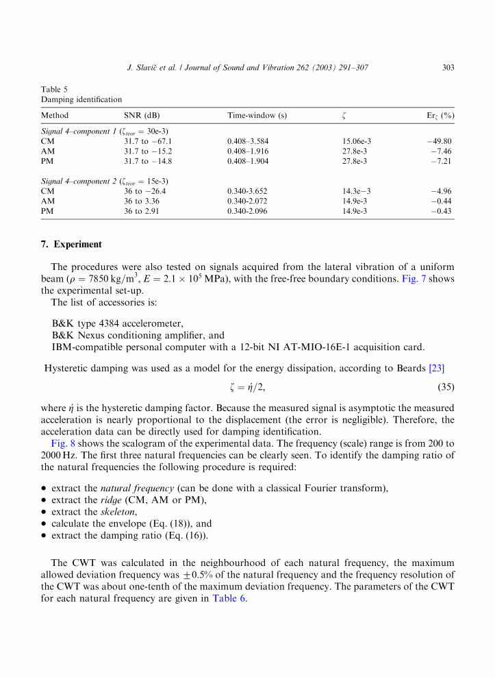
7. Experiment
The procedures were also tested on signals acquired from the lateral vibration of a uniformbeam (r ¼ 7850 kg=m3; E ¼ 2:1 105 MPa), with the free-free boundary conditions. Fig. 7 showsthe experimental set-up.
The list of accessories is:
B&K type 4384 accelerometer,B&K Nexus conditioning amplifier, andIBM-compatible personal computer with a 12-bit NI AT-MIO-16E-1 acquisition card.
Hysteretic damping was used as a model for the energy dissipation, according to Beards [23]
z ¼ !Z=2; ð35Þ
where !Z is the hysteretic damping factor. Because the measured signal is asymptotic the measuredacceleration is nearly proportional to the displacement (the error is negligible). Therefore, theacceleration data can be directly used for damping identification.
Fig. 8 shows the scalogram of the experimental data. The frequency (scale) range is from 200 to2000Hz. The first three natural frequencies can be clearly seen. To identify the damping ratio ofthe natural frequencies the following procedure is required:
* extract the natural frequency (can be done with a classical Fourier transform),* extract the ridge (CM, AM or PM),* extract the skeleton,* calculate the envelope (Eq. (18)), and* extract the damping ratio (Eq. (16)).
The CWT was calculated in the neighbourhood of each natural frequency, the maximumallowed deviation frequency was 70:5% of the natural frequency and the frequency resolution ofthe CWT was about one-tenth of the maximum deviation frequency. The parameters of the CWTfor each natural frequency are given in Table 6.
Table 5
Damping identification
Method SNR (dB) Time-window (s) z Erz (%)
Signal 4–component 1 (zteor ¼ 30e-3)
CM 31.7 to �67.1 0.408–3.584 15.06e-3 �49.80
AM 31.7 to �15.2 0.408–1.916 27.8e-3 �7.46
PM 31.7 to �14.8 0.408–1.904 27.8e-3 �7.21
Signal 4–component 2 (zteor ¼ 15e-3)
CM 36 to �26.4 0.340-3.652 14.3e�3 �4.96
AM 36 to 3.36 0.340-2.072 14.9e-3 �0.44
PM 36 to 2.91 0.340-2.096 14.9e-3 �0.43
J. Slavi $c et al. / Journal of Sound and Vibration 262 (2003) 291–307 303

The damping parameters for each natural frequency are given in Table 7. If the particularnatural frequency is present for a relatively long time, then there is usually no need to use theidentification procedures on the whole time-length. This was the case in the first two naturalfrequencies; the break point of damping identification is therefore not reached. However, by
0.00660.6666
1.32661.9866
200. 500. 800. 1100. 1400. 1700. 2000.
Time [s]
Frequency [Hz]
Wx
~309Hz
~851Hz
~1652Hz
2
Fig. 8. Scalogram of the experimental data.
Table 6
Parameters of the CWT
Natural frequency
Parameter 1st 2nd 3rd Note
Wavelet transform
f0 (Hz)E 309 851 1652 Natural frequency
s1 Hz 3 5 6 Normalized ss 99e-6 165e-6 198e-6 Parameter sDf (Hz) 0.15 0.4 0.6 Frequency resolution
uwd (ms) 25.06 15.19 9.38 Time-width
Do (Hz) 66 108 175 Band-width
Z (Hz) 30303 Frequency modulation
Fig. 7. Experiment set-up.
J. Slavi $c et al. / Journal of Sound and Vibration 262 (2003) 291–307304
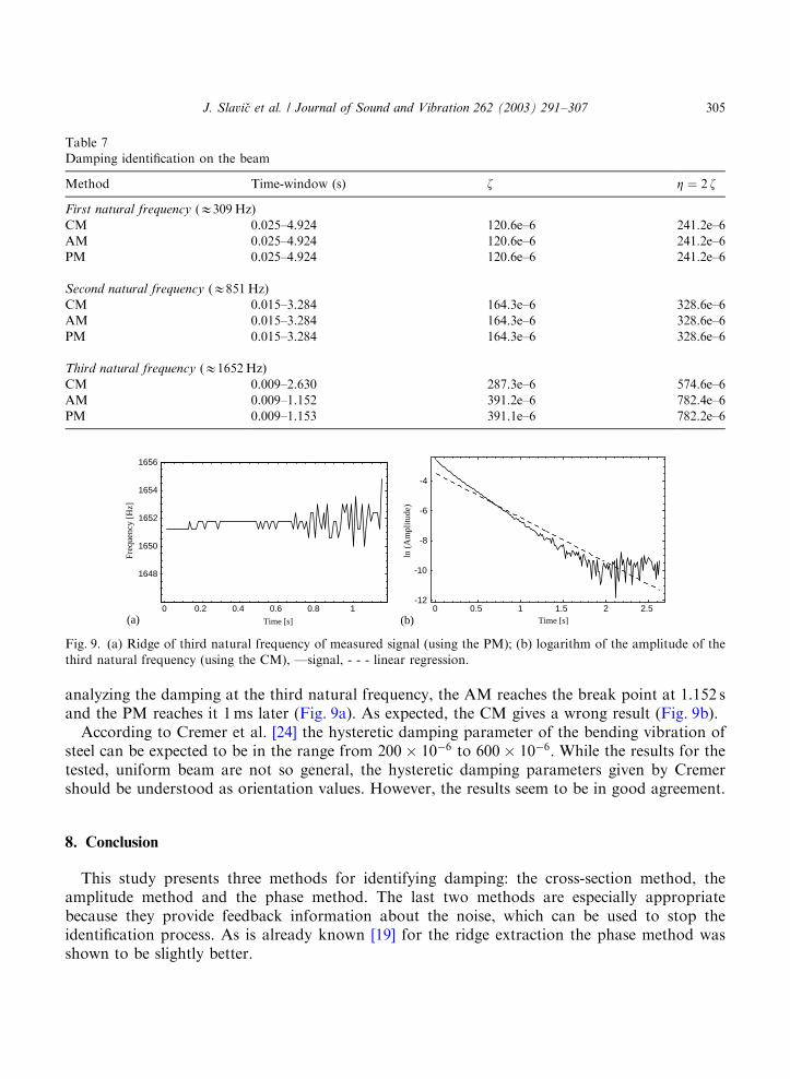
analyzing the damping at the third natural frequency, the AM reaches the break point at 1.152 sand the PM reaches it 1ms later (Fig. 9a). As expected, the CM gives a wrong result (Fig. 9b).
According to Cremer et al. [24] the hysteretic damping parameter of the bending vibration ofsteel can be expected to be in the range from 200 10�6 to 600 10�6: While the results for thetested, uniform beam are not so general, the hysteretic damping parameters given by Cremershould be understood as orientation values. However, the results seem to be in good agreement.
8. Conclusion
This study presents three methods for identifying damping: the cross-section method, theamplitude method and the phase method. The last two methods are especially appropriatebecause they provide feedback information about the noise, which can be used to stop theidentification process. As is already known [19] for the ridge extraction the phase method wasshown to be slightly better.
Table 7
Damping identification on the beam
Method Time-window (s) z Z ¼ 2 z
First natural frequency (E309 Hz)
CM 0.025–4.924 120.6e–6 241.2e–6
AM 0.025–4.924 120.6e–6 241.2e–6
PM 0.025–4.924 120.6e–6 241.2e–6
Second natural frequency (E851 Hz)
CM 0.015–3.284 164.3e–6 328.6e–6
AM 0.015–3.284 164.3e–6 328.6e–6
PM 0.015–3.284 164.3e–6 328.6e–6
Third natural frequency (E1652 Hz)
CM 0.009–2.630 287.3e–6 574.6e–6
AM 0.009–1.152 391.2e–6 782.4e–6
PM 0.009–1.153 391.1e–6 782.2e–6
0 0.2 0.4 0.6 0.8 1
1648
1650
1652
1654
1656
Time [s]
Freq
uenc
y [H
z]
0 0.5 1 1.5 2 2.5-12
-10
-8
-6
-4
Time [s]
ln (
Am
plitu
de)
(a) (b)
Fig. 9. (a) Ridge of third natural frequency of measured signal (using the PM); (b) logarithm of the amplitude of the
third natural frequency (using the CM), —signal, - - - linear regression.
J. Slavi $c et al. / Journal of Sound and Vibration 262 (2003) 291–307 305

While other authors use the Morlet wavelet function, the Gabor wavelet function was usedhere. Consequently, the approximation of the continuous wavelet transform for the asymptoticsignals was derived (Eq. (39)). The reason for choosing the Gabor wavelet function is thepossibility of adapting its time and frequency spread.
This study also treats the instantaneous SNR, which provides a better description of the noiseinfluence on the identification. It was found that the identification was still good, even with a noiseof 0 dB, although for better results the noise should be less than 5 dB.
The analytically defined time length of the edge-effect is not only important for the case ofautomating the damping identification, but it is also important if the edge-effect needs to bereduced. The parameter s of the Gabor wavelet has a critical influence on the edge-effect. A largers gives a lower frequency spread and is therefore more appropriate for analyzing close modes, aconsequence of which is a slightly better resistance to noise. However, a larger s also has somedisadvantages: because the time spread increases the reconstruction gets worse; however, the timespread does not significantly affect the logarithm of the reconstructed envelope so theidentification does not get worse. Usually, an appropriate parameter s has to be chosen, on theone hand to ensure a small edge-effect and on the other hand, to have the opportunity to analyzeclose modes and to get a good reconstruction. By choosing a small parameter s the shift of theamplitude extreme must be taken into account.
The procedures presented were also tested on a beam; the theoretical model of a damped modelbased on the hysteretic damping and the hysteretic damping factor was identified with theprocedures. The results are in accordance with the literature [24].
Appendix A. Approximation of the continuous CWT of an asymptotic signal
According to Delprat [19] a sinusoidal signal, like those presented in Eq. (8), can be representedas a real part of an analytic signal xðtÞ ¼ ReðxaðtÞÞ; where
xaðtÞ ¼ AðtÞ ei jðtÞ: ðA:1Þ
The connection between the CWT of an analytic and a real signal is Wxðu; sÞ ¼ 12Wxaðu; sÞ [14]. So
the CWT of a real signal is
Wxðu; sÞ ¼1
2
Z þN
�N
xðtÞcn
Gaboru;sðtÞ dt; ðA:2Þ
Wxðu; sÞ ¼1
2
Z þN
�N
AðtÞ eijðtÞ 1ffiffis
p 1
ðs2pÞ1=4e�ððt�uÞ=sÞ2=ð2s2Þe�iZðt�uÞ=s dt: ðA:3Þ
First substitute the time t ¼ t þ u; then use the Taylor power series expansion close to u: for theamplitude of order 0: Aðt þ uÞ ¼ AðuÞ; and for the phase of order 1: jðt þ uÞ ¼ jðuÞ þ j0ðuÞðt � uÞ:After the integration the following expression is obtained:
Wxðu; sÞ ¼ 12 AðuÞ #cGaboru;sðj
0ðuÞ; s; ZÞ ei jðuÞ þ Er A0ðtÞ;j00ðuÞ� �
: ðA:4Þ
Because of the Taylor expansion the generality is lost; however, if the frequency dissipation of thewavelet function is relatively small then the error Er A0ðtÞ;j00ðuÞð Þ can be neglected (Eq. (11)) [14].
J. Slavi $c et al. / Journal of Sound and Vibration 262 (2003) 291–307306
References
[1] W.T. Thomson, Theory of Vibration with Applications, 4th edition, Chapman & Hall, London, 1993.
[2] R.B. Randall, Vibration measurement equipment and signal analyzers, in: C.M. Harris (Ed.), Shock and Vibration
Handbook, 3rd edition, McGraw-Hill, New York, 1987.
[3] A.D. Nashif, D.I.G. Jones, J.P. Henderson, Vibration Damping, 2nd edn, Wiley, New York, 1985.
[4] W.J. Staszewski, Identification of damping in mdof systems using time-scale decomposition, Journal of Sound and
Vibration 203 (1997) 283–305.
[5] M. Bolte$zar, I. Simonovski, M. Furlan, Fault detection in DC electro motors using the continuous wavelet
transform, Meccanica, in press.
[6] I. Simonovski, Val$cna Analiza Nelinearnih Nestacionarnih Nihanj Elektromotorja, Wavelet Analysis of Nonlinear
and Non-stationary Electro-motor Vibrations, Ph.D. Thesis, Slovene.
[7] I. Simonovski, M. Bolte$zar, Monitoring the instantaneous frequency content of a washing machine during startup,
Strojni$ski vestnik–Journal of Mechanical Engineering 47 (2001) 28–44.
[8] P. Argoul, H.P. Yin, B. Guillermin, Use of the wavelet transform for the processing of mechanical signals,
Proceedings of the 23rd ISMA Conference, Leuven, Vol. 1, Belgique, 1998, pp. 375–403.
[9] H.P. Yin, P. Argoul, Integral transforms and modal identification, Comptes Rendus Academie Sciences de Paris
327 (IIb) (1999) 777–783.
[10] C.H. Lamarque, S. Pernot, A. Cuer, Damping identification in multi-degree-of-freedom systems via a wavelet-
logarithmic decrement—part 1: theory, Journal of Sound and Vibration 235 (2000) 361–374.
[11] S. Hans, E. Ibraim, S. Pernot, C. Boutin, C.H. Lamarque, Damping identification in multi-degree-of-freedom
systems via a wavelet-logarithmic decrement—part 2: study of a civil engineering building, Journal of Sound and
Vibration 235 (2000) 375–403.
[12] P. Argoul, S. Hans, F. Conti, C. Boutin, Time-frequency analysis of free oscillations of mechanical structures.
Application to the identification of the mechanical behavior of buildings under shocks, in: J.A. Gemes (Ed.),
COST F3 Conference: System Identification and Structural Health Monitoring, Universidad Polit"ecnica de
Madrid, Madrid, 2001, pp. 283–292.
[13] J. Slavi$c, Identifikacija Du$senja Nihajo$cih Sistemov z Ve$c Prostostnimi Stopnjami z Uporabo Val$cne
Transformacije, Identification of Damping in Multi-degree-of-freedom Systems using Wavelet Transformation,
Graduation Thesis, 2001, Slovene.
[14] S. Mallat, A Wavelet Tour of Signal Processing, 2nd edition, Academic Press, New York, 1999.
[15] C. Torrence, G.P. Compo, A practical guide to wavelet analysis, Bulletin of the America Meteorological Society 79
(1998) 61–78.
[16] A. Grossman, J. Morlet, Decomposition of hardy function into square integrable wavelets of constant shape,
SIAM Journal of Mathematical Analysis and Applications 15 (1984) 723–736.
[17] P. Tchamitchian, B. Torresani, Ridge and skeleton extraction from the wavelet transform, in: M.B. Ruskai (Ed.),
Wavelets and Their Applications, Jones and Bartlett, Boston, 1992, pp. 123–151.
[18] M. Ruzzene, A. Fasana, L. Garibaldi, B. Piombo, Natural frequencies and dampings identification using wavelet
transform: Application to real data, Mechanical Systems and Signal Processing 11 (1997) 207–218.
[19] N. Delprat, B. Escudie, P. Guillemain, R.K. Martinet, Ph. Tchamitchian, B. Torresani, Asymptotic wavelet and
Gabor analysis: extraction of instantaneous frequencies (special issue on Wavelet and Multiresolution Analysis),
IEEE Transactions on Information Theory 38 (1992) 644–664.
[20] R.A. Carmona, W.L. Hwang, B. Torresani, Characterization of signals by the ridges of their wavelet transform,
IEEE Transactions on Signal Processing 45 (1997) 2586–2590.
[21] K. Worden, Data processing and experiment design for the restoring force surface method, part 1: integration and
differentiation of measured time data, Mechanical Systems, Signal Processing 4 (1990) 295–319.
[22] I. Grabec, J. Gradi$sek, Opis naklju$cnih pojavov, Random data analysis, Fakulteta za strojni$stvo, Ljubljani,
Slovene, 2000.
[23] C.F. Beards, Structural Vibration: Analysis and Damping, Arnold, Paris, 1996.
[24] L. Cremer, M. Heckl, Structure-Borne Sound, Springer, Berlin, 1973, pp. 205–217 (Chapter III).
J. Slavi $c et al. / Journal of Sound and Vibration 262 (2003) 291–307 307