SRI/USEPA-GHG-QAP-24 March 2004

Test and Quality Assurance Plan Electric Power and Heat Production Using Renewable Biogas at a Dairy Farm

Prepared by:

Greenhouse Gas Technology Center Southern Research Institute

Under a Cooperative Agreement With U.S. Environmental Protection Agency

and

Under Agreement With New York State Energy and Research Development Authority

EPA REVIEW NOTICE

This report has been peer and administratively reviewed by the U.S. Environmental Protection Agency, and approved for publication. Mention of trade names or commercial products does not constitute endorsement or recommendation for use.

SRI/USEPA-GHG-QAP-24 March 2004

Greenhouse Gas Technology Center A U.S. EPA Sponsored Environmental Technology Verification ( ) Organization

Test and Quality Assurance Plan

Electric Power and Heat Production Using Renewable Biogas at a Dairy Farm

Prepared by: Greenhouse Gas Technology Center

Southern Research Institute PO Box 13825

Research Triangle Park, NC 27709 USA Telephone: 919/806-3456

Reviewed by:

New York State Electric and Gas Corporation New York State Energy Research and Development Authority

Dairy Development International U.S. EPA Office of Research and Development QA Team

indicates comments are integrated into Test Plan

Greenhouse Gas Technology Center A U.S. EPA Sponsored Environmental Technology Verification ( ) Organization

Test and Quality Assurance Plan

Electric Power and Heat Production Using Renewable Biogas at a Dairy Farm

This Test and Quality Assurance Plan has been reviewed and approved by the Greenhouse Gas Technology Center Project Manager and Director, the U.S. EPA APPCD Project Officer, and the U.S. EPA APPCD Quality Assurance Manager.

Signed 3/18/04 Signed 3/18/04 Stephen Piccot Date David Kirchgessner Date Director APPCD Project Officer Greenhouse Gas Technology Center U.S. EPA Southern Research Institute

SignedWilliam Chatterton Project Manager Greenhouse Gas Technology Center Southern Research Institute

3/18/04 Signed 3/18/04 Date Robert S. Wright Date

APPCD Quality Assurance Manager U.S. EPA

Test Plan Final: March 2004

TABLE OF CONTENTS Page

Appendices ................................................................................................................................................List of Figures ................................................................................................................................................List of Tables ................................................................................................................................................Distribution List ................................................................................................................................................Acronyms/Abbreviations ..................................................................................................................................

1.0 INTRODUCTION .................................................................................................................................1-11.1 BACKGROUND ..........................................................................................................................1-11.2 TEST FACILITY DESCRIPTION ...............................................................................................1-31.3 MICROTURBINE CHP SYSTEM TECHNOLOGY DESCRIPTION........................................1-61.4 ORGANIZATION ........................................................................................................................1-81.5 SCHEDULE................................................................................................................................1-10

2.0 VERIFICATION APPROACH............................................................................................................2-12.1 OVERVIEW OF CHP SYSTEM PERFORMANCE TESTING..................................................2-12.2 POWER AND HEAT PRODUCTION PERFORMANCE ..........................................................2-4

2.2.1 Electric Power Output and Efficiency Determination......................................................2-42.2.2 Heat Recovery Rate and Thermal Efficiency Determination...........................................2-72.2.3 Measurement Instruments ................................................................................................2-8

2.2.3.1 Power Output Measurements ...........................................................................2-82.2.3.2 Gas Flow Meter ................................................................................................2-92.2.3.3 Gas Temperature and Pressure Measurements .................................................2-92.2.3.4 Gas Composition and Heating Value Analysis ................................................2-92.2.3.5 Fuel Moisture Analysis ..................................................................................2-102.2.3.6 Ambient Conditions Measurements ...............................................................2-112.2.3.7 Heat Recovery Rate Measurements................................................................2-11

2.3 POWER QUALITY PERFORMANCE .....................................................................................2-122.3.1 Electrical Frequency ......................................................................................................2-132.3.2 Generator Line Voltage..................................................................................................2-132.3.3 Voltage Total Harmonic Distortion ...............................................................................2-132.3.4 Current Total Harmonic Distortion................................................................................2-142.3.5 Power Factor ..................................................................................................................2-152.3.6 Power Quality Measurement Instruments ......................................................................2-15

2.4 EMISSIONS PERFORMANCE .................................................................................................2-152.4.1 Stack Emission Rate Determination...............................................................................2-152.4.2 Gaseous Sample Conditioning and Handling ................................................................2-162.4.3 Gaseous Pollutant Sampling Procedures........................................................................2-172.4.4 Determination of Emission Rates...................................................................................2-192.4.5 Total Particulate (TPM) Emissions Sampling and Analysis procedures .......................2-20

2.5 ELECTRICITY OFFSETS AND ESTIMATION OF EMISSION REDUCTIONS ..................2-212.5.1 Microturbine CO2 and NOX Emissions Estimation .......................................................2-222.5.2 Estimation of Electric Grid Emissions ...........................................................................2-22

3.0 DATA QUALITY ..................................................................................................................................3-13.1 BACKGROUND ..........................................................................................................................3-13.2 ELECTRICAL POWER OUTPUT AND POWER QUALITY ...................................................3-23.3 EFFICIENCY................................................................................................................................3-6

3.3.1 Fuel Gas Flow Rate Quality Assurance ...........................................................................3-73.3.2 Gas Pressure and Barometric Pressure Quality Assurance ..............................................3-8

i

3.3.3 Gas Temperature and Ambient Temperature Quality Assurance ....................................3-83.3.4 Fuel Gas Analyses Quality Assurance .............................................................................3-83.3.5 Heat Recovery Rate Quality Assurance ...........................................................................3-9

3.4 EMISSION MEASUREMENTS QA/QC PROCEDURES ..........................................................3-93.4.1 NOx Emissions Quality Assurance...................................................................................3-93.4.2 CO, CO2, O2, and SO2 Emissions Quality Assurance ....................................................3-113.4.3 CH4, NH3, and TRS Emissions Quality Assurance........................................................3-143.4.4 Gas Flow Rate and Particulate Emissions Quality Assurance .......................................3-15

3.5 INSTRUMENT TESTING, INSPECTION, AND MAINTENANCE .......................................3-173.6 INSPECTION/ACCEPTANCE OF SUPPLIES AND CONSUMABLES.................................3-17

4.0 DATA ACQUISITION, VALIDATION, AND REPORTING..........................................................4-14.1 DATA ACQUISITION AND STORAGE....................................................................................4-1

4.1.1 Continuous Measurements ...............................................................................................4-14.1.2 Emission Measurements ..................................................................................................4-44.1.3 Off Site Analyses .............................................................................................................4-4

4.2 DATA REVIEW, VALIDATION, AND VERIFICATION.........................................................4-54.3 RECONCILIATION OF DATA QUALITY OBJECTIVES........................................................4-54.4 ASSESSMENTS AND RESPONSE ACTIONS ..........................................................................4-6

4.4.1 Project Reviews ...............................................................................................................4-64.4.2 Inspections .......................................................................................................................4-64.4.3 Performance Evaluation Audit.........................................................................................4-74.4.4 Technical Systems Audit .................................................................................................4-74.4.5 Audit of Data Quality.......................................................................................................4-7

4.5 DOCUMENTATION AND REPORTS .......................................................................................4-84.5.1 Field Test Documentation ................................................................................................4-84.5.2 QC Documentation ..........................................................................................................4-84.5.3 Corrective Action and Assessment Reports .....................................................................4-84.5.4 Verification Report and Verification Statement ..............................................................4-9

4.6 TRAINING AND QUALIFICATIONS .....................................................................................4-104.7 HEALTH AND SAFETY REQUIREMENTS ...........................................................................4-10

5.0 REFERENCES ......................................................................................................................................5-1

ii

APPENDICES Page

APPENDIX A Test Procedures and Field Log Forms ............................................................. A-1

LIST OF FIGURES Page

Figure 1-1 Photograph of the DDI Farm ............................................................................ 1-3 Figure 1-2 Schematic of the Biogas production and Use Process ...................................... 1-4 Figure 1-3 Capstone CHP System Process Diagram .......................................................... 1-7 Figure 1-4 Project Organization ......................................................................................... 1-9 Figure 2-1 Schematic of Measurement System .................................................................. 2-4 Figure 2-2 Gaseous Pollutant Sampling System............................................................... 2-17 Figure 4-1 DAS Schematic ................................................................................................. 4-2

LIST OF TABLES Page

Table 1-1 Capstone Microturbine Model 330 Specifications............................................ 1-8 Table 2-1 Verification Test Matrix.................................................................................... 2-3 Table 2-2 Permissible Variations in Power, Fuel, and Atmospheric Conditions .............. 2-5 Table 2-3 Target Set-Points for Heat Recovery Unit ........................................................ 2-7 Table 2-4 Summary of Emission Testing Methods ......................................................... 2-16 Table 2-5 CO2 and COX Emission Rates for Two Geographical Regions ...................... 2-24 Table 3-1 Verification Parameter DQOs ........................................................................... 3-1 Table 3-2 Measurement Instrument Specification and DQI Goals ................................... 3-3 Table 3-3 Summary of QA/QC Checks............................................................................. 3-5 Table 3-4 Electrical Efficiency Error Propagation and DQOs .......................................... 3-7 Table 3-5 ASTM D1945 Repeatability Specifications.................................................... 3-10 Table 3-6 Instrument Specifications and DQI Goals for Stack Emissions Testing......... 3-12 Table 3-7 Summary of Emissions Testing Calibrations and QC Checks ........................ 3-13 Table 4-1 Continuous Data to be Collected for CHP System Evaluation ......................... 4-3

iii

ACRONYMS/ABBREVIATIONS

Abs. Diff. absolute difference AC alternating current ADQ Audit of Data Quality amps amperes ANSI American National Standards Institute APPCD Air Pollution Prevention and Control Division ASHRAE American Society of Heating, Refrigerating and Air-Conditioning Engineers, Inc. ASME American Society of Mechanical Engineers Btu British thermal units Btu/hr British thermal units per hour Btu/lb British thermal units per pound Btu/min British thermal units per minute Btu/scf British thermal units per standard cubic foot C1 quantification of methane C6+ hexanes plus CAR Correction Action Report CH4 methane CHP combined heat and power CO carbon monoxide CO2 carbon dioxide CT current transformer DAS data acquisition system DG distributed generation DMM digital multimeter DOE U.S. Department of Energy DP differential pressure DQI data quality indicator DQO data quality objective dscf/MMBtu dry standard cubic feet per million British thermal units EIA Energy Information Administration EPA Environmental Protection Agency ETV Environmental Technology Verification °C degrees Celsius oF degrees Fahrenheit FERC Federal Energy Regulatory Commission FID flame ionization detector fps ft3

feet per second cubic feet

gal U.S. gallons GC gas chromatograph GHG Center Greenhouse Gas Technology Center gpm gallons per minute GU generating unit

(continued)

iv

ACRONYMS/ABBREVIATIONS (continued)

hr hour Hz hertz IC internal combustion IEEE Institute of Electrical and Electronics Engineers IPCC Intergovernmental Panel on Climate Change kVA kilovolt-ampere kVAr kilovolt reactive kW kilowatt kWh kilowatt hour kWh/yr kilowatt hour per year lb pound lb/Btu pounds per British thermal unit lb/dscf lb/ft3

pounds per dry standard cubic foot pounds per cubic foot

lb/hr pounds per hour lb/kWh pounds per kilowatt-hour lb/yr pounds per year ISO International Standards Organization LHV lower heating value MMBtu/hr million British thermal units per hour MMcf million cubic feet mol molecular N2 nitrogen NDIR nondispersive infrared NIST National Institute of Standards and Technology NOX nitrogen oxides NSPS New Source Performance Standards NYSEG New York State Electric and Gas Corporation NYSERDA New York State Energy Research and Development Authority O2 oxygen ORD Office of Research and Development PEA Performance Evaluation Audit ppmv parts per million volume ppmvd parts per million volume dry psia pounds per square inch absolute psig pounds per square inch gauge PT potential transformer QA/QC Quality Assurance/Quality Control QMP Quality Management Plan Rel. Diff. relative difference Report Environmental Technology Verification Report RH relative humidity rms root mean square

(continued)

v

ACRONYMS/ABBREVIATIONS (continued)

rpm revolutions per minute RTD resistance temperature detector scfh standard cubic feet per hour scfm standard cubic feet per minute SRI Southern Research Institute T&D transmission and distribution Test Plan Test and Quality Assurance Plan THCs total hydrocarbons THD total harmonic distortion TPM total particulate matter TRS total reduced sulfur TSA technical systems audit U.S. United States VAC volts alternating current WRAP Western Regional Air Partnership WRI World Resources Institute

vi

DISTRIBUTION LIST

New York State Energy Research and Development Authority (NYSERDA) Richard Drake Joe Sayer

Tom Friesinger

New York State Gas and Electric Company (NYSEG) Bruce Roloson

Jim Harvilla

Dairy Development International, LLC (DDI) Larry Jones

U.S. EPA – Office of Research and Development David Kirchgessner

Robert S. Wright

Southern Research Institute (GHG Center) Stephen Piccot William Chatterton

Robert G. Richards Ashley Williamson

vii

(this page intentionally left blank)

viii

1.0 INTRODUCTION

1.1 BACKGROUND

The U.S. Environmental Protection Agency’s Office of Research and Development (EPA-ORD) operates the Environmental Technology Verification (ETV) program to facilitate the deployment of innovative technologies through performance verification and information dissemination. The goal of the ETV program is to further environmental protection by substantially accelerating the acceptance and use of improved and innovative environmental technologies. Congress funds ETV in response to the belief that there are many viable environmental technologies that are not being used for the lack of credible third­party performance data. With performance data developed under this program, technology buyers, financiers, and permitters in the United States and abroad will be better equipped to make informed decisions regarding environmental technology purchase and use.

The Greenhouse Gas Technology Center (GHG Center) is one of six verification organizations operating under the ETV program. The GHG Center is managed by EPA’s partner verification organization, Southern Research Institute (SRI), which conducts verification testing of promising GHG mitigation and monitoring technologies. The GHG Center’s verification process consists of developing verification protocols, conducting field tests, collecting and interpreting field and other data, obtaining independent peer-review input, and reporting findings. Performance evaluations are conducted according to externally reviewed verification Test and Quality Assurance Plans (Test Plan) and established protocols for quality assurance (QA).

The GHG Center is guided by volunteer groups of stakeholders. These stakeholders offer advice on specific technologies most appropriate for testing, help disseminate results, and review Test Plans and Technology Verification Reports (Report). The GHG Center’s Executive Stakeholder Group consists of national and international experts in the areas of climate science and environmental policy, technology, and regulation. It also includes industry trade organizations, environmental technology finance groups, governmental organizations, and other interested groups. The GHG Center’s activities are also guided by industry specific stakeholders who provide guidance on the verification testing strategy related to their area of expertise and peer-review key documents prepared by the GHG Center.

One technology of interest to some GHG Center stakeholders is distributed electrical power generation systems. Distributed generation (DG) refers to equipment, typically ranging from 5 to 1,000 kilowatts (kW) that provide electric power at a site closer to customers than central station generation. A distributed power unit can be connected directly to the customer or to a utility’s transmission and distribution (T&D) system. Examples of technologies available for DG includes gas turbine generators, internal combustion (IC) engine generators (gas, diesel, other), photovoltaics, wind turbines, fuel cells, and microturbines. DG technologies provide customers one or more of the following main services: standby generation (i.e., emergency backup power), peak shaving generation (during high demand periods), baseload generation (constant generation), or cogeneration [combined heat and power (CHP) generation].

Recently, biogas production from livestock manure management facilities has become a promising alternative to fueling DG technologies. EPA estimates U.S. methane (CH4) emissions from livestock manure management (the primary constituent in biogas) to be 17.0 million tons carbon equivalent. This accounts for almost 10 percent of total 1997 CH4 emissions in the country (EPA 1999a). The majority of CH4 emissions come from large swine and dairy farms that manage manure as a liquid. The EPA expects

1-1

U.S. CH4 emissions from livestock manure to grow by over 25 percent from 2000 to 2020. Cost effective manure management systems are available that can stem this emission growth by recovering CH4 and using it as an energy source. These systems, commonly referred to as anaerobic digesters, decompose manure in a controlled environment and recover CH4 produced from the manure. The recovered CH4 serves as fuel to power generators that produce on-site electricity, heat, and hot water. Digesters also reduce foul odor and can reduce the risk of ground- and surface-water pollution.

Several states including New York, Colorado, and California are exploring technology solutions to address each state’s manure waste management, odor, and water discharge problems, and have identified anaerobic digesters, coupled with DG technologies as a viable option. The GHG Center and the New York State Energy Research and Development Authority (NYSERDA) have agreed to collaborate and share the cost of verifying several new DG technologies throughout the State of New York. One such technology consists of a series of microturbines that operate on biogas recovered from a dairy farm anaerobic digestion process in Homer, NY. This verification will evaluate the performance of four 30 kW microturbines coupled with a single heat recovery system offered by Capstone Turbine Corporation (Capstone). The cost to conduct this verification is being funded jointly by EPA’s ETV program and NYSERDA.

The Capstone CHP system is currently being installed at a farm operated by Dairy Development International (DDI), and is part of a joint project between NYSERDA, DDI, and the New York State Gas and Electric Corporation (NYSEG). The CHP system will operate on biogas and will be interconnected to the electric utility grid. The site does not anticipate exporting power for sale since all of the electricity generated can be consumed on-site. Heat will be recovered according to the site’s thermal demand (i.e., heat digester, heat barn floors), and any unused heat will be discarded from the CHP system exhaust stack. The overall energy conversion efficiency is estimated to range between 50 and 75 percent, which is high enough to significantly reduce greenhouse gas (GHG) emissions, and provide end users with a renewable source of energy.

Field tests will be performed to independently verify the electricity generation rate, heat recovery rate, electrical power quality, energy efficiency, conventional and criteria air pollutant emissions, and GHG emission reductions from offsetting electricity generation from the utility grid.

This document is the Test Plan for performance verification of the Capstone CHP system at DDI. It contains the rationale for the selection of verification parameters, the verification approach, data quality objectives (DQOs), and Quality Assurance/Quality Control procedures (QA/QC), and will guide implementation of the test, creation of test documentation, data analysis, and interpretation.

This Test Plan has been reviewed by NYSERDA, DDI, NYSEG, and the EPA QA team. Once approved, as evidenced by the signature sheet at the front of this document, it will meet the requirements of the GHG Center’s Quality Management Plan (QMP) and thereby satisfy the ETV QMP requirements. The final Test Plan will be posted on the Web sites maintained by the GHG Center (www.sri-rtp.com) and the ETV program (www.epa.gov/etv).

Upon field test completion, the GHG Center will prepare a Report and Verification Statement. The Report and the Verification Statement will be reviewed by the same organizations listed above, followed by EPA-ORD technical review. When this review is complete, the GHG Center Director and EPA-ORD Laboratory Director will sign the Verification Statement, and the final documents will be posted on the GHG Center and ETV program Web sites.

The following section provides a description of the microturbine CHP technology and the DDI farm facility. This is followed by a list of performance verification parameters that will be quantified through

1-2

independent testing at the site. The section concludes with a discussion of key organizations participating in this verification, their roles, and the verification test schedule. Section 2.0 describes the technical approach for verifying each parameter, including sampling, analytical, and QA/QC procedures. Section 3.0 identifies the data quality assessment criteria for critical measurements and states the accuracy, precision, and completeness goals for each measurement. Section 4.0 discusses data acquisition, validation, reporting, and auditing procedures.

1.2 TEST FACILITY DESCRIPTION

The DDI facility is a newly constructed 850-cow dairy farm in Homer, New York. Ground was broken for the facility in February 2001, and milk production began in August 2001. Figure 1-1 is a photograph of the farm, and Figure 1-2 shows a biogas generation and use process schematic. Dairy cows are housed in two free-stall barns which are 438 feet long and 96 feet wide (Figure 1-2). The barns are designed to ensure that manure does not escape from the alleys. Mechanical alley scrapers automatically and continuously scrape the manure to center flow gutters, where the manure enters a gravity flow system. The barn floors are equipped with a heating system to ensure that the alley scrapers work during freezing weather.

Free-stall Anaerobic Solids/Liquid Liquid Manure Storage Separator Digester Barns Parlor, Milk Special

House Needs Barn Building

Figure 1-1. Photograph of the DDI Farm

The manure from the barn floors is moved to a concrete gutter in the middle of each barn. The gutters are connected by a double walled plastic pipe. The farm was built with a one-foot drop in elevation between barns, where step dams are placed to ensure manure mixing. The manure from the free-stall barns and the wastewater from the milk house are collected in a 17,000 gallon concrete collection pit, where the solids content is monitored to ensure a maximum concentration of 12 percent. From the collection pit, manure is pumped through a 6-inch polyvinyl chloride (PVC) line to the anaerobic digester. This system is a plug

1-3

LivestockHousing

AnaerobicDigester

SeparatorBuilding

UnifinHt. Exch.

C330 C330

BiogasTreatment

System

LivestockHousing

AnaerobicDigester

SeparatorBuilding

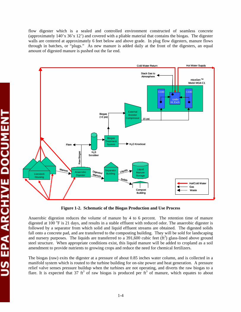
flow digester which is a sealed and controlled environment constructed of seamless concrete (approximately 140’x 36’x 12’) and covered with a pliable material that contains the biogas. The digester walls are centered at approximately 6 feet below and above grade. In plug flow digesters, manure flows through in batches, or “plugs.” As new manure is added daily at the front of the digesters, an equal amount of digested manure is pushed out the far end.

Cold Water ReturnCold Water Return

Raw

Bio

gas

External Booster

Compressor

H2S Scrubber

15 psi

Manure DigestedManure

Liquid Manure Storage

Compost Building

Liquids

Solids

Flare

Hot Water Supply

Stack Gas to Atmosphere

micoGen TM

Model MG4-C1

Hot/Cold Water Gas Waste

H2O Knockout

Biogas (<2 psi)

Raw

Bio

gas

ExternalBooster

Compressor

ExternalBooster

Compressor

H2SScrubber

15 psi

Livestock Housing

Anaerobic Digester

Manure Separator Building

DigestedManure

LiquidManureStorage

LiquidManureStorage

CompostBuilding

Liquids

Solids

Flare

Hot Water Supply

Stack Gas toAtmosphere

Unifin Ht. Exch.

C330 C330

micoGen TM

Model MG4-C1

Hot/Cold WaterGasWaste

Biogas Treatment

System H2O Knockout

Biogas(<2 psi)

Figure 1-2. Schematic of the Biogas Production and Use Process

Anaerobic digestion reduces the volume of manure by 4 to 6 percent. The retention time of manure digested at 100 oF is 21 days, and results in a stable effluent with reduced odor. The anaerobic digester is followed by a separator from which solid and liquid effluent streams are obtained. The digested solids fall onto a concrete pad, and are transferred to the composting building. They will be sold for landscaping and nursery purposes. The liquids are transferred to a 391,600 cubic feet (ft3) glass-lined above ground steel structure. When appropriate conditions exist, this liquid manure will be added to cropland as a soil amendment to provide nutrients to growing crops and reduce the need for chemical fertilizers.

The biogas (raw) exits the digester at a pressure of about 0.85 inches water column, and is collected in a manifold system which is routed to the turbine building for on-site power and heat generation. A pressure relief valve senses pressure buildup when the turbines are not operating, and diverts the raw biogas to a flare. It is expected that 37 ft3 of raw biogas is produced per ft3 of manure, which equates to about

1-4

110,000 ft3 per day raw biogas production at the test site. The biogas production rate variability over time (e.g., days, years) is unknown since the DDI dairy operation is relatively new. Based on a comprehensive report published for a plug flow anaerobic digestion facility in Minnesota, an average daily biogas recovery rate from 430 dairy cows for about 1 year of operation was documented to be 59,000 ft3/day ± 2 percent (Nelson and Lamb 2000). The DDI farm manages two times as many cows, and has reported a production rate that is almost twice as large as the Minnesota farm (110,000 ft3/day). Based on this and the similarity in waste management techniques of the two dairy operations, it is expected that the potential gas recovery rate and variability will be similar.

The primary gas constituents of the raw biogas are CH4 (around 60 %) and CO2 (approximately 37 %). It also contains trace amounts of ammonia (NH3), hydrogen sulfide (H2S), mercaptans, and other noxious gases, and is likely to be saturated with water vapor. The lower heating value (LHV) of the biogas is approximately 600 Btu/scf.

To make use of the available biogas, DDI and NYSEG process the raw gas to remove impurities (i.e., water, CO2, and H2S). The site’s layout and topography will assist moisture removal from the raw biogas. Approximately 800 feet of underground piping buried below the frost line carries the biogas to the microturbines. This distance and the relatively constant ground temperature (approximately 50 °F) allows water in the biogas to condense naturally. The condensed liquid returns to the digester through the inclined pipeline. The site also uses two desiccant dryers in series for additional moisture removal.

The dry biogas is then directed to H2S scrubber where that is designed to reduce H2S concentrations to 1,000 ppm or less. The scrubber is an iron sponge that consists of wood shavings or chips that are impregnated with hydrated iron oxide. In the iron sponge, gas flows through the dry media in a low pressure vessel. The wood chips increase the bed porosity and reduce the pressure drop across the bed. The H2S in the gas stream reacts with the iron oxide to produce iron sulfide and water as shown below.

2Fe2O3 + 2H2O + 6H2S → 2Fe2S3 + 8H2O

Infused with these contaminants, the iron sponge is referred to as spent iron sponge. The spent iron sponge (iron sulfide) can be re-oxidized with exposure to air to form iron oxide and elemental sulfur according to the following reaction.

2Fe2S3 + 3O2 → 2Fe2O3 + 6S(s)

The spent media will be regenerated by filling the vessel with water, passing air through the bed, and converting the iron sulfide back to iron oxide and elemental sulfur. The media can be regenerated until it gets coated with elemental sulfur, which can block the media and increase the pressure drop across the bed. The spent media regains 50 to 60 percent of its original capacity after regeneration, and can be regenerated 2 to 3 times during its life of about 3 years. After its useful life, the wood chips will be ground up, mixed with the solid waste compost, and sold as fertilizer. Several facilities in California have successfully used the iron sponge process to reduce H2S concentrations to about 1,000 ppm. This technique is also used to remove H2S from sour gas in oil and natural gas processing operations.

The microturbine system to be verified at the dairy farm consists of two 30 kW Capstone MicroTurbines™ Model 330 and a single heat recovery system developed by Unifin International, titled micoGen™ Model MG4-C1. Both microturbines are equipped with combustors manufactured by Capstone that are designed for low-Btu gas (> 350 Btu/scf) and high H2S content (< 7 percent by volume). The CHP system requires a minimum heat input of about 377,000 Btu/hr (LHV basis) for each microturbine. This is equivalent to a total biogas flow rate of 30,160 standard cubic feet per day (scfd) for both microturbines, assuming LHV of 600 Btu/scf. The microturbines require a fuel pressure of 52 to

1-5

55 psig, so the facility has installed a gas compressor to boost biogas pressure to that level. The daily fuel consumption of the microturbines is well below the average daily raw biogas production rate. Excess biogas, unused by the microturbines, will be flared on-site. At full load, between 45 and 60 kW electrical power will be generated. The peak demand of the site is about 120 kW, and the annual average electrical power requirement is 65 kW.

The following section describes the electrical power and heat production system at the DDI farm.

1.3 MICROTURBINE CHP SYSTEM TECHNOLOGY DESCRIPTION

Natural-gas-fired turbines have been used to generate electricity since the 1950s. Technical and manufacturing developments in the last decade have enabled the introduction of microturbines with generation capacity ranging from 30 to 200 kW. Microturbines have evolved from automotive and truck turbocharger technology and small jet engine technology. A microturbine consists of a compressor, combustor, recuperator, and generator. They have a small number of moving parts, and their compact size enables them to be located on sites with limited space. For sites with thermal demands, a waste heat recovery system can be integrated with a microturbine to achieve higher efficiencies.

Although natural gas has been the primary choice of fuel for most applications, operators are increasingly examining the applicability of this technology to biogas recovered from animal waste, landfills, and wastewater treatment facilities. The availability of “free” fuel in the agricultural sector, particularly for swine and dairy operations, may offer a cost effective means of meeting odor regulations while simultaneously generating electricity and heat to offset a site’s energy demand.

Figure 1-3 illustrates a simplified process flow diagram of the CHP system, and a discussion of each component follows. Table 1-1 summarizes key operational and performance characteristics reported by Capstone. Electric power is generated from a high-speed, single shaft, recuperated turbine generator with a nominal power output of 30 kW (59 oF, sea level). Table 1-1 summarizes the physical and electrical specifications for a Capstone Model 330 microturbine. Each microturbine also consists of an air compressor, recuperator, combustor, turbine, and a permanent magnet generator as shown in Figure 1-3.

The recuperator is a heat exchanger that recovers some of the heat from the exhaust stream and transfers it to the incoming compressed air stream. The preheated air is then mixed with the fuel, and this compressed fuel/air mixture is burned in the combustor under constant pressure conditions. The resulting hot gas is allowed to expand through the turbine section to perform work, rotating the turbine blades to turn a generator, which produces electricity. Because of the inverter-based electronics that enable the generator to operate at high speeds and frequencies, the need for a gearbox and associated moving parts is eliminated. The rotating components are mounted on a single shaft, supported by patented air bearings that rotate at over 96,000 revolutions per minute (rpm) at full load. The exhaust gas exits the turbine and enters the recuperator, which pre-heats the air entering the combustor, to improve the efficiency of the system. The exhaust gas then exits the recuperator into a Unifin heat recovery unit.

The permanent magnet generator produces high frequency alternating current, (AC) which is rectified, inverted, and filtered by the line power unit into conditioned 480 volts alternating current (VAC). Each unit supplies a variable electrical frequency of 50 or 60 hertz (Hz), and is supplied with a control system, which allows for automatic and unattended operation. An active filter in the turbine is reported by the turbine manufacturer to provide cleaner power, free of spikes and unwanted harmonics. All operations, including startup, setting of programmable interlocks, grid synchronization, operational setting, dispatch, and shutdown, can be performed manually or remotely using an internal power controller system.

1-6

Combustor

On-Board Blower

ToTo

StackStack

UnifiUnifi

Hot Water Supply

Exhaust

Atmosphere

Cold Water Return

Air Inlet ~Compressor Turbine

Biogas, 15 psig

480 Volts (AC) 3 Ph, 63 A, 60 Hz

To Switchgear

Recuperator

n micoGen Model MG4

Fuel, 55 psig

Exhaust gas from both Microturbines enters the Heat exchanger

Hot WaterSupply

Exhaust

Atmosphere

Cold WaterReturn

Air Inlet~Compressor

Combustor

Turbine

Biogas, 15 psig

480 Volts (AC)3 Ph, 63 A,60 Hz

To Switchgear

Recuperator

n micoGen Model MG4

On-Board Blower

Fuel, 55 psig

Exhaust gas from bothMicroturbines enters theHeat exchanger

Capstone Model 330 MicroturbineCapstone Model 330 Microturbine

Figure 1-3. Capstone CHP System Process Diagram

The two microturbines are connected as a “MultiPac” system and behave as a single generating source. Communication and control for all units is accomplished through a single interface point. An individual microturbine can be designated the MultiPac master, and this unit becomes the physical and logical control connection point for the entire MultiPac. For grid connect operation, each microturbine independently synchronizes to the grid. However, the master unit allows single interface point for OFF, ON, and Power Command Control (i.e., user specified power output level). If one of the non-master units fails, the remaining units will continue to operate. If the master fails, the entire system will shut down.

As shown in Figure 1-3, waste heat from the microturbines is recovered using a heat recovery and control system developed by Unifin International, and integrated by Capstone. It is an aluminum fin and tube heat exchanger suitable for up to 700 °F exhaust gas. Water is circulated as the heat transfer medium to recover energy from the microturbine exhaust gas stream. At the test site, the circulation rate will be 80 gallons per minute (gpm). A digital controller monitors the fluid outlet (supply) temperature when the temperature exceeds the user set point, an exhaust gas diverter automatically closes and allows the hot gas to bypass the heat exchanger and release the heat through the common stack. When heat recovery is required (i.e., fluid outlet temperature is less than the user setpoint), the diverter allows hot gas to circulate through the heat exchanger. This design enables protection of the heat recovery components from full heat of the turbine exhaust, while still maintaining full electrical generation from the microturbines.

1-7

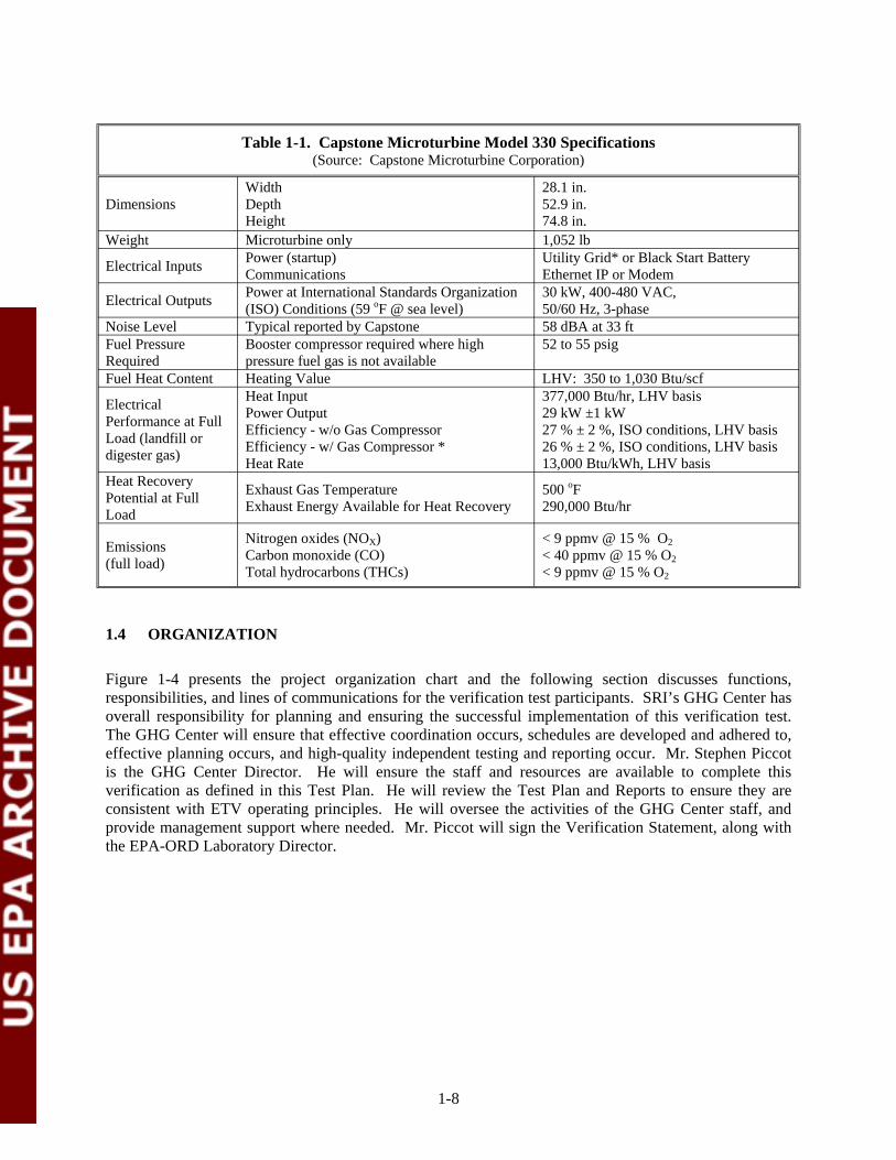
Table 1-1. Capstone Microturbine Model 330 Specifications (Source: Capstone Microturbine Corporation)

Width 28.1 in. Dimensions Depth 52.9 in.

Height 74.8 in. Weight Microturbine only 1,052 lb

Electrical Inputs Power (startup) Communications

Utility Grid* or Black Start Battery Ethernet IP or Modem

Electrical Outputs Power at International Standards Organization (ISO) Conditions (59 oF @ sea level)

30 kW, 400-480 VAC, 50/60 Hz, 3-phase

Noise Level Typical reported by Capstone 58 dBA at 33 ft Fuel Pressure Booster compressor required where high 52 to 55 psig Required pressure fuel gas is not available Fuel Heat Content Heating Value LHV: 350 to 1,030 Btu/scf

Electrical Performance at Full Load (landfill or digester gas)

Heat Input Power Output Efficiency - w/o Gas Compressor Efficiency - w/ Gas Compressor * Heat Rate

377,000 Btu/hr, LHV basis 29 kW ±1 kW 27 % ± 2 %, ISO conditions, LHV basis 26 % ± 2 %, ISO conditions, LHV basis 13,000 Btu/kWh, LHV basis

Heat Recovery Potential at Full Load

Exhaust Gas Temperature Exhaust Energy Available for Heat Recovery

500 oF 290,000 Btu/hr

Emissions (full load)

Nitrogen oxides (NOX) Carbon monoxide (CO) Total hydrocarbons (THCs)

< 9 ppmv @ 15 % O2 < 40 ppmv @ 15 % O2 < 9 ppmv @ 15 % O2

1.4 ORGANIZATION

Figure 1-4 presents the project organization chart and the following section discusses functions, responsibilities, and lines of communications for the verification test participants. SRI’s GHG Center has overall responsibility for planning and ensuring the successful implementation of this verification test. The GHG Center will ensure that effective coordination occurs, schedules are developed and adhered to, effective planning occurs, and high-quality independent testing and reporting occur. Mr. Stephen Piccot is the GHG Center Director. He will ensure the staff and resources are available to complete this verification as defined in this Test Plan. He will review the Test Plan and Reports to ensure they are consistent with ETV operating principles. He will oversee the activities of the GHG Center staff, and provide management support where needed. Mr. Piccot will sign the Verification Statement, along with the EPA-ORD Laboratory Director.

1-8

EPAETV GHG Pilot Manager

EPA - APPCDDavid Kirchgessner

EPAQuality Assurance Manager

EPA - APPCDRobert Wright

Southern Research InstituteQuality Assurance Manager

Ashley Williamson

Southern Research InstituteETV GHG Center Director

Stephen Piccot

Southern Research InstituteETV GHG Center Project Manager

William Chatterton

Southern Research InstituteETV GHG Center Field Team Leader

Robert Richards

Emissions TestingContractor

TRC EnvironmentalCorporation

Analytical LaboratoryEmpact Analytical

Systems, Inc. .

NYSERDAProgram Director

Richard DrakeProject Manager

Joseph Sayer

NYSEGManager of Development

Bruce RolosonProject ManagerJames Harvilla

DDI FARMEManager

Larry Jones

EPA

EPA

.

Proj

Proj

ETV GHG Pilot Manager EPA - APPCD

David Kirchgessner

Quality Assurance Manager EPA - APPCD Robert Wright

Southern Research Institute Quality Assurance Manager

Ashley Williamson

Southern Research Institute ETV GHG Center Director

Stephen Piccot

Southern Research Institute ETV GHG Center Project Manager

William Chatterton

Southern Research Institute ETV GHG Center Field Team Leader

Robert Richards

Emissions Testing Contractor

TRC Environmental Corporation

Analytical Laboratory Empact Analytical

Systems, Inc.

NYSERDA Program Director

Richard Drake ect Manager

Joseph Sayer

NYSEG Manager of Development

Bruce Roloson ect Manager

James Harvilla

DDI FARME Manager

Larry Jones

Figure 1-4. Project Organization

Mr. William Chatterton will serve as the Project Manager. He will be responsible for developing the Test Plan and overseeing field data collection activities of the GHG Center’s Field Team Leader, including assessment of the Team Leader’s accomplishment of DQOs. Mr. Chatterton will ensure the procedures outlined in Sections 2.0 and 3.0 of this Test Plan are adhered to during testing unless modification is required. He is responsible for selecting qualified subcontractors where needed, ensuring their conformance to data quality and safety requirements, and coordinating their activities with the test program. He is also ultimately responsible for conformation that quality control procedures specified in this Test Plan are conducted and criteria met by field personnel and subcontractors. Modifications will be completed, explained, and justified in the Verification Report. Mr. Chatterton will have authority to suspend testing should a situation arise during testing that could affect the health or safety of any personnel. He will also have the authority to suspend testing if quality problems occur or host site or vendor problems arise. He will also be responsible for maintaining effective communications with NYSERDA, DDI, NYSEG, EPA-ORD participants, Southern QA team members, and ETV document reviewers.

Mr. Robert Richards will serve as the Field Team Leader, and will support Mr. Chatterton’s data quality determination activities. Mr. Richards will provide field support for activities related to all measurements and data collected. He will install and operate the measurement instruments, supervise and document activities conducted by the emissions testing contractor, collect gas samples and coordinate sample analysis with the laboratory, and ensure that QA/QC procedures outlined in Section 2.0 are followed. He will submit all results to the Project Manager, such that it can be determined that the DQOs are met. He

1-9

will be responsible for ensuring that performance data collected by continuously monitored instruments and manual sampling techniques are based on procedures described in Section 4.0.

SRI’s Quality Assurance Manager, Dr. Ashley Williamson, will review this Test Plan. He will also review the results from the verification test including all data generated by subcontractors, and conduct an Audit of Data Quality (ADQ), described in Section 4.5. Dr. Williamson will report the results of the internal audits and corrective actions to the GHG Center Director. The results will be used to prepare the final Report.

Mr. Joseph Sayer, Senior Project Manager, will serve as the primary contact person for NYSERDA. Mr. Sayer will provide technical assistance and coordinate operation of the CHP system at the test site. Mr. Sayer will coordinate with the farm operators to ensure the unit and host site are available and accessible to the GHG Center for the duration of the test. NYSERDA’s Manager of Power Systems Research, Mr. Richard Drake, will direct his activities.

Mr. Larry Jones is the operator of the farm. Mr. Bruce Roloson and Mr. Jim Harvilla of NYSEG will design, install, and operate the biogas treatment and the CHP systems. They will conduct preliminary assessment of biogas quality and natural gas blending activities, and will complete the optimization exercises prior to verification testing. DDI and NYSEG will provide access to the test site during verification testing, and ensure safe operation of the system. They will also review the Test Plan and Report, and provide written comments.

EPA-ORD will provide oversight and QA support for this verification. The APPCD Project Officer, Dr. David Kirchgessner, is responsible for obtaining final approval of the Test Plan and Report. The APPCD QA Manager reviews and approves the Test Plan and the final Report to ensure they meet the GHG Center QMP requirements and represent sound scientific practices.

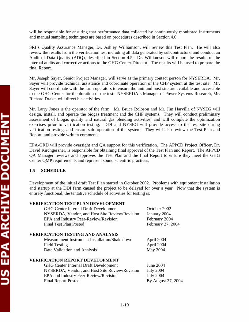
1.5 SCHEDULE

Development of the initial draft Test Plan started in October 2002. Problems with equipment installation and startup at the DDI farm caused the project to be delayed for over a year. Now that the system is entirely functional, the tentative schedule of activities for testing is:

VERIFICATION TEST PLAN DEVELOPMENT GHG Center Internal Draft Development October 2002 NYSERDA, Vendor, and Host Site Review/Revision January 2004EPA and Industry Peer-Review/Revision February 2004

Final Test Plan Posted February 27, 2004

VERIFICATION TESTING AND ANALYSIS Measurement Instrument Installation/Shakedown April 2004 Field Testing April 2004

Data Validation and Analysis May 2004

VERIFICATION REPORT DEVELOPMENT GHG Center Internal Draft Development June 2004 NYSERDA, Vendor, and Host Site Review/Revision July 2004 EPA and Industry Peer-Review/Revision July 2004

Final Report Posted By August 27, 2004

1-10

2.0 VERIFICATION APPROACH

2.1 OVERVIEW OF CHP SYSTEM PERFORMANCE TESTING

CHP systems operating on anaerobic digestion gas are a relatively new application of DG technologies; the availability of performance data in such applications is limited and in great demand. The GHG Center’s stakeholder groups and other organizations concerned with DG have a specific interest in obtaining verified field data on the emissions, technical, and operational performance of DG systems in agricultural applications.

Performance parameters of greatest interest include electrical power output and quality, thermal-to-electrical energy conversion efficiency, thermal energy recovery efficiency, exhaust emissions of conventional air pollutants and GHGs, GHG emission reductions, operational availability, maintenance requirements, and economic performance. The test approach described here focuses on assessing those performance parameters for potential microturbine technology customers. Long-term evaluations cannot be performed with available resources, so economic performance and maintenance requirements will not be evaluated. The ETV verification will evaluate the technical performance of this microturbine CHP system at the conditions encountered during the test period only.

The microturbine CHP system will be evaluated at power outlet levels most likely to be selected by users. Performance testing will be conducted at four electrical loads: 100, 90, 75, and 50 percent of rated power output (30 kW each or 60 kW total, nominal). During each load test, field personnel will simultaneously monitor power output, heat recovery rate, fuel consumption, ambient meteorological conditions, exhaust stack emission rate, and pollutant concentrations. Average electrical power output, heat recovery rate, energy conversion efficiency (electrical, thermal, and net), and exhaust stack concentration and emission rates will be reported for each load factor. The report will also include emission results for the following pollutants for each load condition: CO2, CH4, NOX, CO, sulfur dioxide (SO2), THC, NH3, total particulate matter (TPM), and total reduced sulfur (TRS).

In addition to simulated load testing, the GHG Center will conduct approximately 1-week of extended monitoring to evaluate electrical power quality performance and quantify total electrical and thermal energy produced at normal site operating load conditions. Normal site operating condition is defined as the microturbines running 24-hours per day at maximum electrical power output. Test equipment will monitor power quality parameters such as electrical frequency, voltage output, power factor, and total harmonic distortion (THD) in 1-minute intervals. In addition, continuous logging of power output, fuel input, heat recovery rates, and ambient meteorological conditions, will be performed to quantify total energy produced and to examine daily trends in power and heat production. Emission reductions for CO2 and NOX will be estimated by using the full load emission rates and the electricity offsets from the power grid over the duration of the 1-week test period.

The parameters to be verified are listed below. Detailed descriptions of testing and analytical methods are provided sequentially in Sections 2.2 through 2.5. Section 3.0 discusses data quality assessment procedures for each verification parameter.

2-1

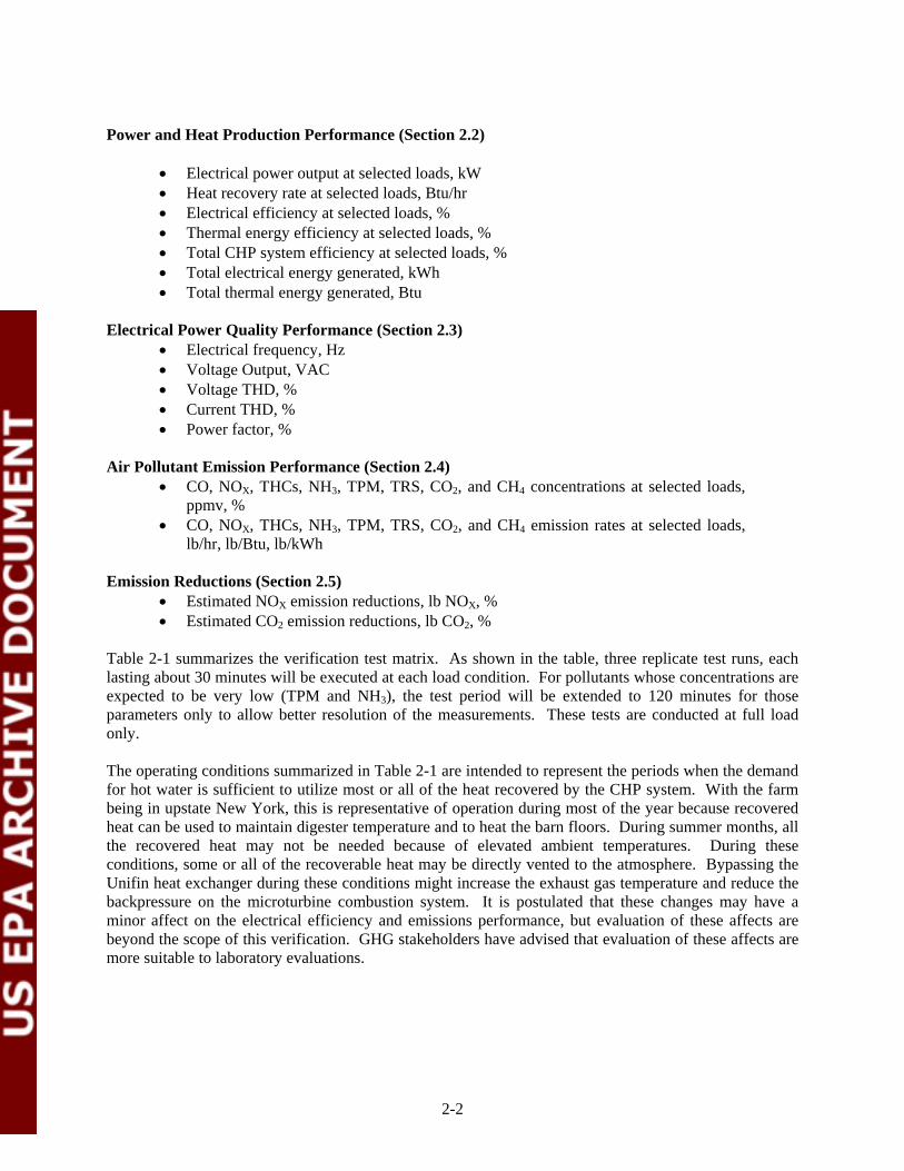
Power and Heat Production Performance (Section 2.2)

• Electrical power output at selected loads, kW • Heat recovery rate at selected loads, Btu/hr • Electrical efficiency at selected loads, % • Thermal energy efficiency at selected loads, % • Total CHP system efficiency at selected loads, % • Total electrical energy generated, kWh • Total thermal energy generated, Btu

Electrical Power Quality Performance (Section 2.3) • Electrical frequency, Hz • Voltage Output, VAC • Voltage THD, % • Current THD, % • Power factor, %

Air Pollutant Emission Performance (Section 2.4) • CO, NOX, THCs, NH3, TPM, TRS, CO2, and CH4 concentrations at selected loads,

ppmv, % • CO, NOX, THCs, NH3, TPM, TRS, CO2, and CH4 emission rates at selected loads,

lb/hr, lb/Btu, lb/kWh

Emission Reductions (Section 2.5) • Estimated NOX emission reductions, lb NOX, % • Estimated CO2 emission reductions, lb CO2, %

Table 2-1 summarizes the verification test matrix. As shown in the table, three replicate test runs, each lasting about 30 minutes will be executed at each load condition. For pollutants whose concentrations are expected to be very low (TPM and NH3), the test period will be extended to 120 minutes for those parameters only to allow better resolution of the measurements. These tests are conducted at full load only.

The operating conditions summarized in Table 2-1 are intended to represent the periods when the demand for hot water is sufficient to utilize most or all of the heat recovered by the CHP system. With the farm being in upstate New York, this is representative of operation during most of the year because recovered heat can be used to maintain digester temperature and to heat the barn floors. During summer months, all the recovered heat may not be needed because of elevated ambient temperatures. During these conditions, some or all of the recoverable heat may be directly vented to the atmosphere. Bypassing the Unifin heat exchanger during these conditions might increase the exhaust gas temperature and reduce the backpressure on the microturbine combustion system. It is postulated that these changes may have a minor affect on the electrical efficiency and emissions performance, but evaluation of these affects are beyond the scope of this verification. GHG stakeholders have advised that evaluation of these affects are more suitable to laboratory evaluations.

2-2

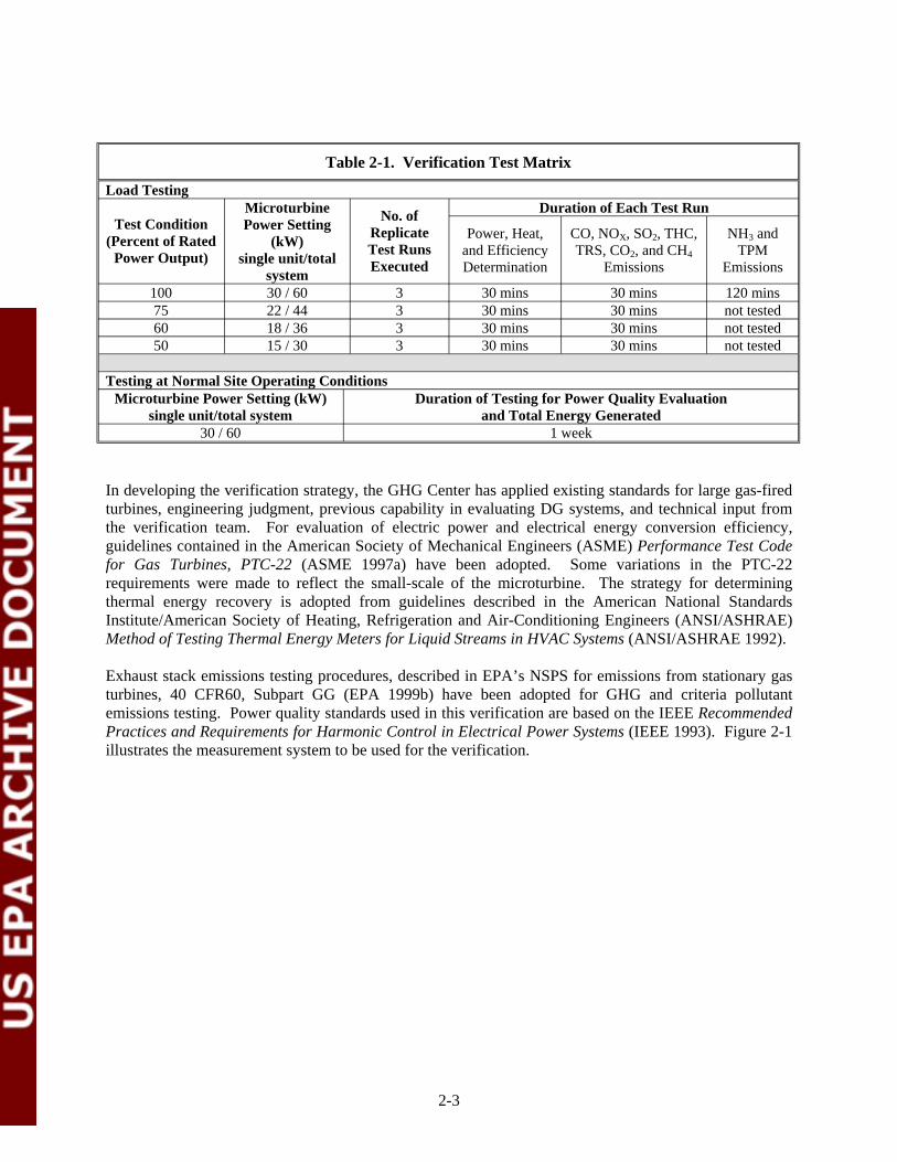
Table 2-1. Verification Test Matrix

Load Testing

Test Condition (Percent of Rated

Power Output)

Microturbine Power Setting

(kW) single unit/total

system

No. of Replicate Test Runs Executed

Duration of Each Test Run

Power, Heat, and Efficiency Determination

CO, NOX, SO2, THC, TRS, CO2, and CH4

Emissions

NH3 and TPM

Emissions

100 30 / 60 3 30 mins 30 mins 120 mins 75 22 / 44 3 30 mins 30 mins not tested 60 18 / 36 3 30 mins 30 mins not tested 50 15 / 30 3 30 mins 30 mins not tested

Testing at Normal Site Operating Conditions Microturbine Power Setting (kW)

single unit/total system Duration of Testing for Power Quality Evaluation

and Total Energy Generated 30 / 60 1 week

In developing the verification strategy, the GHG Center has applied existing standards for large gas-fired turbines, engineering judgment, previous capability in evaluating DG systems, and technical input from the verification team. For evaluation of electric power and electrical energy conversion efficiency, guidelines contained in the American Society of Mechanical Engineers (ASME) Performance Test Code for Gas Turbines, PTC-22 (ASME 1997a) have been adopted. Some variations in the PTC-22 requirements were made to reflect the small-scale of the microturbine. The strategy for determining thermal energy recovery is adopted from guidelines described in the American National Standards Institute/American Society of Heating, Refrigeration and Air-Conditioning Engineers (ANSI/ASHRAE) Method of Testing Thermal Energy Meters for Liquid Streams in HVAC Systems (ANSI/ASHRAE 1992).

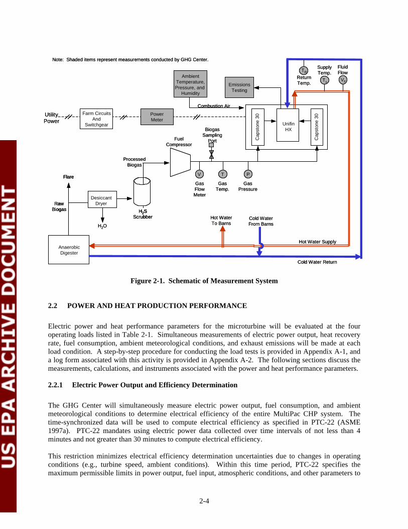
Exhaust stack emissions testing procedures, described in EPA’s NSPS for emissions from stationary gas turbines, 40 CFR60, Subpart GG (EPA 1999b) have been adopted for GHG and criteria pollutant emissions testing. Power quality standards used in this verification are based on the IEEE Recommended Practices and Requirements for Harmonic Control in Electrical Power Systems (IEEE 1993). Figure 2-1 illustrates the measurement system to be used for the verification.

2-3

UnifinHX

Cap

ston

e 30

Cap

ston

e 30

AnaerobicDigester

DesiccantDryer

EmissionsTesting

AmbientTemperature,Pressure, and

Humidity

PowerMeter

Farm CircuitsAnd

Switchgear

Cap

ston

e 30

AnaerobicDigester

DesiccantDryer

Utility Power

Fuel Compressor

Processed Biogas

V

Gas Flow Meter

T

Gas Temp.

P

Gas Pressure

Raw Biogas

Flare

H2S Scrubber

H2O

Combustion Air

VF

Fluid FlowTR

Return Temp. Ts

Supply Temp.

Cold Water Return

Hot Water Supply

Hot Water To Barns

Cold Water From Barns

Biogas Sampling

Port

Note: Shaded items represent measurements conducted by GHG Center.

UtilityPower

FuelCompressor

ProcessedBiogas

V

GasFlowMeter

T

GasTemp.

P

GasPressure

Unifin HX

Cap

ston

e 30

Cap

ston

e 30

RawBiogas

Flare

Anaerobic Digester

RawBiogas

Flare

Desiccant Dryer

H2SScrubber

H2SScrubber

H2O

Emissions Testing

Ambient Temperature, Pressure, and

Humidity

Combustion Air

Power Meter

Farm Circuits And

Switchgear

VF

FluidFlowTR

ReturnTemp. Ts

SupplyTemp.

Cold Water Return

Hot Water Supply

Hot WaterTo Barns

Cold WaterFrom Barns

BiogasSampling

Port

Note: Shaded items represent measurements conducted by GHG Center.

Figure 2-1. Schematic of Measurement System

2.2 POWER AND HEAT PRODUCTION PERFORMANCE

Electric power and heat performance parameters for the microturbine will be evaluated at the four operating loads listed in Table 2-1. Simultaneous measurements of electric power output, heat recovery rate, fuel consumption, ambient meteorological conditions, and exhaust emissions will be made at each load condition. A step-by-step procedure for conducting the load tests is provided in Appendix A-1, and a log form associated with this activity is provided in Appendix A-2. The following sections discuss the measurements, calculations, and instruments associated with the power and heat performance parameters.

2.2.1 Electric Power Output and Efficiency Determination

The GHG Center will simultaneously measure electric power output, fuel consumption, and ambient meteorological conditions to determine electrical efficiency of the entire MultiPac CHP system. The time-synchronized data will be used to compute electrical efficiency as specified in PTC-22 (ASME 1997a). PTC-22 mandates using electric power data collected over time intervals of not less than 4 minutes and not greater than 30 minutes to compute electrical efficiency.

This restriction minimizes electrical efficiency determination uncertainties due to changes in operating conditions (e.g., turbine speed, ambient conditions). Within this time period, PTC-22 specifies the maximum permissible limits in power output, fuel input, atmospheric conditions, and other parameters to

2-4

be less than the values shown in Tables 2-2. The GHG Center will use only those time periods that meet these requirements to compute power and heat performance parameters. Should the variation in any measurement parameter listed in the tables exceed the specified levels, the load test run will be considered invalid and the test run will be repeated.

Table 2-2. Permissible Variations in Power, Fuel, and Atmospheric Conditions

Measured Parameter Maximum Permissible Variation Ambient air temperature ± 4 oF Barometric pressure ± 0.5 % Fuel flow rate ± 2.0 % Power factor ± 2.0 % Power output ± 2.0 %

For each test run, electrical efficiency will be computed as shown in Equation 1. Average electrical efficiency will be the mean of the three test runs.

η14. 3412 kW j

e, j = HI j

100 * (Eqn. 1)

Where: ηe,j = Electrical efficiency at load condition j, % kWj = Average electrical power output at load condition j, kW HIj = Average LHV heat input for load condition j, Btu/hr 3412.14 = Btu/hr per kW

Average electrical power output will be the mathematical average of the 1-minute power output readings measured over the 30 minute test run, and will be computed as shown in Equation 2.

∑ i=nr

kWi

kWj = i =1 (Eqn. 2)nr

Where: KWj = Average electrical power output at load condition j, kW kWi = Average electrical power output during minute i as measured by the power meter, kW nr = Number of 1-minute averages logged during the test run

Heat input, shown in Equation 1, is the average blended gas (fuel) flow rate multiplied by the average fuel LHV. Heat input to the microturbines, normalized to an hourly rate for each test run will be:

HI j = LHVavg , j *Vavg , j (Eqn. 3)

Where: HIj = Heat input at load condition j, Btu/hr LHVavg,j = Average LHV at load condition j, Btu/scf Vavg, j = Average fuel flow rate at load condition j, standard cubic feet per hour (scfh)

2-5

Electrical power output measurements will be performed with a 7600 ION watt meter. The meter will be installed at the outlet of the MultiPac CHP system, and will represent actual net power delivered to the site for consumption, as reduced by the parasitic loads (Figure 2-1). It will not include power used by the booster compressor and other parasitic losses outside of the CHP system. Section 2.2.3.1 describes the power meter to be used.

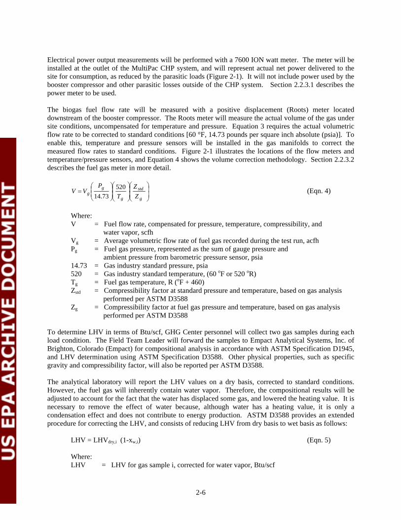
The biogas fuel flow rate will be measured with a positive displacement (Roots) meter located downstream of the booster compressor. The Roots meter will measure the actual volume of the gas under site conditions, uncompensated for temperature and pressure. Equation 3 requires the actual volumetric flow rate to be corrected to standard conditions [60 °F, 14.73 pounds per square inch absolute (psia)]. To enable this, temperature and pressure sensors will be installed in the gas manifolds to correct the measured flow rates to standard conditions. Figure 2-1 illustrates the locations of the flow meters and temperature/pressure sensors, and Equation 4 shows the volume correction methodology. Section 2.2.3.2 describes the fuel gas meter in more detail.

Pg

73.14

⎛ ⎛⎞ ⎞⎛ ⎞ Z520⎜⎜⎝ ⎟⎟⎠

⎜⎜⎝ ⎟⎟⎠

std

Z ⎟⎟⎠

⎜⎜⎝

(Eqn. 4)V =Vg Tg g

Where: V = Fuel flow rate, compensated for pressure, temperature, compressibility, and

water vapor, scfh Vg = Average volumetric flow rate of fuel gas recorded during the test run, acfh Pg = Fuel gas pressure, represented as the sum of gauge pressure and

ambient pressure from barometric pressure sensor, psia 14.73 = Gas industry standard pressure, psia 520 = Gas industry standard temperature, (60 oF or 520 oR) Tg = Fuel gas temperature, R (oF + 460) Zstd = Compressibility factor at standard pressure and temperature, based on gas analysis

performed per ASTM D3588 Zg = Compressibility factor at fuel gas pressure and temperature, based on gas analysis

performed per ASTM D3588

To determine LHV in terms of Btu/scf, GHG Center personnel will collect two gas samples during each load condition. The Field Team Leader will forward the samples to Empact Analytical Systems, Inc. of Brighton, Colorado (Empact) for compositional analysis in accordance with ASTM Specification D1945, and LHV determination using ASTM Specification D3588. Other physical properties, such as specific gravity and compressibility factor, will also be reported per ASTM D3588.

The analytical laboratory will report the LHV values on a dry basis, corrected to standard conditions. However, the fuel gas will inherently contain water vapor. Therefore, the compositional results will be adjusted to account for the fact that the water has displaced some gas, and lowered the heating value. It is necessary to remove the effect of water because, although water has a heating value, it is only a condensation effect and does not contribute to energy production. ASTM D3588 provides an extended procedure for correcting the LHV, and consists of reducing LHV from dry basis to wet basis as follows:

LHV = LHVdry,i (1-xw,i) (Eqn. 5)

Where: LHV = LHV for gas sample i, corrected for water vapor, Btu/scf

2-6

LHVdry,I = LHV for gas sample i, reported on dry basis by analytical laboratory, Btu/scf xw,i = mole fraction of water in gas sample i

The term “xw” is the mole fraction of water vapor in the gas stream. To account for fuel moisture, and its effects on LHV, GHG Center personnel will determine fuel gas moisture content in the field by ASTM D4888-88 “Standard Test Method for Water Vapor in Natural Gas Using Length-of-Stain Detector Tubes” (ASTM 1999). Appendix A-5 provides the procedure and log form.

Section 2.2.3.4 describes the fuel gas sampling and analysis procedures.

2.2.2 Heat Recovery Rate and Thermal Efficiency Determination

The CHP system produces heat as a byproduct of electricity generation. The amount of heat recovered is a function of the recovery potential of the CHP system and the thermal energy demand of the site. At the host site, the recovered heat is transferred to a circulating hot water system, which is routed to the digester to maintain a constant operating temperature. Excess heat is used for space heating purposes. Unused heat is automatically expelled through the CHP system exhaust stack.

The primary purpose of the heat recovery loop is to maintain digester temperature at about 100 °F. Depending on the thermal demand of the digester and ambient temperatures, cool water returning from the digester is expected to range between 105 and 125 oF. Since the primary goal of the load testing is to characterize maximum heat recovery potential of the system, engineering calculations suggest that a temperature differential of about 15 oF is required to recover the remaining 74 percent [558 thousand British thermal units per hour (Btu/hr) at full load] of the heat input remaining after electrical power generation. This equates to hot water (supply) temperatures ranging between 120 and 140 oF. The CHP system will be set to recover maximum heat by pre-setting the hot water supply temperatures to these levels. Table 2-3 summarizes the target temperature differentials as a function of load levels and return temperatures. The heat recovery rate, measured at full load, will represent maximum heat recovery potential of the microturbine CHP system.

Table 2-3. Target Set-Points for Heat Recovery Unit Test Condition Estimated Fuel Estimated Electrical Estimated Heat Available Estimated

(Percent of Rated Input Efficiency, ISO Conditions for Recovery Differential Power Output) (MBtu/hr) (%) (MBtu/hr) Temperature (oF)

100 754 26 558 15

90 714 25.8 530 13

75 628 25 471 12

50 445 23 343 8

Since verification testing is planned to occur in early spring, ambient temperatures are likely to be relatively low. As such, it is expected that most of the heat recovered by the CHP systems will be consumed on-site, and little to no energy will be discarded through the exhaust stack. Heat recovery rates will be computed according to ANSI/ASHRAE Standard 125 (ASHRAE 1992), as follows:

2-7

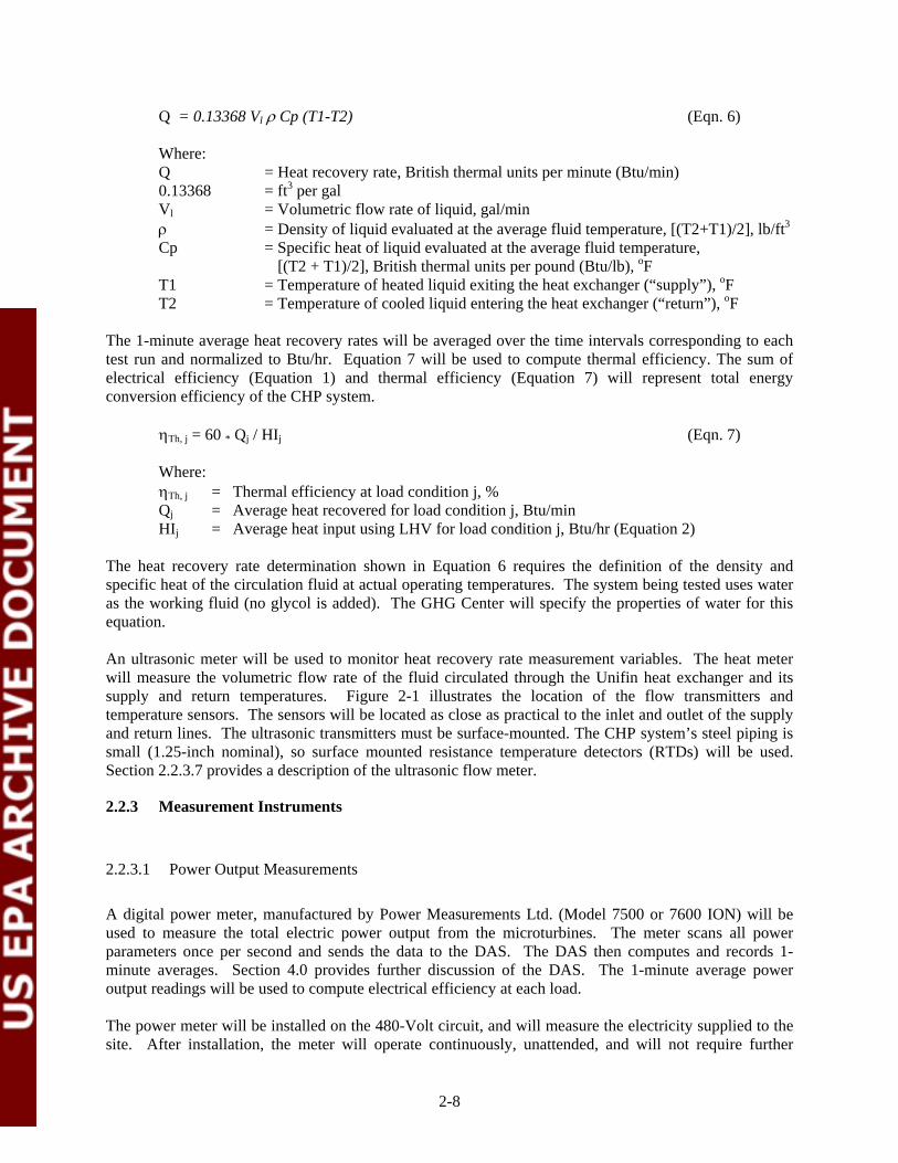
Q = 0.13368 Vl ρ Cp (T1-T2) (Eqn. 6)

Where: Q = Heat recovery rate, British thermal units per minute (Btu/min) 0.13368 = ft3 per gal Vl = Volumetric flow rate of liquid, gal/min ρ = Density of liquid evaluated at the average fluid temperature, [(T2+T1)/2], lb/ft3

Cp = Specific heat of liquid evaluated at the average fluid temperature, [(T2 + T1)/2], British thermal units per pound (Btu/lb), oF

T1 = Temperature of heated liquid exiting the heat exchanger (“supply”), oF T2 = Temperature of cooled liquid entering the heat exchanger (“return”), oF

The 1-minute average heat recovery rates will be averaged over the time intervals corresponding to each test run and normalized to Btu/hr. Equation 7 will be used to compute thermal efficiency. The sum of electrical efficiency (Equation 1) and thermal efficiency (Equation 7) will represent total energy conversion efficiency of the CHP system.

ηTh, j = 60 * Qj / HIj (Eqn. 7)

Where: ηTh, j = Thermal efficiency at load condition j, % Qj = Average heat recovered for load condition j, Btu/min HIj = Average heat input using LHV for load condition j, Btu/hr (Equation 2)

The heat recovery rate determination shown in Equation 6 requires the definition of the density and specific heat of the circulation fluid at actual operating temperatures. The system being tested uses water as the working fluid (no glycol is added). The GHG Center will specify the properties of water for this equation.

An ultrasonic meter will be used to monitor heat recovery rate measurement variables. The heat meter will measure the volumetric flow rate of the fluid circulated through the Unifin heat exchanger and its supply and return temperatures. Figure 2-1 illustrates the location of the flow transmitters and temperature sensors. The sensors will be located as close as practical to the inlet and outlet of the supply and return lines. The ultrasonic transmitters must be surface-mounted. The CHP system’s steel piping is small (1.25-inch nominal), so surface mounted resistance temperature detectors (RTDs) will be used. Section 2.2.3.7 provides a description of the ultrasonic flow meter.

2.2.3 Measurement Instruments

2.2.3.1 Power Output Measurements

A digital power meter, manufactured by Power Measurements Ltd. (Model 7500 or 7600 ION) will be used to measure the total electric power output from the microturbines. The meter scans all power parameters once per second and sends the data to the DAS. The DAS then computes and records 1­minute averages. Section 4.0 provides further discussion of the DAS. The 1-minute average power output readings will be used to compute electrical efficiency at each load.

The power meter will be installed on the 480-Volt circuit, and will measure the electricity supplied to the site. After installation, the meter will operate continuously, unattended, and will not require further

2-8

adjustments. Prior to use in the field, the meter will be factory calibrated to IEC687 SO.2 and ANSI C12.20 CAO.2 standards for accuracy. The accuracy of the power meter and associated current transformers is ± 1.0 percent. Details regarding this and additional QA/QC checks (instrument setup, calibration, and sensor function checks) on this instrument are provided in Section 3.2.

2.2.3.2 Gas Flow Meter

A gas meter is used to measure biogas flow rates to the microturbines. For efficiency determination, the average fuel gas flow rate, multiplied by the average fuel gas LHV, yields average heat input to the CHP system (Equation 3). The meter is a Roots (Model 3M175 SSM, Series B3) rotary positive displacement meters manufactured by DMD-Dresser. The meters’ rated capacities is 3,000 actual cubic feet per hour (acfh), or approximately 50 cubic feet per minute (cfm). This capacity is appropriate for the microturbine’s expected demand of 4 to 15 scfm. Certified accuracy of the meter is ± 1.0 percent of reading.

The gas meter has a totalizing counter, or “index”, which shows the running total of the gas volume that has passed through the meter. The GHG Center will equip the gas meter with a Roots CEX electronic transmitter that provides a non-compensated, high frequency pulse output. The Roots transmitter will produce electronic pulses at a rate of approximately 1,100 to 4,800 pulses per minute. The meter will also be equipped with a pulse input totalizer/ratemeter (Roots Model DM-2 or equivalent) that converts the transmitted pulse signals to a continuous 4 - 20 mA analog output. Using the GHG Center's DAS, the analog output signals will be scaled over the operating range of the meters, continuously logged, and compiled as 1-minute averages.

2.2.3.3 Gas Temperature and Pressure Measurements

Gas temperature will be monitored using an Omega Model 93-K2 Type K thermocouple and transmitter. The sensor will be installed in a thermowell in the biogas fuel line downstream of the flow meter (Figure 2-1). The DAS will record 1-minute average gas temperatures as transmitted by the 4-20 mA signal transmitter. GHG Center analysts will compute the average fuel gas temperature for each test run and the resulting value (oF + 460) will be used as the “Tg” term in Equation 5. The sensor’s range is from 0 to 200 oF, and accuracy is ± 1.5 percent of reading. The thermocouple will be calibrated against a NIST traceable standard across its range.

Fuel gas pressure will be monitored using an Omegas Model PX205-030AI or equivalent. The transducer has a range of 0 to 30 psia and a rated accuracy of ± 0.3 percent of full-scale. The transducer will monitor gas pressure on the upstream side of the gas flow meter (Figure 2-1). The DAS will record 1-minute averages and the Field Team Leader will enter the average fuel gas pressure for each test run as “Pg” in Equation 5. The transducer will be calibrated against a NIST traceable standard across its range.

2.2.3.4 Gas Composition and Heating Value Analysis

The Field Team Leader will collect biogas samples and submit them to Empact to obtain the LHV data required by Equation 3 and the compressibility data required by Equation 4. Test personnel will collect at least two samples spaced throughout each short-term load testing condition. At least two additional samples will be collected at both the beginning and end of the extended monitoring period. Samples will be collected downstream of the gas treatment system to ensure that gas composition is representative of the CHP system fuel (i.e., moisture and H2S removed from raw biogas) for the efficiency determinations.

2-9

A tee fitting and ball valve located in the fuel pipeline between the gas metering equipment and the CHP will provide access for the 600-ml stainless-steel gas sampling canisters. The laboratory evacuates the canisters to prepare them for sampling. Test personnel will check the canisters with a vacuum gauge to ensure that they remain under vacuum and are leak-free prior to sample collection. Canisters that are not fully evacuated will not be used or will be evacuated on site and checked again before use. Appendices A-3, A-4, and A-6 contain detailed sampling procedures, log, and chain-of-custody forms.

The Field Team Leader will submit the collected samples to Empact for compositional analysis. All samples shipped to the laboratory will be accompanied by appropriate chain-of-custody forms and documentation of sample identification, matrix, date and time of collection, analyses required, methods and release signature. Analyses will be in accordance with ASTM Specification D1945 for quantification of speciated hydrocarbons including methane through pentane (C1 through pentane C5), heavier hydrocarbons (grouped as hexanes plus C6+), N2, O2, and CO2. The lab procedure specifies sample gas is injected into a Hewlett Packard 589011 gas chromatograph equipped with a molecular sieve column and a thermal conductivity detector (TCD). The column physically separates gas components, the TCD detects them, and the instrument plots the chart traces and calculates the resultant areas for each compound. The instrument then compares these areas to the areas of the same compounds contained in a calibration reference standard analyzed under identical conditions. The reference standard areas are used to determine instrument response factors for each compound and these factors are used to calculate the component concentrations in the sample.

The laboratory calibrates the instruments weekly with the reference standards. The instrument operator programs the analytical response factors generated for each compound analyzed into the instrument during calibrations. Allowable method error during calibration is ± 1 percent of the reference value of each gas component. The laboratory re-calibrates the instrument whenever its performance is outside the acceptable calibration limit of ± 1 percent for each component. The GHG Center will obtain and review the calibration records.

In addition to the ASTM D1945 compositional analyses, Gas Processors Association (GPA) Method 2286 will provide an extended analysis to quantify concentrations of H2S (GPA 2000). GPA Method 2286 is essentially an extension of the ASTM D1945 procedures that uses additional chromatographic columns to separate H2S and heavier hydrocarbons. After injection into the GC, the sample is split. The first column separates and detects oxygen, nitrogen, H2S, and CH4 using the thermal conductivity detector referenced above. The second column separates ethane through normal pentane and employs a FID. The third section, not needed for this testing, separates and quantifies iso-pentane through tetradecane using a third column and a second FID. Consistent with the calibration procedures specified in ASTM D1945, analytical response factors for each compound are established by analyzing a calibration reference standard under identical conditions.

2.2.3.5 Fuel Moisture Analysis

GHG Center personnel will determine fuel gas moisture content in the field by ASTM D4888-88 (ASTM 1999). In this test, a calibrated hand pump (Drager 18350 or equivalent) passes the gas through a detector tube (Drager 26228 or equivalent) filled with a specially prepared chemical. Any water vapor present in the sample reacts with the chemical to produce a color change or stain. The length of the stain, when exposed to a measured volume of gas, is directly proportional to the amount of water vapor in the gas. The test operator compares the length of the stain to the manufacturer’s calibration scale to yield water vapor content in milligram per liter (mg/l). The analytical range is selectable based on anticipated vapor levels. Accuracy of the ASTM procedure is approximately 25 percent of reading, and the tubes are sensitive to 1 mg/l of H2O.

2-10

The Field Team Leader will acquire at least one moisture sample in conjunction with each fuel gas sample for a total of two per load. As a check for the method’s repeatability, he will acquire back-to-back moisture samples at least twice per day during load tests. Each back-to-back sample will be collected immediately after the preceding moisture sample. Logged values should agree with each other within 25 percent. Appendix A-5 provides the log form.

2.2.3.6 Ambient Conditions Measurements

The ambient meteorological conditions (temperature, relative humidity, and barometric pressure) will be monitored using a pressure sensor and an integrated temperature/humidity unit located in close proximity to the air intake of the microturbines. A Vaisala Model HMD 60YO will be used. The integrated temperature/humidity unit uses a platinum RTD for temperature measurement. As the temperature changes, the resistance of the RTD changes. This resistance change is detected and converted by associated electronic circuitry that provides a linear (DC 4-20mA) output signal. A thin film capacitive sensor measures humidity. The dielectric polymer capacitive element varies in capacitance as the relative humidity varies. Internal electronics convert the capacitance change into a linear output signal (DC 4-20 mA).

A Setra Model 280E ambient pressure sensor will be used to monitor barometric pressure (psia). This instrument also employs a variable capacitance sensor. The capacitance decreases as pressure increases; full-scale span is 25.0 psia. Accuracy is ± 0.1 percent of full scale. The GHG Center’s DAS will convert the 0-5 volt analog signals to digital format and then store the data as 1-minute averages. Each sensor will be calibrated to NIST-traceable standards.

2.2.3.7 Heat Recovery Rate Measurements

The GHG Center will use a portable Controlotron (Model 1010EPTRE) heat meter to quantify the heat recovery rate. The heat meter is a digitally integrated system which consists of a portable computer, ultrasonic fluid flow transmitters, and 1,000 ohm platinum RTDs. The fluid velocity measured by the ultrasonic transmitters is converted to liquid flow rate using pipe dimensions and other physical properties (e.g., pipe diameter, pipe wall thickness). The RTDs measure the supply and return side temperatures. The heat meter provides the following analog outputs:

Measurement Units Fluid flow rate gal/min Return temperature oF Supply temperature oF

During all test periods, the GHG Center’s DAS will log the heat meter outputs as 1-minute averages.

The heat meter can be can be used on pipe sizes ranging from 0.25 to 360 inches in diameter, with fluid flow rates ranging from 0 to 60 feet per second. The flow transducers are external surface mounted units. They are rated a sensitivity of 0.001 feet per second with repeatability of 0.25 percent. The flow computer measures the transit time of the ultrasonic pulses and converts it to fluid velocity. It then multiplies the fluid velocity by the internal area of the pipe to yield volumetric flow rate.

The test operator mounts the ultrasonic transducers on the pipe at least ten diameters from upstream and five diameters from the downstream disturbances (e.g., elbows, valves.). The accuracy of the flow meter is ± 1.5 percent of reading. The RTDs are mounted as close to the heat recovery unit as configuration

2-11

allows. They provide continuous supply and return fluid line temperatures to the computer, which calculates the temperature difference. The RTDs have a rated differential temperature accuracy of ± 0.02 oF. The overall rated accuracy of the heat recovery rate is less than ± 2 percent of reading.

Several QA/QC procedures will be conducted prior to and during the verification testing to evaluate the accuracy of the meter. These procedures, which include factory calibration of sensors and independent performance checks in the field, are detailed in Section 3.3.5.

2.3 POWER QUALITY PERFORMANCE

When an electrical generator is connected in parallel and operated simultaneously with the utility grid, there are a number of issues of concern. The voltage and frequency generated by the power system must be aligned with the power grid. While in grid parallel mode, the units must detect grid voltage and frequency to ensure proper synchronization before actual grid connection occurs. The microturbines at the DDI farm accomplish this by converting high-frequency electrical output or adjusting rpm to match the grid frequency and voltage. The microturbine power electronics contain circuitry to detect and react to abnormal conditions that, if exceeded, cause the unit to automatically disconnect from the grid. These out-of-tolerance operating conditions include overvoltages, undervoltages, and over/under frequency. For previous verifications, the GHG Center has defined grid voltage tolerance as the nominal voltage ± 10 percent. Frequency tolerance is 60 ± 0.6 Hz (1.0 percent).

The power factor delivered by each system must be close to unity (100 percent) to avoid billing surcharges. Harmonic distortions in voltage and current must also be minimized to reduce damage or disruption to electrical equipment (e.g., lights, motors, office equipment). Industry standards for harmonic distortion have been established within which power generation equipment must operate.

The generator’s effects on electrical frequency, power factor, and THD cannot be completely isolated from the grid. The quality of power delivered actually represents an aggregate of disturbances already present in the utility grid. For example, local CHP power with low THD will tend to dampen grid power with high THD in the test facility’s wiring network. This effect will drop off with distance from the CHP generator.

Synchronous generators usually operate at or near unity (100 percent) power factor. Induction generators, however, always require reactive power from the grid and operate at less than unity power factor. In either case, the generator’s power factor effects will also change with distance from the CHP generator as the aggregate grid power factor begins to predominate.

The GHG Center and its stakeholders developed the following power quality evaluation approach to account for these issues. Two documents (IEEE 1993, ANSI/IEEE 1989) form the basis for selecting the power quality parameters of interest and the measurement methods to be used. The GHG Center will measure and record the following power quality parameters for seven (7) days of operation at normal site conditions:

• Electrical frequency • Voltage • Voltage THD • Current THD • Power factor

2-12

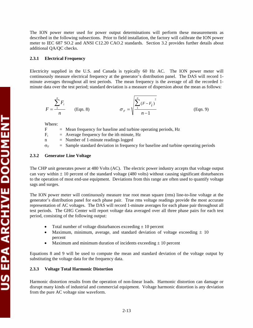
The ION power meter used for power output determinations will perform these measurements as described in the following subsections. Prior to field installation, the factory will calibrate the ION power meter to IEC 687 SO.2 and ANSI C12.20 CAO.2 standards. Section 3.2 provides further details about additional QA/QC checks.

2.3.1 Electrical Frequency

Electricity supplied in the U.S. and Canada is typically 60 Hz AC. The ION power meter will continuously measure electrical frequency at the generator’s distribution panel. The DAS will record 1­minute averages throughout all test periods. The mean frequency is the average of all the recorded 1­minute data over the test period; standard deviation is a measure of dispersion about the mean as follows:

n n

∑ Fi ∑ (F − Fi )2

1 1F = (Eqn. 8) σ F = (Eqn. 9) n n −1

Where: F = Mean frequency for baseline and turbine operating periods, Hz Fi = Average frequency for the ith minute, Hz n = Number of 1-minute readings logged σF = Sample standard deviation in frequency for baseline and turbine operating periods

2.3.2 Generator Line Voltage

The CHP unit generates power at 480 Volts (AC). The electric power industry accepts that voltage output can vary within ± 10 percent of the standard voltage (480 volts) without causing significant disturbances to the operation of most end-use equipment. Deviations from this range are often used to quantify voltage sags and surges.

The ION power meter will continuously measure true root mean square (rms) line-to-line voltage at the generator’s distribution panel for each phase pair. True rms voltage readings provide the most accurate representation of AC voltages. The DAS will record 1-minute averages for each phase pair throughout all test periods. The GHG Center will report voltage data averaged over all three phase pairs for each test period, consisting of the following output:

• Total number of voltage disturbances exceeding ± 10 percent • Maximum, minimum, average, and standard deviation of voltage exceeding ± 10

percent • Maximum and minimum duration of incidents exceeding ± 10 percent

Equations 8 and 9 will be used to compute the mean and standard deviation of the voltage output by substituting the voltage data for the frequency data.

2.3.3 Voltage Total Harmonic Distortion

Harmonic distortion results from the operation of non-linear loads. Harmonic distortion can damage or disrupt many kinds of industrial and commercial equipment. Voltage harmonic distortion is any deviation from the pure AC voltage sine waveform.

2-13

The ION power meter applies Fourier analysis algorithms to quantify THD. Fourier showed that any wave form can be analyzed as one sum of pure sine waves with different frequencies. He also showed that each contributing sine wave is an integer multiple (or harmonic) or the lowest (or fundamental) frequency. For electrical power in the US, the fundamental is 60 Hz. The 2nd harmonic is 120 Hz, the 3rd

is 180 Hz, and so on. Certain harmonics, such as the 5th or 12th, can be strongly affected by the types of devices (i.e. capacitors, motor control thyristors, inverters) connected to the distribution network.

For each harmonic, the magnitude of the distortion can vary. Typically, each harmonic’s magnitude is represented as a percentage of the rms voltage of the fundamental. The aggregate effect of all harmonics is called THD. THD amounts to the sum of the rms voltage of all harmonics divided by the rms voltage of the fundamental, converted to a percentage. THD gives a useful summary view of the generator’s overall voltage quality.

Based on “recommended practices for individual customers” in the IEEE 519 Standard (IEEE 1992), the specified value for total voltage harmonic is a maximum THD of 5.0 percent. The ION meter will continuously measure voltage THD up to the 63rd harmonic for each phase. The meter’s output value is the result of the following calculation:

63⎡ ⎤∑volti⎢⎢⎢⎢⎣

⎥⎥⎥⎥⎦

2THDvolt = 100 * (Eqn. 10) volt1

Where: THDvolt = Voltage THD, % volti = rms voltage reading for the ith harmonic, volts volt1 = rms voltage reading for the fundamental, volts (220, 480, etc.)

The DAS will record 1-minute voltage THD averages for each phase throughout all test periods. The GHG Center will report periods for which overall voltage THD exceeded 5.0 percent, mean, and standard deviation averaged over all three phases for each test period, per the methods outlined in equations 8 and 9 above.

2.3.4 Current Total Harmonic Distortion

Current THD is any distortion of the pure current AC sine waveform and, similar to voltage THD, can be quantified by Fourier analysis. The current THD limits recommended in the IEEE 519 Standard (IEEE 1992) range from 5.0 percent to 20.0 percent, depending on the size of the CHP generator, the test facility’s demand, and its distribution network design as compared to the capacity of the local utility grid. For example, the standard’s recommendations for a small CHP unit connected to a large capacity grid are more forgiving than those for a large CHP unit connected to a small capacity grid.

Detailed analysis of the facility’s distribution network and the local grid are beyond the scope of this verification. The GHG Center will, therefore, report current THD data without reference to a particular recommendation. As with voltage THD, the ION power meter will continuously measure current THD for each phase. The DAS will record 1-minute current THD averages for each phase throughout all test periods. The GHG Center will report mean, and standard deviation of current THD averaged over all three phases for each test period, per the methods outlined in Equations 8 and 9 above.

2-14

2.3.5 Power Factor

Power factor is the phase relationship of current and voltage in AC electrical distribution systems. Under ideal conditions, current and voltage are in phase, which results in a unity (100 percent) power factor. If reactive loads are present, power factors are less than this optimum value. Although it is desirable to maintain unity power factor, the actual power factor of the electricity supplied by the utility may be much lower because of load demands of different end users. Typical values ranging between 70 and 90 percent are common. Low power factor causes heavier current to flow in power distribution lines for a given number of real kilowatts delivered to an electrical load.

The ION power meter will continuously measure average power factor across each generator phase. The DAS will record one-minute averages for each phase during all test periods. The GHG Center will report maximum, minimum, mean, and standard deviation averaged over all three phases per the methods outlined in Equations 8 and 9 above.

2.3.6 Power Quality Measurement Instruments

The ION power meter is capable of measuring all power quality parameters. One-minute average measurement data will be recorded in the DAS. Prior to installation in the field, the meter will be factory calibrated to IEC687 SO.2 and ANSI C12.20 CAO.2 standards for accuracy. Details regarding this and additional QA/QC checks (instrument setup, calibration, sensor function checks) on this instrument are provided in Section 3.2.

2.4 EMISSIONS PERFORMANCE

2.4.1 Stack Emission Rate Determination

Exhaust stack emissions testing will be conducted on the CHP system to determine emission rates for criteria and other pollutants (CO, NOX, NH3, SO2, THCs, and TRS), greenhouse gases (CH4 and CO2), and TPM. Sampling for particulate matter will include quantification of TPM only because the small exhaust stack precludes sampling for PM2.5 and PM10. The sampling apparatus needed to quantify these parameters is too large to fit into this duct. Using the test procedures presented here, the reported particulate emission rate (TPM) will consist of the sum of emissions of PM2.5, PM10, and particles larger than PM10.

As discussed earlier, the stack emission measurements will be conducted simultaneously with efficiency measurements. Following NSPS guidelines for evaluation of emissions from stationary gas turbines, exhaust stack emissions testing will be conducted at four loads within the normal operating range of the microturbine. The test matrix was presented earlier in Table 2-1, and will include testing at 50, 75, 90, and 100 percent of the normal full load capacity.

Note that emissions testing for TPM and NH3 will be conducted only at the highest load factor. Because of relatively low concentrations expected for these two pollutants, the test duration will be extended to 120 minutes. All three full load test replicates for efficiency and gaseous pollutant (each 30 minutes in duration) will be conducted during the first TPM/NH3 test run. The remaining two TPM/NH3 test runs will then be conducted by allowing the system to generate electricity at full load for 4 additional hours. Testing at 90, 75, and 50 percent of rated power output will follow after all pollutant measurements are completed.

2-15

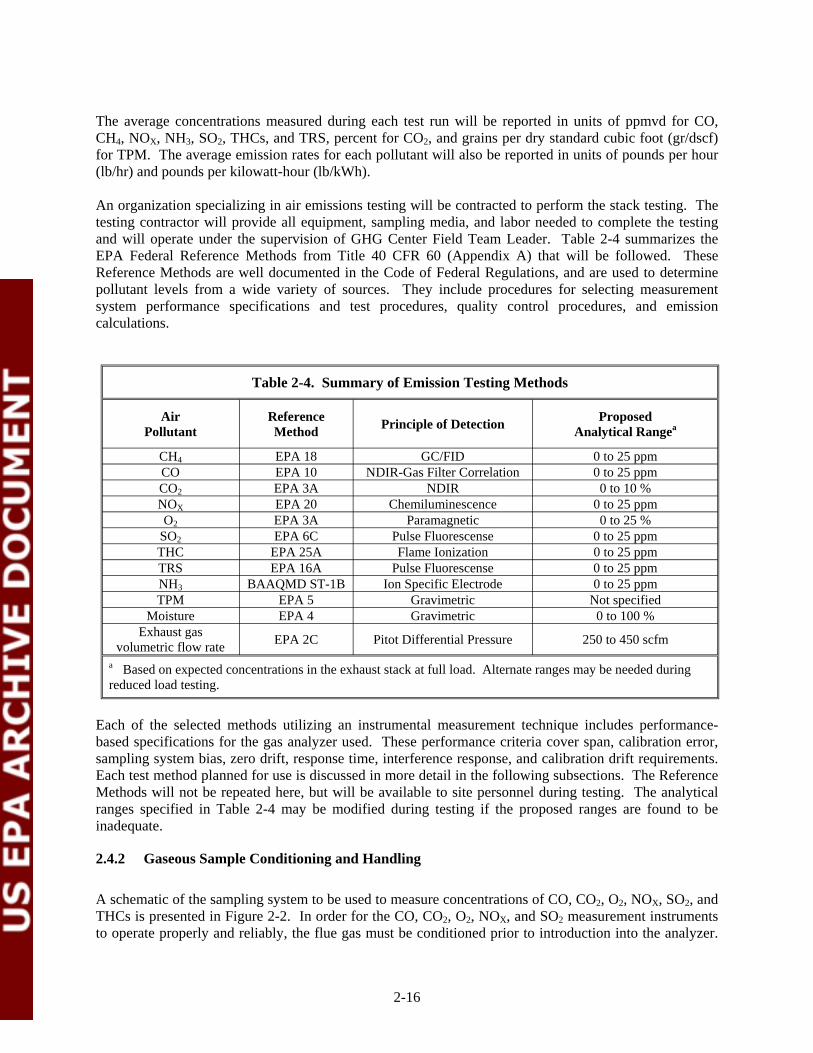
The average concentrations measured during each test run will be reported in units of ppmvd for CO, CH4, NOX, NH3, SO2, THCs, and TRS, percent for CO2, and grains per dry standard cubic foot (gr/dscf) for TPM. The average emission rates for each pollutant will also be reported in units of pounds per hour (lb/hr) and pounds per kilowatt-hour (lb/kWh).

An organization specializing in air emissions testing will be contracted to perform the stack testing. The testing contractor will provide all equipment, sampling media, and labor needed to complete the testing and will operate under the supervision of GHG Center Field Team Leader. Table 2-4 summarizes the EPA Federal Reference Methods from Title 40 CFR 60 (Appendix A) that will be followed. These Reference Methods are well documented in the Code of Federal Regulations, and are used to determine pollutant levels from a wide variety of sources. They include procedures for selecting measurement system performance specifications and test procedures, quality control procedures, and emission calculations.

Table 2-4. Summary of Emission Testing Methods

Air Pollutant

Reference Method Principle of Detection Proposed

Analytical Rangea

CH4 EPA 18 GC/FID 0 to 25 ppm CO EPA 10 NDIR-Gas Filter Correlation 0 to 25 ppm CO2 EPA 3A NDIR 0 to 10 % NOX EPA 20 Chemiluminescence 0 to 25 ppm O2 EPA 3A Paramagnetic 0 to 25 %

SO2 EPA 6C Pulse Fluorescense 0 to 25 ppm THC EPA 25A Flame Ionization 0 to 25 ppm TRS EPA 16A Pulse Fluorescense 0 to 25 ppm NH3 BAAQMD ST-1B Ion Specific Electrode 0 to 25 ppm TPM EPA 5 Gravimetric Not specified

Moisture EPA 4 Gravimetric 0 to 100 % Exhaust gas

volumetric flow rate EPA 2C Pitot Differential Pressure 250 to 450 scfm

a Based on expected concentrations in the exhaust stack at full load. Alternate ranges may be needed during reduced load testing.

Each of the selected methods utilizing an instrumental measurement technique includes performance­based specifications for the gas analyzer used. These performance criteria cover span, calibration error, sampling system bias, zero drift, response time, interference response, and calibration drift requirements. Each test method planned for use is discussed in more detail in the following subsections. The Reference Methods will not be repeated here, but will be available to site personnel during testing. The analytical ranges specified in Table 2-4 may be modified during testing if the proposed ranges are found to be inadequate.

2.4.2 Gaseous Sample Conditioning and Handling

A schematic of the sampling system to be used to measure concentrations of CO, CO2, O2, NOX, SO2, and THCs is presented in Figure 2-2. In order for the CO, CO2, O2, NOX, and SO2 measurement instruments to operate properly and reliably, the flue gas must be conditioned prior to introduction into the analyzer.

2-16

The gas conditioning system is designed to remove water vapor from the sample. All interior surfaces of the gas conditioning system are made of stainless steel, Teflon™, or glass to avoid or minimize any reactions with the sample gas components.

Gas is extracted from the exhaust duct through a stainless steel probe and sample line. The gas is then transported using a sample pump to a gas conditioning system that removes moisture. The clean, dry sample is then transported to a flow distribution manifold where sample flow to each analyzer is controlled. Calibration gases can be routed through this manifold to the sample probe by way of a Teflon line. This allows calibration and bias checks to include all components of the sampling system. The distribution manifold also routes calibration gases directly to the analyzers, where linearity checks are made on each.

The THC analyzer is equipped with a FID. This detector analyzes gases on a wet, unconditioned basis. Therefore, a second, heated sample line is used to deliver unconditioned exhaust gases from the probe to the THC analyzer.

THC

CO2

CO

O2

SO2

Moisture Removal System

Condensate

Heated Sampling Probe

System Calibration Gas Sample and Calibration Gas Control Manifold

Calibration Gases

Sampling Pump

System Exhaust

Analyzer

NOx Analyzer

Analyzer

Analyzer

Analyzer

Data Acquisition

System

Heated Sample Lines

Unheated Sample Lines

Analyzer

3-way Valve

Figure 2-2. Gaseous Pollutant Sampling System

2.4.3 Gaseous Pollutant Sampling Procedures

This section provides a brief description of the sampling procedures and instrumentation needed to determine concentrations of each of the gaseous pollutants. QA/QC procedures and DQOs for each of these measurements are discussed in Section 3.4.

For CO2 and CO determinations, a continuous sample will be extracted from the emission source and passed through a non-dispersive infrared (NDIR) analyzer (California Analytical Model CA-300P or equivalent). For each pollutant, the NDIR analyzer measures the amount of infrared light that passes

2-17

through the sample gas versus through the reference cells. Because CO2 and CO absorb light in the infrared region, the degree of light attenuation is proportional to the CO2 and CO concentrations in the sample.

O2 content will also be analyzed with an analyzer using a paramagnetic reaction cell (California Analytical Model CA-300P or equivalent). This analyzer uses a measuring cell that consists of a dumbbell-shaped mass of diamagnetic material, which is electronically temperature controlled to a temperature of 50 oC. The higher the sample O2 concentration, the greater the mass is deflected from its rest position. This deflection is detected by an optical system connected to an amplifier. Surrounding the dumbbell is a coil of wire with a current passed through the wire to return the dumbbell to its original position. The current applied is linearly proportional to the O2 concentration in the sample. Exhaust gas O2 concentrations are expected to be about 18 percent, so the O2 analyzer range will be set at or near 0 to 25 percent.

NOX will be determined on a continuous basis using a chemilumenescence analyzer (Monitor Labs Model 8840 or equivalent). This analyzer catalytically reduces NOX in the sample gas to NO. The gas is then converted to excited NO2 molecules by oxidation with O3 (normally generated by ultraviolet light). The resulting NO2 luminesces in the infrared region. The emitted light is measured by an infrared detector and reported as NOX. The intensity of the emitted energy from the excited NO2 is proportional to the concentration of NO2 in the sample. The efficiency of the catalytic converter in making the changes in chemical state for the various NOX compounds is verified as part of instrument setup and checkout.

An ultraviolet (UV) pulsed fluorescence analyzer will acquire SO2 concentrations (Western Research Model 721, or equivalent). This instrument measures fluorescence from SO2 molecules excited by ultraviolet light.

Concentrations of THC will be measured using a flame ionization analyzer (California Analytical Model 300 AD or equivalent) which passes the sample through a hydrogen flame. The current conducted by the resulting ionization is amplified, measured, and then converted to a signal proportional to the concentration of hydrocarbons in the sample. Unlike the other methods, the sample stream going to the analyzer does not pass through the condenser system, so it must be kept heated until analyzed. This is necessary to avoid loss of the less volatile hydrocarbons in the gas sample by condensation. Because many different hydrocarbons are being analyzed, THC results will be normalized and reported as CH4 equivalent. The calibration gas will be CH4 in N2.

The THC results are measured as parts per million volume (ppmv) on a wet basis, but will be corrected to ppmvd based on exhaust gas moisture measurements made in conjunction with the testing. In conjunction with one of the emissions tests at each load condition, one EPA Reference Method 4 test run will be conducted to quantify the exhaust gas moisture. The results from the Method 4 test run will be used for the moisture correction.

Concentration of CH4 will be determined in accordance with Method 18. Time integrated exhaust gas samples will be collected in evacuated stainless steel canisters. Time integration of samples is accomplished by controlling the flow of gas into the canister with a needle valve or orifice so that the sample is slowly collected over the duration of the test run. Collected samples will be documented in the field and shipped to an analytical laboratory with chain-of-custody records. At the laboratory, samples will be analyzed for CH4 using a gas chromatograph equipped with a FID (GC/FID). Duplicate analyses will be conducted on each sample. The GC/FID will be calibrated prior to sample analyses using certified standards for CH4. Sample canisters will be leak checked by the laboratory prior to testing by evacuating the canisters, allowing the canisters to sit overnight, and recording the final vacuum the next day. Loss of vacuum indicates a leak and the canister will be repaired or rejected.

2-18

TRS emissions will be determined using EPA Method 16A. Preliminary fuel samples have demonstrated that H2S is the only sulfur compound present in the gas in measurable quantities, so results of this testing will represent H2S emissions from the two CHP systems. During this procedure, a regulated stream of exhaust gas is extracted from a single point near the center of each stack and first passed through a citrate buffer that removes any SO2 that is present in the gas stream. The sample gas is then passed through a combustion tube that oxidizes reduced sulfur compounds to SO2. The SO2 concentrations are then measured using an ultraviolet (UV) pulsed fluorescence analyzer (Western Research Model 721, or equivalent), and reported as ppmvd, SO2.

Emissions of NH3 will be determined using Bay Area Air Quality District (BAAQMD) Method ST-1B. This testing will be incorporated into the TPM sampling train and conducted in conjunction with each TPM test. During each full load test, a regulated stream of exhaust gas is extracted from the stack and directed to a series of impingers containing 0.1N hydrochloric acid (HCl) absorbing solution. Sample volume is measured using a calibrated dry gas meter. At the conclusion of each test, the impinger solution is collected and returned to a laboratory for analysis. NH3 concentrations in each sample are determined using ion specific electrode procedures.

2.4.4 Determination of Emission Rates

The testing for all of the pollutants described above provides results of exhaust gas concentrations in units of percent for CO2 and O2 and ppmvd for CO, CH4, NOX, NH3, SO2, THCs, and TRS. To convert measured pollutant concentrations to mass emissions, exhaust gas flow rate determinations will be conducted during each test run in accordance with EPA Method 2C. Stack gas velocity and temperature traverses will be conducted using a calibrated thermocouple, a standard pitot tube, and an inclined oil manometer. The number and location of traverse points sampled will be selected in accordance with EPA Method 1A due to the small diameters of the stack. As such, the particulate sampling ports will be located not less than two diameters downstream of the nearest flow disturbance, and separate ports for velocity traversing will be located at least another two diameters downstream of that. Attempts will be made to extend the straight run of duct upstream of both sets of ports to up to 8 diameters. At the conclusion of each test run, stack gas velocity will be calculated using the following equation:

)*( Ts (Eqn. 11) * 49.85 C * Avg ∆v = ps p M P ss

Where: vs = Stack gas velocity, ft/sec Cp = Pitot coefficient, dimensionless Avg p∆ = Average of the square roots of the pitot velocity head as measured at each

traverse point, where delta P is in inches of water column Ts = Average stack temperature, oR Ps = Absolute pressure in stack, in. Hg Ms = Molecular weight of stack gas, lb/lb-mole

Measured gas velocities will be converted to standard volumetric flow rate using the following equation:

⎡ ⎤Tstd Ps

T abs s ) Pstd( (Eqn. 12)F = 60 (1− B V A)ws ⎢

⎢⎣ ⎥⎥⎦

s s

2-19

Where: F = Stack dry volumetric flow rate, dscf/min Bws = Water vapor in stack gas from Method 4, vol. proportion Vs As

= =

Stack gas velocity, ft/sec Stack cross sectional area, ft2

Tstd = Standard stack temperature, 528 R Ps = Stack gas pressure, psia Ts(abs) = Stack temperature, absolute, R Pstd = Standard pressure, 14.696 psia

After converting measured pollutant concentrations to mass units of lb/dscf, emission rate values will be calculated in units of lb/hr using the standardized volumetric flow rates as follows:

ER poll = 60 (F ) (C poll ) (K poll ) (Eqn. 13)

Where: ERpoll = Pollutant emission rate, lb/hr Cpoll = Average pollutant concentration during the test run, ppmv Kpoll = Pollutant ppmvd to lb/dscf (conversion factor see above) F = Standard dry volumetric flow rate, dscf/min (Equation 12) 60 = minutes per hour

The mean of the three test results at each load factor will be reported as the average emission rate for that load factor. Emission rates for each pollutant will then be normalized to system power output to report pollutants in terms of lb/kWh as follows:

ERnorm =ER j (Eqn. 14)

kWh j

Where: ERnorm = Normalized emission rate, lb/kWh ERj = Mean emission rate at load condition j, lb/hr kWhj = Mean power production rate at load condition j

The mean of the three normalized emission rates will be reported as the average emission rate in lb/kWh.

2.4.5 Total Particulate (TPM) Emissions Sampling and Analysis procedures

The Method 5 sampling system collects stack gas through a nozzle on a probe inserted in the stack. The test operator adjusts the velocity of the stack gas, which enters the probe to be the same as the stack gas velocity (“isokinetic sampling”). This procedure minimizes inertial effects on the stack gas particulate matter and allows representative sampling. On the 12-inch diameter CHP system exhaust duct, sampling will be conducted at a series of traverse points across the area of the duct, with points selected according to criteria specified in EPA Reference Method 1.

The stack gas and its particulate pass through the heated, glass-lined, probe and through a filter which is maintained at 250 oF ± 25 oF. The filter collects particulate (usually inorganic matter) which condenses

2-20

above that temperature; the rest of the stack gas and condensable particulate pass through the filter. The weights of particulate collected on the filter and deposited in the probe and nozzle are correlated with the total volume of stack gas collected and comprises the TPM concentration.

The stack gas then passes into a chilled impinger train charged with 0.1N HCl (used in lieu of distilled water for determination of NH3 emissions). Stack gas moisture and ammonium ion drop out in the impinger train for recovery at the end of the test run. Test operators forward the recovered samples to the laboratory for ammonia analysis. The collected stack gas moisture is correlated with the gas volume for stack gas moisture computation.

TPM concentrations will be calculated using Equation 15.

CTPM m (( filter + mprobe − mblank ) / 799 . 64 )

(Eqn. 15)=VM std

Where: CTPM = Particulate mass concentration, gr/dscf mblank = Total mass of filter and probe rinse blanks, mg mprobe = Mass of particulate collected in probe rinse, mg mfilter = Mass of particulate collected on the filter, mg VMstd = Volume of collected stack gas, corrected to dry standard conditions

(68 oF, 29.92 in. Hg), dscf 64.799 = milligrams per grain, mg/gr

Total particulate emission rate will be reported as:

ER i TPM = 60 (F ) (C i TPM ) (Eqn. 16) , ,

Where: ERTPM,i = Particulate emission rate, lb/hr CTPM,i = Mass concentration of particulate matter for run number i (where i = 1 to 3),

gr/dscf F = Stack dry volumetric flow rate, dscf/min (Equation 12) 60 = minutes per hour

All of the sampling and analytical procedures and reference methods cited here contain QA/QC procedures that will be followed to evaluate data quality. These procedures and data quality goals are detailed in Section 3.4.

2.5 ELECTRICITY OFFSETS AND ESTIMATION OF EMISSION REDUCTIONS

This section presents the approach for estimating emission reductions from on-site electrical power generation. Site specific emission reductions will be based on electrical generation only and will not include reductions that may be attributable to on-site heat generation. The parties involved in funding and developing this verification agreed to this approach primarily because of the complexity of this issue and the resources that would be required to do this. The heat generated by this CHP will be used primarily to heat the digester, but will also may supplement space heating at certain times during colder periods. It is a complex process to estimate how much heat production by the baseline space heating system (gas-fired boilers) is offset by use of the CHP system. Further complicating this issue is the estimation of emission reductions associated with the use of an anaerobic digester. Emission reductions associated with heat

2-21

used to warm the digester requires baseline GHG emission assessments from standard waste management practices.

The GHG Center will first determine the CO2 and NOx emission rates through direct measurements as described earlier. Those actual emission rates at full load, compared with baseline emissions that would occur if the power generation systems were not in place, form the basis of the emission reduction estimation. Electrical power supplied by the on-site generators will reduce the need for the same amount of electricity from the local grid, after adjusting grid power generation upward to account for transmission line losses. The subtraction of the estimated CHP system emissions from the estimated emissions associated with the mix of power stations serving the grid yields an estimate of CO2 and NOX emission reductions due to grid electricity offsets, as shown below.

Reduction (lbs) = ECHP - EGRID (Eqn. 17)

Reduction (%) = (EGRID-ECHP)/EGRID * 100

Where: Reduction = Estimated emission reductions from on-site electricity generation, lbs

or % ECHP = Estimated emissions from microturbine at full load, lbs (Section 2.5.1) EGRID = Estimated emissions from utility grid, lbs (Section 2.5.2)

This verification will estimate emission reductions for CO2 and NOX because CO2 is the primary greenhouse gas emitted from combustion processes and NOX is a primary pollutant of regulatory interest. Reliable emission factors for electric utility grid are available for both gases. The following subsections describe the approach for estimating emissions for the CHP system, and the baseline utility grid.

2.5.1 Microturbine CO2 and NOX Emissions Estimation

The first step in calculating emission reductions is to estimate the emissions associated with generating electricity on-site over a given period of time (e.g., 1 week testing). The microturbine’s full load emission rate (Equation 19) multiplied by total amount of electrical energy generated during the one week of testing at normal site conditions, yields CHP system emissions as follows:

ECHP = ERCHP,100% * kWhCHP (Eqn. 18)

Where: ECHP = Estimated emissions from microturbine at full load, lbs ERCHP,100% = Microturbine CO2 or NOX emission rate at full load (Equation 14), lb/kWh kWhCHP = Total electrical energy generated at the test site, kWh

2.5.2 Estimation of Electric Grid Emissions

The microturbine’s generated electric energy will offset electricity supplied by the grid. Consequently, the reduction in electricity demand from the grid caused by this offset will result in changes in CO2 and NOX emissions associated with producing an equivalent amount of electricity at central power plants. If the CHP emissions per kWh are less than the emissions per kWhs produced from an electric utility, it can be implied that a net reduction in emissions will occur at the site. If the emissions from the on-site generators are greater than the emissions from the grid, possibly due to the use of higher efficiency power

2-22

generation equipment or zero emissions generating technologies (nuclear and hydroelectric) at the power plants, a net increase in emissions may occur.

Utility power systems and regional grids consist of aggregated power typically provided by a wide variety of generating unit (GU) types. Each type of GU emits differing amounts of GHG (and other pollutants) per kilowatt-hours generated. In the simplest case, for a single GU, total CO2 emissions (lb) divided by the total power generated by that GU (kWh) yields the CO2 emission rate for the selected GU (lb/kWh).

More complex analyses require determination of an aggregated baseline emission rate derived from multiple grid-connected GUs. The method to develop an aggregate emission rate is to divide the total emission by the total power generated from the GUs under consideration, as shown for CO2 in Equation 19.

n

∑CO2 n

ERgrid = 1 (Eqn. 19)

∑ n

kWhn1

Where: ERgrid = Aggregated baseline grid CO2 emission rate, lb/kWh CO2n = Individual GUn CO2 emissions for the period, lb kWhn = Individual GUn power generated for the period, kWh n = Number of GU in the baseline selection set

The particular grid-connected GUs chosen for the baseline emission rate calculation have a strong effect on the potential emissions reductions. The microturbine power may offset generation from an individual grid-connected GU or from many GU on a utility-wide, regional, or national basis. Depending on the control system operator, the combination of connected GU can change hourly or less. Some considerations, which may confound the choice of GUs to be offset, are:

• The GU inventory in the geographic region, how they are connected to the grid, local utility fuel mix, and the local dispatch protocol can affect whether or not a particular GU is offset

• Microturbine/operating schedules (i.e., in a baseload, peak shaving, or other mode) should be comparable to the offset GU

• T&D line losses should be considered for the offset GU and for the microturbine if it exports power to the grid

• Several different databases provide emission factor, power generation, cost, and other data in varying formats

• In most cases, utility-specific real-time electrical production data are not publicly available

If the analyst proposes that GUs that operate on the margin (i.e., those dispatched last and offset first) are to be offset, then marginal fuel prices, dispatchability, and economics at the local and regional level may also need to be considered.

Because of such complex issues, the GHG Center undertook a review of regulatory guidance and industrial community practice on how to choose the grid-connected emissions that would be offset by DG installations. The review included procedures used by the EPA, U.S. Department of Energy (DOE), Western Regional Air Partnership (WRAP), World Resources Institute (WRI), Intergovernmental Panel

2-23

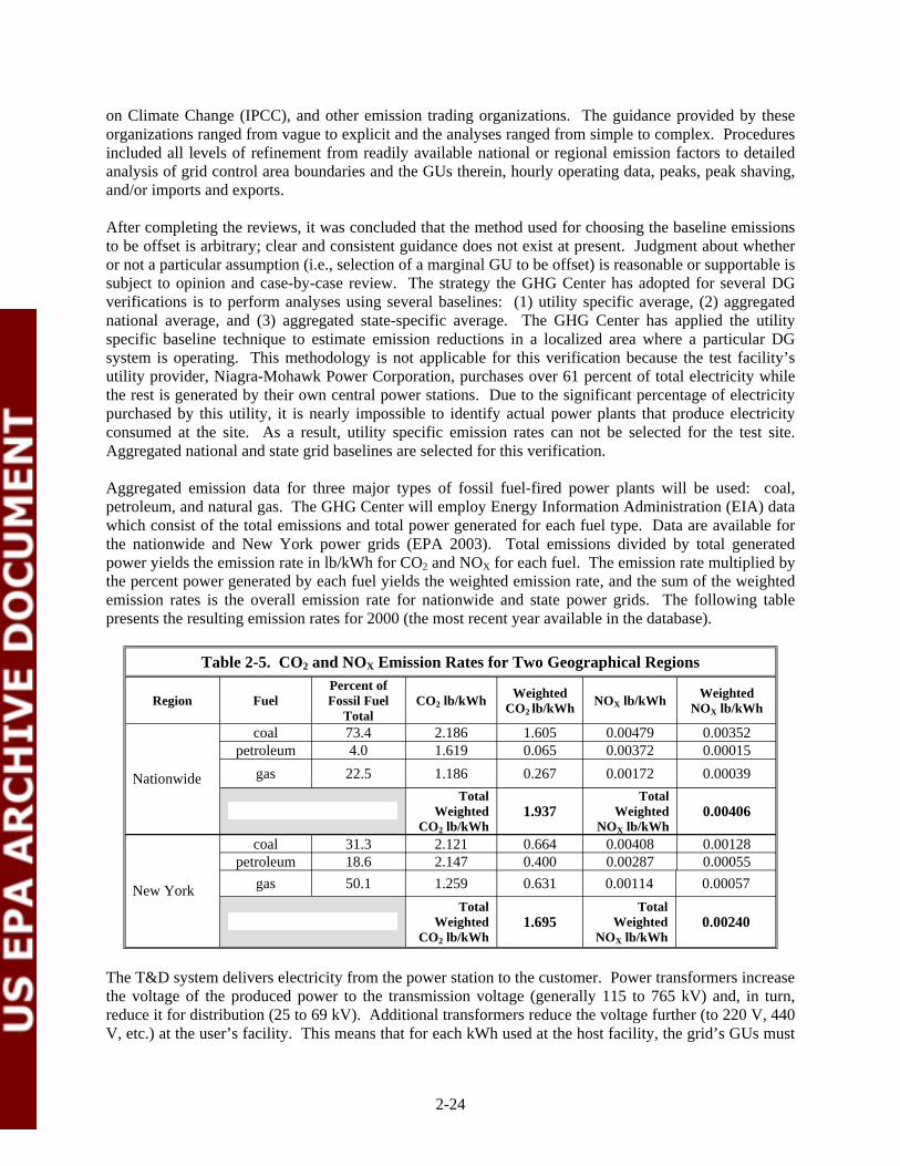
on Climate Change (IPCC), and other emission trading organizations. The guidance provided by these organizations ranged from vague to explicit and the analyses ranged from simple to complex. Procedures included all levels of refinement from readily available national or regional emission factors to detailed analysis of grid control area boundaries and the GUs therein, hourly operating data, peaks, peak shaving, and/or imports and exports.

After completing the reviews, it was concluded that the method used for choosing the baseline emissions to be offset is arbitrary; clear and consistent guidance does not exist at present. Judgment about whether or not a particular assumption (i.e., selection of a marginal GU to be offset) is reasonable or supportable is subject to opinion and case-by-case review. The strategy the GHG Center has adopted for several DG verifications is to perform analyses using several baselines: (1) utility specific average, (2) aggregated national average, and (3) aggregated state-specific average. The GHG Center has applied the utility specific baseline technique to estimate emission reductions in a localized area where a particular DG system is operating. This methodology is not applicable for this verification because the test facility’s utility provider, Niagra-Mohawk Power Corporation, purchases over 61 percent of total electricity while the rest is generated by their own central power stations. Due to the significant percentage of electricity purchased by this utility, it is nearly impossible to identify actual power plants that produce electricity consumed at the site. As a result, utility specific emission rates can not be selected for the test site. Aggregated national and state grid baselines are selected for this verification.

Aggregated emission data for three major types of fossil fuel-fired power plants will be used: coal, petroleum, and natural gas. The GHG Center will employ Energy Information Administration (EIA) data which consist of the total emissions and total power generated for each fuel type. Data are available for the nationwide and New York power grids (EPA 2003). Total emissions divided by total generated power yields the emission rate in lb/kWh for CO2 and NOX for each fuel. The emission rate multiplied by the percent power generated by each fuel yields the weighted emission rate, and the sum of the weighted emission rates is the overall emission rate for nationwide and state power grids. The following table presents the resulting emission rates for 2000 (the most recent year available in the database).

Table 2-5. CO2 and NOX Emission Rates for Two Geographical Regions

Region Fuel Percent of Fossil Fuel

Total CO2 lb/kWh Weighted

CO2 lb/kWh NOX lb/kWh Weighted NOX lb/kWh

Nationwide

coal 73.4 2.186 1.605 0.00479 0.00352 petroleum 4.0 1.619 0.065 0.00372 0.00015

gas 22.5 1.186 0.267 0.00172 0.00039 Total

Weighted CO2 lb/kWh

1.937 Total

Weighted NOX lb/kWh

0.00406

New York

coal 31.3 2.121 0.664 0.00408 0.00128 petroleum 18.6 2.147 0.400 0.00287 0.00055

gas 50.1 1.259 0.631 0.00114 0.00057 Total

Weighted CO2 lb/kWh

1.695 Total

Weighted NOX lb/kWh

0.00240

The T&D system delivers electricity from the power station to the customer. Power transformers increase the voltage of the produced power to the transmission voltage (generally 115 to 765 kV) and, in turn, reduce it for distribution (25 to 69 kV). Additional transformers reduce the voltage further (to 220 V, 440 V, etc.) at the user’s facility. This means that for each kWh used at the host facility, the grid’s GUs must

2-24

provide additional power to overcome the transformer, power line, and other losses. Federal Energy Regulatory Commission data (FERC 1999) indicate that in 1999, Niagara-Mohawk Power Corporation dispositioned 37,142,890 MWh of power while 1,642,346 MWh were lost. This equates to an approximate 4.4 percent T&D loss and means that for every kilowatt-hour generated and used by the host facility’s CHP, grid-connected GUs would have had to provide 1.044 kWh.

Power grid emission offsets, therefore, are based on the number of kilowatt-hours generated by the on-site CHP, line losses, and the grid emission rate for CO2 or NOX as shown in Equation 20.

EGRID = kWhCHP * ERGRID 044.1 * (Eqn. 20)

Where: EGRID = Grid CO2 or NOX emissions offset by the CHP, lbs kWhCHP = CHP system (projected or proven) power generated, kWh ERGRID = CO2 or NOX emission rates from Table 2-5, lb/kWh 1.044 = Total T&D losses

The resulting EGRID value will be used to estimate CO2 and NOX emission reductions according to Equation 17.

2-25

(this page intentionally left blank)

2-26

3.0 DATA QUALITY

3.1 BACKGROUND

The GHG Center selects methodologies and instruments for all verifications to ensure a stated level of data quality in the final results. The GHG Center specifies data quality objectives (DQOs) for each verification parameter before testing commences as a statement of data quality. Each test measurement that contributes to the determination of a verification parameter has stated Data Quality Indicator (DQI) goals, which, if met, ensure achievement of that parameter’s DQO.

The establishment of DQOs begins with the determination of the desired level of confidence in the verification parameters. Table 3-1 summarizes the DQOs for each verification parameter. The next step is to identify all measured values, which affect the verification parameter, and determine the levels of error which can be tolerated. The DQI goals, most often stated in terms of measurement accuracy, precision, and completeness, are used to determine if the stated DQOs are satisfied.

Table 3-1. Verification Parameter DQOs

Parameter Total Measurement Errora

(±) Absolute Relative

Power and Heat Production Performance Electrical power output at selected loads (kW) 0.6b kW 1.0 c % Electrical efficiency at selected loads (%) 0.43 % 1.6 d % Heat recovery rate at selected loads (Btu/hr) 6,415 Btu/hr 1.7 d % Thermal energy efficiency at selected loads (%) 0.88 % 1.7 d % Total CHP system efficiency (%) 1.82 % 1.2 d %

Power Quality Performance Electrical frequency (Hz) 0.006 Hz 0.01 % Voltage (VAC) 4.85 V 1.0c % Power factor (%) TBD 0.5 % Voltage and current THD (%) TBD 1.0 %

Emissions Performance Data Quality Indicators CO, NOX , CO2, and SO2 concentration (ppmv, %) TBD 2.0 % CH4, NH3, THC, and TRS, (ppmv) TBD 5.0 % TPM concentration (mg/dscm) 1 mg/dscm 1 mg/dscm a Bold column entries are DQOs; non-bold column entries are for information purposes b Assumes full load operation 120 kW: 480 V, 250 A c Includes 0.1 percent meter error and 1.0 percent current transformer (CT) error d Calculated composite error described in Section 3.3 TBD = to be determined

The following sections describe the data quality assessment process for each verification parameter. This includes a discussion of key measurements that contribute to the determination of the verification parameters, how measurement uncertainties affect their determination, and the resulting DQO. Each section consists of a listing and discussion of DQI goals and QA/QC checks that will be performed to verify the DQI goals are met, and how the DQOs will be reconciled.

3-1

3.2 ELECTRICAL POWER OUTPUT AND POWER QUALITY

The ION power meter will measure electrical power output and power quality. The inherent instrument error constitutes the DQO for power output, frequency, voltage, power factor, and THD as listed in Table 3-1. Table 3-2 summarizes the instrument specifications, DQI goals, and the primary method of evaluating the DQI goals achieved for each measurement. Factory calibrations, sensor function checks, and reasonableness checks in the field (listed in Tables 3-2 and 3-3) will document achievement of the DQI goals. Some of the QA/QC procedures to be performed are described below.

The power meter manufacturer will issue a calibration certificate which shows compliance with IEC 687 S0.2 and ANSI C12.20 CA0.2. Consistent with ISO 9002-1994 requirements, the manufacturer will supply calibration documents, which certify NIST traceability. The GHG Center will review the certificate and traceability records to ensure that the instrument meets or exceeds the accuracy specifications listed in Table 3-2. Note that the accuracy standard for power kW, compounded with the ± 1.0 percent accuracy specification for the current transformers, yields the ± 1.0 percent DQO specified in Table 3-1.

The power meter is designed and marketed for electric utility custody transfer applications. Its calibration records are reported to be valid for a minimum of one year of use, provided the manufacturer-specified installation and setup procedures are followed. GHG Center personnel will follow installation, setup, and QC procedures detailed in Appendices A-10 and A-11.

GHG Center personnel will perform checks in the field for two key measurements – voltage and current output – which are directly related to the power output measurement. These checks are intended to verify proper field wiring and function of the meter. The Field Team Leader will measure distribution panel voltage and current at the beginning of the verification period. He will use a digital multimeter (DMM) and compare voltage and current readings to the power meter readings as recorded by the DAS. The Field Team Leader will obtain a minimum of five individual voltage and current readings for the given load. The power meter voltage and current accuracies are ± 1.0 percent while the DMM is ± 1 percent. The percent difference between the DMM reading and the power meter reading should be within ± 1.4 percent for voltage and current (± 1.4 percent is the propagated error of the two measurements). In these cases, the power meter will be deemed to be functioning properly.

Comparisons of the power meter readings as recorded by the GHG Center’s DAS with the power output recorded by the PC25 control panel will constitute the reasonableness check. The power meter and control panel readout should indicate between 50 and 60 kW at full load.

3-2

Table 3-2. Measurement Instrument Specifications and DQI Goals Data Quality Indicator Goals

Measurement Variable Operating Range Expected in Field

Instrument Type /

Manufacturer

Instrument Range

Instrument Rated Accuracy

Frequency of Measurements Accuracya Completeness

How Verified / Determined

(see Table 3-3)

Electrical Power Output and Quality

Power 0 to 60 kW

Electric Meter/ Power Measurements 7600 ION

0 to 260 kW ± 1.0c % reading

DAS records 1-min averages

± 1.0 % readingc

95 % of all 1-min data collected during each load test run must be valid

Review manufacturer calibration certificates, Perform sensor function checks in field, Conduct reasonableness checks for voltage, current, and DAS

Voltage 480 V, 3 phase 0 to 600 V ± 1.0 % reading ± 1.0 % reading

Frequency 60 Hz 57 to 63 Hz ± 0.01 % reading ± 0.01 % reading

Current 0 to 250 amps 0 to 250 amps ± 1.0 % reading ± 1.0 % reading

Voltage THD 0 to 100 % 0 to 100 % ± 1 % FS ± 1 % FS

Current THD 0 to 100 % 0 to 100 % ± 1 % FS ± 1 % FS

Power Factor 0 to 1.0 0 to 1.0 ± 0.5 % reading ± 0.5 % reading

Heat Recovery

Fluid Flow Rate 20 to 80 gpm Controlotron Model 1010EPTRE

0 to 100 gpm ±1.5 % reading

DAS records 1-min averages

± 1.5 % of reading

Review manufacturer’s NIST traceable calibration records, Perform independent check of RTDs

Supply and Return Temperature

100 - 150 oF -40 to 250 oF ± 0.2 oF ± 1.5 o F

Ambient Meteorological Conditions

Ambient Temperatureb 20 to 70 oF

Vaisala HMD 60Y0

-40 to 140 oF ± 1 oF

DAS records 1-min averages

± 1 o F 95 % of all 1-min data collected during each load test run must be valid

Review manufacturer calibration certificates, Perform independent check of temperature and pressure sensors

Relative Humidityb 0 to 100 % 0 to 100 %

± 2 % 0 to 90 % (RH), ± 3 % 90 to 100 % (RH)

± 3 %

Ambient Pressure 13 to 16 psia SETRA Model

280E 0 to 25 in. Hg ± 0.1 % FS ± 0.1 % FS

(continued)

3-3

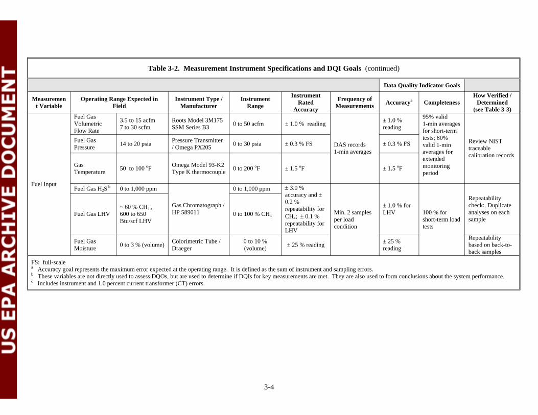
Table 3-2. Measurement Instrument Specifications and DQI Goals (continued)

Data Quality Indicator Goals

Measuremen t Variable

Operating Range Expected in Field

Instrument Type / Manufacturer

Instrument Range

Instrument Rated

Accuracy

Frequency of Measurements Accuracya Completeness

How Verified / Determined

(see Table 3-3)

Fuel Input

Fuel Gas Volumetric Flow Rate

3.5 to 15 acfm 7 to 30 scfm

Roots Model 3M175 SSM Series B3 0 to 50 acfm ± 1.0 % reading

DAS records 1-min averages

± 1.0 % reading

95% valid 1-min averages for short-term tests; 80% valid 1-min averages for extended monitoring period

Review NIST traceable calibration records

Fuel Gas Pressure 14 to 20 psia Pressure Transmitter

/ Omega PX205 0 to 30 psia ± 0.3 % FS ± 0.3 % FS

Gas Temperature 50 to 100 oF Omega Model 93-K2

Type K thermocouple 0 to 200 oF ± 1.5 oF ± 1.5 oF

Fuel Gas H2S b 0 to 1,000 ppm

Gas Chromatograph / HP 589011

0 to 1,000 ppm ± 3.0 % accuracy and ± 0.2 % repeatability for CH4; ± 0.1 % repeatability for LHV

Min. 2 samples per load condition

± 1.0 % for LHV 100 % for

short-term load tests

Repeatability check: Duplicate analyses on each sample

Fuel Gas LHV ~ 60 % CH4 , 600 to 650 Btu/scf LHV

0 to 100 % CH4

Fuel Gas Moisture 0 to 3 % (volume) Colorimetric Tube /

Draeger 0 to 10 % (volume) ± 25 % reading ± 25 %

reading

Repeatability based on back-to-back samples

FS: full-scale a Accuracy goal represents the maximum error expected at the operating range. It is defined as the sum of instrument and sampling errors. b These variables are not directly used to assess DQOs, but are used to determine if DQIs for key measurements are met. They are also used to form conclusions about the system performance. c Includes instrument and 1.0 percent current transformer (CT) errors.

3-4

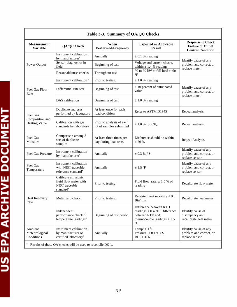
Table 3-3. Summary of QA/QC Checks

Measurement Variable QA/QC Check When

Performed/Frequency Expected or Allowable

Result

Response to Check Failure or Out of

Control Condition

Power Output

Instrument calibration by manufacturera Annually ± 0.1 % reading

Identify cause of any problem and correct, or replace meter

Sensor diagnostics in field Beginning of test Voltage and current checks

within ± 1.4 % reading

Reasonableness checks Throughout test 50 to 60 kW at full load at 60 °F

Fuel Gas Flow Rate

Instrument calibration a Prior to testing ± 1.0 % reading

Identify cause of any problem and correct, or replace meter

Differential rate test Beginning of test ± 10 percent of anticipated value

DAS calibration Beginning of test ± 1.0 % reading

Fuel Gas Composition and Heating Value

Duplicate analyses performed by laboratory

At least once for each load condition Refer to ASTM D1945 Repeat analysis

Calibration with gas standards by laboratory

Prior to analysis of each lot of samples submitted ± 1.0 % for CH4 Repeat analysis

Fuel Gas Moisture

Comparison among 3 sets of duplicate samples

At least three times per day during load tests

Difference should be within ± 20 % Repeat Analysis

Fuel Gas Pressure Instrument calibration by manufacturera Annually ± 0.3 % FS

Identify cause of any problem and correct, or replace sensor

Fuel Gas Temperature

Instrument calibration with NIST traceable reference standarda

Annually ± 1.5 oF Identify cause of any problem and correct, or replace sensor

Heat Recovery Rate

Calibrate ultrasonic fluid flow meter with NIST traceable standarda

Prior to testing Fluid flow rate: ± 1.5 % of reading Recalibrate flow meter

Meter zero check Prior to testing Reported heat recovery < 0.5 Btu/min Recalibrate heat meter

Difference between RTD Independent readings < 0.4 °F. Difference Identify cause of performance check of Beginning of test period between RTD and discrepancy and temperature readingsa thermocouple readings < 1.5 recalibrate heat meter

°F.

Ambient Instrument calibration Temp: ± 1 oF Identify cause of any Meteorological by manufacturer or Annually Pressure: ± 0.1 % FS problem and correct, or Conditions certified laboratorya RH: ± 3 % replace sensor

a Results of these QA checks will be used to reconcile DQIs.

3-5

3.3 EFFICIENCY

Electrical, thermal, and total CHP system efficiency parameters require determination of electrical power output, recovery rate, and fuel heat input. The efficiency DQOs were presented earlier in Table 3-1. Determination of these errors requires propagation of errors for one or more individual measurements, each with their own characteristic absolute and relative errors. These errors compound into an overall uncertainty for each verification parameter, which is the DQO for that parameter. Errors compound differently, depending on the algebraic operation required for the overall determination (Skoog 1982).

In general, for measurements which are added to or subtracted from each other, their absolute errors compound as follows:

2 2 (Eqn. 21)+, err abs c = err1 err2

Relative error, then, is:

err ,abs c (Eqn. 22), err rel c =value1 +value2

Where: errc,abs = Compounded error, absolute err1 = Error in first added value, absolute value err2 = Error in second added value, absolute value errc,rel = Compounded error, relative value1 = First added value value2 = Second added value

For measurements which are multiplied or divided by each other, their relative errors compound as follows:

2

2

2

2

1

1 , ⎟⎟

⎠

⎞ ⎜⎜ ⎝

⎛ +⎟⎟

⎠

⎞ ⎜⎜ ⎝

⎛ =

value err

value err

err rel c (Eqn. 23)

Where: errc,rel = Compounded error, relative err1 = Error in first multiplied (or divided) value, absolute value err2 = Error in second multiplied (or divided) value, absolute value value1 = First multiplied (or divided) value value2 = Second multiplied (or divided) value

Table 3-4 applies the concepts summarized in Equations 21 and 23 to estimate the compounded errors in the electrical efficiency. The table includes the contributing measurements, expected measured values, instrument/compounded errors, and reference equations. The resulting DQO is stated as an overall compounded absolute error or relative error in percent. Overall compounded error in thermal and total CHP efficiencies are determined using the same procedures shown here for electrical efficiency.

3-6

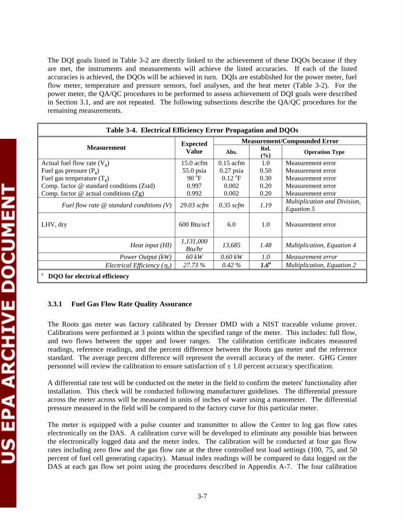
The DQI goals listed in Table 3-2 are directly linked to the achievement of these DQOs because if they are met, the instruments and measurements will achieve the listed accuracies. If each of the listed accuracies is achieved, the DQOs will be achieved in turn. DQIs are established for the power meter, fuel flow meter, temperature and pressure sensors, fuel analyses, and the heat meter (Table 3-2). For the power meter, the QA/QC procedures to be performed to assess achievement of DQI goals were described in Section 3.1, and are not repeated. The following subsections describe the QA/QC procedures for the remaining measurements.

Table 3-4. Electrical Efficiency Error Propagation and DQOs

Measurement Expected Value

Measurement/Compounded Error Abs. Rel.

(%) Operation Type

Actual fuel flow rate (Vg) Fuel gas pressure (Pg) Fuel gas temperature (Tg) Comp. factor @ standard conditions (Zstd) Comp. factor @ actual conditions (Zg)

15.0 acfm 55.0 psia

90 oF 0.997 0.992

0.15 acfm 0.27 psia 0.12 oF 0.002 0.002

1.0 0.50 0.30 0.20 0.20

Measurement error Measurement error Measurement error Measurement error Measurement error

Fuel flow rate @ standard conditions (V) 29.03 scfm 0.35 scfm 1.19 Multiplication and Division, Equation 5

LHV, dry 600 Btu/scf 6.0 1.0 Measurement error

Heat input (HI) 1,131,000 Btu/hr 13,685 1.48 Multiplication, Equation 4

Power Output (kW) 60 kW 0.60 kW 1.0 Measurement error Electrical Efficiency (ηe) 27.73 % 0.42 % 1.6a Multiplication, Equation 2

a DQO for electrical efficiency

3.3.1 Fuel Gas Flow Rate Quality Assurance

The Roots gas meter was factory calibrated by Dresser DMD with a NIST traceable volume prover. Calibrations were performed at 3 points within the specified range of the meter. This includes: full flow, and two flows between the upper and lower ranges. The calibration certificate indicates measured readings, reference readings, and the percent difference between the Roots gas meter and the reference standard. The average percent difference will represent the overall accuracy of the meter. GHG Center personnel will review the calibration to ensure satisfaction of ± 1.0 percent accuracy specification.

A differential rate test will be conducted on the meter in the field to confirm the meters' functionality after installation. This check will be conducted following manufacturer guidelines. The differential pressure across the meter across will be measured in units of inches of water using a manometer. The differential pressure measured in the field will be compared to the factory curve for this particular meter.

The meter is equipped with a pulse counter and transmitter to allow the Center to log gas flow rates electronically on the DAS. A calibration curve will be developed to eliminate any possible bias between the electronically logged data and the meter index. The calibration will be conducted at four gas flow rates including zero flow and the gas flow rate at the three controlled test load settings (100, 75, and 50 percent of fuel cell generating capacity). Manual index readings will be compared to data logged on the DAS at each gas flow set point using the procedures described in Appendix A-7. The four calibration

3-7

points will be used to develop the calibration curve, which will then be applied to the gas flow data stored on the DAS. A linear regression of the calibration curve that falls within 1 percent of the mean of the three averaged values at each flow rate compared with the meter index will indicate a gas flow rate accuracy at the DAS of ± 1 percent.

3.3.2 Gas Pressure and Barometric Pressure Quality Assurance

The Setra ambient pressure transducer and the Omega gas pressure transmitter are calibrated annually. The resulting calibration certificates are NIST-traceable; GHG Center personnel will review the calibration to ensure satisfaction of the accuracy specifications for each unit.

Reasonableness checks will be performed in the field by comparing the Omega gas pressure readings with the Setra readings. All pressure sensors will be exposed to atmospheric conditions. Agreement of the two units within 0.2 psia will show that the pressure sensors are operating properly.

3.3.3 Gas Temperature and Ambient Temperature Quality Assurance

The Omega gas temperature sensor and the Vaisala ambient temperature/RH sensor will be calibrated prior to testing. The resulting calibration certificates will be NIST-traceable. GHG Center personnel will review the calibration to ensure satisfaction of the ± 1.5 °F at 90 oF specification for the gas temperature sensor, and the ± 1 oF specification for ambient temperature.

3.3.4 Fuel Gas Analyses Quality Assurance

PTC-22 specifies that the fuel heating value be accurate to ± 1.0 percent or better. This will be the DQI for the fuel analysis. Field personnel will collect fuel gas samples as described in Section 2.2.3.5 and submit them for laboratory analysis. The laboratory will perform compositional analysis by ASTM D1945 and calculate LHV and HHV by ASTM D3588.

ASTM D1945 repeatability directly affects the ASTM D3588 LHV and HHV data quality. Provided the D1945 repeatability criteria are met, the LHV and HHV repeatability is approximately 1.2 Btu per 1000 ft3, or about 0.1 percent. The ASTM D1945 allowable method error during calibration is ± 1.0 percent of the reference value for each gas component. The reference standard will be a NIST-traceable natural gas reference standard of known concentration.

The compounded accuracy of the two methods, including repeatability, allowable instrument error, and the maximum permitted calibration error, is therefore 1.0 percent. Achievement of proper calibrations and repeatability imply that use of these two ASTM methods will ensure that LHV and HHV data are accurate to ± 1.0 percent or better.

At the laboratory, analysts will challenge the instrumentation at least weekly with a gas reference standard. The result for each gas component must be within ± 1.0 percent. The laboratory will also analyze each fuel gas sample in duplicate. The duplicate analyses must conform to the ASTM D1945 repeatability guidelines for each gas component.

3-8

3.3.5 Heat Recovery Rate Quality Assurance

Tables 3-2 and 3-3 summarize the DQIs and QA/QC checks associated with this verification parameter. The following paragraphs discuss these checks. The GHG Center will obtain factory calibrations for the flow transducers and RTDs to ensure the energy meters' accuracy requirements are met. The flow transducer is calibrated by Controlotron at the factory following their CS2 Flow Through Calibration Procedure. In general, the meter is mounted on a specific type and size of pipe as requested by the Center following standard installation procedures. A series of tests are then conducted by passing known amounts of water through the pipe and comparing the meter response with the reference standard. The reference standard consists of a NIST traceable temperature sensor, timer, balance, and reference weights. This meter was calibrated on 2-inch carbon steel pipe and 1.5-inch copper pipe in October 2002.

The meter zero check verifies a zero reading by the meter when the CHP system is not in operation. The energy meter’s fluid index check uses the ultrasonic signal transit time to verify the meter installation integrity. The meter’s software uses a series of look-up tables to assign a reference transit time signal based on input parameters which includes tubing specifications and fluid composition. The Field Team Leader will compare the actual transit-time signal to the reference value After installation of the meter components. Differences between the actual and reference values in excess of 5.0 percent indicate an installation or programming error and a need for corrective action.

The Field Team Leader will independently verify RTD accuracy in the field. He will remove the RTDs from the fluid tubing and place them in an ice water bath along with thermocouples of known accuracy. Temperature readings from both sensors will be recorded for comparison. He will then repeat the procedure in a hot water bath. If the average differences in temperature readings are greater than 1.5 oF, the meter RTDs will be sent for re-calibration. Appendix A-8 contains the field data form.

3.4 EMISSION MEASUREMENTS QA/QC PROCEDURES

The GHG Center will employ the EPA Reference Methods listed in Table 2-3 to determine emission rates of criteria pollutants and greenhouse gases. Table 3-6 summarizes the instrument type or measurement method, accuracy, and DQIs for this verification. The Reference Methods specify the sampling methods, calibrations, and data quality checks that must be followed to achieve a data set that meets the DQOs. These procedures ensure the quantification of run-specific instrument and sampling errors and that runs are repeated if the specific performance goals are not met. The GHG Center will assess emissions data quality, integrity, and accuracy through these system checks and calibrations.

In past verifications, the DQI for TPM emissions was established as ± 5 percent. For this test however, the overall uncertainty in emission rates may be much higher due to the limited the extremely low particulate concentrations expected and the sensitivity of the gravimetric analyses. Therefore, the specified DQI for TPM is based on the generally accepted method detection limit of ± 1 milligram per dry standard cubic meter (mg/dscm).

Specific procedures to be conducted during this test are outlined in the following sections and summarized in Table 3-7. Satisfaction and documentation of each of the calibrations and QC checks will verify the accuracy and integrity of the measurements with respect to the DQIs listed in Table 3-7.

3.4.1 NOx Emissions Quality Assurance

NOx Analyzer Interference Test

3-9

In accordance with Method 20, an interference test will be conducted on the NOx analyzer once before the testing begins. This test is conducted by injecting the following calibration gases into the analyzer:

• CO – 500 ± 50 ppm in balance N2

• SO2 – 200 ± 20 ppm in N2

• CO2 – 10 ± 1 % in N2

• O2 – 20.9 ± 1 %

For acceptable analyzer performance, the sum of the interference responses to all of the interference test gases must be ≤ 2 percent of the analyzer span value. Analyzers failing this test will be repaired or replaced.

NO2 Converter Efficiency Test

The NOx analyzer converts any NO2 present in the gas stream to NO prior to gas analysis. A converter efficiency test must be conducted prior to beginning the testing. This procedure is conducted by introducing to the analyzer a mixture of mid-level calibration gas and air. The analyzer response is recorded every minute thereafter for 30 minutes. If the NO2 to NO conversion is 100 percent efficient, the response will be stable at the highest peak value observed. If the response decreases by more than 2 percent from the peak value observed during the 30-minute test period, the converter is faulty. A NOx analyzer failing the efficiency test will be either repaired or replaced prior to testing.

NOx and THC Sampling System Calibration Error and Drift

The sampling system calibration error test must be conducted prior to the start of the first test on each day of testing the NOX sampling system. Note that the same procedures must be performed on the THC sampling system. The calibration is conducted by sequentially introducing a suite of calibration gases to the sampling system at the sampling probe, and recording the system response. Calibrations will be conducted on all analyzers using EPA Protocol No. 1 calibration gases. Four NOX, and THC calibration gases are required including zero, 20 to 30 percent of span, 40 to 60 percent of span, and 80 to 90 percent of span. The maximum allowable error in response to any of the calibration gases is ± 2 percent of span for NOX and ± 5 percent of span for THC.

At the conclusion of each test the zero and mid-level calibration gases are again introduced to the sampling systems at the probe and the response is recorded. System response is compared to the initial calibration error to determine sampling system drift. Drifts in excess of ± 2 percent for NOX and ± 3 percent for THC are unacceptable and the test will be repeated.

NOX Audit Gas

The NOX analyzer will be operated on a full-scale range of 0 to 25 ppm. It is possible that turbine emissions might be at the low end of the analytical range (5 ppm or less). To evaluate the NOX sampling system accuracy at low concentrations, the GHG Center will provide an EPA Protocol 1 calibration gas of approximately 5 ppm to be used as a blind audit of the NOX sampling system. Without revealing the certified NOX concentration to the emissions testing contractor, the audit gas will be introduced to the sampling system at the probe tip and a stable system response will be recorded. System error will be calculated as follows:

[(system error percent span) = {system response ppm) / audit gas ppm)] / span} x 100 (Eqn. 24)

3-10

The sampling system response must be within ± 5 percent of the certified audit gas concentration. Corrective action will be taken to resolve sampling system bias if the response exceeds this specification. Results of this audit will be presented in the verification report and serves as a performance evaluation audit (PEA).

3.4.2 CO, CO2, O2, and SO2 Emissions Quality Assurance

Calibration Error, System Bias, and Calibration Drift Tests

These calibrations will be conducted to verify accuracy of CO, CO2, O2, and SO2 measurements. The calibration error test is conducted at the beginning of each day of testing. A suite of calibration gases is introduced directly to each analyzer and analyzer responses are recorded. EPA Protocol 1 calibration gases must be used for these calibrations. Three gases will be used for CO2, O2, and SO2 including zero, 40 to 60 percent of span, and 80 to 100 percent of span. Four gases will be used for CO including zero and approximately 30, 60, and 90 percent of span. The maximum allowable error in monitor response to any of the calibration gases is ± 2 percent of span.

Before and after each test, the zero and mid-level calibration gases will be introduced to the sampling system at the probe and the response recorded. System bias will then be calculated by comparing the responses to the calibration error responses recorded earlier. System bias must be less than ± 5 percent of span for each parameter for the sampling system to be acceptable. The pre- and post-test system bias calibrations will also be used to calculate drift for each monitor. Drifts in excess of ± 3 percent will be considered unacceptable and the test will be repeated.

3-11

Table 3-6. Instrument Specifications and DQI Goals for Stack Emissions Testing

Instrument Specifications Data Quality Indicators

Measurement Variable Instrument Type or Method

Frequency of Measurements

Overall Sampling System Accuracy Completeness How Verified /

Determineda

NOX Concentrations

Chemilumenescense analyzer

± 2 % FS includes sampling system bias corrections)

CO Concentrations NDIR analyzer ± 2 % FS (includes sampling system bias

Microturbine Emissions

1-minute averages (DAS polls analyzer outputs at 5­second intervals)

corrections)

100 % 3 valid runs at each specified load)

Follow EPA Method calibration and system performance check criteria

TRS Concentrations Pulsed fluorescent analyzer ± 5 % FS

NH3 Concentrations Ion chromatograph ± 5 % FS

SO2 Concentrations Pulsed fluorescent analyzer

± 2 % FS (includes sampling system bias corrections)

THC Concentrations FID analyzer ± 5 % FS

TPM Concentrations Gravimetric ± 1 mg/dscm

CO2 / O2 Levels; Stack Gas Molecular Weight

NDIR (CO2) / paramagnetic or equivalent (O2)

± 2 % FS (includes sampling system bias corrections)

CH4 Concentrations GC / FID

Once per test run ± 5 % FS

Stack Gas Flow Rate Pitot and Thermocouple ± 5 % FS

Water Content Gravimetric Once per load condition ± 5 % FS

a For a full description, see Table 3-4.

3-12

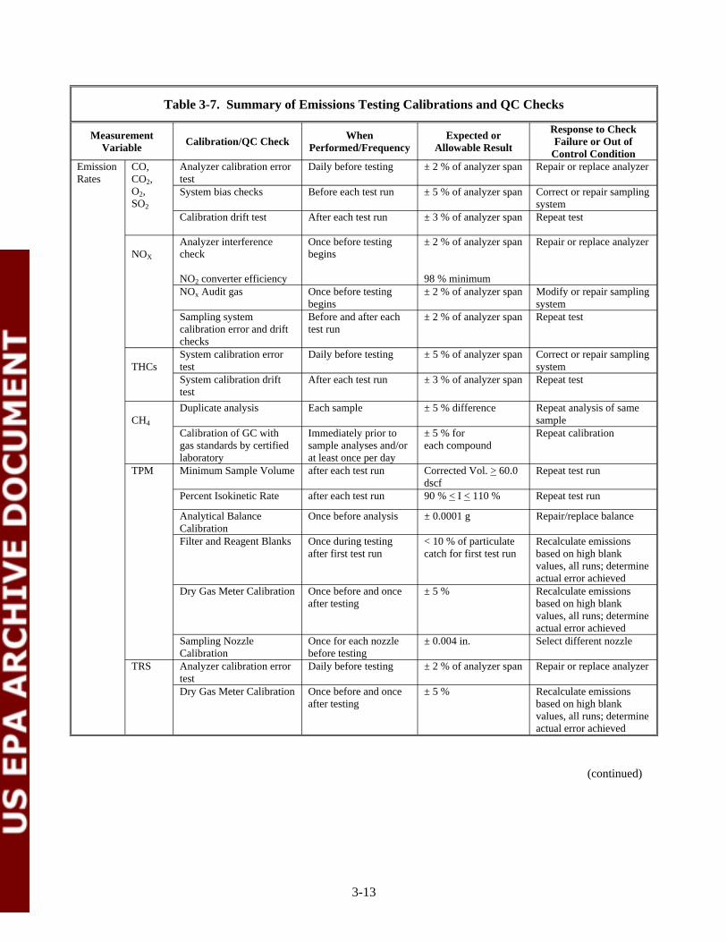
Table 3-7. Summary of Emissions Testing Calibrations and QC Checks

Measurement Variable Calibration/QC Check When

Performed/Frequency Expected or

Allowable Result

Response to Check Failure or Out of

Control Condition Emission CO, Analyzer calibration error Daily before testing ± 2 % of analyzer span Repair or replace analyzer Rates CO2,

O2, SO2

test System bias checks Before each test run ± 5 % of analyzer span Correct or repair sampling

system Calibration drift test After each test run ± 3 % of analyzer span Repeat test

Analyzer interference Once before testing ± 2 % of analyzer span Repair or replace analyzer NOX check begins

NO2 converter efficiency 98 % minimum NOx Audit gas Once before testing ± 2 % of analyzer span Modify or repair sampling

begins system Sampling system Before and after each ± 2 % of analyzer span Repeat test calibration error and drift test run checks

THCs System calibration error test

Daily before testing ± 5 % of analyzer span Correct or repair sampling system

System calibration drift After each test run ± 3 % of analyzer span Repeat test test

CH4

Duplicate analysis Each sample ± 5 % difference Repeat analysis of same sample

Calibration of GC with Immediately prior to ± 5 % for Repeat calibration gas standards by certified sample analyses and/or each compound laboratory at least once per day

TPM Minimum Sample Volume after each test run Corrected Vol. > 60.0 dscf

Repeat test run

Percent Isokinetic Rate after each test run 90 % < I < 110 % Repeat test run

Analytical Balance Calibration

Once before analysis ± 0.0001 g Repair/replace balance

Filter and Reagent Blanks Once during testing after first test run

< 10 % of particulate catch for first test run

Recalculate emissions based on high blank values, all runs; determine actual error achieved

Dry Gas Meter Calibration Once before and once after testing

± 5 % Recalculate emissions based on high blank values, all runs; determine actual error achieved

Sampling Nozzle Once for each nozzle ± 0.004 in. Select different nozzle Calibration before testing

TRS Analyzer calibration error Daily before testing ± 2 % of analyzer span Repair or replace analyzer test Dry Gas Meter Calibration Once before and once

after testing ± 5 % Recalculate emissions

based on high blank values, all runs; determine actual error achieved

(continued)

3-13

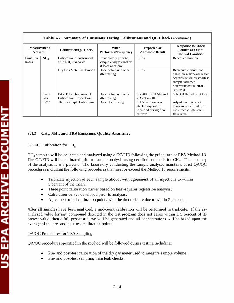
Table 3-7. Summary of Emissions Testing Calibrations and QC Checks (continued)

Measurement Variable Calibration/QC Check When

Performed/Frequency Expected or

Allowable Result

Response to Check Failure or Out of

Control Condition Emission Rates

NH3 Calibration of instrument with NH3 standards

Immediately prior to sample analyses and/or at least once/day

± 5 % Repeat calibration

Dry Gas Meter Calibration Once before and once after testing

± 5 % Recalculate emissions based on whichever meter coefficient yields smallest sample volume; determine actual error achieved

Stack Gas Flow

Pitot Tube Dimensional Calibration / Inspection

Once before and once after testing

See 40CFR60 Method 2, Section 10.0

Select different pitot tube

Thermocouple Calibration Once after testing ± 1.5 % of average stack temperature recorded during final test run

Adjust average stack temperatures for all test runs; recalculate stack flow rates

3.4.3 CH4, NH3, and TRS Emissions Quality Assurance

GC/FID Calibration for CH4

CH4 samples will be collected and analyzed using a GC/FID following the guidelines of EPA Method 18. The GC/FID will be calibrated prior to sample analysis using certified standards for CH4. The accuracy of the analysis is ± 5 percent. The laboratory conducting the sample analyses maintains strict QA/QC procedures including the following procedures that meet or exceed the Method 18 requirements.

• Triplicate injection of each sample aliquot with agreement of all injections to within 5 percent of the mean;

• Three point calibration curves based on least-squares regression analysis; • Calibration curves developed prior to analysis; • Agreement of all calibration points with the theoretical value to within 5 percent.

After all samples have been analyzed, a mid-point calibration will be performed in triplicate. If the as­analyzed value for any compound detected in the test program does not agree within ± 5 percent of its pretest value, then a full post-test curve will be generated and all concentrations will be based upon the average of the pre- and post-test calibration points.

QA/QC Procedures for TRS Sampling

QA/QC procedures specified in the method will be followed during testing including:

• Pre- and post-test calibration of the dry gas meter used to measure sample volume; • Pre- and post-test sampling train leak checks;

3-14

The SO2 analyzer used to measure TRS concentrations will be calibrated using the calibration error procedures outlined in Section 3.4.2.

QA/QC Procedures for NH3 Sampling

QA/QC procedures specified in the method will be followed during testing including:

• Pre- and post-test calibration of the dry gas meter used to measure sample volume; • Pre- and post-test sampling train leak checks; • Collection, submittal, and analysis of a reagent blank.

Before the first test run, test operators will collect an aliquot of each sampling and recovery reagent from the storage containers to be used during testing. They will label these as “Trip Blanks” and analyze them along with other samples.

Collected NH3 samples will be shipped to a laboratory for analysis using an ion chromatograph (IC) equipped with conductivity detector. The IC is calibrated using a series of six internal standards that bracket the expected range of sample concentrations. The analytical system is then challenged with no less than three NIST traceable reference standards to evaluate analytical accuracy. The analysis accuracy must be within ± 5 percent of each of the standards, or the system must be repaired and/or recalibrated.

3.4.4 Gas Flow Rate and Particulate Emissions Quality Assurance

Pitot Tube Calibration

Determination of stack gas flow rate includes measurement of exhaust gas concentrations of O2, CO2, and water, velocity differential pressure across a pitot tube, and gas temperature. The GHG Field Team Leader will review O2 and CO2 instrumental analyzer data at the end of each test day. Review criteria will be as described previously for the instrumental analyzers. Stack gas moisture field data will also be reviewed to ensure proper procedures were followed (EPA Method 4).

Emissions test operators will certify that the pitot tubes meet applicable requirements for dimensional accuracy using the design criteria detailed in Method 2. Also in accordance with Method 2 calibration criteria, they will perform pre- and post-test thermocouple calibrations by subjecting the thermocouples used during testing to the average temperature found during testing and comparing the readings to a NIST-traceable reference thermometer. For acceptable results, the thermocouple reading must be within 1.5 percent of the reference thermometer. 40CFR60 Method 2, Section 10.3.1 contains thermocouple calibration procedures.

For a valid TPM sample, the minimum sample volume will be 60 dry standard cubic feet (dscf). The GHG Field Team Leader will review field data sheets for each test run to ensure that the proper sample volume was collected. Particulate matter must be sampled isokinetically; in general, this means that the velocity of the stack gas entering the sampling nozzle must be the same as the surrounding stack gas. Method 5 provides equations for computing the isokinetic sampling rate, I. The results are expressed as a percentage of the ideal rate. For these tests, the allowable variation is 90 percent < I < 110 percent of the ideal isokinetic sampling rate. Test operators will compute I at the conclusion of each test run, and the GHG Field Team Leader will review the calculation before proceeding with the next test run.

3-15

To minimize the possibility of sample contamination, sampling probes must have glass liners. Glass nozzles are preferred, but not required. All nozzles must be dimensionally calibrated; GHG Center personnel will review the calibration data while at the test site.

To minimize variability in the back half analysis, test operators will collect sampling filters, reagents and rinses in a clean environment and as expeditiously as possible. The Field Team Leader will observe these efforts for each test run. He will note the starting and ending times for particulate sample recovery and any problems in the Daily Test Log. Method 5 includes procedures for collecting and analyzing filter and reagent blanks. This Test Plan specifically requires filter and reagent blanks as follows:

Filter Blank Test operators will install an unused filter into the isokinetic sampling chain and conduct a normal leak check as specified in the Methods. This could be done in conjunction with the sample blank described below. They will recover the filter and analyze it along with the test run filters.

Reagent Blanks Before the first test run, test operators will collect a 200-ml aliquot of each sampling and recovery reagent from the storage containers to be used during testing. They will label these as “Trip Blanks” and analyze them along with other samples.

Before the first test run, test operators will charge the impinger train with the required sampling reagents. They will conduct a normal leak check as specified in the Methods. This could be done in conjunction with the Filter Blank described above. The sampling train will then be washed and sample recovered as if a normal test run had occurred. The recovered reagents will be labeled as “Sample Blank” including separate labeled bottles for “Probe/nozzle”; “Impinger Water”; “Impinger Acetone”; and “Impinger Methylene Chloride”, and analyzed along with the other samples.

Particulate Data Completeness and Reasonableness The GHG Field Team Leader will review and initial each field data sheet for each particulate sampling test run for completeness and reasonableness. The individual reference methods detail the data to be collected and the review criteria to be employed, but some points are emphasized here for specific methods.

Method 2c stack initial velocity traverse and cyclonic flow check forms must clearly depict the stack traverse points and cyclonic flow readings at those points. Probes and thermocouples must be uniquely identified and calibration information must be traceable to the probe ID. Method 4 (moisture content) impinger weight forms must include tare and final impinger weights and the total weight of moisture collected.

Method 5 (particulate sampling) forms must include entries for ambient temperature, stack static pressure, nozzle, probe, dry gas meter, and other sample train ID numbers. Barometric pressure must be noted for local conditions, uncorrected to sea level, and must include statements about the elevation difference between the instrument’s location and the stack sampling location. Calibration information must be traceable to the probe, nozzle, sampling train, and other ID’s. Leak check data must include vacuum (Hg), start reading and end reading of the dry gas meter, and a notation that the sample train conforms to leak check requirements.

All sample containers must be sealed and marked with unique identification numbers, which can be traced to each test run. Test operators will mark the outside of all liquid sample containers with a line at the liquid level contained in the bottle. Laboratory personnel will inspect the marks and note whether any fluid has been lost in transport and handling.

3-16

At the conclusion of the first emissions test run, test operators will calculate stack moisture content, molecular weight, velocity, volumetric flow, and percent isokinetic sampling rate. The GHG Center representatives will review the calculations before they authorize the following test runs. Comparison of the field data from the first run with following runs will show if the collected data are reasonable and consistent. These procedures and calibrations will provide documentation that the accuracy of each of the individual measurements conformed to Reference Method specifications. Knowing this, an overall uncertainty of ± 5 percent of reading is assigned for TPM determinations, based on propagation of the sum of the squares of the individual measurement errors (Shigehara 1970).

3.5 INSTRUMENT TESTING, INSPECTION, AND MAINTENANCE

The equipment used to collect verification data will be subject to the pre- and post-test QC checks discussed earlier. Before the equipment leaves the GHG Center or analytical laboratories, it will be assembled exactly as anticipated to be used in the field and fully tested for functionality. For example, all controllers, flow meters, computers, instruments, and other sub-components of the measurements system will be operated and calibrated as required by the manufacturer and/or this Test Plan. Any faulty sub­components will be repaired or replaced before being transported to the test site. A small amount of consumables and frequently needed spare parts will be maintained at the test site. Major sub-component failures will be handled on a case-by-case basis (e.g., by renting replacement equipment or buying replacement parts).

The instruments used to make gas flow rate measurements are new, having been purchased for this verification. They will be inspected at the GHG Center’s laboratory prior to installation in the field to ensure all parts are in good condition. The equipment used to make gas pressure and temperature, and the GHG Center’s Environmental Studies Group maintain ambient measurements. The mass flow meters, temperature, gas pressure, and other sensors will be submitted to the manufacturer for calibration prior to being transported to the test site.

3.6 INSPECTION/ACCEPTANCE OF SUPPLIES AND CONSUMABLES

Natural Gas Reference Standard gases will be used to calibrate the GC used for fuel analyses. The concentrations of components in the audit gas are certified within ± 2 percent of the tag value. Copies of the audit gas certifications will be available on-site during testing and archived at the GHG Center.

EPA Protocol gases will be used to calibrate the gaseous pollutant measurement system. Calibration gas concentrations meeting the levels stated in Section 2.4 will either be generated from high concentration gases for each target compound using a dilution system or supplied directly from gas cylinders. Per EPA Protocol gas specifications, the actual concentration must be within ± 2 percent of the certified tag value. Copies of the EPA Protocol gas certifications will be available on-site.

3-17

(this page intentionally left blank)

3-18

4.0 DATA ACQUISITION, VALIDATION, AND REPORTING

4.1 DATA ACQUISITION AND STORAGE

Test personnel will acquire the following types of data during the verification:

• Continuous measurements i.e., gas pressure, gas temperature, power output and quality, heat recovery, and ambient conditions, to be collected by the GHG Center’s DAS

• Fuel gas composition, heating value, compressibility factor, and moisture content from canister samples collected by the Field Team Leader and submitted to laboratory for analysis

• Volumetric gas flow measurements collected by the Field Team Leader • Emission measurements data collected by contractor and supervised by the Field

Team Leader.

The Field Team Leader will also take site photographs and maintain a Daily Test Log which includes the dates and times of setup, testing, teardown, and other activities.

The Field Team Leader will submit digital data files, gas analyses, chain of custody forms, and the Daily Test Log to the Project Manager. The Project Manager will initiate the data review, validation, and calculation process. These submittals will form the basis of the Verification Report which will present data analyses and results in table, chart, or text format as is suited to the data type. The Verification Report’s conclusions will be based on the data and the resulting calculations. The GHG Center will archive and store all data in accordance with the GHG Center QMP.

4.1.1 Continuous Measurements

An electronic DAS will collect and store continuous process and ambient meteorological data. Core components of the DAS are an Allen-Bradley (AB) Model SLC 5/05 programmable logic controller (PLC) and a Gladiator Unix-based data acquisition computer data server (TOGA). Figure 4-1 is a schematic of the DAS.

The PLC brings all analog and digital signals from the measurement sensors together into a single real­time data source. The DAS can accommodate any combination of up to 16 analog signal channels with 4 to 20 mA current or DC voltage inputs. Sensors can also provide digital signals via the ModBus network to the DF1 interface unit. This converts the ModBus data to the AB “DF1” protocol which is compatible with the PLC. The PLC nominally polls each sensor once per second and converts the signals to engineering units. It then computes 1-minute averages for export to the TOGA and applies a common time stamp to facilitate data synchronization of all measurements.

4-1

Figure 4-1. DAS Schematic

(s)

Remote or Local Connection Through Ethernet or Modem

4 - 20 MA current loops to analog output sensors

Modbus Sensors

Remote or Local Computer

Data Acquisition System

The TOGA data server records information from the PLC and contains the software for programming the PLC (i.e., data sampling rates, engineering unit conversions, calibration constants). Its UNIX operating system writes all PLC data to a My-SQL relational database for export to spreadsheet, graphics, and other programs. This database is ODBC-compliant, which means that almost any MS Windows program can use the data. The data server includes an external modem and Ethernet card for remote and local communications. During normal operations, the user accesses the data server with a portable laptop or remote computer (PC) via its communications port, Ethernet link, or telephone connection. Spreadsheets allow the user to download the entire database or only that portion which has been added since the last download. The user then conducts data queries i.e., for certain times, dates, and selected data columns on the downloaded data as needed.

During the verification testing, GHG Center personnel will configure the DAS to acquire the process variables listed in Table 4-1. Note that the Field Team Leader will acquire the CHP power command and date/time data manually at the start of each test run.

4-2

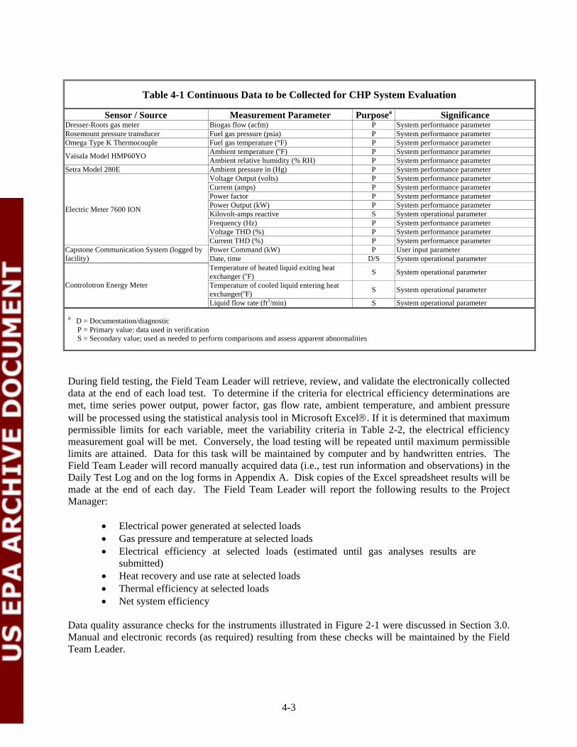
Table 4-1 Continuous Data to be Collected for CHP System Evaluation

Sensor / Source Measurement Parameter Purposea Significance Dresser-Roots gas meter Biogas flow (acfm) P System performance parameter Rosemount pressure transducer Fuel gas pressure (psia) P System performance parameter Omega Type K Thermocouple Fuel gas temperature (°F) P System performance parameter

Vaisala Model HMP60YO Ambient temperature (oF) P System performance parameter Ambient relative humidity (% RH) P System performance parameter

Setra Model 280E Ambient pressure in (Hg) P System performance parameter

Electric Meter 7600 ION

Voltage Output (volts) P System performance parameter Current (amps) P System performance parameter Power factor P System performance parameter Power Output (kW) P System performance parameter Kilovolt-amps reactive S System operational parameter Frequency (Hz) P System performance parameter Voltage THD (%) P System performance parameter Current THD (%) P System performance parameter

Capstone Communication System (logged by facility)

Power Command (kW) P User input parameter Date, time D/S System operational parameter

Controlotron Energy Meter

Temperature of heated liquid exiting heat exchanger (oF) S System operational parameter

Temperature of cooled liquid entering heat exchanger(oF) S System operational parameter

Liquid flow rate (ft3/min) S System operational parameter

a D = Documentation/diagnostic P = Primary value: data used in verification S = Secondary value; used as needed to perform comparisons and assess apparent abnormalities

During field testing, the Field Team Leader will retrieve, review, and validate the electronically collected data at the end of each load test. To determine if the criteria for electrical efficiency determinations are met, time series power output, power factor, gas flow rate, ambient temperature, and ambient pressure will be processed using the statistical analysis tool in Microsoft Excel®. If it is determined that maximum permissible limits for each variable, meet the variability criteria in Table 2-2, the electrical efficiency measurement goal will be met. Conversely, the load testing will be repeated until maximum permissible limits are attained. Data for this task will be maintained by computer and by handwritten entries. The Field Team Leader will record manually acquired data (i.e., test run information and observations) in the Daily Test Log and on the log forms in Appendix A. Disk copies of the Excel spreadsheet results will be made at the end of each day. The Field Team Leader will report the following results to the Project Manager:

• Electrical power generated at selected loads • Gas pressure and temperature at selected loads • Electrical efficiency at selected loads (estimated until gas analyses results are

submitted) • Heat recovery and use rate at selected loads • Thermal efficiency at selected loads • Net system efficiency

Data quality assurance checks for the instruments illustrated in Figure 2-1 were discussed in Section 3.0. Manual and electronic records (as required) resulting from these checks will be maintained by the Field Team Leader.

4-3

After the completion of all test runs, original field data forms, the Daily Test Log, and electronic copies of data output and statistical analyses will be stored at the GHG Center’s RTP office per guidelines described in the GHG Center’s QMP.

4.1.2 Emission Measurements

The emissions testing contractor will be responsible for all emissions data, QA log forms, and electronic files until they are accepted by the Field Team Leader. For pollutant quantified on-site with analyzers, the emissions contractor will use software to record the concentration signals from the individual monitors. The typical DAS records instrument output at one-second intervals, and averages those signals into 1-minute averages. At the conclusion of a test run, the pre-and post-test calibration results and test run values will be electronically transferred from the tester's DAS into a Microsoft Excel spreadsheet for data calculations and averaging.

The emissions contractor will report emission measurements results to the Field Team Leader as:

• Parts per million by volume (ppmv) • ppmv corrected to 15 percent O2

• Emission rate (lb/hr)

Upon completion of the field test activities, the emissions contractor will provide copies of records of calibration, pre-test checks, system response time, NO2 converter flow/efficiency, blind audit sample, and field test data to Field Team Leader prior to leaving the site. Testing for NH3, CH4, TRS, and TPM requires analytical procedures that are conducted off-site at a laboratory. The contractor will provide copies of sample chain-of-custody records, analytical data, and laboratory QA/QC documentation for these parameters after field activities are finished. Before leaving the site, the contractor will also provide copies of the field data logs that document collection of each of these samples, as well as QA/QC documentation for the equipment used in collection of these samples (e.g., pitot tubes, gas meters, thermocouples).

A formal report will be prepared by the contractor and submitted to GHG Center Field Team Leader within three weeks of completion of the field activities. The report will describe the test conditions, document all QA/QC procedures, include copies of calibrations, calibration gas, and the certification test results. Field data will be included as an appendix and an electronic copy of the report will be submitted. The submitted information will be stored at the GHG Center’s RTP office per guidelines defined in the QMP.

4.1.3 Off Site Analyses

Samples collected during field testing that will be analyzed off-site include samples of fuel gas, exhaust gas (for CH4), and impinger solutions (for NH3). Sampling and QA/QC procedures for each type of sample are discussed in Section 2.0. The Field Team Leader will maintain manual sampling logs and chain of custody records for each sample collected. Three separate analytical laboratories will be used. After the field test, the laboratories will submit results for each sample, calibration records, and repeatability test results to the Field Team Leader. Original lab reports and electronic copies of data output and statistical analyses will be stored at the GHG Center’s RTP office per guidelines described in the GHG Center’s QMP.

4-4

4.2 DATA REVIEW, VALIDATION, AND VERIFICATION

Data review and validation will primarily occur at the following stages:

• On-site -- by the Field Team Leader • Before writing the draft Verification Report -- by the Project Manager • During QA review of the draft Verification Report and audit of the data -- by the

GHG Center QA Manager

Figure 1-4 identifies the individuals who are responsible for data validation and verification. The Field Team Leader will be able to review, verify, and validate some data (i.e., DAS file data, reasonableness checks) while on-site. Other data, such as fuel LHV and fuel gas properties, must be reviewed, verified, and validated after testing has ended. The Project Manager holds overall responsibility for these tasks.

Upon review, all collected data will be classed as valid, suspect, or invalid. The GHG Center will employ the QA/QC criteria discussed in Section 3.0. Review criteria are in the form of factory and on-site calibrations, maximum calibration and other errors, and audit gas analyses results, and lab repeatability results. In general, valid results are based on measurements which meet the specified DQIs and QC checks, that were collected when an instrument was verified as being properly calibrated, and that are consistent with reasonable expectations (e.g., manufacturers’ specifications, professional judgment).

The data review process often identifies anomalous data. Test personnel will investigate all outlying or unusual values in the field as is possible. Anomalous data may be considered suspect if no specific operational cause to invalidate the data is found.

All data, valid, invalid, and suspect will be included in the Verification Report. However, report conclusions will be based on valid data only and the report will justify the reasons for excluding any data. Suspect data may be included in the analyses, but may be given special treatment as specifically indicated. If the DQI goals cannot be met due to excessive data variability, the Project Manager will decide to either continue the test, collect additional data, or terminate the test and report the data obtained.

The QA Manager will review and validates the data and the draft Verification Report using the Test Plan and test method procedures. The data review and data audit will be conducted in accordance with the GHG Center’s QMP. For example, the QA Manager will randomly select raw data and independently calculate the Performance Verification Parameters dependent on that data. The comparison of these calculations with the results presented in the draft Verification Report will yield an assessment of the QA/QC procedures employed by the GHG Center. The QA Manager will also conduct an independent reconciliation of DQO attainment as part of the ADQ.

4.3 RECONCILIATION OF DATA QUALITY OBJECTIVES

A fundamental component of all verifications is the reconciliation of the data and its quality as collected from the field with the DQOs. In general, when data are collected, the Field Team Leader and Project Manager will review them to ensure that they are valid and are consistent with expectations. They will assess the quality of the data in terms of accuracy and completeness as they relate to the stated DQI goals. Section 3.0 discusses each of the verification parameters and the contributing measurements in detail. It also specifies the procedures that field personnel will employ to ensure that DQIs are achieved; these are not repeated here. If the test data show that DQI goals were met, then it will be concluded that DQOs were achieved; DQIs and DQOs will therefore be reconciled. The GHG Center will assess achievement of certain DQI goals during field testing because QC checks and calibrations will be performed on-site or

4-5

prior to testing. Other DQIs, such as gas analysis repeatability, will be verified after field tests have concluded.

4.4 ASSESSMENTS AND RESPONSE ACTIONS

The quality of the project and associated data are assessed by the Field Team Leader, Project Manager, QA Manager, GHG Center Director, and technical peer-reviewers. The Project Manager and QA Manager independently oversee the project and assess its quality through project reviews, inspections if needed, performance evaluation audit (PEA), and an ADQ.

4.4.1 Project Reviews

The review of project data and the writing of project reports are the responsibility of the Project Manager, who also is responsible for conducting the first complete assessment of the project. Although the project’s data are reviewed by the project personnel and assessed to determine that the data meet the measurement quality objectives, it is the Project Manager who must assure that project activities meet the measurement and DQO requirements.

The second review of the project is performed by the GHG Center Director, who is responsible for ensuring that the project’s activities adhere to the requirements of the program and expectations of the stakeholders. The GHG Center Director’s review of the project will also include an assessment of the overall project operations to ensure that the Field Team Leader has the equipment, personnel, and resources to complete the project as required and to deliver data of known and defensible quality.

The third review is that of the QA Manager, who is responsible for ensuring that the program management systems are established and functioning as required by the QMP and corporate policy. The QA Manager is the final reviewer within the SRI organization, and is responsible for assuring that QA requirements have been met.

The draft document will be then reviewed by the OEMC team and selected members of the DG Technical Panel. Technically competent persons who are familiar with the technical aspects of the project, but not involved with the conduct of project activities, will perform the peer-reviews. The peer-reviewers will provide written comments to the Project Manager. Further details on project review requirements can be found in the GHG Center’s QMP.

The draft report will then be submitted to EPA QA personnel, and comments will be addressed by the Project Manager. Following this review, the Verification Report and Statement will undergo EPA management reviews, including the GHG Center Program Manager, EPA ORD Laboratory Director, and EPA Technical Editor.

4.4.2 Inspections

Inspections may be conducted by the Project Manager or the QA Manager. Inspections assess activities that are considered important or critical to key activities of the project. These critical activities may include, but are not limited to, pre- and post-test calibrations, the data collection equipment, sample equipment preparation, sample analysis, or data reduction. Inspections are assessed with respect to the Test Plan or other established methods, and are documented in the field records. The results of the inspection are reported to the Project Manager and QA Manager. Any deficiencies or problems found during the inspections must be investigated and the results and responses or corrective actions reported in a Corrective Action Report (CAR), shown in Appendix A-13.

4-6

4.4.3 Performance Evaluation Audit

Submittal of the blind audit NOX calibration gas described in Section 3.4.1 will serve as a performance evaluation audit (PEA) for NOX emissions determinations. The Field Team Leader will be responsible for submitting the blind sample to the emissions testing subcontractor during the test period, and will report the findings to the QA Manager upon receiving the analytical data from the analyst.

4.4.4 Technical Systems Audit

This verification is one of several verifications of DG technologies either completed or in progress. On­site field TSAs were conducted on the following three similar verifications:

TSAs Conducted on DG/CHP Verifications

Verification Title Date of TSA Auditor Honeywell Parallon 75 kW Turbogenerator January 2001 GHG Center QA Manager Ingersoll-Rand IR PowerWorks 70 kW Microturbine August 2002 GHG Center QA Manager System Capstone 60 kW Microturbine CHP System June 2003 EPA QA Auditor

This test is very similar in most basic aspects to those DG/CHP technology verifications previously audited. So most TSA field observation elements will rely on the observations from the previous assessments and a separate TSA will not be conducted here. These previous assessments will be used in conjunction with the audit of data quality described below and a pretest readiness/planning review involving the QA manager (by conference call), field team leader, project manager and possibly others to evaluate the integrity of this test. Typically in the pretest readiness/planning review, the QA Manager reviews the test plan and the field team leader must describe in sequence the equipment setup, measurement activities, and QC checks and how they are to be implemented at the test site. Issues of timing, coordination with others at the site and offsite (such as analytical labs) are dealt with in order, as well as changes, problems or corrective action items which have frequently come up by this point. During this meeting the project staff review and finalize the planning for the immanent test and deal with last- minute complications or issues. At the same time the QA manager obtains most of the information needed for a TSA report, at least for a verification comparable to others where he has previously inspected the experimental setup and observed field procedures.

4.4.5 Audit of Data Quality

The ADQ is an evaluation of the measurement, processing, and data evaluation steps to determine if systematic errors have been introduced. During the ADQ, the QA Manager, or designee, will randomly select approximately 10 percent of the data to be followed through the analysis and data processing. The scope of the ADQ is to verify that the data-handling system functions correctly and to assess the quality of the data generated. The ADQ also includes review of QC documentation to verify that the planned QC checks and calibrations were performed and within acceptance specifications. This process includes the independent review of DQI data and calculation of the DQO attainment. The ADQ also includes review of any problems, changes, or corrective actions documented during the test program to verify that their impact on data quality has been assessed and documented.

4-7

The ADQ, as part of the project QA review, is not an evaluation of the reliability of the data presentation. The review of the data presentation is the responsibility of the Project Manager and the technical peer­reviewer.

4.5 DOCUMENTATION AND REPORTS

During the different activities on this project, documentation and reporting of information to management and project personnel is critical. To insure the complete transfer of information to all parties involved in this project, the following field test documentation, QC documentation, corrective action/assessment report, and verification report/statements will be prepared.

4.5.1 Field Test Documentation

The Field Team Leader will record all important field activities. The Field Team Leader will review all data sheets and maintain them in an organized file. The required test information was described earlier in Sections 2.0 and 3.0. The Field Team Leader will also maintain a daily test log that documents the activities of the field team each day and any deviations from the schedule, Test Plan, or any other significant event. Any major problems found during testing that require corrective action will be reported immediately by the Field Team Leader to the Project Manager through a CAR. The Field Team Leader will document this in the project files and report it to the QA Manager.

The Project Manager will check the test results with the assistance of the Field Team Leader to determine whether the QA criteria were satisfied. Following this review and confirmation that the appropriate data were collected and DQOs were satisfied, the GHG Center Director will be notified.

4.5.2 QC Documentation

After the completion of verification test, test data, sampling logs, calibration records, certificates of calibration, and other relevant information will be stored in the project file in the GHG Center’s RTP office. Calibration records will include information about the instrument being calibrated, raw calibration data, calibration equations, analyzer identifications, calibration dates, calibration standards used and their traceabilities, calibration equipment, and staff conducting the calibration. These records will be used to prepare the Data Quality section in the Verification Report, and made available to the QA Manager for internal audits and final report QA review.

4.5.3 Corrective Action and Assessment Reports

A corrective action must occur when deviations from the Test Plan occur due to unforeseen events or problems, or when the result of an audit or quality control measurement is shown to be unsatisfactory, as defined by the DQOs or by the measurement objectives for each task. The corrective action process involves the Field Team Leader, Project Manager, and QA Manager.

Immediate corrective action responds quickly to improper procedures, indications of malfunctioning equipment, or suspicious data. This Test plan includes validation processes to ensure data quality and establishes predetermined limits for data acceptability. Consequently, data determined to deviate from these objectives require evaluation through an immediate corrective action process. The Field Team Leader, as a result of calibration checks and internal quality control sample analyses, will most frequently identify the need for such an action. The Field Team Leader will immediately notify the Project Manager

4-8

and will take and document appropriate action. The Project Manager is responsible for and is authorized to halt the work if it is determined that a serious problem exists. The Field Team Leader is responsible for implementing corrective actions identified by the Project Manager, and is authorized to implement any procedures to prevent the recurrence of problems. A written Corrective Action Report, included in Appendix A-13, is required on major corrective actions that deviate from the Test Plan. The CAR will be routed to the QA Manager and retained in the project files.

The QA Manager will route the results of internal assessments (TSA and ADQ) to the Project Manager for review, comments, and corrective action. The results will be documented in the project records. The Project Manager will take any necessary corrective action needed and will address the QA Manager’s comments in the final verification Report.

4.5.4 Verification Report and Verification Statement

The Project Manager will coordinate preparation of a draft Verification Report and Statement within 8 weeks of completing the field test, if possible. The Verification Report will specifically address the results of the verification parameters identified in the Test Plan.

The Project Manager will submit the draft Report and Statement to the QA Manager and Center Director for review. The Report will contain a Verification Statement, which is a 3 to 4 page summary of the CHP system, the test strategy used, and the verification results obtained. The Verification Report will summarize the results for each verification parameter discussed in Section 2.0 and will contain sufficient raw data to support findings and allow others to assess data trends, completeness, and quality. Clear statements will be provided which characterize the performance of the verification parameters identified in Sections 1.0 and 2.0. A preliminary outline of the report is shown below.

Preliminary Outline CHP System Verification Report

Verification Statement

Section 1.0: Verification Test Design and Description Description of the ETV program Turbine system and site description Overview of the verification parameters and evaluation strategies

Section 2.0: Results Power production performance Power quality performance Operational performance Emissions performance

Section 3.0: Data Quality

Section 4.0: Additional Technical and Performance Data (optional) supplied by the test facility

References: Appendices: Raw Verification and Other Data

4-9

4.6 TRAINING AND QUALIFICATIONS

The GHG Center’s Field Team Leader has extensive experience (+15 years) in field testing of air emissions from many types of sources. He is also familiar with natural gas flow measurements from production, processing and transmission stations. He is familiar with the requirements of all of the test methods and standards that will be used in the verification test.

The Project Manager has performed numerous field verifications under the ETV program, and is familiar with requirements mandated by the EPA and GHG Center QMPs. The QA Manager is an independently appointed individual whose responsibility is to ensure the GHG Center’s activities are performed according to the EPA approved QMP.

4.7 HEALTH AND SAFETY REQUIREMENTS

This section applies to GHG Center personnel only. Other organizations involved in the project have their own health and safety plans - specific to their roles in the project.

GHG Center staff will comply with all known host, state/local and Federal regulations relating to safety at the test facility. This includes use of personal protective gear (e.g., safety glasses, hard hats, hearing protection, safety toe shoes) as required by the host and completion of site safety orientation (i.e., site hazard awareness, alarms and signals).

4-10

5.0 REFERENCES

ANSI/ASHRAE 1992. American National Standards Institute/American Society of Heating, Refrigeration And Air-Conditioning Engineers, Method of Testing Thermal Energy Meters for Liquid Streams in HVAC Systems – ANSI/ASHRAE 125, Atlanta, GA, 1992.

ANSI/IEEE 1989. American National Standards Institute/Institute of Electrical and Electronics Engineers, IEEE Master Test Guide for Electrical Measurements in Power Circuits, ANSI/IEEE Std. 120-1989, New York, NY, October, 1989.

ASME 1997a. American Society of Mechanical Engineers, Performance Test Code on Gas Turbines (PTC-22), New York, NY, 1997.

ASTM 2001a. American Society for Testing and Materials, Standard Practice for Calculating Heat Value, Compressibility factor, and Relative Density of Gaseous Fuels, ASTM D3588-98. West Conshohocken. PA, 2001.

ASTM 2001b. American Society for Testing and Materials, Standard Test method for Analysis of natural gas by Gas Chromatography, ASTM D1945-9GRI, West Conshohocken, PA, 2001.

DOE/EPA 2000a. U.S. Department of Energy and U.S. Environmental Protection Agency. Carbon Dioxide Emissions from the Generation of Electric Power in the United States, http://www.eia.doe.gov/cneaf/electricity/page/co2_report/co2emiss.pdf, July 2000.

EPA 1999a. U.S. Environmental Protection Agency, Inventory of Greenhouse Gas Emissions and Sinks 1990-1997. Office of Policy, Planning, and Evaluation, EPA 236-R-99-003, www.epa.gov/globalwarming/inventory/1999-inv.html, Washington, DC, 1999.

EPA 1999b. Code of Federal Regulations, (Title 40, Part 60, Subpart GG), Standards of Performance for Stationary Gas Turbines, U.S. Environmental Protection Agency, Washington, DC, 1999.

EPA 2003. U.S. Environmental Protection Agency, IEmission and Generation Resource Integrated Database (eGRID), Data Years 1996 - 2000. Office of Atmospheric Programs, www.epa.gov/cleanenergy/egrid/, Washington, DC, 2003.

FERC 1999. Federal Energy Regulatory Commission, FERC Form No. 1, Electric Utility Annual Report (published annually), www.ferc.gov/documents/forms/forms.htm#fm1 and http://rimsweb2.ferc.fed.us/form1viewer, Washington, DC, 1999.

IEEE 1993. Institute of Electrical and Electronics Engineers, IEEE Recommended Practices and Requirements for Harmonic Control in Electrical Power Systems, IEEE Std 519-1992, New York, NY, April 1993.

Skoog 1982. Douglas A. Skoog and Donald M. West, Fundamentals of Analytical Chemistry, 4th Edition, CBS College Publishing, Philadelphia, PA, 1982.

SRI 2001. Southern Research Institute. Environmental Technology Verification Greenhouse Gas Technology Verification Quality Management Plan, Version 1.2, Research Triangle Park, NC, January 2001.

5-1

5-2

Appendix A

Test Procedures and Field Log Forms

Page Appendix A-1. Load Testing Procedures ................................................................................... A-2 Appendix A-2. Load Test Log ................................................................................................... A-3 Appendix A-3. Fuel Gas Sampling Procedures.......................................................................... A-4 Appendix A-4 Fuel Gas Sampling Log .................................................................................... A-6 Appendix A-5 Fuel Gas Moisture Sampling Log .................................................................... A-7 Appendix A-6. Sample Chain of Custody Record ..................................................................... A-8 Appendix A-7. Gas Meter Transmitter Calibration Log ............................................................ A-9

Heat Meter RTD QA Check .............................................................................. A-10Appendix A-8. Appendix A-9. Heat Meter Setup and Reasonableness Check................................................... A-11 Appendix A-10. ION Installation and Setup Checks ................................................................... A-12 Appendix A-11. ION Sensor Function Checks............................................................................ A-14Appendix A-12. Ambient Monitoring Instrument Checks ........................................................... A-15 Appendix A-13. Corrective Action Report ................................................................................... A-16

A-1

Appendix A-1. Load Testing Procedures

1. Enter the load setting, unit controller, nameplate, and other information onto the Load Test Log form.

2. Synchronize all clocks (e.g., test personnel, analyzer) with the DAS time display. Coordinate with emissions testing personnel to establish a test run start time. Record this time on the Load Test Log form.

3. Operate microturbines for a minimum of 0.5 hour during gas analyzer emissions test runs and a minimum of 1 hour for particulate runs. All reciprocating engine test runs are a minimum of 1 hour. Test duration for fuel cells and other technologies varies. Refer to the Test and Quality Assurance Plan for details.

4. For pipeline quality natural gas, obtain a minimum of two (2) fuel gas samples on each day of emissions testing: one immediately before test runs commence, one following their completion. During extended test periods, obtain a minimum of two (2) fuel gas samples per week. Sampling frequency for other fuels (digester gas, etc.) varies. Refer to the Test and Quality Assurance Plan for details.

5. Where applicable, obtain a minimum of one (1) glycol sample per day. During extended test periods, obtain a minimum of two (2) glycol samples per week.

6. At the end of each test run, review the data on the Load Test Log form and compare with the maximum permissible variations for microturbines, reciprocating engines, and fuel cells. If the criteria are met, declare an end for the test run. If not, continue operating the unit until the criteria are satisfied. Refer to the Test and Quality Assurance Plan for maximum permissible variations for other technologies.

7. Repeat each emission test run until three (3) valid runs are completed at each of the required load settings.

A-2 Rev. Sept. 2002

-- --

-- -- --

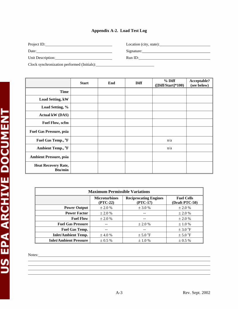
Appendix A-2. Load Test Log

Project ID: Location (city, state):

Date: Signature:

Unit Description: Run ID:

Clock synchronization performed (Initials):

Start End Diff % Diff ([Diff/Start]*100)

Acceptable? (see below)

Time

Load Setting, kW

Load Setting, %

Actual kW (DAS)

Fuel Flow, scfm

Fuel Gas Pressure, psia

Fuel Gas Temp., oF n/a

Ambient Temp., oF n/a

Ambient Pressure, psia

Heat Recovery Rate, Btu/min

Maximum Permissible Variations Microturbines

(PTC-22) Reciprocating Engines

(PTC-17) Fuel Cells

(Draft PTC-50) Power Output ± 2.0 % ± 3.0 % ± 2.0 % Power Factor ± 2.0 % ± 2.0 %

Fuel Flow ± 2.0 % ± 2.0 % Fuel Gas Pressure ± 2.0 % ± 1.0 %

Fuel Gas Temp. ± 3.0 oF Inlet/Ambient Temp. ± 4.0 % ± 5.0 oF ± 5.0 oF

Inlet/Ambient Pressure ± 0.5 % ± 1.0 % ± 0.5 %

Notes:

A-3 Rev. Sept. 2002

Appendix A-3. Fuel Gas Sampling Procedures

Important: Follow these procedures when the gas pressure is > 5 psi above atmospheric pressure.

1. For each day of emissions testing, collect at least one (1) gas sample immediately before starting the first test run and at least one (1) sample after the final test run of the day. During extended test periods, collect at least two (2) gas samples per week.

2. Attach a leak free vacuum gauge to the sample canister inlet. Open the canister inlet valve and verify that the canister vacuum is at least 15 “Hg. Record the gage pressure on the Fuel Sampling Log form.

3. Close the canister inlet valve, remove the vacuum gauge, and attach the canister to the fuel line sample port.

4. Open the fuel line sample port valve and check all connections for leaks with bubble solution or a hand held analyzer. Repair any leaks, then open the canister inlet valve. Wait firve (5) seconds to allow the canister to fill with fuel.

5. Open the canister outlet valve and purge the canister with fuel gas for at least five (5) but not more than eight (8) seconds. Close the canister outlet valve, canister inlet valve, and fuel line sampling port valve in that order.

6. Obtain the fuel gas pressure and temperature from the DAS display. Enter the required information (date, time, canister ID number, etc.) on the Fuel Sampling Log (Appendix A-4a) and Chain of Custody Record (Appendix A-5) forms. Remove the canister from the sampling port.

Important: Follow these procedures when the gas pressure is < 5 psi above atmospheric pressure.

1. Construct a leak free gas extraction and collection system such as shown in the following sketch.

Peristaltic Pump

Canister Evacuation Loop

Sample Canister

- Pressure/vacuum Gauge

- Flow Control Valves

Gas Purge Vent

2. Make a leak free connection from the gas source to the inlet of the gas collection system.

(continued)

A-4 Rev. Sept. 2002

Appendix A-3. Fuel Gas Sampling Procedures (continued)

3. Using the control valves and vacuum gauge, check and record the sample canister vacuum. If necessary, fully evacuate the canister using the peristaltic pump and control valves. Record the final canister vacuum (should be -25 in. Hg or less).

4. Isolate the evacuated canister and configure the valves so that gas is slowly vented through the purge vent (ensure proper ventilation of gas before starting the purge). Purge for 10 seconds.

5. Close the purge vent, and slowly open the valves upstream of the canister and allow the canister to pressurize to no less than 2 psig.

6. With the pump still running, open the canister outlet valve and purge the canister for 5 seconds. Sequentially close the canister outlet valve, canister inlet valve, and pump inlet valve. Turn off pump.

7. Record the date, time, gas temperature (from DAS), canister ID number, and final canister pressure on log form (Appendix A-4b).

8. Return collected sample(s) to laboratory with completed chain-of-custody form (Appendix A-5).

A-5 Rev. Sept. 2002

Appendix A-4. Fuel Sampling Log

Project ID:______________________ Location (city, state):___________________________________

Date:____________________ Signature:____________________________________________

Unit Description:_________________________ Fuel Source (pipeline, digester, etc.)________________

Note: If desired, assign random sample ID numbers to prevent the lab from attributing analysis results to a particular test or audit sample. Transfer sample ID numbers to Chain of Custody Record prior tosample shipment.

Obtain sample pressure and temperature from the DAS display.

Date Time Run ID Sample ID Canister ID Initial

Vacuum (“Hg)

Fuel Pressure

(DAS)

Fuel Temperature

(DAS)

Notes:

A-6 Rev. Sept. 2002

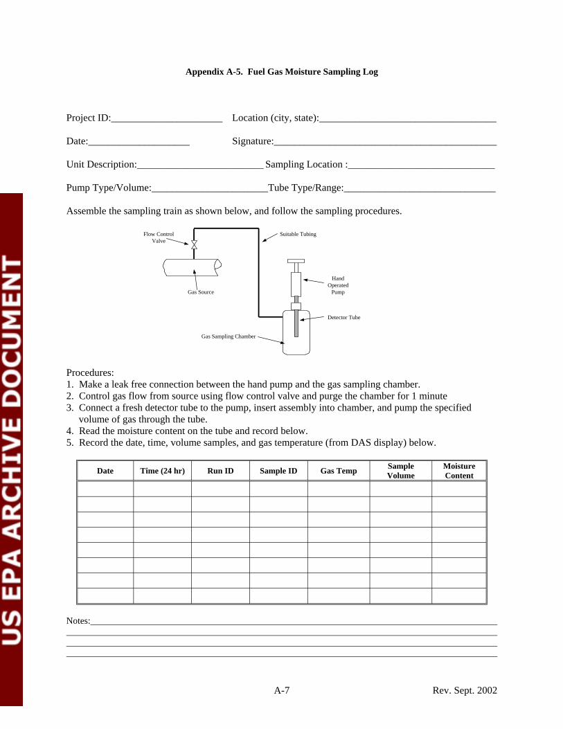
Appendix A-5. Fuel Gas Moisture Sampling Log

Project ID:______________________ Location (city, state):___________________________________

Date:____________________ Signature:____________________________________________

Unit Description:_________________________ Sampling Location :_____________________________

Pump Type/Volume:_______________________Tube Type/Range:______________________________

Assemble the sampling train as shown below, and follow the sampling procedures.

Pump

Suitable Tubing

Gas Sampling Chamber

Detector Tube

Hand Operated

Gas Source

Flow Control Valve

Procedures: 1. Make a leak free connection between the hand pump and the gas sampling chamber. 2. Control gas flow from source using flow control valve and purge the chamber for 1 minute 3. Connect a fresh detector tube to the pump, insert assembly into chamber, and pump the specified

volume of gas through the tube. 4. Read the moisture content on the tube and record below. 5. Record the date, time, volume samples, and gas temperature (from DAS display) below.

Date Time (24 hr) Run ID Sample ID Gas Temp Sample Volume

Moisture Content

Notes:

A-7 Rev. Sept. 2002

Appendix A-6. Example Chain-of-Custody Record

Southern Research Institute Chain-of-Custody Record

Important: Use separate Chain-of-Custody Record for each laboratory and/or sample type.

Project ID:

Originator’s signature:

Sample description & type (gas, liquid, other.):

Laboratory:

Address:

Location (city, state):

Unit description:

Phone: Fax:

City: State: Zip:

Sample ID Bottle/Canister ID Sample Pressure Sample Temp. (°F) Analyses Req’d

Relinquished by: Date: Time: Received by: Date: Time:

Relinquished by: Date: Time: Received by: Date: Time:

Relinquished by: Date: Time: Received by: Date: Time:

Notes: (shipper tracking #, other)

A-8 Rev. Sept. 2002

Appendix A-7. Gas Meter Transmitter Calibration Log

Project ID: Location (city, state):

Date: Signature:

1. Confirm stable fuel cell operations at full load. 2. Reading the meter's odometer type index, begin a calibration run by recording a start volume to the nearest

0.2 actual cubic feet (acf), and starting a stopwatch timer to record elapsed time (Secelapsed). Log the entries below.

3. After at least 100 acf of gas has been recorded on the meter index, take a final meter reading to the nearest 0.2 acf and stop the timer. Log the entries below and calculate gas flow rate (acfm).

4. Record the average gas flow rate (acfm) logged by the DAS during the test period. 5. Repeat the procedure two more times at full load. 6. Calculate the average difference between the meter index and the DAS readings. Log the entries below. 7. Repeat the entire procedure while operating the fuel cell at 75 and 50 percent of full load. 8. Record the DAS gas flow reading with the gas flow turned off (zero check).

Fuel Cell Power Setting (kW)

Run Number

Roots Meter Readings DAS Flow Rateb

(acfm) Differencec

(%) Start Time

Initial Reading

(acf) Stop Time

Final Reading

(acf)

Elapsed Time (sec.)

Flow Ratea

(acfm) 1

2

3

Avg

1

2

3

Avg

1

2

3

Avg

a Gas flow rate (acfm) = (final reading (acf) - initial reading (acf)) / elapsed time (sec.) * 60 b DAS gas flow rate (acfm) = average gas flow rate recorded by DAS during test run period a Difference (%) = (gas flow from meter (acfm) - gas flow from DAS (acfm)) / gas flow from meter (acfm) * 100

A-9 Rev. Sept. 2002

Appendix A-8. Heat Meter RTD QA Check

The heat meter receives temperature signals from two resistance temperature devices (RTDs), mounted upstream and downstream of the heat recovery unit. The data acquisition system (DAS) displays and records these temperatures. The GHG Center will evaluate the RTD performance by comparing the DAS displayed temperature values with a calibrated digital thermometer.

GHG Center personnel will conduct the performance check at least once prior to the start of testing as follows:

1. Simultaneously immerse the digital thermometer thermocouple and the RTDs under test. IMPORTANT: On direct contact RTDs, do not allow the top of the unit (with nameplate and electrical connector) to get wet.

2. While stirring, obtain the digital thermometer and DAS readings. Record below. 3. Repeat the procedure for hot water and ice baths. 4. Compare the RTD DAS readings to the digital thermometer readings. If differences exceed 1.5 oF,

the RTDs should be submitted for recalibration.

Project ID:_______________________________Location (city, state):___________________________

Date:________________ Signature:____________________________________________

Digital Thermometer Make:________________ Model:___________________ Serial No.___________

Thermocouple ID No.___________________ Last Calibration Date:_____________________

Performance Check Location (laboratory or field):______________

Heat Meter Make:_______________________ Model:___________________ Serial No.___________

RTD1 Model ____________ ID No.___________ Type (contact/immersion)___________

RTD2 Model ____________ ID No.___________ Type (contact/immersion)___________

Bath Description (hot/cool/ice)

RTD1 or RTD2?

RTD DAS Value

Digital Thermometer Value Difference Acceptable?

(<1.5 oF)

A-10 Rev. Sept. 2002

Appendix A-9. Heat Meter Setup and Reasonableness Check

Date: Unit:

Heat Meter Make: Model # Serial #:

Signature:

Enter the following values into the heat meter software:

Pipe Outside Diameter: Material: Wall Thickness:

Nom. Dia Schedule 40 Steel Pipe Type L Copper Tubing

Actual OD Wall Thickness Actual ID Actual OD Wall

Thickness Actual ID

1.25 1.660 0.140 1.380 1.375 0.055 1.265 1.50 1.900 0.145 1.610 1.625 0.060 1.505 2.00 2.375 0.154 2.067 2.125 0.070 1.985 2.50 2.875 0.203 2.469 2.625 0.080 2.465 3.00 3.500 0.216 3.068 3.125 0.090 2.945 3.50 4.000 0.226 3.548 3.625 0.100 3.425

Source: T. Baumeister, Ed. Standard Handbook for Mechanical Engineers, 7th Ed, McGraw Hill, NY, NY 1967

Acquire the following data from the DAS and perform the applicable calculations. Interpolate density and specific heat for Tavg from the reference table below or ASHRAE publications.

Date: Time (24-Hr):

DAS t1 ___________ tavg __________ t1-t2 _____________

DAS t2 ___________

DAS Gal/min ______ (Gal / min)

= ft 3 / min _____________4805.7

DAS Btu/min ______ Cp ______________ ρ _______________

Q = VρC p (t − t2 ) _______________1

Percent Difference: ( Btu DAS / min)−Q 100 * _____________

Q

Acceptable? (< 5 %) (Y/N) ______________

Reference -- Water Specific Heat and Density

Temp, oF ρ, lb/ft3 Cp, Btu/lb.oF Temp, oF ρ, lb/ft3 Cp,

Btu/lb.oF Temp, oF ρ, lb/ft3 Cp, Btu/lb.oF

100 61.9951 0.99799 140 61.3818 0.99943 180 60.5821 1.00272 110 61.8616 0.99817 150 61.1955 1.00008 190 60.3552 1.00388 120 61.7132 0.99847 160 61.0027 1.00082 200 60.1234 1.00517 130 61.5548 0.99889 170 60.7956 1.00172 210 59.8784 1.00388

Source: Interpolated from R. Weast, Ed., CRC Handbook, 60th Ed., CRC Press, Inc., Boca Raton, FL. 1979

A-11 Rev. Sept. 2002

Appendix A-10. 7600/7500 ION Installation and Setup Checks

Project ID: Location (city, state):

Date: Signature:

Unit Description:

IMPORTANT: Conformance to applicable local codes supercede the instructions in this log sheet or the 7600/7500 ION installation manual

Only qualified personnel shall install current transformers (CTs) or voltage transformers (PTs). To avoid risk of fire or shock, be sure that the CT shorting switch(es) are installed and operated properly.

Note: Instructions below pertain to both the 7600-ION and 7500-ION power meters. Initial each item upon completion.

_______ Obtain and read the ION Installation and Basic Setup Manual (manual). It is the source of the items outlined below and is the reference for further questions.

_______ Verify that the ION calibration certificate(s) and supporting data are on hand.

_______ Mount the meter(s) in a well-ventilated location free of moisture, oil, dust, and corrosive vapors. Ensure that all wiring conforms to NEC standards.

_______ Verify that the ION power source is 110 VAC, nominal, protected by a switch or circuit breaker. If used with the DAS, plug the meter into the DAS uninterruptable power supply (UPS).

_______ Connect each ION ground terminal (usually the “Vref” terminal) directly to the switchgear earth ground with a dedicated AWG 12 gauge wire or larger. In most 4-wire WYE setups, jumper the “V4” terminal to the “Vref” terminal. Refer to the manual for specific instructions.

_______ Choose the proper CTs and PTs for the application. Install them in the power circuit and connect them to the ION power meters according to the directions in the manual (pages 8-14).

_______ Trace or color code each CT and PT circuit to ensure that they go to the proper meter terminals. Each CT must match its corresponding PT (i.e. connect the CT for phase A to meter terminals I11 and I12 and connect the PT for phase A to meter terminals V1 and Vref).

_______ Use a digital volt meter (DVM) to measure each phase’s voltage and current. Enter the data on the ION Sensor Function Checks form and compare with the ION front panel.

_______ Confirm that the ION front panel readings agree with the DAS display.

_______ Compare the ION and DAS readings to the unit’s panel or controller display. Enter this information in the Daily Test Log as is appropriate.

_______ Verify that the DAS is properly logging and storing data by downloading data to the laptop computer and reviewing it.

(continued)

A-12 Rev. Sept. 2002

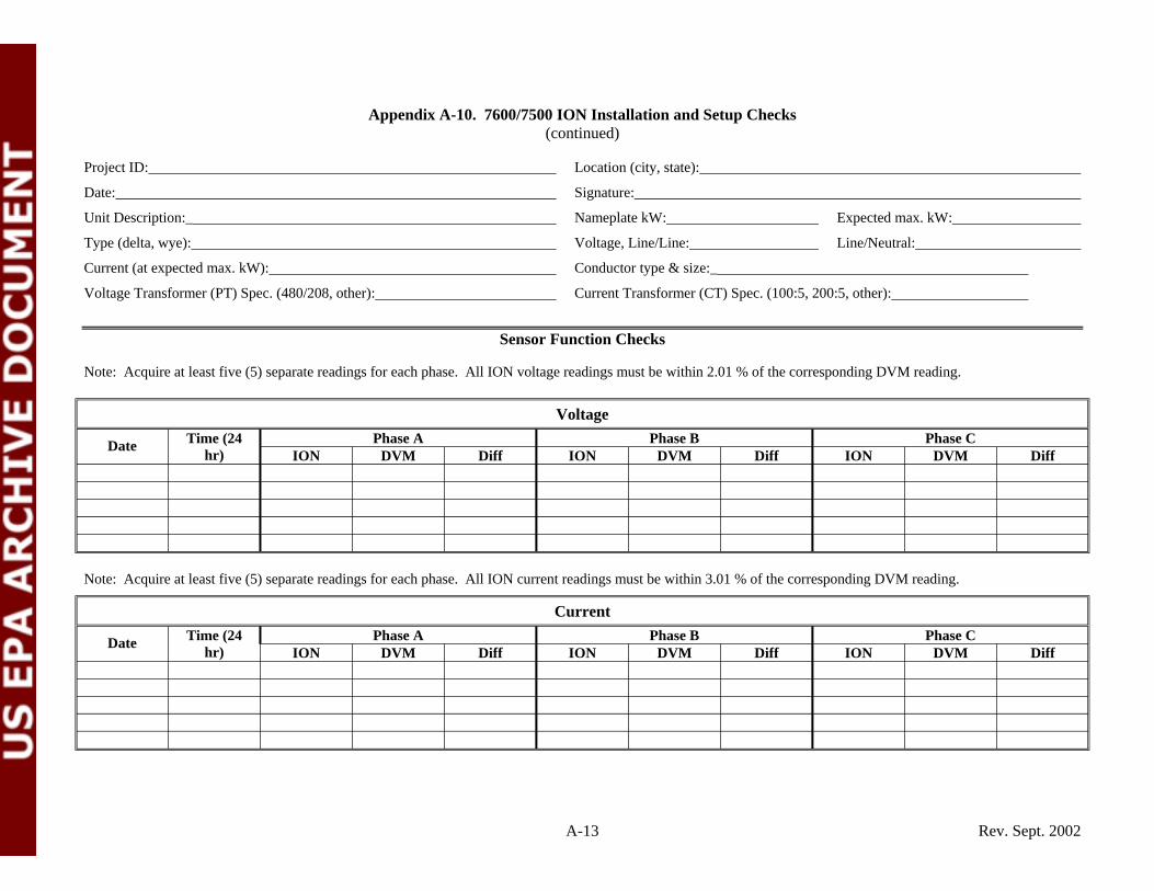
Appendix A-10. 7600/7500 ION Installation and Setup Checks (continued)

Project ID:

Date:

Unit Description:_

Type (delta, wye):

Current (at expected max. kW):

Voltage Transformer (PT) Spec. (480/208, other):

Location (city, state):

Signature:

Nameplate kW: Expected max. kW:

Voltage, Line/Line: Line/Neutral:

Conductor type & size:_

Current Transformer (CT) Spec. (100:5, 200:5, other):

Sensor Function Checks

Note: Acquire at least five (5) separate readings for each phase. All ION voltage readings must be within 2.01 % of the corresponding DVM reading.

Voltage

Date Time (24 hr)

Phase A Phase B Phase C ION DVM Diff ION DVM Diff ION DVM Diff

Note: Acquire at least five (5) separate readings for each phase. All ION current readings must be within 3.01 % of the corresponding DVM reading.

Current

Date Time (24 hr)

Phase A Phase B Phase C ION DVM Diff ION DVM Diff ION DVM Diff

A-13 Rev. Sept. 2002

Appendix A-11. ION Sensor Function Checks

Date: Project:

QA/QC Test Leader Name:

Phase Wiring (Delta or Wye):

Initial all items after they have been completed.

_____ 7600 ION calibration certificates and supporting data are on-hand.

_____ Check power supply voltage with a DMM (should be between 85 and 240 VAC.)

_____ Check the 7600 ION ground terminal connection for continuity with the switchgear earth ground.

_____ Use a digital multimeter (DMM) to check that the phase and polarity of the AC voltage inputs are correct.

_____ Verify the operation of the 7600 ION according to the instructions in the 7600 ION INSTALLATION & BASIC SETUP MANUAL [page 30].

_____ Using a DMM measure the voltage and current for each phase and compare them to the readings on the display of the 7600 ION. The readings on the DMM should agree (within the tolerance of the meters) with the readings from the 7600 ION.

_____ Confirm that the readings on the 7600 ION agree with the corresponding readings on the DAS. If they do not agree, troubleshoot the communications link until proper readings are obtained by the DAS.

_____ Verify that the readings are being properly stored on the DAS hard disk or other non-volatile memory.

Load %

24-hr Time

Voltage, V Current, Amps

Phase A Phase B Phase C Phase A Phase B Phase C 7600 ION DVM 7600

ION DVM 7600 ION DVM 7600

ION DVM 7600 ION DVM 7600

ION DVM

Average

% Diff = [(ION-DVM) / ION] * 100

A-14 Rev. Sept. 2002

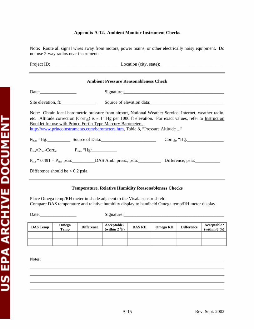
Appendix A-12. Ambient Monitor Instrument Checks

Note: Route all signal wires away from motors, power mains, or other electrically noisy equipment. Do not use 2-way radios near instruments.

Project ID:_______________________________Location (city, state):___________________________

Ambient Pressure Reasonableness Check

Date:________________ Signature:____________________________________________

Site elevation, ft:_______________ Source of elevation data:________________________________

Note: Obtain local barometric pressure from airport, National Weather Service, Internet, weather radio, etc. Altitude correction (Corralt) is ≈ 1” Hg per 1000 ft elevation. For exact values, refer to Instruction Booklet for use with Princo Fortin Type Mercury Barometers, http://www.princoinstruments.com/barometers.htm, Table 8, “Pressure Altitude ...”

Pbar, “Hg:__________ Source of Data:________________________ Corralt, “Hg:________________

Psta=Pbar-Corralt Psta, “Hg:___________

Psta * 0.491 = Psta, psia:__________DAS Amb. press., psia:__________ Difference, psia:___________

Difference should be < 0.2 psia.

Temperature, Relative Humidity Reasonableness Checks

Place Omega temp/RH meter in shade adjacent to the Visala sensor shield. Compare DAS temperature and relative humidity display to handheld Omega temp/RH meter display.

Date:________________ Signature:____________________________________________

DAS Temp Omega Temp Difference Acceptable?

(within 2 oF) DAS RH Omega RH Difference Acceptable? (within 8 %)

Notes:

A-15 Rev. Sept. 2002

Appendix A-13. Corrective Action Report

Corrective Action Report

Verification Title:

Verification Description:

Description of Problem:

Originator: Date:

Investigation and Results:

Investigator: Date:

Corrective Action Taken:

Originator: Date: Approver: Date:

Carbon copy: GHG Center Project Manager, GHG Center Director, SRI QA Manager, APPCD Project Officer

A-16 Rev. Sept. 2002

A-17 Rev. Sept. 2002