DAHLGREN DIVISION NAVAL SURFACE WARFARE CENTER Dahlgren, Virginia 22448-5100

NSWCDD/TR-12/68

SOFTWARE USER’S MANUAL FOR THE RAILCAR4 TOXIC INDUSTRIAL CHEMICAL SOURCE CHARACTERIZATION PROGRAM BY TIMOTHY J. BAUER

ASYMMETRIC SYSTEMS DEPARTMENT AUGUST 2011 Approved for public release; distribution is unlimited.

NSWCDD/TR-12/68

i/ii

REPORT DOCUMENTATION PAGE Form Approved OMB No. 0704-0188

Public reporting burden for this collection of information is estimated to average 1 hour per response, including the time for reviewing instructions, search existing data sources, gathering and

maintaining the data needed, and completing and reviewing the collection of information. Send comments regarding this burden or any other aspect of this collection of information, including

suggestions for reducing this burden, to Washington Headquarters Services. Directorate for information Operations and Reports, 1215 Jefferson Davis Highway, Suite 1204, Arlington, VA 22202-4302,

and to the Office of Management and Budget, Paperwork Reduction Project (0704-0188), Washington, DC 20503.

1. AGENCY USE ONLY (Leave blank) 2. REPORT DATE

August 2011

3. REPORT TYPE AND DATES COVERED

Final

4. TITLE AND SUBTITLE

SOFTWARE USER’S MANUAL FOR THE RAILCAR4 TOXIC INDUSTRIAL CHEMICAL SOURCE CHARACTERIZATION PROGRAM

5. FUNDING NUMBERS

6. AUTHOR(s) Timothy J. Bauer

7. PERFORMING ORGANIZATION NAME(S) AND ADDRESS(ES) Naval Surface Warfare Center, Dahlgren Division CBR Analysis, Testing, & Systems Engineering Branch (Code Z24) 4045 Higley Road, Suite 344 Dahlgren, VA 22448-5162

8. PERFORMING ORGANIZATION REPORT NUMBER

NSWCDD/TR-12/68

9. SPONSORING/MONITORING AGENCY NAME(S) AND ADDRESS(ES) 10. SPONSORING/MONITORING AGENCY REPORT NUMBER

11. SUPPLEMENTARY NOTES

12a. DISTRIBUTION/AVAILABILITY STATEMENT

Approved for public release; distribution is unlimited.

12b. DISTRIBUTION CODE

13. ABSTRACT (Maximum 200 words)

This document discusses the use of the RAILCAR4 Toxic Industrial Chemical Source Characterization Program to analyze a scenario in which there is a release of a toxic industrial chemical from a transport tank, such as chlorine released from a rupture in a 90-ton railcar. Knowledge gaps associated with such a release are discussed, the most important of which fall into three categories: 1) characterization of the vapor source resulting from the liquid jet, 2) human toxic effects, and 3) reaction of the chlorine vapor with and removal by surfaces and air as it travels downwind. The RAILCAR4 Program addresses the first of these knowledge gaps.

The study concludes that, as a result of the validation of the Naval Surface Warfare Center, Dahlgren Division (NSWCDD) mist pool theory, in conjunction with extensive measurements taken during Jack Rabbit pilot tests and field trials, hazard assessment models will be better equipped to predict downwind effects for emergency responders, and warfighters will be much better protected from these types of attacks.

14. SUBJECT TERMS toxic industrial chemical, TIC, RAILCAR program, mist pool theory, vapor plume formation, downwind effects, hazard assessment models

15. NUMBER OF PAGES 68

16. PRICE CODE

17. SECURITY CLASSIFICATION OF REPORTS

UNCLASSIFIED

18. SECURITY CLASSIFICATION OF THIS PAGE

UNCLASSIFIED

19. SECURITY CLASSIFICATION OF ABSTRACT

UNCLASSIFIED

20. LIMITATION OF ABSTRACT

UL

NSN 7540-01-280-5500 Standard Form 298 (Rev 2-89) Prescribed by ANSI std. Z39-18 298-102

NSWCDD/TR-12/68

iii/iv

FOREWORD This document discusses the use of the RAILCAR4 Toxic Industrial Chemical Source Characterization Program to analyze a scenario in which there is a release of a toxic industrial chemical from a transport tank, such as chlorine released from a rupture in a 90-ton railcar. Knowledge gaps associated with such a release are discussed, the most important of which fall into three categories: 1) characterization of the vapor source resulting from the liquid jet, 2) human toxic effects, and 3) reaction of the chlorine vapor with and removal by surfaces and air as it travels downwind. The RAILCAR4 Program addresses the first of these knowledge gaps. The study concludes that, as a result of the validation of the Naval Surface Warfare Center, Dahlgren Division (NSWCDD) mist pool theory, in conjunction with extensive measurements taken during Jack Rabbit pilot tests and field trials, hazard assessment models will be better equipped to predict downwind effects for emergency responders, and warfighters will be much better protected from these types of attacks.

This report has been reviewed by Gaurang R. Davë, Head, CBR Analysis, Testing, & Systems Engineering Branch (Code Z24), and Michael Purello, Head, CBR Defense Division. Approved by:

JOHN LYSHER, Head Asymmetric Systems Department

NSWCDD/TR-12/68

v

CONTENTS Section Page

1.0 INTRODUCTION ................................................................................................1

1.1 Vapor Source Characterization .....................................................................2

1.2 Human Toxic Effects .....................................................................................3

1.3 Reaction and Removal Mechanisms .............................................................4

2.0 RAILCAR PROGRAM DEVELOPMENT ..........................................................6

2.1 RAILCAR Studies and Analyses ..................................................................8

2.2 The RAILCAR Validation Issue ...................................................................9

2.3 Jack Rabbit Test Program ............................................................................10

2.4 New Algorithm Development and Adjustment ...........................................12

2.5 Comparison with Jack Rabbit Data .............................................................14

2.6 RAILCAR4 Development ...........................................................................18

3.0 RAILCAR4 OPERATOR’S INSTRUCTIONS .................................................22

3.1 TIC Thermodynamic Property Files ............................................................22

3.2 Input Parameters and Algorithms ................................................................23

3.3 Wind Condition Input ..................................................................................29

3.4 Executing the Program ................................................................................31

3.5 Interpreting the Output File .........................................................................32

3.6 Operation as a Subroutine ...........................................................................43

3.7 Subroutine Structure and Function ..............................................................47

4.0 CONCLUSIONS.................................................................................................51

5.0 REFERENCES ...................................................................................................52

DISTRIBUTION................................................................................................ (1)

NSWCDD/TR-12/68

vi

ILLUSTRATIONS Figure Page

1 TIC Vapor Plume Formation Versus Pooling at the Release Site ...........................3

2 Hypothetical TIC Incident Common Casualty Estimation Approaches ..................5

3 Hypothetical TIC Incident Toxic Load Casualty Estimation Approach ..................5

4 Jack Rabbit Test Design.........................................................................................10

5 Jack Rabbit Ammonia and Chlorine Video Images ...............................................11

6 Comparison of RAILCAR3 Predictions with Data for Ammonia Trial 04-RA ....16

7 Comparison of RAILCAR3 Predictions with Data for Chlorine Trial 05-RC ......17

8 RAILCAR4 Predictions for Ammonia Trial 04-RA ..............................................20

9 RAILCAR4 Predictions with Data for Chlorine Trial 05-RC ...............................20

10 Nitric Acid Thermodynamic Properties .................................................................23

11 RAILCAR TIC List ...............................................................................................31

12 Example RAILCAR.DAT File ..............................................................................32

13 RAILCALC Subroutine Call .................................................................................44

14 RAILCALC Input and Output Parameter Declarations .........................................44

NSWCDD/TR-12/68

vii

TABLES Table Page

1 TICs Available for RAILCAR Simulations .............................................................9

2 RAILCAR3 Prediction Errors for Tank and Jet Properties ...................................17

3 RAILCAR3 Prediction Errors for Stationary Cloud and Liquid Pool Properties ..18

4 RAILCAR4 Prediction Errors................................................................................21

5 RAILCALC Parameter Definitions .......................................................................45

NSWCDD/TR-12/68

viii

GLOSSARY AEGL Acute Exposure Guideline Level CSAC Chemical Security Analysis Center (DHS) CSG Challenge Sub-Group DHS Department of Homeland Security DoD Department of Defense DPG Dugway Proving Ground FFI Norwegian Defense Research Establishment JECP Joint Expeditionary Collective Protection NATO North Atlantic Treaty Organization NSWCDD Naval Surface Warfare Center, Dahlgren Division OHA Operational Hazard Analysis SME Subject Matter Expert S&T Science and Technology TIC Toxic Industrial Chemical TIM Toxic Industrial Material TSA Transportation Security Administration VLSTRACK (Chemical and Biological Agent) Vapor, Liquid, and Solid Tracking

NSWCDD/TR-12/68

1

1.0 INTRODUCTION

On January 6, 2005, a train wreck in Graniteville, South Carolina, led to the rupture of a 90-ton chlorine railcar resulting in the release of 54 tons of chlorine.1 Over 5000 people in the lightly populated area were evacuated; over 500 people sought medical treatment; 9 people died. This accident led to concern among city planners, emergency responders, the transportation industry, the chemical industry, the Department of Homeland Security (DHS), and the Department of Defense (DoD) about potential attacks on chemical railcars and tanker trucks transiting an urban area, or chemical storage tanks near an urban area. A comparison of modern hazard assessment model predictions at the time consistently suggested that lethal concentrations from large releases of chlorine would persist within the plume of toxic vapor beyond six miles downwind.2 Modeling results indicated that hundreds of thousands of persons would need to be evacuated as the plume spread rapidly through the urban area.

Such a large evacuation effort would be impractical for emergency responders in terms of both resources and time. Further, records of toxic effects from accidents like that in Graniteville suggest the downwind hazard area is much shorter than the hazard assessment models predict. The nine deaths in Graniteville all occurred within half a mile of the accident. The World War I Battle of Ypres, France, on 22 April 1915 involved release of chlorine from several thousand cylinders along a four mile-long trench, but deaths were limited to within less than one half mile of the release trench.3 Even the over 2,000 deaths in Bhopal, India that resulted from the December 3, 1984 release of 40 tons of methyl isocyanate occurred within less than two miles; the large number of deaths were associated with the high population density rather than the downwind distance of that highly toxic chemical.4

To address the large discrepancy between recorded toxic effects and model predictions, the Transportation Security Administration (TSA) assembled a group of subject matter experts (SMEs) from the chemical industry, transportation industry, national labs, academia, emergency response organizations, DHS, DoD, and the intelligence community. A meeting was held on November 8-9, 2006 in McLean, Virginia, and was co-chaired by this document’s author from the Naval Surface Warfare Center Dahlgren Division (NSWCDD).5 Discussions focused on the release of chlorine from a 90-ton railcar and the identification of knowledge gaps associated with such a release. The most important knowledge gaps fell into three categories: 1) characterization of the vapor source resulting from the liquid jet, 2) human toxic effects, and 3) reaction of the chlorine vapor with and removal by surfaces and air as it travels downwind. Each is discussed below.

NSWCDD/TR-12/68

2

1.1 Vapor Source Characterization

Survivors of the Graniteville accident reported that chlorine vapor remained in the release area for at least two hours. The chlorine vapor plume also followed the path of the valley within which Graniteville is located, which was somewhat different from the wind direction at the time of the accident. The chlorine was thus heavily influenced by the terrain features, along with the buildings and vegetation in the release area. Conversely, hazard prediction models all assumed that the liquid jet would mix with passing air and be carried downwind as a long vapor plume. These modeling approaches agreed with data from field trials involving large releases of toxic industrial chemicals (TICs), such as ammonia; but those releases occurred over flat desert terrain under a fairly high wind speed. Field trials were limited by available test sites and the requirement that the wind direction remain steady and predictable for safety reasons.6

One theory addressing these additional features, developed by the author in 2008, was that large TIC masses of vapor and aerosol released over a short time period would pool into a large cloud at the release site and give off vapor into the passing air over an extended time period.7 This pooling was likely enhanced by the presence of buildings, vegetation, and terrain depressions in the release area. The significance of having a long duration source of vapor instead of a short duration plume was that the concentration of the chemical downwind of the release site was lower and less toxic, especially when coupled with the human toxic effects described in the next section. TIC vapor plume formation versus pooling at the release site is shown in Figure 1.

NSWCDD/TR-12/68

3

Figure 1. TIC Vapor Plume Formation Versus Pooling at the Release Site 1.2 Human Toxic Effects

The model predictions used to estimate the downwind hazard areas were based on chemical concentrations called Acute Exposure Guideline Levels (AEGLs) developed for the Environmental Protection Agency.8 For a given chemical, there are AEGLs for life-threatening, serious, and irritating effects. Human toxic responses are a function of exposure (which combines concentration and duration), rather than just concentration, so there are AEGLs for a range of exposure durations ranging from 10 minutes to 8 hours. The problem with the AEGLs identified by the SMEs was that they were set for the most sensitive subpopulation rather than the average person. Thus, the AEGLs cannot be used to estimate expected casualties from a TIC incident.

An important aspect of human toxic responses is that, for one-time acute exposures, the human body can slowly expel or otherwise counter a toxic chemical. A high concentration received over a short duration, therefore, is more toxic than an equivalent exposure involving a low concentration over a longer time period. This “toxic load” approach reveals why lowering the vapor concentration at the release location, as discussed above, can dramatically reduce the

NSWCDD/TR-12/68

4

size and length of the downwind hazard area. Even if the TIC does travel downwind as a high concentration plume, use of higher toxicity values appropriate for the average person and the toxic load approach with existing hazard prediction models will greatly improve model output.

The importance of proper source characterization and toxicity estimation can be demonstrated using a hypothetical scenario involving release of a TIC. Figure 2 shows the number of persons requiring medical attention (i.e., casualties) using three common hazard area representations: circle, fan, and contour. The population density is assumed uniform, so casualties reflect relative areas within each representation. The radius of the circle and fan and the length of the contour are the same and represent the current AEGL approach. Casualties ranged from 1288 within the model contour to 22,182 if a simple circle is drawn. If the toxic load approach is then used with the same model output but using toxicity values for the total population distribution (as opposed to the most sensitive subpopulation), the length of the contour decreases considerably, and the number of casualties drops to 32, as shown in Figure 3. 1.3 Reaction and Removal Mechanisms

Reaction of the TIC vapor with surface materials such as concrete and metal, reaction with water vapor and air pollutants, and absorption into the surface materials at the release location all act to decrease the TIC mass traveling downwind, resulting in lower concentrations and reduced downwind toxic effects. The chlorine vapor at Graniteville penetrated the ground at the release site and had to be neutralized with large amounts of lime. As the chlorine vapor traveled downwind, it corroded exposed metal surfaces such as doorknobs and electrical transformers. The vapor reaction with surface materials formed a different compound, pulling mass out of the vapor plume and lowering its concentration. Chlorine vapor was also absorbed into porous materials such as building insulation. One issue with absorption is that, once the plume has moved on, the TIC may then desorb from within the surface. This process would result in a low concentration over an extended time period and reduced toxic effects, but not a lower total vapor mass. Although some TIC reaction data exists, the data were generated for pollution monitoring purposes using very low TIC concentrations rather than the high concentrations relevant to incidents. Data are still needed on how fast and how far the relevant reactions will occur to estimate the mass removed from the plume as it travels downwind.

NSWCDD/TR-12/68

5

Figure 2. Hypothetical TIC Incident Common Casualty Estimation Approaches

Figure 3. Hypothetical TIC Incident Toxic Load Casualty Estimation Approach

22,182 casualties3697 casualties 1288 casualties

32 casualties

NSWCDD/TR-12/68

6

2.0 RAILCAR PROGRAM DEVELOPMENT

The mist pool theory published by Bauer and Fox through the DHS Chemical Security Analysis Center (CSAC) is:7

Under low to moderate wind speeds, if the mass flow of a pressurized liquid jet exceeds the capacity of the passing air to entrain it, the vapor and aerosol will form a stationary cloud or “mist pool” at the release location and result in an area source vapor flux; mist pool behavior is enhanced by the presence of buildings, vegetation, and terrain depressions.

The significance of having a mist pool form in place of a plume from the two-phase jet is that the lower vapor concentrations, when combined with toxic load values, lead to greatly reduced downwind hazard distances that are consistent with incident observations.

Bauer and Fox define a single criterion to determine if a mist pool will form:

Qv /Q = 2.87 B C u* Dc2/(8 Q Ri* ) < 1 [1]

Dc = [4 Q (1 + E ρair/ ρJ)/ ρc Hc]

0.5 t0.5 [2]

Ri* = g (ρc – ρair) Hc/ ρair u*

2 [3]

where Qv is the vapor mass entrainment rate, Q is the jet mass flow rate, C is the mist pool concentration, u* is the friction velocity for the ambient wind conditions, is the constant pi, Dc is the mist pool diameter, Ri* is the friction-velocity-based Richardson number, E is the volumetric air entrainment ratio equal to the volume of air mixed into the jet over the volume of the jet, air is the ambient air density, J is the jet density, c is the mist pool density after air entrainment, Hc is the mist pool height or thickness, t is the tank empty time, and g is the gravitational acceleration constant (9.81 m/s2). B is an entrainment factor set to 5 if entrainment is enhanced by the jet aiming upwards or with the wind or the terrain is flat and smooth, as was typical for the desert field trials mentioned above. B is set to 0.2 if entrainment is inhibited by the presence of buildings, vegetation, and/or terrain undulations at the release location that shelter the jet from the ambient wind. B is set to 1 if entrainment is neither enhanced nor sheltered.

In order to estimate the vapor mass entrainment rate, a mist pool must be assumed to form using the TIC mass released in the jet. Jet mass flow rate and tank empty time are computed from the size of the hole in the tank and calculations of the thermodynamic behavior

NSWCDD/TR-12/68

7

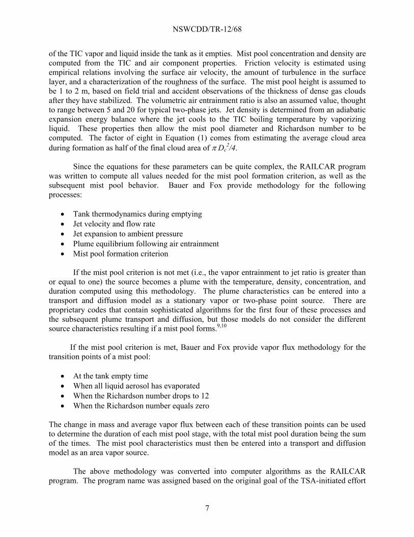
of the TIC vapor and liquid inside the tank as it empties. Mist pool concentration and density are computed from the TIC and air component properties. Friction velocity is estimated using empirical relations involving the surface air velocity, the amount of turbulence in the surface layer, and a characterization of the roughness of the surface. The mist pool height is assumed to be 1 to 2 m, based on field trial and accident observations of the thickness of dense gas clouds after they have stabilized. The volumetric air entrainment ratio is also an assumed value, thought to range between 5 and 20 for typical two-phase jets. Jet density is determined from an adiabatic expansion energy balance where the jet cools to the TIC boiling temperature by vaporizing liquid. These properties then allow the mist pool diameter and Richardson number to be computed. The factor of eight in Equation (1) comes from estimating the average cloud area during formation as half of the final cloud area of Dc

2/4.

Since the equations for these parameters can be quite complex, the RAILCAR program was written to compute all values needed for the mist pool formation criterion, as well as the subsequent mist pool behavior. Bauer and Fox provide methodology for the following processes:

Tank thermodynamics during emptying Jet velocity and flow rate Jet expansion to ambient pressure Plume equilibrium following air entrainment Mist pool formation criterion

If the mist pool criterion is not met (i.e., the vapor entrainment to jet ratio is greater than

or equal to one) the source becomes a plume with the temperature, density, concentration, and duration computed using this methodology. The plume characteristics can be entered into a transport and diffusion model as a stationary vapor or two-phase point source. There are proprietary codes that contain sophisticated algorithms for the first four of these processes and the subsequent plume transport and diffusion, but those models do not consider the different source characteristics resulting if a mist pool forms.9,10

If the mist pool criterion is met, Bauer and Fox provide vapor flux methodology for the transition points of a mist pool:

At the tank empty time When all liquid aerosol has evaporated When the Richardson number drops to 12 When the Richardson number equals zero

The change in mass and average vapor flux between each of these transition points can be used to determine the duration of each mist pool stage, with the total mist pool duration being the sum of the times. The mist pool characteristics must then be entered into a transport and diffusion model as an area vapor source.

The above methodology was converted into computer algorithms as the RAILCAR program. The program name was assigned based on the original goal of the TSA-initiated effort

NSWCDD/TR-12/68

8

to estimate the source conditions and subsequent transport and diffusion of chlorine released from a 90-ton railcar. RAILCAR originally only contained thermodynamic properties for chlorine and was limited to chlorine railcar, transport truck, and 1-ton shipping tanks. The thermodynamic properties of anhydrous ammonia were then added to allow for comparison of these two most commonly shipped TICs. RAILCAR does not compute TIC transport and diffusion. 2.1 RAILCAR Studies and Analyses

Multiple DoD, DHS, and international organizations are interested in estimating the toxic hazard areas resulting from TIC incidents. The Toxic Industrial Chemical/Toxic Industrial Material (TIC/TIM) Task Force was established by the Joint Program Executive Office for Chemical and Biological Defense in 2007 to develop a prioritized list of TICs. The Task Force determined the relative ranking of over 400 TICs and arrived at a list containing the highest ranked chemicals, which was further reduced to 16 priority TICs.11 The toxicity, volatility, and shipping quantities of these TICs led to their rankings, but it was still to be determined if they could be released in a manner leading to a large downwind inhalation/ocular hazard area.

DHS CSAC developed a similar list of TICs of concern for homeland security. The ones relevant to inhalation toxicity overlapped considerably with the DoD list. DHS Science and Technology (S&T) directorate funding allowed thermodynamic properties of 42 chemicals to be added to chlorine and ammonia in RAILCAR.12 Thirty-nine of the 44 total chemicals are the highest ranking ones from the TIC/TIM Task Force and include chlorine and anhydrous ammonia. The remaining chemicals are:

Acrolein—considered a priority TIC by the North Atlantic Treaty Organization (NATO) Challenge Sub-Group (CSG)

Ethylene Oxide—of TSA and industry concern as both a toxic and explosive downwind hazard

1,1,1,2-tetrafluoroethane (R134)—a refrigerant having potential as a chlorine and ammonia simulant

Dichloromethane—an organic solvent for pesticide dispersal Water—a solvent for TICs in aqueous solution (e.g., ammonium hydroxide, hydrofluoric

acid) The list of TICs for which thermodynamic properties are available for RAILCAR is included in Table 1.

The DHS S&T task also allowed for additional RAILCAR algorithm development to address processes associated with TICs having lower volatility, such as liquid pool evaporation. Again, other models contain similar algorithms, but RAILCAR is the only program that combines these source characterizations in a single model.

RAILCAR was used as part of a TIC/TIM Task Force operational hazard analysis (OHA) to provide source characterization for vignettes to determine the potential hazard of these TICs if

NSWCDD/TR-12/68

9

released in an attack against forward deployed troops.13 RAILCAR has also been used for a second OHA that addresses limitations identified with the first OHA and includes vignettes for additional priority TICs. RAILCAR was used to estimate the source characteristics for six chlorine vignettes and one acrolein vignette for a NATO CSG study that provides concentration challenge levels to NATO protective equipment.14 The program was used in a study for the Joint Expeditionary Collective Protection (JECP) acquisition program to characterize the sources for chlorine and sulfur dioxide vignettes for evaluating JECP shelter performance for proposed designs.15 RAILCAR was also used to characterize the source for the TSA for potential chlorine and ethylene oxide railcar attacks in urban areas and as part of a Navy shipboard threat study involving attacks on Navy ships in port using six different TICs.

Table 1. TICs Available for RAILCAR Simulations

chlorine hydrobromic acid (48%) acetylene tetrabromide ammonia OMPA o-anisidine ammonium hydroxide (29%) boron trifluoride sulfur trioxide hydrogen chloride methyl bromide phosphine hydrochloric acid (39%) phosphoryl trichloride arsine sulfuric acid chlorine dioxide ethylene dibromide hydrogen fluoride bromine 1,1,2,2-tetrachloroethane hydrofluoric acid (38%) nitrogen dioxide hydrogen cyanide formaldehyde phosphorus trichloride cyanogen chloride Formalin (37%) fluorotrichloromethane dichloromethane mercury hydrogen sulfide water nitric acid toluene-2,4-diisocyanate 1,1,1,2-tetrafluoroethane sulfur dioxide fluorine acrolein phosgene malathion ethylene oxide hydrogen bromide parathion

2.2 The RAILCAR Validation Issue

The mist pool theory, as defined in the Bauer and Fox report, was reviewed by members of the TSA group of SMEs prior to publishing. CSAC also funded external reviews. The theory was found credible; however, at the time there were no data involving formation of a mist pool from release of a pressurized liquid. What did exist were observations from accidents and attacks. Observers of the Graniteville accident reported patches of chlorine hanging around the release location for at least two hours.1 Some of the chlorine from the Ypres cylinders settled into the downwind trenches where it remained well beyond when the bulk of the plumes had dissipated.3 The chlorine transfer line rupture in Festus, Missouri was near a row of trees that effectively prevented chlorine from passing to the other side.16 In addition, field trials, wind tunnel, and water chamber tests involving releases of denser-than-air (or denser-than-water) materials under very low flow conditions were identified by the TSA SMEs, which showed

NSWCDD/TR-12/68

10

stationary cloud formation and/or detrainment of mass into the air/water flow above. The vapor mass entrainment rate equations, in Section 2 above, were selected from three sources that had already proposed algorithms dealing with creation of a stationary vapor cloud above a boiling liquid pool.17-20

Since none of the trials involved formation of a mist pool under more moderate wind speeds from release of a pressurized liquid, comparison of the RAILCAR mist pool methodology to data could only involve showing that the test conditions did not meet the mist pool formation criterion. The ammonia releases of the Desert Tortoise field trials do not meet the criterion.21 The U.S. Army conducted the Wild Stallion field trials at Dugway Proving Ground (DPG) releasing chlorine from 1-ton tanks in October 2007;22 these tests were conducted in response to the attacks in Iraq employing similar 1-ton chlorine tanks.23 Although, parts of the resulting chlorine clouds and plumes did remain at the release location for up to 30 seconds, RAILCAR predicts a much longer mist pool duration. In order to validate both the mist pool theory and the RAILCAR program, new data are needed. 2.3 Jack Rabbit Test Program

The most significant effort to date to generate data necessary to improve downwind hazard area estimation was the set of field trials conducted at DPG during the period 27 April through 21 May 2010. Pilot tests of ammonia and chlorine releases were conducted on 7 April and 8 April, respectively. Funding was provided by TSA and managed by ECBC; the project was operated by CSAC, and the trials were conducted by DPG.24 The test design (Figure 4) was created by NSWCDD and the Norwegian Defense Research Establishment (FFI).

Figure 4. Jack Rabbit Test Design

NSWCDD and FFI took advantage of an existing collaborative effort to work on the Jack Rabbit Test Program. The field trials were intended to prove or disprove the NSWCDD theory regarding the pooling of chlorine (or other TICs transported as pressurized liquids) vapor and aerosol at the release location, so the design included a circular pit designed to shelter chlorine and ammonia against the wind flowing over it. The goal was to have a tank empty time of

NSWCDD/TR-12/68

11

30 seconds and mist pool duration of 5 min. RAILCAR and other jet models were used to determine the hole, pipe, and valve sizes. RAILCAR projected that a wind speed of 2 to 3 m/s under stable conditions or 1 to 2 m/s under neutral conditions would result in the 5-min mist pool duration. The test geometry was refined by FFI using computational fluid dynamics modeling.25 Instrumentation was specified and positioned by the TSA group of SMEs. Four trials each were conducted with chlorine and ammonia involving the rapid release of two tons of liquid directed downward into the pit. The same tanks were used for the two pilot tests, but the tanks were only filled with one ton of each TIC. NSWCDD and FFI provided on-site modeling and analysis support during the trials. The trials did result in chlorine and ammonia pooling in the pit and releasing vapor into the passing air, validating the mist pool theory (see Figure 5). As described below, however, additional algorithms had to be developed and added to RAILCAR to be able to simulate the ammonia and chlorine behavior. By adjusting several input parameters, good agreement with data was obtained; however, as the Jack Rabbit field trial data were used to adjust the model, additional field trials are now needed to validate the program.

Figure 5. Jack Rabbit Ammonia and Chlorine Video Images (extracted from DPG videos)

Ammonia Pilot Test at <10 sec

Ammonia Pilot Test at 3 min

Chlorine Pilot Test at <10 sec

Chlorine Pilot Test at 3 min

NSWCDD/TR-12/68

12

2.4 New Algorithm Development and Adjustment

The methodology defined by Bauer and Fox and coded as the original RAILCAR program was insufficient to simulate the ammonia and chlorine Jack Rabbit field trials. New algorithms were developed and existing ones adjusted during the trial period. The resulting RAILCAR2 program was able to match key parameters measured during the field trials. The rapid code changes, though, made the source code quite unstructured. The source code was rewritten in a modular fashion after completion of the test program. The algorithms and their operation were verified by the author. The result was the RAILCAR3 program.

The tanks had three characteristics not addressed by the mist pool theory methodology. First, the mist pool theory assumed the tank to be completely full of liquid. Real transport and storage tanks, and the Jack Rabbit tanks after filling, have a vapor space above the liquid called ullage. The initial tank conditions, therefore, have both liquid and vapor present. Second, the air in the empty tanks is displaced to some extent during the filling process, but much of the air is trapped and compressed into the ullage volume. Industry will also add nitrogen to pressure tanks to make sure rupture disks and relief valves are within their proper pressure range. Third, SME concerns over vaporization within the pipes and values attached to the tank bottom led to restrictor orifices being constructed. A vapor phase was added to the algorithms for initial tank conditions, which had to be carried through the tank emptying algorithms. An inert vapor phase was likewise added to the same set of algorithms. The jet mass flow algorithms were modified by adding the area ratio of the orifice to the inner pipe/valve and assuming no additional frictional losses. The RAILCAR program also had a lower limit of 0 °C for the tank and air temperatures and had to be lowered for the test conditions.

Once the pilot tests and field trials began, a series of “significant observations” required additional RAILCAR algorithm development and modifications. The most significant of these observations was that the volumetric air entrainment ratio was much higher than the assumed range of 5 to 20. Based on the final cloud diameter and thickness and the measured cloud temperature, the volumetric air entrainment ratio ranged from 100 to 290. The much higher volume of air entrained into the jet was not only sufficient to evaporate all aerosol, but it then raised the cloud temperature above the ammonia and chlorine boiling temperature characteristic of the jet after adiabatic expansion but prior to air entrainment. The disappearance of the aerosol was evident in the chlorine videos, where the white aerosol disappeared beyond about 10 m from the tank. The mist pool theory was affected by this observation in that the two-phase mist pool was replaced by a vapor phase stationary cloud. The mist pool methodology assumed that aerosol was present, so new RAILCAR algorithms had to be developed to address the energies of aerosol evaporation and cloud warming. In a real-world incident involving a large tank of pressurized liquid, it is likely that the volumetric air entrainment ratio will be in the range of the Jack Rabbit field trial observations rather than the original values derived from small-scale tests. As the Jack Rabbit field trials show, stationary clouds will still form under suitable release and environmental conditions, but the much lower cloud density will result in cloud durations shorter than those from a low entrainment ratio. Note that RAILCAR3 will still predict the formation and behavior of a two-phase mist pool if the volumetric air entrainment ratio is low enough.

NSWCDD/TR-12/68

13

The next significant observations affected the jet and tank empty times. The mist pool methodology assumes that there will be a transition between an all-liquid jet and an all-vapor jet when the vapor-liquid interface within the tank reaches the hole. The depressurization of the tank occurs in a much shorter time period than the liquid empty time. The methodology only allows vaporization within a pipe attached to the tank if the frictional pressure loss in the pipe exceeds the liquid head pressure within the tank. The Jack Rabbit field trial data and videos had slower liquid mass flow rates than predicted and similar liquid empty and depressurization times. The slower liquid mass flow rate was evidence that the liquid in the pipe was vaporizing before the orifice, and the extended depressurization time suggested that the liquid in the tank foamed in the vapor space. The RAILCAR jet algorithms were modified to allow vaporization within the pipe even if the frictional losses do not exceed the liquid head pressure and to use a two-phase density for the depressurization phase. In a real-world incident, foaming is likely to occur if the hole is large (e.g., at least 2 inches in diameter). Vaporization is only relevant if the incident involves a break in a pipe attached to the tank.

Another significant observation was that there was much “rainout” of the aerosol in the jet due to impaction with the steel plate 2 m below. The INERIS test program included tests of ammonia jets impacting horizontal barriers 3 m or less from the nozzle. In some cases, more than 50% of the ammonia “rained out” onto the ground surface below the barrier.26 The pool diameter observed in the videos and from the subsequent appearance of the soil in the pit suggested that 6 to 60% of the ammonia and chlorine rained out to form a boiling liquid pool. The liquid pool evaporation algorithms in RAILCAR were only used for TICs with boiling temperatures less that 20 °C below the temperature (e.g., the superheat temperature) where large droplets are formed and fall out of the jet. The RAILCAR pool evaporation algorithms were modified to allow pool formation for TICs with higher superheat temperatures. In a real-world incident, rainout of pressurized liquids will occur if the jet impacts the ground, which is likely in an attack aimed at the lower half of the tank. During the pilot tests, the liquid pool disappeared within 10 min or less, with no visible off-gassing from the soil. Ice from water vapor did form on the steel plate and surrounding soil, which then melted and disappeared. The pool and ice formation, melting, and evaporation chewed up the soil around the steel plate. Liquid absorbed into the rough and porous soil during all the field trials. Visible off-gassing lasting for up to an hour was observed during the later trials. The RAILCAR algorithms allowed for pool evaporation but not subsequent off-gassing. The algorithms were modified to allow a fraction of the liquid in the pool to evaporate at a much slower rate following normal evaporation of the rest of the pool. In a real-world incident, absorption into porous materials like soil and concrete is likely; the slower off-gassing can affect emergency responders by requiring them to wear protective gear for extended periods of time in the release area or even conduct extensive decontamination operations. Liquid pools forming on non-porous surfaces like asphalt or even ballast stone will evaporate before the responders are likely to arrive and don protective gear.

The final significant observation was that the temperature in the tank remained almost constant while liquid was present, as predicted by the mist pool theory and other models, but the pressure in the tank dropped considerably lower than predicted. The author proposes that the pressure drop is due to adiabatic expansion of the inert vapor trapped in the ullage space as the vapor space increases over the liquid empty time. The adiabatic expansion leads to a lower temperature in the vapor space than that of the liquid below. Unfortunately, there was only a

NSWCDD/TR-12/68

14

single thermocouple in the liquid space of the tank; a thermocouple in the vapor space is needed to confirm that temperature is no longer in equilibrium. Adiabatic expansion has been included in the treatment of the inert vapor in the modified RAILCAR tank algorithms. Reduced pressure leads lower jet mass flow rate. In terms of response to real-world incidents, though, this effect is minor.

With the modifications and additions resulting in RAILCAR3, the original entrainment factor of 0.2 for sheltered conditions led to good agreement with cloud durations observed from the videos. The range for this parameter to fit each trial ranged from 0.1 to more than 1. The observed cloud durations are much shorter than the original RAILCAR predicts using the low volumetric air entrainment ratios, but the entrainment factor is appropriate when used with the much higher entrainment ratios. That value also predicts that the two field trials occurring under higher wind speeds do not lead to stationary cloud formation, consistent with observations. 2.5 Comparison with Jack Rabbit Data

The following RAILCAR input parameters were available and used during the pilot tests and field trials:

2-m wind speed average of anemometers around the pit Pit wind speed single anemometer within the pit; used for liquid pool evaporation 2-m air temperature average of thermocouples around the pit Relative humidity Initial pressures in the vapor and liquid spaces sensors inside tank at top and bottom;

used to determine inert gas pressure Initial tank temperature thermocouple inside tank at bottom

The following data were used to estimate atmospheric stability and friction velocity:

8-m wind speed average of anemometers around the pit; used with 2-m wind speed to

compute vertical wind speed gradient 8-m air temperature average of thermocouples around the pit; used with 2-m air

temperature to compute vertical air temperature gradient Ground temperature average of 4 thermocouples just below the surface within the pit;

compared with 2-m air temperature

The following data and observations were used for comparison with RAILCAR output:

Pressures in the vapor and liquid spaces versus time sensors inside tank at top and bottom (available for all 10 tests/trials)

Tank temperature versus time thermocouple inside tank at bottom (available for all 10 tests/trials)

Jet liquid and vapor durations from video and tank pressure profiles (available for all 10 tests/trials)

Cloud temperature from thermocouples within the pit (available for 8 tests/trials)

NSWCDD/TR-12/68

15

Cloud diameter and depth estimated from video and 50-m pit diameter (available for 5 tests/trials)

Cloud duration no visible persistent vapor within pit in video (available for 7 tests/trials)

Liquid pool diameter from video after cloud has dissipated and pit soil inspection (available for 4 trials)

Liquid pool duration no visible vapor flux from pit surface near plate (available for 6 tests/trials)

The author was not on-site to observe the last two tests and had not received videos to

estimate the cloud/plume and liquid pool behavior for comparison with RAILCAR3 predictions. Tank temperature, liquid space pressure, and vapor space pressure were recorded every 10 seconds until zero gauge pressure was reached. In all cases, the pressures in the vapor and liquid spaces decreased together, with the difference only reflecting the liquid head pressure. The pressure in the vapor space was used for comparison with RAILCAR3 predictions. RAILCAR3 provides output at key transition points rather than at regular time intervals. The relevant RAILCAR3 output times are:

Tank and jet properties at release time Tank and jet properties and time when depressurization begins Tank properties and time when the tank is empty Liquid pool properties when depressurization begins Time at which the liquid pool is gone Time at which liquid absorbed into the ground is gone Mist pool/stationary cloud properties when depressurization begins Time at which all aerosol has evaporated from a mist pool Time at which the mist pool/stationary cloud is gone

For comparison of predicted versus measured tank and jet properties, then, the starting

pressure in the tank vapor space and temperature are RAILCAR3 input parameters, and the final pressure is set to ambient. The predicted values that can be compared are:

Liquid jet duration (i.e., time when depressurization begins) Tank empty time (i.e., time when tank gauge pressure reaches zero) Pressure in the tank vapor space when depressurization begins Liquid temperature in the tank when depressurization begins Temperature at the tank empty time

Figures 6 and 7 show the predicted versus measured comparison for one ammonia and one chlorine field trial. The RAILCAR3 errors (predicted minus measured) for each trial for pressure in the tank vapor space when depressurization begins, liquid temperature in the tank when depressurization begins, temperature at the tank empty time, liquid jet duration, and tank empty time for all the tests and trials are included in Table 2. The RAILCAR3 errors for each trial for which data or observations are available for stationary cloud temperature, stationary cloud diameter, stationary cloud duration, liquid pool diameter, and liquid pool duration are

NSWCDD/TR-12/68

16

included in Table 3. To get an idea of the magnitude of the errors, the average value of each property is:

Pressure in the tank vapor space when depressurization begins = 4.42 atm Liquid temperature in the tank when depressurization begins = 4.2 °C Temperature at the tank empty time = -38.3 °C Liquid jet duration = 42 s Tank empty time = 77 s Stationary cloud temperature = -18 °C Stationary cloud diameter = 100 m Stationary cloud duration = 22 min Liquid pool diameter = 8 m Liquid pool duration = 12 min (subsequent off-gassing averaged an additional 31 min)

Trial 04-RA Tank Properties

-60.00

-40.00

-20.00

0.00

20.00

40.00

60.00

80.00

100.00

120.00

0 20 40 60 80 100 120 140

Time (s)

P (

psi

g),

T (

C)

P_measured P_predicted T_mesaured T_predicted

Figure 6. Comparison of RAILCAR3 Predictions with Data for Ammonia Trial 04-RA

NSWCDD/TR-12/68

17

Trial 05-RC Tank Properties

-60.00

-40.00

-20.00

0.00

20.00

40.00

60.00

0 10 20 30 40 50 60 70 80

Time (s)

P (

psi

g),

T (

C)

P_measured P_predicted T_measured T_predicted

Figure 7. Comparison of RAILCAR3 Predictions with Data for Chlorine Trial 05-RC

Table 2. RAILCAR3 Prediction Errors for Tank and Jet Properties

Trial P (atm) T_d (C) T_f (C) t_d (s) t_f (s) 01-PA 0.38 -4.2 -3.2 3 -1 02-PC 0.25 -8.0 3.7 7 -2 03-RA 0.19 -1.5 -3.0 -1 3 04-RA 0.25 -1.8 -4.0 1 -3 05-RC 0.00 -3.6 -5.0 -1 1 06-RC 0.04 -3.4 -5.5 -4 0 07-RC 0.15 -3.1 -5.0 -5 0 08-RC 0.28 -3.4 -5.1 -10 3 09-RA 0.68 -2.1 -5.9 -1 -1 10-RA 0.85 -1.9 -7.9 -1 0 Avg. 0.31 -3.3 -4.1 -1.2 0

NSWCDD/TR-12/68

18

Table 3. RAILCAR3 Prediction Errors for Stationary Cloud and Liquid Pool Properties

Trial T_c (C) d_c (m) t_c (min) d_p (m) t_p (min) 01-PA -4.4 -38 -16 9

02-PC -10.2 7 11

03-RA 1.3 3 -5 04-RA 1.4 6 0 8 05-RC -0.5 11 0 06-RC NA NA NA -1 0 07-RC -3.0 3 -7 0 1 08-RC -2.3 -16 -6 Avg. -2.5 -4 -3 0 1

2.6 RAILCAR4 Development

The videos and processed data for the two pilot tests and eight record tests have since been provided to the test team. Some of the input parameters have been adjusted based on careful observation of the videos, and missing data has been extracted to provide an almost complete set of RAILCAR inputs and data to compare with RAILCAR output. A final calibration has been conducted where empirical parameters for

Rainout percent Foaming liquid percent Orifice vaporization percent Pool depth Liquid ground absorption percent Air entrainment ratio Cloud height Sheltering factor

have been adjusted for each test to match

Liquid empty time Tank empty time Cloud temperature Cloud diameter Cloud duration Pool diameter Pool evaporation duration Liquid off-gassing duration

NSWCDD/TR-12/68

19

The empirical input parameters were then averaged to provide the final set of recommended input values. For some of these parameters, the average values for ammonia and chlorine were significantly different, so recommended values are provided for ammonia, chlorine, and other chemicals.

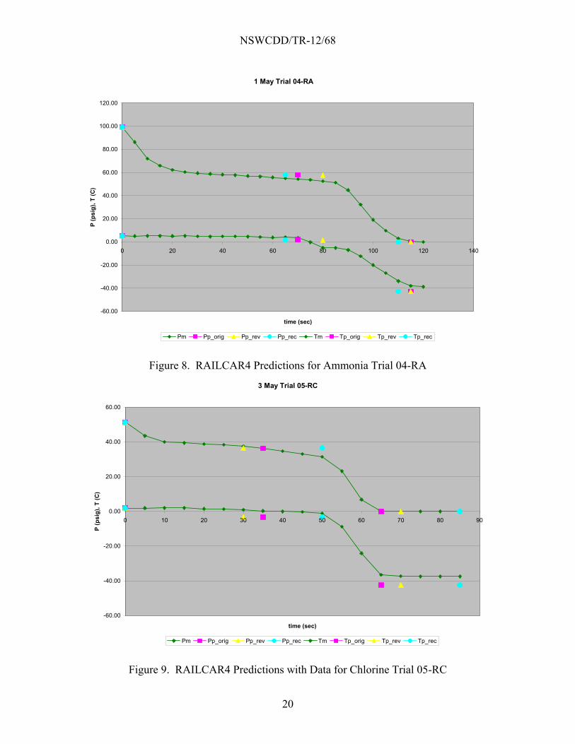
In conducting the final calibration, enough modifications were made to the program to result in a new RAILCAR4. The pool evaporation methodology was changed to use ground temperature for evaporating liquid pools and the chemical boiling temperature for boiling liquid pools; the chemical properties at the appropriate temperature are now obtained within that subroutine. Ground temperature was added as an input parameter. A correction was made to the liquid jet pressure drop to correctly account for the orifice vaporization. The sheltering factor of 5 was replaced by a user input to allow the cloud duration to be matched. Figures 8 and 9 show the fit and recommended temperature and pressure results with the RAILCAR3 results in Figures 6 and 7. The final prediction errors are displayed in Table 4.

NSWCDD/TR-12/68

20

1 May Trial 04-RA

-60.00

-40.00

-20.00

0.00

20.00

40.00

60.00

80.00

100.00

120.00

0 20 40 60 80 100 120 140

time (sec)

P (

ps

ig),

T (

C)

Pm Pp_orig Pp_rev Pp_rec Tm Tp_orig Tp_rev Tp_rec

Figure 8. RAILCAR4 Predictions for Ammonia Trial 04-RA

3 May Trial 05-RC

-60.00

-40.00

-20.00

0.00

20.00

40.00

60.00

0 10 20 30 40 50 60 70 80 90

time (sec)

P (

ps

ig),

T (

C)

Pm Pp_orig Pp_rev Pp_rec Tm Tp_orig Tp_rev Tp_rec

Figure 9. RAILCAR4 Predictions with Data for Chlorine Trial 05-RC

NSWCDD/TR-12/68

21

Table 4. RAILCAR4 Prediction Errors

absolute % error 7-Apr 8-Apr 27-Apr 1-May 3-Maychemical ammonia chlorine ammonia ammonia chlorinefinal temperature drop (°K) 7.8 7.4 6.0 8.6 12.4depress. temp. drop (°K) 92.9 1200.0 18.2 70.0 333.3depress. press. drop (atm) 17.6 13.8 6.7 8.7 4.1liquid empty time (s) 11.8 2.3 26.0 21.0 56.3tank empty time (s) 18.7 3.8 21.2 6.9 25.0cloud temperature drop (°K) 61.5 53.8 29.6 3.7 7.8cloud diameter (m) 49 22 26 17 17cloud duration (min) 15 73 8 60 3pool diameter (m) 30 50 10 18 12.5pool duration (min) 180 150 40 1 8off-gassing duration (min) NA NA 15 5 75

absolute % error 4-May 5-May 7-May 20-May 21-May averagechemical chlorine chlorine chlorine ammonia ammonia final temperature drop (°K) 13.1 10.8 13.2 10.9 16.5 10.7depress. temp. drop (°K) 36.6 107.7 51.5 12.8 2.4 192.5depress. press. drop (atm) 32.2 24.6 29.2 27.0 63.2 22.7liquid empty time (s) 4.3 6.0 5.4 0.0 16.7 15.0tank empty time (s) 30.6 17.6 20.5 6.1 13.8 16.4cloud temperature drop (°K) 16.9 37.7 11.7 NA NA 27.8cloud diameter (m) NA 0 5 68 NA 26cloud duration (min) NA 27 18 96 NA 38pool diameter (m) 17 17 17 10 10 19pool duration (min) 14 29 24 50 20 52off-gassing duration (min) 36 10 10 22 50 28

NSWCDD/TR-12/68

22

3.0 RAILCAR4 OPERATOR’S INSTRUCTIONS

This section guides the operator in using the RAILCAR4 program. The thermodynamic properties needed for each TIC are described in case the user needs to update physical properties or add data for a TIC not currently addressed by the program. The input parameters are discussed along with the supporting algorithms, where applicable. Guidance is then provided as to how best to interpret the output generated as inputs to transport and diffusion models for downwind toxic hazard area and concentration challenge level estimation. 3.1 TIC Thermodynamic Property File

Thermodynamic properties for each of the 44 chemicals addressed by RAILCAR4 have been extracted from reputable literature sources or estimated from accepted empirical relations.27-34 The thermodynamic properties for each chemical are contained in a single file named RAILCAR.PAR. This approach allows the user to substitute more reliable or acceptable values when they are located or measured. The approach also allows the user to add additional chemicals to the file if the appropriate thermodynamic properties are available. The format for each chemical is identical, with entries being separated by one or more spaces. RAILCAR4 is written in FORTRAN, with the numerical file entries read in free format. The records for each TIC in RAILCAR.PAR consist of 6 lines: Line Parameter(s) 1 character string for the TIC name (25-character limit) 2 freezing temperature (°C) critical temperature (°C) 3 molecular weight (g/mole) liquid viscosity at 20 °C (cp) liquid heat capacity (specific heat) at boiling temperature (kJ/kg-K) vapor heat capacity (specific heat) at boiling temperature (kJ/kg-K) liquid surface tension at boiling temperature (dynes/cm) vapor diffusivity at 20 °C (cm2/s)

4 liquid density at boiling temperature (kg/m3) liquid density rate of change with temperature (kg/m3-K)

5 Antoine constants A, B, and C for temperature in °C and pressure in atmospheres 6 heat of vaporization at boiling temperature (kJ/kg) heat of vaporization rate of change with temperature (kJ/kg-K) The chemicals in the file are in alphabetical order. The records created for nitric acid are listed in Figure 10. Liquid viscosity is only used for the jet flow rate at the tank liquid temperature, so the value should not be significantly different than that at 20 °C. Vapor and liquid heat capacity

NSWCDD/TR-12/68

23

values are adjusted for temperature within the program; the original mist pool methodology assumed the values are constant with temperature. Liquid surface tension is only used for aerosol formation during adiabatic expansion, which occurs at the TIC boiling temperature. Boiling temperature is computed from the Antoine constants for a pressure of 1 atm. Vapor diffusivity is used for pool evaporation and is also adjusted for temperature within the program; pool evaporation is not addressed by the mist pool methodology.

nitric acid -41.60 500.00 63.01 0.76 1.39 0.85 40.9 0.105 1503 -2.700 5.6270 2003.00 273.150 659.00 -0.952

Figure 10. Nitric Acid Thermodynamic Properties

Vapor pressure, liquid density, vapor density, and heat of vaporization are all relevant to multiple processes inside and outside of the tank, and a wide range of temperatures is relevant. Vapor density is computed from vapor pressure, temperature, and molecular weight using the ideal gas equation. These physical properties vary considerably with temperature. In general, the lowest temperature of interest is the greater of the freezing temperature and -100 °C for high-volatility chemicals and the higher of the freezing temperature and -20 °C for lower volatility chemicals. The highest temperature of interest is 50 °C, except in the case of chemicals that react and heat up when exposed to humid air or surface materials such as sulfuric acid. The temperature range for sulfuric acid file may extend to 200 °C. The temperature range of -20 °C to 50 °C is considered to cover the range of possible ambient temperatures, which usually also apply to the temperature of the liquid in the tank. RAILCAR.PAR is located in the same directory as the RAILCAR4 executable. 3.2 Input Parameters and Algorithms

RAILCAR4 has a total of 33 parameters entered or read as input for each run. The parameters can be entered by the user or read from an existing input data file. Not all of the parameters are relevant to every run. Since it is difficult to determine prior to a simulation which processes are relevant and which are not, all values must be entered.

1. TIC name: the name of the TIC to be released in the simulation. The character string must match one of the names in file RAILCAR.PAR.

2. Mass input type (1= chlorine tank size, 2= mass): the TIC masses in the tank and

remaining after the tank is empty can be entered by either mass in kilograms or in terms of the chlorine tank volume. For example, chlorine DOT 105A500W railcars are filled by weight to 90 tons chlorine liquid. If the user wishes to use the same railcar type with a different TIC, the user can enter 90 tons, and the program will calculate the correct fill

NSWCDD/TR-12/68

24

mass using relative liquid densities. The units of measurement are U.S. tons equal to 2000 lb rather than metric tons equal to 1000 kg. The liquid density of ammonia is 43.3% that of chlorine liquid, so the resulting ammonia fill mass will be (90 tons)(2000 lb/ton)(1kg/2.206 lb)(0.433)= 35,331 kg.

3. Initial tank mass: the mass in kilograms of TIC in the tank at the time of hole formation.

There is no range limit for mass in kilograms. If the mass input type (Parameter 2) is 1 (chlorine tank size) the number of tons of chlorine for that tank type is entered. The number of tons must be within the range of 1 ton to 200 tons.

4. Recovered liquid mass: the mass in kilograms of TIC liquid remaining in the tank after

depressurization is complete. If the mass input type (Parameter 2) is 1 (chlorine tank size), the number of tons of chlorine that would remain for the tank type and hole position is entered. The recovered liquid mass must be less than or equal to 50% of the initial liquid mass (Parameter 3), signifying that the hole is at or below the tank midpoint. RAILCAR4 assumes that the hole is generated in the liquid space of the tank, except for TICs that only exist as vapor at the tank temperature (Parameter 6) (i.e., tank temperature is above the critical temperature). For holes generated in the liquid space, whether pressurized liquid or liquids below their boiling temperatures, the liquid will empty to the level of the bottom of the hole. Pressurized liquids will auto-refrigerate to their boiling temperatures within the tank during depressurization. The resulting 1 atm vapor pressure is the same as the ambient pressure, so there will be no significant vapor flux out of the tank after that point. Liquids transported or stored below their boiling temperatures will already have a vapor pressure less than ambient pressure, so there will again be no significant vapor flux after the vapor-liquid interface reaches the bottom of the hole. There will be no tank depressurization for these liquids.

5. Air temperature: the temperature in °C of the ambient air at the time of hole formation.

Air temperature must be within the range of -15 °C to 50 °C, which is considered appropriate for relevant geographic locations. Air temperature is used for determining cloud equilibrium after air entrainment. RAILCAR4 does not allow for changes in meteorological conditions. If a mist pool or stationary cloud forms, vapor detrains into the passing air rather than air being entrained into the mist pool, so a change in air temperature will not affect the behavior of the mist pool/stationary cloud. Since meteorological conditions can be reasonably assumed to be constant for up to one hour, this RAILCAR4 restriction is only a limitation if the release duration or pool evaporation duration exceeds one hour.

6. Ground temperature: the temperature in °C of the ground at the time of hole formation.

Ground temperature must be within the range of -15 °C to 50 °C, which is considered appropriate for relevant geographic locations. Ground temperature is used for computing the liquid pool evaporation rate.

7. Tank temperature: the temperature in °C of the liquid and vapor in the tank at the time of

hole formation. There is no range limit for tank temperature, which allows for contents to be heated or refrigerated. For liquid pools that heat up due to reaction with surface

NSWCDD/TR-12/68

25

materials or humid air, the entered tank temperature should represent the temperature of the pool after heating. Tank temperature is expected to be within the range of validity for the thermodynamic property equations.

8. Relative humidity: the relative humidity in percent of the ambient air. Relative humidity

must be within the range of 0% to 100%. Relative humidity is used to determine air density and contributes to cloud equilibrium by cooling, condensing, and freezing. RAILCAR4 does not allow for changes in meteorological conditions. Since meteorological conditions can be reasonably assumed to be constant for up to one hour, this RAILCAR4 restriction is only a limitation if the release duration exceeds one hour.

9. Tank pressure: the initial pressure in atmospheres inside the tank if the tank temperature

(Parameter 7) exceeds the TIC critical temperature; there is no liquid phase in the tank.

10. Liquid head pressure mode (1= calculated, 2= user input): the tank volume and diameter for the entered initial tank mass (Parameter 3) and ullage volume fraction (Parameter 13) using the aspect ratio of the DOT 105A500W railcar. The angle to the vapor-liquid interface is then determined, which is then converted to liquid head pressure in atmospheres. This parameter allows the user to enter the liquid head pressure in place of these calculations.

11. Liquid head pressure: the pressure in atmospheres at the bottom of the tank due to the

height of liquid within the tank when the liquid head pressure mode (Parameter 10) is 2 (user-input). Liquid head pressure, Phead, follows the equation:

Pihead = ρL g HL/(101325 Pa/atm) [4]

where L is the liquid density in kg/m3, and HL is the liquid height in meters. There is no range limit for liquid head pressure. This parameter is not requested if the liquid head pressure mode (Parameter 10) is 1 (calculated).

12. Inert gas head pressure: the pressure in atmospheres of nitrogen, air, or any inert gas

added or trapped in the ullage space. There is no range limit for the inert gas head pressure. RAILCAR4 used the thermodynamic properties of dry air for the gas, regardless of composition. Since air is 79% nitrogen, there is little error in using air properties for this most commonly added gas. If any gas other than nitrogen or air is added, the thermodynamic properties may be significantly different. This parameter is not used if the tank temperature (Parameter 7) exceeds the TIC critical temperature, as there is no reason to have other than the all-vapor TIC inside the tank.

13. Ullage volume fraction: the fraction of tank volume not occupied by liquid. This space

will contain TIC vapor and any added or trapped inert vapor. The TIC vapor is assumed to be at equilibrium with the liquid, so the mass is determined by the vapor pressure at the tank temperature (Parameter 7). The practical range for this value is from 0 to less than 1. The typical ullage volume fraction recommended by RAILCAR4 is 0.2 if the user does not know the correct value. This parameter is not used if the tank temperature

NSWCDD/TR-12/68

26

(Parameter 7) exceeds the TIC critical temperature, as there is no reason to have other than the all-vapor TIC inside the tank.

14. Aerosol fraction rained out due to impaction: the fraction of liquid mass in aerosol form

following adiabatic expansion of the jet, which impacts the ground surface and forms a liquid pool. The range for this value is from 0 to 1. This parameter is reset to 1 if the tank temperature (Parameter 7) is below the TIC boiling temperature, as the jet will be all liquid with all of the mass depositing onto the ground surface. Similarly, RAILCAR4 assumes that a tank temperature less than 20 °C above the boiling temperature (i.e., liquid superheat) generates large droplets that also deposit onto the ground surface and resets the rainout fraction to 1. The rainout fraction recommended by RAILCAR4 is: 0.1 for ammonia, 0.5 for chlorine, and 0.3 for other chemicals, if the jet is aimed downward and 0 otherwise. The jet will be aimed downward if the hole is below the midpoint of the tank.

15. Tank thickness input type (1= default, 2= user input): the default tank thickness is based

on the combined thickness of 4.875 inches for the tank, insulation, and jacket for a DOT 105A500W railcar and 0.75 inches for a 1-ton chlorine tank. The larger thickness is assumed for any tank containing more than 5000 kg of liquid chemical. This parameter allows the user to define the tank thickness in place of these assumed values; 2 (user input) should also be selected for a pipe attached to the tank.

16. Tank thickness: the thickness in meters of the tank from the liquid inside to the air

interface if the tank thickness input type (Parameter 15) is 2 (user-input). If the incident involves rupture of a pipe attached to the tank or failure of a nozzle at the end of a pipe, this parameter represents the length of pipe between the liquid inside and the location of the rupture or nozzle. There is no range limit for the tank thickness or pipe length. RAILCAR4 combines the Bernoulli equation with frictional losses through the thickness of the tank or length of pipe. Based on observations during the Jack Rabbit pilot tests and field trials, there will be some vaporization before the hole opening if there is a pipe attached to the tank.

17. Hole/pipe parameter type (1= diameter, 2= area): the sizes of the hole and orifice can be

defined in terms of diameter in inches or area in square meters. 18. Equivalent hole/pipe diameter: the diameter in inches of the inner surface of the hole or

pipe if the hole/pipe parameter type (Parameter 17) is 1 (diameter). The inner diameter is assumed to be uniform through the thickness of the hole or length of the pipe up to the orifice if there is one. There is no range limit for hole and orifice diameter, but the jet flow methodology cannot be expected to be accurate for holes larger than about 12 inches in diameter.

19. Hole area: the inner area of the hole or pipe in square meters if the hole/pipe parameter

type (Parameter 17) is 2 (area). The inner diameter is assumed to be uniform through the thickness of the hole or length of the pipe up to the orifice if there is one. There is no

NSWCDD/TR-12/68

27

range limit for hole and orifice area, but the jet flow methodology cannot be expected to be accurate for holes larger than about 12 inches in diameter.

20. Orifice type (1= unrestricted, 2= restricted): an orifice can be placed at the air interface

of the hope or pipe to restrict flow, as designed for the Jack Rabbit pilot tests and field trials. RAILCAR4 assumes the transition between the hole or pipe and the orifice is smooth and does not add additional frictional losses other than due to the reduced area.

21. Orifice diameter: the diameter in inches of the inner surface of the orifice positioned at

the air interface of the hole or pipe if the hole/pipe parameter type (Parameter 17) is 1 (diameter). Although there is no check within RAILCAR4, the orifice diameter must be smaller than the hole diameter (Parameter 18). If the orifice type (Parameter 20) is 1 (unrestricted) the orifice diameter is set equal to the hole diameter.

22. Orifice area: the inner area in square meters of the orifice positioned at the air interface

of the hole or pipe if the hole/pipe parameter type (Parameter 17) is 2 (area). Although there is no check within RAILCAR4, the orifice area must be smaller than the hole area (Parameter 19). If the orifice type (Parameter 20) is 1 (unrestricted) the orifice area is set equal to the hole area.

23. Does foaming occur? (1= no, 2= yes): the extended depressurization time for Jack Rabbit pilot tests and field trials showed that the near-instantaneous pressure drop at the hole leads to foaming of the pressurized liquid within the tank ullage volume. Selection of 2 (yes) is recommended for releases of pressurized liquid. Foaming is not relevant to chemicals stored as all-vapor or chemicals stored at temperatures below the boiling temperature.

24. Percent liquid fill becoming foam: the percent of initial liquid that becomes foam mixed

with the initial vapor in the ullage volume. The range of this parameter is from 0 to 100. Based on the Jack Rabbit data, a value of 6.5% is recommended for pressurized liquids.

25. Minimum vaporization percent: the percent of liquid in the pipe that vaporizes prior to

the air interface. The range of this parameter is from 0 to 100. The slower liquid flow rate and shape of the jet during the Jack Rabbit pilot tests and field trials suggests that vaporization occurs if a pipe is attached to the tank. The recommended value for pressurized liquids is 3.5% if flow is through a pipe and 0% otherwise.

26. Pool mass fraction absorbing into ground: the fraction of mass in the boiling or

evaporating liquid pool that absorbs into the porous ground surface and off-gasses at a rate slower than pool evaporation after the liquid mass on the surface is gone. The range of this parameter is from 0 to 1. The ground surface in the pit progressively degraded with each pilot test and field trial due to the interaction of ammonia, chlorine, and ice with the soil around the tank. The field trials had visible vapor off-gassing well after the liquid sitting on the surface had evaporated. Although repeated incidents at the same location are not expected, a value of 0.25 is recommended if the surface is porous and 0 otherwise.

NSWCDD/TR-12/68

28

27. Liquid pool depth: the depth or thickness in centimeters of the boiling or evaporating liquid pool formed from rainout from the jet. There is no range limit for this parameter, but observations of liquid pools on fairly smooth surfaces suggest the pool depth will not exceed 1 cm. Pool depth is expected to be thicker on rough surfaces. Liquid pool formation is expected for chemicals stored at temperatures below the boiling temperature, chemicals stored at temperatures less than 20 °C above the boiling temperature, and chemicals stored at higher superheat where the jet impacts the ground surface. RAILCAR4 assumes that all liquid in the jet rains out for the first two cases and uses the aerosol fraction rained out due to impaction (Parameter 14) for the last case. A liquid pool will not form for chemicals stored as all-vapor. The recommended value is: 0.3 cm for ammonia, 1.2 cm for chlorine, and 0.8 cm for other chemicals.

28. Entrainment ratio: the volume of air mixed into the jet over the volume of the jet. This

parameter must be greater than or equal to zero. This parameter is used to determine if the mist pool or stationary vapor cloud formation criterion is met and to calculate the mist pool/stationary cloud behavior if it is. The recommended value, based on the Jack Rabbit data, is 180. A mist pool or stationary vapor cloud will not form for chemicals stored at temperatures below the boiling temperature. A stationary vapor cloud may form for chemicals stored as all-vapor due to formation of a very cold cloud upon expansion to ambient pressure. RAILCAR4 uses a volumetric air entrainment ratio of 20 for such a release due to lack of data; the RAILCAR4 stationary vapor cloud algorithms may not work properly for an all-vapor release.

29. Cloud height: the height or thickness in meters of the mist pool or stationary vapor cloud

after formation. This parameter must be greater than 0 m. Like the entrainment ratio (Parameter 28), this parameter is used to determine if the mist pool or stationary vapor cloud formation criterion is met and to calculate the mist pool/stationary cloud behavior if it is. The recommended value is 4 m. A mist pool or stationary vapor cloud will not form for chemicals stored at temperatures below the boiling temperature. A stationary vapor cloud may form for chemicals stored as all-vapor due to formation of a very cold cloud upon expansion to ambient pressure. RAILCAR4 uses a cloud height of 1 m for such a release due to lack of data; the RAILCAR4 stationary vapor cloud algorithms may not work properly for an all-vapor release.

30. Wind speed at 2 m height: the surface wind speed in meters per second at the release

location. There is no range limit for this parameter. This parameter is only used for the liquid pool evaporation calculations. For the Jack Rabbit pilot tests and field trials, the appropriate wind speed was taken by the anemometer in the pit. RAILCAR4 does not allow for changes in meteorological conditions. Since meteorological conditions can be reasonably assumed to be constant for up to one hour, this RAILCAR4 restriction is only a limitation if the pool evaporation duration exceeds one hour. If the 2-m wind speed is not known for user input, it can be estimated from other parameters, which include 10-m wind speed, friction velocity, surface type, and atmospheric stability. Wind condition input is described in Section 3.3.

NSWCDD/TR-12/68

29

31. Friction velocity: the friction velocity in meters per second for the level of turbulence in the surface winds due to surface heating or cooling and interaction with the roughness elements of the ground surface. This parameter must be greater than 0 m/s. It is used to determine if a mist pool or stationary vapor cloud will form and to determine the resulting behavior if one does. For the Jack Rabbit pilot tests and field trials, the appropriate wind speed used to determine the friction velocity was taken by the anemometers just outside of the pit. RAILCAR4 does not allow for changes in meteorological conditions. Since meteorological conditions can be reasonably assumed to be constant for up to one hour, this RAILCAR4 restriction is only a limitation if the release duration exceeds one hour. If the friction velocity is not known for user input, it can be estimated from other parameters, which include 2-m wind speed, 10-m wind speed, surface type, and atmospheric stability. Wind condition input is described in Section 3.3.

32. Entrainment factor (1= enhanced, 2= normal, 3= sheltered): this parameter provides a

rough characterization of the interaction of the jet with passing air. It is used to determine if the mist pool or stationary vapor cloud formation criterion is met and to calculate the mist pool/stationary cloud behavior if it is. An entrainment factor of 1 (enhanced) is appropriate if entrainment of the jet into the passing air is enhanced by the jet aiming upwards or with the wind or the terrain is flat and smooth; the mist pool algorithms then multiply the vapor flux by the sheltering factor (Parameter 33). An entrainment factor of 3 (sheltered) is appropriate if entrainment is inhibited by the presence of buildings, vegetation, and/or terrain undulations at the release location that shelter the jet from the ambient wind; the mist pool algorithms then divide the vapor flux by the sheltering factor (Parameter 33). An entrainment factor of 2 (normal) is appropriate if entrainment is neither enhanced nor sheltered, and a factor of 1 is used in the mist pool algorithms.

33. Sheltering factor: the value which the air entrainment ratio is multiplied by if the

Entrainment factor (Parameter 33) is 1 (enhanced) and divided by if the Entrainment factor is 3 (sheltered). This value is not used if the Entrainment factor is 2 (normal). The sheltering factor must be greater than one. The recommended value is: 1.5 for ammonia, 4.5 for chlorine, and 3.0 for other chemicals.

3.3 Wind Condition Input

The wind speed at 2-m height and friction velocity at the release location are required inputs. These parameters are recorded to the input file. If user input is selected instead of file input and the user does not know either of these values, the user is prompted for alternate parameters that are used to estimate them. There are four combinations of meteorology parameters that can be used, the first of which is the 2-m wind speed and friction velocity, both in meters per second.

The second option is relevant if the friction velocity is known, but the wind speed measurement height is 10 m instead of 2 m. In order to determine the 2-m wind speed, the

NSWCDD/TR-12/68

30

surface type is needed. The surface type is used to compute the surface roughness length in meters. The user is first prompted to enter the friction velocity and 10-m wind speed, both in meters per second. A second prompt is then displayed:

enter surface type 1 - water 2 - urban 3 - sand 4 - barren 5 - grass 6 - brush 7 - forest 8 - know roughness length

The surface types are listed in order of increasing surface roughness length, which ranges from 0.001 m to 0.4 m. Alternately, the user may enter the value in meters if known.

The third option is relevant if the 2-m wind speed is known, but the friction velocity is not. In order to determine the friction velocity, the surface type and the Pasquill stability category are needed. The surface type is used to compute the surface roughness length in meters, and the Pasquill stability category is used to compute the Monin-Obukhov length, which characterizes the depth in meters of the surface layer turbulence. The user is first prompted to enter the 2-m wind speed in meters per second. The surface type prompt above is then displayed. A third prompt then appears:

enter Pasquill stability category 1 - highly unstable 2 - unstable 3 - slightly unstable 4 - neutral 5 - slightly stable 6 - stable 7 - highly stable 8 - know Monin-Obukhov length

The last selection allows the user to enter the value for the Monin-Obukhov length in meters. Monin-Obukhov length is negative for unstable conditions, positive for stable conditions, and very large for neutral conditions.

The fourth option is relevant if the 10-m wind speed is known, and the friction velocity is not. In order to determine the 2-m wind speed and friction velocity, the surface type and the Pasquill stability category are needed. The surface type is used to compute the surface roughness length in meters, and the Pasquill stability category is used to compute the Monin-Obukhov length in meters. The user is first prompted to enter the 10-m wind speed in meters per second. The surface type prompt above is then displayed, followed by the Pasquill stability category prompt.

User entries for 10-m wind speed, surface type, surface roughness length, Pasquill stability category, and/or Monin-Obukhov length are not recorded to the output file. The 2-m wind speed is output with the pool evaporation summary, and the friction velocity is output with the mist pool/stationary cloud summary.

NSWCDD/TR-12/68

31

3.4 Executing the Program

RAILCAR4 currently has no graphical interface and operates in a character graphics mode; it has been compiled for operation on a Windows PC. The RAILCAR4 executable is started by using the Windows run command or by double-clicking on the executable icon. All of the RAILCAR4 input files (e.g., RAILCAR.PAR and RAILCAR.DAT) must exist in the same directory as the executable, and the output file RAILCAR.OUT is generated in that same directory. Upon execution, a character graphics window is opened, and displays the following prompt: enter mode of parameter input 1 = file 2 = user-entered If 1 (file) is entered the next prompt is enter name of input file (return = RAILCAR.DAT)

The default input file name and the one that is created if the user selects a mode of parameter input of 2 (user-entered) is RAILCAR.DAT. For that parameter input mode, the user is prompted with the list of available TICs shown in Figure 11. This prompt is then followed by prompts for the other 32 parameters described in Section 3.2. File RAILCAR.DAT is created after all parameters have been defined; if RAILCAR.DAT already exists, it is overwritten with the new parameter values. The file is not created if the input parameters were read from a file. An example RAILCAR.DAT for the Jack Rabbit ammonia pilot test is provided in Figure 12. The order of the parameters is the same as in Section 3.2 except for the 6th line. The parameters in that line are: hole/pipe parameter type, orifice type, equivalent hole/pipe diameter, orifice diameter, hole area, orifice area.

Figure 11. RAILCAR TIC List

NSWCDD/TR-12/68

32

ammonia 2 907.0000000 0.0000000 -0.1000000 0.7000000 -0.5000000 78.0000000 0.0000000 2 0.0300000 2.1299999 0.6000000 0.0600000 2 0.4100000 1 2 4.0000000 2.0000000 0.0000000 0.0000000 1 15.0000000 3.5000000 0.0000000 0.0780000 0.3000000 290.0000000 1.7000000 4 0.0160000 3 4.1000000

Figure 12. Example RAILCAR.DAT File

The user can create RAILCAR4 input files by renaming RAILCAR.DAT. These files are text files that can also be edited using programs such as NOTEPAD, so changes can be made to RAILCAR.DAT and saved under a different name to create as many input files as desired. Other than the first line containing the name of the toxic industrial chemical, the input files are free format separated by spaces.

Once the input parameters have been defined from a file or user input, the calculations begin. RAILCAR4 creates output file RAILCAR.OUT and also records status and output information to the character graphics window. The output displayed on the screen is almost identical to that recorded in the output file and is described in Section 3.5. Upon completion of the simulation, the following prompt is displayed: enter 1 to restart and -1 to exit After the user responds, the message end of run is displayed, and the program either returns to the first prompt above or closes the character graphics window and terminates. File RAILCAR.OUT remains open until the program is terminated, so each simulation is appended to the previous one in that file. 3.5 Interpreting the Output File

The RAILCAR4 calculations are divided into the physical processes being simulated. The processes have times and durations associated with them, but RAILCAR4 does not use time steps. This section describes the processes and the information displayed on the screen and recorded to RAILCAR.OUT. The output associated with the input parameters contained in Figure 12 for the Jack Rabbit ammonia pilot test is used as an example addressing almost all of the relevant physical processes.

The first output is a summary of some of the physical properties read from the thermodynamic property file for the TIC.

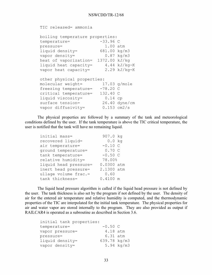
NSWCDD/TR-12/68

33

TIC released= ammonia

boiling temperature properties: temperature= -33.96 C pressure= 1.00 atm liquid density= 681.00 kg/m3 vapor density= 0.87 kg/m3 heat of vaporization= 1372.00 kJ/kg liquid heat capacity= 4.44 kJ/kg-K vapor heat capacity= 2.29 kJ/kg-K

other physical properties: molecular weight= 17.03 g/mole freezing temperature= -78.20 C critical temperature= 132.40 C liquid viscosity= 0.14 cp surface tension= 26.40 dyne/cm vapor diffusivity= 0.153 cm2/s

The physical properties are followed by a summary of the tank and meteorological

conditions defined by the user. If the tank temperature is above the TIC critical temperature, the user is notified that the tank will have no remaining liquid.

initial mass= 907.0 kg recovered liquid= 0.0 kg air temperature= -0.10 C ground temperature= 0.70 C tank temperature= -0.50 C relative humidity= 78.00% liquid head pressure= 0.0300 atm inert head pressure= 2.1300 atm ullage volume frac.= 0.60 tank thickness= 0.4100 m

The liquid head pressure algorithm is called if the liquid head pressure is not defined by

the user. The tank thickness is also set by the program if not defined by the user. The density of air for the entered air temperature and relative humidity is computed, and the thermodynamic properties of the TIC are interpolated for the initial tank temperature. The physical properties for air and water vapor are stored internally to the program. They are also provided as output if RAILCAR4 is operated as a subroutine as described in Section 3.6.

initial tank properties: temperature= -0.50 C vapor pressure= 4.18 atm pressure= 6.31 atm liquid density= 639.78 kg/m3 vapor density= 5.94 kg/m3

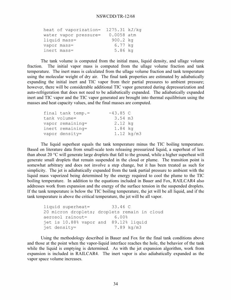
NSWCDD/TR-12/68

34

heat of vaporization= 1275.31 kJ/kg water vapor pressure= 0.0058 atm liquid mass= 900.2 kg vapor mass= 6.77 kg inert mass= 5.86 kg

The tank volume is computed from the initial mass, liquid density, and ullage volume

fraction. The initial vapor mass is computed from the ullage volume fraction and tank temperature. The inert mass is calculated from the ullage volume fraction and tank temperature using the molecular weight of dry air. The final tank properties are estimated by adiabatically expanding the initial inert and TIC vapor from their partial pressures to ambient pressure; however, there will be considerable additional TIC vapor generated during depressurization and auto-refrigeration that does not need to be adiabatically expanded. The adiabatically expanded inert and TIC vapor and the TIC vapor generated are brought into thermal equilibrium using the masses and heat capacity values, and the final masses are computed.

final tank temp.= -43.85 C tank volume= 3.54 m3 vapor remaining= 2.12 kg inert remaining= 1.84 kg vapor density= 1.12 kg/m3

The liquid superheat equals the tank temperature minus the TIC boiling temperature.

Based on literature data from small-scale tests releasing pressurized liquid, a superheat of less than about 20 °C will generate large droplets that fall to the ground, while a higher superheat will generate small droplets that remain suspended in the cloud or plume. The transition point is somewhat arbitrary and does not involve a step change, but it has been treated as such for simplicity. The jet is adiabatically expanded from the tank partial pressure to ambient with the liquid mass vaporized being determined by the energy required to cool the plume to the TIC boiling temperature. In addition to the equations included in Bauer and Fox, RAILCAR4 also addresses work from expansion and the energy of the surface tension in the suspended droplets. If the tank temperature is below the TIC boiling temperature, the jet will be all liquid, and if the tank temperature is above the critical temperature, the jet will be all vapor.

liquid superheat= 33.46 C 20 micron droplets; droplets remain in cloud aerosol rainout= 6.00% jet is 10.88% vapor and 89.12% liquid jet density= 7.89 kg/m3

Using the methodology described in Bauer and Fox for the final tank conditions above

and those at the point when the vapor-liquid interface reaches the hole, the behavior of the tank while the liquid is emptying is determined. As with the jet expansion algorithm, work from expansion is included in RAILCAR4. The inert vapor is also adiabatically expanded as the vapor space volume increases.

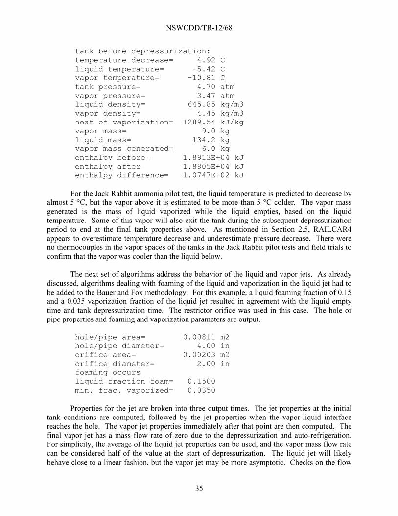
NSWCDD/TR-12/68

35

tank before depressurization: temperature decrease= 4.92 C liquid temperature= -5.42 C vapor temperature= -10.81 C tank pressure= 4.70 atm vapor pressure= 3.47 atm liquid density= 645.85 kg/m3 vapor density= 4.45 kg/m3 heat of vaporization= 1289.54 kJ/kg vapor mass= 9.0 kg liquid mass= 134.2 kg vapor mass generated= 6.0 kg enthalpy before= 1.8913E+04 kJ enthalpy after= 1.8805E+04 kJ enthalpy difference= 1.0747E+02 kJ

For the Jack Rabbit ammonia pilot test, the liquid temperature is predicted to decrease by

almost 5 °C, but the vapor above it is estimated to be more than 5 °C colder. The vapor mass generated is the mass of liquid vaporized while the liquid empties, based on the liquid temperature. Some of this vapor will also exit the tank during the subsequent depressurization period to end at the final tank properties above. As mentioned in Section 2.5, RAILCAR4 appears to overestimate temperature decrease and underestimate pressure decrease. There were no thermocouples in the vapor spaces of the tanks in the Jack Rabbit pilot tests and field trials to confirm that the vapor was cooler than the liquid below.

The next set of algorithms address the behavior of the liquid and vapor jets. As already discussed, algorithms dealing with foaming of the liquid and vaporization in the liquid jet had to be added to the Bauer and Fox methodology. For this example, a liquid foaming fraction of 0.15 and a 0.035 vaporization fraction of the liquid jet resulted in agreement with the liquid empty time and tank depressurization time. The restrictor orifice was used in this case. The hole or pipe properties and foaming and vaporization parameters are output.

hole/pipe area= 0.00811 m2 hole/pipe diameter= 4.00 in orifice area= 0.00203 m2 orifice diameter= 2.00 in foaming occurs liquid fraction foam= 0.1500 min. frac. vaporized= 0.0350

Properties for the jet are broken into three output times. The jet properties at the initial

tank conditions are computed, followed by the jet properties when the vapor-liquid interface reaches the hole. The vapor jet properties immediately after that point are then computed. The final vapor jet has a mass flow rate of zero due to the depressurization and auto-refrigeration. For simplicity, the average of the liquid jet properties can be used, and the vapor mass flow rate can be considered half of the value at the start of depressurization. The liquid jet will likely behave close to a linear fashion, but the vapor jet may be more asymptotic. Checks on the flow

NSWCDD/TR-12/68

36

equations are included to prevent the jet velocity from exceeding the speed of sound (i.e., choked flow) for liquid, vapor, or two-phase flow. For this example, the liquid empty time is estimated to be 35 seconds, followed by a 41-second depressurization time.

initial jet properties: fraction vaporized= 0.0350 liq. speed of sound= 1804.44 m/s liquid jet is not choked jet velocity= 166.49 m/s jet density= 63.14 kg/m3 pressure drop= 0.0918 atm Reynolds number= 1.9074E+06 mass flow rate= 21.31 kg/s final jet properties: fraction vaporized= 0.0350 liq. speed of sound= 1796.01 m/s liquid jet is not choked jet velocity= 136.84 m/s jet density= 82.72 kg/m3 pressure drop= 0.0687 atm Reynolds number= 2.0536E+06 mass flow rate= 22.94 kg/s average jet properties: average jet velocity= 151.67 m/s avg. mass flow rate= 22.12 kg/s liquid mass expulsed= 763.8 kg liquid empty time= 34.5 s initial vapor jet properties: foam speed of sound= 1701.42 m/s vapor jet is not choked jet velocity= 371.13 m/s jet density= 9.29 kg/m3 pressure drop= 0.0668 atm Reynolds number= 6.2579E+06 mass flow rate= 6.99 kg/s average velocity= 185.56 m/s average flow rate= 3.50 kg/s vapor mass expulsed= 145.1 kg inert mass expulsed= 4.02 kg depress. time= 41.5 s combined jet properties: avg. mass flow rate= 11.96 kg/s tank empty time= 76.0 s

If the jet is all-vapor, no liquid jet output is recorded, and an all-liquid jet will have no

vapor jet output. If a liquid pool is determined to form or is specified by the user to reflect rainout due to ground impaction of the jet, the characteristics of the pool are simulated. The mist

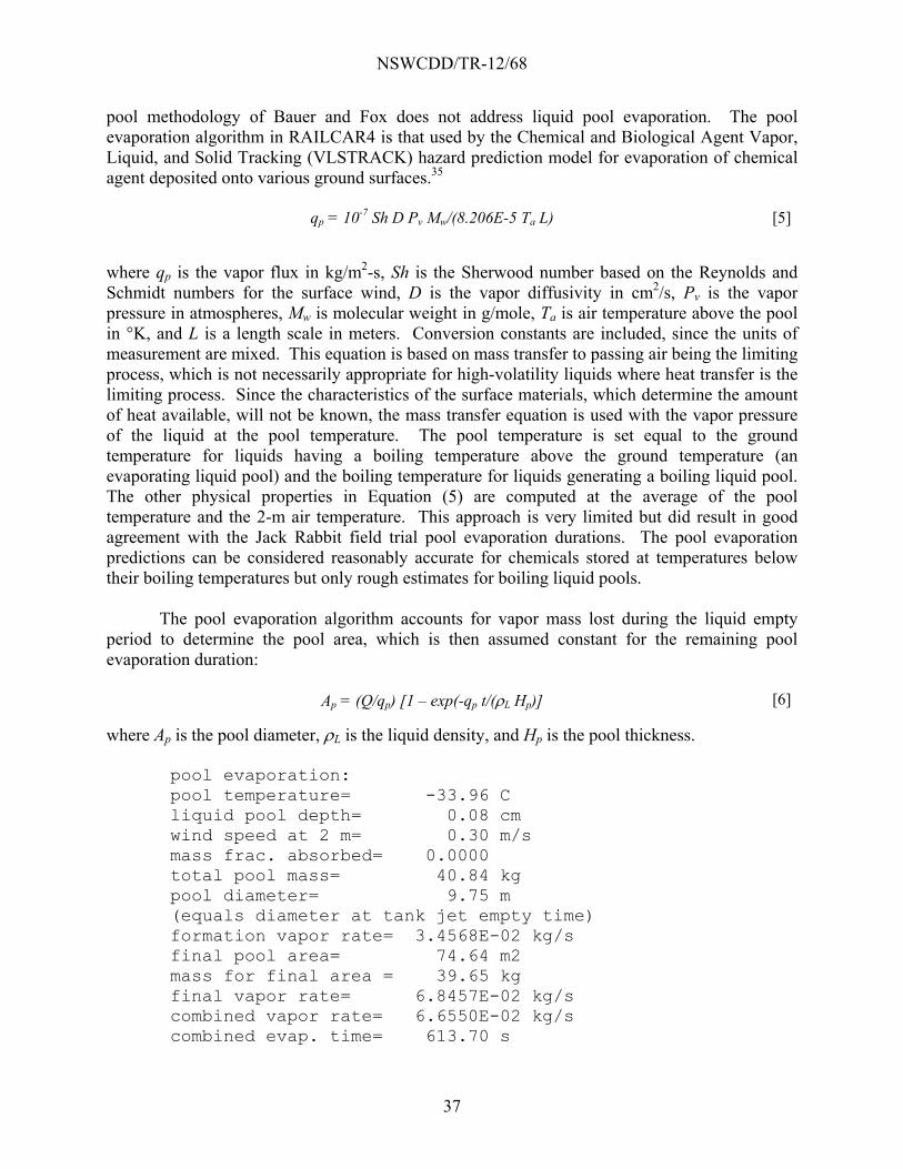
NSWCDD/TR-12/68

37

pool methodology of Bauer and Fox does not address liquid pool evaporation. The pool evaporation algorithm in RAILCAR4 is that used by the Chemical and Biological Agent Vapor, Liquid, and Solid Tracking (VLSTRACK) hazard prediction model for evaporation of chemical agent deposited onto various ground surfaces.35

qp = 10-7 Sh D Pv Mw/(8.206E-5 Ta L) [5]

where qp is the vapor flux in kg/m2-s, Sh is the Sherwood number based on the Reynolds and Schmidt numbers for the surface wind, D is the vapor diffusivity in cm2/s, Pv is the vapor pressure in atmospheres, Mw is molecular weight in g/mole, Ta is air temperature above the pool in °K, and L is a length scale in meters. Conversion constants are included, since the units of measurement are mixed. This equation is based on mass transfer to passing air being the limiting process, which is not necessarily appropriate for high-volatility liquids where heat transfer is the limiting process. Since the characteristics of the surface materials, which determine the amount of heat available, will not be known, the mass transfer equation is used with the vapor pressure of the liquid at the pool temperature. The pool temperature is set equal to the ground temperature for liquids having a boiling temperature above the ground temperature (an evaporating liquid pool) and the boiling temperature for liquids generating a boiling liquid pool. The other physical properties in Equation (5) are computed at the average of the pool temperature and the 2-m air temperature. This approach is very limited but did result in good agreement with the Jack Rabbit field trial pool evaporation durations. The pool evaporation predictions can be considered reasonably accurate for chemicals stored at temperatures below their boiling temperatures but only rough estimates for boiling liquid pools.

The pool evaporation algorithm accounts for vapor mass lost during the liquid empty period to determine the pool area, which is then assumed constant for the remaining pool evaporation duration:

Ap = (Q/qp) [1 – exp(-qp t/(L Hp)] [6]

where Ap is the pool diameter, L is the liquid density, and Hp is the pool thickness.

pool evaporation: pool temperature= -33.96 C liquid pool depth= 0.08 cm wind speed at 2 m= 0.30 m/s mass frac. absorbed= 0.0000 total pool mass= 40.84 kg pool diameter= 9.75 m (equals diameter at tank jet empty time) formation vapor rate= 3.4568E-02 kg/s final pool area= 74.64 m2 mass for final area = 39.65 kg final vapor rate= 6.8457E-02 kg/s combined vapor rate= 6.6550E-02 kg/s combined evap. time= 613.70 s

NSWCDD/TR-12/68

38

If liquid off-gassing occurs due to absorption of liquid into the ground surface, the time at

which the mass fraction in the surface liquid is gone is computed. The remaining liquid within the ground surface is then assumed to off-gas at a rate equal to 25% of the pool evaporation rate. Key output for pool evaporation includes the pool diameter at the tank empty time, the evaporation rates during formation, evaporation, and off-gassing, and the durations for evaporation and off-gassing. Pool durations are limited to 24 hours for output formatting reasons.

If the chemical is stored below its boiling temperature, no mist pool or stationary cloud will form. The message no mist pool forms is displayed, and the simulation skips the cloud property computations. Otherwise, the simulation moves to the mist pool algorithms. The mass considered for the mist pool formation criterion includes the mass from the liquid jet, the chemical and inert mass from tank depressurization, the air entrained into the jet, and the vapor from pool evaporation during the tank empty time. This last mass is computed from the pool evaporation rates and the tank empty time. Before plugging values into the mist pool criterion in Equations (1) to (3), a determination needs to be made as to whether the cloud will contain aerosol (a mist pool) or will be all vapor (a stationary vapor cloud) from the entered volumetric air entrainment ratio. RAILCAR4 contains an algorithm that determines the air entrainment ratio at which point all aerosol evaporates. This point is also the coldest potential cloud temperature, as the aerosol evaporation removes energy from the cloud without any additional energy being added by excess air. If the source is all-vapor or no aerosol is present due to rainout or jet expansion, the message no liquid aerosol present in cloud entrainment volume to evaporate aerosol equals 0 is displayed. Determining the maximum entrainment ratio requires an iterative process on the cloud temperature. Cloud cooling from aerosol can lead to temperatures well below the chemical boiling temperature, but the cloud temperature is not allowed to drop below the chemical freezing temperature. A message is displayed if the temperature iterations reach the freezing temperature: temperature reset to freezing temperature The properties at the maximum entrainment ratio are then determined.

entrainment ratio= 290.00 maximum entrainment ratio= 79.33 minimum cloud temperature= -71.41 C equilibrium vapor press.= 0.11 atm

NSWCDD/TR-12/68

39

If the entered entrainment ratio is equal to or below the maximum entrainment ratio, a mist pool will form if the criterion is met. If the entered entrainment ratio is above the maximum entrainment ratio, a stationary vapor cloud will form if the criterion is met.

The cloud temperature, density, concentration, and diameter are needed for the mist pool formation criterion. The next set of algorithms then applies the mist pool methodology for homogeneous equilibrium to determine the cloud properties for the masses described above. Other than the cloud diameter and height, the cloud temperature, density, and concentration characterize the plume following adiabatic expansion, air entrainment, and homogeneous equilibrium if the mist pool criterion is not met. The methodology defined by Bauer and Fox has been extended to allow for complete aerosol evaporation and subsequent cloud warming resulting from a volumetric air entrainment ratio exceeding the maximum entrainment ratio computed in the previous algorithm. A similar iterative solution on temperature to the maximum entrainment ratio algorithm is used for the cloud property algorithm, so the same limit on freezing temperature is applied and uses the same display message. RAILCAR4 outputs a summary of the properties calculated for the mist pool, stationary cloud, or plume that includes the cloud temperature, density, and concentration. The plume diameter is needed to characterize the source if a mist pool or stationary cloud is not formed. The diameter represents the plume after the jet has equilibrated with the entrained air.

final cloud properties: temperature= -20.14 C heat of vaporization= 1332.06 kJ/kg water fraction not freezing= 0.48864 aerosol evaporation fraction= 1.00000 partial pressure= 0.0331 atm saturation pressure= 1.8939 atm water vapor pressure= 2.2047E-03 atm ambient water vapor fraction= 0.00281 ambient air density= 1.2903 kg/m3 dry air density= 1.2867 kg/m3 water vapor density= 0.0036 kg/m3 cloud liquid density= 663.97 kg/m3 cloud density= 1.3766 kg/m3 cloud concentration= 0.0272 kg/m3 cloud is 1.07 times that of air plume diameter= 2.56 m

The final set of algorithms includes the mist pool criterion and the mist pool methodology

for releases meeting the criterion. The Richardson number of the cloud after assumed formation is computed using Equation (3) and displayed and recorded. A mist pool cannot form if the Richardson number is for neutral conditions (Ri* = 0) or positively buoyant (Ri* > 0), so a message is displayed if either condition exists: mist pool will not form

NSWCDD/TR-12/68

40

at which point the cloud property computations are complete; otherwise, the ratio of vapor mass entrainment rate over jet mass flow rate (i.e., mist pool ratio) is computed, displayed, and recorded. The same message is displayed if the ratio is greater than or equal to one, and the cloud property computations are again complete. In order to avoid unrealistically low vapor mass entrainment rates, the Richardson number for the mist pool criterion and the following mist pool behavior equations is limited to a value of 100. If the mist pool ratio is less than one, RAILCAR4 computes and outputs the total mass, chemical mass, liquid mass, and vapor mass in what will now be either a mist pool or a stationary cloud. A chemical liquid mass of 0 kg, as in the example below, signifies that no aerosol is present, and the cloud is a stationary vapor cloud.

cloud height= 1.70 m friction velocity= 0.0160 m/s cloud Richardson number= 4358.8 entrainment factor= 0.24 mist pool ratio= 0.0024 cloud mass= 43977.4 kg chemical mass= 868.1 kg chemical liquid mass= 0.0 kg chemical vapor mass= 868.1 kg

RAILCAR4 then proceeds to compute the properties of the mist pool or stationary vapor

cloud at each of the stages defined in Section 2. The first stage involves formation of the mist pool during the tank empty time, which includes the time for tank depressurization. Although vapor mass is entrained by passing air during this stage, Bauer and Fox do not adjust the cloud diameter for the mass lost during cloud formation. As with the liquid pool formation, RAILCAR4 accounts for vapor mass lost during the tank empty period to determine the cloud area, which is then assumed constant for the remaining mist pool/stationary vapor cloud duration:

Ac = (Qf /qv1) [1 – exp(-qv1 (t + td)/(c Hc)] [7]

where Ac is the cloud diameter, Qf is the average jet mass flow rate for the liquid empty time plus depressurization time, qv1 is the vapor flux in kg/m2-s, td is the tank depressurization duration, c is the cloud density, and Hc is the cloud thickness. If there is no aerosol present in the cloud, the message no aerosol present; stage 2 skipped is displayed. If it is determined that there is aerosol retained in the jet but the aerosol evaporates from air entrainment, the message all aerosol will evaporate while the tank empties stage 2 skipped

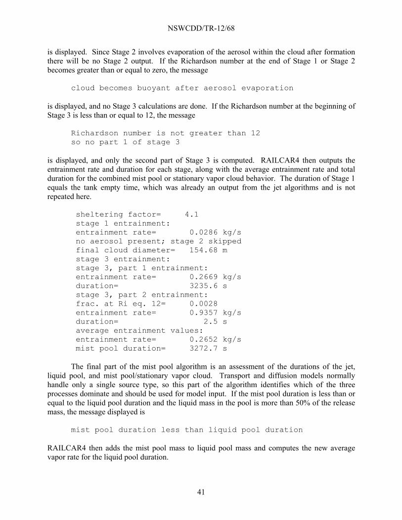
NSWCDD/TR-12/68

41

is displayed. Since Stage 2 involves evaporation of the aerosol within the cloud after formation there will be no Stage 2 output. If the Richardson number at the end of Stage 1 or Stage 2 becomes greater than or equal to zero, the message cloud becomes buoyant after aerosol evaporation is displayed, and no Stage 3 calculations are done. If the Richardson number at the beginning of Stage 3 is less than or equal to 12, the message Richardson number is not greater than 12 so no part 1 of stage 3 is displayed, and only the second part of Stage 3 is computed. RAILCAR4 then outputs the entrainment rate and duration for each stage, along with the average entrainment rate and total duration for the combined mist pool or stationary vapor cloud behavior. The duration of Stage 1 equals the tank empty time, which was already an output from the jet algorithms and is not repeated here.

sheltering factor= 4.1 stage 1 entrainment: entrainment rate= 0.0286 kg/s no aerosol present; stage 2 skipped final cloud diameter= 154.68 m stage 3 entrainment: stage 3, part 1 entrainment: entrainment rate= 0.2669 kg/s duration= 3235.6 s stage 3, part 2 entrainment: frac. at Ri eq. 12= 0.0028 entrainment rate= 0.9357 kg/s duration= 2.5 s average entrainment values: entrainment rate= 0.2652 kg/s mist pool duration= 3272.7 s

The final part of the mist pool algorithm is an assessment of the durations of the jet,

liquid pool, and mist pool/stationary vapor cloud. Transport and diffusion models normally handle only a single source type, so this part of the algorithm identifies which of the three processes dominate and should be used for model input. If the mist pool duration is less than or equal to the liquid pool duration and the liquid mass in the pool is more than 50% of the release mass, the message displayed is mist pool duration less than liquid pool duration RAILCAR4 then adds the mist pool mass to liquid pool mass and computes the new average vapor rate for the liquid pool duration.

NSWCDD/TR-12/68

42

If the mist pool duration is within 10% of the tank empty time, the initial source will be a plume having the diameter output with the final cloud properties. The message displayed is mist pool duration is similar to tank empty time

The liquid pool will still be the dominant source if the criteria above are met. A plume should only form from a pressurized liquid for a chemical stored at a temperature above its critical temperature. Other chemicals should form a liquid pool. Adiabatic expansion of the jet with a low air entrainment ratio such as 5 will lead to a plume diameter approximately 20 times the hole diameter. Adiabatic expansion of the jet with a high air entrainment ratio such as 100 will lead to a plume diameter approximately 100 times the hole diameter. All-vapor TICs do not expand from liquid evaporation, so the plume diameter will be due to adiabatic vapor expansion and air entrainment. The low air entrainment ratio and high air entrainment ratio plume diameters become approximately 2 and 10 times the hole diameter, respectively.

If the mist pool duration is between 1.1 and 5 times the tank empty time, the message displayed is mist pool area versus time must be considered The cloud will grow from zero to the diameter output for the tank empty time, with the vapor rate increasing linearly with cloud diameter to the value output for Stage 1. The vapor rate after cloud formation will follow the values output for Stages 2 and 3. If the mist pool duration is at least five times the tank empty time, which is the case for the ammonia example, the message displayed is mist pool can be assumed to form instantaneously If no mist pool forms, the source type(s) will be a plume and/or a liquid pool.

After all of the physical property computations are completed, a summary of key predicted source properties is presented:

Source Characterization Summary: final tank temp.= -43.85 C depress. temperature= -5.42 C depress. pressure= 4.70 atm liquid empty time= 34.5 s liquid jet flow rate= 22.1247 kg/s tank empty time= 76.0 s avg. jet flow rate= 11.9553 kg/s plume diameter= 2.56 m pool diameter= 9.75 m pool duration= 613.7 s max. pool mass rate= 0.0685 kg/s off-gassing duration= 613.7 s avg. pool mass rate= 0.0666 kg/s

NSWCDD/TR-12/68

43

cloud diameter= 154.68 m cloud temperature= -20.14 C cloud duration= 3272.7 s cloud vap. mass rate= 0.2652 kg/s

RAILCAR4 then determined the most appropriate source type of plume vapor source or

area vapor source, and the simplified vapor source properties of diameter, duration, and mass rate are presented. They are also provided as output if RAILCAR4 is operated as a subroutine as described in Section 3.6. The diameter, duration, and mass rate for the other source type are all set to zero. The “end of run” output appears for all simulations, as mentioned in Section 3.4.

Area vapor source properties: diameter= 154.68 m duration= 3272.7 s vapor mass rate= 0.2765 kg/s end of run

The output for the Jack Rabbit ammonia pilot test used as an example can now be

interpreted for input into a hazard assessment model for either sophisticated source characterization or simple source characterization. The test has a tank empty time of 76.0 s. The liquid jet lasts 34.5 s at a mass flow rate of 22.12 kg/s. Adding in the two-phase jet from depressurization decreases the mass flow rate to 11.96 kg/s. The diameter of the jet if no mist pool or stationary vapor cloud is formed is 2.56 m. The pool evaporation duration is 613.7 s. The pool diameter grows to 9.75 m over the 76.0 s tank empty time, at which point the pool vapor mass rate equals 0.0685 kg/s. No liquid absorbs into the ground, so there is no off-gassing duration. Accounting for the lower vapor flux of the liquid pool as it grows to its final diameter results in an average pool vapor mass rate of 0.0666 kg/s. The stationary cloud duration is 3272.7 seconds; note that RAILCAR4 output uses the term “mist pool” even if no aerosol is present, as in this case. The stationary vapor cloud grows to a diameter of 154.7 m over the 76.0-s tank empty time. The average vapor mass rate from the stationary cloud is 0.2652 kg/s.

At the point when depressurization in the tank begins, the temperature in the tank is -5.4 °C, and the pressure is 4.70 atm. The temperature in the tank when it becomes empty is -43.9 °C. The temperature of the stationary cloud is -20.1 °C.

Since the stationary cloud has the longest duration, it is the dominant source. The release height for the area vapor source is the 1.7-m cloud height. The simplified properties for the area vapor source include the stationary cloud diameter of 154.7 m and duration of 3272.7 s. Adding the additional vapor mass to the stationary cloud results in a vapor mass rate of 0.2765 kg/s. 3.6 Operation as a Subroutine

In order to allow operation of the RAILCAR program by hazard assessment models, the computations are organized into a subroutine named RAILCALC that is called by the hazard assessment model; all code is written in FORTRAN. The hazard assessment model passes in all the input parameters and the TIC physical properties. RAILCAR returns the plume or cloud

NSWCDD/TR-12/68

44

diameter, duration, and vapor flux and the other summary parameters described in Section 3.5. RAILCAR also provides the atmospheric properties and constants it defines in case they may be used by the hazard assessment model. The subroutine call statement is shown in Figure 13. The parameter declarations are shown in Figure 14. call railcalc (a2, aj, anta, antb, antc, cplb, cpvb, d2, dd, & delhv, delrhol, dif, ec, ent, frain, hc, headtp, hp, hsize, hvb, & ifoam, ll, minp, mr, mt, mw, otype, phead, pinert, pt0, rh, & rholb, sfac, sigma, tair, tanktp, tcrit, tfrz, tgrnd, ttic, & ufrac, ustar, uvel, vis, xfoam, xmin, xoff, conDia, conRate, & conTime, cpa, cpwl, cpws, cpwv, dc, delcpl, delcpv, dp, dpool, & hfw, hvw, insDia, insRate, insTime, mwa, mww, pb, pd, pi, qj, & qpf, qpool, qv, qvavg, rg, rhows, tb, tc, td, tdur, tevap, tf, & tfw, tpool, tr, tref, tv, ticname, logBuff)

Figure 13. RAILCALC Subroutine Call integer ent, headtp, hsize, ifoam, minp, otype, tanktp real a2, aj, anta, antb, antc, conDia, conRate, conTime, cpa, & cplb, cpvb, cpwl, cpws, cpwv, d2, dc, dd, delcpl, delcpv, delhv, & delrhol, dif, dp, dpool, ec, frain, hc, hp, hfw, hvb, hvw, & insDia, insRate, insTime, ll, mr, mt, mw, mwa, mww, pb, pd, & phead, pi, pinert, pt0, qj, qpf, qpool, qv, qvavg, rg, rh, rholb, & rhows, sfac, sigma, tair, tb, tc, tcrit, td, tdur, tevap, tf, & tfrz, tfw, tgrnd, tpool, tr, tref, ttic, tv, ufrac, ustar, uvel, & vis, xfoam, xmin, xoff character logBuff*10240, ticname*25

Figure 14. RAILCALC Input and Output Parameter Declarations

The parameter definitions are provided in Table 5. The units of measurement for each parameter must match those specified in the table, so any conversions need to be done prior to calling RAILCALC.

NSWCDD/TR-12/68

45

Table 5. RAILCALC Parameter Definitions Input Parameters a2 Orifice area in m2 aj Hole/pipe area in m2 anta Antoine constant A for temperature in C and pressure in atm antb Antoine constant B for temperature in C and pressure in atm antc Antoine constant C for temperature in C and pressure in atm cplb Chemical liquid heat capacity at boiling temperature in kJ/kg-K cpvb Chemical vapor heat capacity at boiling temperature in kJ/kg-K d2 Orifice diameter in inches dd Equivalent hole/pipe diameter in inches delhv Heat of vaporization rate of change with temperature in kJ/kg-K delrhol Liquid density rate of change with temperature in kg/m3-K dif chemical vapor diffusivity at 20 C in cm2/s ec Entrainment ratio ent Entrainment factor 1= enhanced 2= normal 3= sheltered frain Aerosol fraction rained out due to impaction hc Cloud height in m headtp Liquid head pressure mode 1= calculated 2= user input hp Liquid pool depth in cm hsize Hole/pipe parameter type 1= diameter 2= area hvb Chemical heat of vaporization at boiling temperature in kJ/kg ifoam Does foaming occur? 1= no 2= yes ll Tank thickness in m minp Mass input type 1= chlorine tank size 2= mass mr Recovered liquid mass in kg mt Initial tank mass in kg mw Chemical molecular weight in g/mole otype Orifice type 1= unrestricted 2= restricted phead Liquid head pressure in atm pinert Inert gas head pressure in atm pt0 Tank pressure in atm rh Percent relative humidity rholb Chemical liquid density at boiling temperature in kg/m3 sfac Sheltering factor sigma Chemical liquid surface tension at boiling temp. in dynes/cm tair Air temperature in °C tanktp Tank thickness input type 1= default 2= user input tcrit Chemical critical temperature in °C tfrz Chemical freezing temperature in °C

NSWCDD/TR-12/68

46

Table 5. RAILCALC Parameter Definitions (Continued) tgrnd Ground temperature in °C ticname TIC name ttic Tank temperature in °C ufrac Ullage volume fraction ustar Friction velocity in m/s uvel Wind speed at 2 m height in m/s vis Chemical liquid viscosity at 20 °C in cp xfoam Percent liquid fill becoming foam xmin Minimum vaporization percent xoff Pool mass fraction absorbing into ground Output Parameters conDia Area vapor source diameter in m conRate Area vapor source mass rate in kg/s conTime Area vapor source duration in s cpa Heat capacity of air in kJ/kg-K cpwl Heat capacity of water in kJ/kg-K cpws Heat capacity of ice in kJ/kg-K cpwv Heat capacity of water vapor in kJ/kg-K dc Cloud diameter in m delcpl Liquid heat capacity slope with temperature in kJ/kg-K delcpv Liquid heat capacity slope with temperature in kJ/kg-K dp Plume diameter in m dpool Pool diameter in m hfw Heat of fusion of water in kJ/kg hvw Heat of vaporization of water in kJ/kg insDia Plume vapor source diameter in m insRate Plume vapor source mass rate in kg/s insTime Plume vapor source duration in s logBuff File and screen output buffer mwa Molecular weight of air in g/mole mww Molecular weight of water in g/mole pb Ambient air pressure in atm pd Depressurization pressure in atm pi Rotational constant pi qj Liquid jet mass flow rate in kg/s qpf Average pool vapor mass rate in kg/s qpool Maximum pool vapor mass rate in kg/s qv Cloud vapor mass rate in kg/s qvavg Average mass flow rate in kg/s rg Ideal gas constant in m3-atm/mole-K rhows Density of ice in kg/m3 tb Chemical boiling temperature in °K tc Cloud temperature in °K td Depressurization temperature in °K tdur Cloud duration in s tevap Off-gassing duration in s tf Liquid empty time in s tfw Freezing temperature of water in °K tpool Pool duration in s tr Final tank temperature in °K tref temperature unit of conversion from °C to °K tv Tank empty time in s

NSWCDD/TR-12/68

47

3.7 Subroutine Structure and Function

This section describes the structure and function of subroutines contained in the RAILCAR4 source code, as written in FORTRAN. For operation of RAILCAR as a subroutine, the structure begins with subroutine RAILCALC. main—manages the RAILCAR4 program

Subroutines called: readrail railinp wrterail chemprop railcalc readrail—reads the input parameters from the specified input file

Called by: main railinp—prompts the user for all input parameters

Called by: main

Subroutines called: windcon windcon—determines the 2-m wind speed and friction velocity

Called by: railinp

Subroutines called: rough wind1 monin fvel wind2 rough—gets the surface type and surface roughness length

Called by: windcon wind1—converts the 10-m wind speed to the 2-m wind speed

Called by: windcon monin—gets the Pasquill stability category and Monin-Obukhov length

Called by: windcon fvel—computes the friction velocity

Called by: windcon wind2—computes the 2-m wind speed

Called by: windcon

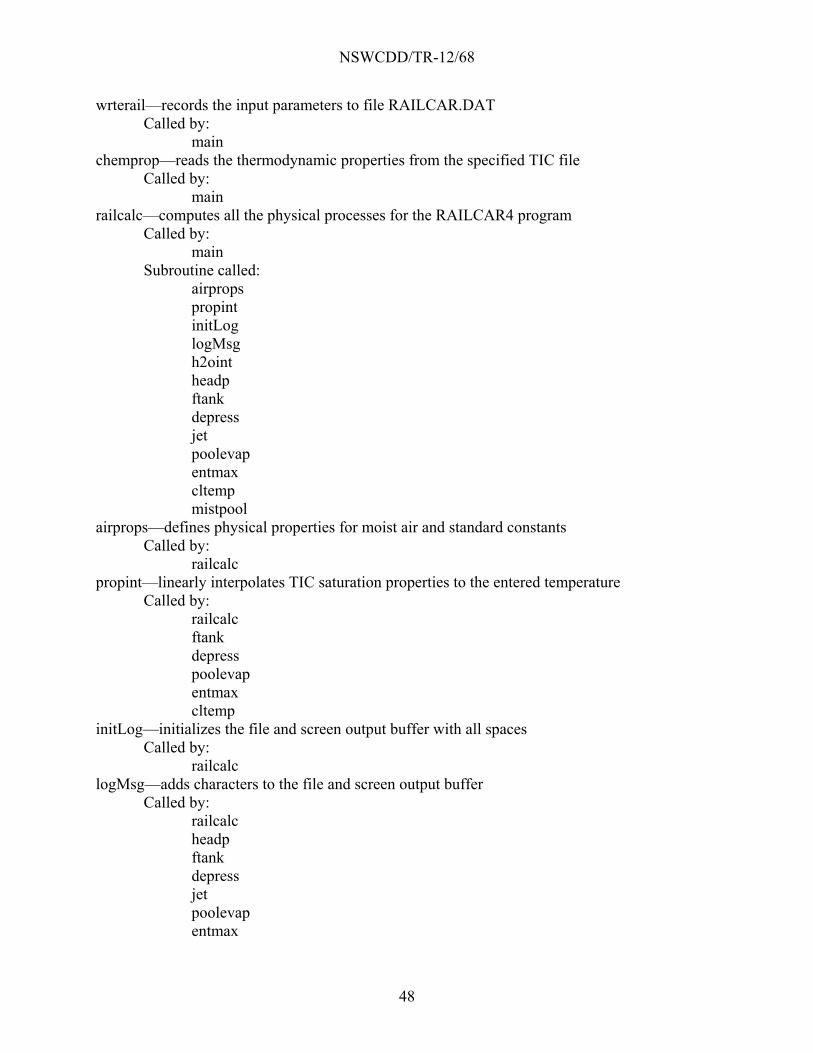
NSWCDD/TR-12/68

48

wrterail—records the input parameters to file RAILCAR.DAT Called by:

main chemprop—reads the thermodynamic properties from the specified TIC file

Called by: main railcalc—computes all the physical processes for the RAILCAR4 program

Called by: main

Subroutine called: airprops propint initLog logMsg h2oint headp ftank depress jet poolevap entmax cltemp mistpool airprops—defines physical properties for moist air and standard constants

Called by: railcalc propint—linearly interpolates TIC saturation properties to the entered temperature

Called by: railcalc ftank depress poolevap entmax cltemp initLog—initializes the file and screen output buffer with all spaces

Called by: railcalc logMsg—adds characters to the file and screen output buffer

Called by: railcalc headp ftank depress jet poolevap entmax

NSWCDD/TR-12/68

49

cltemp mistpool h2oint—defines and interpolates saturation properties for water to the entered temperature

Called by: railcalc entmax cltemp headp—calculates the liquid height and head pressure in the tank using a standard aspect ratio

Called by: railcalc

Subroutines called: logMsg ftank—calculates the temperature and masses in the tank after depressurization

Called by: railcalc

Subroutines called: logMsg expand propint expand—adiabatically expands vapor from one temperature and pressure to another

Called by: ftank depress—solves energy balances to determine the tank conditions when depressurization begins

Called by: railcalc

Subroutines called: propint logMsg jet—estimates initial and final liquid jet properties and initial vapor jet properties

Called by: railcalc

Subroutines called: logMsg poolevap—computes the vapor flux and diameter of a boiling or evaporating liquid pool

Called by: railcalc

Subroutines called: logMsg propint entmax—determines the maximum air entrainment ratio and cloud properties for aerosol survival

Called by: railcalc

Subroutines called: logMsg propint h2oint

NSWCDD/TR-12/68

50

cltemp—estimates the cloud properties after jet expansion and air entrainment Called by:

railcalc Subroutines called:

logMsg propint h2oint mistpool—determines if a mist pool will form and the subsequent cloud behavior

Called by: railcalc

Subroutines called: logMsg

NSWCDD/TR-12/68

51

4.0 CONCLUSIONS

NSWCDD is leading the way in improving hazard assessment modeling capabilities for TIC incidents. As a result of the validation of the NSWCDD mist pool theory, in conjunction with the extensive measurements taken during the Jack Rabbit pilot tests and field trials, hazard assessment models will be better equipped to predict the downwind effects for emergency responders, and warfighters will be much better protected from these types of attacks. The RAILCAR4 program provides the best source characterization for incidents involving release of pressurized liquids under low to moderate wind speeds, especially in the presence of buildings, vegetation, and/or terrain undulations. RAILCAR4 can be operated as a stand-alone program, or the calculations can be done from another program by calling the RAILCALC subroutine and providing the incident and chemical physical property parameters. Validation of the RAILCAR4 program with data from future field trials will provide confidence that the source characterization is accurate.

NSWCDD/TR-12/68

52

5.0 REFERENCES 1. Collision of Norfolk Southern Freight Train 192 with Standing Norfolk Southern Local

Train P22 with Subsequent Hazardous Materials Release at Graniteville, South Carolina, Railroad Accident Report, National Transportation Safety Board, NTSB/RAR-05/04, November 29, 2005.

2. Hanna, S. R., Comparisons of Six Models Using Three Chlorine Release Scenarios (Festus, Macdona, Graniteville), Hanna Consultants, Report Number P082, February 24, 2007.

3. Marshall, V. C., “The Predictions of Human Mortality from Chemical Accidents with Especial Reference to the Lethal Toxicity of Chlorine,” Journal of Hazardous Materials, 22 (1989), pp. 13-56.

4. Sharan, M., et. al., “Bhopal Gas Leak: A Numerical Simulation of Episodic Dispersion,” Atmospheric Environment, Vol. 29, No. 16, 1995, pp. 2061-2074.

5. “Toxic Industrial Hazard Source Term Characterization Technical Interchange Meeting,” Northrop Grumman, McLean, Virginia, November 8-9, 2006.

6. Goldwire, H. C., et al., Desert Tortoise Series Data Report, 1983 Pressurized Ammonia Spills, Lawrence Livermore National Laboratory, UCID-20562, December 1985.

7. Bauer, T., J., and Fox, S. B., “Characterization of the Initial Cloud of Chlorine Resulting from a 90-Ton Railcar Incident,” Department of Homeland Security, Chemical Security Analysis Center, September 2008.

8. Acute Exposure Guideline Levels for Selected Airborne Chemicals, Volume 2, The National Academies Press, 2002.

9. Witlox, H., and Harper, M., “PHAST Modeling for Liquid Chlorine Railcar Incidents,” DNV Software, Risk Management Solutions, 9 June 2007.

10. http://www.safersystem.com/pdfs/press/TRACE%20Version%209-1%20March07.pdf, TRACE, Version 9.1, Safer Systems, Camarillo, California, 13 March 2007.

11. Memorandum For Record #1, “TIC/TIM Task Force Prioritization & Application Recommendations,” Errata 1, 31 August 2009, which adopts Sutto, T. E., Toxic Industrial Chemicals: Global Assessment and Scientific Analysis, Naval Research Laboratory, District of Columbia, NRL\FR\6364--09-1,182, 2009.

NSWCDD/TR-12/68

53

12. “Naval Surface Warfare Center Dahlgren Division (NSWCDD) Statement of Work for Toxic Industrial Chemical (TIC) Railcar Incident Model Development,” U.S. Department of Homeland Security Science and Technology Directorate, HSHQDC-08-X-00498 SOW, June 2008.

13. Memorandum for Record #2A, “Emerging Priority TIC Operational Hazard Data, Applications and Preliminary Conclusions,” January 2010.

14. Toxic Industrial Chemical (TIC) Challenge Levels, DRAFT report for the NATO CSG, July 2010.

15. Wolski, M. G., “Threat Challenge Modeling (TCM) for the Joint Expeditionary Collective Protection (JECP) Family of Systems,” NSWCDD/TR-09/85, October 2009.

16. Investigation Report, Chlorine Release (66 Sought Medical Evaluation), U.S. Chemical Safety and Hazard Investigation Board, Report No. 2002-04-I-MO, May 2003.

17. Post, L., et al., HGSYSTEM 3.0: Technical Reference Manual and User's Guide, 1995.

18. A Dispersion Model for Elevated Dense Gas Jet Chemical Releases, Volume 1, EPA-450/4-88-006a, U.S. Environmental Protection Agency, Research Triangle Park, North Carolina, 1988.

19. A Dispersion Model for Elevated Dense Gas Jet Chemical Releases, Volume 2: Users Guide, EPA-450/4-88-006b, U.S. Environmental Protection Agency, Research Triangle Park, North Carolina, 1988.

20. Briggs, G. A., et al., “Dense Gas Vertical Diffusion Over Rough Surfaces: Results of Wind-Tunnel Studies,” Atmospheric Environment, 2001, 35, (13), pp. 2265-2284.

21. Goldwire, H. C., et al., Desert Tortoise Series Data Report, 1983 Pressurized Ammonia Spills, Lawrence Livermore National Laboratory, UCID-20562, December 1985.

22. Babarsky, R. J.; Sykes, R. I.; and Henn, D., “Chlorine Experiment/Model Comparison,” presentation to the 13th Annual George Mason University Conference, Fairfax, Virginia, July 2009.

23. http://www.defense.gov/news/newsarticle.aspx?id=46311

24. Storwald, D. P., Detailed Test Plan for the Jack Rabbit Test Program, U.S. Army Dugway Proving Ground, WDTC-TP-10-011, March 2010.

25. Vik, T., and Reif, B. A. P., Preliminary Assessment of the Vertical Release of Liquefied Chlorine Inside a Depression, FFI-rapport 2009/01251, Norwegian Defence Research Establishment (FFI), August 1, 2009.

26. “Ammonia: Large Scale Atmospheric Dispersion Tests,” INERIS Accidents Risk Division, Work Study No. 10072, December 2005.

NSWCDD/TR-12/68

54

27. webbook.nist.gov/chemistry/name-ser.html

28. The Merck Index, 9th Ed., Merck & Co., Inc., Rahway, New Jersey, 1976.

29. Reid, R.; Prausnitz, J.; and Poling, B., The Properties of Gases and Liquids, 4th Ed., McGraw-Hill Book Company, New York, 1987.

30. Perry, R., and Chilton, C., Chemical Engineers’ Handbook, 5th Ed., McGraw-Hill Book Company, New York, 1973.

31. Handbook of Chemistry and Physics, 62nd Ed., CRC Press, Inc., Boca Raton, Florida, 1981.

32. Dean, J., Lange’s Handbook of Chemistry, 13th Ed., McGraw-Hill Book Company, New York, 1985.

33. http://www.jtbaker.com/msds/english.html

34. http://www.puritanproducts.com/product_docs/ NITRIC%20ACID%20RED%20FUMING%20MSDS.pdf

35. Bauer, T., Software Design Description for the Chemical/Biological Agent Vapor, Liquid, and Solid Tracking (VLSTRACK) Computer Model, Version 3.0, NSWCDD/TR-98/6, December 1998.

NSWCDD/TR-12/68

(1)

DISTRIBUTION

Copies

DOD ACTIVITIES (CONUS) DEFENSE TECH INFORMATION CTR 2 8725 JOHN J KINGMAN RD SUITE 0944 FORT BELVOIR VA 22060-6218 NON-DOD ACTIVITIES (CONUS) ATTN DOCUMENT CENTER 1 THE CNA CORPORATION 4825 MARK CENTER DRIVE ALEXANDRIA VA 22311-1850 ATTN JOHN CHIN 4 GOVERNMENT DOCUMENTS SECTION 101 INDEPENDENCE AVENUE SE LIBRARY OF CONGRESS WASHINGTON DC 20540-4172

Copies

INTERNAL CX7 (TECHNICAL LIBRARY) 2 Z24 (DAVE) 1 Z24 (BAUER) 1 G32 (VAN BUREN) 1