DAA Unit III Backtracking and Branch and Bound · By Prof. B.A.Khivsara Assistant Professor...
67
By Prof. B.A.Khivsara Assistant Professor Department of Computer Engineering SNJB’s KBJ COE, Chandwad DAA Unit III Backtracking and Branch and Bound
Transcript of DAA Unit III Backtracking and Branch and Bound · By Prof. B.A.Khivsara Assistant Professor...

By Prof. B.A.Khivsara
Assistant Professor
Department of Computer Engineering
SNJB’s KBJ COE, Chandwad
DAA Unit III
Backtracking and Branch and Bound
Backtracking
3
BACKTRACKING
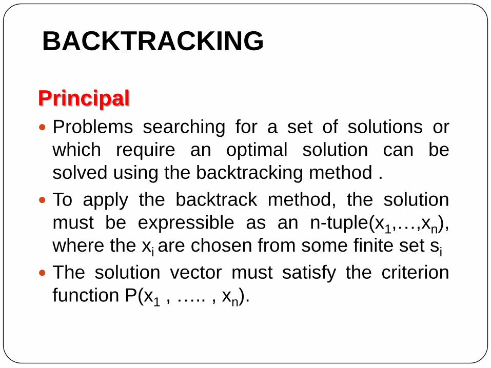
Principal
Problems searching for a set of solutions or
which require an optimal solution can be
solved using the backtracking method .
To apply the backtrack method, the solution
must be expressible as an n-tuple(x1,…,xn),
where the xi are chosen from some finite set si
The solution vector must satisfy the criterion
function P(x1 , ….. , xn).
4
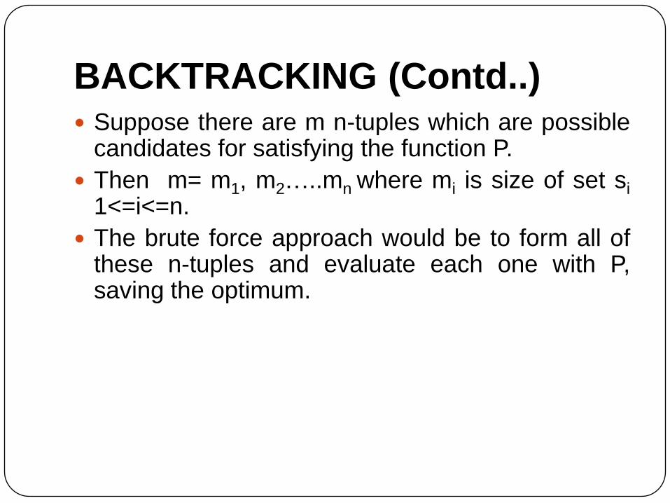
BACKTRACKING (Contd..) Suppose there are m n-tuples which are possible
candidates for satisfying the function P.
Then m= m1, m2…..mn where mi is size of set si
1<=i<=n.
The brute force approach would be to form all ofthese n-tuples and evaluate each one with P,saving the optimum.

5
BACKTRACKING (Contd..)
The backtracking algorithm has the ability to yield
the same answer with far fewer than m-trials.
In backtracking, the solution is built one
component at a time.
Modified criterion functions Pi (x1...xn) called
bounding functions are used to test whether the
partial vector (x1,x2,......,xi) can lead to an optimal
solution.
If (x1,...xi) is not leading to a solution, mi+1,....,mn
possible test vectors may be ignored.
6
BACKTRACKING – Constraints
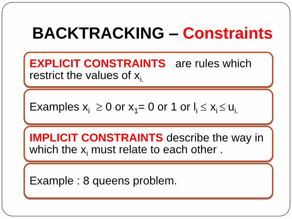
EXPLICIT CONSTRAINTS are rules which restrict the values of xi.
Examples xi 0 or x1= 0 or 1 or li xi ui.
IMPLICIT CONSTRAINTS describe the way in which the xi must relate to each other .
Example : 8 queens problem.

7
BACKTRACKING: Solution Space
Tuples that satisfy the explicit constraints define a solution space.
The solution space can be organized into a tree.
Each node in the tree defines a problem state.
All paths from the root to other nodes define the state-space of the problem.
Solution states are those states leading to a tuple in the solution space.
Answer nodes are those solution states leading to an answer-tuple( i.e. tuples which satisfy implicit constraints).

8
BACKTRACKING -Terminology
LIVE NODE A node which has been generated and all of whose children are not yet been generated .
E-NODE (Node being expanded) - The live node whose children are currently being generated .
DEAD NODE - A node that is either not to be expanded further, or for which all of its children have been generated
DEPTH FIRST NODE GENERATION- In this, as soon as a new child C of the current E-node R is generated, C will become the new E-node.

9
BACKTRACKING -Terminology
BOUNDING FUNCTION - will be used to kill live nodes without generating all their children.
BACTRACKING-is depth – first node generation with bounding functions.
BRANCH-and-BOUND is a method in which E-node remains E-node until it is dead.

10
BACKTRACKING -Terminology
BREADTH-FIRST-SEARCH : Branch-and Bound with each new node placed in a queue .The front of the queen becomes the new E-node.
DEPTH-SEARCH (D-Search) : New nodes are placed in to a stack.The last node added is the first to be explored.

11
BACKTRACKING (4 Queens problem)
Example :
1
. . 2
1
2
1
2
3
. . . .
1
1 1
2
3
. , 4

12
BACKTRACKING (Contd..)
We start with root node as the only live node.
The path is ( ); we generate a child node 2.
The path is (1).This corresponds to placing
queen 1 on column 1 .
Node 2 becomes the E node. Node 3 is
generated and immediately killed. (because
x1=1,x2=2).
As node 3 is killed, nodes 4,5,6,7 need not be
generated.

13
Iterative Control Abstraction
( General Backtracking Method)
Procedure Backtrack(n)
{ K 1
while K > 0 do
if there remained an untried X(K) such that X(K)
T ( X (1) , …..X(k-1) ) and Bk X (1) ,…,X(K) ) = true then
if (X (1),…, X(k) ) is a path to an answer node then
print ( X (1) ,…X (k) )
end if
K K+1 // consider next set //
else K K-1 // backtrack to previous set
endif
repeat
end Backtrack
}

14
RECURSION Control Abstraction
( General Backtracking Method)
Procedure RBACKTRACK (k)
{ Global n , X(1:n)
for each X(k) such that
X(k) T ( X (1),..X(k-1) ) and Bk (X(1)..,X(k-1), X(k) )= true do
if ( X (1) ,….,X(k) ) is a path to an answer node
then print ( X(1),……,X(k) ) end if
If (k<n)
CALL RBACKTRACK (k+1)
endif
repeat
End RBACKTRACK
}

15
EFFICIENCY OF BACKTRACKING
ALGORITHM Depend on 4 Factors
• The time to generate the next X(k)
The no. of X(k) satisfying the
explicit constraints
The time for bounding
functions Bi
The no. of X(k) satisfying the Bi for all i

N queens problem
using Backtracking

17
The n-queens problem and solution
In implementing the n – queens problem weimagine the chessboard as a two-dimensionalarray A (1 : n, 1 : n).
The condition to test whether two queens, atpositions (i, j) and (k, l) are on the same rowor column is simply to check I = k or j = l
The conditions to test whether two queens areon the same diagonal or not are to be found

18
The n-queens problem and solution
contd..
Observe that
i) For the elements in the
the upper left to lower
Right diagonal, the row -
column values are same
or row- column = 0,
e.g. 1-1=2-2=3-3=4-4=0
ii) For the elements in the upper right to the lower left diagonal, row + column value is the same e.g. 1+4=2+3=3+2=4+1=5
(1,1) (1,2) (1,3) (1,4)
(2,1) (2,2) (2,3) (2,4)
(3,1) (3,2) (3,3) (3,4)
(4,1) (4,2) (4,3) (4,4)
19
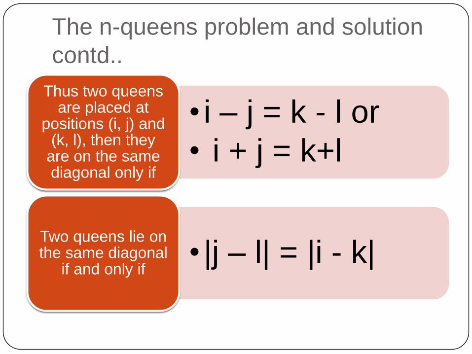
The n-queens problem and solution
contd..
• i – j = k - l or
• i + j = k+l
Thus two queens are placed at
positions (i, j) and (k, l), then they
are on the same diagonal only if
• |j – l| = |i - k| Two queens lie on the same diagonal
if and only if

20
The n-queens problem -Algorithm
Procedure PLACE (k) {
for i 1 to k-1 do
if X(i) = X(k) // two are in the same column
or ABS(X(i) –X(k)) = ABS(i-k) // in the same diagonal
then Return (false)
end if
repeat
return (true)
end
}

21
The n-queens problem -Algorithm contd..
Procedure N queens(n)
{ X(1) 0 ; k1 // k is the current row,//
while k > 0 do
X(k) X(k) + 1
While X(k) n and not PLACE(k)
X(k) X(k) + 1
repeat
if X(k) n then
if k = n then print(X)
else k k+1;
X(k) = 0
endif
else k k-1
endif
repeat
end NQUEENS

Graph Coloring Problem
using Backtracking

23
GRAPH COLOURING PROBLEM
Let G be a graph and m be a positive integer .
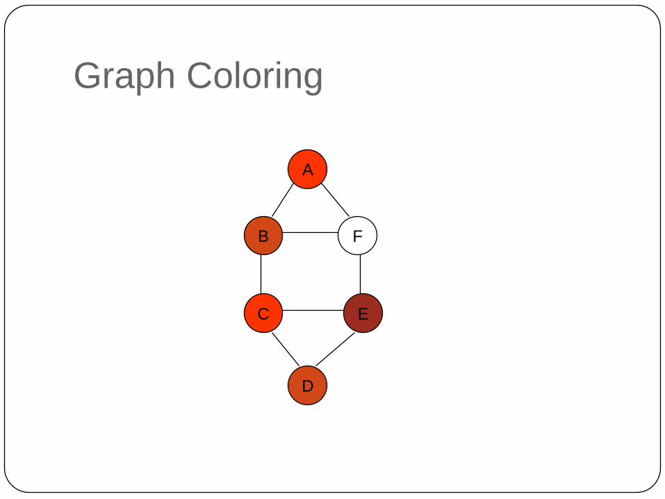
The problem is to color the vertices of G using only m colors in such a way that no two adjacent nodes / vertices have the same color.
It is necessary to find the smallest integer m. m is referred to as the chromatic number of G.

24
GRAPH COLOURING PROBLEM (Contd..)
A map can be transformed into a graph by representing each region of map into a node and if two regions are adjacent, then the corresponding nodes are joined by an edge.
For many years it was known that 5 colors are required to color any map.
After a several hundred years, mathematicians with the help of a computer showed that 4 colours are sufficient.
25
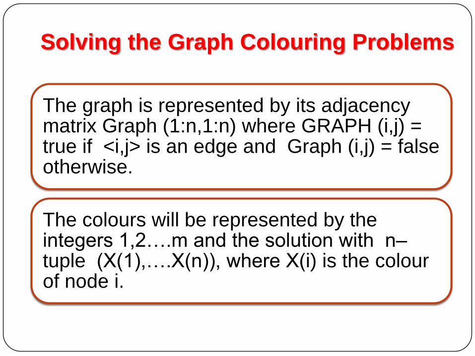
Solving the Graph Colouring Problems
The graph is represented by its adjacency matrix Graph (1:n,1:n) where GRAPH (i,j) = true if <i,j> is an edge and Graph (i,j) = false otherwise.
The colours will be represented by the integers 1,2….m and the solution with n–tuple (X(1),….X(n)), where X(i) is the colourof node i.

26
Solving the Graph Colouring Problems
(Contd..)
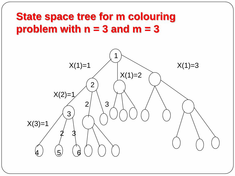
The solution can be represented as a state space tree.
Each node at level i has m children corresponding to m possible assignments to X(i) 1≤i≤m.
Nodes at level n+1, are leaf nodes. The tree has degree m with height n+1.
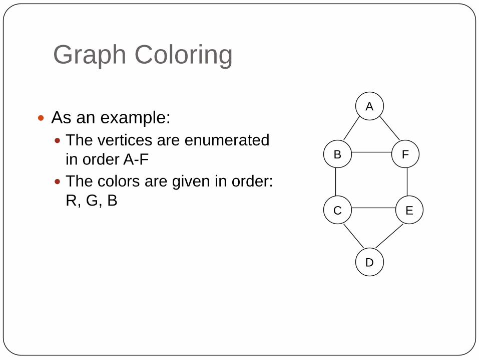
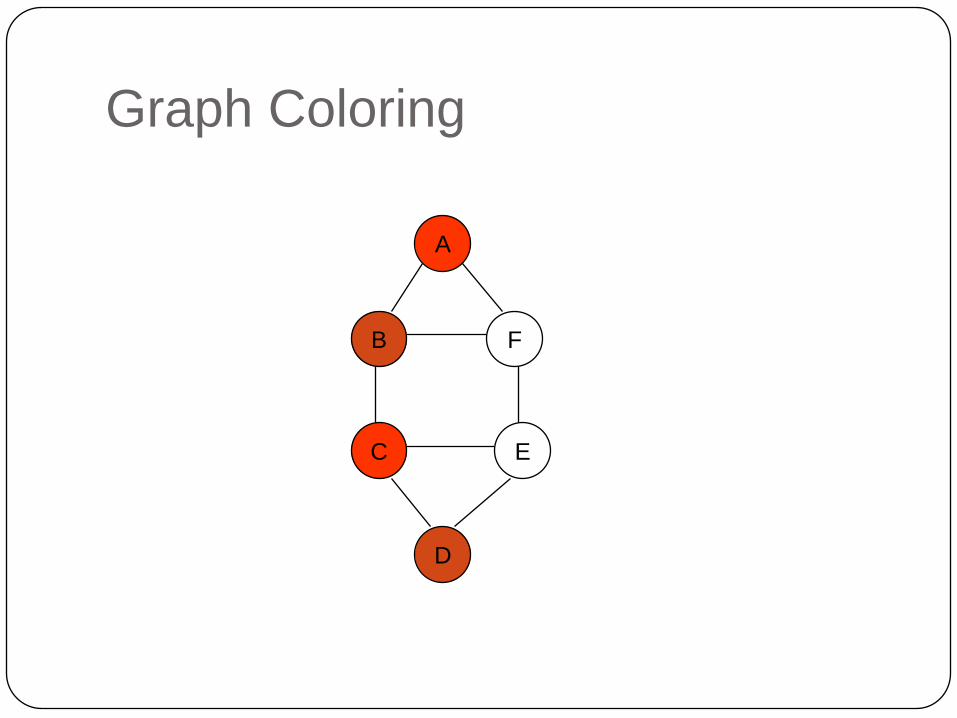
Graph Coloring
C
A
FB
E
D
As an example:
The vertices are enumerated
in order A-F
The colors are given in order:
R, G, B

Graph Coloring
C
A
FB
E
D

Graph Coloring
C
A
FB
E
D

Graph Coloring
C
A
FB
E
D
Graph Coloring
C
A
FB
E
D
Graph Coloring
C
A
FB
E
D

Graph Coloring
C
A
FB
E
D

Graph Coloring
C
A
FB
E
D

Graph Coloring
C
A
FB
E
D

Graph Coloring
C
A
FB
E
D

Graph Coloring
C
A
FB
E
D

Graph Coloring
C
A
FB
E
D
39
State space tree for m colouring
problem with n = 3 and m = 3
1
X(1)=1 X(1)=3
X(1)=2
2
X(2)=1
2 3
3
X(3)=1
2 3
4 5 6
40
Graph Colouring Problem- Algorithm
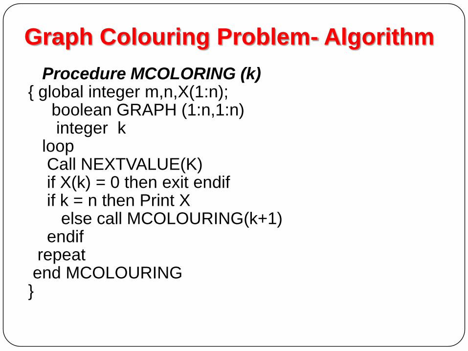
Procedure MCOLORING (k){ global integer m,n,X(1:n);
boolean GRAPH (1:n,1:n)integer k
loopCall NEXTVALUE(K) if X(k) = 0 then exit endifif k = n then Print X
else call MCOLOURING(k+1)endif
repeat end MCOLOURING }

41
Graph Colouring Problem- Algorithm
(Cont…)
Procedure NEXTVALUE(k)
{
Repeat
{
X(k)( X(k) +1 ) mod(m+1)
if X(k)=0 then return endif
for j 1 to n doif GRAPH(k,j) and X(k)=X(j) then exit endifif j = n+1 then return endif
} Until(False)}

Sum of Subset Problem
using Backtracking
Sum-of-Subsets problem
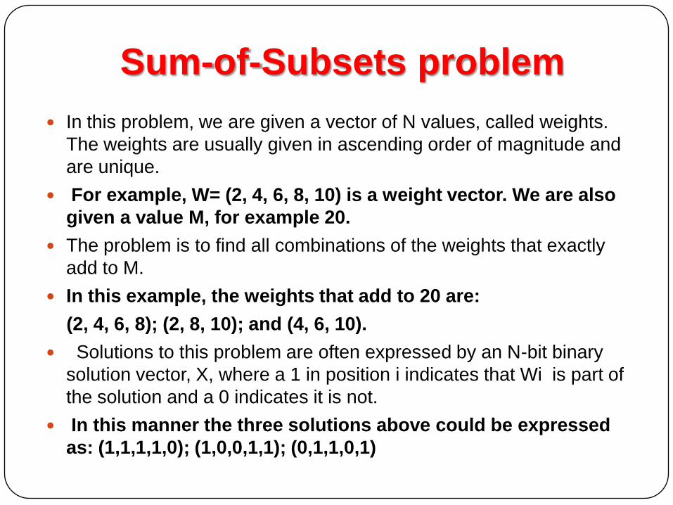
In this problem, we are given a vector of N values, called weights.
The weights are usually given in ascending order of magnitude and
are unique.
For example, W= (2, 4, 6, 8, 10) is a weight vector. We are also
given a value M, for example 20.
The problem is to find all combinations of the weights that exactly
add to M.
In this example, the weights that add to 20 are:
(2, 4, 6, 8); (2, 8, 10); and (4, 6, 10).
Solutions to this problem are often expressed by an N-bit binary
solution vector, X, where a 1 in position i indicates that Wi is part of
the solution and a 0 indicates it is not.
In this manner the three solutions above could be expressed
as: (1,1,1,1,0); (1,0,0,1,1); (0,1,1,0,1)
Sum-of-Subsets problem
We are given ‘n’ positive numbers called weights and we have to find all combinations of these numbers whose sum is M. this is called sum of subsets problem.
If we consider backtracking procedure using fixed tuple strategy , the elements X(i) of the solution vector is either 1 or 0 depending on if the weight W(i) is included or not.
If the state space tree of the solution, for a node at level I, the left child corresponds to X(i)=1 and right to X(i)=0.

Sum of Subsets Algorithmvoid SumOfSub(float s, int k, float r)
{
// Generate left child.
x[k] = 1;
if (s+w[k] == m)
{ for (int j=1; j<=k; j++)
Print (x[j] )
}
else if (s+w[k]+w[k+1] <= m)
SumOfSub(s+w[k], k+1, r-w[k]);
// Generate right child and evaluate
if ((s+r-w[k] >= m) && (s+w[k+1] <= m)) {
x[k] = 0;
SumOfSub(s, k+1, r-w[k]);
}
}

Sum of Subsets State Space Tree Example n=6, w[1:6]={5,10,12,13,15,18}, m=30

Branch and Bound

Branch and Bound Principal
The term branch-and-bound refers to all state space search methods in which all children of the £-node are generated before any other live node can become the £-node.
We have already seen two graph search strategies, BFS and D-search, in which the exploration of a new node cannot begin until the node currently being explored is fully explored.
Both of these generalize to branch-and-bound strategies.
In branch-and-bound terminology, a BFS-like state space search will be called FIFO (First In First Out) search as the list of live nodes is a first-in-first-out list (or queue).
A D-searchlike state space search will be called LIFO (Last In First Out) search as the list of live nodes is a last-in-first-out list (or stack).

Control Abstraction for Branch
and Bound(LC Method)
LC Method Control Abstarction
Explanation
The search for an answer node can often be
speeded by using an "intelligent" ranking function,
c(. ), for live nodes.
The next £-node is selected on the basis of this
ranking function.
Let T be a state space tree and c( ) a cost
function for the nodes in T. If X is a node in T then
c(X) is the minimum cost of any answer node in
the subtree with root X. Thus, c(T) is the cost of a
minimum cost answer node

LC Method Control Abstarction
Explanation
The algorithm uses two subalgorithms LEAST(X)
and ADD(X) to respectively delete and add a live
node from or to the list of live nodes.
LEAST{X) finds a live node with least c( ). This
node is deleted from the list of live nodes and
returned in variable X.
ADD(X) adds the new live node X to the list of
live nodes.
Procedure LC outputs the path from the answer
node it finds to the root node T.

0/1 knapsack problem using
Branch and Bound
53
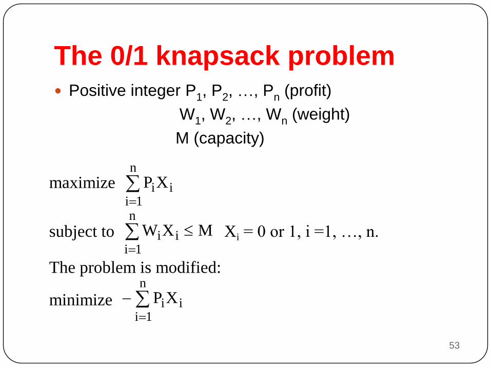
The 0/1 knapsack problem Positive integer P1, P2, …, Pn (profit)
W1, W2, …, Wn (weight)
M (capacity)
maximize P Xi ii
n
1
subject to W X Mi ii
n
1
Xi = 0 or 1, i =1, …, n.
The problem is modified:
minimize
P Xi ii
n
1

54
The 0/1 knapsack problem
The Branching Mechanism in the Branch-and-Bound Strategy to
Solve 0/1 Knapsack Problem.
55
How to find the upper bound?
Ans: by quickly finding a feasible solution in a
greedy manner: starting from the smallest
available i, scanning towards the largest i’s until
M is exceeded. The upper bound can be
calculated.

56
How to find the ranking Function
Ans: by relaxing our restriction from Xi = 0 or 1 to
0 Xi 1 (knapsack problem)
Let
P Xi ii
n
1
be an optimal solution for 0/1
knapsack problem and
P Xii
n
i1
be an optimal
solution for fractional knapsack problem. Let
Y=
P Xi ii
n
1
, Y’ =
P Xii
n
i1
.
Y’ Y
57
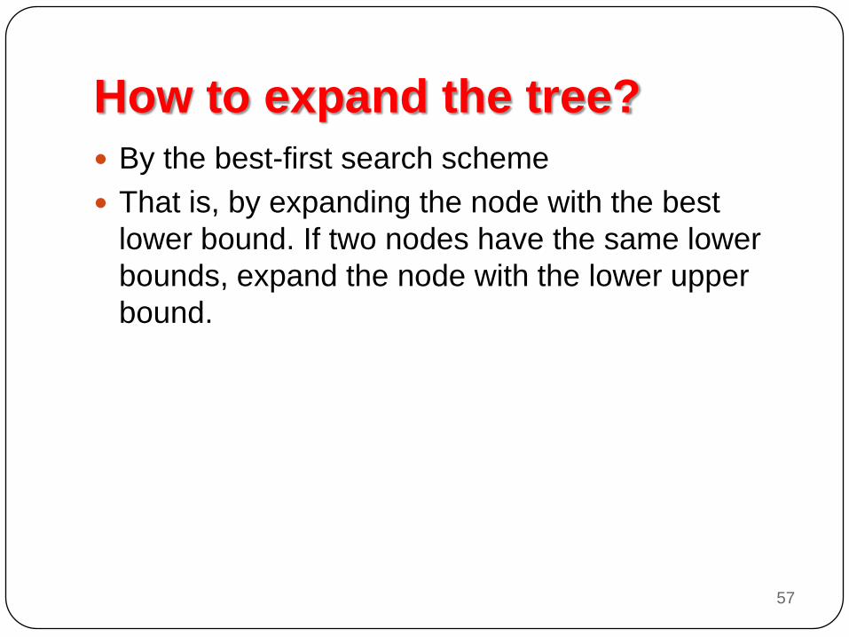
How to expand the tree?
By the best-first search scheme
That is, by expanding the node with the best
lower bound. If two nodes have the same lower
bounds, expand the node with the lower upper
bound.

0/1 Knapsack algorithm using BB

0/1 Knapsack Example using
LCBB (Least Cost)
Example (LCBB)
Consider the knapsack instance:
n = 4;
(pi, p2,
p3, p4) = (10, 10, 12, 18);
(wi. w2, w3, w4) = (2, 4, 6, 9) and
M = 15.

0/1 Knapsack State Space tree of
Example using LCBB
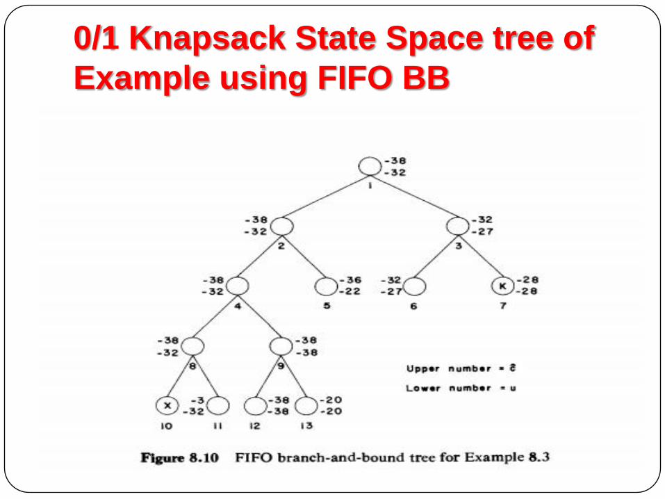
0/1 Knapsack State Space tree of
Example using FIFO BB

Traveling Salesman problem (TSP)
using Branch and Bound

63
The traveling salesperson problem
Given a graph, the TSP Optimization problem
is to find a tour, starting from any vertex,
visiting every other vertex and returning to the
starting vertex, with minimal cost.

64
The basic idea
There is a way to split the solution space
(branch)
There is a way to predict a lower bound for a
class of solutions. There is also a way to find
a upper bound of an optimal solution. If the
lower bound of a solution exceeds the upper
bound, this solution cannot be optimal and
thus we should terminate the branching
associated with this solution.

Example- TSP
Example with Cost
Matrix(a) and its
Reduced Cost Matrix (b)
Reduced matrix means
every row and column of
matrix should contain at
least one Zero and all
other entries should be
non negative.

Reduced Matrix for node 2,3…10 of
State Space tree using LC Method
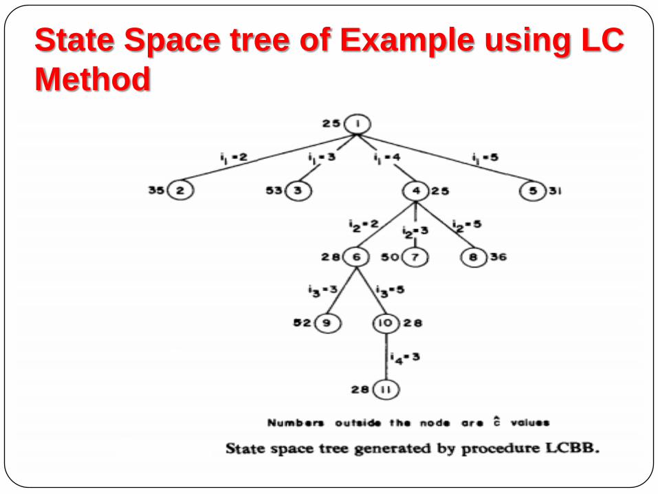
State Space tree of Example using LC
Method