
DAA unit 7 Branch and Boundmpesguntur.com/PDF/NOTES/CSE/DAA/DAA_unit_7_Branch and...Dr.DSK III CSE--...
22
Dr.DSK III CSE-- DAA UNIT-VII Branch and Bound Page 1 DESIGN AND ANALYSIS OF ALGORITHMS UNIT-VII – BRANCH AND BOUND Branch and Bound: General method, Applications- Travelling salesperson problem, 0/1 Knapsack problem- LC Branch and Bound solution, FIFO Branch and bound solution. -0-0-0-0- Introduction: The term Branch and Bound refers to all state space search methods in which all children of the E-Node are generated before any other live node can become the E-Node. We have already seen two graph search strategies, BFS and DFS in which the exploration of a new node cannot begin until the node currently being explored is fully explored. Both of these generalize to Branch and Bound strategies. In Branch and Bound BFS like space search will be called FIFO search as the list of live nodes is a first in first out list (or queue). A DFS like state space search will be called LIFO (Last In First Out) search as the list of live nodes is a last in first out list (or Stack). Ex) let us see how a FIFO branch and bound algorithm would search the state space tree for the 4 queens problem. We have already solved the problem using backtracking as under. Fig 1) state space tree for 4 queens problem. Nodes are numbered in DFS
Transcript of DAA unit 7 Branch and Boundmpesguntur.com/PDF/NOTES/CSE/DAA/DAA_unit_7_Branch and...Dr.DSK III CSE--...

Dr.DSK III CSE-- DAA UNIT-VII Branch and Bound Page 1
DESIGN AND ANALYSIS OF ALGORITHMS
UNIT-VII – BRANCH AND BOUND
Branch and Bound: General method, Applications- Travelling
salesperson problem, 0/1 Knapsack problem- LC Branch and Bound
solution, FIFO Branch and bound solution.
-0-0-0-0-
Introduction:
The term Branch and Bound refers to all state space search
methods in which all children of the E-Node are generated
before any other live node can become the E-Node.
We have already seen two graph search strategies, BFS and DFS
in which the exploration of a new node cannot begin until the
node currently being explored is fully explored.
Both of these generalize to Branch and Bound strategies.
In Branch and Bound BFS like space search will be called FIFO
search as the list of live nodes is a first in first out list
(or queue).
A DFS like state space search will be called LIFO (Last In
First Out) search as the list of live nodes is a last in first
out list (or Stack).
Ex) let us see how a FIFO branch and bound algorithm would
search the state space tree for the 4 queens problem. We have
already solved the problem using backtracking as under.
Fig 1) state space tree for 4 queens problem. Nodes are
numbered in DFS
Dr.DSK III CSE-- DAA UNIT-VII Branch and Bound Page 2
Some terminology regarding tree organizations of solution
spaces.
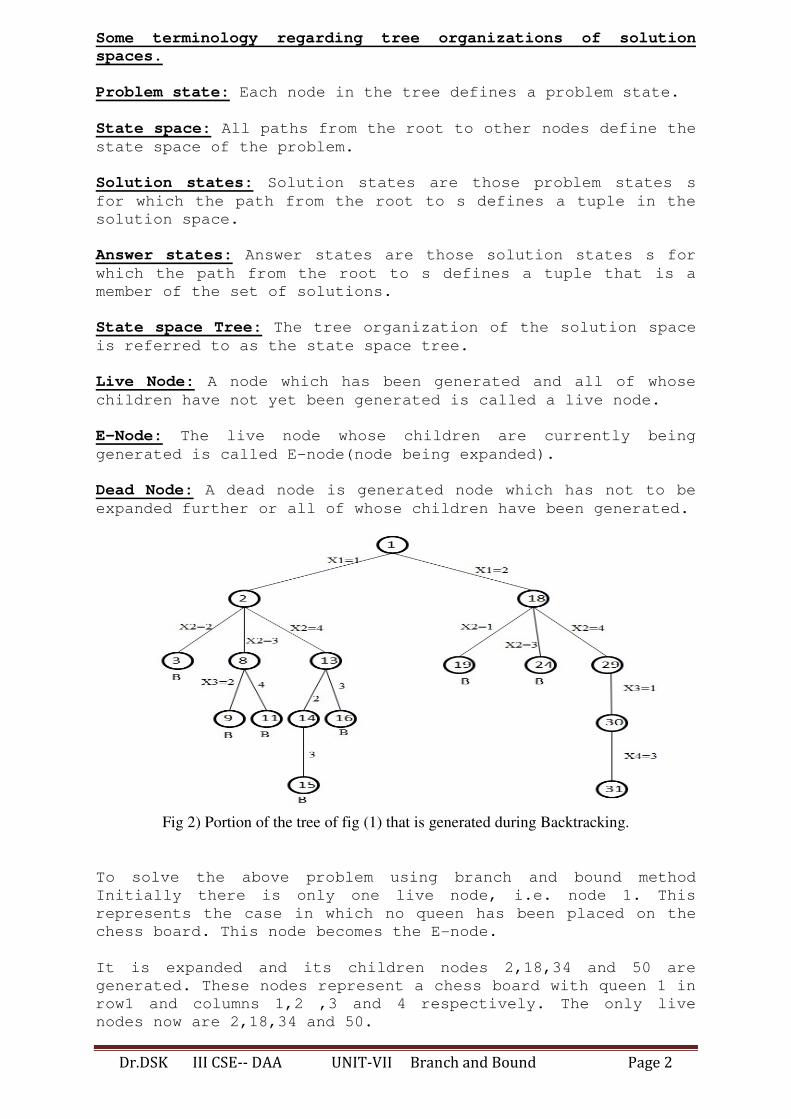
Problem state: Each node in the tree defines a problem state.
State space: All paths from the root to other nodes define the
state space of the problem.
Solution states: Solution states are those problem states s
for which the path from the root to s defines a tuple in the
solution space.
Answer states: Answer states are those solution states s for
which the path from the root to s defines a tuple that is a
member of the set of solutions.
State space Tree: The tree organization of the solution space
is referred to as the state space tree.
Live Node: A node which has been generated and all of whose
children have not yet been generated is called a live node.
E-Node: The live node whose children are currently being
generated is called E-node(node being expanded).
Dead Node: A dead node is generated node which has not to be
expanded further or all of whose children have been generated.
Fig 2) Portion of the tree of fig (1) that is generated during Backtracking.
To solve the above problem using branch and bound method
Initially there is only one live node, i.e. node 1. This
represents the case in which no queen has been placed on the
chess board. This node becomes the E-node.
It is expanded and its children nodes 2,18,34 and 50 are
generated. These nodes represent a chess board with queen 1 in
row1 and columns 1,2 ,3 and 4 respectively. The only live
nodes now are 2,18,34 and 50.
Dr.DSK III CSE-- DAA UNIT-VII Branch and Bound Page 3
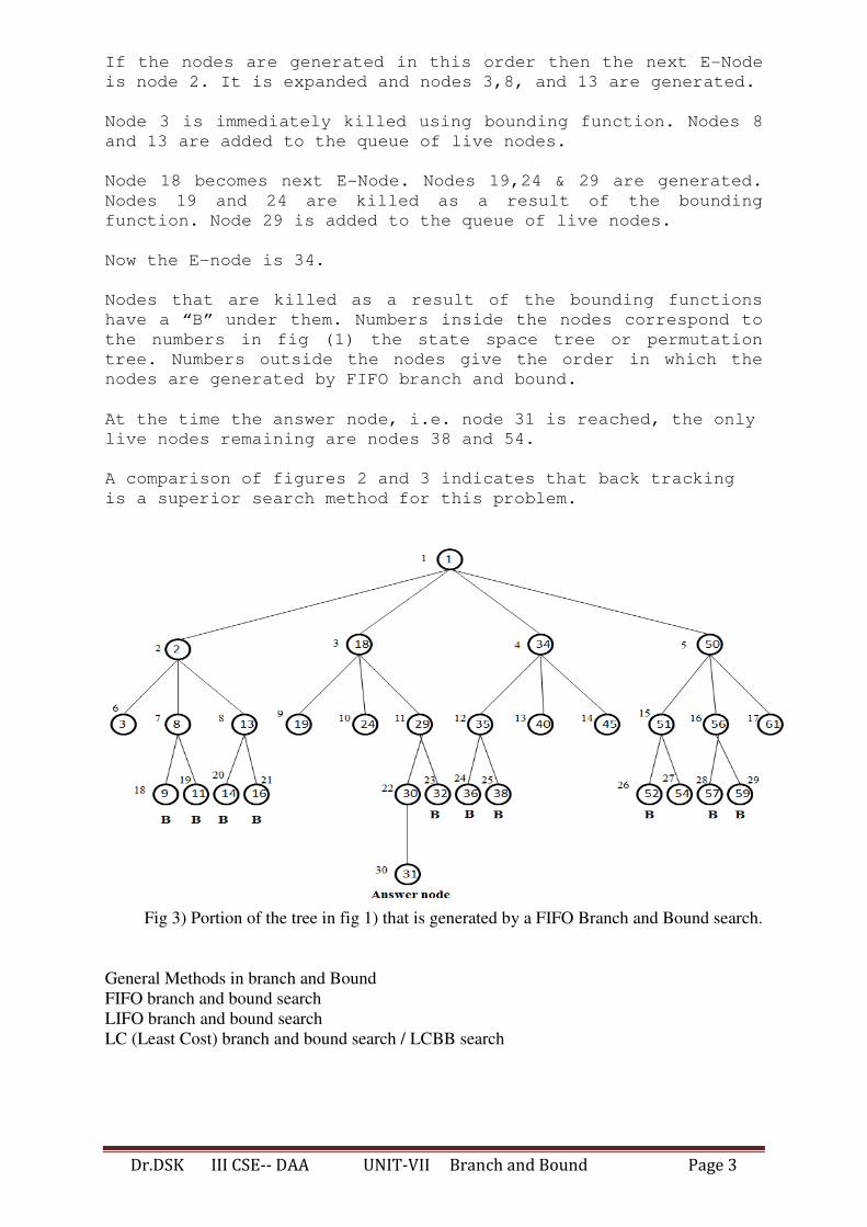
If the nodes are generated in this order then the next E-Node
is node 2. It is expanded and nodes 3,8, and 13 are generated.
Node 3 is immediately killed using bounding function. Nodes 8
and 13 are added to the queue of live nodes.
Node 18 becomes next E-Node. Nodes 19,24 & 29 are generated.
Nodes 19 and 24 are killed as a result of the bounding
function. Node 29 is added to the queue of live nodes.
Now the E-node is 34.
Nodes that are killed as a result of the bounding functions
have a “B” under them. Numbers inside the nodes correspond to
the numbers in fig (1) the state space tree or permutation
tree. Numbers outside the nodes give the order in which the
nodes are generated by FIFO branch and bound.
At the time the answer node, i.e. node 31 is reached, the only
live nodes remaining are nodes 38 and 54.
A comparison of figures 2 and 3 indicates that back tracking
is a superior search method for this problem.
Fig 3) Portion of the tree in fig 1) that is generated by a FIFO Branch and Bound search.
General Methods in branch and Bound
FIFO branch and bound search
LIFO branch and bound search
LC (Least Cost) branch and bound search / LCBB search
Dr.DSK III CSE-- DAA UNIT-VII Branch and Bound Page 4
FIFO branch and bound search
Fig 4) State space tree
Assume that the node 12 is an answer node (solution).
In FIFO search first we start with node 1. i.e. E-Node is 1.
Next we generate the children of node 1. We place all the live nodes in queue
2 3 4
Now we delete an element from queue i.e. node 2, next and node 2 becomes E-node and
generates its children and places those live nodes in queue.
3 4 5 6
Next, delete an element from queue and considering it as E-node. i.e. E-node =3 and its
children are generated. 7,8 are children of 3 and these live nodes are killed by bounding
functions. So we will not include in queue.
4 5 6
Again delete an element from Q. considering it as E-node, generate the children of node 4.
Node 9 is generated and killed by bounding function.
5 6
Again delete an element from Q. generate children of node 5, i.e. nodes 10 and 11 are
generated and killed by bounding function, last node in the queue is 6.
6
The child of node 6 is 12 and it satisfies the conditions of the problem which is the answer
node, so search terminates.
LIFO branch and bound search
Fig 5) State space tree
For LIFO branch and bound we use the data structure stack. Initially stack is empty.
The order is 1,2,5,10,11,6,12
10 top
5
2
1
stack

Dr.DSK III CSE-- DAA UNIT-VII Branch and Bound Page 5
LC (Least Cost) branch and bound search / LCBB search
In this we use a ranking function or cost function, which is denoted by ˆ( )c x . We generate the
children of the E-node, among these live nodes, we select a node which has minimum cost.
By using the ranking function we will calculate the cost of each node.
Note that the ranking function ˆ( )c x or cost function which depends on the problem.
Initially we take the node 1 as E-node.
Generate children of node 1, the children are 2,3,and 4. By using the ranking function we
calculate the cost of 2,3 and 4 nodes as ˆ(2) 2c = , ˆ(3) 3c = , ˆ(4) 4c = .Now we select a node
which has minimum cost i.e. node 2. For node 2 the children are 5 and 6. ˆ(5) 4c = , ˆ(6) 1c = we
select node 6 as cost is less. Generate children of 6 i.e. 12 and 13. We select node 12 since its
cost is 1 i.e. minimum. More over node 12 is the answer node. So we terminate search
process.
Fig 6) State space tree
Applications
Travelling salesperson problem :: LCBB Solution
0/1 Knapsack problem :: LCBB solution
0/1 Knapsack problem :: FIFOBB solution
Dr.DSK III CSE-- DAA UNIT-VII Branch and Bound Page 6
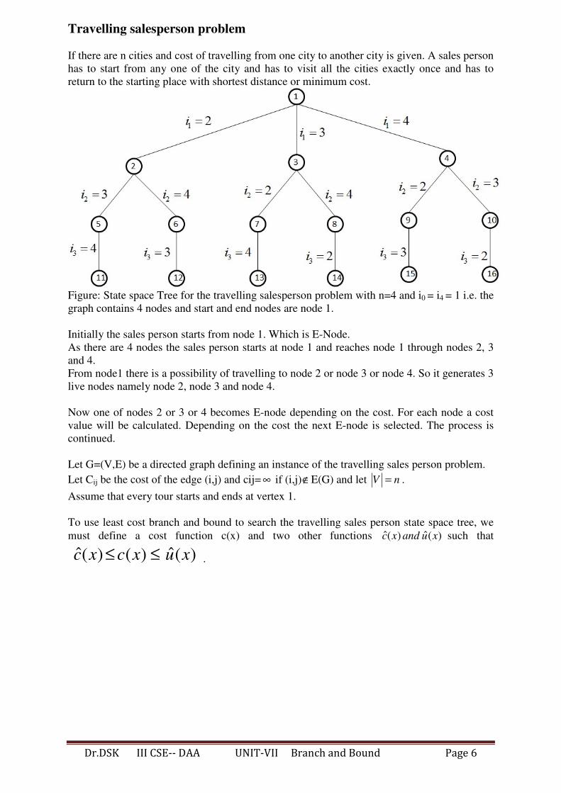
Travelling salesperson problem
If there are n cities and cost of travelling from one city to another city is given. A sales person
has to start from any one of the city and has to visit all the cities exactly once and has to
return to the starting place with shortest distance or minimum cost.
Figure: State space Tree for the travelling salesperson problem with n=4 and i0 = i4 = 1 i.e. the
graph contains 4 nodes and start and end nodes are node 1.
Initially the sales person starts from node 1. Which is E-Node.
As there are 4 nodes the sales person starts at node 1 and reaches node 1 through nodes 2, 3
and 4.
From node1 there is a possibility of travelling to node 2 or node 3 or node 4. So it generates 3
live nodes namely node 2, node 3 and node 4.
Now one of nodes 2 or 3 or 4 becomes E-node depending on the cost. For each node a cost
value will be calculated. Depending on the cost the next E-node is selected. The process is
continued.
Let G=(V,E) be a directed graph defining an instance of the travelling sales person problem.
Let Cij be the cost of the edge (i,j) and cij= ∞ if (i,j)∉E(G) and let V n= .
Assume that every tour starts and ends at vertex 1.
To use least cost branch and bound to search the travelling sales person state space tree, we
must define a cost function c(x) and two other functions ˆ ˆ( ) ( )c x and u x such that
ˆ ˆ( ) ( ) ( )c x c x u x≤ ≤ .
Dr.DSK III CSE-- DAA UNIT-VII Branch and Bound Page 7
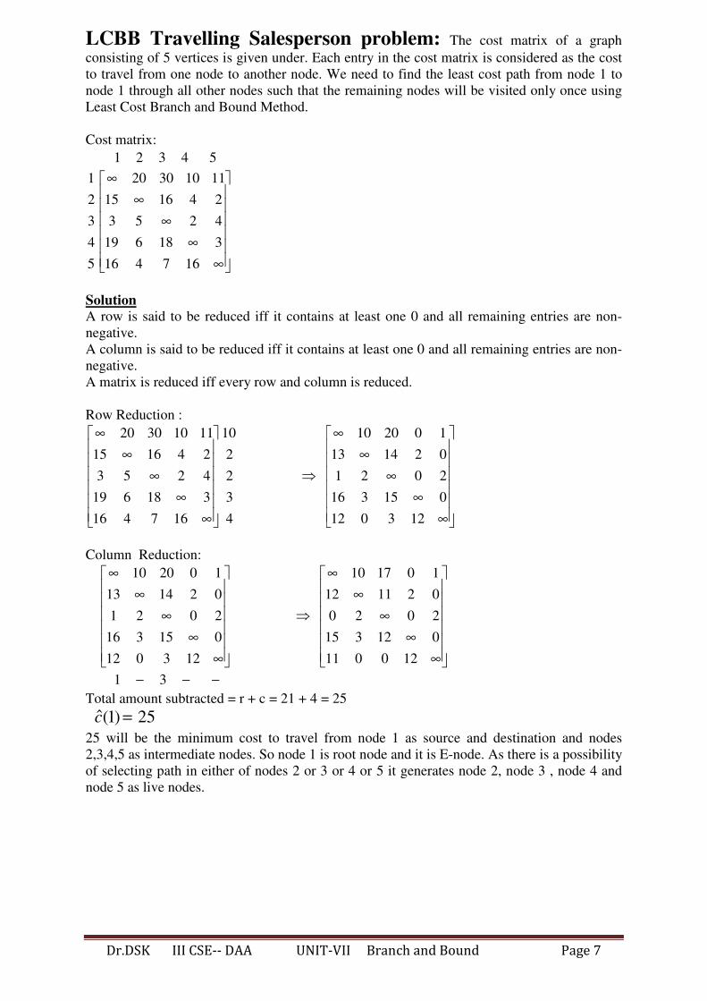
LCBB Travelling Salesperson problem: The cost matrix of a graph
consisting of 5 vertices is given under. Each entry in the cost matrix is considered as the cost
to travel from one node to another node. We need to find the least cost path from node 1 to
node 1 through all other nodes such that the remaining nodes will be visited only once using
Least Cost Branch and Bound Method.
Cost matrix:
1 2 3 4 5
1
2
3
4
5
20 30 10 11
15 16 4 2
3 5 2 4
19 6 18 3
16 4 7 16
∞
∞ ∞
∞
∞
Solution
A row is said to be reduced iff it contains at least one 0 and all remaining entries are non-
negative.
A column is said to be reduced iff it contains at least one 0 and all remaining entries are non-
negative.
A matrix is reduced iff every row and column is reduced.
Row Reduction :
20 30 10 11
15 16 4 2
3 5 2 4
19 6 18 3
16 4 7 16
∞
∞ ∞
∞
∞
10
2
2
3
4
10 20 0 1
13 14 2 0
1 2 0 2
16 3 15 0
12 0 3 12
∞
∞ ⇒ ∞
∞
∞
Column Reduction:
10 20 0 1
13 14 2 0
1 2 0 2
16 3 15 0
12 0 3 12
∞
∞ ∞
∞
∞
10 17 0 1
12 11 2 0
0 2 0 2
15 3 12 0
11 0 0 12
∞
∞ ⇒ ∞
∞
∞
1 3− − −
Total amount subtracted = r + c = 21 + 4 = 25
ˆ(1) 25c =
25 will be the minimum cost to travel from node 1 as source and destination and nodes
2,3,4,5 as intermediate nodes. So node 1 is root node and it is E-node. As there is a possibility
of selecting path in either of nodes 2 or 3 or 4 or 5 it generates node 2, node 3 , node 4 and
node 5 as live nodes.
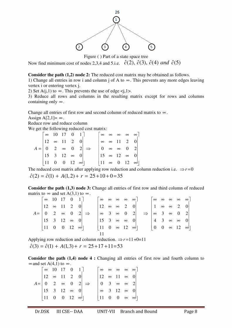
Dr.DSK III CSE-- DAA UNIT-VII Branch and Bound Page 8
Figure ( ) Part of a state space tree
Now find minimum cost of nodes 2,3,4 and 5.i.e. ˆ ˆ ˆ ˆ(2), (3), (4) (5)c c c and c
Consider the path (1,2) node 2: The reduced cost matrix may be obtained as follows.
1) Change all entries in row i and column j of A to ∞ . This prevents any more edges leaving
vertex i or entering vertex j.
2) Set A(j,1) to ∞ . This prevents the use of edge <j,1>.
3) Reduce all rows and columns in the resulting matrix except for rows and columns
containing only ∞ .
Change all entries of first row and second column of reduced matrix to ∞ .
Assign A[2,1]= ∞ .
Reduce row and reduce column
We get the following reduced cost matrix:
10 17 0 1
12 11 2 0
0 2 0 2
15 3 12 0
11 0 0 12
A
∞
∞ = ∞
∞
∞
⇒
11 2 0
0 0 2
15 12 0
11 0 12
∞ ∞ ∞ ∞ ∞ ∞ ∞ ∞ ∞
∞ ∞
∞ ∞
The reduced cost matrix after applying row reduction and column reduction i.e. 0r⇒ =
ˆ ˆ(2) (1) (1, 2) 25 10 0 35c c A r= + + = + + =
Consider the path (1,3) node 3: Change all entries of first row and third column of reduced
matrix to ∞ and set A(3,1) to ∞ .
10 17 0 1
12 11 2 0
0 2 0 2
15 3 12 0
11 0 0 12
A
∞
∞ = ∞
∞
∞
⇒
12 2 0
3 0 2
15 3 0
11 0 12
∞ ∞ ∞ ∞ ∞
∞ ∞ ∞ ∞
∞ ∞
∞ ∞
1 2 0
3 0 2
4 3 0
0 0 12
∞ ∞ ∞ ∞ ∞
∞ ∞ ⇒ ∞ ∞
∞ ∞
∞ ∞
11
Applying row reduction and column reduction. 11r⇒ = +0=11
ˆ ˆ(3) (1) (1,3) 25 17 11 53c c A r= + + = + + =
Consider the path (1,4) node 4 : Changing all entries of first row and fourth column to
∞ and set A(4,1) to ∞ .
10 17 0 1
12 11 2 0
0 2 0 2
15 3 12 0
11 0 0 12
A
∞
∞ = ∞
∞
∞
⇒
12 11 0
0 3 2
3 12 0
11 0 0
∞ ∞ ∞ ∞ ∞
∞ ∞ ∞ ∞
∞ ∞ ∞ ∞

Dr.DSK III CSE-- DAA UNIT-VII Branch and Bound Page 9
Applying row reduction and column reduction, 0r⇒ =
ˆ ˆ(4) (1) (1, 4) 25 0 0 25c c A r= + + = + + =
Consider the path (1,5) node 5: Changing all entries of first row and fifth column to ∞ and
set A(5,1) to ∞ . Reduce row and columns.
10 17 0 1
12 11 2 0
0 2 0 2
15 3 12 0
11 0 0 12
A
∞
∞ = ∞
∞
∞
⇒
12 11 2 2
0 3 0
15 3 12 3
0 0 12
∞ ∞ ∞ ∞ ∞
∞ ∞ ∞ ∞
∞ ∞
∞ ∞
10 9 0
0 3 0
12 0 9
0 0 12
∞ ∞ ∞ ∞ ∞
∞ ∞ ⇒ ∞ ∞
∞ ∞
∞ ∞
5
Applying row reduction and column reduction, 5r⇒ =
ˆ ˆ(5) (1) (1,5) 25 1 5 31c c A r= + + = + + =
ˆ ˆ ˆ ˆ(2) 35, (3) 53, (4) 25 (5) 31c c c and c= = = =
Since the minimum cost is 25, select node 4.
The matrix obtained for path (1,4) is considered as reduced cost matrix.
12 11 0
0 3 2
3 12 0
11 0 0
A
∞ ∞ ∞ ∞ ∞
∞ ∞ = ∞ ∞
∞ ∞ ∞ ∞
Now node 4 becomes E-node. Its children 6,7, and 8 are generated. The cost values are
calculated for nodes 6,7 and 8.
Figure ( ) Part of a state space tree
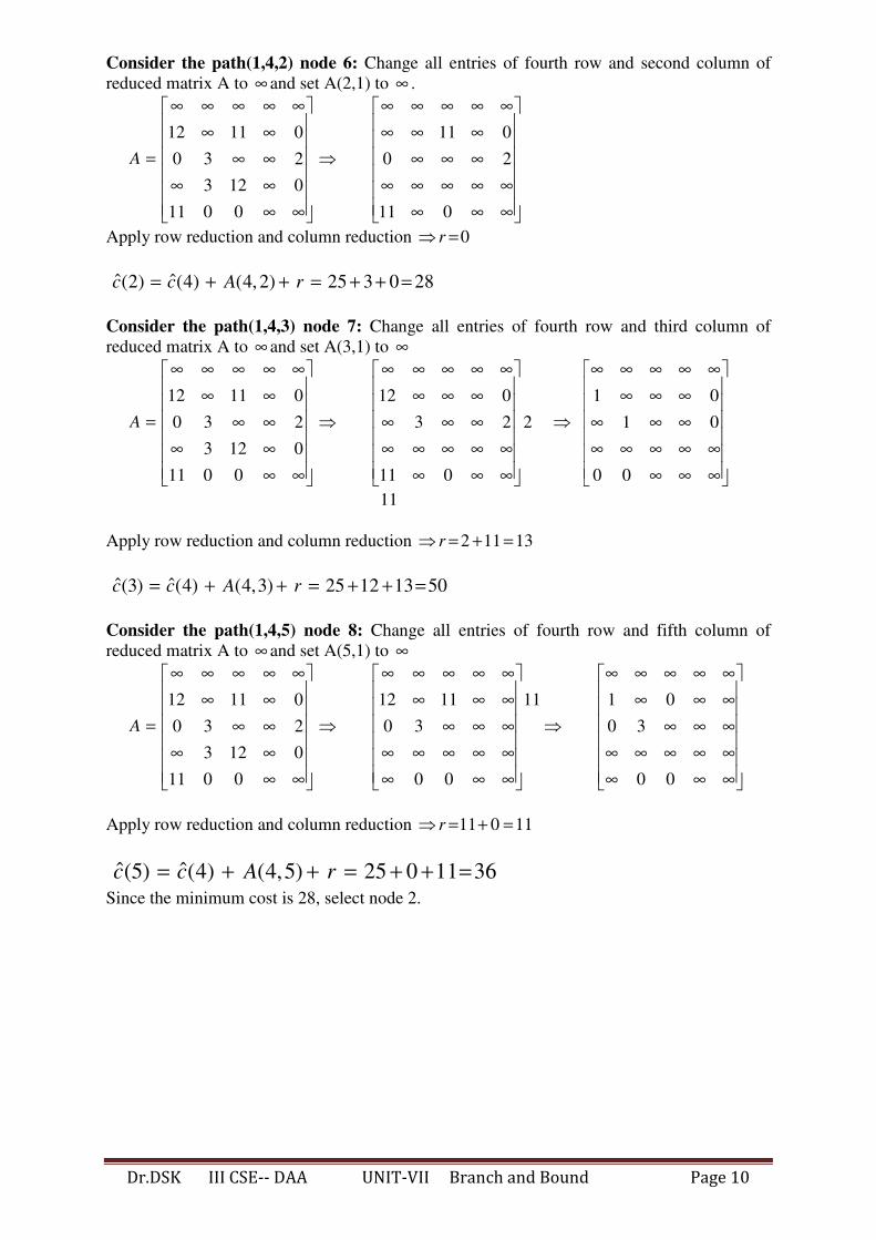
Dr.DSK III CSE-- DAA UNIT-VII Branch and Bound Page 10
Consider the path(1,4,2) node 6: Change all entries of fourth row and second column of
reduced matrix A to ∞ and set A(2,1) to ∞ .
12 11 0
0 3 2
3 12 0
11 0 0
A
∞ ∞ ∞ ∞ ∞
∞ ∞ = ∞ ∞
∞ ∞ ∞ ∞
⇒
11 0
0 2
11 0
∞ ∞ ∞ ∞ ∞ ∞ ∞ ∞ ∞ ∞ ∞
∞ ∞ ∞ ∞ ∞ ∞ ∞ ∞
Apply row reduction and column reduction 0r⇒ =
ˆ ˆ(2) (4) (4, 2) 25 3 0 28c c A r= + + = + + =
Consider the path(1,4,3) node 7: Change all entries of fourth row and third column of
reduced matrix A to ∞ and set A(3,1) to ∞
12 11 0
0 3 2
3 12 0
11 0 0
A
∞ ∞ ∞ ∞ ∞
∞ ∞ = ∞ ∞
∞ ∞ ∞ ∞
⇒
12 0
3 2 2
11 0
∞ ∞ ∞ ∞ ∞
∞ ∞ ∞ ∞ ∞ ∞
∞ ∞ ∞ ∞ ∞ ∞ ∞ ∞
1 0
1 0
0 0
∞ ∞ ∞ ∞ ∞
∞ ∞ ∞ ⇒ ∞ ∞ ∞
∞ ∞ ∞ ∞ ∞ ∞ ∞ ∞
11
Apply row reduction and column reduction 2 11 13r⇒ = + =
ˆ ˆ(3) (4) (4,3) 25 12 13 50c c A r= + + = + + =
Consider the path(1,4,5) node 8: Change all entries of fourth row and fifth column of
reduced matrix A to ∞ and set A(5,1) to ∞
12 11 0
0 3 2
3 12 0
11 0 0
A
∞ ∞ ∞ ∞ ∞
∞ ∞ = ∞ ∞
∞ ∞ ∞ ∞
⇒
12 11 11
0 3
0 0
∞ ∞ ∞ ∞ ∞
∞ ∞ ∞ ∞ ∞ ∞
∞ ∞ ∞ ∞ ∞ ∞ ∞ ∞
⇒
1 0
0 3
0 0
∞ ∞ ∞ ∞ ∞
∞ ∞ ∞ ∞ ∞ ∞
∞ ∞ ∞ ∞ ∞ ∞ ∞ ∞
Apply row reduction and column reduction 11 0 11r⇒ = + =
ˆ ˆ(5) (4) (4,5) 25 0 11 36c c A r= + + = + + =
Since the minimum cost is 28, select node 2.

Dr.DSK III CSE-- DAA UNIT-VII Branch and Bound Page 11
Figure ( ) Part of the state space tree
Consider the path(1,4,2,3) node 9: Change all entries of second row and third column to
∞ and set A(3,1) to ∞
11 0
0 2
11 0
A
∞ ∞ ∞ ∞ ∞ ∞ ∞ ∞ = ∞ ∞ ∞
∞ ∞ ∞ ∞ ∞ ∞ ∞ ∞
⇒ 2 2
11
∞ ∞ ∞ ∞ ∞ ∞ ∞ ∞ ∞ ∞ ∞ ∞ ∞ ∞
∞ ∞ ∞ ∞ ∞ ∞ ∞ ∞ ∞
⇒ 0
0
∞ ∞ ∞ ∞ ∞ ∞ ∞ ∞ ∞ ∞ ∞ ∞ ∞ ∞
∞ ∞ ∞ ∞ ∞ ∞ ∞ ∞ ∞
11
Apply row reduction and column reduction 2 11 13r⇒ = + =
ˆ ˆ(3) (2) (2,3) 28 11 13 52c c A r= + + = + + =
Consider the path (1,4,2,5) node 10: Change all entries of second row and fifth column to
∞ and set A(5,1) to ∞
11 0
0 2
11 0
A
∞ ∞ ∞ ∞ ∞ ∞ ∞ ∞ = ∞ ∞ ∞
∞ ∞ ∞ ∞ ∞ ∞ ∞ ∞
⇒ 0
0
∞ ∞ ∞ ∞ ∞ ∞ ∞ ∞ ∞ ∞ ∞ ∞ ∞ ∞
∞ ∞ ∞ ∞ ∞ ∞ ∞ ∞ ∞
Apply row reduction and column reduction 0r⇒ =
ˆ ˆ(3) (5) (5,3) 28 0 0 28c c A r= + + = + + =
Since minimum cost is 28, select node 5.
The matrix obtained for path (2,5) is considered as reduced cost matrix.

Dr.DSK III CSE-- DAA UNIT-VII Branch and Bound Page 12
Consider the path (1,4,2,5,3) node 11: Change all entries of fifth row and third column to
∞ and set A(3,1) to ∞
0
0
A
∞ ∞ ∞ ∞ ∞ ∞ ∞ ∞ ∞ ∞ = ∞ ∞ ∞ ∞
∞ ∞ ∞ ∞ ∞ ∞ ∞ ∞ ∞
⇒
∞ ∞ ∞ ∞ ∞ ∞ ∞ ∞ ∞ ∞ ∞ ∞ ∞ ∞ ∞
∞ ∞ ∞ ∞ ∞ ∞ ∞ ∞ ∞ ∞
Apply row reduction and column reduction 0r⇒ =
ˆ ˆ(3) (5) (5,3) 28 0 0 28c c A r= + + = + + =
Figure ( ) Final State Space Tree
The path is 1-4-2-5-3-1
Minimum cost=10+6+2+7+3=28
LCBB terminates with 1,4,2,5,3,1 as the shortest length tour.
Dr.DSK III CSE-- DAA UNIT-VII Branch and Bound Page 13
0/1 Knapsack problem::LCBB solution
The 0/1 knapsack problem states that, there are n objects given and capacity of knapsack is
m. Then select some objects to fill the knapsack in such a way that it should not exceed the
capacity of knapsack and maximum profit can be earned.
The 0/1 knapsack problem can be stated as
1 1 2 2 .....n n
Max z p x p x p x= + + +
1 1 2 2 .....n n
w x w x w x m+ + + ≤
Xi=0 or 1.
A branch and bound technique is used to find solution to the knapsack problem. But we
cannot directly apply the branch and bound technique to the knapsack problem. Because the
branch and bound deals with only minimization problems. We modify the knapsack problem
to the minimization problem. The modified problem is
1 1 2 2 .....n n
Min z p x p x p x= − − − −
1 1 2 2 .....n n
w x w x w x m+ + + ≤
Xi=0 or 1.
Let ˆ( )c x and ˆ( )u x are the two cost functions such that ˆ ˆ( ) ( ) ( )c x c x u x≤ ≤ satisfying the
requirements where 1
( )n
i i
i
c x p x=
= −∑ . The c(x) is the cost function for answer node x, which
lies between two functions called lower and upper bounds for the cost function c(x). The
search begins at the root node. Initially we compute the lower and upper bound at root node
called ˆ(1)c and ˆ(1)u . Consider the first variable x1 to take a decision. The x1 takes values
either 0 or 1. Compute the lower and upper bounds in each case of variable. These are the
nodes at the first level. Select the node whose cost is minimum i.e.
( ) min{ ( ( )), ( ( ))}c x c lchild x c rchild x=
ˆ ˆ( ) min{ (2)), (3))}c x c c=
The problem can be solved by making a sequence of decisions on the variables x1,x2,…,xn
level wise. A decision on the variable xi involves determining which of the values 0 or 1 is to
be assigned, to it by defining c(x) recursively.
The path from root to the leaf node whose height is maximum is selected and is the solution
space for the knapsack problem.
Dr.DSK III CSE-- DAA UNIT-VII Branch and Bound Page 14
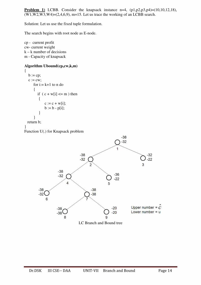
Problem 1) LCBB. Consider the knapsack instance n=4, (p1,p2,p3,p4)=(10,10,12,18),
(W1,W2,W3,W4)=(2,4,6,9), m=15. Let us trace the working of an LCBB search.
Solution: Let us use the fixed tuple formulation.
The search begins with root node as E-node.
cp - current profit
cw- current weight
k – k number of decisions
m - Capacity of knapsack
Algorithm Ubound(cp,cw,k,m)
{
b := cp;
c := cw;
for i:= k+1 to n do
{
if ( c + w[i] <= m ) then
{
c := c + w[i];
b := b - p[i];
}
}
return b;
}
Function U(.) for Knapsack problem
LC Branch and Bound tree
Dr.DSK III CSE-- DAA UNIT-VII Branch and Bound Page 15
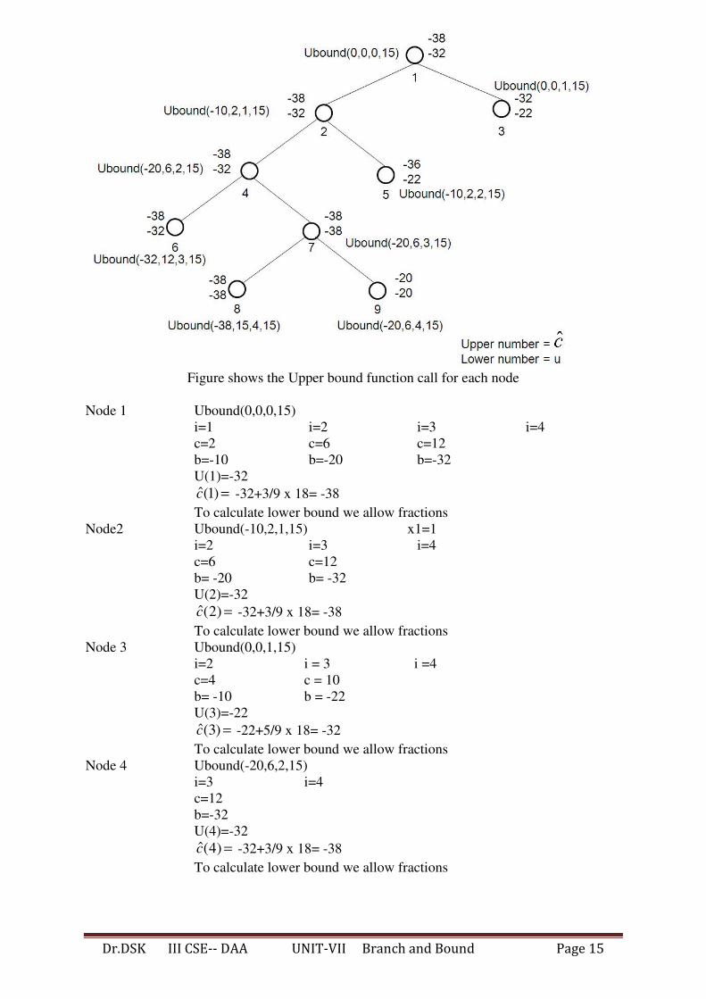
Figure shows the Upper bound function call for each node
Node 1 Ubound(0,0,0,15)
i=1
c=2
b=-10
i=2
c=6
b=-20
i=3
c=12
b=-32
i=4
U(1)=-32
ˆ(1)c = -32+3/9 x 18= -38
To calculate lower bound we allow fractions
Node2 Ubound(-10,2,1,15) x1=1
i=2
c=6
b= -20
i=3
c=12
b= -32
i=4
U(2)=-32
ˆ(2)c = -32+3/9 x 18= -38
To calculate lower bound we allow fractions
Node 3 Ubound(0,0,1,15)
i=2
c=4
b= -10
i = 3
c = 10
b = -22
i =4
U(3)=-22
ˆ(3)c = -22+5/9 x 18= -32
To calculate lower bound we allow fractions
Node 4 Ubound(-20,6,2,15)
i=3
c=12
b=-32
i=4
U(4)=-32
ˆ(4)c = -32+3/9 x 18= -38
To calculate lower bound we allow fractions

Dr.DSK III CSE-- DAA UNIT-VII Branch and Bound Page 16
Node 5 Ubound(-10,2,2,15)
i=3
c=8
b=-22
i=4
U(5)=-22
ˆ(5)c = -22+7/9 x 18= -36
To calculate lower bound we allow fractions
Node 6 Ubound(-32,12,3,15)
i=4
U(6)=-32
ˆ(6)c = -32+3/9 x 18= -38
To calculate lower bound we allow fractions
Node 7 Ubound(-20,6,3,15)
i=4
c=15
b=-38
U(7)=-38
ˆ(7)c = -38
Node 8 Ubound(-38,15,4,15)
U(8)=-38
ˆ(8)c = -38
Node 9 Ubound(-20,6,4,15)
U(1)=-20
ˆ(1)c = -20
Node 8 is a solution node (solution vector)
X1=1
X2=1
X3=0
X4=1
p1x1+p2x2+p3x3+p4x4
10x1+10=1+12x0+18x1
=38
We need to consider all n items.
The tuple size is n
Dr.DSK III CSE-- DAA UNIT-VII Branch and Bound Page 17
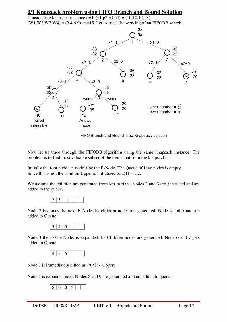
0/1 Knapsack problem using FIFO Branch and Bound Solution Consider the knapsack instance n=4, (p1,p2,p3,p4) = (10,10,12,18),
(W1,W2,W3,W4) = (2,4,6,9), m=15. Let us trace the working of an FIFOBB search.
Now let us trace through the FIFOBB algorithm using the same knapsack instance. The
problem is to find most valuable subset of the items that fit in the knapsack.
Initially the root node i.e. node 1 be the E-Node. The Queue of Live nodes is empty.
Since this is not the solution Upper is initialized to u(1) = -32.
We assume the children are generated from left to right. Nodes 2 and 3 are generated and are
added to the queue.
2 3
Node 2 becomes the next E Node. Its children nodes are generated. Node 4 and 5 and are
added to Queue.
3 4 5
Node 3 the next e-Node, is expanded. Its Children nodes are generated. Node 6 and 7 gets
added to Queue.
4 5 6
Node 7 is immediately killed as ˆ(7)c > Upper.
Node 4 is expanded next. Nodes 8 and 9 are generated and are added to queue.
5 6 8 9

Dr.DSK III CSE-- DAA UNIT-VII Branch and Bound Page 18
Then upper is updated to U(9)= -38.
Nodes 5 and 6 are the next two nodes to become E-Nodes. Neither is expanded as for each
ˆ()c > upper.
Node 8 is the next E-Node. Nodes 10 and 11 are generated.
9
Node 10 is infeasible and so killed.
Node 11 has ˆ()c > upper and so is also killed.
Node 9 is expanded Next. When node 12 is generated, upper and answer are updated to -38
and 12 respectively. Node 12 joins the queue of live nodes.
12
Node 13 is killed before it can get onto the queue of live nodes as ˆ(13)c > upper.
The only remaining live node is node 12. It has no children and the search terminates.
The value of upper and the path from node 12 to the root is the output additional information
is needed to determine the xi values on this path.
The solution is : x1=1, x2=1, x3=0,x4=1
Dr.DSK III CSE-- DAA UNIT-VII Branch and Bound Page 19
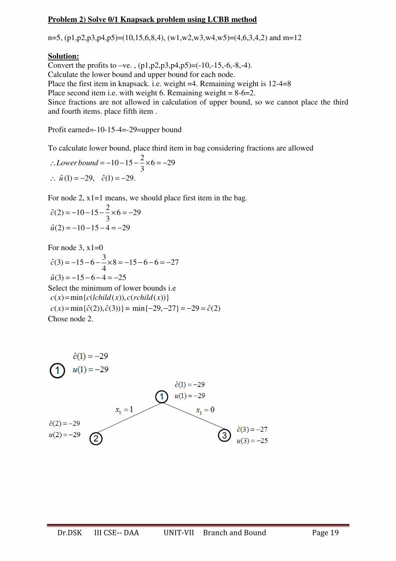
Problem 2) Solve 0/1 Knapsack problem using LCBB method
n=5, (p1,p2,p3,p4,p5)=(10,15,6,8,4), (w1,w2,w3,w4,w5)=(4,6,3,4,2) and m=12
Solution:
Convert the profits to –ve. , (p1,p2,p3,p4,p5)=(-10,-15,-6,-8,-4).
Calculate the lower bound and upper bound for each node.
Place the first item in knapsack. i.e. weight =4. Remaining weight is 12-4=8
Place second item i.e. with weight 6. Remaining weight = 8-6=2.
Since fractions are not allowed in calculation of upper bound, so we cannot place the third
and fourth items. place fifth item .
Profit earned=-10-15-4=-29=upper bound
To calculate lower bound, place third item in bag considering fractions are allowed
210 15 6 29
3Lower bound∴ = − − − × = −
ˆ ˆ(1) 29, (1) 29.u c∴ = − = −
For node 2, x1=1 means, we should place first item in the bag.
2ˆ(2) 10 15 6 29
3c = − − − × = −
ˆ(2) 10 15 4 29u = − − − = −
For node 3, x1=0
3ˆ(3) 15 6 8 15 6 6 27
4c = − − − × = − − − = −
ˆ(3) 15 6 4 25u = − − − = −
Select the minimum of lower bounds i.e
( ) min{ ( ( )), ( ( ))}c x c lchild x c rchild x=
ˆ ˆ( ) min{ (2)), (3))}c x c c= = ˆmin{ 29, 27} 29 (2)c− − = − =
Chose node 2.

Dr.DSK III CSE-- DAA UNIT-VII Branch and Bound Page 20

Dr.DSK III CSE-- DAA UNIT-VII Branch and Bound Page 21
LCBB Tree
The path is 1-2-4-7-9-10
The solution for knapsack problem is (x1,x2,x3,x4,x5)=(1,1,0,0,1)
Maximum profit = 10+15+4=29.
Dr.DSK III CSE-- DAA UNIT-VII Branch and Bound Page 22
Important Questions
1)Explain the general method of Branch and Bound.
2)Explain the properties of LC-search
3)Explain the method or reduction to solve TSP problem using Branch and Bound
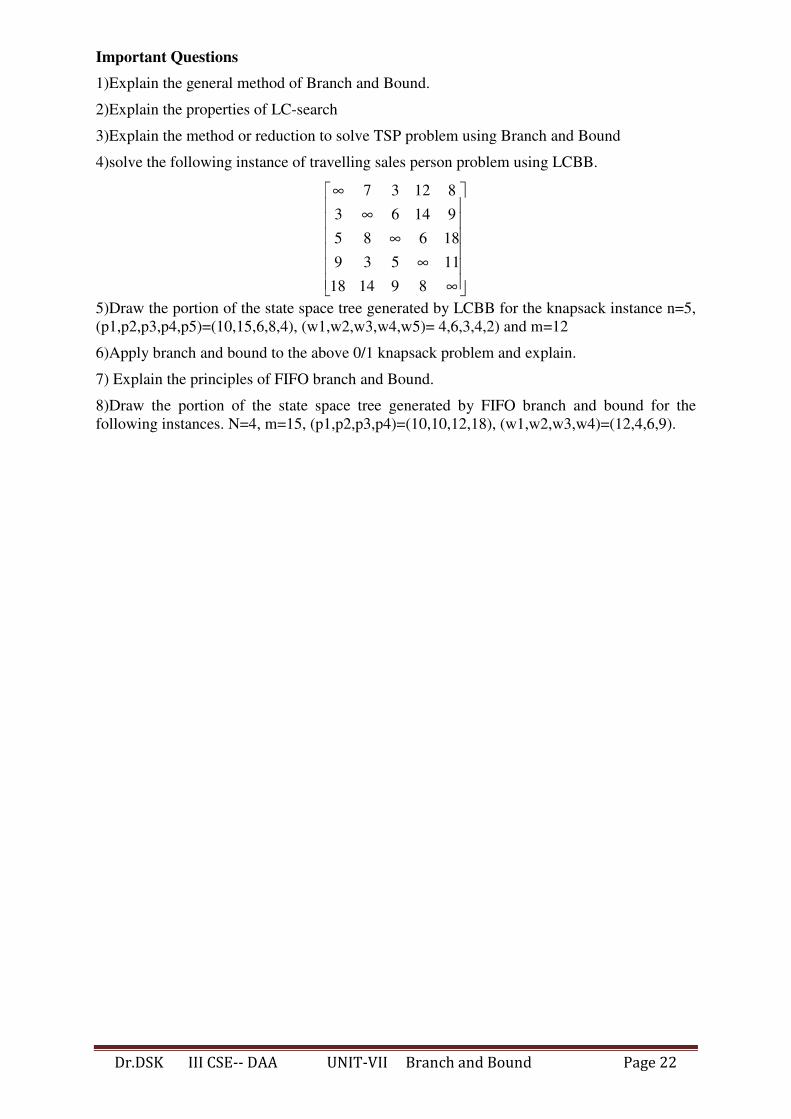
4)solve the following instance of travelling sales person problem using LCBB.
7 3 12 8
3 6 14 9
5 8 6 18
9 3 5 11
18 14 9 8
∞
∞ ∞
∞
∞
5)Draw the portion of the state space tree generated by LCBB for the knapsack instance n=5,
(p1,p2,p3,p4,p5)=(10,15,6,8,4), (w1,w2,w3,w4,w5)= 4,6,3,4,2) and m=12
6)Apply branch and bound to the above 0/1 knapsack problem and explain.
7) Explain the principles of FIFO branch and Bound.
8)Draw the portion of the state space tree generated by FIFO branch and bound for the
following instances. N=4, m=15, (p1,p2,p3,p4)=(10,10,12,18), (w1,w2,w3,w4)=(12,4,6,9).
![DAA MID2 [UandiStar.org]](https://static.fdocuments.us/doc/165x107/545a7372af7959755d8b5b4b/daa-mid2-uandistarorg.jpg)


