Grant Agreement number: 313243 Project acronym: SUNNY Project title: Smart UNattended airborne sensor Network for detection of vessels used for cross border crime and irregular entrY Funding Scheme: Collaborative project

D3.1: Thermal/infrared sensing - FV

Due date of deliverable: 29/02/2016 Actual submission date: 15/06/2016 Start date of project: 01/01/2014 Duration: 42 Months Organisation name of lead contractor for this deliverable: Xenics (XEN) Participating: XEN, TEC

Project co-funded by the European Commission within the Seventh Framework Programme (2007-2013) Dissemination Level PU Public PP Restricted to other programme participants (including the Commission Services) RE Restricted to a group specified by the consortium (including the Commission

CO Confidential, only for members of the consortium (including the Commission Services)

Document Title: WP Document number:

Thermal/infrared sensing WP3 T3.1 D3.1

Main Authors Org

Das Jo XEN

Contributing Authors Org

José Ramón Garcia Martinez TEC

Doc. History Version Comments Date Authorised by

1 V1 Version 1, ready for internal review 31/12/15 2 V2 Version 2, ready for internal review 14/06/16 Number of pages: 35 Number of annexes:

Contents CONTENTS ........................................................................................................................................................ 3

0. REVISION HISTORY ...................................................................................................................................................... 4 1. EXECUTIVE SUMMARY ................................................................................................................................................. 7 2. INTRODUCTION .......................................................................................................................................................... 9

2.1 SUNNY Project Objectives ............................................................................................................................. 9 2.2 This Version ................................................................................................................................................... 9 2.3 Document Conventions & Glossary ............................................................................................................. 10

3. SWIR SENSOR SPECIFICATION, PERFORMANCE AND QUALIFICATION TESTS ........................................................................... 11 3.1 Introduction ................................................................................................................................................ 11 3.2 SWIR Sensor design overview ..................................................................................................................... 11 3.3 SWIR sensor specifications .......................................................................................................................... 12 3.4 XSW functionality, performance and qualification tests ............................................................................. 15 3.5 XSW field tests: first results ......................................................................................................................... 23 3.6 XSW summary and conclusions ................................................................................................................... 24

4. LWIR SENSOR SPECIFICATION, PERFORMANCE AND QUALIFICATION TESTS ............................................................................ 25 4.1 Introduction ................................................................................................................................................ 25 4.2 LWIR Sensor design overview ...................................................................................................................... 25 4.3 LWIR sensor specifications .......................................................................................................................... 26 4.4 XTM functionality, performance and qualification tests ............................................................................. 29 4.1 XTM field tests: first results ......................................................................................................................... 32 4.2 XTM summary and conclusions ................................................................................................................... 34

5. GENERAL CONCLUSIONS ............................................................................................................................................ 35 6. REFERENCES ............................................................................................................................................................ 35

0. Revision History

Revision Date Section Changes Changed by

V1 31/12/2015 First version for internal review J. Das V2 15/06/2016 2nd version for internal review J. Das

Table 0-1 Revision history

List of Figures FIGURE 3-1 FUNCTIONAL DIAGRAM OF XSW CORE ...................................................................................................................... 11 FIGURE 3-2 MECHANICAL DRAWING OF THE XSW (WITHOUT LENS) ................................................................................................ 14 FIGURE 3-3 MECHANICAL DRAWING OF THE XSW (WITH LENS) ...................................................................................................... 14 FIGURE 3-4 RESIDUAL NON-UNIFORMITY AFTER TRUENUC CORRECTION .......................................................................................... 16 FIGURE 3-5 ILLUSTRATION OF THE AUTO-EXPOSURE ALGORITHM ..................................................................................................... 16 FIGURE 3-6 COMPARISON OF VISUAL IMAGE [A], SWIR IMAGE WITH TRUENUC [B], TRUENUC + AGC [C], TRUENUC + AGC + HE [D] .. 17 FIGURE 3-7 QUANTUM EFFICIENCY MEASUREMENT ...................................................................................................................... 18 FIGURE 3-8 FPA TEMPERATURE AS A FUNCTION OF THE TEC POWER DUTY CYCLE AND THE CLIMATE CHAMBER TEMPERATURE .................... 19 FIGURE 3-9 CAMERA POWER CONSUMPTION AS A FUNCTION OF TEC POWER PERCENTAGE AND CLIMATE CHAMBER TEMPERATURE ............. 19 FIGURE 3-10 DARK SIGNAL MEASUREMENTS LOW GAIN (LEFT) AND HIGH GAIN (RIGHT) ..................................................................... 20 FIGURE 3-11 DARK CURRENT AS FUNCTION OF BIAS AND TEMPERATURE ........................................................................................... 21 FIGURE 3-12 DARK CURRENT AS DISTRIBUTION OVER THE WAFER .................................................................................................... 21 FIGURE 3-13 TEMPORAL NOISE IN HIGH GAIN (LEFT) AND LOW GAIN (RIGHT), MEASURED IN DARK AT 100US INTEGRATION TIME. ............... 21 FIGURE 3-14 BAD PIXEL MAP XSW ........................................................................................................................................... 22 FIGURE 3-15 COMPARISON SWIR AND VISUAL SENSOR ................................................................................................................ 23 FIGURE 3-16 FIELD TEST AT BELGIAN COAST ............................................................................................................................... 23 FIGURE 4-1 FUNCTIONAL DIAGRAM OF XTM CORE ...................................................................................................................... 25 FIGURE 4-2 MECHANICAL DRAWING OF THE XTM (WITHOUT LENS) ................................................................................................ 28 FIGURE 4-3 MECHANICAL DRAWING OF THE XTM (WITH LENS) ...................................................................................................... 28 FIGURE 4-4 COMPARISON OF A LWIR IMAGE BEFORE (LEFT) AND AFTER (RIGHT) AGC: THE AGC ALGORITHM STRETCHES THE HISTOGRAM TO

IMPROVE THE CONTRAST IN THE IMAGE. ............................................................................................................................ 29 FIGURE 4-5 COMPARISON OF A LWIR IMAGE BEFORE (LEFT) AND AFTER (RIGHT) XIE: THE XIE ALGORITHM CLEARLY SHARPENS THE OBJECTS IN

THE IMAGE. ................................................................................................................................................................. 30 FIGURE 4-6 COMPARISON OF A LWIR IMAGE BEFORE (LEFT) AND AFTER (RIGHT) HISTOGRAM EQUALIZATION. ........................................ 30 FIGURE 4-7 PERCENTILE AVERAGE ADU VALUES OF ULIS 55MK ..................................................................................................... 31 FIGURE 4-8 BAD PIXEL MAP OF THE XTM ................................................................................................................................... 32 FIGURE 4-9 COMPARISON VISUAL (LEFT) AND LWIR IMAGE (RIGHT) IN A MARITIME SCENARIO ............................................................. 33 FIGURE 4-10 FIELD TEST RESULT, DONE BY INESC / CINAV ............................................................................................................. 33

List of Tables TABLE 0-1 REVISION HISTORY .................................................................................................................................................... 4 TABLE 2-1 GLOSSARY TABLE .................................................................................................................................................... 10 TABLE 3-1 XSW DETECTOR SPECIFICATIONS ............................................................................................................................... 12 TABLE 3-2 XSW SENSOR SPECIFICATIONS .................................................................................................................................. 12 TABLE 3-3 XSW OPTICAL LENS SPECIFICATIONS ........................................................................................................................... 13 TABLE 3-4 XSW VIDEO DATA OUTPUT SPECIFICATION ................................................................................................................... 13 TABLE 3-5 XSW POWER CONSUMPTION SPECIFICATION................................................................................................................ 13 TABLE 3-6 XSW SENSOR CONTROL SPECIFICATION ...................................................................................................................... 13 TABLE 3-7 XSW MECHANICAL SPECIFICATIONS ........................................................................................................................... 14 TABLE 3-8 XSW ENVIRONMENTAL SPECIFICATIONS ...................................................................................................................... 15 TABLE 3-9 XSW TEST RESULTS................................................................................................................................................. 24 TABLE 4-1 XTM DETECTOR SPECIFICATIONS ............................................................................................................................... 26 TABLE 4-2 XTM SENSOR SPECIFICATIONS .................................................................................................................................. 26 TABLE 4-3 OPTICAL LENS SPECIFICATIONS ................................................................................................................................... 27 TABLE 4-4 LWIR GASIR FL25MM LENS SPECIFICATIONS............................................................................................................... 27 TABLE 4-5 XTM VIDEO DATA OUTPUT SPECIFICATION ................................................................................................................... 27 TABLE 4-6 XTM POWER CONSUMPTION SPECIFICATION ................................................................................................................ 27 TABLE 4-7 XTM SENSOR CONTROL SPECIFICATION ...................................................................................................................... 27 TABLE 4-8 XTM MECHANICAL SPECIFICATIONS ........................................................................................................................... 28 TABLE 4-9 XTM ENVIRONMENTAL SPECIFICATIONS ...................................................................................................................... 28 TABLE 4-10 XTM TEST RESULTS ............................................................................................................................................... 34

1. Executive Summary

The SUNNY project aims to develop and integrate a new tool for collecting real-time information using heterogeneous sensors carried by multiple UAV platforms, and for analyzing this information automatically to provide situational awareness for the system operators to monitor the EU maritime borders more effectively and efficiently. In this document, we will describe the specification, performance and qualification tests of the infrared sensors. Two infrared sensors are developed by Xenics: a SWIR sensor (XSW) and a LWIR sensor (XTM). The XSW will be integrated on the Etheras UAV: the sensor will be put into an OTUS-U135 gimbal from DST. The XSW comprises the following building blocks:

- Optical interface (25mm SWIR lens) - SWIR InGaAs based detector (640 x 512), with TE1 temperature stabilization - Sensor front end electronics (sensor biasing, ADC electronics and TEC control) - FPGA platform: The FPGA controls the detector sequencing and processes the incoming detector

data. The following algorithms are developed for the XSW: o NUC (non-uniformity correction) o Auto-exposure o Auto-gain o Histogram equalization

- Power, Serial control and Video-interface (PAL) The following tests have been executed on the XSW:

- Functionality tests o Exposure time range o On-board algorithms o Serial control

- Performance tests o Spectral response (0.9 – 1.7 µm) o Power consumption

- Environmental tests o Storage and operational temperature range

- Qualification tests o Dark current, noise and bad pixel analysis

Finally, the performance of the XSW was tested in the field in different conditions, in order to do an initial comparison with a visual sensor.

The second developed infrared sensor is the XTM. The XTM will be integrated on the SCRAB-II UAV. The sensor will be put together with an E/O sensor (FCB-H11 from Sony) into an OTUS L170 gimbal from DST. The XTM comprises the following building blocks:

- Optical interface: (25mm LWIR lens) - Bolometer detector (640 x 480) - Shutter, and shutter drive electronics for offset correction - Front end electronics (sensor biasing and ADC) - FPGA platform: The FPGA controls the detector sequencing and processes the incoming detector

data. The following algorithms are developed for the XTM: o NUC (non-uniformity correction) o Auto-gain o Histogram equalization o XIE (Xenics image enhancement)

- Power, Serial control and video interface (PAL). The following tests have been executed on the XTM:

- Functionality tests o Exposure time range o On-board algorithms o Serial control

- Performance tests o NETD o Power consumption

- Environmental tests o Storage and operational temperature range

- Qualification tests o Bad pixel analysis

Finally, the performance of the XTM was tested in the field in order to test the sensor in a maritime scenario and to do an initial comparison with a visual sensor.

2. Introduction

2.1 SUNNY Project Objectives

The SUNNY project aims to contribute to EUROSUR by defining a new tool for collecting real-time information in operational scenarios. SUNNY represents a step beyond existing research projects due to the following main features:

A two-tier intelligent heterogeneous Unmanned Aerial Vehicle (UAV) sensor network will be

considered in order to provide both large field and focused surveillance capabilities, where the first-tier sensors, carried by medium altitude, long-endurance autonomous UAVs, are used to patrol large border areas to detect suspicious targets and provide global situation awareness. Fed with the information collected by the first-tier sensors, the second-tier sensors will be deployed to provide more focused surveillance capability by tracking the targets and collecting further evidence for more accurate target recognition and threat evaluation. Novel algorithms will be developed to analyse the data collected by the sensors for robust and accurate target identification and event detection;

Novel sensors and on-board processing generation, integrated on UAV system, will be focus on

low weight, low cost, high resolution that can operate under variable conditions such as darkness, snow, and rain. In particular, SUNNY will develop sensors that generate both RGB image, Near Infrared (NIR) image and hyperspectral image and that use radar information to detect, discriminate and track objects of interest inside complex environment, with focus on the sea borders. Alloying to couple sensor processing and preliminary detection results (on-board) with local UAV control, leading to innovative active sensing techniques, replacing low-level sensor data communication by a higher abstraction level of information communication (Sunny, 2013).

2.2 This Version

This document is the final version of this deliverable.

2.3 Document Conventions & Glossary

Term Definition ADC Analog to digital conversion ADU Analog-to-digital unit AGC Auto Gain Control E/O Electro-optical FPA Focal Plane Array FTIR Fourrier Transform Infrared Spectroscopy LWIR Long Wave InfraRed NETD Noise Equivalent Temperature Difference NTC resistor Resistor with negative temperature coefficient, used for temperature

measurements NUC Non-uniformity correction SWIR Short Wave InfraRed TEC Thermo-electric cooler TE1 1-stage thermo-electric cooler UAV Unmanned Aerial Vehicle XIE Xenics Image Enhancement XSW Xenics’ ShortWave module sensor XTM Xenics’ Thermal Module sensor

Table 2-1 Glossary table

3. SWIR sensor specification, performance and qualification tests

3.1 Introduction

In this chapter we describe the functionality of the XSW-sensor, which is sensitive in the short-wave infrared (SWIR). We first give an overview of sensor design and a summary of the specifications. Afterwards, we discuss the different tests that were done in order to verify the requirements of the sensor.

3.2 SWIR Sensor design overview

Figure 3-1 Functional diagram of XSW core

Figure 3-1 shows the functional diagram of the XSW: a 640x512 InGaAs based detector is used for SWIR imaging. This detector is cooled using a TE1 thermoelectric cooler. The ROIC of the detector is based on a CTIA which can be used in high gain and low gain mode. Furthermore the ROIC can be used in ITR (integrate then read) or IWR (integrate while read) mode. The output of the detector is (after ADC conversion) is further processed in the FPGA of the XSW core. In a first step is the pixel correction to correct the fixed-pattern non-uniformity, photon-response non-uniformity and to replace bad pixels. In the second step, the resulting image is enhanced using the following algorithms:

Auto exposure: this algorithm is used to find the optimal exposure time Auto gain and offset: this algorithm stretches and/or shifts the image histogram Histogram Equalization: this algorithm is used to enhance the contrast in the

image These algorithms are configurable by the user using the serial control interface: different parameters can be modified in order to obtain the most optimal performance. In default mode, all algorithms will be enabled. In a final step the image is transmitted to the output PAL interface.

3.3 SWIR sensor specifications

3.3.1 XSW detector and general functionality specifications

An overview of the XSW detector and sensor functionality specifications are given in Table 3-1 and Table 3-2.

S2.1 Parameter Specification Unit Verification method

D = Design ; T=Test ; A =Analysis or Demo

S 2.1.01 Detector type InGaAs FPA; ROIC with CTIA topology (D)

S 2.1.02 Spectral Response 0.9-1.7 µm (T) S 2.1.03 Number of pixels 640x512 (D) S 2.1.04 Pixel pitch 20 µm (D) S 2.1.05 Dark Current 0.8 x106 electrons/s (T) S 2.1.06 Integration Capacitor

High Gain 2 fF (D)

S 2.1.07 Integration Capacitor Low Gain 85 fF (D)

S 2.1.08 Pixel operability > 99 % (T) S 2.1.09 Cooling TE1 (D)

Table 3-1 XSW Detector Specifications

S2.2 Parameter Specification Verification method D = Design ; T=Test ; A =Analysis or Demo

S 2.2.01 Frame rate 25Hz (D) S 2.2.02 Exposure time range 1-40000 µs (A) S 2.2.03 Gain (in High Gain mode) 1.28 electron/ADU (D)

Gain (in Low Gain mode) 16.2 electron/ADU (D) S 2.2.04 Core Read Noise Low Gain 400 electrons rms (T)

Core Read Noise High Gain 120 electrons rms (T)

S 2.2.05 Readout mode Integrate Then Read (ITR) Integrate While Read (IWR)

(D)

S 2.2.06

On-board image processing

o Imaging correction (fixed NUC for XSW-GigE, TrueNUC for all others),

o Auto-Gain and Offset o Auto-Exposure (except for

XSW-GigE) o Histogram Equalization o Trigger possibilities

(A)

Table 3-2 XSW Sensor Specifications

3.3.2 XSW optical specifications

The optical lens parameters are specified in Table 3-3. From these specifications, it was decided to use the SWIRECON 25mm lens together with the XSW. The specifications of this lens are summarized in Table 3-4.

S 2.6 Spectral Band Specifications Verification method

D = Design ; T=Test ; A =Analysis or Demo

S 2.6.01 SWIR (0.9-1.7µm) o Focal length: 25 mm o F-number: 1.8

(D)

Table 3-3 XSW Optical lens specifications

Parameter Specification Manufacturer OpticoElectron Product Number SWIRECON 25 Focal Length 25.0 mm Aperature-based f-number f/1.80 Waveband 0.6 – 1.7 µm Assembly Weight 92.5g Dimensions Diameter 32mm; length 49mm

Table 3-4 SWIR SWIRECON 25mm Lens Specifications

3.3.3 XSW Electrical Interface Specifications The electrical interface specifications of the XSW are summarized in Table 3-5, Table 3-6 and Table 3-7. A picture of the electrical interface is shown in Figure 3-2.

S 2.7 Sensor / Gimbal Video Data output specification Verification method

D = Design ; T=Test ; A =Analysis or Demo

S 2.7.01 XSW-640 SWIR PAL Connector: BNC

(D)

Table 3-5 XSW Video data output specification

S 2.8 Sensor / Gimbal Power Supply Power Consumption Verification method D = Design ; T=Test ; A =Analysis or Demo

S 2.8.01 XSW-640 (SWIR) 12 V ± 10% Connector: Hirose HR10-7R-4SA(73)

3(*) - 10(**) (*) without TEC (**) TEC at 100%

(T)

Table 3-6 XSW Power consumption specification

S 2.9 Sensor / Gimbal Sensor Control Specifications Verification method D = Design ; T=Test ; A =Analysis or Demo

S 2.9.01 XSW-640 (SWIR) serial control RS-232 Connector: RJ-12

(A)

Table 3-7 XSW Sensor Control specification

3.3.4 XSW Mechanical Specifications The mechanical specifications of the XSW are summarized in Table 3-9. The mechanical drawing is shown in Figure 3-2.

S 2.10 Mechanical size/weight

Specification Verification method D = Design ; T=Test ; A =Analysis or Demo

S 2.10.01 XSW size 45x45x68.1 mm3 (XSW-640-PAL) (D) SWIR lens size 25 mm lens: ≤50 mm(length) / ≤42 mm

(diameter) (D)

Total size SWIR 45x45x110 mm3 (D) S 2.10.02 XSW weight ≤150 g (XSW-640-PAL) (D)

SWIR lens weight 25 mm lens: ≤100 g (D) Total weight SWIR ≤300 g (XSW + optical front + lens) (D)

Table 3-8 XSW Mechanical specifications

Figure 3-2 Mechanical drawing of the XSW (without lens)

Figure 3-3 Mechanical drawing of the XSW (with lens)

3.3.5 XSW Environmental Specifications

The environmental specifications of the XSW are summarized in Table 3-9.

S 2.11 Environmental Parameter Specification Verification method S 2.11.01 XSW Operating case temperature -40 to 70°C (T) S 2.11.02 XSW Storage temperature -45 to 85°C (T)

Table 3-9 XSW Environmental specifications

3.4 XSW functionality, performance and qualification tests

3.4.1 Functionality tests

The following functionality tests are performed on the XSW, in order to verify the specifications: o Exposure time range

The exposure time range was tested: The camera allows an exposure range of 1µs to 40ms Using the auto-exposure the exposure time is be varied between:

o 100µs – 20ms (Low Gain) o 100µs – 20ms (High Gain – ITR) o 10ms – 40ms (High Gain – IWR)

o On-board algorithms TrueNUC control

To verify the TrueNUC control the The Residual Non-Uniformity is measured for the different TrueNUCs, over the complete integration range. Here the RNU is defined as:

The RNU is first measured at fixed 25 °C detector temperature, with a uniform illumination at 50% well fill. From the data we can derive that the RNU (compared to the average signal) stays <1% over the complete integration range.

Figure 3-4 Residual non-uniformity after TrueNUC correction

Auto exposure

The auto exposure algorithm on the XSW is changing the integration time, so that the image is not over- or underexposed. As there are different sensor gains (low gain) and read-out modes (ITR and IWR), the algorithm is implemented in such a way that it can also automatically switch between these different gains and modes. The algorithm is illustrated in Figure 3-5: due to changing conditions due to varying clouds, and night falling (the images are taken between 5 and 7pm), the gain mode and integration time are automatically adjusted to avoid saturation effects, and to maintain the overall brightness.

Figure 3-5 Illustration of the auto-exposure algorithm

Auto Gain (AGC) A second image enhancement algorithm is the auto-gain control (AGC) algorithm. This algorithm controls the offset and gain of the image manually or automatically. In automatic mode, the optimal gain and offset values are calculated to stretch the image as much as possible without introducing clipping. An example of an image before and after automatic AGC is shown in Figure 3-6 [B] and [C].

Histogram Equalization (HE) A final algorithm that is implemented on the XSW is histogram equalization. The histogram equalization algorithm uses the information of the accumulative histogram of the image to improve the contrast of the image. This is done by making the histogram distribution (more) uniform. The histogram equalization algorithm only changes the distribution of the histogram. The algorithm is very useful,

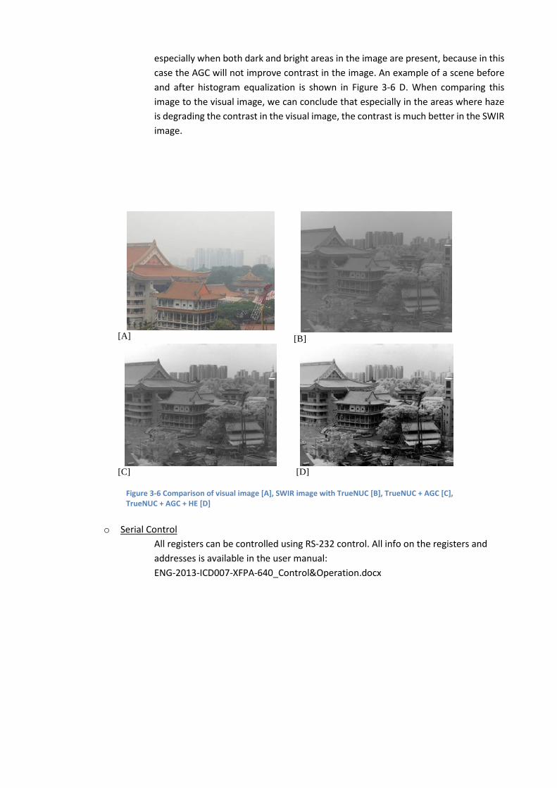
especially when both dark and bright areas in the image are present, because in this case the AGC will not improve contrast in the image. An example of a scene before and after histogram equalization is shown in Figure 3-6 D. When comparing this image to the visual image, we can conclude that especially in the areas where haze is degrading the contrast in the visual image, the contrast is much better in the SWIR image.

[A]

[B]

[C]

[D]

Figure 3-6 Comparison of visual image [A], SWIR image with TrueNUC [B], TrueNUC + AGC [C], TrueNUC + AGC + HE [D]

o Serial Control

All registers can be controlled using RS-232 control. All info on the registers and addresses is available in the user manual: ENG-2013-ICD007-XFPA-640_Control&Operation.docx

3.4.2 Performance tests

The following performance tests are performed on the XSW, in order to verify the specifications: o Spectral Response

The quantum efficiency of a 640x512 detector was measured using a FTIR setup. The result is shown in Figure 3-7.

Figure 3-7 Quantum efficiency measurement

o Power Consumption The power consumption is measured at different climate temperatures, and for different TEC duty cycle settings. With changing TEC duty cycle, the detector will be cooled more, but this will also increase the overall power consumption of the sensor. The detector FPA (focal plane array) temperature is measured with a NTC resistor which is located inside the detector package. In Figure 3-8, the FPA temperature is shown as function of the TEC duty cycle, at different climate chamber temperatures. The sensor can work up to 70°C, however at temperatures above 40°C, the TEC power has to be limited in order to prevent overheating (when overheating occurs, the module will shut down from itself). Figure 3-9 shows the power consumption of the sensor. At a TEC duty cycle of 100% the power consumption goes up to 10W.

Figure 3-8 FPA temperature as a function of the TEC power duty cycle and the climate chamber temperature

Figure 3-9 Camera power consumption as a function of TEC power percentage and climate chamber temperature

o Environmental tests The following environmental tests have been performed on the XSW:

Operating temperature range verification: -40 to 70°C The XSW was tested in the climate chamber for complete operating temperature range. At different temperatures, the following parameters were tested:

- Correct start-up after power down - Power consumption - Dark Current - Image quality (from RNU measurement)

The camera keeps functional over the specified temperature range.

Storage temperature range verification: -45 to 85°C After storage test at -45 and 85°C, the camera was tested to verify that there was no degradation. The following parameters were tested:

- Correct start-up after power down - Power consumption - Dark Current - Image quality (from RNU measurement)

No degradation was observed after the storage tests.

3.4.3 Qualification tests

On the XSW that will be used for the SUNNY demonstration, the following qualification tests are performed on the XSW, in order to verify the specifications: dark current, noise and bad pixel analysis. o Dark Current

The dark current is evaluated at different sensor temperatures (see Figure 3-10). The dark signal is given by:

𝜇𝜇𝑑𝑑 = 𝜇𝜇𝑑𝑑,0 + 𝜇𝜇𝐼𝐼 . 𝑡𝑡𝑒𝑒𝑒𝑒𝑒𝑒

In this equation, texp is the exposure time and µI is the dark current, expressed in electrons/s. Note that the gain values, to convert ADU to electrons is given by S2.2.03. From the dark signal measurements the dark current was extracted. The dark current as function of temperature, and at different bias voltages is shown in Figure 3-11. At 288K, and 250mV a dark current of 0.56x106 e/s was obtained.

O Figure 3-10 Dark signal measurements Low Gain (left) and High Gain (right)

Figure 3-11 Dark current as function of bias and temperature

Figure 3-12 Dark current as distribution over the wafer

o Noise The temporal noise of the detector was measured in dark at an integration time of 100µs. The noise pixel maps, measured in high and low gain are shown in Figure 3-13. The average value at high gain and low gain is 116 and 385 electrons respectively.

Figure 3-13 Temporal noise in high gain (left) and low gain (right), measured in dark at 100us integration

time.

o Bad Pixel Analysis

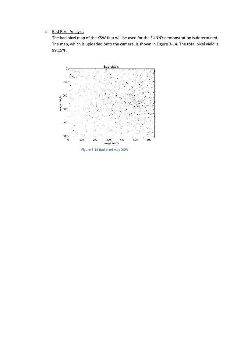
The bad pixel map of the XSW that will be used for the SUNNY demonstration is determined. The map, which is uploaded onto the camera, is shown in Figure 3-14. The total pixel yield is 99.15%.

Figure 3-14 Bad pixel map XSW

3.5 XSW field tests: first results

An XSW was tested in Leuven at the Xenics office and at the Belgian coast. The camera was compared with a commercial visual camera. The field test in Leuven was carried out during daytime, with fog conditions (see Figure 3-15). The tower, which is located at 4 km distance is almost not visible with the visual camera, but can clearly be detected with the SWIR camera. The second test was carried out along the Belgian coast, under good atmospheric conditions. An example is shown in Figure 3-16.

Further field test results will be reported in other deliverables.

Figure 3-15 Comparison SWIR and visual sensor

Figure 3-16 Field test at Belgian coast

3.6 XSW summary and conclusions

In this section, we have first discussed the architecture and specifications of the XSW SWIR sensor. The following tests were carried out in order to verify the requirements: - Functional tests - Performance tests - Environmental tests - Qualification tests - First field tests

An overview of the XSW test results is given in Table 3-10.

S Parameter Specification Measurement Result S 2.1.02 Spectral

Response 0.9-1.7µm 0.9-1.7 µm Ok

S 2.1.05 Dark Current 0.8 x106 electrons/s Ok S 2.1.08 Pixel operability > 99 % 99.15 % Ok S 2.2.02 Exposure time

range 1-40000 µs Ok

S 2.2.04 Core Read Noise Low Gain 400 electrons 385 electrons Ok

Core Read Noise High Gain 120 electrons 116 electrons Ok

S 2.2.06

On-board image processing

Imaging correction Auto-Gain and Offset Auto-Exposure Histogram Equalization Trigger possibilities

Ok

S 2.8.01 Power consumption

3(*) - 10(**) (*) without TEC (**) TEC at 100%

3-10 W Ok

S 2.9.01 XSW-640 (SWIR) serial control RS-232 Connector: RJ-12

Ok

S 2.11.01 XSW Operating case temperature

-40 to 70°C Ok

S 2.11.02 XSW Storage temperature -45 to 85°C Ok

Table 3-10 XSW Test results

4. LWIR sensor specification, performance and qualification tests

4.1 Introduction In this chapter we describe the functionality of the XTM-sensor (LWIR) which is sensitive in the longwave (thermal) infrared (LWIR). We first give an overview of sensor design and a summary of the specifications. Afterwards, we discuss the different tests that were done in order to verify the requirements of the sensor.

4.2 LWIR Sensor design overview

Figure 4-1 Functional diagram of XTM core

Figure 4-1 shows the functional diagram of the XTM core. A 640*480 bolometer detector with 17 µm pitch from ULIS is used in the XTM. After ADC conversion the image data is further processed in the FPGA of the XTM. In a first step is the pixel correction to correct the fixed-pattern non-uniformity, photon-response non-uniformity and to replace bad pixels. In the second step, the resulting image is enhanced using the following algorithms:

Auto gain and offset: this algorithm stretches and/or shifts the image histogram. XIE: a filter is applied in order to smooth or sharpen the image. Histogram Equalization: this algorithm is used to enhance the contrast in the

image. These algorithms are configurable by the user, using the serial control interface of the module. Different parameters can be modified in order to obtain the most optimal performance. In the default mode all algorithms are enabled.

4.3 LWIR sensor specifications

4.3.1 XTM detector and general functionality specifications

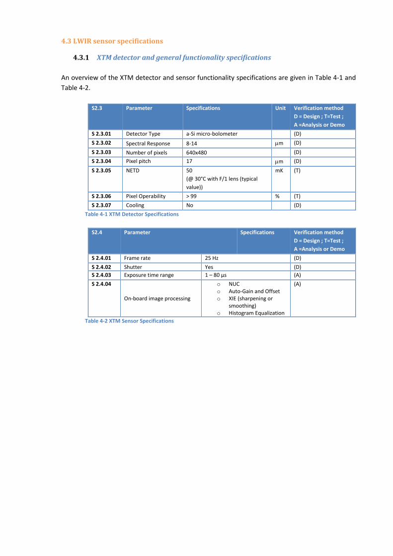
An overview of the XTM detector and sensor functionality specifications are given in Table 4-1 and Table 4-2.

S2.3 Parameter Specifications Unit Verification method

D = Design ; T=Test ; A =Analysis or Demo

S 2.3.01 Detector Type a-Si micro-bolometer (D) S 2.3.02 Spectral Response 8-14 µm (D) S 2.3.03 Number of pixels 640x480 (D) S 2.3.04 Pixel pitch 17 µm (D) S 2.3.05 NETD 50

(@ 30°C with F/1 lens (typical value))

mK (T)

S 2.3.06 Pixel Operability > 99 % (T) S 2.3.07 Cooling No (D)

Table 4-1 XTM Detector Specifications

S2.4 Parameter Specifications Verification method D = Design ; T=Test ; A =Analysis or Demo

S 2.4.01 Frame rate 25 Hz (D) S 2.4.02 Shutter Yes (D) S 2.4.03 Exposure time range 1 – 80 µs (A) S 2.4.04

On-board image processing

o NUC o Auto-Gain and Offset o XIE (sharpening or

smoothing) o Histogram Equalization

(A)

Table 4-2 XTM Sensor Specifications

4.3.2 XTM optical specifications

The optical lens parameters are specified in Table 3-3. From these specifications, it was decided to use the GASIR FL25mm lens together with the XTM. The specifications of this lens are summarized in Table 4-4.

S 2.6 Spectral

Band Optical lens Specifications Verification method

D = Design ; T=Test ; A =Analysis or Demo

S 2.6.02 LWIR o Focal length: 25 mm o F-number: 1.2

(D)

Table 4-3 Optical lens specifications

Parameter Specification Manufacturer Umicore Product Number 12026_100 Focal Length 25.0 mm Aperature-based f-number f/1.20 Waveband 8-12 µm Assembly Weight 40g Dimensions Diameter 31.5mm; length 24mm

Table 4-4 LWIR Gasir FL25mm Lens Specifications

4.3.3 XTM Electrical Interface specifications The electrical interface specifications of the XTM are summarized in Table 4-5, Table 4-6 and Table 4-7. A picture of the electrical interface is shown in Figure 4-2.

S 2.7 Sensor Video Data output specification Verification method

D = Design ; T=Test ; A =Analysis or Demo

S 2.7.02 XTM-640 LWIR PAL (D) Table 4-5 XTM Video data output specification

S 2.8 Sensor Power Supply [V] Power Consumption [W] Verification method D = Design ; T=Test ; A =Analysis or Demo

S 2.8.02 XTM-640 (LWIR) 12 2.3 (T) Table 4-6 XTM Power consumption specification

S 2.9 Sensor Sensor Control Specifications Verification method D = Design ; T=Test ; A =Analysis or Demo

S 2.9.02 XTM-640 (LWIR) serial control RS-232 (A) Table 4-7 XTM Sensor Control specification

4.3.4 XTM Mechanical Specifications

The mechanical specifications of the XSW are summarized in Table 4-8. The mechanical drawings with and without lens are shown in Figure 4-2 and Figure 4-3 .

S 2.10 Mechanical

size/weight Specification Verification method

D = Design ; T=Test ; A =Analysis or Demo

S 2.10.03 XTM size 45x45x44.6 mm3 (XTM-640-PAL) (D) LWIR lens size 25 mm lens

e.g.: 24 mm(length) / 31.5mm (diameter) (D)

Total size LWIR 45x45x80 mm3 (D) S 2.10.04 XTM weight 99 g (XTM-640-PAL) (D)

LWIR lens weight 25 mm lens: 40 g (D) Total weight LWIR 149 g (XTM + optical front + lens) (D)

Table 4-8 XTM Mechanical specifications

Figure 4-2 Mechanical drawing of the XTM (without lens)

Figure 4-3 Mechanical drawing of the XTM (with lens)

4.3.1 XTM Environmental Specifications

The environmental specifications of the XTM are summarized in Table 4-9.

S 2.11 Environmental Parameter Specification Verification method D = Design ; T=Test ; A =Analysis or Demo

S 2.11.03 XTM Ambient operating temperature -40 to 60°C (T) S 2.11.04 XTM Storage temperature -45 to 85°C (T)

Table 4-9 XTM Environmental specifications

4.4 XTM functionality, performance and qualification tests

4.4.1 Functionality tests

The following functionality tests are performed on the XTM, in order to verify the specifications:

o Exposure time range

The exposure time of the XTM can be varied between 1-80µs. The default exposure time is 25µs.

o On-board algorithms NUC

The non-uniformity correction comprises a gain and offset correction and is performed as follows:

- The gain correction is performed using an on-board correction table. - The offset correction is done using the shutter image.

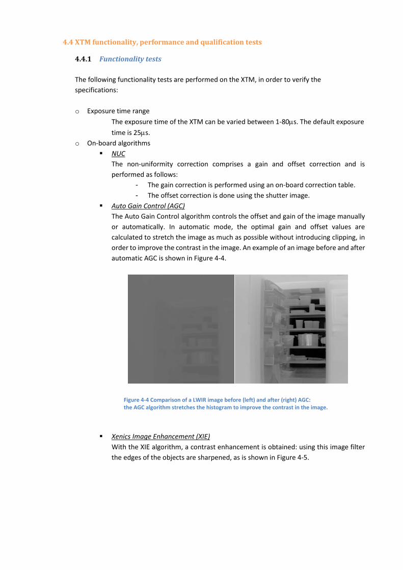
Auto Gain Control (AGC) The Auto Gain Control algorithm controls the offset and gain of the image manually or automatically. In automatic mode, the optimal gain and offset values are calculated to stretch the image as much as possible without introducing clipping, in order to improve the contrast in the image. An example of an image before and after automatic AGC is shown in Figure 4-4.

Figure 4-4 Comparison of a LWIR image before (left) and after (right) AGC: the AGC algorithm stretches the histogram to improve the contrast in the image.

Xenics Image Enhancement (XIE) With the XIE algorithm, a contrast enhancement is obtained: using this image filter the edges of the objects are sharpened, as is shown in Figure 4-5.

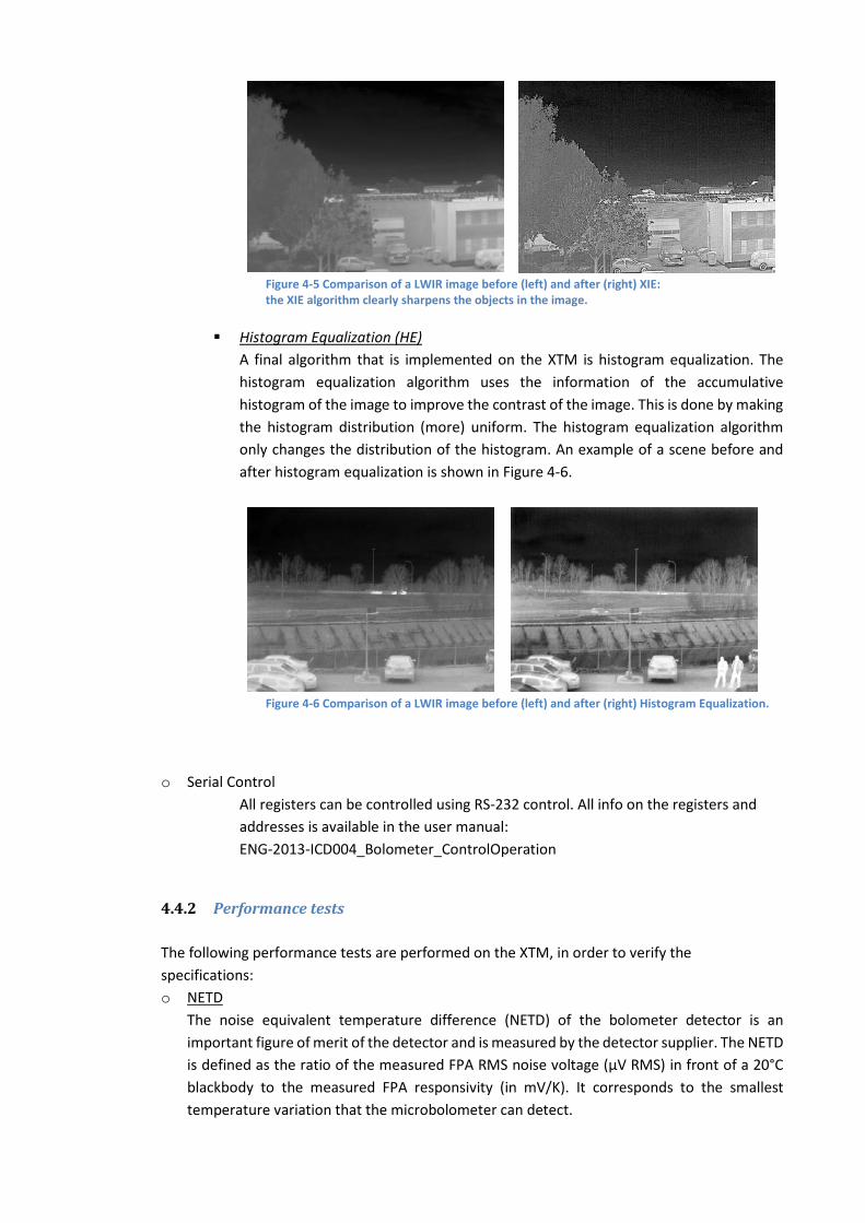
Figure 4-5 Comparison of a LWIR image before (left) and after (right) XIE: the XIE algorithm clearly sharpens the objects in the image.

Histogram Equalization (HE)

A final algorithm that is implemented on the XTM is histogram equalization. The histogram equalization algorithm uses the information of the accumulative histogram of the image to improve the contrast of the image. This is done by making the histogram distribution (more) uniform. The histogram equalization algorithm only changes the distribution of the histogram. An example of a scene before and after histogram equalization is shown in Figure 4-6.

Figure 4-6 Comparison of a LWIR image before (left) and after (right) Histogram Equalization.

o Serial Control

All registers can be controlled using RS-232 control. All info on the registers and addresses is available in the user manual: ENG-2013-ICD004_Bolometer_ControlOperation

4.4.2 Performance tests

The following performance tests are performed on the XTM, in order to verify the specifications: o NETD

The noise equivalent temperature difference (NETD) of the bolometer detector is an important figure of merit of the detector and is measured by the detector supplier. The NETD is defined as the ratio of the measured FPA RMS noise voltage (μV RMS) in front of a 20°C blackbody to the measured FPA responsivity (in mV/K). It corresponds to the smallest temperature variation that the microbolometer can detect.

For the XTM used for the SUNNY demo, the NETD from the detector test report is 48.7mK. After XTM fabrication, NETD is measured at camera level. Therefore the responsivity and noise were measured per pixel at different exposure times (10-80 µs). A percentile plot (giving the 0.5%, 32%, 50%, 68%, and 99.5% NETD pixel values) is given in Figure 4-7. A NETD of 60mK at 80 µs is obtained at camera-level.

Figure 4-7 Percentile average ADU Values of Ulis 55mK

o Power Consumption The power consumption of the XTM-640-PAL is measured, and resulted in 2.15W.

o Environmental tests The following environmental tests have been performed on the XTM:

Operating temperature range verification: -40 to 60°C The XTM was tested in the climate chamber for the complete operating temperature range. At different temperatures, the following parameters were tested:

- Correct start-up after power down - NUC and shutter operation - Power consumption - NETD

The camera keeps functional over the specified temperature range.

Storage temperature range verification: -45 to 85°C After storage test at -45 and 85°C, the camera was tested to verify that there was no degradation. The following parameters were tested.

- Correct start-up after power down - NUC and shutter operation - Power consumption - NETD

No degradation was observed after the storage tests.

4.4.3 Qualification tests

On the XTM that will be used for the SUNNY demonstration, bad pixel analysis is performed in order to verify the specifications. The pixel yield is 99.65%. The bad pixel map is shown in Figure 4-8.

Figure 4-8 Bad pixel map of the XTM

4.5 XTM field tests: first results

An XTM was integrated in a gimbal together with a visual camera in order to assess the performance in a real maritime scenario. This first test was executed at the Belgian coast under good weather conditions during daytime. Some examples are given in Figure 4-9. A second field test was done in Portugal by Inesc in collaboration with the Portuguese Air Force. An example picture is shown in Figure 4-10. These images show a first idea of the capabilities of the LWIR sensor. Further field test results will be shown in other deliverables.

Figure 4-9 Comparison visual (left) and LWIR image (right) in a maritime scenario

Figure 4-10 Field test result, done by Inesc / Cinav

4.6 XTM summary and conclusions

In this section, we have first discussed the architecture and specifications of the XTM LWIR sensor. The following tests were carried out in order to verify the requirements: - Functional tests - Performance tests - Environmental tests - Qualification tests - First field tests

An overview of the XTM test results is given in Table 4-10.

S Parameter Specification Measurement Result S 2.3.05 NETD 50 (@ 30°C with F/1 lens 48.7 Ok S 2.3.06 Pixel operability > 99 % 99.65 % Ok S 2.4.03 Exposure time

range 1-80 µs Ok

S 2.4.04

On-board image processing

Imaging correction Auto-Gain and Offset Auto-Exposure Histogram Equalization Trigger possibilities

Ok

S 2.8.02 Power consumption

< 2.3 W 2.15 W Ok

S 2.9.02 XTM-640 serial control RS-232 Connector: RJ-12

Ok

S 2.11.03 XTM Ambient operating temperature

-40 to 60°C Ok

S 2.11.04 XTM Storage temperature -45 to 85°C Ok

Table 4-10 XTM Test results

5. General Conclusions

In this document the design, functionality and specifications of the IR sensors (LWIR and SWIR) are described. For every sensor, performance and qualification tests are executed and further described, in order to verify the specifications of the sensors. Finally some results of first field tests are given to show the performance of the sensors in typical scenarios.

6. References Sunny. (2013). Description of Work.