~D-A125 ASSESSMENT COMMUNICATIONS INDUSTRY Enhsoon …
244
~D-A125 358 SOCIOECONOMIC IMPACT ASSESSMENT COMMUNICATIONS INDUSTRY 1/3 PHASE IV IMPACT A.. CU) ACUMENICS RESEARCH AND TECHNOLOGY INC BETHESDA MD 21 FEB 81 FAA-RPO-81-i1 UNCLSSIFIED DOT-FR78WRI-932 FIG 17/2. 1 L Enhsoon monsiE EosshsonhmonsoE mhhhhh 0 0hhhhhhE 0 EhhhhhhhhhhhhE EhhhhhohhhhhhE
Transcript of ~D-A125 ASSESSMENT COMMUNICATIONS INDUSTRY Enhsoon …

~D-A125 358 SOCIOECONOMIC IMPACT ASSESSMENT COMMUNICATIONS INDUSTRY 1/3PHASE IV IMPACT A.. CU) ACUMENICS RESEARCH ANDTECHNOLOGY INC BETHESDA MD 21 FEB 81 FAA-RPO-81-i1
UNCLSSIFIED DOT-FR78WRI-932 FIG 17/2. 1 L
Enhsoon monsiEEosshsonhmonsoEmhhhhh 0 0hhhhhhE 0EhhhhhhhhhhhhEEhhhhhohhhhhhE

LI
lf
*4a

4
(,umY -
*fl\.~ '4~~
~a9inin* frrti.te * ~ i111Wld,
-
___ T7T1)

Th conent of thi reor reflec neithe
aIoiinnra ffca oiyo h
frthe contents of this oturelet oruetheref
a ~ ~ ~ ~ ~ ~ ~ AM* e poiFnnoonofiilpliyorh
Departent o Transortaton. T isueti
disseminated in ~ ~ ~ r th intres of, nfr ato exhne
TheUnte Sats ovrnen asuesnolibiit
for~ ~ ~ ~~~~4 thiotnno ti ouetorueteef
Dal ,e .1 'a.
~Special

-L j &p
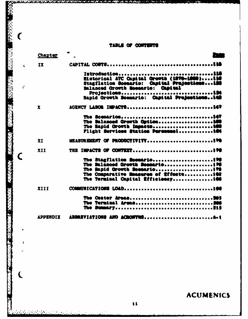
TABLE OF CONTENTS
Chapter
*I INTRODUCTION TO THE ASSESSMENT .................... 1
II NATURE OF TECHNOLOGY ...... ..... ............. *99*. 3
III FUNCTIONS OF COMMUNICATIONS TECHNOLOGY INA N AVIATION SETTING...*.. ....... .. ....... 11
Functions of Communications Technology******. 11Air Traffic Managemento..................... 12Detailed Outline of Function of Communi-
cations Technology....5 ..... * ... 22
IV GENERIC AND ANTICIPATED EFFECTS ......... o......... 59
Anticipated Efet...... . .. * .62
Productivity of En Route Controllerseoeee.... 63-'Productivity in the Terminal Controllers*.*** 67
Total (En Route and Terminal) O&M Cost ....... 60Approaches That Can Be Taken to AchieveProductivity Gains in Flight Service
Ways To Achieve FSS Productivity Gains....5.. 71Flight Service Trends ........................0 72Policy Impacts of ATC Automation:
Human Factor Considerations*****.**,...*,. 72
V THE CONCEPT OF PRODUCT IN THE AIRSPACE SYSTEM ..... 83
VI PRODUCTION FUNCTIONSo ................... 87
General Notion of the Production Functione.. 88Cobb-Douglas Production Function ............. 94CES Production Fucin...........97Summary....................... 98
VII ANALYTIC APPROACH TO IMPACT ESTIMATES ............. 99
The Use of Production Functions in
Estimating Impact Magnitude*.,**..........109
VIII SPECIFIC EFFECTS. ......... .......... ...... 1
ACUMENICS
TABI Or imT
ChaipteSI
L Ix CAPITAL COSNT. e**....o..........1
lutowloal ATC capital (WO~th (1990IS) **OtiStagflatioo Searto: Capia "rs9.eUW...13
baanedGrowt Semesart: CapitalRapid Growtb S"inaro: capital pF.ssIefin. *
X AGENCY LABOR W CI................4IThe Soemawios. 0* 0 *** 9 g** *0. 0 *go..... oeoo* .14?The Rapid GrthZs...........e.
XI MEASVREEN OF PC~VT..*.*.** ...
XII THE IMPACYOF COEYETO oo *so****** .........foe
C ~~~~The Stagflati g aro...........Iki Otamoed Growth ........... 3
The Rapid Growth ksro..........The Comarative Meassre of 2tt.....The Terminal Cpital Effielmsp....... 000.01S4
The Center A~megeegggggggg~g
The Ownuaree 0*00000000 eeegggee~S~
APPENDIX ABBREVIATIONS AND O eeeeegee...eefa
ACUMENICS

(WAL
-S ~ vim
Al
Olik 11"11 111 d . " , al o - - - -
*#I~~~~- lo *" *4 *O IW V i I Poo
a-o I"- itShk ~~~~ * -------- -
to Vale ~ " 1 00"1200"" IN40" too g mp W9k l -. 4
~ *%~ ~i,~P~4 - -dO*'

WmI %os £tTsfte sa bspWSI. m."'
to i Ini ve emie ami et am
of Ipa* On"9 Web~m ftslIsu amSpuu
004quW* .Ofe a*v~t*-t s.... 2*************** .151
mwomj.. ... ......... ..... oe0 000000 00015
%040 "Orwttf twsimmau spv"* a StatadGth~W ~ ~ . . ~~ . ~ -- .~ * w v w* OW vo ** * 0... .. . ..0 . .0 * 0 6 00
ACUMEN ICS

TABLES
Pace
,%35. Center Staff: Balanced Growth Capital, Rapid Growthand Stagflation Activity.... . .. . . . . . .. ............ * 162
36. Terminal Staff: Rapid Growth Capital, Balanced Growthand Stagflation Activity.... ..*.o..OSSe...... .. ...... .163
37. Center Staff: Rapid Growth Capital, Balanced Growth andStagflation Ac..v.y......o•........o•...........166
. 38. FSS Personnel - All Scenarios.....•..........o eo....•.o•.167
39. Balanced Growth Capital - Balanced Growth StagflationActivity.•.. 0 ... **.. *.. ..... •... .... .... •*..... ....169
40. Rapid Growth Capital - Other Scenario Activity ............. 169
41. TOPS/TERM ............................ ........... g. 172
42. Stagflation Scenario... ... o..o...o.o........o..............177
43. Balanced Growth Scenario..esooe......... e..o...........179
44. Rapid Growth Scenario. ... .... ..... .... .. .... 181
45. Impact Measures- Congruent Conditions.....................185
46. Impact Measures - Stagflation..............................186
47. Impact Measures - Balanced Growth.........................187
48. Impact Measures - Rapid Growth ...........0............ ... 189
49. Relative Efficiency - Non-Congruent Conditions .......... ..192
50. Relative Efficiency - Non-Congruent Conditions............. 193
51. Relative Efficiency - Non-Congruent Conditions..........o..194
52. Terminal Area Radar Control Locations......... ............ 197
53. Communications Data Summary......o..........o....o.........198
54. Communications Content Per Aircraft-Terminal Area .......... 202
55. Balanced Growth Center Communications Load....•.. ........ 204
ACUMENICSv

CTABLES
56. Rapid Growth Center Communication Load.. ................. 206
57. Center Stagflation Communication Load.. ... . .. ... 206
58. Balanced Growth Terminal Communication Load.°.. ....... 207
59. Rapid Growth Terminal Communication Load.*..s°*.....*.e...209
60. Stagflation Terminal Communication Load°.°.....°.. ... 211
61. Center Communication Load - All Scenarios.....°............214
62. Terminal Communication Load - All Scenarios................215
ACUMENICSvi
".C
a. . • • . . . . • . , • . - . . - . -
. . ... . ,I ml n k h -mo 4 J.- -, a, ., -a. - -. L -; -

a. contou cminI~auo W" - "1I 00
7.Twulmal C Iatso'm 3d 441 000-033 ,0
ACUMENICSTitI

6 am 40" *,-0- ;4-0 I~*
O~o w
- ~ ~ ~ ~ ~ A Im0 fam 1Wa0 ~-~- W~~
"ttMmq4w 4"W" "A "Am 4.0 4m Di
.a9 .~ 4~0 "ONe ** wSo OW.0 4o
O-"-o 000""W mo *am#~ * atmp o
t~~~~~b~~ "a w ap *4 - 4 0

4Nm ~ - S~9~. W ~lM 1 I ftwit. tobOlogy Le
~4~i44"140 9441 00S 4e towtm of the eapttal Loyost.
65*600*W ~ 1 Iof M1W ow fa te twst eaw lo
ft vqwoo G **#W 91W fl 1,0 *surmw of tbirtos
b4~164W kff meW 4404,144 5 ~ * seeml. etreestv of
Q%*~ A"I0II "e 40 4 4 .5* *~ *""I of sommtq &" the
40"w.",uIPA* &10o "W04" Ofse tM T"e rosettes of
~ I5*~6*~ W*44Wm#W & e ffto till). a
~~'*A~Ie eS*1 .45 mo* "s - - #0e ffect,* of olease
oft o4"Mmoo 104 ftPEI S0 9 ooom tbe $*swat
(4- $0w~. O"OM4 OWW O e#t*u. 1*0 1ep Lto.
~~ !* A~~**~ *W9 *S41ss s OWetles fusettess
*40 f*WMW4 *' ftMIsems% soU,1 e~n .Of teW
4SW404 0 q"0040* AN* *$, *Vko I f**~t will idestift"e
~*mouvowes ** Vg'Wf *W ~99Wj #4wo. ##* for1 ew. tt
ACUM.WE\ICS

II. NATURE OF TECHNOLOGY
The purpose of this section is to provide a basis for the
* classification of generic impacts. The creation of impact classi-
fication allows one to examine the nature of impacts and determine
the generic effects of impact. The use of such classification
schemes does not imply that one paradigm obtains for all tech-
nology. Rather, a classification scheme allows one to distinguish
among types of effects so that a priori decisions about the focus
* of this study can be applied with some degree of efficiency.
A technology can be defined as that knowledge or set of
* physical objects that allow a "want" of man to be attained. As
I.' such, the technology and the use thereof are an attempt by mankind
to overcome inherent physical or intellectual limitations. The
adoption of technology occurs if man perceives that some function
can best be performed using a human surrogate. The use of tech-
nology alters the way in which a function has been performed
previously. The non-human performance of function requires that a
technology operate. The act of operation requires the consumption
of resources and generation of by-products. The impacts of tech-
nology, therefore, derive from function and operation.
The effects of function refer to the purpose of technology
ito its societal context; such effects represent or are indicative
of the consequensces of a class of technologies fulfilling the
ACUMENICS

sow alar *seia objew"9946 Us Tofm et of Ot "rotor t anr--wam of a -- mwoo Obs"00 #Aem.
ma ba espremed a mail for Omivslg OWO4 .Seesma "we
lb. fuse10 "as e be pwww sta 6 emob of , .m w 4w.
80166104 .ini-fired per pIsie. !I**"'l an* 06mo lem
oillaf led powsr PIeSSI so ws~~ V~:: p$,is. 0 Stow"4
the fuseIO lies si0 I. 140.a " *.b ISI"II sl 04414M*041
**eda an0 .al
ib" mociI ed of eia fm~keft Ofbw tm ~I.
Opeki te10 eoalog. se"v. too Oflwi of ComrtIAM wvopY--
C PO lift *POIfIC tOosesi4" ONi "NO. NOM10 OW*t.PO.#
each teebeelog "it ""w esftmsl """to~ "s eswm Owww
reqQIrIMeI. 140 t441 t1e. of.t~~ 14 n., 4P09,%4
actwma1 or P01061161 of pfvet*, 94.0. iAm Oqtw4404 Sao.t*'O
force of *uocts *%. *netflirv po#ov*
Owartie.I efft*~ 0 *t 15 wvwmew P.w qwvo* v9.44
effOCtLS. fttt. 10 tl of VOWSIIes %*fIWOw&, *41tiw* Vf
funaioeaI ef fect** Tut it. law $V@#t#4* of * 9 .o~ 1
areitse as. 6451t of imo tt e *"wo to ~ , #*~~
SI erfrtl the~ sof Ot. gt~w wt 0pO't.* ~*99 ~
trersew~r~ INC chnne.ow*91titt ii*e *, tm,
A C U MUS-I C

Ow*5* 1116 -~4 mw *ot *0W **A%**"* w-P
Mo #1600 lo - No 4w" 40 Omwm 01 . hm~
F~* ~* NO40P. OwP -fsww 40 Soia .Off.
evomws 4* * 40 mW9W Ot
ow**. *'#+ Oo #' 4~ 00404 m00 1.~to
0009 * - "a9wu 400 Ims4W~Im oq*4* ***"to
C~*- 3 N* * 446WS95 - 4 .. Ws W40. MV P OW 4%0#4
*ew 040efrs *f OW V* IUI *4 "04 4- *M .400 VM*f4 M
~q$** * h* 0*404 &qqw'fl*9h" ~ 4 44 "0 "q9w*lq fot mwl 40-
ItP 4W T #bi4S %" p* itev *noti1 410I4 f* a*-** 1"9gno
04 -4~ *A"lq4 a . .w- q.* ImwwI .W. *91 Ii
* ACUMWENICS

9
C
I
I
ia
Ir
N
04'*
1ft I~.t .4_________________ Ii'i'_________________ 0=
I 2
h 0
S
0
S

might include: time, content, the nature of the transaction, ease
of use, cost, etc. The relationship between various communication
* technologies and process variables is illustratively shown in
* Figure 2.
1) the application of technology occurs due to the
derived demand for some other good or service,
2) the effects of technology derive from its func-
tion and being,
3) the effects of technologies having the same
function are similar in kind but vary in degree,
4) the magnitude of effects due to function vary with
the magnitude of sundry process variables,
C5) the effects of operation are due to the physical
attributes of the technology,
6) the effects of a technology due to operation are
independent of function, and
7) the operation effects of technologies having similar
physical attributes are &like in kind but vary in
degree.
While the notion of technology is complex and the effects of
* "being" vary with specific technologies, some general propositions
concerning machines can be stated. It should be noted that the
* statements derive from the use of the technology (i.e., turning on
the switch) rather than from fulfilling a societal objective. In
this respect then, technology in use has the following results
ACUMEN ICS4 7

q00.9
C4
d d 3 C
L4
c
0
x 4
z a
944-Qx4CL
4"4
-P 00 0. as st 410
0.e -fNIN0W)) Z W Xn. ... U =6 l XW

* attributable to operatlon:
1) it serves and specifies, sat" or "om"a"m,
2) It yields a product or oe1vtow,
3) It is self-consualms
* 4) It consumes energy.
5) It consume resoroes for lbe pr aemu@
of a good or provsion of a ssryte.
6) it smits excess enrgy
7) It causes nolse,
8) it nay cause air pollution.
9) it may Influenoe the eolo3,
10) It employs/displaose labor,
11) It substitutes for amotber teebmoloW.
12) there is a risk associated with oper tles-
i.e., non-operatios, structml filure,
Injury to labor.
, Each of thece Orosults" ca be treat" "s varlabl e es d, to *oft
extent, be masured. The speific variables aselat.d itib mab
result include:
Result na""It serves a specific social sf* f* tsetls.or economic function.
It yields a product or ideatify prIV t qt qv"tI.service.
ACUMENICS9

aim
* # f uso eaal 440" o -p*4 4*
$0S 40M Off 0040O qIa -wom~ b~ ~ - au6in p4
iP~~wfvq of - h-s
V* 410 1~~
*~~~~d O *w ,.- OONO. SUA
S~b*4A4 c u4m"Icl

* 4* eof.t so" inC* -1 hV Ofest" for oYatteme1
- fqm* #$wamses e* "ite Oit is tatocies of am.
"04004-ows Iis 060 ;q noo *"A t Ea.divs of Labor
#ww *WWI, oft #Wvmt w m of £6 A" Ia.tee " wall
Fr~ft ## It 0* NOWR ft oemlf am Othe ti totss of
NOW 40 #to. Otft.
09OMW of tel iS0 I1t t Is deety No OSUII£6 the 11,1017
*bq~s00* a*Dwmk 01 MW **R1OO b~mtimge t~ocheOIag. to
"*t *Mo Of .9e *" s~ Vto" gill to iwtO4. such
04014fp too .*#lo OW Ot piltots a" Si ftrft ower is.
~w~'a *.i #e,,tis, to*" *00 total evreie Carrier,, Comuter
*~e~too, t.*I Ott. te nme r t h airspac
*~ ~l i IS ~ sto aer~ 1late due to the sdoptlon
'~ tP'#I?,I*~ tW ,WK- gi4#w Ifoset elefe ttri PAA operatious
ACUMENICS
The effects of new technology will derive from the functions
performed dhd/or needed by airspace users and managers. The
magnitude of effects will depend upon the extent which new tech-
nology usurps existing or creates new functions. Therefore, to
examine these effects one must identify functions requiring or
compatable with the new technology. This section of the report
will identify the airspace manager or user functions attendant
to the National Aviation System.
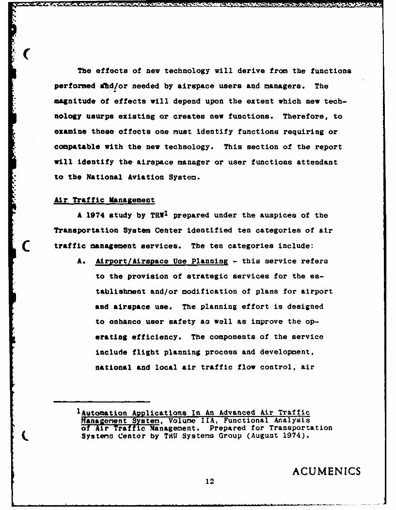
Air Traffic Management
A 1974 study by TRW1 prepared under the auspices of the
Transportation System Center identified ten categories of air
C traffic management services. The ten categories include:
A. Airport/Airspace Use Planning - this service refers
to the provision of strategic services for the es-
tablishment and/or modification of plans for airport
and airspace use. The planning effort is designed
to enhance user safety as well as improve the op-
erating efficiency. The components of the service
include flight planning process and development,
national and local air traffic flow control, air
1 Automation Applications In An Advanced Air TrafficHanaaenent System, Volume IIA, Functional Analysisof Air Traffic Management. Prepared for Transportation
( Systems Centor by TRW Systems Group (August 1974).
ACUMENICS12

traffic conflict prevention, efficient allocation
o16 airspace through planning, and the flight clear-
ance process.
B. Flight Plan Conformance - the purpose of flight plan
conformance includes the tactical effort required to
implement the airport/airspace use plan. This includes
direct discourse between airspace users and managers.
The components of flight plan conformance include;
monitoring of air traffic activity to determine
deviations from the extant plan, definition of actions
necessary and implementation of corrections to the plan,
- ( modifications of the plan, monitoring air traffic to
identify conflicts in the airport/ airspace use plan,
identification of and inplementation of actions to
ameliorate conflicts.
C. Separation Assurance - separation assurance is a
tactical service designed to improve the level of
user safety in airspace. The service includes
conflict and collision prevention. Tactical con-
flict prevention includes the following c'x.iponents;
monitoring and predicting violations of specific
airspace. Tactical collision prevention includes;
monitoring to determine actual violations of airspace
C and resolution of airspace violations.
613 ACUMENICS

:-",
D. Snace Control - speM ostr IMo1lsoo tGelsa Ote qftes
disignod to Increase the effleest so of avatbW at-
space. The camposents of spactmg ostrol testslee rus
configurations scheduling am allOsattOi of r i *at~
for takeoffs and landlags; the dktemltLea @f tbe ap-
propriate sequence of aircraft for WaLdiug. akesie sas
on route movement; and idetifioato and adJstmet of
separation distance among aircraft.
E. Airborne. LAndinc and Groumnd Navicatis - this servlI,
identifies and defines the location of aLrcraft at a
discrete point in time.
F. Flight Advisory Service - this service provides is-
formation to the pilot during all pbasee of flight.
The information provided includes data conernisg
weather, air traffic, facilities, routes, obtructiose
and procedures and regulations.
G. Information Services information services provide
pilots with a variety of data during pre-flight
planning. Pilots may obtain information about
weather, air traffic, facilities, routes, obstruc-
tion, and regulations and procedures.
K H. Record Services - record services include the actions,
- L events, and documentation necessary to permit operations
rocord3.
ACUMENICS14

#WO* 4. ,m. 40 * qm 4
*to lit" ___ _. * -0AP~ 0"
0 N$04" a"W " P444SMS
tie it6"04 4 *414" t"0* p - h * * ~4404esSa
9SU to ,S.4 m e". fmkv.~* IF+ "4441"01 4"" ""K.
'4o "hYA91fi't riefw tto -a 4olli
S. ~.&m.i A ~ ~. j~g.y~&JAV W~4

~e ~4 43. m4e t&"oM* 4A* OVA4Mm 40W
'n ~.ggsmum Esaa P40m *pe . 4000 419t*l
.&et fl *4W s* n"eaAee914O an 40 fms4
bt sojg 4bftslft' t % p ** o
"'%ftowrw * * * -to kqfl9.eoso.f 4 1% *0P Q4l p% 4J~j
U tO * 40 b 9 i
.~ p.p* %qqn4~ ~ at nr * n~q~neq 40.0
mA tY'.9W*1 ~-r'n -. 4 P - t t p~s ~~al I
40.P~- .4'ffV; r-''- - b to t. two

0. Maintain Conformance to Flight Plan Tb.
pdrppe ot bis function is to monitor whether or not
as streraft ts being ftlom I conformance with the
fligbi plan. Actual and predicted deviations from the
fllgbi piss are evaluated. Actlons are Loplemented
to correet 1 -9% ettuatioem caued by flight plank~*9 tol g I *as.ll
. J " A re lparatiO*e of Aircraft - The pur-
mo of iIt teetllla to to predict and aseliorato
I**Iue ocefieta betesm aircraft.
t. Ontf . o ateg or Aircraft - The pIrpow
e l %*i, twmioe I* to lwwe, asa s eule aircraft
.~ *1 e~t as* of Sirep.. aM factitlt .
'* ~JIaJ a ft POU141~V0.er L&Odi.4. sad Qr9%*
!* jII ~~ql* 94l o 4t owe 40(Irlllil lmI
b 1. .rl! 4 11e ci to pto Vii. " 4
• + j* fi s I. , tt. 14 *'It+f tf S 41*-
A t Mt? lCS
-amm mmm mw

efr~dIomts 44 mee ptre %slw W"i Owt# i
1ia os to 1@ uu.ter 1&0. roop"aIftlls tow fmmmw.
costi of Stmrall frws no Sir tvOfti'
(AT") jorio4icties to oe.Uso
14. 94161610e *%to - ill *lu rti' .rjwuw
of vrsts rosettes Sl to It OW10a *to"rw *-
C Spw~a osoe *wltotIt.. t r..rt..w61AN
0. ruacion 15 - PrOVIACS AW'111t~ 0* *PONt-#O bjwmt £
Thp purpo. of thio fSAW119*t I- ofWof I#q do wrofm"%i
manuals.
P. rbufct10* Is - p'-4ide Put* -tt~SA7%
pose of this ruwtia" 14 to, PtI. 0v4et
services to tNw evet 1 to*' at i~pli v~tiuw
Q uflction 17 - adiVai* ar*10i-* CA401ii1 0*4 st-at"
maintain a Curre~t 410'Abese 4e'sCti1~i*z 1+00 st-SIws
(ani Capabilitl 91arsa!e
A C U MNIC S

fewl~~~~~~mma4#~~.- *wwal"S. 44% m 0 100at w
for~ on of t~w 6a m too-#
... uA"* fs*Iiq" Ott 4~I 11. olw S1o. Ossri
So44 4w@ VI a some *Ift 14w-i bSwim 60IM@
i* **~4h iS*011W qwlwwt le t ittr er
* 4 * 2" r' rehit#4 it up I~q~istovt
ftv Al**t tof~~*~I te Iperforse
-f.t ,f.A-#j* 4f-i* ~It*t **1jI* itllr&**f e e UP iler
s~t~~' t , s ifi~l *0101 ql*0 s fct,3up imtIs
ACUMENICS

s Mon cmv~l
7. if nwaa *Mmum MA IMK
6. .w.aost M
0. u 1 att MA KI
10 %MIMS comfKM
9.amvi u o a~11t M
10. orcwu* aLuftt" KMK DA I Ku&mmms
13. Prst aKMw KD M IDA IK D
14. WAnut um uma KIDJ:: lf Pwdaau &K I KI I IDA
17. wftn~ tumca.-- K I IVWalt % sutaim
t I ntrstion
t. frogre for Tranuortatiol System Center,W7 M~ ThyStuu qP 1974. (Cbntract tb. -TSC-512-2a)
03

N.Nib
U) N. Il . 3
Ilk
N. .
NNu
N. N. ~. A N
in c t
21N
7(7 7777
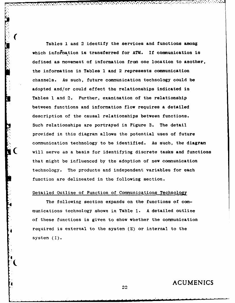
Tables 1 and 2 identify the services and functions among
which infol~mation is transferred for ATM. If communication is
* defined as movement of information from one location to another,
the information in Tables 1 and 2 represents communication
* channels. As such, future communication technology could be
* adopted and/or could effect the relationships indicated in
Tables 1 and 2. Further, examination of the relationship
between functions and information flow requires a detailed
description of the causal relationships between functions.
Such relationships are portrayed in Figure 3. The detail
provided in this diagram allows the potential uses of future
* communication technology to be identified. As such, the diagram
C will serve as a basis for identifying discrete tasks and functions
* that might be influenced by the adoption of new communication
technology. The products and independent variables for each
function are delineated in the following section.
Detailed Outline of Function of Communications Technology
4 The following section expands on the functions of comi-
munications technology shown in Table 1. A detailed outline
of these functions is given to show whether the communication
4 required is external to the system, (E) or internal to the
system (I).
4
e ACUMENICS

O3D
(Page I of 2)
Source: Autmtic A0wlicatim.s In OP Advncd Airafic Man nt21. Vol. 1 -.
FciolAalyss o Aft Traffic lot.Prepared for transportation System Center, 001by TRW System Group, 1974. lContract, No.DOT'-S-2- 2a
23

- --
SW4Wi *0 a
f~t~ti~ tfti~i* 4 im lftffi
ptmot fie*MW or
" "a lft~r1911S
24

4. ftmt gusa Mobsia Mlases
1*09~oaltos
WS4*44 prqlgw.
*. w4.f" lp$ssPess
Lim~ ,
0%** toums 14 of T#04s
*.#rne'NICS

%_%*.
Comnmunicat ion- Required
2. Independent Variables:
a. Erogenous SourcesFlow control paradigmTime Stimulus EList of Terminal Jurisdictionsin ATM SystemCommercial Schedules E
b. Pilot Request to Establishor Cancel Reservation E
* c. Maintain System CapabilityI(Function 17)
C. Prepare Flicht Plan
1. Products: E
Ca. Cancel Plight Plan E
b. Submitted Flight Plan
*2. Independent Variables:
a. PilotDecision to use airspace intentions EAircraft capability and statusStatus of Onboard EquipmentPilot QualificationsAircraft Identification and Type
b. Issue Clearance and ClearanceChanges (Function 5) E
c. Process Flight Plan (Function 4) E
od. Maintain System Capability (Function 17) 1
e, Exogenous SourcesFlight Plan Form~at EConsistency Checking Paradigm E
ACUMENICS20

Comimun icat ionRequired
D. Process Flight Plan
1. Products:
a. Intended Time position Profile Ib. Priority of Proposed Flight Plan Ic. Inform Pilot of Flight Plan Approval Ed. Inform Pilot that Flight Plan must be
Changed Ee, Accepted Flight Plan Ef. Cancellation of Flight Plan Eg. Define Communication Channels E
Between Aircraft and ATM Systemh. Special Services Required E
2. Independent Variables:
a. Maintain System Capability (Function 17) Ib. Control Traffic Flow (Function 2) I
1. Terminal release quotas2. En route jurisdiction release quotas
c. Submitted Flight Plan (Function 3) Ed. Monitor Aircraft Progress (Function 6) I
1. Correlated position and identi-fication
2. Predicted long range tine-positionprofile
e. Maintain Conformance with Flight Plan E4 (Function 7) -Proposed Flight Plan
Revision
f. Control Spacing of Aircraft I
1. Proposed revised flight plan
g. Provide Ancillary and Special Services E
h. Exogenous
1. Approval criteria
* 2. Priority criteria
ACUMENICS27

communicationReauired
i. Pilot
1. Acceptance of Flight Plan
2. Request for Flight Plan cancellation I
E. Issuance and Changes in Clearance
1. Products:
a. Proceed to Alternate Eb. Request Approach Ec. Flight Plan Tolerances Ed. Vectoring Requirements Ee. Transmit Clearance Ef. Unable to Issue Clearance Eg. Issued Clearance E
2. Independent Variables:
a. Exogenous Sources
1. Identification code usage procedures I2. Time stimulus3. Identify Code Paradigm •4. Terminated Code Assignment I5. Clearance Format I
b. Control Traffic Flow (Function 2)
1. Terminal Release Quotas I2. En route Jurisdiction Release I
c. Process Flight Plan (Function 4)
1. Accepted Flight Plan
d. Monitor Aircraft Progress (Function 6)
1. Long range predicted time-positionprofile I
2. Correlated position andidentification I
3. Readiness of aircraft E
ACUMENICS28
mm
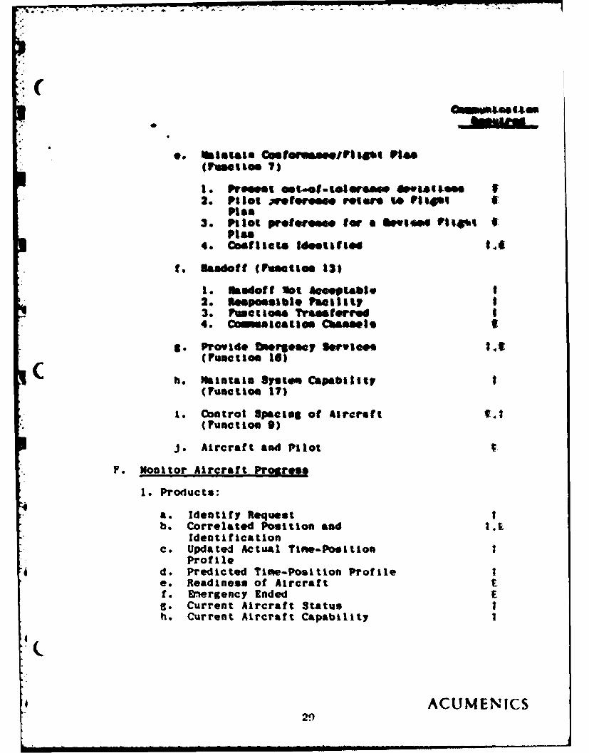
(7u6ites 7)
1 . PFy.I R.@st-io1rS teI . I2. Pilot etferew mtr@ toe P*to
3. Pilot prtoereeo for e fiewtoW Wli1t IPlea
4. CoofllG94 ldoeatlft|.
f. nasdotf (Pisettim 13)
I. kedo t ft 4e O9ale I2. eepossible ftwility I3. ?%motioe ?vaastef I4. iCma AatI basele 10
S. Provide urseocy Sowelo(Function 16)
h. kiataim $"sto capability I(Fuaction 17)
1. Control Spacing of tlrarsft 1..(Function 9)
J. Aircraft and Pilot
F. Monitor Aircraft Progreoo
1. Products:
a. Identify Request Ib. Correlated Position and I t
Identi ficationc. Updated Actual 1itw-Poition I
Profiled. Predicted Time-Position Profile Ie. Readiness of Aircraft tf. Ehergency EndedS. Current Aircraft Status Ih. Current Aircraft Capability I
0 ACUMENICS29
k- II llNi l a S a ie

*1
(wRt.44 e**
4., &M~mflb* Iqataa
4 ~t4~i4SIS~
t *t&s. 44'4~ sse'* 4 * *** asd 4-*M~&4~4Uc*W~ flW4* *
* **4S MS''4O* *4**44409..* fl4* *
* t..A'fl~D4 .ehs'4 a.* I* *i'. SD - &..eqmp,~.s 4r
* fl'.s.mmw dLtrt fl4* t*WW.44.* a
% 344,** *4~4fI 4kb44 40* ~4~s 4I. *..~e 8~+d** 449* 1 .1'
& ~ flq4fl tb*64I0I1;444 ('W4~e4 #4m* 4 i
9, t~
( 4+ *~4~s~4#4
4. %~~AA*~k~t lnttsSten M1A~ SiAn fl.m
t *tI~4'%4 *Z9* ,f. bt*t7*4 #4S q0~44 t
*.. tsn*~~.4* ui#s*~*t~ 4* ;ri~*** tn$ *jr.*~*q $40t.r,4* 1
~. *r.rw*9 fisC' *PI*. 4.a'*$.4.* t 4 a~,,fl S&4 Mt*f?~&4*' t
0., ,;I; ~S't-j9~1 *fl* '.t t I *isP
~.n ~ a
q tWt4 ,&j~ M#: tt ~tte '*# 4 *I*
0(
* AcjrqtNlrI

400 640 4WA. f54WI14& 4 .
4~~ W'. 4^ tR4 *,I&.~444~ a' 4 .*N 4P A
*~~46 4 4- -*'4 4~4U 4~4e

3. Loog-term predtcted tim-positteeprofile
4. Correlated poosittoo aad idot1-fleet 100 1
d. Provide ergescr Serice (Nectioa 16).
1. awrgeoac flight pIS2. Revised swergeocy flight plea3. werency eede,4
o. Pros eaogeoous orce
1. Time stisalus2. System capacity to pertome Fsacttio 7 I
f. from aircraft
1. Statewnat of preferece for carroctioeback to flight piss 1
2. 3tatuemat of prefereae for reisioqof flight plan C
S. mintain syst"I Capability mad Statvt IInfornatloo (Uuectios I?)-
1. Active flight plan coust
HI. Assure Seoaration of Aircraft
1. Products:
a. Nigh invinence conflict paire Ib. No action required Ic. Careful nonitoring required Id. Perfornance correction require, 4e. ?ransmitted performanco cYango
aessage tf. Transmission required tg. Revision required (of perforfabce
tessase)h. Revision not requirel Ii. Action classification uplated I
ACUMENICS32

(Cinmaacattoa• AeauLrad
3. ~ede t Variables
* Fro OnPewO osroe:
1. ?Sm sL, uml3. OottiatiOa of airspace volms
for oefliot detectlon t3. b0tisatio4 ot IUs intervals
for oeflict detection I4. petih probability paradigp IS. Opiate @lrae tw
S, .io4r Alrrraf Progross (Pnctlon 6):
1. Preio4ted sbort-rasge WIn-poelilo tprofile for the aircraft
2. predicted long-range tiel.-po41tIonprofile for te aircraft K
3. Current aircraft capability (Includes( perforsese capability sad user class) I
a. Provide Acillary sad Special Services(reaction 16)1. Iffination of special separation niania I
2. Special service so loner required I
d. t'Frn the Aircraft.
I. Aolsoledtent (of perforance change
e. ftnitais Syoten Capability sad Status|sformatios (Fection 1?):
1. Stored databas St (rules andprocedure s-4ilfnum separation tstaftdar4s)
f. tswe Clearaoce anI Clearance Changes(tuecttoft 5)
1. Clearance Issued £
ACUMENICS33

CommunicationRequired
o
I. Control Spacinz of Aircraft
1. Products:
a. Acceptable distribution (spacing notrequired)
b. No ETA/ETD changes required
c. Performance necessary to implementsequence change I
d. Revised flight plan E
2. Independent Variables:
a. Control Traffic Flow (Function 2):
1. Terminal/jurisdiction total demand(I as a function of time I
b. Process Flight Plan (Function 4):
1. Priority of the proposed flight plan I2. Accepted flight plan I
c. Issue Clearance and Clearance Changes(Function 5)
1. Flight plan tolerances I
2. Request approach E
d. Monitor Aircraft Progress (Function 6)
1. Predicted short-range time-position Iprofile for the aircraft
2. Predicted long-range time-positionprofile for the aircraft I
3. Current aircraft capability (includesperformance capability and user class) I
I (
I 34ACUMENICS34

CommunicationRequired
e. Maintain System Capability and StatusInformation (Function 17):
1. Stored weather sequences I2. Stored weather forecasts I3. Stored database items I
(rules and procedures - minimumallowable separation), (groundfacilities status)
4. Stored user class database items I
f. From exogenous source:
1. Baseline capacity I2. Time stimulus I3. Criteria of excess demand and slack I
J. Provide Airborne, Landing and Ground NavigationC. Capability
1. Products:
a. En route navigation signals Eb. Landing navigation signals Ec. Ground navigation signals E
2. Independent Variables:
The specific inputs are a function of theAimplementation chosen for the navigation sub-
system but consist of some form of the follow-ing from exogenous sources:
a. Geographic location of the nav aidb. A time referencec. The navigation system structure
ACUMENICS
35

Note: The airborne, landing and ground navigation serviceprovides a position location capability which isavailable for use by the aircraft. It does notdetermine an aircraft's position, merely providessignals which may be used onboard the aircraft tomake that determination. These signals are producedand transmitted by the equipment. Their productionplaces no demands on the "controllers." This resultsin the "function" which produces that service beingconsiderably different from the other ATMI functions.
This function does not utilize inputs produced bythe other functions, nor produce outputs used bythem. It does not require a series of ,an-machineinteractions to produce the service provided.
There are, of course, monitoring, calibration, andmaintenance tasks which must be performed. However,monitoring to determine if the function equipmentis operating properly has been included with similartasks in Function 17, Maintenance System Capabilityand Status Information. The nature of calibrationand maintenance activities are a function of systemimplementation. They are not generic air trafficmanagement activities. Therefore, the analysis ofFunction J has not been extended to the subfunctionlevel.
Communication
Required
K. Provide Aircraft Guidance
1. Products:
4a. Vectoring not required Ib. Transmitted vectoring message Ec. Responding as commanded Ed. Not responding as commanded,
retransmit Ee. Not responding as commanded,
4declare emergency E
2. Independent Variables:
a. Monitor Aircraft Progress (Function 6):
1. Correlated position and identification I
36 ACUMENICS

b. Maintain System Capability adStatus Infonatiom (FuMolios I)
1. Stored weatber sequesoee I2. Stored weatber forecasts3. Stoted severe weather ptomea
data I4. Stored database Items (fligbt
hazard inforematton) I
c. Provide tergeso, Services (Famotion 16)
1. Description of guidance assistasc*required 3
d. Provide Ancillary and Special Servioee(Function 15):
1. Description of guidance aseistasce( required C
e. Issue Clearance and Clearance Chaage(Function 8): C
1. Vectoring requirement
f. Provide Plight Advisories and Isstruction,
1. Vectoring desired C
S. From Aircraft:
1. Vectoring request C2. Heading3. Airspeed4. Vertical speed
h. Prom exoqanous source:
1. Vectoring nessage fornat £
ACU MENICS17

I.Pv. 4640001 - so of s tot r*00
0,4 tsIi i * IS. stfe'"44 T"000 004 el*.tet
%*tsees~ d ipea"W , ew w
aiof 4004IO t*0P I-fnnl
. Stw "mM 441rg £
fte ft eebav I~ to"2. tlem *ae O u"Wrn v
thatart to tfilWt 14fonotls)(OW46SA4? *"tooI et~
S.Ite"A0i ttltio 6414 1*. #ter isot *I~U &s Iikm o
q* cl.ttIi1191S.
1.#% P. - it* t**te 4le,
ACUMEN ICS

on. ~ lati posiuoe M tdoett.ticallem
2.w~l-rs Predicted two-poeIttieprfl for the aircraft
I f pmem f rest
I. 4ce ~edfamst seem** forest3. fligat adviw-y disribettom paradq. a4. Motory priority diotribatiom
6. Meft mies. fonalt 90. Tnes etISISOl 9
0. Pro* to* a IrorfI
( . Pilot Istonatioe request esma. 92. ftlot$* respo I3. So *retSoin
f. 060trol ?"'trio ?to* trwictioe 2);
1. Temleel gola~ys
6. Po*'14. 40cill"p &ad SPeOCla Serve
1. Owwrptio'S of rhequired adviories
6. Provide 6wmeatyc Sertac (FunctionI 16)
1. awsetiptige of required tebUalC&
&. OrtAwd-t*-igcavAd S&4off not requiredb. Noi-.godgosdt-l handoff
t"qu i ed
39 ACUMENICS
CommunicationRequired
c. Handoff not acceptableI* do Functions transferred
*. Responsible facilityf. Communication channelI
2. Independent Variables:
a. Process Flight Plan (Function 4):
1. Accepted flight plan I
b. Monitor Aircraft Progress (Function 0)
1. Correlated position and identification I
c. Maintain System Capability and StatusInformation (Function 17):
1. Stored weather sequencesI2. Stored weather forecasts I3. Stored database itemsI
(rules and procedures)(airspace structure and jurisdictionalboundary information)(airspace restriction information)(hazards to flight information)(COMLI-NAV system status)
4. From exogenous source:a. Pilot's request (for ground/air
handoff) Eb. Assignment paradigmI
4 c. Time stimulus5. Control Traffic Flow (Function 2):
a. Terminal release quotasb. En route jurisdiction release I
quotasI
N. Maintain System Records
1. Products:
a. Operational report not requiredI*b. Completed statistical or special reports I
* ACUMENICS40

CommunicationRequired
2. Independent Variables:
a. Process Flight Plan (Function 4)
1. Accepted flight plan I2. Cancellation of the flight plan E3. Communication links to be used
between aircraft and ATM system E
b. Issue Clearance and Clearance Changes(Function 5)
1. Transmitted clearance E
c. Monitor Aircraft Progress (Function 6):
1. Actual time-position profile I2. Current aircraft status I3. Current aircraft capability I
d. Maintain Conformance with Flight Plan(Function 7)
1. Conflicts identified by location,
time and aircraft involved I
2. Closed flight plan E
3. Present out-of-tolerance deviationsfrom flight plan (x, y, h and t) I
4 4. Short-range predicted out-of-tolerance deviations from flightplan (x, y, and h) I
5. Long-range predicted out-of-tolerance deviations fromflight plan (t) I
6. Statement from pilot that he preferscorrection of performance in orderto return to existing flight plan E
7. Statement from pilot that heprefers a revised flight plan E
ACUMENICS41

CommunicationRequired
e. Assure Separation of Aircraft(Function 8):
1. High imminence conflict pairs I2. Performance correction required I3. Careful monitoring required I4. Transmitted performance change
message E5. Transmission required I6. Performance change revision required I
f. Provide Aircraft Guidance: (Function 11)
1. Transmitted vectoring message E2. Responding as commanded E3. Not responding as commanded, retransmit E4. Not responding as commanded, declare
emergency E
g. Provide Flight Advisories and Instruction(Function 12):
1. Transmitted preformatted message topilot E
2. Transmitted spe-ially formattedmessage to pilot E
3. Transmitted message (severe weatherwarning) to pilot E
4. No response (to severe weather warning) E5. Vectoring desired E6. No vectoring desired E
h. Handoff (Function 13)
1. Responsible facility I2. Functions transferred I3. Communication channel I
i. Maintain System Capability and StatusInformaion (Function 17)
1. Stored database items (rules andprocedures) I
ACUMENICS42

Co"mutoatLato
.J. From exogenous source:
1. Classification paradigm K2. Database form and format criteria I3. Database storage paradigm4. Operational report information K5. Additional required Information
(not in database) E6. Request for special report I7. List of stored formats available I8. Recurring reports schedule I
0. Provide Ancillary and Special Services
1. Products:Aa. Special service no longer required E
b. Cease action because of safety Ec. New flight plan priority Ed. Definition of area of restriction Ie. Description of guidance required Ef. Definition of special separation
minima Eg. Description of required advisories £h. Description of NOTAI requirement Ei. No new flight plan priority required EJ. No area of restiction required Ek. No guidance required E1. Special separation ninima not required Em. Advisories not required En. NOTAM not required E
2. Independent Variables:
a. Process Flight Plan (Function 4):
1. Special services required £2. Priority of the proposed flight plant I
b. Maintain Systen Capability and Status(Function 17)
1. Stored database items (rules anJprocedures)
ACUMENICS43

1,57*0r0mtic4 fe 06444 *
P. Pro I asi.~ UV9 II q q
*.rpto 'wrqq~ v~s-In4 0*4i1*
I t ftWti~ *** t 1. O" 4 W**p**ri i
fte"Mt
A CU MEIC S44

~~*w 0 *;.qwu'n
lb* 4"l o opr
- ~ ~q*.. u~41
~~~~~~~~~ CUs MEW I4eeSINf4sbIC4I*

ComuicatLonAeautred
b. Maintain System Capability and StatusInformation (Function 17):
1. Stored weather sequences I2. Stored weather forecasts I3. Ground facilities status database
I tem
Q. Maintain System Capability and Status Information
1. Prodacts:
a. Weather observation report not required Ib. Request for PIREP Ic. Transmitted weather observation report ad. Purged data Ie. Stored database items I
(rules and procedures)(airspace structure and jurisdictionalboundary information)(route information)(airspace restriction information)(flight hazard information)(COWIf-NAV system status)(ground facilities status)
f. No change in status Ig. Stored user class database items Ih. Active flight plan count KI. ETA's and ETD's by destination and origin Ij. ETOV's by jurisdictional boundary Ik. Stored traffic data t1. Preformatted data module not required Im. Printouts (NOTANS) In. Voice tapeso. Electronic displays Ip. Stored weather sequences I
ACUMENICS46

Commitcat teReuired
2. Independent Variables:
a. Prom Exogenous Sources:
1. Time sttmulus2. Weather sensors data3. leather observation report schedule4. Weather observation report criteria5. eather transmission schedule6. Position and movement of severe weather
phenomena7. Weather sequencesS. leather forecasts0. Weather charts10. Weather route summariesIt. Rules and procedures change Information12. Airspace structure and Jurisdictional
boundary change information13. Route change Information14. Airspace restriction change information15. Hazards to flight change information16. NAV equipment status17. CON equipment status18. Ground facilities status19. Pilot qualification changes20. Aircraft capability changes21. Avionics changes22. Event counting criteria23. Preforuatted data module criteria
b. from the aircraft:
1. PIRCPS2. NAY equipment status3. cDOM equipment status4. Ground facilities status
c. Monitor Aircraft Progress (Function 6)
1. Correlated position and identification
d. Process Plight Plan (Function 4)
1. 4ccepted flight plan
ACUMENICS0 47

e. Maintain Conformance with FlightPlan (Function 7)
1. Closed flight plan
f. Provide Ancillary and Special Services(Function 15):
1. Description of NOTAM requirements2. Definition of area of restriction3. Description of required advisories4. Special service no longer required
* The preceding section delineated the components of each function.
The critical factors or performance parameters for each function
* are shown in Figure 4. Any system construct should consider the
C variables identified in Figure 4.
ACUMEN ICS48

PWLMOURM PARAMMM~t
Fun -ctI iio ..%.. Produc ...co n %w. ?. .. ..k& -racy city Wtit _ty i dlit ity| um Wie
1. Provide Flight Plan
Informtion IA x x X X X X
2. (ntrol Traffic Flow IDA x X X Xoa
3. Vrer% Flight Plan I X x X x
4. Process Flight Plan DA X X x X x X X X
5. Issue Clearance andclearance cbages MDA X X X X X
6. monitor AircraftProgress D x x x x x
7. Maintain Confornanceuivr Flight Plan IDA X x x x X
8. Assures Separationof Aircraft IMA X X X X X X
9. Qbntrol Spacing ofAircraft IDA X X X
10. Provide Airborne,landing & (roudNavigation ability IDA x X
11 Provide AircraftGuidance IMA X X X x x
12. Provide Flight Advis-ories and Instructions IDA X X X x X X X
13. Handoff IDA X X X x X X X
14. W.intain Systes( Records IDA x x X X X
15. Provide Ancillary &Speia services IMA X
16. Provide f8mrRo.yServices IDA X X
17. P.inta.n SystemCapability and StatusInforvation I X x K x K X X X
FIGURE 4
49

Pilot Functions
The atitached Tables 3 through 8 examine the major functions
performed by pilots. Related functions are grouped into six areas:
Flight path controlCollision avoidance
* NavigationOperation and monitoring of
aircraft engines and systemsCommand decisionsFlight documentation
*It should be noted that in the above construct some functions occur
in more than one area. Also, a function in one area may be con-
tributory to a function in a different area. Basic pilot functions
and other factors are using IFR air carrier operations as a paradigm.
* Other, less sophisticated types of aircraft operations may not
require every pilot function listed or they may be performed in a
different way.
In determining and evaluating the effects of future technology,
the need for communications is derived from the need to perform
the pilot functions that are delineated in the attached tables.
* Even though the literature describes communication as a separate
* functional area, it is not considered a basic pilot function in
* this report. Rather, communication is viewed as a necessary means
to perform a basic function. This method permits one to analyze
communications in the context of functions which must be performed
in flying. In this way, one can identify which communication
technology may be appropriate for performing the basic pilot
functions more efficiently.
50 ACUMEN ICS

(Communications functions, as currently performed, are LdentL-
fled for each pilot function. Functions contributing to basic
pilot functions are also shown. These identty other elements
* which infringe upon the need for communications. Controlling
elements associated with each function identify the methods for
performing basic pilot functions. As such, controlling eleneats
serve to define the structure of the current communications flow.
New technology can alter the structure of communications flows.
In fact, this must occur so that basic pilot functions can be
performed more efficiently.
In the attached tables, communication functions are describd
( r as either internal or external. Internal communications (denoted
by "I") are defined as those that occur within a particular system,
i.e., an aircraft, an PSS, an enroute ATC Center. etc. Internal
communications flows are described as either man-man, man-machine,
or machine-machine. External communication functions (denoted by
"E") are described as those which occur between systems, I.e.,
one aircraft to another aircraft, an aircraft to a radar scope,
a pilot to a controller, etc. The same descriptions are used for
external communication flows as are used for internal communication
flows.
In assessing the potential of new technology to permit flight
to be accomplished more efficiently, one must examine the communi-
cations requirements attendent to specific pilot functions. The
ACUMENICS51

eu of mew te boolop a* altr te elemts teed to Um curreet
01ounualcottas flow. For .ate, a ma,-se tise flow ay be
cooverted toe eaechlmambnb flow through auoatLo.
be data i tihis e tion ildioatee that the atrspace
mwagetwat and aircraft operatios have gsittloaat ocsmim atLow
caopmets. Is particular, aropace mneagement Lo priarlly a set
of connuncattoo tuacttoes. As suc%. cowuusicatLoo tebology to
the coaleat of the asesment offort to the entire 0"lea of
agency capital. ?bat Is, functions previously performed rstog air
to ground tole* cos uications coupled with pilot med oowtrollor
ju4onemt, have boom replaced by technology to some etoet. The
( technology Improves the accuracy of the Inforematio, changes the
nature of the Information trsmterred. alters the location of the
Information teimal. but does sot change the sod for iaformatiom.
The now stock of cmimusication technology will alter the
efficiency of agency capital. As such. it my shift nore
camuncations functions tram nan to aac le. Nowever. such
cofnunicatloos functions will remain.
* ACUMENICS52

a Ii
~I
53

, . -. -Co W w.-.. .wr.-- w r.. ,. w
0 # .' .. ad V d
5L4
IIN 0. L b b .
I3c'1 00.11 0.1!1 hi ~oi
45
- - - - -- - - -C

'-4 ~ b- 4I I
555

1-4 ~~~ - I-4
1-
0-4iEQ-I jji I
.4-
0, z6
56

.- -
iIrk
57

U!
(
liii II Ii Ii:1 - Ii! hi
II;I I!
1*
0 I

rh amt Ova at solo **4S1I dlC1l t#4I~~00 will
sot 011of %%a 0*694 1 tt 0044 t4 be prforTWd. tAaiir.,
towalo6 will emode too set to omi wb fmoctiose are perfomvid.
ORAM' 400 50,4bll-a to 1i14011 to iaa4*0 the eau-achiso 41vtlo"
&* ar 0* *Ott " 404r*.e. IbO VIAW .tI..set to Oaab MtIamtlQ.
nai~rtoe *wfrefl (of 004 tomkb'.t1*4 05 a~ef O'a be spla". to the
q1*10w10-040 I. $o'eto fotr to "&ar thirto that Ilapdct
ttt V4?6 0. sr *ft~ut fIW<I# 14b', ot Are 00t. 1141tod to:
-"4 t1% t~m b64eU*i4 , eba 1h4 f sawigatioti,
-I o il, 1" baois ak*d Ottpd of aaiiatio" 'Will have
qtlltllif*nw %* 4owrs. to particular, new technology will
~"~Z'~'a ~ *ti- ,* a 11ttwstrial to a space-based reference
I-~qdWl.4,q gw tl~ proeost lt'pe of s.. eate4 flight path will
)NO- pi-ilatoc-. "A Q. 11We' 1 iirtateki brY the POSItton of
tainiw r?.t.'.ov pv',inl *ifl' to loger be -vocessary. Rather,
qZIMAr-f v?47 Us *,-a 4elarmi,..1 bT the needs of the
users aru'i tl~ *alt f-'uv- fIWt Paths i'uy well be Seei~ented,
n~ut swut iItirtili-I *wI; *,v-tV airborne rather than
(terrestrial rpforon~cep ins
ACUMENICS

The shift in the basis for navigation will alter the method
of flight. That is, a pilot will not necessarily fly the same route
with new technology as with old. In addition, new technology will
allow the pilot to be more self sufficient, since the aircraft in
a technical sense will be a flying TRACON.
Agency staff and capital will change significantly due to new
technology. Likely effects of new technology will include, but not
be limited to:
" increased substitution of capital for labor;
" increased capacity in terminal and en route airspace; and
" impacts due to the operation of the technology.
Increased substitution of capital for labor will result in
an increased objective role for technology. The division of labor
between man and machine will result in a reduction of the personnel
requirement for many functions. In addition to reducing the number
of personnel required per unit of activity, more capital intensive
technology will change the nature and extent of responsibility for
ATC personnel.
Increased capability in the terminal and en route environment
will result from~ the widespread use of faster and more efficient
technology. New technologies will provide more precise position,
speed and altitude information on a more frequent basis. The
technology will objectively analyze such information and issue
directions to aircraft in the system. Aircraft will respond
ACUMEN ICS60

nore quickly owing to advances in automated control as well as the
instantaneous availability of required information. As such,
spacing minimums for en route and terminal airspace will be reduced.
Further, better control will afford reduced spacing in approved
patterns at airports. Diminished spacing will allow more aircraft
to utilize runways per unit of time.
The operation of new technology will diminish the role of
FSS personnel. Huch of the information at present made available
by FSS will be obtained by system users through automated communi-
cation. As such, the role of FSS personnel will be altered from
information interpretation and provision to automated system manage-
ment.
The availability of automated information conveyed by satellite
or land lines will diminish -he need for voice guard communication
equipment. Communications among facilities with respect to traffic
management will be between machines, not personnel.
Impacts in the user environment derive from the agency4
investment in capital. As such user impact will emanate from
alternatives, in the method of navigation, and operations imposed
by the agency adoption of new technology. New navigation tech-
niques will require retraining of the extant cadre of pilots and
different means of training for new pilots. In addition, increased
agency dependence oi automation will result in the denise of VFR
flight, owing to the precision and order required by new technology.
ACUMENICS61

Anticipated Effects
The purpose of this section is to summarize the expected
* gain in productivity of air traffic controllers as a result of at
present planned ATC Automation, and to discuss the policy impacts
of ATC Automation on job satisfaction.
The productivity gains are summarized for three discrete
- automation levels. The levels are consistent with the DOT/FAA
plans for upgrading the Third generation ATC System discussed in
Controller Productivity Study (FAA-EM-73-3), Section 1.2.
To quantify the effects of identified systematic changes to
the automated system on controller staffing, the concept ofs("productivity gain" is used. In general, the productivity gain
factor P, can be defined as the following ratio:
P - (Demand Serviced per Controller in an ImprovedSystem) divided by (Demand Serviced perController in the system before improvement).
The "P" values for each automation level are assumed to apply
in these years:
Automation Level Comparison Year
NAS Stage A Model 3d 1976
Upgraded 3rd, Phase I 1980
Upgraded 3rd, Phase II 1985
I
ACUMENICS62

(7
The above comparisons are picked on the assumptions that: 1)
The designated system has been fully deployed and has been opera-
tional long enough to assume that users and operators of the
system are well up on the learning curve, and 2) the productivity
contributions of the succeeding system have not yet been realized
*in a significant way.
Slippage of the assured schedule does not change the "P"
values, but does change the year in which they apply. The charac-
terizations of the automation levels are shown in Table 9.
Productivity of En Route Controllers
The combined productivity impact of both pre- and data link
eras is estimated to be 2.19 due to automation.
A. The contributors to en route ATC productivity are as
follows:
1. 3rd generation (NAS Stage A)
a. Automated Flight Data Processing/Forwarding
b. Automated Tracking Displays with Alphanumerics
c. Automatic and Manual Display Filtering
d. Surveillance Data Mosaicking
e. Simplified Clearance/Coordination Procedures
f. Centralized Flow Control
ACUMENICS63

TABLE 9
AUTOMATION LEVELS CHARACTERIZED
SYSTEM GENERAT ION CHARACTERI ZATION
3rd - NAS Stage A En Route
- ARTS III plus Enhancement
Upgraded 3rd, - Software additions toPhase I 3rd generation
--New controller work stationdesig,,n
- RNAV Applications
Upgraded 3rd, - Discrete Address BeaconPhase II System (DABS)
- Extensive data linkapplications
- Hicrowave Landing System (M4LS)
- Higher levels of autormation
for both ATO and FSS
Source: Controller ProductivityStudy (FAA-EMl-73-3).
ACUMENICS64

2. Upgraded 3rd, Phase I
a. Flight Plan Error Correction by Source
b. Automatic Clearance Coordination
c. Conflict-Free Clearances, including 2D/3D RNAV
d. Track Conflict Detection and Resolution Aids
e. More Flexible Allocation of Local ControlCapacity
f. Man-flachine Interface Improvements (DeviceSoftware)
g. Modifications to Three-Man Sector Design(to permit reduced manning under light loads)
r 3. Upgraded 3rd, Phase II
a. Automatic Clearance/Command Generation by
( ARTCC Computer
b. Automatic Clearance/Command Delivery via DataLink
c. Automatic IPC Services to Assure VFR/IFRSeparation/Segregation
d. Terminal Area Metering Aids, including auto-matically scheduled clearances (2D or 3D)
e. Man-Machine Interface Improvements (possiblynew display systems)
f. Two-Man Sector Design (operable by one manunder light loads)
B. Average Number of Controllers Per Sector
One means to achieve en route ATC productivity gain is
to reduce the average number of controllers per sector.
This can be accomplished by:
ACUMENICS65

1. Reducing support workload;
2. Revising control team organizations; and
3. Redosigning control pooitions.
C. Average Instantaneous Aircraft Count Per Sector
Another means to achieve en route ATC productivity gain
in to increase the average Instantaneous Aircraft Count
per sector. This can be accomplished by:
1. Increasing "radar" controller capacity; and
2. Increasing capacity utilization efficiency.
D. Trends in the En Route System
It is expected that In en route traffic will nearly
double between 1982 and the end of the century. The
controller staff required to operate this system would
have to increase accordingly. The staffing requirements
of the baseline system (without any automation) would
grow from 16,000 in 1985 to 29,000 controllers by the
year 2000. This reprosents a growth of about 80%.
With the automation planned for the pro-data link
era, the controller staff requirement wmould be reduced,
but would still grow during the same period from 12,000
to 21,000 controllers or about 75%. Restricting the
growth of the staffing requirements in the en route
system is the objective of the advanced automation
concepts for the en route system.
ACUMENICS66

Increases in productivity between 1985 and 1990 would
- restrain the increase in staff in the en route systems by
an estimated 92.000 man-years and result in a savings
of 2.25 billion dollars.
* .Productivity In the Terminal Controllers
Controller productLvity would increase as a result of imple-
menting the Upgraded Third Generation Air Traffic Control Automation
programs.
A sumary of the combined productivity gains in terminal
facilities Is shown in Table 10.
( A. The contributors to terminal ATC productivity are as
follows:
1. 3rd Generation (ARTS IV, V)
a. Automated Flight Data Processing/Forwarding(by NAS Stage A)
b. Automated Tracking Displays with Alphanumerics
c. Automatic and Manual Display Filtering
d. Simplified Clearance/Coordination Procedures
e. Arrival Metering and Spacing Automation
S2. Upgraded 3rd, Phase I
a. Inproved Metering and Spacing Automation
b. Automatic Clearance Coordination
ACUMENICS07
L. ... . mdm I - a -
l - m . . .o, .... .. .. .....

( c. Conflict-Free Clearances, including 2D/3D RNAV
d. Track Conflict Detection and Resolution Aids
" e. More Flexible Allocation of Local ControlCapacity
f. Man-Machine Interface Improvements (DeviceSoftware)
3. Upgraded 3rd, Phase II
a. Automatic Clearance/Command Generation byARTCC Computer
b. Automatic Clearance/Command Delivery via DataLink
c. Automatic IPC Services to Assure VFR/IFRSeparation/Segregation
d. Terminal Area Metering Aids, including auto-matically scheduled clearance (2D or 3D)
e. Automated Final Approach Monitoring on Close-( Spaced Parallel Runways
f. Man-Machine Interface Improvements (possiblynew display systems)
g. All-Weather Ground Guidance and Control
B. Average Control Capacity Per Team
One means to achieve terminal ATC productivity gain is to
increase average control capacity per team.
1. Tower - ground controller and local controller.
2. TRACON - arrival, departure and area controllers.
C. Number of Support Positions Per Team
Another means to achieve terminal ATC productivity gain
is to reduce the number of support positions per team.
ACUMENICS68

a) Tower = Clearance delivery, flight data,coordinators.
b) TRACON = Radar assistants, flight data,coordinators.
D. Trends in the Terminal System
According to the latest FAA Forecasts, the traffic growth
in the terminal system is expected to approximately double
between 1985 and the year 2000. Accordingly, the staffing
requirements would have to grow substantially in order to
handle this traffic increase. Even when the productivity
benefits from the implementation of the pre-data link
improvements are realized, which would reduce the staffing
( req"'rements from those of the baseline system, the staff-
ing of the ARTS-IV terminals is still expected to grow
t from approximately 5000 controllers to 9000 controllers.
This represents a growth in the ARTS-III terminal staff
of about 80%. Restricting this growth is the objective
of advanced automation concepts for the terminal facilities
in the data link era.
Increases in productivity between 1985 and 1990 would re-
stiain the increase in staff in the terminal system by 22,00
man-years and result in a savings of .5 billion dollars.
Total (En Route and Terminal) 0 &_M Cost
Growth in the baseline system means increasing the controller
staff from 32,500 by 1985 to 55,000 by the year 2000. By then,
ACUMENICS69

the cost of ATC is about 1,350 million dollars per year in terms of
1975 dollars. If the productivity impact of the improvements
planned for the pre-data link era are fully realized, the growth
would decrease in absolute value but the rate of growth beyond
1985 is not significantly impacted. Thus, staffing in the improved
system would grow from 25,000 by 1985 to 45,000 controllers by the
year 2000. Even with pre-data link improvements, the annual dollar
* cost for operating the ATC system at the end of the century is
about 1.1 billion dollars. This is about a 20% decrease from the
cost of the baseline system.
Approaches That Can Be Taken to Achieve Productivity Gains in
( Flight Service Stations
It is estimated that productivity gains from flight plan
filing and briefings automation can most readily be achieved if
one or more of the following approaches are taken:
A. The pilot is encouraged to file his IFR or DVFR flight
plan directly with the automated ATC systen, thereby elimn-
inating manual handling of individual flight plans by FSS
specialists.
B. The pilot is encouraged to serve himself in obtaining pre-
flight weather and system status briefings, rather than
depending upon personalized service by the FSS specialist.
70 ACUMENICS

C. Where personal briefing services are offered, autoemated
aids are provided to the FSS specialist which signifi-
cantly reduce the workload associated with these services.
D. Search and rescue services are provided by a more cost-
* "effective method than the failure of the pilot to cancel
his activated VFR flight plan. The problem is the cost
of manually handling millions of VFR flight plans yearly
to provide this service to a few hundred overdue aircraft.
E. If VFR flight plans are needed, they are filed, activated,
and cancelled directly by the pilot and/or the FSS special-
ist with an automated system. Entries would be automati-
( cally forwarded and booked at one or more centralized
locations.
Ways to Achieve FSS Productivity Gains
Productivity in the delivery or flight aervices can be
achieved In one or more of the following ways:
A. Automate the delivery of Flight Services
1. Automation aids to FSS specialists
2. Pilot self-service automation
B. Reduce nurber of Flight Service Stations required
1. FAA's reconfiguration plan
2. Centralization of service automation
ACUMENICS71

(
Flicht Service Trends
Of the many services entended by Flight Service Stations,
three stand out as the major determinants of the staff required.
In order at importance to workload, they are:
A. flight plan handling (IFR. DVFR and VMU)
B. Pilot briefings (pro-flight and to-flight)
C. Air-ground communications (all contacts)
The total nunber of flight plans originated in FY 63 was
3.8 million, about evenly split between IFR and VFR. The current
estimate for FY 72 is 6.5 million, with IFR-DVFR flight plans
representing over halt of the total. for the same period, brief-
ings will have grown nearly 6 times from 2.4 million for FY 63 to
13.7 million In FY 72. Radio contacts will have increased from
7.4 million in FY 63 to 10.5 million in FY 72.
To provide all flight services the number of specialists
employed at Flight Service Stations has remained relatively con-
stant at around 4 thousand between FY 63 and FY 70. The present
FAA plan calls for 4.6 thousand in FY 72. The increased volume of
services delivered has been achieved to date through more efficient
nethoIs of operation and by cutting back other services.
Policy Impacts of ATC Automation: Human Factor Considerations
Inplenentation of new ATC systems will both require and induce
changes in the processes by which the FAA functions. Operational
ACUMENICS72
.. . . . . .A

impacts would be felt in such areas as:
A1. Policy review
B. Progran planning
C. Resource allocation
0. fSnaglement of ATC services and regulatory responsibil-
ities. ATC automation will affect the following control
processes:
1. Sector traffic flow planning
2. Aircraft flight path planning
3. Separation assurance decision making
f 4. flight information decision making, and
5. Control message transmission
As planning and tactical control become more automated, the
controller's work stress and Job satisfaction would be affected.
Factors which describe pertinent performance capabilities of humans
are:
A. Jot, satisfaction and motivation
4 1. Achievement - work alignment
2. Recognition
3. Responsibility
* 4. Control authority
5. Utilization of perceived skills
6. Challenge - discretionary flexibility
4 7. Performance feedback
8. Interest
I ACUMENICS73

B. Man-Machine Interface
1. Vigilance
2. Stress
3. Intricacy
4. Restrictiveness
5. Rigidity
6. Decision Making
C. Failure-Mode Operations
1. Failure recognition
2. Failure recovery
3. Failure operations
Factors and functions that will change and the reasons for
those changes are shown in Table 11.
ACUMENICS74

TABLE 11
FACTCRS AND FUNCTIONS THAT WILL CHANGE
FACTORS THAT WILL CHANGE HOW AND WHY
I. Productivity of enroute Controller productivity will increrse as a result ofand terminal area air implementing the Upgraded Third Generation Air Traffictraffic controllers. Control Automation program.
Terminal Facilities
(1) Combined productivity gain impact of AdvancedAitomation on large terminal facilities(including both the IFR roan and tower CAB)is shown in this report to be about 1.33.
(2) The impact on medium ARTS-III facilities isshown to be about 1.25.
(3) No impact on small facilities is expected.
(4) Averaging the controller productivity gainover all ARTS-III facilities regardless of sizeresults in a weighted average gain of 1.3.
( (5) Combining this with the average gain in ARTS-IIIfacilities, regardless of size, results in again of 1.72.
(6) Average productivity impact of non-ARTS-Illfacilities was evaluated to be 1.05 at the endof the pre-data link era.
The following features of Advanced Automation areexpected to have a significant impact on controllerproductivity in the terminal facilities:
(1) Automatic Generation of Routine Control .essages
(2) Automatic Delivery of Control Messages viaD ta Link
(3) Advanced Metering and Spacing (Multiple Runway& Departure)
4
(
4 ACUMENICS
75
.~(
FACTCRS THAT WILL CHANGE HOW AND WHY
En route Facilities
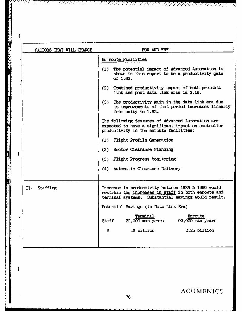
(1) The potential impact of Advanced Autmation isshown in this report to be a productivity gainof 1.62.
(2) Combined productivity impact of both pre-datalink and post data link eras is 2.19.
(3) The productivity gain in the data link era dueto improvemints of that period increases linearlyfran unity to 1.62.
The following features of Advanced Automation areexpected to have a significant impact on controllerproductivity in the enroute facilities:
(1) Flight Profile Generation
(2) Sector Clearance Planning
(3) Flight Progress Monitoring
(4) Autatic Clearance Delivery
II. Staffing Increase in productivity between 1985 & 1990 wouldrestrain the increases in staff in both enroute andterminal systems. Substantial savings would result.
Potential Savings (in Data Link Era):
Terminal EnrouteStaff 22,000 man years 02,000 man years
$ .5 billion 2.25 billion
ACUMENIC(76

.I~~ . .+ .. . . . . ..
FACTORS THAT WILL qAME HOW AND IY
III. Workload Workload would be reduced with the aid of autoimationwhich may result in a productivity gain.
IV. Average Number of One means to achieve enroute ATC productivity gains isControllers per Sector to reduce the average number of controllers per sector.
This can be accamplished by:
(1) reducing support workload;
(2) revising control team organization; and
(3) redesigning control positions
V. Average Instantaneous Another means to achieve enroute ATC productivity gainsAircraft Count per is to increase the average Instantaneous Aircraft CountSector per sector. This can be accaplished by:
(1) increasing "radar" controller capacity; and
(2) increasing capacity utilization efficiency
Contributors to Enroute ATC Productivity
A. 3rd Generation (NAS Stage A)
(1) Automated Flight Data Processing/Forwarding(2) Automated Tracking Displays with Alphanumaerics(3) Autanatic & Manual Display Filtering(4) Surveillance Data lsaicking(5) Simplified Clearance/Coordination Procedures(6) Centralized Flow Control
B. Upgraded 3rd Phase I
(1) Flight Plan Error Correction by Source(2) Autcratic Clearance Coordination(3) Conflict-Free Clearances, including 2_D/3D RNAV(4) Track Conflict Detection & Resolution Aids(5) More Flexible Allocation of Local Control
Capacity4 (6) Man-Machine Interface Improvements (Device
Software)(7) Modifications to Three-a&n Sector Design
(to permit reduced manning under light loads)
*4 ACUMENICS77
FACTORS THAT VLL CHANGE HOW AND ;WHY
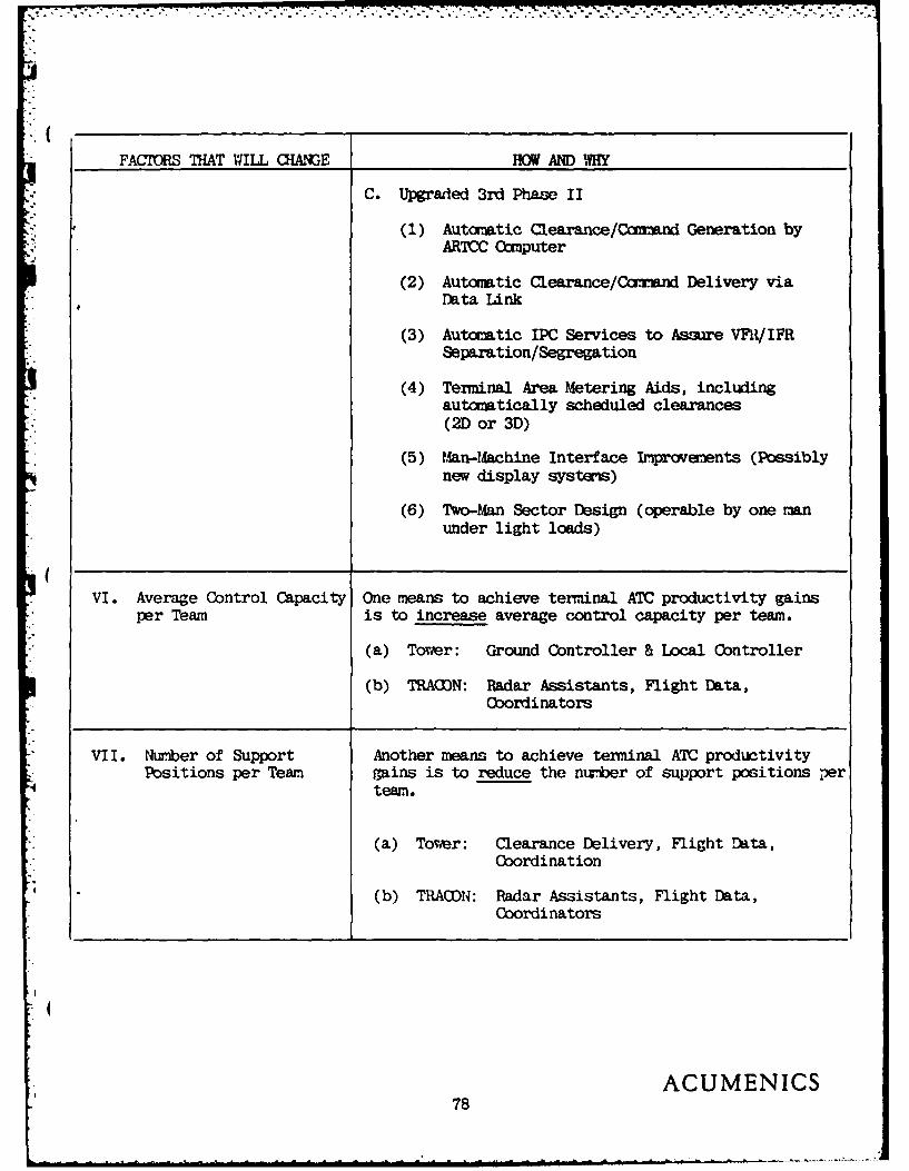
C. Upgraded 3rd Phase II
(1) Automatic Clearance/Caaru Generation byARTCC Computer
(2) Autoomtic Clearance/Cmmand Delivery viaData Link
(3) Automatic IPC Services to Assure VFH/IFRSeparation/Segregation
(4) Terminal Area Metering Aids, includingautomatically scheduled clearances(2D or 3D)
(5) an-achine Interface Improvements (Possiblynew display systems)
(6) Two-Man Sector Design (operable by one manunder light loads)
VI. Average Control Capacity One means to achieve terminal ATC productivity gainsper Team is to increase average control capacity per team.
(a) Torwer: Ground Controller & Local Controller
(b) TRAWN: Radar Assistants, Flight Data,Coordinators
VII. Number of Support Another means to achieve terminal ATC productivityPositions per Team gains is to reduce the nurber of support positions per
team.
(a) Tower: Clearance Delivery, Flight Data,Coordination
(b) TRAODN: Radar Assistants, Flight Data,Coordinators
ACUMENICS78

-I
FACTORS THAT WILL (1A1GE HOW AND WHY
Contributors to Terminal ATC Productivity
A. 3rd Generation (ARTS III, II):(1) Autarted Flight Data Processing/Forwarding
(by NAS Stage A)
(2) Automated Tracking Displays with Alphanumerics
(3) Autaatic & Manual Display Filtering
(4) Simplified Clearance/Coordination Procedures
(5) Arrival Metering & Spacing AutmationB. Upgraded 3rd, Phase I:
(1) Improved Metering & Spacing Automation
(2) Autmatic Clearance Coordination
(3) Conflict-Free Clearances, including 2D/3D RNAV
(4) Track Conflict Detection & Resolution Aids
(5) Man-f-achine Interface Improvements (Device
Software)
C. qpgraded 3rd, Phase II:
(3.) Automatic Clearance/Ccrrand Generation
(2) Autattic Clearance/Caniand Delivery via4 Data Link
(3) Autoaited IPC Services to Assure VRF/IFRSeparation/Segregation
(4) Terminal Area Metering Aids, including auto-matically scheduled (2D or 3D)
(5) Automated Final Approach Monitoring onClose-Spaced Parallel Runways
(6) All-weather Ground Guidance & Control
ACUMENICS79

FACTORS THAT WILL MANGE HOW AND WHY
VIII. Delivery of Flight One means to achieve productivity in the delivery ofServices flight services is to automte the delivery of flight
services. This can be accomplished by:
(1) Autoation aids to FSS specialists; and
(2) Pilot self-service autmation
IM. Nurxber of Flight Another means to achieve productivity in the deliveryService Stations of flight services is to reduce the nmter of Flight
Service Stations required. This can be accomplishedby:
(1) FAA's reconfiguration plan; and
(2) Centralization of services automation
Contributors to Flight Service Station Productivity
(1) The forecast number of flight plans to be handled;
(2) The nuner of individual pilot briefings to begiven.
Approaches to Achieve FSS Productivity Gains
(1) The pilot is encouraged to file his IFR orDVFR flight plan directly with the automatedATC system, thereby eliminating manual handlingof individual flight plans by FSS specialists.
(2) The pilot is encouraged to serve himself inobtaining pre-flight weather and system statusbriefings, rather than depending upon personalizeservice by the F3S specialist.
(3) Where personal briefing services are offered,autonated aids are provided to the FSS specialistwhich significantly reduce the workload associatelwith these services.
ACUMENICS80

S FAMORS THAT WILL qAGE HOW AND MY
(4) Search and rescue services are provided bya more cost-effective method than thefailure of the pilot to cancel his activatedVFR flight plan.
(5) If VFR flight plans are needed, they canbe filed activated, and cancelled directlyby the pilot and/or the FSS specialistwith an automated systen. Entries wuldbe automatically forwarded and booked atone or more centralized locations.
, X. Policy Review; Program Implementation of new ATC systems will require and-4 Planning; Resource induce changes in the processes by which the FAA
Allocation; ,magemnt functions. Operational impacts would be felt inof ATC Services; and these areas.Regulatory Responsibili-
( ties
XI. Comunications; Qhanges in these areas will be caused by technologicalSwveillance Navigation developrents.Procedures; SeparationStandards; AirspaceSectorization; SectorCbntrol Equipment;S-ctor ManningStrategies; and AirspaceTraffic Flow Regulations
ACUMENICS81

FACTORS THAT WILL OIAE HOW AND IHY
XII. Humn Factors These huan factors decribe pertinent performanceA. Job Satisfaction & capabilities of hum~ns.
Ibtivation(1) Achievaeent -
work alignment
(2) Recognition
(3) Responsibility
(4) Control Autho-rity
(5) Utilization ofperceivedskills
(6) Challenge -discretionaryflexibility
(7) PerformanceFeedback
(8) Interest
B. ?,.n-Machine Inter-face(1) Vigilance
(2) Stress
(3) Intricacy
(4) Restrictiveness
(5) Rigidity
(6) Decision/IMaking
C. Failure-MadeOperations(1) Failure Recog-
nition
(2) Failure Re-4covery
(3) Failure Opera-tions
ACUMENICS82

7-7.
V. THE CONCEPT OF PRODUCT IN THE AIRSPACE SYSTEM
The national airspace system can be viewed as a competitive
market within which users buy goods from providers of service.
The users of the system include air carriers, commuters, air taxis
and general aviation. Service providers are the constituent elements
of the federal aviation agency, air traffic control and flight
standards.
The providers of service are producing allowed levels of
activity either in terminal or enroute facilities. Measures of
* such activity include operations, aircraft handled, and aircraft
contacted. The users of the system procure "allowed activity" to
provide for "user produced activity." As such, the levels of activity
* provided by the FAA and consumed by the user are numerically con-
gruent. Thus, for the purpose of this analysis, allowable and user
producedl operations are equivalent.
If one examines the FAA allowable operations, it is seen that
given levels of capital and labor provide a specific range of
operation. Capital in this instance includes the technology
required to provide an a priori specified level of service. In
particular, capital is the technology measured in money terms that
allows the functions defined in the orevious section to be performed
ACUMENICS83

with established proficiency. Labor refers to the number of people
"- required to operate the technology to obtain specific levels of
. product.
Similar for the user side, a given number of aircraft
combined with the set of pilots results in the performance of a
certain level of operations. Labor for the user side is defined by
.. the number and composition of pilots. User capital includes the
:* number and composition of aircraft. Thus for both the system user
and provider of service the relationship can be specified as
Operations - f(LABOR, CAPITAL).
The above specification is similar to that of an industrial production
function in which,
Q - f(LABOR, CAPITAL)
where Q is the product of the industry. The production function
relates the level and composition of production facto:s to
product or service. As such, the production function considers the
* state of technology, or the relative substitution of capital for
4 labor or labor for capital. If the products of two industries are
the same then the production functions of each can be compared for
the same level of product. That is, if industry one has a production
4i function QI - f(Ll,Cl), and industry two has a production function
Q2 = g(L2 ,C2 ) and Q, - Q2 then, f(Ll,Cl) = g(L2 ,C2 ).
ACUMENICS84

The proceeding formulation provides a basis to determine the
* L effects of shifts in productivity factors in one industry on the
quantity of labor or capital in the second industry.
In the context of the present study, shifts in the level or
composition of capital and labor for users will require changes in
the FAA capital and labor to provide the services, or vice versa.
New technology will alter the man-machine relationship in the
performance of functions. However, the change in functiontb will
ultimately affect the levels of capital and labor necessary to
provide a specified level of service. Thus, the production functia
construct may be used to estimate the impact of technological
change on systems users and the providers of service.
The industries of concern are not homogeneous. Rather both the
agency and industry can be desegregated into smaller components.
The agency can be considered to be composed of three industries
that have distinct production functions:
1) terminal areas
2) en route centers, and
3) flight service stations.
4 Each of the above induutry segments has distinct measures of produc
Terminal area product is measured in terns of annual aircraft
operations. Aircraft handled is the measure of en route center
product. Flight service station activity is measured as contacts.
ACUMENICS85

If the notion of product is an acceptable hypothesis for the
airspace constraint, then the effects of new technology can be
measured using the production function construct. The construct
allows one to estimate the relationships among industry product and
the factors of production. Estimates of the present production
function coefficients can be obtained from existing agency data.
The production function coefficients can be modified based on the
estimated change in the efficiency of the technology. The new
technology production function coefficient can then be employed to
estimate the shifts in labor or capital attendant to the new
technology.
ACUMEN ICS

VI. PRODUCTION FUNCTIONS
* The previous section discussed the notion of product and the factors
of production in the airspace system. The production function
construct is used in succeeding sections to estimate the change in
agency labor owing to new technology. This section of the text
will discuss the major production functions. The application of
production functions will be described in the next section.
Since the Cobb-Douglas production function has proved so
useful to the analysis employed in this study, this section pro-
[ vides a non-technical discussion of some of the important concepts
relating to production functions, especially in regard to the
measurement of technological change. Many of these concepts can
quickly involve complicated mathematical expressions that, in a
* technical treatise, would require strict mathematical definition,
derivation and proof. However, this is not a technical economics
* paper and in the discussion below the derivations, proofs, and
even some of the more cumbersome formulas themselves will not be
* fully developed.2 Instead, the general notion of the production
1)For further information, the reader is referred to the follow-ing texts, particularly the first two, Brown, Murray, On the Theoryand Measurement of Technological Change. Massachusetts: TheUniversity Press, 1963; Chiang, Alpha C., Fundamental Methodsof M.athematical Economics (2nd ed.). New York: McGraw Hill, 1974.(Especially pages 186-7 and 404-422).; Lave, Lester B., TechnologicalChange: Its Conception and Measurement. New Jersey: Prentice-Hall,Inc. , 1966, Mansfield, Edwin, The Economics of Technological Change.New York: W. IV. Norton Company, Inc., 1968: Samuelson, Paul A.,.Economics, (9th ed.) New York: McGraw-Hill Book Company, 1973;and Shepard, Ronald W., Theory of Cost and Production Functions.New Jersey: Princeton University Press, 1970.
*~ AC U NI E N I CS87

RD-A125 358 SOCIOECONOMIC IMPACT ASSESSMENT COMMUNICATIONS INDUSTRY 2/2PHASE IV IMPACT'R..(U) ACUMENICS RESEARCH ANDTECHNOLOGY INC BETHESDA RD 21 FEB 81 FRA-APO-8i-il
UNCLASSIFIED DOT-FA78MAI-932 F/G 17/2.1 NL
mommommommoll
onIIImllsIonlllIElllllll lliIIIIEIIIIIIhihI

v I" IIII.II11. 0 .-
".1
mEM'
1.4111 1.6
Iu uI
MICROCOPY RESOLUTION TEST CHARTNATIONAL BUREAU OF STANDARDS-1963-A
7,!

function and how it relates to technological change will be
discussed first. Next, the Cobb-Douglas production function will
be explained in as non-technical a manner as possible, and its
choice for this study explained. Because the Cobb-Douglas formu-
lation is a special case of the constant elasticity of substitution
(CES) production function, that function will then be briefly
defined and discussed. A brief summary will conclude this section.
G:eneral Notion of the Production Function
The production function concept was developed to deal with the
relationship between inputs and outputs, specifically, the maximum
output possible for the various possible inputs to a production
process, given the level of technology, The inputs are generally
abstractly discussed as capital (K) and labor (L) inputs. Paul
ASamuelson defines a production function as follows:
The production function is the technicalrelationship telling the maximum amount ofoutput capable of being produced by each andevery set of inputs (or factors of production).It is lefined for a given state of technicalknowledge.3
Note that the function discusses a technical relationship which
does not depend on the prices of the factor inputs. It can be
expressed as a mathematical function,
Q - f (K,L), whereQ - OutputK - CapitalL - Labor
lSanuelson, op. cit., p. 535.
ACUMENICS88
This general representation says that output is a function-of
(depends on) capital and labor inputs. The assumptions behind this
statement are that only the most efficient production possibilities
are considered, thus only the maximum possible outputs are given
for any combinations of labor and capital, and that the technolog-
ical possibilities are taken as fixed for that point in time.
An invention or a new method of production will chance any
given production function. The production function is usually
shown as a set of curves, called isoquants, on a two-dimensional
graph such as the following (Figure 5-a). Each isoquant shows
that many different efficient combinations of the factor inputs
can produce a given output. If capital (K) and labor (L) are
shown on the axes, then each isoquant line such as A represents
one possible amount of output, Q. For example, if A represents
1000 units of output, then the relationship represented in
Figure 1 shows that 1000 units of output can be produced by using
100 units of capital and 20 units of labor in the most efficient
way then known, or by using 75 units of capital and 30 units of
labor in the most efficient way, or by any other indicated possible
combination of capital and labor. However, 1100 units (shown by
isoquant B) cannot be produced except by using more inputs than
possible on line A.
ACUMENICS89

ISOQUANTS ILLUSTRATING PRODUCTION FUNCTIONS
100
K 75 _ _--.
B - 1100 units
A - 1000 units
0 30L
(b) non-neutral technological change
B'- 1100 units
A - 1000 units
L
Figure 5
ACUMENICS90

-'-~~~wi ST Y .... #**M- ;
Thus we see that, in the general abstract case, capital can
* substitute for labor (or vice versa) in various efficient methods
of production. (Of course the production method chosen will depend
on the relative prices of the inputs, but that does not concern
us here). More output requires an increase in inputs, given the
technology.
When a technological change of any sort occurs, such as a
new invention, a new method of production, a new management tech-
nique, etc., the production function will be shifted. Increases
* in output due to the change will now be possible at least for some
factor input combinations. A useful concept in this regard is
(that technological change can be neutral or non-neutral, depending
*on whether the change affects the relationship between the inputs
* or not.
A neutral change neither saves nor uses labor;it is one which produces a variation in theproduction relation, itself, but does not affectthe marginal rate of substitution of labor forcapital. A non-neutral technological changealters the production function and can be eitherlabor-saving (capital-using) or capital-saving(labor-using). If the production function is
* altered such that the marginal product ofcapital rises relative to the marginal productof labor for each combination of capital andlabor, there is said to occur a capital-using(labor-saving) technological change.4
4Brown, op. cit. pages 20-21.
* ACUMENICS

2j;7~
The nature of technological change may be intuitively under-
stood by looking at Figure 5 (a) and (b). In Figure 5a, a neutral
technological change would mean that the output (1100) previously
possible from the various factor combinations shown by isoquant
B can now be produced, say, with the factor combinations indicated
by the old isoquant A. In other words, the same factor inputs now
can produce more output than before, and if more of one factor is
used, less of another is needed; the marginal rate of substitution
"" between capital and labor remains the same.
A non-neutral technological change can be illustrated by
Figure 5b, where before the change, 1100 units of output are
possible from any of the factor combinations shown on isoquant B'.
*. After the technological change, 1100 units are now possible from
the various factor combinations shown on A; however, the marginal
rate of substitution of capital for labor is different on the two
" isoquants, A and B'.
Murray Brown has found the production function to be a useful
* tool in the measurement and analysis of technological change. He
"" develops the concept of 'an abstract technology,' and states,
* "It is relatively easy to define a technological change in terms
of a change in the characteristics of an abstract technology."5
That is, if a production function relationship is shown to change
(5page 12.
ACUMENICS92

over time in certain ways as we shall see below, the changes can
indicate and to some extent quantify the type and effect of the
technological change that is occurring.
The four characteristics of interest in measuring and analyz-
ing technological change are: (1) the efficiency of a technology
(2) the degree of economies of scale that are technologically
determined; (3) the degree of capital intensity of a technology
and (4) the ease with which capital is substituted for labor.6
Brown's definitions, which are useful, follow.7
(1) Efficiency -- This characteristic ... enters onlythe relationship between inputs and outputs; itdoes not affect the relationship of inputs toinputs. For given inputs, and given the othercharacteristics of an abstract technology, theefficiency characteristic determines the outputthat results. If it is large, then output islarge. ... One can think of ... (it) ... as ascale transformation of inputs into output.
(2) Technologically determined economies of scale --For a given proportional increase in all inputs,if output is increased by a larger proportion,the firm enjoys increasing returns (or economiesof scale); if output is increased by the sameproportion, there are constant returns to scale;and if output is increased by a smaller proportion,decreasing returns result (or diseconomies ofscale).8
6Ibid.
7 1bid. pages 13-19.
8 Economies of scale are often further classified as internaleconomies, which depend on the operation of the individual firm,and external economies, which depend on the general developmentof the industry or the economy as a whole.
ACUMENICS93

(3) Capital intensity -- Degrees of capital intensityare reflected in the size of the labor-capitalratios for given relative factor prices.9
p
(4) The ease with which capital is substituted for labor --
The elasticity of substitution *.. ( ) ... tells ushow rapidly diminishing returns set in to one factor
* 4 of production ... (it) ... relates the proportionalchange in the relative factor inputs to a proportionalchange in the marginal rate of substitution betweenlabor and capital ... Intuitively, it can be thoughtof as a measure of the ease of substitution of laborfor capital; it can also be conceived of as a measureof the 'similarity' of factors of production from atechnological point of view.1 0
Changes in the efficiency of technology and changes in econo-
mies of scale may be thought of as producing neutral technological
change. Changes in the capital intensity of a technology and in
( the ease of substitution of capital for labor produce non-neutral
technological change.11
Cobb-Douglas Production Function
The Cobb-Douglas Production Function and the Measurement of
Technological Change:
9Usually capital intensity is thought of as the quantity of* capital relative to the quantity of labor, or the capital-labor
ratio. Brown wishes to emphasize the necessity of eliminatingthe influence of relative factor price in the short run, on thisratio.
1OThe concept of "constant elasticity of substitution," wherebythis measure does not vary over the possible production process,will be important below. The Cobb-Douglas and, of course, theCES production functions both assume a constant elasticity ofsubstitution.
1 1 Ibid. page 21.
ACUMENICS94

-~~ "T"TEl
The generalized expression of a Cobb-Douglas production
function is
QAKO LO 12
where, again, Q -output, K -capital, and L -labor. A, a andB
* are constants to be determined empirically, and depend, of course,
* on the technology. The Cobb-Douglas formulation of the production
function is easily reformulated in logarithmic form:
ln Q l n A + ctln K +- Bin L. One reason for the wide
use of this formulation is that it can then be applied in a
straightforward manner to the available data, using least squares
regression techniques. Again, note that the Cobb-Douglas function
is a special case of the CES production function, which will be
( discussed further below.
Of interest for our purposes is the interpretation of these
parameters A, a , and 8,as indicators of technological change.
Following Brown's schema (pp. 40 ff), the interpretation follows.
12More properly, in..a Cobb-Douglas production function, therestriction that (a + 3. ) is imposed, and the function canalso be written Q = AK L(1-0. This is a "linearly homogeneousproduction function of degree one," which means that if K and Lare increased by p ercent, Q will also increase by exactly ppercent (that is, p percent!). In the more general case, if(a + B-r), a linearly homogeneous production function of degree rwill mean that if K and L are increased by p percent, Q will beincreased by p percent. See Chiang, op. cit. p. 406 ff.
ACUMENICS95
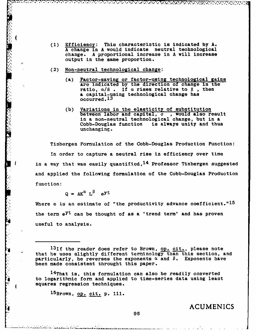
(1) Efficiency: This characteristic is indicated by A.A change in A would indicate neutral technologicalchange. A proportional increase in A will increaseoutput in the same proportion.
(2) Non-neutral technological change:
(a) Factor-saving or factor-using technological gainsare indicated by the direction of change in theratio, a/B If a rises relative to , thena capital-using technological change hasoccurred.13
(b) Variations in the elasticity of substitutionbetween labor and capital, a would also resultin a non-neutral technological change, but in aCobb-Douglas function is always unity and thusunchanging.
Tinbergen Formulation of the Cobb-Douglas Production Function:
In order to capture a neutral rise in efficiency over time
( in a way that was easily quantified,14 Professor Tinbergen suggested
and applied the following formulation of the Cobb-Douglas Production
function:
Q =AKXL0 eYt
Where e is an estimate of "the productivity advance coefficient."'15
the term eyt can be thought of as a 'trend term' and has proven
useful to analysis.
.* 1 3if the reader does refer to Brown, op. cit., please notethat he uses slightly different terminology than this section, andparticularly, he reverses the exponents a and 8. Exponents havebeen made consistent throught this paper.
14 That is, this formulation can also be readily converted* to logarithmic form and applied to time-series data using least, 4 squares regression techniques.
15 Brown, op. cit. p. 111.
96 ACUMENICS
96

CES Production Functions
The generalized form of a constant elasticity of substitution
(CES) production function is
Q - A [ 6K- P + (1-6)L-P]-V/p
* (Where A > 0; 6 > 0; p > -1). While this function assumes the
elasticity of substitution is constant, it is not restricted to
one or any particular value. However, this formulation is,
according to Brown, statistically "relatively unmanageable,"16
and it has not been used in the present study. It has already
been noted that the Cobb-Douglas production function used is a
*. special case of the CES production function, where the elasticity
*% of substitution is constant and unitary.
(Of interest for our purposes is the meaning of the coefficients
in this formulation for understanding and attempting to measure
technological change. Admittedly, the meanings are somewhat flawed
in some cases. Again following Brown and Chiang the following
interpretations are suggested.
(1) Efficiency is again represented by A: it indicatesthe state of technology.
(2) Capital intensity is represented by 6 . 6 has todo with the relative factor shares in the product.
16 1bid. p. 128. For one thing, it is difficult to generalizeto more than two factors of production; also, the statisticalapplication is considerably more cumbersome. The logarithmicform does not yield an expression that can be evaluated by directapplication of least squares regr.ssion techniques. For furtherdiscussion of these and c, her pr- lems, see Brown, esp. Chapter 9.
ACUMENICS97

[-77 I*-
( (3) The degree of returns to scale is represented by v. Itshould be noted that v can change for two reasons, anexpansion in the scale of operations or a technologicalchange that alters the rate of growth; v does not dis-tinguish between the two causes.
(4) The ease of substitution of capital for labor isindicated by p . If the elasticity of substitutionis a , p = -(i-i/ a )17
Summary
Although the abstractions necessary to quantify a production
function necessarily entail some deficiencies in the final formu-
lation, 18 the concept of a production function has proved fruitful
for the analysis and measurement of the economic effects of tech-
nological change. In particular, the Tinbergen version of the
Cobb-Douglas production function has been foand both quantifiable
and useful. This formulation was found to be relevant to the
present study since the data exploration indicated that its use
was appropriate. The Tinbergen-Cobb-Douglas production function
formulation was used throughout.
17Chiang, p. 419, shows that if -1 < p < 0, then a > 1if p = O, then a = 1if 0 < p < -, then a < 1.
18 The reader is referred to the works referenced here, orother intermediate economics texts, for a full discussion of thedeficiencies of the Cobb-Douglas production function. Of course ilis clear that the pre-specification of a unitary elasticity of sub.stitution might be a drawback; however, this specification oftenfits the data well. Other statistical problems, such as colli-nearity, can arise when it is applied to time series data; thesemay be reduced by the use of the trend term in the Tinbergen speci-fication. And finally, any interpretation of the meaning of thecoefficients can be open to discussion, given the present state of
.• knowledge in this field. This section did not attempt to discussmany other interesting aspects of production functions, such astheir use in examining factor shares of income.
ACUMENICSK - 98
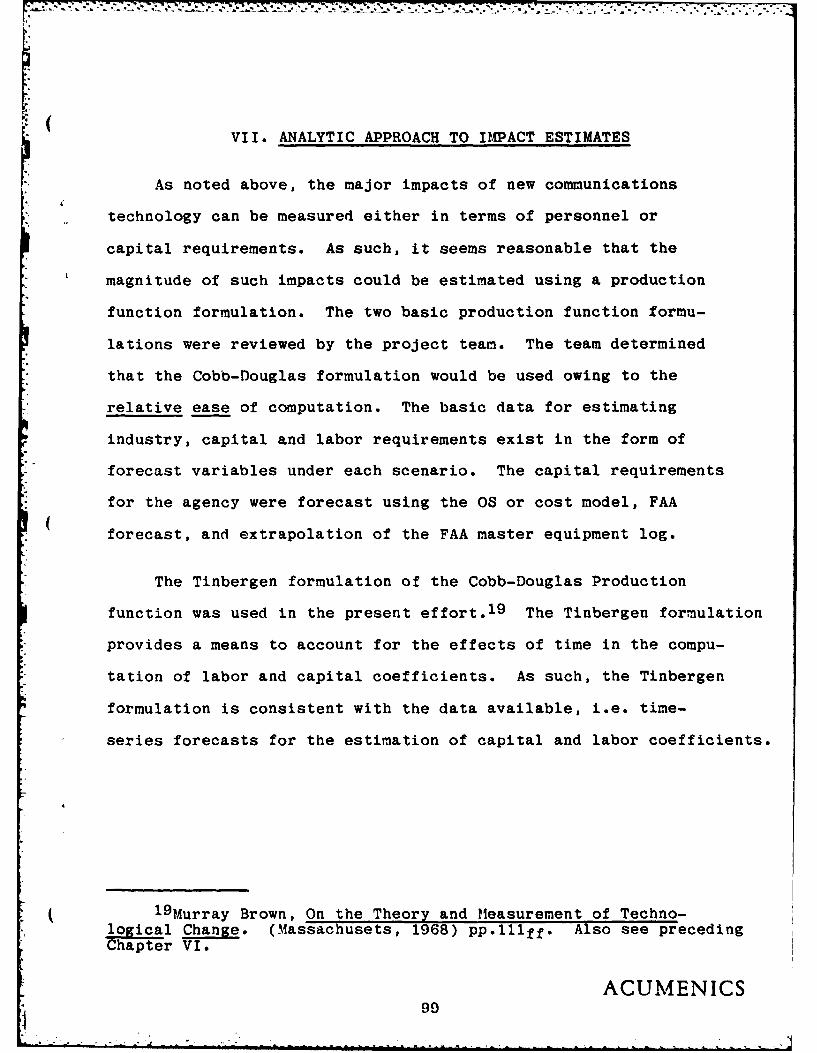
VII. ANALYTIC APPROACH TO IMPACT ESTIMATES
As noted above, the major impacts of new communications
* technology can be measured either in terms of personnel or
capital requirements. As such, it seems reasonable that the
magnitude of such impacts could be estimated using a production
function formulation. The two basic production function formu-
lations were reviewed by the project team. The team determined
that the Cobb-Douglas formulation would be used owing to the
relative ease of computation. The basic data for estimating
industry, capital and labor requirements exist in the form of
forecast variables under each scenario. The capital requirements
for the agency were forecast using the OS or cost model, FAA
forecast, and extrapolation of the FAA master equipment log.
The Tinbergen formulation of the Cobb-Douglas Production
function was used in the present effort.19 The Tinbergen formulation
provides a means to account for the effects of time in the compu-
* tation of labor and capital coefficients. As such, the Tinbergen
formulation is consistent with the data available, i.e. time-
series forecasts for the estimation of capital and labor coefficients.
19Murray Brown, On the Theory and Measurement of Techno-
logical Change. (Massachusets, 1968) pp.11 1ff. Also see precedingChapter VI.
ACUMENICS99

*. . ... .... . .. .. . . _*_ .. . . . ..
* ..
The general Tinbergen model is
Q = AKa L eYt
where
Q= productK = capital
* L = labort = timeA,a , y are empirically determined
* coefficients.
The two major components of the airspace system are terminal
areas and en route airspace. The users of such airspace are
different. That is, terminal areas are used by general aviation,
* airtaxis, commuters, corporate aircraft as well as aircarriers.
En route airspace is used predominately by aircarriers, commuters
- and corporate aircraft. As such, it was determined that separate
production functions would be estimated for en route and terminal
-" airspace. In addition two sets of production functions must be
examined for each portion of airspace: system users and providers
of service. The basic aggregate measure of product in a terminal
area is total operations (TOPS). TOPS are comprised of local
operations (LOPS) and itinerant operations. The user capital in
the terminal area includes the active general aviation fleet,
(GACAP) as well as the aircarrier fleet capital (TACAP). The labor
• "component of the user includes the total pilots active in the
terminal area (TPLT). The generic user production function in the
i
ACUMENICS100

terminal area can be specified as follows:
TOPS - A(TCAP)' (TPLT)a eYt
where TCAP = P(GACAP) + R(TACAP).
and P, R are the relative cost of the capital units. The agency
or services providers generic production function also uses TOPS
as the product. However, capital (CTER? ) is defined as the consumed
value of agency communication facilities in the area. Labor is
defined as the array of government personnel, primarily controllers
(TERM), necessary to manage TOPS. The generic agency production
function is
TOPS = A (CTERM)a (TERM) e Y t.
The use of en route airspace is dominated by aircarrier opera-
tions. As such the capital and labor attendant to such use is
emoodied in the aircarrier fleet and the transport pilots (TRANP).
The measure of product in en route airspace is aircraft handled
(AIRHAND). The estimate of en route product or workload is based
on the number of IFR Departures (TIFRDEP) and overs (OVERS). As
such the generic production function for en route space users is:
AIRHAND = A(TACAP) a (TRANP)s eYt.
where TRANP = transport pilots and TACAP = aircarriers fleet
capital.
The agency and user production function employ the same measure
of product, i.e., AIRHAND. The agency measure of capital is the
consumed quantity of technology necessary to service AIRHAND (CCENT).
The labor component of the production function is the number of agenc
ACUMENICS101

(2
personnel necessary to perform center(en route facilities)functions
(CENT). The generic agency en route production function is:
AIRHAND = A(CCENT)a (CENT) eYt
It should be noted that user and agency production functions are
estimated for each scenario. The effects of new technology are
considered by estimating production functions constructed for
the following time periods:
1981 - 1990
9.
1991 - 2000
2001 - 2010
2011 - 2020
( The actual estimates were prepared using a log linear form
of the production function, i.e.,
ln(TOPS) = lnA + a ln(CTERM) + B ln(TERIM) + yt.
During the curve fitting exercise certain restrictions were imposed:
.a+ 8= 1,
a > 0,
S > 0,
The log linear user production function and appropriate
statistics for each scenario are shown in Tables 12 - 14.
It has been assumed in this analysis that the largest
*- individual unit effects of technology will accrue to the agency.
In addition, new technology adopted by users will be conpatible
( with agency investments. That is, users will not invest in new
ACUMENICS102

?AKEI 12
in cmm ina ~ in (mw). Bin CMu) * t
YEAS M121W 7CAP I=W
2991 - 200 1.2185 Am1 JIM2 AMO
2001 - 2010 1.407 .2744 .7396 -.0658
2011 - 22M 2.008D -I=6 .7634 -.90m
In (*AIW)MM In A. aLa (TWOP) $ In (TRAW) 4-y
199 - Mw0 6.2161 .0111 AMN -. OM6
2001 - 2010 4.6011 .1254 .75-03
2011 - 220. .6652 .4070w
U ACUMENICS103

*P -
USER PfM CN FERCTI(K COF CIEMT
In (T S) - in A + C In (TCAW) + 0 la C1PLT) + 7t
1991 - 200 1.4506 .2670 .732D .0001
2001 - 22010 1.3m50 .2544 .7455 .00005
2011 - 0 1.6m o2484 .7535 .00003
in (AMMD) -In A. +*In (TAAP) 0 BIn (TflW) + yt
YERSM !mW TICAPmu t
1991 - 20W -4.1450 .7357 .2ft2 .0013
2001 - 2010 -3.4733 .rum .3128 .00006
2011 - 2020 -3.0,1 .580 .344044 .0000
104 ACUMENICS
1

wT- T-T -. 4...* _
TAE 14
InAR -M In A 4 M (TCIP) .In CWI.) .t
1991 - 2m1.117 .2879 JIM3 4m0
2001 - 2010 1.3508 =244 .7255
2011 - 20 1.89M8 .2305 .76M4 4m0
In (AURHAN) -In A +ag In (ThCAP) +8 in (IRmP) + yt
(EM { IWIHZPr TP.CAPRM t
1091 - 2=0 1.69M0 .31945 .68055 -. 0040
27001 - 2010 2.4275 .27002 .7209 -. 0001
2011 - '2020 4.2090 .1455 .8544 -. 0090
ACUMENICS105

technology that cannot be employed in the airspace system.
As such, the characteristics of the technology forcasted in
previous sections of this effort will weigh most heavily in
the coefficients of the agency production functions. The one
technology characteristic that is likely to alter the division of
labor in function performance is speed in data processing. That
is, system speed will allow greater substitution of capital for
labor in many of the functions specified in preceding sections
of this work. The agency production functions will be specified
based upon the technology forecast parameters, rather than
forecasts of activity measures. In particular, production function
estimates were determined for one scenario, i.e., stagflation.
It was assumed that the continued presence of existing agency
technology beyond 1990 would represent conditions under the
stagflation scenario. As such, agency production functions
were estimated for the time period 1971-1981. As indicated
before the functions of interest are
AIRHAND = A (CCENT)a (CENTP eyt
TOPS = A (CCTERH) a (TERM) e eyt
ACUMENICS106

(
*The estimates were based on the log linear forn of the relationship.
ln(AIRHAND) - lnA + a ln(CCENT) +0 ln(CENT) + yt
ln(TOPS) - lnA + aln(CTERM) + Bln(TEIR) + yt.
As noted above, the coefficients for the agency production
function were altered based upon the relative increase in speed
of VLSI data processing equipment projected in the technology
forecast. The basic data processed are shown in Table 15.
If stagflation is taken as the base case, i.e., stagflation - 1.00
then equivalent values for balanced growth and rapid growth
are 1.05 and 1.15, respectively. That is, the net efficiency under
( balanced growth will be 5% greater than under stagflation. Under
rapid growth the speed will be 15% greater than under stagflation.
As such, one would expect similar differences in the production
function capital coefficients for the balanced and rapid growth
scenario when compared to the stagflation scheme. The agency
log linear production function coefficients for each scenario are
presented in Table 16. The application of the production functions
will be described in the next section.
ACUMENICS107

TABLE 15
VLBI DATA PROCISS CHARA ISTICS
SPE (MIPS)
YEARS 3A RM G 8L?,S1ATX0 RAPID O
1960 3.1 3.1 3.1
1365 7.8 6.9 0.8
1990 15.6 13.2 2D.90
200 41.7 37.78 47.22
.. I YEARS WAA1D QU'1I SI ATION RAPID GR1~H
10 1.0 1.0 1.0
1M65 1.13 1.0 1.42
190 1.18 1.00 1.59
200 1.10 1.00 1.24
Aveg 1.10 1.00 1.31
-~ .'%t RelativeW. Efficiency 0.06 0.00 .15
ACUMENICS108
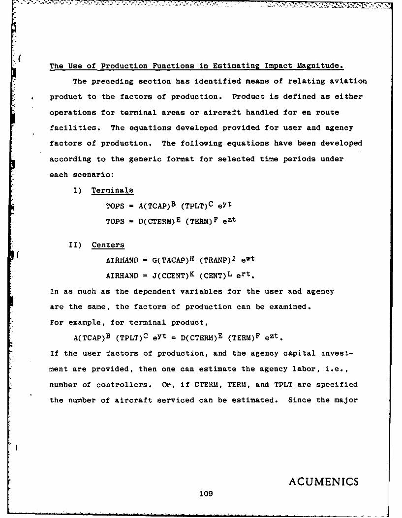
i77
The Use of Production Functions in Estimating Impact Magnitude.
The preceding section has identified means of relating aviation
product to the factors of production. Product is defined as either
*i operations for terminal areas or aircraft handled for en route
facilities. The equations developed provided for user and agency
factors of production. The following equations have been developed
according to the generic format for selected time periods under
each scenario:
I) Terminals
TOPS - A(TCAP)B (TPLT)C eYt
TOPS - D(CTERM)E (TERM)F ezt
II) Centers
AIRHAND = G(TACAP)H (TRANP)I ewt
AIRHAND = J(CCENT)K (CENT)L ert.
In as much as the dependent variables for the user and agency
are the same, the factors of production can be examined.
For example, for terminal product,
A(TCAP)B (TPLT)C eYt = D(CTERM)E (TERMA)F ezt.
If the user factors of production, and the agency capital invest-
ment are provided, then one can estimate the agency labor, i.e.,
number of controllers. Or, if CTEWA, TERM, and TPLT are specified
the number of aircraft serviced can be estimated. Since the major
ACUMENICS109

".
'"(
TABLE 16
AGECY PRCIDI rlN FU4C'I0IK OW ICIE1TS TERINAL: 1991-2020
U-
In (TO'S) -in A eIin ( +li 8 in (TERMA)
SCEAIO INrERCEr in (CEW in (TEWO
STAGI ATION 5.836028 .188336 .338924
':'"BAI.ANCED
5.838928 .195053 .329607
RAPID5.83698 .2070 .320270
i(
In (AiRAND) in A + (I In (CCET) + in (c€lr)
S:EARIO IzrmECr In (C::T) In (OCl)
ii"rL.'rIGN 2.109721 .440310 .31KJ*2
BALANCEn2.109721 .462326 .2D7176
RAPID2.100721 .484341 .275161
74
* ACUMENICS110

individual impact will accrue to the agency, the relationships
will be used to estimate the impact of
1) varying capital intensity on the number of controllers
2) varying number of controllers on capital intensity.
ACUMENICS
o11

r..
VIII. SPECIFIC EFFECTS
As noted above, the primary effect of communication technology
will be to change the division of labor between man and machine.
As such, the functions performed by man and machine will be
automated further.
It seems reasonable that the technology adopted by the agency
will influence that used by the industry. That is, industry will
use technology compatible with that adopted by the agency. Such
industry use will be accomplished voluntarily and/or by regulation.
Therefore, the primary impacts of concern here are those occurring
to the agency.
The initial result of technological use is to shift respon-
sibility in the performance of funtions. As the machine-man
division of labor changes so do the relative composition of the
factors of production. Therefore, the net and measurable effects
of technological change are:
o changes in the level and nature of agency capital invest-ment;
o changes in the magnitude and composition of the agencywork force
The present effort will examine the agency impacts for the three
principle components of the airspace system:
1) terminal areas,
2) en route facilities, and
3) flight service stations.
ACUMENICS112

77.
A change in the level of capital investment will be estimated
based upon the system concept, innovation lag factor, and nature
of the technology developed in the technology forecasts. Estimates
were prepared based upon an examination of the agency's current
agency and historic capital stock, current agency estimates, and
* other relevant published documents. Capital requirements by year
were developed for each scenario.
The agency staff impacts were estimated using production
- function constructs. Current and historic capital and labor
coefficients were estimated. The coefficients were modified based
* upon a change in the relative efficiency of technology across
( scenarios. Staff estimates were computed based upon the adjusted
production function coefficients. The results are reported in
* terms of staff magnitude for each scenario, as well as for cross
scenario conditions. That is, staff levels have been developed
for the following generic cases:
scenario technology - scenario capital =scenario activityscenario technology = scenario capital ~'scenario activity
- For example, the effects on staff level are estimated where balanced
* growth activity occurs in conjunction with an investment in rapid
growth activity. In addition, staff productivity measures were
calculated to place the impact measurement in the appropriate
- context. The productivity measures estimates vary with the component
of the airspace system considered:
ACUMENICS113

System Component Productivity Measure
terminal areas .... . . total annual operationsper terminal staff
en route . . . . . . . . . . . . total annual aircrafthandles per center employee
FSS .............. total flight servicesper FSS employee.
An increase or decrease in productivity is measured by changes
in the activity per employee measures. The activity per employee
measures indicate also the impact of the technology on operations
efficiency.
Estimates of the communications load are presented also.
Communications load estimates consider the magnitude and com-
position of messages for the terminal and center components of
the airspace system.
4 -
ACUMENICS114

IX. CAPITAL COSTS
Introduction
The effects of new communications technology on the air traffic
control system have been estimated by assuming that the products
of the system (aviation operations) are related to the capital and
labor employed according to the following relationship:
Q =AKa L
where Y represents units of operation, K and L represent capital
consumed and labor hours employed respectively, A is a coefficient
of efficiency and a and 8 indicate the elasticity of output with
*respect to capital and labor. The form of the relationship is
that of a Cobb Douglas production function.2 0
The first requirement for using the function in the present
context is to estimate the values of its coefficients. Historical
data for the period 1970-1980 were available from the FAA on avi-
*ation's operations and labor hours. Estimates of capital consumption
during the same decade have been prepared in order to calculate
values for the coefficients.
The effects of changes in communications technology can be re-
*presented as improvements in both the amount of capital employed
2 0 Meghnad Desai, Applied Econometrics (New York: McGraw-Hill BookCompany, 1976), pp. 111-112. See also Chapter VI.
ACUMENICS115
_ - . --

... .. ..........
to support air traffic control functions and the efficiency with
which capital is used. Improvements will be reflected in reduced
manpower requirements for the air traffic control system. The
plan for the present forecast and assessment effort is therefore
~. to project aviation operations and air traffic control capital in-
vestment over the forecast period (1980-2020), and then to derive
future manpower requirements using a Cobb-Douglas production func-
tion. Aviation operations have been projected by the FAA to 1990,
and these estimates have been extrapolated to 2020 for purposes of
the present report. It has been necessary to construct projections
of capital consumption as well.
( This section of the report describes the sources of data and
* assumptions used to estimate capital consumption during the historical
* period (1970-1980) and the forecast period (1980-2020). The histor-
ical data is described first. Projections for the forecast period
* are then presented for each of three economic scenarios, identified
* as stagflation, balanced growth, and rapid growth.
Historical ATC Capital Growth (1970-1980)
Since the focus of this technology forecast and assessment
is communications, capital consumption has been estimated for
communications related facilities and equipment (F&E) in the air
traffic control systeri. The categories of F&E that have been
ACUMENICS116

identified with communication functions are adopted from a recent
series of reports on the subject prepared f or the FAA.21 All air
traffic control (ATC) facilities and equipment have been assigned
to one of the following three areas: terminals, en route centers
and flight service stations. The rate of capital consumption for
the period 1970 to 1980 has been calculated from historical data
on replacement costs and an assumed aggregate useful life of 14
years. The total for all communications related facilities and
equipment increased from $125.7 million in 1970 to $275.1 million
in 1980. Details for terminals, en route centers and flight
service stations are shown in Table 17.
( The sources of information for historical F&E costs are sum-
marized in Tables 18, 19, and 20. Terminal facilities and equipment
(Table 18) are classified according to function as control (e.g. air
traffic control towers), communications (e.g. remote transmitter/
receiver facilities), surveillance (e.g. airport surveillance
radars), and navigation (e.g. inner, middle and outer radio marker
beacons). Facilities and equipment at en route centers (Table 19)
are assigned to similar categories under the headings: centers
(e.g. air route traffic control centers), communications (e.g.
remote center air/ground communications facilities), surveillance
21Wq. M. Kolb and I. Gershkoff, "FAA Communications Cost Model- ( User's Guide (Revised)," prepared by ARINO Research Corporation
for the Office of Aviation Systems Plans, (April 1980).
4 ACUMENICS117

.( TABLE 17
ANNUAL CAPITAL CONSUMPTIONAIR TRAFFIC CONTROL, SELECTED FACILITIES AND EQUIPMENT
(99 1970 - 1980(1979 DOLLARS IN THOUSANDS)
En Route. Year Terminals Facilities FSS Total
1970 36,747 83,968 4,948 125,663
1971 41,524 89,585 5,512 136.,621
1972 46,923 95,577 6,139 148,639
" 1973 53,024 101,970 6,838 161,832
1974 59,918 108,791 7,616 176,325
1975 67,708 116,068 8,483 192,259
" 1976 72,806 121,340 11,121 205,267
( 1977 78,289 126,852 14,580 219,721
" 1978 84,184 132,615 19,114 235,913
" 1979 90,523 138,639 25,058 254,220
1980 97,339 144,937 32,851 275,127
Source: Tables 2, 3 and 4.
ACUMENICS118

Table 18
Air Tmffic CmU401 Selected Facilities and 4uipmentTzmminal Replaceut Cato
..oiW-t unit Costs inventory Unit Costs Inetr unit Com Inenor
..C 411.000 331 t11.000 400 42,000 49TRAD/TRACAB 61,00 84 011.000 75 881.000 78I8M 96.000 20 94,000 302 142,000 303RB0010 193 100,000 300 151,000 101ARTS W4,000 2 M56,00 81 96.000 03( ST 687.000 47 MY7,00 2 1,03,000 5CTRAC 2,.20,000 2 2,000.000 0
87,000 =,200 737 132,000 791I v 50,00 4 50,000 4 79,000 4
.20,000 72 2D.000 16 30.000 211C= 46,Oo 2 48.300 19 70.000 13UL. 100.000 6 100,000 8 151,000 5
0 S60,000 123 64.300 171 975,000 181PAR 7M6.000 a 786,000 9 1.189,000 8
XAVIGATON
FJ 12.00 48 12,000 42 18.000 36H 46,000 170 46,000 0213 9,000 20711' 35,000 47 85,000 13 130,000 9L.0 123,000 12300 586 186,000 67
35,000 39 74,100 55 120000 59stl 12,000 2D2 12,000 34 18,000 57701 12,000 306 12.000 542 18,000 12LI/L t 18,500 236 18.500 386 3,000 378U1 7,400 18 7.400 50 11,000 05
(1) vei-t avmse of .s I (@ 250,000) and ARTS I ( s1,078, ).
-((2) rey Units assigned t T Pm 1972. Aviation Mot? Allocation study.
(3) N'ineteen Units Usignef tn an -Pita ft-ilttem -Mr 10 A-1ation ^-"?Vilocation StUM7.
(4) All 123 AS's ar. o the types AMI 2-7 having a weighted awnrg costOf o600,000.
(5) Includes all H and MU1 facilities, thoe asMined to both en route andFS facilities. The 1972 Aviation Cost Allocation Study assigned themas follows:
Te omals R 101 1 546,000 111 0 0 585,000
En Route Facilities H N8 0 46,000 MI1 47 0 885,000
*,"SS 1 11 4 06,000 Mi 0 0 585,000
(,1) Includes RM's at FSS facilities. Cost is a weighted avwuge cost per1972 Aviation Cto t Allocation Study: 1M 103 units (e $40,000);
(7) Includes OLT's at FS3 facilities. Cot is a weighted average ocat per1972 Aviation Cost Allocation Study: M55 4 units (0 $101,000);Terminals 24 unitr (0 336,000).
Sources: C. Paul F. Dienemnn, et. al., "Aviation Cost AllocationStudy: FAA Airport and A.rwy System cost Elmsnt."Prepared for the Office of Policy Review - FAA (Feb. 1972).Table 2: "rport System Costs".Table 3: "Teritnal Central Systems Costs"."able 4: "En Route Central Syxtau C sts".Table 5: "Fliiht Service Syuti Costs".Table 0: "Support System Costs".
S.A. Klein, S.C. .o.vioff &Mv E.I. Beok, "FAA O7mmmicationeCost b el and Projections 1075-20W0".Prepared for the Office of Aviation Policy - FAA - byCnputer Sciences Crporation (DOc. 1975).Table 0-7: "F & E Average fteplaent Costs Wy
FacLlity Type".Table 3-2: "Matribution of Facilities by Class
by ARTM-
V.1.I. Kolb and I. rershkof:, "FAA Qwunications 00st '-le1Use's =A.Is (Revised)". IlrepAred by ARM~ R ACU M N r0orporation for tie Office Of %viation Systan plane C M N C(April, 1060).Appendix A: "Facilities and 'iquil~mnt Cost Allocati n".Appendix D: "Facility C3tetry ?becriptUins".
119

V
Table 19
Air Traffic Control, Sleceto Facilities and EquipomntEn oute Center Replaern 3Omt
Facilities 1972 1972 I= *MEquipmnt Unit Costs Inventor Unit Costs Invetry Unit Csts Ja_ tc
ARTCC 13,618,000 25 13,818,000 5 20,5W9,000 23CrRB 1,100,000 24 1,100,000 24 1,644,000 500C - 7,500,000 1 11,345,000 20
- . DPS (EVS '72) 1,100,000 0 1,100,000 5 40,372,000 1
03ZLNICATICNS
RCAG 161,000 458 161,000 525 244,000 550LVM 33,000 a 33,000 10 50,000 8tL.T 33,000 106 33,000 108 50,000 84R(CPO 405,000 2 405,000 3 613,000 3Cr 50,000 1 50,000 1 76,000 1
2FDEP 20,000 19 20,000 19 30,000 19
SURVEILLANCE
ARSR 2,180,000 91 2,180,000 108 3,298,000 102MILR 110,000 495 110,000 521 166,000 518MILT 108,000 215 108,000 247 163,000 213BVEC - 80,000 98 80,000 204CD- 133,000 37 201,000 107
NAVIGATION AIDS
C ( (VAMR R TP) 248,000 885 248,000 94 374,000 93110 8,000 73 8,000 85 12,000 66
SELA 93,000 13 93,000 is - -
'L 64,000 13 64,000 --
Sources: C. Paul F. Dienemann, et. al., "Aviation Cost AllocationStudy: FAA Airport and Airway System Cost Element."Prepared for the Office of Policy Review - FAA (Feb. 1972).Table 2: "Airport Systems Costs."Table 3: "Tenrinal Central Systemw Costs."Table 4: "En Route Central Systems Costs."Table 5: "Flight Service Systas Costs."Table 6: "Support System Costs".
S.A. Klein, S.C. Novikoff and E.M. Bosek, "FAA CommunicationsCost Model and Projections 1975-2000." Prepared for theOffice of Aviation POlicy - FAA - by Cumputer SciencesCorporation (tlec. 1975).Table 3-7: "F & E Average Replacement Costs by
Facility Type."Table B-2: "Distribution of Facilities by Class
by ARTCC -
W.M. Kolb and I. Gershkoff, "FAA Comunications Cost 1*,delUser's Guide (Revised)." Prepared by ARINC ResearchCorporation for the Office of Aviation System Plans(April, 1980).Appendix A: "Facilities wid Equipment Cost Allocations."Appendix D: "Facility Category Descriptions."
ACUMENICS120
|..

• " ",~ " -- . - "---t.. t- --------------- - '-" ------ --- _- _._ . o ': _! _. i - o-',:. ' -
Table 20
Air Trffic ontrol, Selected FaCiliti and qiuEpntFlight Service Station Rplacsinent Cbats
Facilities 1972 1972 ) 1975 1978 1M
* Euioment Unit COM Inetr unit COint Invetor unit Coats Inventory
'STrATIOt
753 77,000 334 76,300IFSS 1,590,000 8 1,560,000 116,000
7FSR - 795,000 2,405.000IWST M150000 1,203,000CRES - l 2,250,000 794,000IATSC 2,250,000 2 - 41,000AM 2,700,000 1 4,992,000 3,403,000I.SC 4,992,000 1 20,000 -(, 7,551,000
30,000O7X1UICATION3
12a) 158,000 24 158.000 35 230,000 904LRGD 11,700 484 11,700 587 18,000 581C'C* 28,000 14 38,000 17 42,000 18MF 22,000 6 35,900 23D 54,000 205LDA - - 100,000 3 17,000 10SF- --7,000 77 41,000 128SSO - 50,000 4 76,000 3
Sources: C. Paul F. Dienemann, et. al., "Aviation Cost Allocation* (Study: FAA Airport and Airway System Cost Element."
Prepared for the Office of Policy Review - FAA (Feb. 1972).Table 2: "Airport Systes Costs."Table 3: "Terminal Central Systems Coats."Table 4: "En Route Central Systems Costs."Table 5: "Flight Service Systems Costs."
S.A. Klein, S.C. Novikoff and E.M. Bosek. "FAA CmmmicaticonsCbst Mdodel and PrTjections 1975-2000." Prepared for theOffice of Aviation Policy - FAA - by Cmnputer Sciences(brporation (Dec. 1975).Table B-7: "F & E Average Replacement C ts by
Facility Type."Table 8-2: "Distribution of Facilities by Class
by ARTCC -
W.M. Kolb and I. Gershkoff, "FAA Camunications Cost MoadelUser's Guide (Revised)." Prepared by ARINC ResearchSOrporation for the Office of Aviation System Plans(April, 1980).Appendix A: "Facilities and Equip ent Coat Allocations."Appendix D: "Facility Category Descriptions."
,1
ACUMENICS121

(e.g. air route surveillance radars), and navigation (e.g. VHF
onmidirectional range facilities). Flight service station F&E
costs are assigned either to communications (e.g. remote communi-
cations outlets) or to "stations". Under the latter reading are
included the weather message switching center and the domestic and
international flight service centers (Table 20).
Unit F&E costs are shown in Tables 18, 19, and 20 as they appear
* in the service reports in terms of either 1972 or 1978 replacement
* costs. In order to treat the capital cost information from differ-
ent years on a comparable basis all cost data has been converted to
1979 dollars using the latest revisions to the Communications Equip-
( ment Price Index from the Bureau of Economic Analysis of the Depart-
ment of Commerce.
Facilities and equipment replacement costs have been converted
to estimated values for capital consumed (Table 17) by assuming that
the average useful life for all units is 14 years. This is consis-
tent with depreciation assumptions adopted in previous studies. 22
Capital cost estimates for the years not reported in the contractors'
studies are estimated by interpolation and extrapolation, assuming
constant proportional increases or decreases.
22S. A. Klein, S. C. Novikoff and E. M. Bosek, "FAA Communica-tions Cost Model and Projections, 1975 - 2000," prepared for theOffice of Aviation Policy of FAA by Computer Sciences Corporation(December, 1975), pp. 3-1, 3-2, and 3-3.
ACUMENICS122

- - -.. L . . .
Forecast Period (1980-2020)
Stagflation Scenario: Capital Projections
The basic assumptions concerning ATC facilities and equipment
under the stagflation scenario are that no radical new technology
is introduced; that conventional technologies and their improvements
will determine the shape of the ATC system during the forecast period
(1980-2020); and that growth in the replacement values of ATC facil-
ities and equipment will slow down in relation to growth in GNP.
Under these assumptions capital consumption has been projected to
grow in the stagflation scenario from its 1980 value of $275.1
*i million to $1329.0 million in 2020. The increase represents an
( annual compound growth rate of four percent. Details for individual
years and for terminals, en route centers and flight service stations
appear in Table 21.
Capital growth for the stagflation scenario has been projected
for the period 1980 to 1990 by estimating, first, additions to
terminal facilities to match demands upon airport capacity and,
second, improvements in facilities and equipment throughout the ATC
system. The FAA has forecast the number of airports that will exceed
their operating capacity over the next decade, and these forecasts
form the basis of the additions to terminal capacity from 1980 to
1990.23 The airports identified in the FAA forecasts have been
6
230ffice of Aviation Policy, Federal Aviation Administration,Terminal Area Forecasts: 1980-1991 (Washington, D.C.; November,1979), Tables 2, 12, 13, and 14.
ACUMENICS123

TABLE 21
STAGFLATION SCENARIOANNUAL CAPITAL CONSUMPTION
AIR TRAFFIC CONTROL, SELECTED FACILITIES AND-EQUIPMENT1980 - 2020
(1979 DOLLARS IN THOUSANDS)
* En Route*Year Terminals Facilities FSS Total
*1980 97,340 144,936 32,851 275,127
*1981 104,796 150,722 36,257 291,775
1982 112,824 156,738 40,016 309,578
*1983 121,467 162,994 44,166 328,627
1984 130,772 169,501 48,745 349,018
1985 140,790 176,267 53,800 370,857
1986 151,575 183,303 59,378 394,256
1987 163,187 190,619 65,535 419,341
( 1988 175,688 198,228 72,330 446,246
1989 189,146 206,141 79,830 475,117
1990 203,636 214,369 88,108 506,113
*1991 215,352 218,974 95,523 529,849
1992 227,742 223,679 103,561 554,982
1993 240,844 228,484 112,276 581,604
*1994 254,701 233,392 121,724 609,817
*1995 269,354 238,406 131,968 639,728
1996 284,851 243,528 143,073 671,452
1997 301,240 248,760 155,113 705,113
1998 318,571 254,104 168,167 740,842
1999 336,899 259,563 182,318 778,780
S 2000 356,282 265,139 197,661 819,082
ACUMENICS124
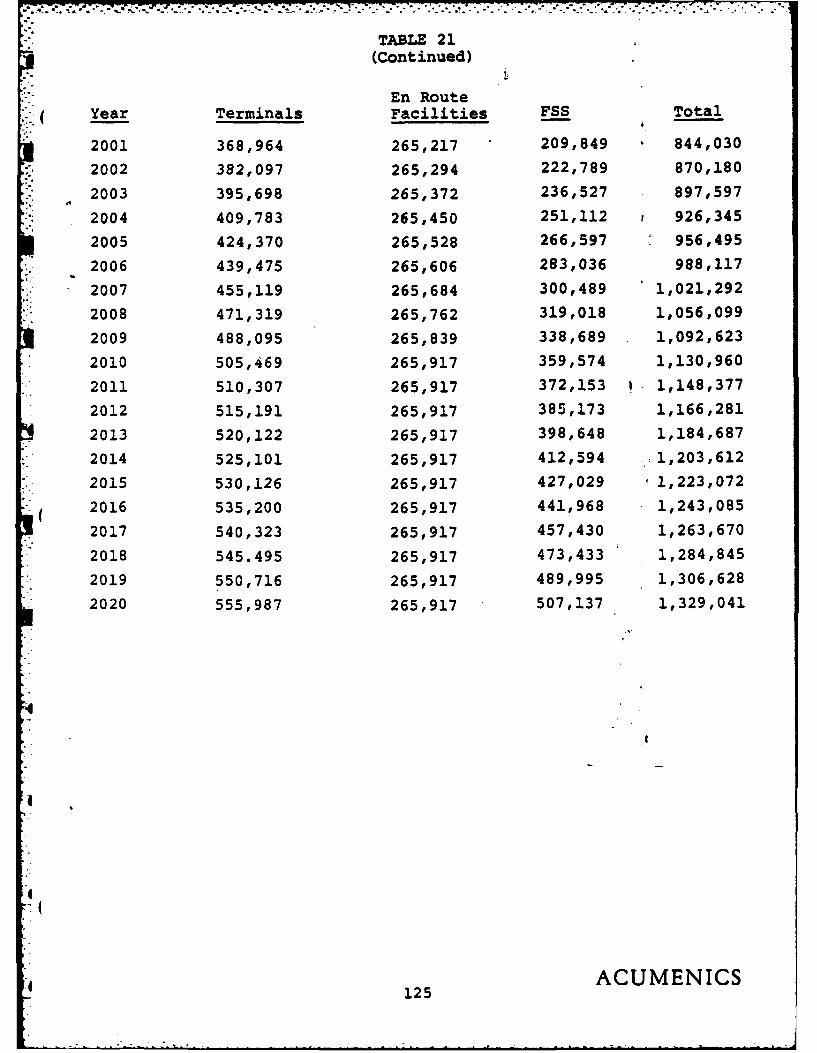
TABLE 21(Continued)
En Route( Year Terminals Facilities FSS Total
2001 368,964 265,217 209,849 844,030
2002 382,097 265,294 222,789 870,180
2003 395,698 265,372 236,527 897,597
2004 409,783 265,450 251,112 926,345
2005 424,370 265,528 266,597 956,495
-. 2006 439,475 265,606 283,036 988,117
* 2007 455,119 265,684 300,489 1,021,292
- 2008 471,319 265,762 319,018 1,056,099
2009 488,095 265,839 338,689 - 1,092,623S 201 505469 2597359,574 1,130,960
2011 510,307 265,917 372,153 1 1,148,377
2012 515,191 265,917 385,173 1,166,281
2013 520,122 265,917 398,648 1,184,687
*2014 525,101 265,917 412,594 -:1,203,612
2015 530,126 265,917 427,029 1,223,072
- 2016 535,200 265,917 441,968 1,243,0852017 540,323 265,917 457,430 1,263,670
2018 545.495 265,917 473,433 1,284,8452019 550,716 265,917 489,995 1,306,628
2020 555,987 265,917 507,137 1,329,041
125 ACUMENICS

assigned to three groups: towered airports ranked among the first
100 in operation, other towered airports, and non-towered airports.
These airports are expected to exceed practical annual capacity
during the decade, to reach saturation or other constraints or to
Sexceed the initial criteria for tower candidacy. Additions to
* terminal facilities and equipment for the purpose of meeting fore-
cast demand have been assumed as shown in Table 22a.
Increases in terminal area facilities will be accompanied by
increases at enroute centers and flight service stations to provide
* for larger volumes of traffic. In the period from 1975 to 1979,
for example, en route center F&E replacement values increased on
( average at 89% of the rate of growth of capital in the terminal
areas (Table 17). Similarly, the growth in Flight Service Station
* F&E replacement costs was 221% of the growth of terminal area
capital investment for the same years. It has been assumed, there-
fore, that each one percent increase in growth of terminal area
capital from 1980 to 1990 will be accompanied by a 0.89 percent
increase in en route center F&E investments and by a 2.2.1 percent
increase in the F&E replacement costs of flight service stations.
These additions are assumed to be in the form of conventional
technology such as is represented in the F&E replacement cost
estimates for 1975 and 1979 in Tables 18 through 20. The additions
* to facilities and equipment at the en route centers and flight
servfce stations that were assumed for the stagflation capital
projects are listed in Tables 22b and 22c.
ACUMENICS126

TABLE 2 2a
STAGFLATION SCENARIOSUMMARY OF IMPROVEMENTS AND ADDITIONSTO TERMINAL FACILITIES AND EQUIPMENT:
(1980 - 1990)(1979 DOLLARS IN THOUSANDS)
A. Additions to Facilities at Airports Total Replacement Value
Exceeding PANCAP Limits by 1990
1. Non-Towered Airports 17,986
2. Towered Airports Not Ranked Amongthe First 100 in Operations 222,945
3. Towered Airports Ranked Among theFirst 100 in Operations (52) 170,820
411,751Total Additions
( B. Improvements to Facilities by 1990
1. Automation at Top-Ranked Airports(152) 212,800
2. Automation at Medium Sized Airports(1.89) 113,400
3. Vortex Advisory Systems 1,292
4. Terminal Information ProcessingSystems 12,344
5. Discrete Address Beacon Systems (90) 198,000
6. Upgraded Airport Surveillance Radars(181) 333,633
*7. Microwave Landing Systems (152)Total 204,925
1,076,394Total Improvements
Source: Figure 1
ACUMENICS

TABLE 22b
STAGFLATION SCENARIOSUMMARY OF IMPROVEM4ENTS AND ADDITIONS TO
EN ROUTE FACILITIES AND EQUIPMENT:1980 -1990
(1979 DOLLARS IN THOUSANDS)
A. Additions Total Replacement Value
1. Increases in Facilities andEquipment Propotional toAdditions to Terminal Areas 524,054
* B. Improvements
*1. Remote Maintenance MonitoringSystems 98,056
2. Upgrading Common Digitizers 10,7543. Direct Access Radar Channel 8,9334. Upgrading Air Route
Surveillance Radars 168,198(5. Discrete Address Beacon Systems 66,000
6. Electronic Tabular DisplaySubsystems 45,310
*7. Additional Data ProcessingCapacity to Meet New Func-tional Requirements 27,600
Total Improvements 448,013
Sources: Figure 2
ACUMENICS128

7-1 % .. . * .. .
TABLE 22c
STAGFLATION SCENARIOSUMMARY OF IMPROVEMENTS AND ADDITIONSTO FLIGHT SERVICE STATION FACILITIES
AND EQUIPMENT1980 - 1990
(1979 DOLLARS IN THOUSANDS)
A. Additions
* Increases in Facilities and EquipmentProportional to Additions in TerminalAreas 232,590
Total Additions 232,590
B. Improvements
1. Replacement of Flight ServiceStations with Automated FlightService Stations 435,240
2. Aviation Weather Processors-
Direct User Access Terminals 787,039
Total Improvements 1,222,279
Source: Figure 3
ACUMENICS129

p Currently the FAA is considering a range of possible improve-
ments to facilities and equipment in the air traffic control system.
It has been assumed that in the stagflation scenario the FAA will
implement the improvements under consideration for the period 1980
to 1990. The MITRE Corporation has recently surveyed and described
the FAA's development plans and this survey24 has been used to
identify the areas in which new technologies will be implemented.
In the terminal areas, improvements have been projected in terms of
the installation of the following systems:
9 Vortex advising systems;
9 Low level wind shear alert systems;
*Terminal information processing systems;
*Wake vortex advisory systems;
* Discrete address beacon systems;
*Microwave landing systems; and
*Upgraded airport surveillance radars.
In addition, a number of processors will be added to the data systems
at the largest terminals to automate certain data analysis and
* communication functions. Seven additional processors are assumed
for each of the major airports in the stagflation scenario, includ-
ing analysis of wind shear and vortex data, aircraft location and
24M. Kay and J. Matney, "Definition, Description and Interfacesof the FAA's Development Programs" a report in three volumesprepared by the MITRE Corporation for the Office of SystemsEngineering M.anagement of the FAA (September, 1978).
ACUMENICS130

conflict data, digitization of radar data, control of data displays
and data entry, and communication of traffic advisories to air-
craft. The facilities and equipment required for these terminal
area improvements are assigned a replacement cost of $1.1 billion
for purposes of the stagflation scenario capital projections, as
* detailed in Table 22a.
* Improvements to facilities and equipment at en route centers
*have been projected in terms of implementation of the following
* systeris:
e Remote maintenance monitoring systems;
* Direct access radar channels;
§ ( * Upgrading air route surveillance radars;
* Upgrading common digitizers;
*Discrete address beacon systems; and
9 Electronic tabular display subsystems.
As in the case of the terminal area projections, processors will
* supplement the data systems of the en route centers to automate
several data analysis and communication functions. Six processors
have been assumed for the projections to 1990, automating the
* detection of minimum safe altitudes, flight path conflicts, and
flight plan conflicts, the metering of traffic, and the formulation
and communication of conflict resolution advisories. The facilities
* and equipment for these improvements have been assigned a replacement
ACUMENICS131

cost of $448.0 million for the purposes of the stagflation capital
projections. The details of the cost projections for en route
center improvements are listed in Table 22b.
Improvements assumied for the flight service stations consisted
* of the installation of sixty automated flight service stations, and
an automated weather information system with direct user access for
* all stations. These improvements total $541.00 million over the
* 1980's, as shown in Table 22c.
Beyond 1990 no comprehensive description of the FAA's capital
* programs has been discovered. Consequently, it is necessary to base
( capital projections on assumptions about the rate of growth of total
capital investment. Total replacement costs for facilities and
* equipment in the FAA's air traffic control system grew more rapidly
during the 1970's than the gross national product.25 However, the
* F&E annual growth rate exhibited a slight declining trend to the
extent any trend can be identified. For purposes of capital projec-
tions annual growth rates in M&E replacement costs from 1970 to 1980
shown in Table 17, have been fitted to a Linear model, using time
as the independent variable. The trend has been extrapolated
through the forecast period (1980-2020). For the decades after
1990 the annual growth rate at the mid-point of each decade was
adopted as representative of the growth in ATC facilities and
25 For example, compare Table 17 of this report with Table 23 ofthe FAA Aviation Forecasts: FY 1980-1981, Office of Aviation Policy(September, 1979).
4 ACUMENICS132

(
equipment investment during that decade. The annual growth rates
in total ATC facilities and equipment are therefore assumed to be:
Stagflation ScenarioTotal F&E Growth Rates
Decade Annual Rate of Increase
1990-2000 1.04932
2000-2010 1.03279
2010-2020 1.01627
The rate for the period 1980-1990 forecast by this method is 1.06585,
which corresponds closely to the increases resulting from aggregation
of the individual improvements and additions actually assumed for the
S( stagflation scenario and shown is Table 22a.
The growth rates beyond 1990 for facilities and equipment in the
terminal areas, the en route centers, and the flight service stations
have been assumed to bear the same relation to each other as they
* did in the period 1975 through 1979. That is, each percentage
increase in terminal area F&E replacement costs has been accompanied
by a 0.89 percent increase in en route center F&E costs, and 2.21
percent increase in flight service station F&E costs.
Finally, the projected F&E values shown in Table 21 represent
the amount of capital consumed annually, assuming an average depre-
ciation period of 14 years for all conventional ATC technologies.
I
ACUMENICS133

Balanced Growth Scenario: Capital Projections
The capital projections for both the balanced growth scenario
and the rapid growth scenario are based upon the assumptions about
conventional technologies adopted in the stagflation scenario. The
projections differ in two principle respects. First, the balanced
growth and rapid growth scenarios assume that a satellite - aided
communication system will replace conventional navigation and commun-
ication technologies. Second, total investments in ATO facilities
* and equipment grows faster in the balanced growth and rapid growth
scenarios than in the stagflation scenario.
For the balanced growth scenario (Table 23) it is assumed that
( conventional technologies are employed to the year 2000. The decade
from 2000 to 2010 will see the gradual replacement of conventional
communication and navigational equipment with a satellite-aided
system. By 2010 the replacement will be complete. The facilities
* and equipment affected by the change can be identified by reference
to Tables 18, 19 and 20 as follows:
o all the navigation aids associated with the terminal areas(Table 18);
o all but five of the air route terminal control centers* and associated equipment (F&E replacement costs under
the heading "centers" in Table 19);
o a proportion of the surveillance facilities and equip-ment associated with the en route centers (18/23, seeTable 19);
o all of the navigation aids associated with the en routecenters (Table 19);
ACUMENICS134

i](* all of the communication facilities and equipment as-
sociated with the flight service stations (Table 20).
" all of the 318 flight service stations themselves, butno other facilities and equipment categories underthe heading "stations" in Table 20.
The projections for capital growth of conventional technology have
been reduced to eliminate the replacement values originally associa-
ted with these F&E categories and the subsequent growth attributable
to them. The reductions can be seen under the headings for terminal
*- areas, en route Facilities and flight service stations from 2000 to
2010 in Table 23. Reductions have been assumed at constant annual
proportional rates.
( In place of conventional communication and navigation facil-
ities, a satellite system will be implemented in the balanced growth
scenario between 2000 and 2010. The system itself will consist of 24
- orbiting satellites which locate aircraft by altitude, latitude,
. longitude and velocity (the GPS system); one communication and data
satellite in geosynchronous orbit (the S/D satellite); and associated
ground stations and data processing facilities. In Phase I form
orbiting satellites will provide limited aircraft positioning infor-
*- mation, using communication and data channels leased from commercial
satellites. In phase II a system of six orbiting GPS satellites will
replace the original four, and an experimental set of geosynchronous
satellites will provide communication and data channels. During the
course of Phase I and Phase II, the largest 100 terminal areas will
receive additional data processing and communication equipment, a
network of calibration stations will be established to maintain
ACUMENICS135

TABLE 23
BALANCED GROWTH SCENARIOANNUAL CAPITAL CONSUMPTION
AIR TRAFFIC CONTROL, SELECTED FACILITIESAND EQUIPMENT1980 - 1990
(2979 DOLLARS IN THOUSANDS)
En Route Satellite
Year Terminals Facilities FSS System Total
1980 97,340 144,936 32,851 -0- 257,127
1981 106,004 152,244 37,200 -0- 106,004
1982 115,438 159,921 42,125 -0- 317,484
1983 125,713 167,985 47,702 -0- 341,400
1984 136,902 176,455 54,017 -0- 367,374
1985 149,087 185,352 61,169 -0- 395,608
1986 162,356 194,698 69,267 -0- 426,321
1987 176,806 204,516 78,437 -0- 459,759
1988 192,543 214,828 88,821 -0- 496,192
• 1989 209,680 225,660 100,580 -0- 535,920
" 1990 228,342 237,039 113,896 -0- 579,277
* 1991 245,235 251,468 127,678 -0- 624,381
1992 263,377 266,775 143,127 -0- 673,279
" 1993 282,862 283,013 160,445 -0- 726,320
1994 303,788 300,241 179,860 -0- 783,889
1995 326,262 318,516 201,623 -0- 846,401
1996 350,399 337,905 226,020 -0- 944,324
* 1997 376,322 358,473 253,368 -0- 988,163
* ACUMENICS136

TABLE 23(Continued)
En Route SatelliteYear Terminals Facilities FSS System Total
1998 404,162 380,294 284,026 -0- 1,068,482
* 1999 434,062 403,442 318,394 -0- 1,155,898
2000 466,174 428,000 356,920 -0- 1,251,094
2001 494,746 451,538 397,892 -0- 1,344,176
2002 525,068 476,370 443,567 -0- 1,445,005
2003 557,250 505,568 494,485 -0- 1,554,303
2004 591,403 530,206 551,248 17,429 1,690,286
2005 627,650 559,364 614,527 25,582 1,827,123
* 2006 666,118 590,126 685,070 37,550 1,978,864
2007 706,945 622,580 763,711 55,115 2,148,351
2008 750,273 656,819 851,379 80,898 2,339,369
2009 796,257 692,940 949,111 118,742 2,557,050
2010 845,059 731,048 1,058,062 117,286 2,808,455
* 2011 872,417 729,154 936,087 217,791 2,755,449
2012 900,660 727,265 828,174 272,155 2,728,254
2013 929,818 725,382 732,701 340,090 2,727,991
* 2014 959,920 723,502 648,234 424,983 2,756,639
2015 990,996 721,628 573,505 531,066 2,817,195
2016 1,023,079 719,759 507,391 663,630 2,913,859
2017 1,056,200 717,895 448,898 829,284 3,052,277
2018 1,090,393 716,035 397,149 .1,036,288 3,239,865
2019 1,125,693 714,180 351,365 1,294,965 3,486,203
2020 1,162,136 712,330 310,859 1,161,211 3,803,536
ACUMENICS137

the accuracy to the position measurements of the GPS satellites,
* and a control center including data processing facilities will be
constructed. It is assumed that the Phase I and II programs will
be implemented between 2000 and 2010 and that the F&E replacement
* values will total $1.2 billion in 1979 dollars. Details are shown
* in Table 23a.
Phase III of the satellite-aided communication and navigation
system will be in place by the year 2010. Phase III is the system
* in its completed form. Additional F&E investments for phase III
* will include the full complement of 24 GPS satellites, a new S/D
satellite, a system of ground stations to allow the satellites
and the aircraft to link with the earth, and an expansion in the
capacity of the control center (see Table 23a for details). It has
* been assumed that the F&zE costs for the three phases are cumulative.
The replacement costs for the facilities and equipment added for
Phase III will be approximately $2.3 billion, bringing the total
to $3.4 billion.
The rate of capital consumption for the satellite based tech-
nologies is more rapid than for conventional technologies. An
* average useful life of seven years has been assumed, which is con-
sistent with the lives estimated for satellite systems currently in
place *26
26See for example "RCA Advances Data for Third Domestic Commun-ications Satellite," New York Times (December 5, 1978), p. D7.
ACUMEN ICS138

:(
TABLE 23a
Capital Cost Assumptions for the SatelliteBased Comunications and Navigation System
A. Additions to Facilities and Equipment in the First Decade
o Phase I - Ground positioning satellite(GPS) system, including four orbitingsatellites, delivery, spares andmonitoring facilities:(l) $355 million
o Phase IT - GPS system, including sixorbiting satellites, delivery,spares and monitoring facilities: 505 million
o Modifications to equipment at 100largest terminal areas 0 $10 million: 100 million
o Development of a 69-transpondersurveillance/data (S/D) satellitefor use in conjunction with the
( GPS system: (2) 100 million
o Network of calibration stations(1000 stations 0 $50,000 (3): 60 million
o National Control Center for S/Dsatellite operations and GPS system: 100 million
- TOTAL $1220 million
B. Additions to Facilities and Equipment in the Second Decade
o Phase III - GPS system, including afull complement of 24 orbitingsatellites, with delivery, spares andmonitoring facilities: $2010 million
o Modification to equipment at 300additional terminal areas, 0 $10million: 300 million
o Delivery of 69-transponder S/Dsatellite in fully operational form,with spare: 100 million
ACUMENICS139

(7
TABLE 23& (Continued)
Capital Cost Assumptions for the Satellite
Based Communications and Navigation System
e Network of ground stations for inter-connection of satellite, ground communi-cations networks (1000 stations$100,000): 100 million
*Additional capacity for the S/S controlcenter: 50 million
TOTAL $2460 million
(1) GPS system costs estimates are based upon a contract be-tween Hughes Communication Services, Inc. and the FCCto build and launch four space satellites for commu-nication purposes. The contract includes maintenance,one spare satellite, and two moveable earth stationsand extends for a term of five years. See New YorkTimes, (December 5, 1979), page D2.
(2) The RCA Corporation's SATCOM 3 communication satellitehas 24 transponders and costs $50 million. To accountfor the increase in the number of transponders, andthe increased complexity of the tasks to be performed,the S/D satellite has been assumed to require $100million for development and design and $100 millionfor final delivery, with one spare. See New YorkTimes (December 11, 1980) page A21.
(3) Currently, small receivers for use with RCA's SATCOMsystem range in price from $10,000 to $40,000 (seeNew York Times (October 28, 1979) at pp. 34-34)Other reported earth station costs range up to$200,000 per unit. (See for example, New York Times(November 23, 1980). The calibration stationsfor the GPS system will perform both transmissionand receiving functions, and will therefore bemore expensive. Likewise the ground stationswill perform a range of functions that will in-crease their costs above the minimum cost forreceivers.
ACUMENICS140

The rate of growth in the system has been assumed, for purposes
of the balanced growth scenario, to be a function of growth in the
Gross National Product. In the period 1970 to 1980 the compound
annual growth for ATC facilities was approximately 104.7%/ of the
* annual growth for GNP.27 The average compound annual rate of
growth in GNP forecast by the FAA for the balanced growth scenario
(i.e. the "baseline" case) is approximately 102.9%/1. The growth in
* ATC facilities and equipment in the balanced growth scenario has
been projected at a rate proportional to the historical relationship
of ATC facilities and equipment replacement costs to GNP. The
* annual rate used or total F&E replacement costs in the balanced
growth scenario is approximately 107.7%.
The growth rates for the terminal areas, en route centers and
flight service stations are assumed to bear the same relationship
to each other as they did in the stagflation scenario. That is, for
each one percent increase in terminal area replacement values, there
will be a 0.89 percent increase in values for en route centers and
a 2.21 increase in values for the flight service stations. The
satellite facilities are assumed to grow at the same rate as the
total of the conventional technologies.
27See Table 23 of the FAA Aviation Forecasts: FY 1980-1981,( Office of Aviation Policy (September, 1979) extrapolated to 2020by Acunenics Research and Technology, Inc. See Scenario Volume.
ACUMENICS141

Rapid Growth Scenario: Capital Projections
Capital cost projections for the rapid growth scenario adapt the
methods employed in the balanced growth scenario with two modifica-
tions. First, it has been assumed that the satellite-based commun-
* ication and navigation system will replace conventional technology
at a very early point in the rapid growth scenario. The satellite
* system is assumed to be fully implemented by the year 2000. Phase
I and Phase II will be implemented between 1980 and 1990, with a
total replacement cost of facilities and equipment in 1990 of
* $1.1 billion. Starting in 1990, conventional navigation and
* communication facilities, identified in the same manner as in the
( balanced growth scenario, will be abandoned. In their place the
* Phase III satellite system will execute ATC navigation and communi-
cation functions. The total replacement value of the Phase III
satellite system is assumed to be $4.9 billion by the year 2000 in
* the rapid growth scenario, increased over the values used in the bal-
* anced growth scenario in order to relate the difference in GNP growth
* for the two sets of projections.
The second modification to the assumptions of the balanced
growth scenario is that the replacement costs of the ATC facilities
and equipment will increase at a compound annual rate of approx-
imately 109.3%. This rate is the product of the average compound
ACUMENICS142

L:(
increase in GNP assumed for the rapid growth scenario 2 8 (i.e.
'"- 104.3%) and the historical relationship of increases in F&E replace-
-- ment costs to increases in GNP between 1972 and 1979 (approximately
104.7%).
Growth in conventional categories of ATC facilities and equip-
ment has been apportioned among the terminal areas, en route centers,
and flight service stations by the same method used in the stagfla-
tion scenario. That is, for each one percent increase in terminal
*area replacement costs, there is an increase of 0.89 percent in en
route center replacement costs, and 2.21 percent for the flight
service stations.
S( Capital consumption has been calculated on the basis of 14
-- years of useful life for conventional technologies, and seven years
*useful life for the satellite systems.
28 See Table 23 of FAA AVIATION FORECASTS: FY 1980-1981 Officeof Aviation Policy (December, 1979) and its extrapolation to 2020.See Scenario Volume.
143 ACUMENICS
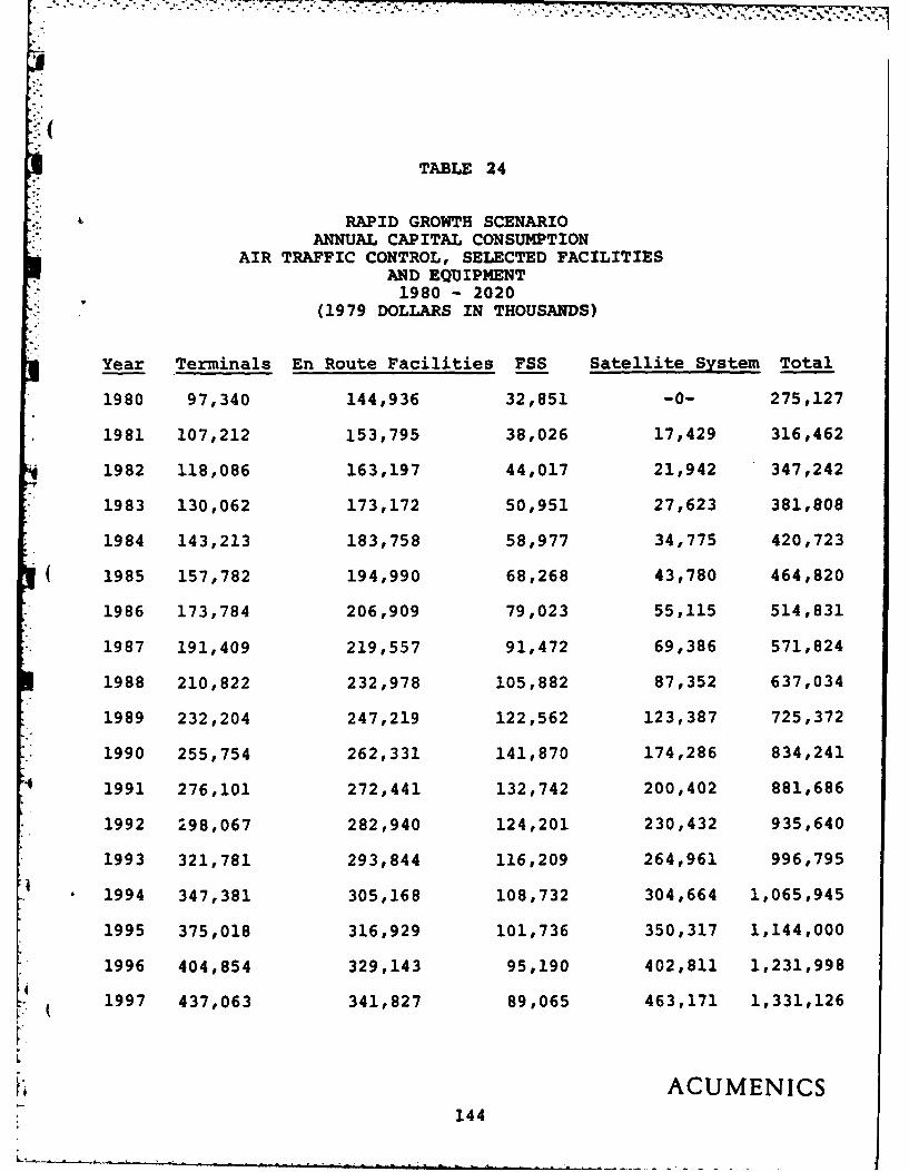
TABLE 24
RAPID GROWTH SCENARIOANNUAL CAPITAL CONSUMPTION
AIR TRAFFIC CONTROL, SELECTED FACILITIESAND EQUIPMENT1980 - 2020
*(1979 DOLLARS IN THOUSANDS)
Year Terminals En Route Facilities FSS Satellite System Total
1980 97,340 144,936 32,851 -0- 275,127
* 1981 107,212 153,795 38,026 17,429 316,462
1982 118,086 163,197 44,017 21,942 347,242
*1983 130,062 173,172 50,951 27,623 381,808
1984 143,213 183,758 58,977 34,775 420,723
( 1985 157,782 194,990 68,268 43,780 464,820
1986 173,784 206,909 79,023 55,115 514,831
1987 191,409 219,557 91,472 69,386 571,824
1988 210,822 232,978 105,882 87,352 637,034
1989 232,204 247,219 122,562 123,387 725,372
*1990 255,754 262,331 141,870 174,286 834,241
4 1991 276,101 272,441 132,742 200,402 881,686
*1992 298,067 282,940 124,201 230,432 935,640
1993 321,781 293,844 116,209 264,961 996,795
1994 347,381 305,168 108,732 304,664 1,065,945
1995 375,018 316,929 101,736 350,317 1,144,000
1996 404,854 329,143 95,190 402,811 1,231,998
1997 437,063 341,827 89,065 463,171 1,331,126
r ACUMENICS144

TABLE 24(Continued)
Year Terminals En Route Facilities FSS Satellite System Total
* 1998 471,835 355,001 83,354 532,576 1,442,746
1999 509,373 368,682 77,972 612,380 1,568,407
2000 549,898 382,890 72,955 704,143 1,709,86
2001 599,206 414,445 83,882 769,325 1,866,858
* 2002 652,934 448,600 96,445 840,541 2,038,520
2003 711,481 485,571 110,890 918,349 2,226,291
2004 775,277 525,588 127,499 1,003,360 2,431,724
*2005 844,794 568,902 146,595 1,096,241 2,656,532
2006 920,544 615,787 168,551 1,197,719 2,902,601
2007 1,003,086 666,536 193,796 1,308,591 3,172,009
2008 1,093,029 721,466 222,822 1,429,727 3,467,044
2009 1,191,038 780,924 256,195 1,562,076 3,790,233
2010 1,297,834 845,282 294,567 1,706,676 4,144,359
2011 1,409,273 911,752 337,504 1,864,662 4,523,191
*2012 1,530,281 983,448 386,700 2,037,273 4,937,702
2013 1,661,679 1,060,783 443,068 2,225,862 5,391,392
2014 1,804,359 1,144,198 507,651 2,431,908 5,888,116
2015 1,959,291 1,234,174 581,648 2,657,028 6,432,141
*2016 2,127,526 1,331,224 666,432 2,902,988 7,028,170
4 2017 2,310,207 1,435,906 763,574 3,171,716 7,681,403
2018 2,508,574 1,548,820 874,876 3,465,319 8,397,589
145 ACUMENICS
145A

7- 17 7-77 -.... . . .7
TABLE 24(Continued)
Year Terminals En Route Facilities FSS Satellite System Total
' 2019 2,723,973 1,670,614 1,002,402 3,786,102 9,183,091
2020 2,957,868 1,801,984 1,148,516 4,136,579 10,044,947
4 ACUMENICS146
( X. AGENCY LABOR IMPACTS
The primary impact of automation on labor is to add or delete
personnel. This section of the report will present estimates of
the agency labor requirem~ents for each scenario, as well as specified
contingencies. These estimates are based on the production functions
developed in Chapter VII.
Estimates of terminal staff (TERM) and center staff (CENT) are
presented for the years 1990 to 2020 for the stagflation, balanced
growth and rapid growth scenarios. The estimates of TERM, as well
as CENT are then compared for all scenarios. In addition, estimates
for the following options have been prepared:
(1) Staff levels under stagflation capital investment with( balanced and rapid growth activity measures;
(2) Staff levels under the balanced growth investment withstagflation and rapid growth aviation activity measures;
(3) Staff levels under the rapid growth investment scenarioand stagflation and balanced growth aviation activities.
* The Scenarios
The official FAA estimates of staff for the period 1970-1990
are shown in Table 25. The historic data 1970-1990 indicates that
the center workforce increased from 10,597 to 10,932 or 3.5%.
The terminal staffing increased from 8,569 to 11,859 or 38.3%
'during the 1970-1979 period. Estimates of staffing from 1980 to
* 1992 incorporate planned technological shifts. From 197') to 1992
the increase in terminal staff is from 8,509 to 16,175 or 88.7%.
The increase for center staff between 1970 and 1992 is 10,597 to
15,121 or 42.6%.
4 ACUMENICS147

. . . .. ... ....... . . .. . ... ........ ....... . . . ....
TABLE 25
CONTROLLER STAFFING
F.Y. TERMINAL CENTERS FSS
1970 8,569 10,597 4,545
1971 9,249 11,328 4,581
1972 9,399 10,772 4,457
1973 9,949 10,682 4,330
1974 10,472 10,764 4,471
1975 10,832 10,813 4,664
* 1976 11,092 11,000 4,892
1977 11,385 10,981 5,054
1978 11,610 10,954 4,966
1979 11,859 10,982 4,9891980 12,653 11,532 5,035
1981 12,653 11,688 5,068
1982 13,363 11,833 5,200
1983 13,695 12,338 5,200
1984 13,983 12,734 5,200
1985 14,307 13,198 5,200
1986 14,597 13,538 5,220
1987 14,867 13,849 5,240
1988 15,000 14,131 5,240
1989 15,396 14,358 5,240
1990 15,659 14,613 5,153
1991 15,916 14,894 4,770
1992 16,175 15,121 4,415
ACUMENICS148

A comparison of center and terminal staff with terminal total
aircraft operations and center IFR aircraft handles for the 1970-
* 1992 period is shown in Table 20. The terminal staff is expected
to increase 88.7% and the operations workload 75.1%. Center staff
is expected to increase 46.6% but workload is estimated to enlarge
by 103.7%. The tentative conclusions drawn from the FAA forecast
and staff level projections is that ceteris paribus the staff magnitude
will increase with more aviation activity. However, technological
change will cause the center staff levels to grow at a slower rate
than terminal staff.
The precceding statement obtains only when new technology is
- ( substituted for extant technology on a continuing basis. If the
extant technology is replaced with the same genre of equipment,
one would expect labor utilization to be less efficient. Inefficient
* labor utilization would result in a staff growth rate proportional
to activity levels.
The stagflation scenario assumes that the agency capital to
2020 is based on extant technology. As such, the level of capital
* may increase, but will not impede an increase in agency staff
proportional to activity levels. The projected agency impact for
d 1990 to 2020 is shown in Table 27. It is anticipated that the number
of terminal personnel will increase from 15,540 to 17,696 or 13.9%.
The size of the center workforce is expected to increase from 14,370
( in 1990 to 21,924 in 2020 or 52.5%.
ACUMENICS149

[.a .'U .* . -
TABLE 26
COMPARISON OF AVIATION ACTIVITY AND STAFF LEVEL INCREASES
TERMINAL CENTER IFRSTAFF AIRCRAFT AIRCRAFT
FY OPERATIONS HANDLES____TERM CENT (MILLIONS) (MILLIONS)
1970 8,589 10,597 56.2 21.6
1992 16,175 15,121 98.4 44.0
n -0
CHAGE 88. 4.6 75.1 103.7
I 1 4
-4
ACUMENICS150

TABLE 27
AGENCY STAFF 1980-2000: STAGFLATION SCENARIO
OBS YEAR STERM SCENT-
21 1990 15539.4 14369.722 1991 15801.5 14768.323_ ".. 1992-- -I-6-77.. 1512 .24 1993 16217.2 15433.125 1994 16371.0 15698.027 - 1995 T184 117.927 1996 16573.2 16093.728 1997 16623.4 16226.3-29 i99----6641.5 T1 -7.5-30 1999 16628.8 16368.931 2000 16586.8 16382.732 200i 16708.7 1684i.033 2002 16804.8 17277.3
( 34 2003 168760 17691:2-5 200 o4 16923 .-4 18083.0 *36 2005 16948.1 18453.037 2006 16951.2 18801.638 2007 '16933.8 91i29.339 2008 16897.3 19436.840 2009 16842.9 19725.041 2010 i677.6- 19994.242 2011 16919.9 20253.7
151 ACUMENICS

It is expected that terminal staff will increase with activity
and center staff will decline under the balanced growth scenario.
That is, centers will be more automated than terminals. The expected
* staffing levels for centers and terminals under the balanced growth
scenario is shown in Table 28. The terminal staff is expected to
* increase from 17,062 in 1990 to 25,131 in 2020 or 47.50/. Owing to
automation, the center staff is expected to decrease from 13,434 in
1990 to 4071 in 2020 or -69.7%.
The rapid growth scenario is expected to result in increased
terminal staff to accomodate growth. Increased automation will
* result in decreased center staff. The estimated staff levels under
the rapid growth scenario are shown in Table 29. Under rapid growth,
terminal staff is expected to increase from 21,636 in 1990 to 31,147
or 43.9%. Center staff is expected to decrease from 10,983 in 1990
* to 2,172 in 2020 or-79.4%a.
A comparison of terminal and center staff levels across scenarios
is shown in Tables 30 and 31. The continued discussion of the staff
levels in the context of aviation activity is in a succeeding section.
The Stagflation Option
The following section includes the staff estimates for the
following conditions:
(a) The agency capital investment is for extant technologyi.e., the capital investment under Stagflation.
- ((b) Aviation activity levels during the forecast periodreflect rapid or balanced growth levels.
ACUMENICS152

7 7 7
TABLE 28
AGENCY STAFF-BALANCED GROWTH
OBS YEAR BTERM BCENT
.-1 1990------17062.1- 13434.32 1991 17687.9 13477.43 1992 18307.0 13478.4
-4-- 1 . . S.. . 8 -7, -- - -343-7-9-
5 1994 19515.6 13356.56 1995 20100.3 13235.67" "1996- -- 206687 1 076.-
8 1997 21218.6 12882.09 1998 21747.6 12653.6
-10- ... -- 9- -2 2 3 5 12394.1
11 2000 22734.3 12106*012 2001 23352.2 11894.8
( .- 1-3 2002-- 23948.544 6,6w3-14 2003 24520.8 11392.715 2004 24850.3 10828.8
--..16- .....2005- -- 2 5280,7- 0429.217 2006 25647.0 9980.918 2007 25935.1 9481.8
_ ~~~--i9, -2008----62 . 9 = - -
20 2009 26201.2 8304.921 2010 2.6130.6 7616.4
' ~~~~~~~----2 ----. 2011---- 6 5 ,- - - T-L- -
23 2012 26897,0 7604.324 2013 27134.3 7463.5
-- 25---- 204-4---27258-.4- 7223.1-26 2015 27258.0 6882.427 2016 27123.1 6445.4
---28 2017------26845.-9---9-24--4--29 2018 26421.5 5338.230 2019 25848.8 4711.4
-- 31- 2020---254-31.4--40.71,232 2021
153 ACUMENICS

(
TABLE 29
AGENCY STAFF-RAPID GROWTH
OBS YEAF RTERM RCENT
---.. -- .1990- 21636.-4 40982,-S-2 1991 22467.4 11118.13 1992 23250.4 11168.1
-- 4-- .--1993----23982. ---. 11132975 1994 24659.5 11013.86 1995 25280.1 10815.2- -7-- .. .. 199-6---258417 1054I.I
8 1997 26342.7 10199.09 1998 26781.8 9796.5
----- ~ -1999 271583- 9342,511 2000 27471.5 8846.512 2001 27984.3 8380.1
.--1t- 2002 -- 28457 , 6 ------ 79-9- -9-14 2003 28891.5 7467.5
15 2004 29286.0 7026.2
-- 6---- 2005----29641.3-- -&59-7-r4-17 2006 29957.9 6182.718 2007 30236.2 5783.119 2008 30476.8 5399.820 2009 30680.3 5033.2
-24--- 2010----30847. - 46@3o722 2011 31021,1 -4364.923 .2012 31160.3 4061.524 2013 31265.9 3773.5
-25--- 2014-------31339 ----- 3500.926 2015 31380.3 3243.427 2016 31391.0 3000.92 .- 20-17---31371.9 . -7-2-,-9-29 2018 31324.2 2559.030 2019 31246.8 2358.2
-31- 2020 --- 31-147.3-----1--4732 2021 .
154 ACUMENICS

TABLE 30
TERMINAL STAFF-ALL SCENARIOS
OBS YEAR STERM BTERM RTERM
---1 - 1990 -15541,4 --7-062-------21636.4
2 1991 15803.5 17687.9 22467.43 1992 16029.5 18307.0 23250.4
---.4 -- 1993 6--121-9,3 ..... - 9!710 23-9820-1-5 1994 16373.0 19515.6 24659.56 1995 16491.4 20100,3 25280.17-- 1996 --.16575.2--8 1997 16625.5 21218.6 26342.79 1998 16643.6 21747.6 26781.8-4 0 . .. .9 9 ..... I" 3 0 #8 - 22253- !581 3-
11 2000 16588.9 22734.3 27471.512 2001 16710.8 23352.2 27984.313- ----.2002 ... - L, .-. . .!9 5 2 4 -
14 2003 16878.2 24520.8 28891.515 2004 16925.6 24850.3 29286.0
-16-----2005 --169-50-, 2 - ---259. 2964-o-3---17 2006 16953.3 25647.0 29957..918 2007 16936.0 25935.1 30236.2
--19......2008 --- 1-4899.4 - 2127 2 30476-.-8--20 2009 16845.0 26201.2 30680.3
21 2010 16773.7 26130.6 30847.52--2 * 2011 -16922.-O -0- -- 26Z8- 5,- 21---23 2012 17056.4 26897.0 31160.324 2013 17177.4 27134.3 31265.9
-25-- -.. 2014 --47285,6 -----24§&,-4 -4 31_9--0-26 2015 17381.6 27258.0 31380.327 2016 17465.9 27123.1 31391.0
-28- -- 2017 - 1-7Z5391 4 -6894 5-v, -- 47429 2018 17601.9 26421.5 31324.230 2019 17654.7 25848.8 31246.8
-31 2020 -1-7698.2 --- 254r1- -1 3 147.4-32 2021
5 ACUMENICS~155

TABLE 31
CENTER STAFF-ALL SCENARIOS
OBS YEAR SCENT BCENT RCENT
1 1-.19-9.0-----436 -7 3434 -3 .. -
2 1991 14768.3 13477.4 11118.13 1992 15123.0 13478.4 11168.14-. ----- 143, -1---434 ,- . 1-132 25 1994 15698.0 13356.5 11013.86 1995 15917.9 13235.6 10815.27-.....1-996---6093,7 --130-76-.8 .- 1-4544.4-8 1997 16226.3 12882.0 10199.09 1998 16317.5 12653.6 9796.5
--- 0 -----4-1-9-9----44368 9---- 1394- 93-42.511 2000 16382.7 12106*0 8846.5
( 12 2001 16841*0 11894. 8380.113 2002 17277.3 11656.3 7919.614 2003 17691.2 11392.7 7467*5
-15-20-4 1 _.- .8 7026.216 2005 18453.0 10428.2 6597.417 2006 18801.6 9980.9 6182.718 2007 19129.3 9481.8 5783.119--- 2008--19436#-8 -.... 8925-2 -....599--8--20 2009 19725.0 8304.9 5033.221 2010 19994.2 7616.4 4683.72 -.. t--'-20 025 -3-7 4... A-5 T----23 2012 20496.3 7604.3 4061.524 2013 20722.6 7463.5 3773.525 -- 20-4- -20933,7 -...9723-r4 --- 350-#9---26 2015 21130.2 6882.4 3243.427 2016 21313.2 6445.4 3000.928 - 20i7---21-483.-3 .29 2018 21641.3 5338.2 2559.030 2019 21787.9 4711.4 2358.231 2020-----21923.8 4071.2 -2.1-7 1w7--32 2021 .
156 ACUMENICS

In essence, this section considers the impacts if the agency invests
technology on the stagflation level and balanced or rapid growth
aviation activity occurs.
Estimates of terminal staff requirements are shown in Table 32.
* If stagflation investment occurs with stagflation growth the terminal
staff will increase from 15,541 in 1990 to 17,698 in 2020 or 13.8%.
- If stagflation investment occurs with balanced growth activity the
terminal staff will increase from 10,512 in 1990 to 56,812 in 2020
or 191.2%. In similar, if the stagflation investment occurs with
rapid growth activity the terminal staff will increase from 33,522
* in 1990 to 138,112 in 2020 or 312%.
( Estimates of center staff requirements are shown in Table 33.
If the stagflation capital investment occurs with stagflation
aviation activity levels, the number of center staff will increase
from 14,370 in 1990 to 21,924 in 2020 or 52.6%. If the stagflation
capital investment is coupled with balanced growth activity measures
then the center staff will increase from 18,812 in 1990 to 67,936
* in 42020 or 261.1%. In similar, if stagflation capital is used in
* conjunction with rapid growth activity the number of center staff
* would increase from 34,737 in 1990 to 245,218 in 2020 or 605.9%.
ACUMENICS157

I
TABLE 32
TERMINAL STAFF-ACTIVITY ALL SCENARIOS-STAGFLATION CAPITAL
oBS YEAR STERM STERMB STERMR
_.1 1990 15541.4 19511.7 335222 1991 15803.5 20419,5 356333 1992 16029.5 21335.9 377724 1993 16219.3 22258,4 399365 i904 16373.1 23183.9 421206 1995 16491.5 24109.7 443207 1996 16575.3 25032.7 465328 i997 16625.6 25949.7 48753-"9 1998 16643.6 26857.8 50980
10 1999 16630.9 27753.6 5320711 2000 16588.9 28634.2 5543312 2001 16710.8 29838.2 58322
( 13 2002- 16807.0 31044:4 6126314 -2003 16878-2 32249*3 -64251-
15 2004 16925.6 33449.3 6728616 2005 16950.3 34641.1 70364I7 ... 2006 -6953.3 35821.2 7348318 2007 16936.0 36986.0 7664119 2008 16899.5 38132,4 7983520 2009 i6845.0 39256.9 83062-21 2010 16773.8 40356.4 8632022 2011 16922.1 42011.6 9087023 2012 1f7656.5 43673.7 9555724 2013 17177.5 45339.1 10038425 2014 17285.6 47004.5 10534926 2015 17381.6 48666.6 11045527 2016 17465.9 50321,9 11570228 2017 17539.2 51967.2 12109129 2018 17602.0 53599.3 12662130 2019 17654.8 55215.3 132295
2020 17698.2 56812.2 138112AC2ME021
4158 ACUMENICS

TABLE 33
CENTER STAFF-ACTIVITY ALL SCENARIOS-STAGFLATION CAPITAL
CBS YEAR SCENT SCENTB SCENTR
1 1990 14369.7 18811.5 34737
2 1991 14768.3 1995097 375793 1992 15123.0 21116.4 40507
4 1993 15433.1 .22276.0 43517
5 1994 15698.0 23432.5 466036 1995 15917.9 24579.8 49761
7 1996 16093.7 25711.9 529848 i997 i62-26.3 26822.6 562689 1998 16317.5 27906.4 59607
10 1999 16368.9 28957.3 62996
11 2000 16382*7 29970,1 6643012 2001 16841.0 31847.4 7195413 2002 17277.3 33758.5 77782
14 2003 -17691.2 35697.5 8392115 2004 18083.0 37658.6 90380
16 2005 18453.0 39636.0 97167
17 2006 18801.6 41623.8 10429218 2007 19129.3 43616.0 111763
19 2008 19436.8 45607.1 11958720 2009 19725.0 47591.6 12777521 2010 19994.2 49563.7 13633422' 2011 20253.7 51539.5 14533123 2012 20496.3' 53494.9" 15472424 2013 20722.6 55425.1 16452125 2014 20933.7 532. 174733.5 2142r-, 57326*4 143
26 2015 21130.2 59194.6 18536827 2016 21313.2 61026.7 196436
28 2017 21483.3 62819,4 20794529 2018 21641.3 64570,1 21990530 2019 21787.9 66276.4 232325
31 2020 21923.8 67936,3 24521432 2021 . o
159 ACUMENICS

The Balanced Growth Option
This section considers the agency impacts if the balanced
growth scenario capital is in place and rapid growth or stagflation
aviation activity prevail. Estimates of terminal staff for the
above contingency are included in Table 34. If stagflation
activity levels occur then the number of terminal staff (BTERUS)
* will decrease from 13,503 in 1990 to 7,575 in 2020, a change of
43.8%. If the rapid growth scenario activity levels prevail, then
the number of terminal staff (BTERMR) will increase from 29,765 in
* 1990 to 62,647 in 2020, an increase of 110%.
The estimates for center staff are included in Table 35. If
.( stagflation activity levels prevail the number of center staff
(BCENTS) will decrease from 10,059 in 1990 to 1,200 in 2020, a
change of 87.9%. If rapid growth activity occurs, then the center
staff (BCENTR) will decline from 25,981 in 1990 to 16,161 in 2020,
a change of 37.7%.
The Rapid Growth Impacts
This section presents the agency impacts if the rapid growth
scenario technology is adopted and activity levels are at the
balanced growth or stagflation scenario levels. Estimates of
terminal staff requirements are presented in Table 36. The number
of term staff (RTERMS) for stagflation activity levels will decrease
from 9,592 in 1990 to 3,541 in 2020, a change of 63.1%. If balanced
growth activity levels prevail, the terminal staff level (RTERMB)
ACUMENICS160
a -' i " % m .wfi ft ' . 'i - _ ' . . .

TABLE 34
TERMINAL STAFF BALANCED GROWTH CAPITAL-RAPID AND STAGFLATION ACTIVITY
01S YF-4 JTERMl ITME' ITMPP1 19.96 13583,.1 17962, 29765 .9
2 .1.M 1359.66 17687.9 3155.'I3 1,9 0443.2 t830 ,0 3-297.74 19 3. 3661.? 18917.0 P96.55 1.9 !3647.6 19515.6 36058.76 I.s 31922 29186.3 3 97 19%.' 13527.2 20668.7 34.99.58 1"? !3424.4 21218.6 40581.69 199.8 13295.8 21747.6 42934.31. 19M, 13143.4 2 23.5 43453.611 29M 129 69.2 22734.3 44841.212 2101 112865.8 23352.2 46517.?
( 3 29W 12742.4 23W.5 4817f.414 2M 126M.6 2452..8 4984. 715 ?904 1233A.? 04856.3 5m98.816 290 1222.7 2.20.7 523M.117 2011 11894.2 25647.9 53691.618 268? 11616.4 ES5935 .1 54866.919 Me0 11315.7 26127.2 a 545835.629 2W.89 18'977.2 26201.2 5662M.121 2918 10594.7 'f6130.6 57986.322 2811 160426.2 26558.5 58711.723 2912 18229.0 26897.1 68167.324 2913 1082.1 27134.3 61442.625 2014 9744.6 27258.4 62562.726 2915 9456.1 27258.6 63315.?27 29t6 .136.6 27123.1 63847.7
28 2017 8786.7 26845.9 64068.5-9 2918 8407.9 26421.5 63952.6
CopY available to DTIC d ;cPermit fully legible reproducticn
161 ACUMENICS

--- -. , - - . ---, . -* -.- -. ,- . . ,-. • -.. -" - . - . " ,. "
TABLE 35
CENTER STAFF BALANCED GROWTH CAPITAL-RAPID AND STAGFLATION ACTIVITY
03S YER. KUM CTIr
1 1998 18859.4 13434.3 25%1.22 1 9 751.9 134774 2659H.33 1992 9417.1 13472.4 27133,94 1993 9866.2 13437.9 2M86.5 1,4 8686.1 13356.5 27951.36 1995 049.9 13235.6 2 ~~c7 1,., 798i5.e 13876.8 28429.88 19 798.1 2882.8 2858.29 19M 7118.. 1265.6 2851.610 199, 6.2 12.34.1 2861.311 29M 6328. 12186.8 28462.412 298! 6688.8 1189.8 247.3
( 13 282 56762 11656.3 2859.914 2863 5368. 11392.7 29534.915 U4 4924.7 1882. 238. 316 2905 4587.6 18428.2 27328.617 286 t258.6 998. 9 26768. -918 208? 3912.2 941.8 2665.519 2898 3579.8 8925.2 25135.428 28W9 3224.6 8384.9 23989. 82! 2810 2872.6 7616.4 22581.822 2811 286.2 7652.1 2329%723 2012 2713.7 7684.3 23794.424 2613 2594.32 74623 24013. 925 2814 2448.9 7223.4 23912.226 2815 2276.2 6882.4 23454.127 2816 2882.2 6445.4 2262.723 27 1871.2 5924.4 2142..429 2818 1658.9 5338.2 19987.938 2819 1426.31 471f.S ""2 4
Copy avoilable to DTIC does not
petmit fully legile epoduc
162 ACUMENICS

_--..- ;-: - 4 . - -- 1-... 777.- -. 7,7 777- - -7 - 7N
:?(TABLE 36
TERMINAL STAFF RAPID GROWTH CAPITAL-BALANCE AND STAGFLATION ACTIVITY
f. lS YEAF RT!WS PTU! RTEP.
I 19 5 9i.32 12201.8 216,6.'2 !991 '3343.03 2464. 1 22497.43 1992 Mi8.i# 12",T1.4 2M15.4
4 IM9 9241.88 12919.9 2.3982.5 1.94 9872.98 1219.4 2465.5
1995 0880.41 13273.! 2!29. 17 1,9.. 9667.97 134e. 9 25,41.78 199? 2437.61 13515.7 26?42. 79 1992 e191.76 13592.6 267LP.8
18 1?9 7932.6 1'639, E 271!8.31 . 7663.24 13254,9 27471.51 2 2881 7455.21 13768.9 ZM~4.3
(13 28N2 7040.62 13868.9 2B'57.614 2883 7.21. ~ 3915 2884 6797.S2 1397. 6 92, 6.816 2M0 W572.31 1402. 7 2%64!.317 2N6 E.145.7 1 '4.. 2997.918 2A97 6119.2 ]3P85,.4 322.219 2 8 5893.5Z 13943.8 38476.8. 2P99 5669.88 143888.9 1268t. 321 2918 .448. " 1379..1 30847.522 leall 5239.1 137!1.7 31P2!.!23 291k 5830.8Se 136f6. 6 [email protected] 201A 4827.? !3482.7 'I.925 2814 462..29 1338.r.7 3'239 .:'6 2915 4433.8 31et.6 313'8.3?7 2816 4244. l 1396. 5 3'39!.
'29 2817 4968.20 296. !:3.1 929 ,E1 8 . 1881,7 21. 3114.2
163 ACUMENICS

will decrease from 12,203 in 1990 to 12,166 in 2020, a small
*- change of 0.3%.
Center staff requirements are shown in Table 37. If stag-
flation activity occurs then center staff (RCENTS) levels will
decrease from 3,945 in 1990 to 132 in 2020, a change of 96.6%.
*The center staff level (RCENTB) for balanced growth activity levels
will decline from 5,392 in 1990 to 490 in 2020, a change of 90.9%.
,, Flight Services Station Personnel
The impact of technology on flight service station staff is
- shown in Table 38. The staff level estimates are for congruent
activity and capital. If the existing technology is continued inuse under the stagflation scenario, the flight service personnel
*7 (SFSS) will increase from 4,714 in 1992 to 22,698 in 2020; a net
increase of 382 percent. If the agency went in balanced growth
technology, the number of flight service staff (BFSS) will decrease
*" from 4,191 in 1992 to less than 100 in 2020. If rapid growth
activity occurs in conjunction with the use of rapid growth tech-
nology, the workforce (RFSS) is expected to increase from 1,690
in 1992 to 3,800 in 1992, then decrease to 109 by 2020.
Two non-congruent condition sets of staff estimates are shown
in Tables 39 and 40. The data in Table 39 contrasts the following
conditions: balanced growth activity with balanced growth tech-
nology (BFSS), and stagflation activity with balanced growth tech-
nology (BFSSS). As noted above, for the balanced growth, congruent
164 ACUMENICS

Z- 7 77 77 7 77. 77
1
condition staff is expected to diminish from 4,191 in 1992 to
less
than 100 in 2020.
I balanced growth technology is used with stagflation
activitY, the FSS will be fully automated by 2003.
If rapid growth technology is fully employed with either
balanced growth (RFSSB) or st&gfl
atiO n activity (RFSSS), their
col e ul automated by 1092.
1• flight service stations could be fully
,.-
ACUMENICS165

TABLE 37
CENTER STAFF RAPID GROWTH CAPITAL-BALANCE AND STAGFLATION ACTIVITY
1.19 YERF PCENTS RET CVPM
2 1991 3762.7S 5336.68 I18. 13 IM9 35161.34 245. 57 1.16E.1I4 19. 3^044.6t 5119.6? 111?2.75 199N ?JVU.5 49cae.9 19186 99 l 2682.27 4772.13 1801.2
p"45.91 4556.46 18541.12448.46 431 12199.9
9 193e 2!79.49 4861.98 974,.5!B 1999 1956.64 3792.21 9:342.5
M 2)8 !7A3.8 3512.82 P846.512 2P1 1,94.66 3255.55 ME I! 3 2.42 '382.7 e887. 43 ~ 114 2M3 12-27.8? Mi7. 4 747.5
E5M84 886.6 2544, 1 MERE.216 3885 268.44 2"1. '5 65,7,:7 HK8 847.23 "i8 25 61ET. 71I 288N 746,27 191i.43 5.119 289 656.22 16. 94 5399.928 2?H9 576,19 16H.62 983?.221 E916 585.2 1481 A,
22 2811 49.2 611.23 mA??.23 M92 ^89.F3 !!St.'s W 15.4 2113 Z41.12 e, 711 525 2014 9 i 9699 3 .26 2811 26.2 6.3 30j?.!427 60W6 2. 7.23 228 20117 Q99.2 69.6 277t 0
W9 It1 d 17. 61.E W, 9.29 219 151.4C 58. 49 2 E. 2
r- b- 2; 13J.'34 S8.6 P.
166 ACUMENICS
------------------------------

TABLE 38
FSS PERSONNEL ALL SCENARIOS
3 YEAR SF35 1Fss EFSS
K 1992 4714.5 4199.72 1689.732 1993 474.44 3523.-48 2386.523 1994 4705.9 2907.48 3045.194 1995 4602.9 2391.13 3549.685 1996 4442.9 1878.79 3866.466 1197 4234.6 1473.66 3771.957 1998 3965.7 1138.22 3497.858 1999 3708.4 866.30 3053.279 200 3411.3 649.42 2325.66
16 20!1 3673.4 303.36 2328.5811 2002 3914.3 304.72 2479.68012 203 4129.3 296.43 2303.7413 2 04 4314.0 168.76 2248.2914 2665 4465.6 115.19 2681.9915 206 4579.9 75.96 1894.2216 2287 4657.0 48.10 1694.2417 2:8 4695.7 29.32 1496.5618 2069 4696.5 16.52 1290.64o19 21 4660.3 12.92 1160.34
26 2:11 5629.6 24.72 927.9321 2612 8738.3 99.42 771.4322 2613 8036.7 119.35 632.4823 2614 9502.3 192.73 511.52Z4 2015 11159.8 245.82 48.4425 2616 13621.4 245.34 321.9926 2017 15097.9 192.29 236.5427 2618 17398.2 126.42 192.6228 2619 19930.2 61.85 146.6829 2626 22698.4 26.87 1e9.8w -
36 2021
I
167 ACUMENICS

TABLE 39
% BALANCED GROWTH CAPITAL-BALANCED GROWTH AND STAGFLATION
obs YEAR BFSS BFSS
1 1992 4190.72 351.1322 1993 123.48 270.2243 1994 2907.48 204.9454 1995 2391.13 153.5125 1996 1878.79 113.1466 1997 1473.66 82.4567 1998 1138.22 59.3578 1999 866.30 42.2309 2000 649.42 29.675
10 2001 503.36 21.61611 202 384.72 15.56412 2003 290.43 11.09513 2004 168.76 6.10114 2005 115.19 3.94915 2006 75.96 2.47416 2007 48.10 1.49117 2008 29.02 0.85818 2009 16.52 0.46619 2010 12.92 0.34920 2011 24.72 4.63921 2012 59.62 1.48022 2013 119.35 2.4623 2014 192.73 4.42024 2015 245.12 5.42925 2016 245.30 5.22326 2017 192.29 3.95227 2018 120.42 2.39228 2019 61.45 1.18529 2020 26.87 0.50030 2021
I
168 ACUMENJCS

TABLE 40
RAPID GROWTH CAPITAL-OTHER SCENARIO ACTIVITY
OBS YEAR RFSS RFSS3 RFS58
1 1992 1689.73 6.177478 2.115432 1993 2386.52 0.187452 2.441043 1994 3048.19 0.181836 2.376304 1995 3549.68 0.163128 2.50498
5 1996 3800.46 0.136331 2.260836 1997 3771.95 0.106913 1.908297 1998 3497.88 0.079229 1.517318 1999 3053.27 0.055850 1.144209 2000 2525.66 0.037675 0.82343
10 2001 2528.58 0.031040 0.7218911. 2002 2479.S0 0.025264 0.6236612 2003 2383.74 0.020319 0.5312013 2004 2248.29 0.016154 0.4462514 2005 2081.99 0.012697 0.3699015 2006 1894.22 0.009870 0.3026416 2007 1694.24 0.0075;9 0.2444817 2008 1490.58 0.005774 0.1950718 2009 1290.64 0.004347 0.1537719 2010 1100.36 0.003239 0.1197820 2011 927.93 0.002399 0.0926121 2012 771.43 0.001760 0.0708122 2013 632.48 0.001279 0.0535623 2014 511.62 0.000921 0.0400924 2015 408.44 0.000657 0.0296925 2016 321.90 0.000464 0.0217726 2017 250.54 0.000325 0.0158027 2018 192.62 0.000226 0.0113528 2019 146.08 0.000155 0.0080629 2020 109.85 0.000106 0.0056930 2021
1
169 ACUMENICS

XI. MEASUREMENT OF PRODUCTIVITY
The basic measure of technology and labor productivity is
- the system product divided by the labor necessary to provide the
product. As noted previously, system product is a function of the
factors of production (i.e., labor (L) and capital (C), or
Q = f (C,L). The formulation employed in estimating system product
is Q = A& L8 . Thus, the ratio of product to labor provides and
indicates the average product as well as the general efficiency of
*the technology.
The system components, product and labor are:
System
Component Product Labor
terminals operations (TOPS) terminal staff (TERM)
centers aircraft handled center staff (CENT)(AIRHAND)
FSS contacts (CONT) flight service staff (FSS)
The average product for each component is then:
System Average
Component Product
terminals TOPS/TERM
centers AIRHAND/CENT
FSS CONT/FSS
Both the numerator and denominator of the average product for each
system component has been estimated. rhe numerators are the forecast
estimates provided in the scenario section. The denominator pro-
jections have been developed using the production function construct.
ACUMENICS170

(
The average product measure (APM) indicates staff productivity
since it indicates the level of product produced by each staff
member. The APM also indicates the relative impact of technology
since the average reports the productivity of staff for a given
technological construct. Thus, the APM indicates for the same
time period, whether more or less product is produced under a
given technological regime. Thus, if the APM for a given time is
the same across scenarios, the technology allows one to accommodate
growth, but offers no unit labor savings. However, if the APM is
greater under balanced growth then compared stagflation the tech-
, ~nology is labor saving. An example of non-labor saving and labor
saving APM's are shown in Table 41. The non-labor saving condition
occurs when stagflation APM = balanced growth APM = rapid growth
APM. The labor saving effect of technology is shown in Row B where
stagflation APM balanced growth APM rapid growth AM. Under the
Row A conditions, the relative effects of balanced and rapid growth
technology compared to stagflation technology is 1.00 or
Balanced growth APM = 6000 = 1.0Stagflation APM 6000
Rapid growth APM = 6000 = 1.0Stagflation APM 6000
4 The relative efficiency of technology for balanced and rapid
growth under row B conditions are:
Balanced growth APM = 8000 = 1.33Stagflation APM 8000
Rapid growth APM = 12,000 = 2.0Stagflation API 6,000
ACUMENICS171

TABLE 41
TOPS/ TERM
SCENARIO
Stagflation Balanced Growth Rapid Growth
(S) (BG) (RG)
A 6000 6000 6000
B 6000 8000 12,000
ACUMENICS172

The above indicates that for the given scenario activity levels
• :the staff can produce 1.33 operations under balanced growth for
each 1.00 generation for stagflation.
Comparative APM estimates are provided for two generic sets
of conditions. A set of estimates is provided where the scenario
activity and capital estimates are congruent. For example, stag-
flation activity and capital were used to estimate staff. The
second set of estimates are noncongruent. The estimates examined
the impact of using one scenario activity level with another
*scenario's capital. For example, estimating staff using stagflation
activity and balanced growth capital, the second set of estimates
provides impact measures for a non-optimal allocation of resources.
As such, the second set of estimates provides a basis of comparing
- the efficiency of different scenario technology using a constant
activity basis. Thus, the congruent and noncongruent conditions
allow the calculation of a series of if - then estimates. The fol-
lowing provides a summary of the if - then relations.
Congruent
If S capital and S activity then S workforceIf BG capital and BG activity then B workforceIf RG capital and RG activity then R workforce
Noncongruent
If S capital and BG activity then S workforce B
If S capital and RG activity then S worKforce R
ACUMENICS173

-. ... . .. . . . . . . . . ..-- ' - -' '-. - - - .'.. . . . . . . " " . . . . . ." "
Ii
If RG capital and BG activity then B workforce R
*If RG capital and B activity then B workforce R
If RG capital and S activity then R workforce S-If RG capital and BG activity then R workforce B
when workforce equals TERM, CENT, FSS as appropriate
A
!i
ACUMENICS174

(
The following table provides a summary of the different conditions
* embodied in congruent and noncongruent estimates.
Congruent
Scenario Stagflation Balanced Growth Rapid Growth(S) (BG) (RG)
Conditions
Activity S BG RG
Capital S BG RG
Noncongruen t
Scenario Stagflation Balanced Growth Rapid Growth(S) (BG) (RG)
Conditions
Activity BG RG S RG S BG
Capital S S BG BG RG RG
(
ACUMENICS175

7.7767;
XII. THE IMPACTS IN CONTEXT
The previous sections have presented the impacts of tech-
nological change in terms of agency workforce level. This section
will view those staff estimates in the context of scenario vari-
* ables for discrete years. The years of interest are 2000, 2010, and
2020.
Summary statistics for the stagflation, balanced growth, and
*rapid growth scenarios are presented in Tables 42, 43, and 44. The
statistics in the summaries include: total operations, local opera-
* tions, itinerant operations, aircraft handled, IFR departures, overs,
total general aviation (GA) aircraft, single engine GA aircraft,
multiple engine GA aircraft, total air carrier, total pilots, private
pilots, transport pilots, student pilots, terminal staff, center
staff, GNP, DPI and employment. In addition to the descriptive
* estimates, several descriptive statistics are also provided, including
* messages/operation, messages/aircraft handled, total operations
/aircraft, total operations/terminal staff, total aircraft handled/
* center staff, total operations/total pilots.
* Stagflation Scenario
* The stagflation scenario (Table 42) is a slow growth environ-
ment with the agency capital investment based on extant technology.
* Under the stagflation scenario total annual operations will be 09.9,
I 107, and 111 million in 2000, 2010, and 2020 respectively. The
total aircraft handled will average from 44.4 million in 2000 to
* ACUMENICS176

TABLE 42
S( Stagflation Scenario
TIME/VARIABLE 2000 2010 2020
Total Operations (11illions) 99.918 107.048 110.964Local Operations (Millions) 32.3 35.1919 37.0913Itinerant Operations (Millions) 67.6176 71.8559 73.873
* Aircraft Handled (illions) 44.4683 47.3693 48.7322IFR Departures (Millions) 18.0815 19.4167 20.0594Overs (Millions) 8.44861 8.76848 8.90390
Total GA Aircraft (Thousands) 28, .742 291.412 292.166Single Engine GA Aircraft (Thousands) 226.229 228.890 229.438
* Multi-Engine GA Aircraft (Thousands) 34.5468 40.6088 46.6708
Total Air Carrier 2317.25 2190.15 2063.05
Total Pilots (Thousands) 1153.81 1323.03 1492.25Private Pilots (Thousands) 46D.721 534.468 599.215Transport Pilots (Thousands) 127.894 161.921 195.948Student Pilots (Thousands) 256.77 284.486 312.202
Total Flight Service
- Terminal Staff 16588.9 16773.7 17698.2Center Staff 16382.7 19994.2 21923.8
Messages/Operation 5.91 5.91 5.91Messages/Handled 6.47 6.48 6.49
GNP (Billions 1972 $) 2006.8 2328.9 2702.8EPI (Billions 1972 $) 1393.5 1617.2 1876.8Emnployment (Millions) 113 118 123
Total Operations/Aircraft 344.47 364.60 377.13Total Operations/Terminal Staff 6023.18 6381.9 6269.79Total Aircraft Handled/Center Staff 2714.35 2369.15 2209.12
Total Operations/Total Pilots 86.60 80.91 74.36
2 * IFR Departures/Transprt Pilots 141.38 119.91 102.37
ACUMENICS177

48.7 million in 2020. The total general aviation fleet will increase
* from 287,242 aircraft in 2000 to 292,166 in 2020. The total number
* of pilots will change from 1,153,810 in 2000 to 1,492,250 in 2020.
The agency staff to accommodate this slow growth will include
16,589 terminal and 16,383 center personnel in 2000, and 17,698
terminal and 21,924 center staff in 2020.
The total operations/aircraft are expected to increase from
*344 in 2000 to 377 in 2020. The average workload for agency
terminal, i.e., operations/terminal staff will increase from 6,023
in 2000 to 6,269 in 2020. It is anticipated that the workload
* for center staff (aircraft handled/center staff) will deteriorate
from 2,714 in 2000 to 2,209 in 2020.
Balanced Growth Scenario
The balanced growth (Table 43) scenario includes a mixed
terrestrial and space based communication system. In addition,
the balanced growth scenario expects modest growth in the economy
and aviation. Total operations are expected to increase from
120.4 million in 2000 to 165 million in 2020. The number of
aircraft handled at centers are expected to increase from 53.6
4 million in 2000 to 67.9 million in 2020. The GA fleet will
increase from 362,471 in 2000 to 412,246 in 2020. The total pilot
population will enlarge to 1,729,160 in 2020 from 1,275,200 in 2000.
4 ACUMENICS178

TABLE 43
( Balanced Growth Scenario
TIME/VARIABLE 2000 2010 2020
Total Operations (Millions) 120.385 144.341 164.959Local Operations (?.illions) 38.9481 49.7968 61.3843
* Itinerant Operations (Millions) 81.437 94.544 103.575
Aircraft Handled (Millions) 53.5956 62.1904 67.9117IFR Departures (Millions) 22.3817 26.8072 30.0088Overs (Millions) 9.2829 9.9363 10.2766
Total GA Aircraft (Thousands) 362.471 396.647 412.246Single Engine GA Aircraft (Thousands) 279.915 303.785 314.605
* Multi-Engine GA Aircraft (Thousands) 42.0431 48.1430 51.9011
Total Air Carrier 35.59.3 4001.51 4443.72
Total Pilots (Thousands) 1275.20 1502.18 1729.16Private Pilots (Thousands) 514.813 600.963 687.113Transport Pilots (Thousands) 151.517 196.753 241.989
, Student Pilots (Thousands) 274.198 310o221 346.244
Total Flight Service
Terminal Staff 22734.3 26130.6 25131.1C Center Staff 12106 7616.4 4071.2
Messages/Operation 5.9 5.9 5.9.assages/Handled 6.51 6.6 6.63
GNP (Billions 1972 $) 2700 3600 4700DPI (Billions 1972 $) 2000 2670 3640EBnployment (rillions) 126.6 144.1 158
Total Operations/Aircraft 328.89 360.27 395.88Total Operations/Terminal Staff 5295.24 5523.96 6563.96Total Aircraft Handled/Center Staff 4427.19 8165.33 16681
Total Operations/Total Pilots 94.4 96.09 95.4
2* IFR Departures/Transport Pilots 147.72 136.25 124.01
ACUMENICS179

Based upon the aviation activity levels, terminal staff will grow
from 22,734 in 2000 to 25,131 in 2020. However, new technology
* ., will result in a reduction of center staff from 12,106 in 2000 to
* 4,071 in 2020.
* The average number Of operations per aircraft is expected to
increase from 329 in 2000 to 396 in 2020. The workload for terminal
staff (total operations/terminal staff) will increase from 5,295 in
* 2000 to 6,564 in 2020. At centers, the workload (air handles/
terminal staff) will increase from 4,427 in 2000 to 16,681 in 2020.
- Rapid Growth Scenario
The rapid growth scenario (Table 44) embodies a predominately
(space based communication system. In addition, aviation activity
will experience great levels of growth. Total operations are
- expected to increase from 150.4 million in 2000 to 222.7 million
in' 2020. Aircraft handled by centers are expected to increase
* from 71.1 million in 2000 to 108.4 million in 2020. Similarly,
the GA fleet is expected to grow to 640,340 aircraft in 2020 from
.4 457,952 in 2000. The cadre of pilots will increase to 2,550,600
in 2-020 from 1,698,560 in 2000.
Terminal staff will increase from 27,471 in 2000 to 31,147
in 2020. However, center staff will decrease from 8,846 in 2000
- to 2,172 in 2.020.
ACUMENICS180

TABLE 44
Rapid Growth Scenario
TIME/VARIABLE 2000 2010 2020
Total Operations (Tillions) 150.437 186.562 222.687Local Operations (Millions) 41.336 49.6006 57.8676Itinerant Operations (Millions) 109.103 136.961 164.819
Aircraft Handled (Millions) 71.118 89.785 108.452
IFR Departures (Millions) 29.4194 37.3914 45.3634Overs (Millions) 10.8517 13.0117 15.1717
Total GA Aircraft (Thousands) 457.952 566.564 640.34
Single Engine GA Aircraft (Thousands) 352.787 435.043 493.184Multi-Engine GA Aircraft (Thousands) 51.6666 68.1547 83.5728
Total Air Carrier 4782.43 5770.71 6758.98
Total Pilots (Thousands) 1698.56 2124.63 2550.69Private Pilots (Thousands) 665.257 822.017 978.777Transport Pilots (Thousands) 230.303 312.521 394.739Student Pilots (Thousands) 343.372 411.921 480.470
Total Flight Service
Teri nal Staff 27471.5 30847.5 31147.3Center Staff 8846.5 4683.7 2171.7
Messages/Operation 2.37 2.11 1.93Messages/Handled 6.33 6.31 6.3
GK? (Billions 1972 $) 3500 5500 8400EPI (Billions 1972 $) 2440 3830 5830Enploynent (Millions) 128 146 163.9
Total Operations/Aircraft 325.10 325.97 344.13Total Operations/Terminal Staff 5476.11 6047.88 7149.48Total Aircraft Handled/Center Staff 8039.11 19169.67 49938.76
Total Operations/Total Pilots 88.57 87.81 87.30
2 * IFR Departures/Transport Pilots 127.74 119.64 114.92
ACUMENICS181

The average operations per aircraft will increase from 325 in
2000 to 344 in 2020. Terminal staff workload will increase from
5,476 operations per controller in 2000 to 7,149 operations per
controller.
* Comparative Measures of Effects
The previous sections present characteristic data for each
scenario at three discrete time periods. Incorporated in the charac-
teristic data were estimates for staff levels. However, the prior
* data considered factors for congruent capital and activity levels.
That is, staff vere estimated for the following conditions:
Activity Capital Investment
Stagflation Stagflation
Balanced growth Balanced growth
Rapid growth Rapid growth
However, staff estimates have also been provided for non-
congruent activity and capital investment conditions:
Activity Capital Investment
Balanced growth StagflationRapid growth
Stagflation Balanced growthRapid growth
Stagflation Rapid growthBalanced growth
The purpose of the noncongruent level estimates is to examine
the marginal changes in staff for fixed capital investment of one
sort and variations in activity levels of a different sort. That is,
to determine the effects on staff levels if, for example, the agency
ACUMENICS182

I!
invests in balanced growth technology but activity levels are not at
balanced growth levels. However, the "raw staff" estimates do not
* show productivity gains or losses across congruent or noncongruent
conditions.
The general trends in the staff estimate data presented previously
are:
a. a general increase over time in the number of terminal
staff for congruent conditions. The increase can be attributed to
widespread system growth and use.
b. a general increase in center staff for stagflation, owing
to the relative inefficiency of the extant technology, and a decline
in the center staff for balanced and rapid growth scenarios.
Two descriptive statistics provide a means of assessing tl..e
impacts of technology: operations/terminal staff (O-T) and aircraft
handles/center staff (A-C). The O-T, A-C measures serves as surrogates
for the scenario conditions since the averages tend to normalize the
growth in activity and staff among scenarios. In general, high
productivity results in higher ratios, since each staff member is
responsible for more workload. For example, an O-T ratio of 6,02")
is more efficient than 5,250, since the proportions are 6,023 oper-
ations per staff compared to 5,250 operations per staff. The O-T,
A-C measures indicate the consolidation of the productivity gains
obtained by altering the factors of production.
ACI\1 \I183

PAD-A125 358 SOCIOECONOMIC IMPACT ASSESSMENT COMMUNICATIONS INDUSTRY 3/3PHASE IV IMPACT A..(U) ACUMENICS RESEARCH ANDTECHNOLOGY INC BETHESDA ND 21 FEB Si FAA-RPO-81-11
UNCLASSIFIED DOT-FR78MAI-922 . F/G 17/2. t NL
EhhhmhhhhhhIEhhhEhhNhEE
EhhhhhIhhIhhIEEElII.:l

'iv--
EM 1 2.0JL
116
11111 .1 U1 1i IIIII "
MICROCOPY RESOLUTION TEST CHARTNATIONAL BUREAU OF STANOARDS.1963-A

The relative efficiency of technology for each scenario and
congruent conditions are shown in Table 45. The terminal data
suggest, ceteris paribus, that the extant technology is as
efficient as the new technology until 2012. The optimum efficiency
, of the balanced and rapid growth technology does not occur until
2020. It should be noted, that the stagflation scenario operations
increase 11%, balanced growth 36%, and rapid growth 48% between 2000
and 2020. Thus, the efficiency of the stagflation technology obtains
only for low growth rates in operation. The relative inefficiency
of new technology in terminal areas is due to the inherent constraints
of airports. Excess or increased traffic can be accommodated by
other airports in the terminal area.
The center staff estimates of congruent conditions (Table 45)
indicates that the stagflation technology is inefficient when
compared to the balanced and rapid growth technology. The A-C
measures for stagflagation, balanced growth and rapid growth in
2000 are 2714, 4427, 8039, respectively. In 2020 the AC measures for
stagflation, balanced growth and rapid growth are 2207, 16,681 and
* 49,038. Another way of stating the relative efficiency is that
in 2000 the balanced growth A-C is 63% greater than stagflation;
the rapid growth A-C is 196% greater than stagflation. In n020
the balanced growth A-C is 655% greater than stagflation; the rapid
* growth A-C is 2,160% greater than stagflation.
ACUMENICS184

TABLE 45
Impact Measures - Congruent Conditions
Operations/Terminal StaffS.
ACTIVITY LEVEL
YEAR STAGFLATION BALANCED GROWTH RAPID GROWTH
2000 6023 5295 5476
2010 6382 5524 6048
2020 6270 6564 7149
Aircraft Handled/Center Staff
___._ _ ACTIVITY LEVEL
YEAR STAGFLATION BALANCED GROWTH RAPID GROWTH
2000 2714 4427 8039
r 2010 2369 8165 19,170
2020 2209 16,681 49,938
185ACUMENICS,' 185
, . , o o , . o* .
U" • "r',, ' tf" - ; . _ , ," ' . "

The Terminal Capital Efficiency
The non-congruent effects of technology are examined in
Tables 46, 47, and 48. The O-T and A-C measures presented indicate
the efficiency if the technology in place is required to accommodate
S higher or lower aviation activity levels.
The terminal staff measures indicate that if balanced growth
activity occurs using stagflation capital (Table 46) the
relative productivity declines. That is, the operations per
* terminal staff decrease from 6,023 to 3,489 in 2000, 6,382 to
2,652 in 2010, and 6,270 to 1,953 in 2020. If rapid growth
* activity occurs, then terminal productivity also deteriorates
( from 6,023 to 1,802 in 2000, 6,382 to 1,240 in 2010, and
6,270 to 803 in 2020. The terminal based diminished productivity
obtains also for center staff. That is, if balanced growth activity
occurs with staff stagflation capital, then A-C decreases from 2,714
to 1,484 in 2000, 2,369 to 956 in 2010 and 2,209 to 717 in 2020. A
similar pattern holds for center staff if rapid growth activity
occurs during stagflation. The A-C deteriorates from 2,714 to 669
- in 2000, 2,369 to 347 in 2010, 2,209 to 198 in 2020. One may
conclude that continued investment in extant technology will not
effectively accommodate reasonable growth in aviation activity. As
*such, the capital investment strategy for stagflation should not be
* pursued beyond 1990.
ACUMENICS186

TABLE 46
Impact Measures - Stagflation
*Operations/Terminal Staff
_STAGFLATION CAPITAL
YEAR STAGFLATION BALANCED GROWTH RAPID GROWTHACTIVITY ACTIVITY ACTIVITY
2000 6023 3489 1802
2010 6382 2652 1240
2020 6270 1953 803
Aircraft Handled/Center Staff
._ _ _ STAGFLATION CAPITAL
YEAR STAGFLATION BALANCED GROWTH RAPID GROWTHACTIVITY ACTIVITY ACTIVITY
2000 2714 1484 669
2010 2369 956 347
4 2020 2209 717 198
ACUMENICS187
i-.*

The relative efficiency of balanced growth technology is
shown in Table 47. These data indicate O-T and A-C measures if
stagflation and rapid growth activity occur with balanced growth
technology in use. In the current context center and terminal
* staff efficiencies will increase for stagflation activity and
diminish for rapid growth aviation activity. If stagflation
activity occurs then the O-T will increase from 5,295 to 9,283 in
2000, from 5,524 to 13,623 in 2010, and from 6,564 to 21,776 in
* 2020. As noted above rapid growth terminal activity will result in
diminished efficiency. In particular, 0-T will diminish from 5,295
to 2,685 in 2000, from 5,524 to 2,528 in 2010, and from 6,564 to
2,640 in 2020.
The preceding general trend holds for centers. That is,
* under balanced growth capital investment the efficiency of the tech-
nology increases if stagflation activity occurs and decreases if
* rapid growth activity obtains. With respect to center staff,
* the A-C measure with stagflation and balanced growth activity will
increase from 4,427 to 8,469 in 2000, from 8,165 to 21,646 in 2010,
* and from 16,681 to 56,218 in 2020. If rapid growth activity occurs
then the capacity per unit of balanced growth technology will decrease
from 4,427 to 1,883 in 2000, from 8,165 to 2,754 in 2010, and from
16,681 to 4,202 in 2020.
Rapid growth technology will be the most efficient with
( respect to other scenario activity. That is, rapid growth tech-
* nology employed in conjunction w~ith stagflation or balanced growth
ACUMENICS188

TABLE 47
Impact Measures - Balanced Growth
Operations/Terminal Staff
BALANCED GROWTH CAPITAL
YEAR STAGFLATION BALANCED GROWTH RAPID GROWTHACTIVITY ACTIVITY ACTIVITY
2000 9283 5295 2685
2010 13,623 5524 2528
2020 21,776 6564 2640
Aircraft Handled/Center Staff
BALANCED GROWTH CAPITAL
YEAR STAGFLATION BALANCED GROWTH RAPID GROWTHACTIVITY ACTIVITY ACTIVITY
2000 8469 4427 1883
2010 21,646 8165 2754
2020 56,218 16,681 4202
ACUMENICS
180

* activity will increase system productivity. The data for the rapid
* growth technology non-congruent conditions are shown in Table 48. If
rapid growth technology is employed with stagflation at terminal the
* 0-T increases from 5,476 to 19,631 in 2000, from 6,048 to 34,237 in
2010, from 7,149 to 62,888 in 2020. Similarly, if rapid growth tech-
nology is employed with balanced growth activity, then O-T increases
* from 5,476 to 11,017 in 2000, from 6,048 to 13,521 in 2010, from
7,149 to 18,304 in 2020. Similar trends hold with respect to center
staff. If stagflation activity occurs with rapid growth technology,
the A-C increases from 8,039 to 40,779 in 2000, from 19,170 to 177,792
* in 2010, and from 49,938 to 821,606 in 2020. If balanced growth
activity occurs with rapid growth technology then A-C increases from
( 8,039 to 20,236 in 2000, from 19,170 to 62,006 in 2010 and from
49,938 to 221,330 in 2020.
The relative efficiency of the technology for the non-congruent
conditions defined in Tables 46 to 48 are shown in Tables 49, 50,
* and 51. Relative efficiency for a given technological level (i.e.,
stagflation, balanced growth, rapid growth), is defined as
OT (activity y# capital scenario)OT (activity - capital scenario)
or AC (activity capital scenario)AC (activity -capital scenario).
The tables are read as follows: if rapid growth activity occurs
* using stagflation capital then operations/terminal staff will be 30%
of the O-T if stagflation activity obtains in year 2000 (See Table 49).
ACUMENICS190

TABLE 48Impact Measures - Rapid Growth
Operations/Terminal Staff
RAPID GROWTH CAPITAL
YEAR STAGFLATION BALANCED GROWTH RAPID GROWTHACT IVITY ACTIVITY ACTIVITY
2000 19,631 11,017 5476
2010 34,237 13,521 6048
2020 62,888 18,304 7149
Aircraft Handled/Center Staff
RAPID GROWTH CAPITAL
YEAR STAGFLATION BALANCED GROWTH RAPID GROWTHACTIVITY ACTIVITY ACTIVITY
2000 40,779 20,238 8039
2010 177,792 62,006 19,170
(t2020 821,606 221,330 49,938
ACUMENICS
191

TABLE 49
Relative Efficiency - Non-Congruent Conditions
Operations/Terminal Staff
STAGFLATION CAPITAL
YEAR STAGFLATION BALANCED GROWTH RAPID GROWTHACTIVITY ACTIVITY ACTIVITY
2000 1.00 .57 .30
2010 1.00 .42 .19
2020 1.00 .31 .13
( _____ _ _ _ _ _ _ _ _ _ _ _ _
Aircraft Handled/Center Staff
STAGFLATION CAPITAL
YEAR STAGFLATION BALANCED GROWTH RAPID GROWTHACTIVITY ACTIVITY ACTIVITY
2000 1.00 .54 .25
2010 1.00 .40 .14
2020 1.00 .32 .09
ACUMENICS192

TABLE 50
Relative Efficiency - Non-Congruent Conditions
Operations/Terminal Staff
BALANCED GROWTH CAPITAL
YEAR STAGFLATION BALANCED GROWTH RAPID GROWTH
ACTIVITY ACTIVITY ACTIVITY
2000 1.75 1.00 .51
2010 2.47 1.00 .45
2020 3.32 1.00 .40
Aircraft Handled/Center Staff
BALANCED GROWTH CAPITAL
YEAR STAGFLATION BALANCED GROWTH RAPID GROWTH
' 2000 1.91 1.00 .42
2010 2.65 1.00 .33
1 2020 3.37 1.00 .25W"
ACUMENICS193

XcZ, .5:
TABLE 51
Relative Efficiency - Non-Congruent Conditions
Operations/Terminal Staff
RAPID GROWTH CAPITAL
YEAR STAGFLATION BALANCED GROWTH RAPID GROWTHACTIVITY ACTIVITY ACTIVITY
2000 3.58 2.01 1.00
2010 5.66 2.23 1.00
2020 11.48 3.02 1.00
Aircraft Handled/Center Staff
RAPID GROWTH CAPITAL
YEAR STAGFLATION BALANCED GROWTH RAPID GROWTH
2000 5.07 2.51 1.00
2010 9.27 3.23 1.00
2020 16.45 4.43 1.00
ACUMENICS194

.i. or AC (activity # capital scenario)
AC (activity - capital scenario).
The tables are read as follows: if rapid growth activity occurs
using stagflation capital then operations/terminal staff will be 30%
of the O-T if stagflation activity obtains in year 2000 (See Table
- 49).
(
ACUMENICS
195
* . . .A

XIII. COMMUNICATIONS LOAD
It is anticipated that both terminal area and en route
activity will increase under the three socio-economic scenarios.
As such, it is reasonable to assume that the message load will
increase with shifts in activity level. The differences among
scenarios will be the communication magnitude as well as the
extent to which messages are automated.
The purpose of this section is to present estimates of the
message load at terminal areas and en route centers for each
scenario. The basic data for the analysis derives from a study of
( controller/pilot communications in fourteen terminal radar facili-
ties.29 The study examined tower voice tapes at selected terminals
for discrete time periods. The terminals studied are shown in
* Table 52.
The reduced data included information on the number of messages
per aircraft and message type per aircraft handled. Data were
collected for both scheduled (AR) and non-scheduled operations.
*i The types of messages concerned: advisories, vectors, altitude,
speed, beacon assignment, radar contact and miscellaneous commun-
ication. A summary of the Jolitz data are presented in Table 53.
29 Gordon D. Jolitz, "A Sample of Controller/Pilot Communications* ( from Fourteen Selected Terminal Radar Controllers," DOT-FA79-WA-4323,
October 27, 1980.
ACUMENICS196

.1
TABLE 52U.-
TERMINAL AREA RADAR CONTROL LOCATIONS
TCA Group I and II
Atlanta, Ga. (ATL)Washington Nat'l (DCA)Las Vegas, Nev. (LAS)Pittsburgh, Pa. (PIT)
TRSA
Phoenix, Az. (PHX)Baltimore, Md. (BAL)Dayton, Oh. (DAY)Burbank, Ca. (BUR)
S( Wichita, Ks (ICT)Greensboro, N.C. (GSO)Peoria, Ill. (PIA)
Stage II Radar Services
.. Fresno, Ca. (FAT)Austin, Tx. (AUS)
* Monterey, Ca. (MRY)
Source: Jolitz Study
ACUMENICS197
- . U * L.~5 l _ _ _

-+ s " bb h . ~. .. . " - - ' - -~
t-." ?*RMZ .53
, + OMOICUMX IDRA SOU&f
1F ---sm RA=1' M o OD AVm R oxx o ,. ,,,., -
ML 2l 1 247 538 1710 144363 23 13n 11o w 76 4W 7015WA M31 3 472 12%4 1419 2563 SO 77 135 101 34 40 414 ON4uAs 178 '.27 456 320151824 =0 13 IN 7 1?=5 70 149 30 454P"T 231 254 485152313732M9 15 135 W76 ISO 17 MI 7 675
SUB- 937 1014 1951 5385 6154 11530 315 462 777 451 328 1 1374 27IW3AL
m 5.8 7.5 6.7 W.5 22.3 23.9
N~ 150 130 466 778 2038 216 165 303 16B m50 102 322 42SAL 99 352 451 S60 1846 2406 72 20 335 153 IV 2 06 425
Y 47 15 232 234 64 1096 23 71 94 41 53 80 16 368BM 37 381 418 242 2325 2570 66 472 538 36 312 44 380 404ICT 42 244 286 280 1804 2184 33 164 197 43 134 68 380 40.SO 68 380 44S 410 3472 2882 25 176 201 s0 141 75 40 544PIA 12 115 127 91 748 830 17 109 128 5 71 23 1S0 173
SUB- 455 1793 2428 2565 12200 14805 401 1558 165 113 487 2187 2574TIWAL
(3IE32MZ 15.5 12.8 13.2 18.8 17.9 18.0
,T 15 1M 144 64 67 758 17 130 147 43 104 14 88 72MIS 30 375 405 II781795 Oft M 203 M 30 1w6 42 S69 411
O. T1~ 7" .1 19n 1". 117 US. LI 143
SUB- 61 626 687 325 319 3531 45 45 408 70 419 71 555 2TOMA(!~ =13.8 14.2 14.1 21 .8 17.4 17.7
CoJyr)WrAL 1453 3433 5006 8305 21550 29065 761 2473 3234 12D6 1938 1945 4116 61
(M9SM1EJ 0.2 11.5 10.8 23.4 19.1 20.2
Refw ,ce- A ruple of Oon1llet/lat lo mmicatio fro m Fourteen Selected T. AfLn Area Wa rOt1,Factilities - Tble 2 & 5. (Jol1=; WOr-7A79-.A-4323)
;4'
ACUMENICS198

TAnD ALA
OMMfICAntMQ =4A S( (BSE INCA)
E- -N RMAl A 0 A A o m~l 1Ga A W m3i & I WA I
AM 45 AM 1314 ZW 30 255 1M 434 595 5 8D 04 9e 105 20CA 447 400 847 87 30 107 107 280 367 a 61 101 8 9
LAS 245 415 660 56 18 74 194 308 502 8 84 92 66 145 2.1PIT 418 346 764 55 18 73 309 307 610 9 71 s0 96 110 306
SUB- 1575 1710 35 427 s2 80 771 13 3100 30 305 335 361 446 609* TOTAL
(""G 2D.2 27.8 31.1 7.9 1.3 4.4 14.3 21.6 18.2 .6 5.0 2.9 6.7 7.3 7.0
PIm 194 406 602 71 52 123 124 446 572 4 1L36 140 45 156 205UL 153 351 504 1 2 3 101 364 465 17 151 168 54 154 517
MY 64 247 311 0 1 1 62 1I5 257 1 46 50 9 56 673R 1 507 568 10 U 78 43 364 407 3 190 0 3 7 100 107ICT 84 477 561 11 6a 75 36 352 386 18 1W0 176 A8 14 142'9 158 505 753 11 as 37 04 65 753 21 107 18 12 155 187PIA 19 11 137 9 12 31 15 151 I8 1 44 45 2 70 72
SUB- 733 20 3436 113 225 338 475 2553 30W 43 897 900 137 850 967TOTAL
(MMASE 28.2 M2.2 23.1 4.4 1.8 2.3 18.3 30.9 20.3 2.4 7.4 6.4 5.3 7.0 6.6
FAT 21 so 120 0 8 6 20 146 18 0 83 83 6 83 soAls 48 269 317 3 26 39 13 484 517 9 105 114 11 14 17
13 122 135 2 5 7 17 12 145 6 90 105 5 84 so
SUB- 82 400 572 5 3 . 70 731 .31 15 " M 02 22 331 353TOTAL
(!ESSE 25.2 15.3 16.2 1.5 1.2 1.2 21.5 23.8 23.5 4.6 9.0 8.6 6.8 10.4 10.0
TOTAL 2390 4903 7503 545 346 801 1316 4643 5959 108 1489 1597 520 16 2140
(ES NM 28.8 22.8 25.3 6.6 1.8 3.0 15.8 21.5 19.0 1.3 6.9 5.3 6.3 7.6 7.2
MI
ACUMENICS1.9

Table 53 shows how communications were distributed by message
content and by user category. The numbers represent the total
data collected for a 2 hour period studied for 2 days -one week day
and one week-end day. The sites used in the study were grouped
by airspace designation.
* The first column shows the number of aircraft handled for each
site during the days and times studied. The total is broken down
into scheduled operations (AR) and general aviation (GA). For
example, for every site studied there was a total of 1,453 aircraft
handled concerning scheduled operations and 3,433 concerning general
* aviation, during the days and times studied, or a grand total of
( 5,066.
According to column 2, the total message count for every site
- during the days and times studied was 8,305 for scheduled operations,
21,550 for general aviation, or a total of 29,985. There were a
* total of 3,234 advisory communications, 1,296 of which the altitude
was known and 1,938 of which the altitude was unknown. There were
6,061 vector communications or other navigational instructions,
7,593 altitude instructions, 891 speed control instructions, and
5,959 miscellaneous information exchanges. The chart also indicates
that there were 1,597 Beacon assignment communications and 2,149
radar contact communications.
It was determined that the best measure for aggregated load
* forecasting was to employ the average messages (Total) for both
ACUMENICS

scheduled and non-scheduled operations. In addition, the com-
* position of messages per aircraft were modified to allow pro-
jections of en route communication load. The communication load
for each aircraft handled used in the forecast are shown in Table 54.
Table 54, Communications Content per Aircraft-Terminal Area,
indicates the average number of messages for each type of communi-
cation per aircraft, using the data obtained in the Communications
Data Summary chart. In the Terminal Control area (TCA) there
were an average of 5.74 messages concerning scheduled operations
(AR), 6.07 messages concerning general aviation (GA), and an average
* of 5.91 messages for total operations. These averages are broken
( down into the various types of communications - Advisories, Vectors,
Altitude, Speed, Miscellaneous, Beacon Assignment and Radar Contact.
According to the second column, in the Terminal Radar Service Area
(TRSA) there were an average of 5.70 messages concerning scheduled
operations, an average of 6.80 messages concerning general aviation,
and an average of 6.13 messages for all operations in the TRSA.
The breakdowns for the different types of communications are then
given. The third column shows that, in other terminal areas,
there were an average of 5.32 messages concerning scheduled opera-
U tions, an average of 5.10 messages concerning general aviation,
and an average of 5.13 messages for total operations. Column 4
gives the average number of merisages for the entire terminal area.
In the terminal area as a whole, there were an average of 5.71
201 ACUMENICS

LA "4 - " "
Cf)Q C eq 74~CV U t.02 4'
V4
'1474"V
"4 "qUj 4 v-4
V-~ 4 to to
SOO ~ "4 V-4 1-
V-4 V4 "-4

"P 7-7 -7-. ' . & M M Z- -'-7KMF E S .". a!:.
messages concerning scheduled operations, an average of 6.27 messages
concerning general aviation, and an average of 5.91 messages for
total operations. Column 6 provides an estimate of the average
number of messages in the en route area (6.45) and the breakdown
of this estimated average into the various types of communications.
Based upon the data in Table 54 forecasts of communicat.nsload were derived using appropriate activity measures. That is,
estimates of total annual operations for terminal areas and
total annual aircraft handles were used to forecast communications
*load. The results of these forecasts are summarized below in
Table 55 through 62.
( Center Areas
The balanced growth scenario forecast for the communications
load for en route center areas is shown in Table 55 for 1992 to 2020.
Changes in communications load in the balanced growth scenario for
en route center areas are projected as follows. Messages (BCMESS)
are expected to increase from 290 million in 1992 to 454 million
in 2020. Advisory communications (BCADV) will increase from 14
." million in 1992 to 23 million in 2020. Vector communications
(BCVEC) will increase from 45 million in 1902 to 70 million in
- 2020. Altitude instructions (BCALT) will increase from 75 million
*. in 1992 to 118 million in 2020. Speed control instructions
(BCSPEED) will increase from 45 million in 1992 to 70 million
in 2020. Miscellaneous communications (BCMISC) will increase
2ACUMENICS
~203
. .. . . .....

*4
w no k o oo nAR n4 g=pof rwai oNo i o4*. U '~k O b0P0V %M0Ww0 P f 44 - nwro
a 4 a oi b* ne wagjo %aar.p 4Pr n4
pq~~ ~~ ~ ~ * . . . . .* . . . . . . ..
-
*% 0 A a l"o r m
a N~ ft'ft ft Ued "N Wcu N C494 'a .c NNW NNIN "A
a ~ am a dolo-10 umt V f ~*'U'~ .a "
or z
.a
Mir* EN U U'-U4 NN ~ a 6~
* Z I
o wZ9 a oL b of a. N Oo v NwN0 W adN ,MW & a_a W .n p04 Df .f DNf4a 4WaC4J W M DNi - ,44 qo N l 000Map Ar 0M:M0N MwI
. . . . . . . .a- . . . . . . .
W w V:I . 0q * o0ag p b4 ,40 OP dWWlU- P- P4p . 6w e" 4NWN9 Nf Yc YCJC
orU ni ti pi i na4*ma-p %t.%N %Mi D. naMU Waa0ai n"W .a r%
o 4pa -4 N " Ne-n e a N a "p nWwiW~o AUWA W w,'eW W WN.%...W.WN WU W
=204

(from 20 million in 1992 to 32 million in 2020. Beacon assignment
communications (BCBEC) will increase from 45 million in 1992 to
70 million in 2020. Radar contact communications (BCRAD) will
increase from 45 million in 1992 to 70 million in 2020.
In the rapid growth scenario for en route center areas, shown
in Table 56, changes in communications load are projected as follows.
Messages (RCMESS) are expected to increase from 356 million in
1992 to 683 million in 2020. Advisory communications (RCADV)
will increase from 18 million in 1902 to 34 million in 2020. Vec-
tor instructions (RCVEC) will increase from 55 million in 1992 to
106 million in 2020. Altitude instructions (RCALT) will increase
- from 93 million in 1992 to 178 million in 2020. Speed control
instructions (RCSPEED) will increase from 55 million in 1092 to
106 million in 2020. Miscellaneous communications (RCMISC) will
increase from 25 million in 1992 to 48 million in 2020. Beacon
*assignment communications (RCBEC) will increase from 55 million in
1992 to 106 million in 2020. Radar contact communications (RCRAD)
will increase from 55 million in 1992 to 106 million in 2020.
Changes projected in communications load for en route center
areas in the stagflation scenario are shown in Table 57. Messages
*(SCMESS) are expected to increase from 260 million in 1992 to
316 million in 2020. Advisory communications (SCADV) will increase
*from 13 million in 1992 to 16 million in 2020. Vector communications
( (SCVEC) will increase from 40 million in 1992 to 49 million in 2020.
ACUMENICS205

-~lqjqlj -rol1 -or ~ ... >..
IN
o . "IR .. a-
*woo
NO ', aw, am W w-l .U .q . . .. 0 . . . .
0a ab4 n*
0 00 ' "I 0 1,ar1* Pk 0 r..II abqW .
a W 'D aS N4Da *.- m.onnF.Nar Lu 4;. 0 0 0:0a a .4 C.;C g4
o I-
o444 N% 4NM. %0 4MNi-' q
IL U e.~.N~vL. P-.60% t.moOtq.0ff. .u . .IC C* I 4i !.-
N NUno r4 nL n- o- g %NNrr 00 W rI rI pWWWWWWWWWq fW10WI
o 4Di nnaNoNoa04 n00q omF0 Lu 0C mn n~ n~rm"
z qP %Ao nI." m p. . .a . . . . . . .. . . . .
m.. a t V96 0 0 ft on 4m at in a Pc o4 NaNc. N m ft@ P. a mt o %o .
4f ron6' .@ NO N P- P O 4 0 %o W %a w .N C q A in % inP" i P.
0 0 00 r% N N " "m ftPfp ftNVa A '@ 0"
N A yc yC YNC
IM cyo 4 n P-ac n% n% a0aPoNw ri o o44aPLu ~ ~ ~ ~ ~ ~ C *0e.@0000000ee@
207

Altitude instructions (SCALT) will increase from 68 million in
1992 to 82 million in 2020. Speed control instructions (SCSPEED)
will increase from 40 million in 1992 to 49 million in 2020.
Miscellaneous communications (SCMISC) will increase from 18 million
in 1992 to 22 million in 2020. Beacon assignment communications
- (SCBEC) will increase from 40 million in 1992 to 49 million in
2020. Radar contact communications (SCRAD) will increase from
40 million in 1992 to 49 million in 2020.
Terminal Areas
In terminal areas, the projected change in the communications
load in the balanced growth scenario is shown in Table 58. Messages
( (BTMESS) are projected to increase from 592 million in 1992 to
974 million in 2020. Advisory communications (BTADV) are expected
to increase from 32 million in 1992 to 53 million in 2020. Vector
communications (BTVEC) will increase from 120 million in 1992 to
198 million in 2020. Altitude instuctions (BTALT) will increase
from 168 million in 1992 to 277 million in 2020. Speed control
instructions (BTSPEED) will increase from 18 million in 1992 and
to 30 million in 2020. Miscellaneous communications (BTMISC) will
increase from 165 million in 1992 to 272 million in 2020. Beacon
assignment communications (BTPEC) are expected to increase from
32 million in 1992 to 53 million in 2020. Radar contact communica-
tions (BTRAD) will increase from 42 million in 1992 to 69 million
in 2020.
*ACUMENICS208

la~~~ wCr..b . .>0. .W-01 V0FMr. W -r0*
4r4'4.PPrriaiiwwiiw a& 4
AR t nwwnoP 4wp V e n4 %in p 4D" I nq no ara b*
Z emw"q% anP DO M"P 0aW4 "M- %"V
0 %rg m- %o ovi. %d vAi % 6% yP 49 v y4 ni
'C i vn w n w D r 'a w A r a - 0 c ar 4 " P 0 * v y " 4o n 4 o% rt Ds o% m4 ovo U4%- nc pnC 0W o"
pa C ;1 - : 0 ;C ;C W ;4. :4 ;. V;Won " no nI lmC- 4 rq WI rWo rW% tW lw %W
oo.~ inI mw l0 ov ru nI&w- vwI Y"s"0 sWM
w toC .4 W. ;,.
I& P" 0% .0% r0 v rt %4 ys rs %f
a- KU 0 ewN V 6
a W y rnsra -t ow nm *P s Dv -c e p yoA~ w No w #w %% ai j- os nc ow % -% nc o% *
LU
m. aeo. . A e4 www% n M mi
*N N a tnP"P a p p,%Da Na v wi w Nw s w aa% uwa soi nNoNN wAa "NP.waN Nov %"NmPo- 6wmNP tmi ks"wowa ia oNi
* l Nwcu~'0 ~ w= uJ ;e ar4 i aa.4w e. : iC49 4'iC . M@ , 4C4P.a W 1 CDC MI n0 r 0c nU 0d ,weC lw aMC.a- y" l% %
VU 0% 47.aWl a a
o. rwewem -D.N ri.aNw 4pm~s" wn-a4oa-Iv qv1- "P4a 4P t YC YC YC YC yP
~ - a v~r.we~o.0 a09V'o

Projected changes in communications load in the rapid growth
scenario for terminal areas are shown in Table 59. Messages are
expected to increase from 718 million in 1992 to 1316 million in
2020. Advisory communications (RTADV) are expected to increase
from 39 million in 1992 to 71 million in 2020. Vector communica-
tions (RTVEC) will increase from 146 million in 1992 to 267 million
in 2020. Altitude instuctions (RTALT) are expected to increase
from 204 million in 1992 to 374 million in 2020. Speed control
instructions (RTSPEED) will increase from 22 million in 1992 to
40 million in 2020. Miscellaneous communications (RTMISC) will
" increase from 200 million in 1992 to 367 million in 2020. Beacon
*assignment communications (RTBEC) will increase from 39 million
in 1992 to 71 million in 2020. Radar contact communications
(RTRAD) are expected to increase from 51 million in 1992 to 94
million in 2020.
Projected changes in communication load in the stagflation
scenario for terminal areas are shown in Table 60. Messages
(STMES) are expected to increase from 537 million in 1992 to
656 million in 2020. Advisory communications (STADV) will
increase from 29 million in 1992 to 36 million in 2020. Vector
4 communications (STVEC) will increase from 109 million in 1992
to 133 million in 2020. Altitude instructions (STALT) will
increase from 153 million in 1992 to 186 million in 2020. Speed
control instructions (STSPEED) will increase from 16 million
in 1992 to 20 million in 2020. Miscellaneous communications
ACUMENICS210

V !. __
--C
m0 0 Mn:Mw Iva"n b no"I
ac i Do nU i - n .% 40i ,-
00 q T4 %i.- Y% D04%- D 04 - o nr 0aNWLir r DC
uj C9 4 !4 ! % 1 lI r0 d 4 :i 0V0NP~N 4, -4 01 -&%a r 04-4 nm in m inm0. 0% . D% 01 .r %NNP-0000404.V 44
. . .W D , *i.; r C;C,;C
w z- noL nA ni o% aoq o- r.i
CaP N N w nNi o %N m4y mm qN N m w m a aa%DN0W % D"0W=P "a n"fM4.U dr ~
*0 wq 4PO- , 476 VN~ .0 N N N a D Ln W
s. b- o cNM nw rin a %a o ,c nJ c nMA n% oPcc. a- YC YI YCYC YNNNN
0 - l . d . -.. . . . .0 . ,.a .@ aC mm %
Lu0.0.C4% ~N
N " 0r %% 0 %0n DI "NF %0P.%r ooL P4oi *0 ON am l.-r 0.PZrP o 0I6at-o a % "a
-1 P, Ni n% nUI ,T o4%CDc *Nc )% n% arvaa .
-! If% - ;C., ; C ; W :; . . ; a
S uW a%% k I .U 4WV : 44 4 .0 r0 4% CIW0 p%
*"P O""U -------- 10"" meNN NNg N N N NNW" NN
* 04* zp P 0-o.#N"a nP - poPoN i 4P."4%i sP y n-IV I n6 rc n'' oo %m % - %Wd F n4 DWP 044
4c o DAi n% o4%P4c A.. wNN ~ j N % N NNN i *co 4 %rat% r%4m %
ne 4 j o;w ; c ;w :atn r w r- 0&% rv %w iw %i n t a% &- a- %r
P"-a4 U , O C r.0 0% f% r% 4- f% faU D -A 0 -an 4 ,P 4UaoPsi owi a.f N.C @ % .m%* MN iw o o
m IC V) P iC ; ;V 6 C-1 4 C; -; W; ... 000001; V. r
0- @M% o4 r% o nr.0 oW I4 &% 04 nNaP% P. r% 000 a r ta l D= 2a P ". YNN0
*Lu P "P " P "P "" "P 4"
ofNM- ^% %s tl --U c win% . -.% a m r i oN aa 4UC 1j% k ab 0 a . 0a 0 Ca C a 4 U.@a C .4 Wu4 4C.JNpIV)'V) q C
LU ~ ~ ~ - - ----F%----%0 0 0a DC C DCDC , ,C C D-0C C 040aaC
>. 0"P 0 "1qP " NW04NNN yUy . @ y V . 4 ycyC y yc
0 *Y %rl~f 4% * C @ C@ a 4 4."rIC INsoko
211

40
U
.1
UY tnC Yt %4 01,a % o1 %C ow tV Dm% F% ev0 .C -0 4N ae %. ns y. v4 % %- *i
* Lu U ra as n0 V% %- n0 0 40w ns -" f oaa.. to =r9 9% D"% 4C nr 4 rP 0C y% nNs la
. .4 W ; Vta a r .C 0" CC Y...o rw4 rW9
z qc Y " O n. n "ff
'-'
so an --- -- - "--" - - - -. do- a -CD* -4 -Y v wl -0 %D N
toiL "u 4-4w s. 4fC J M4~fr. Ne -~1 . @- e . "" 4 q46 e ,d
4i o in m - A %a- %D -o %a -- %a- N N N N- N N N N "00w0w000w
-40Na n% a0P -' 0 m =inNdwQ - N % M0
U4cI-LL0~.900~e ~ ~ s .
Id 4 NN% qr n 0N o% r kW 1 % lN 4 F NC oP0I&4%DCI. :I- in . y y.okN ----rA % --a r- N. --" in m -o---o- r o= r n- 0N% - r m0 n- $i % 4P4wa
w r D m% sN %=Nwr -m r aN wiK 0 0 7 ;; W, ;;W
CYU YW no )f no ni o"r no np n p b i no
0 b 0a 40#1qlu% j *N ~ o in N& F.a.4p
< --- -- CF -CF-.--C V -a m = a a. r--- P" -~ -4 P4--W a*4 r %0 0 mam =C D= DC ac aC Dc DC DC-I " sP q yc yc yN yc yNc yc ye yc
o" % n% oU pP c m% n% %s .a". )% %% %s %c-1 4, q- "P4P4P qP"C YNC YC YC
4 N~nON .N". 212

-m7
::(
(STMISC) will increase from 150 million in 1992 to 183 million
in 2020. Beacon assignment communications (STBEC) will increase
from 29 million in 1992 to 36 million in 2020. Radar contact
communications (STRAD) are expected to increase from 38 million
in 1992 to 47 million in 2020.
, Summary
To enable a summary comparison of the projections for the
years 1992 through 2020, under the three scenarios, the total'S
message loads forecast for the three scenarios are shown for
center operations in Table 10 and for terminal operations in
'- Table 11; they are also illustrated in Charts 1 and 2.
For center operations, total messages projected under the
- stagflation scenario (SCMESS) may be compared with total messages
projected under the balanced growth scenario (BCMESS) and the
rapid growth scenario (RCMESS) in Table 61. Chart 1 illustrates
" the three different projected paths of growth.
Similarly, for terminal operations, Table 62 compares total
messages projected under the stagflation scenario (STMESS) to
total messages projected under the balanced growth scenario
(BTHESS) and under the rapid growth scenario (RTMESS). The
three different projected paths of growth for terminal messages
are illustrated in Chart 2.
ACUMENICS213

IS.LL
V,0
(0 Ir mNp 1.i n 4.Do -pF
1*w
0 1
* 0 w a* ni *mo4 % %o nc &w )4 %i p4o od %oN-
4n cmP %w at n4 n.4i oarms o4 o ti n% bP %0N0a n i yw ic rr ,oo nP4I 4 Di ,c ni r% oc
j W.0 ; K
04 A 4 N m " w w 61% D F 0 0 0 f
4 K
4O 4 4SN mom M~t GNO a mar.4 r v-o
n a di % NI A qr 0 0.T%% 0Vi 4% %r
I.- L NNU
4c U , w; e a: w ;,ew%a% oP .P*s 0s .c t.I iW e a o a4Dcp4 C a" O 00P din w u ev v Y Y .C jCU y 44Cy y n~g"a"w 8.
E NN N~~
ii
121
2, 14*.

S~tp %D plt - 3.- ~o*3.l:0Vf oI op n4c na C apo w )9 PI %mq o"
.C. -;9 ;a ;W 0 ;4W ;8
wP.e ngF '.wI ~ w oag a
4q - f . I nI mN "zj 4 0I nNP D0ri Y4 nr.4 4449C .
* In ----- 0-4 A-Af V M % -M 40 -0 -0 -0 40 -0 000 -0 4 O
w nF 0= l1DP "C nNt nNF NP - pd n4 p4 p00 DnMW* r 7 4n"p~n lwwInP Df.W
P- 0 pNNwU p0m0W l tI . &0w% A4 "% D f -
CP% 0. 0% 04 0%4,P"0.j ak Ck m4 044 0 r Df a4 Dm4
-a Poa0 sNmq n% %wo D n- - pdo
21

PU a 40%
at to U 0 0lSw1 0
atm
1 tv
VI
* C4
I.I tu
0 at0Ge
I
40 0" 0 0at 4n
-j VS I I. 0 0
0 COO I
ISm
0 0 nVAIf
'4 I.
Tc- do 40
lty
UP 0 0A00
w- IIU.0 inU on 0S
*O 29a Wlj jo
IL 96 AL
inN
*~~l 1 0U 0 0 0 n
at wwuUZECf W. 04
ati 4nU 1W5-l in I
me 2n e
AIJ ILU.Aio on 01 AOin COO

IX
"iin* e~
anr* !w
m 4n
8eq
I ,a
1N
dot
ImNI
4c -i SLa
an = -I
0 1, S.ccc +5 ld
d i I
t ao an
ein
E LuS-1
O) inS
- U a en
i=l
U. LLC U. at am an
~i WWW
-* coe n
I Ci
4.)P4
ini
29 onAn + P,
',5q
do 0
ine
-aa :w 21a7
I~, E -KE- . ... , . - - -.. - -...* K S-a-
S. aqa pq
*? " . . . . - .e " h n'a U " ; " • , ' ' , ' " • ; '

0.
1*.
APPENDIX A
ABBREVIATIONS AND ACRONYMS
(
............. ..

APPENDIX A
ABBREVIATIONS AND ACRONYMS
ABDIS Automated Service B DataInterchange System
ACD Airport Traffic Control TowerConsolidated Display
ACD Automatic Call Distribution
ADCOC Air Defense Command OperationControl
AERA Automated En Route Air TrafficControl
AFCD Airport Facilities ConsolidatedDisplay
AFOS Automation of Field Operations
* and Services
AFS Airway Facilities Service
AFSS Automated Flight ServiceStation
AFTN Aeronautical Fixed Tele-communications Network
A/G Air/Ground
A/G/A Air-to-Ground-to-Air
AGL Above Ground Level
AID Airport Information Desk
AIRHAND Aircraft Handled
AIRS Airport Information RetrievalSystem
ALWOS Automated Low-Cost WeatherObservation System
-
ACUMENICSA-1
L.-:~~~ -.-..-. -- . . .- . - -- - -, . . - --" "

ARO Airline Reservation Office
* ARSR Air Route Surveillance Radar
ARTCC Air Route Traffic ControlCenter
* ARTS Automated Radar TerminalSystem
* ASDE Airport Surface Detection
Equipment
ASR Airport Surveillance Radar
* ATARS Automated Traffic Advisoryand Resolution Service
ATCBI Air Traffic Control BeaconInterrogator
ATCRBS Air Traffic Control RadarBeacon System
ATCSCC Air Traffic Control SystemsCommand Center
ATCT Airport Traffic Control Tower
* ATIS Automated Terminal InformationSystem
, ATS Automated Terminal Services
* AUTOVON Automated Voice Network
AV-AWOS Aviation Automated WeatherObservation System
AWP Aviation Weather Processor
AWS Air Weather Service
AWSDS Advanced Wind Shear DetectionSystem
AWSS Airborne Wind Shear System
BCAS Beacon-Based CollisionAvoidance System
ACUMENICS
A-2
* .. -. -* -*

BDIS Automatic Data InterchangeSystem, Service "B"
BRITE Bright Radar Indicator Tower
Equipment
BUEC Back-Up Emergency Communications
CAL Commercial Airlines
CARF Central Altitude ReservationFunction
CCC Center Computer Complex
CCENT Consumed Quantity of TechnolgoyNecessary to Service AIRHAND
CCP Contingency Command Post
CCTV Closed Circuit Television
CD Common Digitizer
CDC Computer Display Channel
CENT Number of Agency PersonnelNecessary to Perform CenterFunctions
CERAP Combined Center/RAPCO
CFC Central Flow Control
CFJC Central Flow JacksonvilleComputer
CKT Control Circuit Equipment
CMA Control Message Automation
CMLT Communications MicrowaveLink Terminal
COMCO Command Communications Outlet
* CONUS Conterminous United States
CRD Computer Readout Device
ACUMENICS-. .A-3

i CST Combined Station/Tower
CTA Calcula'ed Time of Arrival
CTERM Consumed Value of AgencyCommunications Facilities
CTRB Center Building Maintenance
CWSU Center Weather Service Unit
DABS Discrete Address BeaconSystem
" DARC Direct Access Radar Channel
* DCC Display Channel Complex
DCS Data/Communication System
DDD Direct Distance Dialing
DEDS Data Entry and Display(. Subsystem
DF Direction Finder
DME Distance Measuring Equipment
DR&A Data Recording and Analysis
DTE Data Terminal Equipment
DUAT Direct User Access Terminal
EBCDIC Extended Binary Coded DecimalInterchange Code
EDPS Electronic %ta ProcessingSystem
EFAS En Route Flight AdvisoryService
EMSAW En Route Minimum Safe AltitudeWarning System
ETABS Electronic Tabular DisplaySubsystem
ACUMENICSA-4

a'.i
FAD Fuel Advisory Departure
FAX Facsimile
FDAD Full Digital ARTS Display
FDEP Flight Data Entry andPrintout
* F&E Facilities and Equipment
- FP Flight Plan
FSAS Flight Service AutomationSystem
FSDPS Flight Service Data ProcessingSystem
FSH Flight Service Hub
FSS Flight Service Station
FTS Federal Telephone System
FWS Flight Watch Specialist
* FX Foreign Exchange
GA General Aviation
GPCAP Active General Aviation Fleet
GPS Global Positioning System
GOES Geostationary OperationalEnvironmental Satellite
GS Glide Scope
H Homing Radio Beacon
HH Homing Radio Beacon -HighPower
HSP High Speed Printer
HUD Head Up Display
ACUMENICSA-5

LRCO Limited Remote CommunicationsOutlets
LSR Limited Surveillance Radar
MIL Military
MLF Medium Low Frequency
MLS Microwave Landing System
MM Middle Marker
M&S Metering and Spacing
MSAW Minimum Safe AltitudeWarning
MTBF Mean Time Between Failure
MTBR Mean Time Between Repair
MTD Moving Target Detector
MTI Moving Target Indicator
NADIN National Airspace DataInterchange Network
NAFAX National Facsimile Circuit
NAFEC National Aviation FacilitiesExperimental Center
NAS National Airspace System
NASCOM National Aviation Systems
Communications
NATCOM National Communications
NAVAID Navigational Aid
NDB Nondirectional Beacon
NOAA National Oceanic and AtmosphericAdministration
NORAD North American Air DefenseCommand
ACUMENICSA-7

IATSC International AeronauticalTelecommunications SwitchingCenter
ICAO International Civil AviationOrganization
IFR Instrument Flight Rules
. IFSR International Flight ServiceReceiving Station
IFSS International Flight ServiceStation
* IFST International Flight ServiceTransmitter Station
ILS Instrument Landing System
. IM Inner Maker
- IOCE Input/Output Control Element
LASS Line Automatic Sensing andSwitching
. LCOT VHF/UHF Link Terminal
LDA Localizer - Type Directional
Aid
- LF Low Frequency
LLWSAS Low Level Wind Shear AlertSystem
LMM Compass Locator at the ILSMiddle Marker
LNKR Link Repeater
LOC ILS Localizer
. LOM Compass Locator at theILS Outer Marker
LOPS Local Operations
LORAN Long Range Navigation
ACUMENICSA-6

4 • 4 , 4.. - _ - k. -. -. o i - -,. , • , . . ° .
NOTAM Notice to Airmen
NMC National Meteorological Center
". NWS National Weather Service
OAG Offical Airline Guide
OAW Off-Airways Weather Station
OM Outer Marker
ORD Operational ReadinessDemonstration
ORES IFSS Residual Facility
OTC Over the Counter
PAR Precision Approach Radar--FAAand Military
PATWAS Pilot Automatic TelephoneWeather Answering Service
PDME Precision DME
PIREP Pilot Weather Report
PVD Plan View Display
RBDE Radar Bight DisplayEquipment
* RCAG Remote Communications Air-Ground
RCO Remote Communications Outlet
. RCCS Radio Communications andControl System
RCS Radio Communications Subsystem
RDF Radio Direction Finder
. RML Radar Microwave Link
RMLR Radar Microwave Link Repeater
ACUMENICS~A-8

RMLT Radar Microwave Link Terminal
. RMMS Remote Maintenance MonitorSystem
RNAV Area Navigation
- R/T Receiver/Transmitter
RTR Remote Transmitter/Receiver
" RVR Runway Visual Range
, RX Receiver
* SAC Strategic Air Command
. SAM System Acquisition Management
SAIMOS Semi-Automated MeteorologicalObservation System
' SCC (ATC) System Command Center( SFO Single Frequency Outlet
- SFSS Satellite Field ServiceStation
SMMC System Maintenance MonitoringConsole
SRAP Sensor Receiver and Processor
SRG Systems Requirements Group
SSO Self-Sustained Outlet
* STC Sensitivity Time Control
SWL Severe Weather Labs
SVSS Small Voice Switching System
TAC Air Carrier Fleet
TACAN Tactical Air Navigation
* TACAP Air Carrier Fleet Capital
ACUMENICSA-9
: * .- * - -'.

TAGS Tower Automated GroundSurveillance System
TCAP Total Aircraft Capital
. TCDD Tower Cab Digital Display
TCS Technical Control Subsystem
TDP Technical Data Package
TELEX Telephone Exchange
TERM Controllers
TIFRDEP IFR Departures
" TIPS Terminal Information ProcessingSystem
. TOPS Total Operations
TOWB Tower Building Maintenance
TPLT Total Pilots Active in theTerminal Area
TRACAB Terminal Radar ApproachControl, Tower Cab
TRACO Terminal Radar ApproachControl
TRACON Terminal Radar Approach
Control, IFR Room
TRANP Transport Pilots
* TROPO Tropospheric Scatter Station
TRSB Time Reference Scanning Beam
TTS Teletype Switching Facilities
TTY Teletypewriter
TWEB Transcribed Weather Broadcast
TX Transmitter
VAS Vortex Advisory System
ACUMENICSA-1O
, * .--• * ..: -* . .. * . . . .- ....

VASI Visual Approach Slope Indicator
VCS Voice Communications Subsystem
VFR Visual Flight Rules
VICON Visual Confirmation of VoiceTakeoff Clearance
VLF Very Low Frequency
VMC Visual Meteorological Conditions
VOR Very High Frequency OmnirangeStation
VORTAC Colocated VOR and TACAN
VOT Very High Frequency Onmidirec-tional Range Test
VRS Voice Response System
VSCS Voice Switching Control System
V.T. Vacuum Tube
WAVE Wind and Altimeter VoiceEquipment
WBRR Weather Bureau Romote RadarRecorder
WECO Western Electric Company
WFMU Weather and Fixed Hap Unit
WMSC Weather Message SwitchingCenter
WSFO Weather Service ForecastOffice
aWSR Weather Service Radar
WVAS Wake Vortex Avoidance System
WX Weather
ACUMENICSA-1

FILMED